Feature Reduction via Generalized Uncorrelated Linear ...jye02/Publications/Papers/gulda_tkde06.pdf · Feature Reduction via Generalized Uncorrelated Linear Discriminant Analysis

Feature Reduction via GeneralizedUncorrelated Linear Discriminant Analysis

Jieping Ye, Member, IEEE, Ravi Janardan, Senior Member, IEEE,

Qi Li, Student Member, IEEE, and Haesun Park

Abstract—High-dimensional data appear in many applications of data mining, machine learning, and bioinformatics. Feature reduction

is commonly applied as a preprocessing step to overcome the curse of dimensionality. Uncorrelated Linear Discriminant Analysis

(ULDA) was recently proposed for feature reduction. The extracted features via ULDA were shown to be statistically uncorrelated,

which is desirable for many applications. In this paper, an algorithm called ULDA/QR is proposed to simplify the previous

implementation of ULDA. Then, the ULDA/GSVD algorithm is proposed, based on a novel optimization criterion, to address the

singularity problem which occurs in undersampled problems, where the data dimension is larger than the sample size. The criterion

used is the regularized version of the one in ULDA/QR. Surprisingly, our theoretical result shows that the solution to ULDA/GSVD is

independent of the value of the regularization parameter. Experimental results on various types of data sets are reported to show the

effectiveness of the proposed algorithm and to compare it with other commonly used feature reduction algorithms.

Index Terms—Feature reduction, uncorrelated linear discriminant analysis, QR-decomposition, generalized singular value

decomposition.

Ç

1 INTRODUCTION

FEATURE reduction is important in many applications ofdata mining, machine learning, and bioinformatics

because of the so-called curse of dimensionality [6], [10],[14]. Many methods have been proposed for featurereduction, such as Principal Component Analysis (PCA)[19] and Linear Discriminant Analysis (LDA) [10]. LDAaims to find optimal discriminant features by maximizingthe ratio of the between-class distance to the within-classdistance of a given data set under supervised learningconditions. It has been successfully employed in manyapplications including information retrieval [2], [4], facerecognition [1], [25], [26], and microarray data analysis [7].Its simplest implementation, the so-called classical LDA,applies an eigen-decomposition on the scatter matrices, butfails when the scatter matrices are singular, as is the case forundersampled data. This is known as the singularity orundersampled problem [20].

Uncorrelated features1 are desirable in many applicationsbecause they contain minimum redundancy. Motivated byextracting feature vectors having uncorrelated features,

uncorrelated LDA (ULDA) was recently proposed in [17],[18]. However, the proposed algorithm in [17] involves asequence of generalized eigenvalue problems, which iscomputationally expensive for large and high-dimensionaldata sets. Like classical LDA, it does not address thesingularity problem either. We thus call it classical ULDA.More details can be found in Section 3.

Classical LDA and classical ULDA were introducedfrom different perspectives, but it has been found thatthere is a close relationship between classical LDA andclassical ULDA [18]. More precisely, under the assumptionthat the eigenvalue problem in classical LDA has nomultiple eigenvalues, it was shown that classical ULDA isequivalent to classical LDA [18]. In this paper, we willshow that the equivalence between these two still holdswithout the above assumption. Based on this equivalence,ULDA/QR is proposed to simplify the ULDA implemen-tation in [17]. Here, ULDA/QR denotes ULDA based onQR-decomposition [11].

Classical LDA and classical ULDA do not address thesingularity problem, hence it is difficult to apply them toundersampled data. Such high-dimensional, undersampledproblems frequently occur in many applications includinginformation retrieval [15], face recognition [25], and micro-array analysis [7]. Several schemes have been proposed toaddress the singularity problem in classical LDA in the past,including pseudoinverse-based LDA [29], the subspace-based method [25], regularization [9], and the method basedon the Generalized Singular Value Decomposition, calledLDA/GSVD [15], [16]. Pseudoinverse-based LDA appliesthe pseudoinverse [11] to deal with the singularity problem.The subspace-based method applies the Karhunen-Loeve(KL) expansion, also known as Principal ComponentAnalysis (PCA) [19], before LDA. Its limitation is that someuseful information may be lost in the KL expansion.Regularized LDA overcomes the singularity problem by

1312 IEEE TRANSACTIONS ON KNOWLEDGE AND DATA ENGINEERING, VOL. 18, NO. 10, OCTOBER 2006

. J. Ye is with the Department of Computer Science and Engineering,Arizona State University, 699 South Mill Avenue, Tempe, AZ 85287.E-mail: [email protected].

. R. Janardan is with the Department of Computer Science and Engineering,University of Minnesota—Twin Cities, 4-192 EE/CSci. Bldg., 200 UnionStreet S.E., Minneapolis, MN 55455. E-mail: [email protected].

. Q. Li is with the Department of Computer and Information Sciences,University of Delaware, 103 Smith Hall, Newark, DE 19716.E-mail: [email protected].

. H. Park is with the College of Computing, Georgia Institute of Technology,801 Atlantic Drive, Atlanta, GA 30332. E-mail: [email protected].

Manuscript received 1 Apr. 2005; revised 30 Nov. 2005; accepted 30 May2006; published online 18 Aug. 2006.For information on obtaining reprints of this article, please send e-mail to:[email protected], and reference IEEECS Log Number TKDE-0126-0405.

1. Two variables x and y are said to be uncorrelated, if their covariance iszero, i.e., covðx; yÞ ¼ 0.

1041-4347/06/$20.00 � 2006 IEEE Published by the IEEE Computer Society

increasing the magnitude of the diagonal elements of thescatter matrices (usually by adding a scaled identitymatrix). The difficulty in using regularized LDA for featurereduction is the choice of the amount of perturbation. Asmall perturbation is desirable to preserve the originalmatrix structure, while a large perturbation is moreeffective in dealing with the singularity problem.

There is much less work on addressing the singularityproblem in classical ULDA than on classical LDA. In thesubspace ULDA presented in [17], a subspace-basedmethod was applied (PCA is applied to the between-classscatter matrix). We address the singularity problem inULDA, in the second part of this paper, by introducing anovel optimization criterion that combines the key ingre-dients of ULDA/QR and regularized LDA. The criterion isthe perturbed version of the criterion used in ULDA/QR.Based on this criterion and the Generalized Singular ValueDecomposition (GSVD) [21], we propose a novel featurereduction algorithm, called ULDA/GSVD. ULDA/GSVDsolves the singularity problem directly, thus avoiding theinformation loss that occurs in the subspace method. Sincethe GSVD computation can be expensive for large and high-dimensional data sets, an efficient algorithm for ULDA/GSVD is also proposed. The difference between ULDA/GSVD and the traditional regularized LDA is that theoptimal discriminant feature vectors via ULDA/GSVD areindependent of the value of regularization parameter. Thisis quite a surprising result and the proof and the details aregiven in Section 5.

With the K-Nearest-Neighbor (K-NN) classifier, weevaluate the effectiveness of ULDA/GSVD and compare itwith several other commonly used feature reduction algo-rithms, including Orthogonal Centroid Method (OCM) [22],PCA [19], and subspace ULDA [17], on various types of datasets, including text documents, chemical analysis of wine,face images, and microarray gene expression data. Theexperimental results show that the ULDA/GSVD algorithmis competitive with the other feature reduction algorithms(i.e., PCA, OCM, and subspace ULDA) and Support VectorMachines (SVM) [27]. Results also show that ULDA/GSVD isstable under different K-NN classifiers.

The rest of the paper is organized as follows: Sections 2and 3 give brief reviews on classical LDA and classicalULDA, respectively. The ULDA/QR algorithm is presentedin Section 4. Section 5 proposes the ULDA/GSVD algo-rithm, based on a novel criterion that is the regularizedversion of the criterion used in ULDA/QR. We provetheoretically that the solution to ULDA/GSVD is indepen-

dent of the value of regularization applied. Experimental

results are presented in Section 6. We conclude in Section 7.

For convenience, the important notations used in this paper

are listed in Table 1.

2 CLASSICAL LINEAR DISCRIMINANT ANALYSIS

Given a data matrix A ¼ ðaijÞ 2 IRN�n, where each column

corresponds to a data point and each row corresponds to a

particular feature, we consider finding a linear transforma-

tion G 2 IRN�‘ (‘ < N) that maps each column ai, for

1 � i � n, of A in the N-dimensional space to a vector yi in

the ‘-dimensional space as follows:

G : ai 2 IRN ! yi ¼ GTai 2 IR‘:

The resulting data matrix Z ¼ GTA 2 IR‘�n contains ‘ rows,

i.e., there are ‘ features for each data point in the dimension

reduced (transformed) space. It is also clear that the features

in the dimension reduced space are linear combinations of

the features in the original high-dimensional space, where

the coefficients of the linear combinations depend on the

transformation matrix G. A common way to compute the

transformation matrix G, for clustered data sets, is through

classical LDA. It computes the optimal transformation

matrix G such that the class structure is preserved. More

details are given below.Assume that there are k classes in the data set. Suppose ci

is the mean vector of the ith class and c is the total mean.

Then, the between-class scatter matrix Sb, the within-class

scatter matrix Sw, and the total scatter matrix S are defined as

follows [10]: Sw ¼ HwHTw , Sb ¼ HbH

Tb , and S ¼ HtH

Tt , where

Hw ¼1ffiffiffinp A1; � � � ; Ak½ �; ð1Þ

Hb ¼1ffiffiffinp ffiffiffiffiffi

n1p ðc1 � cÞ; � � � ;

ffiffiffiffiffinkp ðck � cÞ½ �; ð2Þ

Ht ¼1ffiffiffinp A� ceT

� �; ð3Þ

Ai is the data matrix of the ith class, ni is the sample size of

the ith class, and e 2 IRn is a vector of ones.The trace of the two scatter matrices can be computed as

follows:

YE ET AL.: FEATURE REDUCTION VIA GENERALIZED UNCORRELATED LINEAR DISCRIMINANT ANALYSIS 1313

TABLE 1Summary of Notations Used

traceðSwÞ ¼1

n

Xki¼1

jjAijj2F ;

traceðSbÞ ¼1

n

Xki¼1

nijjci � cjj2;

where jj � jjF denotes the Frobenius norm [11]. Hence,traceðSwÞ measures the between-class cohesion, andtraceðSbÞ measures the between-class separation. It followsfrom the definition that St ¼ Sw þ Sb. In the lower-dimen-sional space resulting from the linear transformation G, thewithin-class scatter and between-class scatter matricesbecome

SLw ¼ ðGTHwÞðGTHwÞT ¼ GTSwG;

SLb ¼ ðGTHbÞðGTHbÞT ¼ GTSbG:

An optimal transformation G would maximize traceðSLb Þand minimize traceðSLwÞ simultaneously. Classical LDAaims to compute the optimal G, such that

G ¼ arg maxG

trace GTSwG� ��1

GTSbG� �

: ð4Þ

Other optimization criteria, including those based on thedeterminant, could also be used instead [6], [10]. Thesolution to the optimization problem in (4) can be obtainedby solving an eigenvalue problem on S�1

w Sb [10], providedthat the within-class scatter matrix Sw is nonsingular. Sincethe rank of the between-class scatter matrix is boundedfrom above by k� 1, there are at most k� 1 discriminantvectors by classical LDA. A stable way to solve thiseigenvalue problem is to apply SVD on the scatter matrices.Details can be found in [25].

Classical LDA is equivalent to maximum likelihoodclassification assuming normal distribution for each classwith the common covariance matrix. Although relying onassumptions which do not hold in many applications, LDAhas been proven to be effective. This is mainly due to the factthat a simple, linear model is more robust against noise, andmost likely will not overfit. Generalization of LDA by fittingGaussian mixtures to each class has been studied in [13].

Classical LDA cannot handle singular scatter matrices,which limits its applicability to low-dimensional data.Several methods, including pseudoinverse-based LDA[29], subspace LDA [25], regularized LDA [9], LDA/GSVD[15], [16], and Penalized LDA [12], were proposed in thepast to deal with the singularity problem. More details canbe found in [20], [28].

In pseudoinverse-based LDA, the pseudoinverse isapplied to avoid the singularity problem, which isequivalent to approximating the solution using a least-squares method. In subspace LDA, an intermediate dimen-sion reduction algorithm, such as PCA, is applied to reducethe dimension of the original data, before classical LDA isapplied. A limitation of this approach is that the optimalvalue of the reduced dimension for the intermediatedimension reduction algorithm is difficult to determine. Inregularized LDA, a positive constant � is added to thediagonal elements of Sw, as Sw þ �IN , where IN is anidentity matrix. The matrix Sw þ �IN is positive definite, forany � > 0, hence nonsingular. A limitation of this approach

is that the optimal value of the parameter � is difficult todetermine. Cross validation is commonly applied toestimate the optimal �.

3 UNCORRELATED LINEAR DISCRIMINANT

ANALYSIS (ULDA)

ULDA aims to find the optimal discriminant vectors that areS-orthogonal.2 Specifically, suppose r vectors �1; �2; � � � ; �rare obtained, then the ðrþ 1Þth vector �rþ1 is found tomaximize the Fisher criterion function [17]:

fð�Þ ¼ �TSb�

�TSw�;

subject to the constraints: �Trþ1S�i ¼ 0, for i ¼ 1; � � � ; r.The algorithm in [17] finds �i successively as follows:

The jth discriminant vector �j of ULDA is the eigenvectorcorresponding to the maximum eigenvalue of the followinggeneralized eigenvalue problem: UjSb�j ¼ �jSw�j, where

U1 ¼ IN;Dj ¼ ½�1; � � � ; �j�1�T ðj > 1Þ;Uj ¼ IN � SDT

j ðDjSS�1w SDT

j Þ�1DjSS

�1w ðj > 1Þ;

and IN is the identity matrix.Assume that f�igdi¼1 are the d optimal discriminant

vectors for the above ULDA formulation. Then, theoriginal data matrix A is transformed into Z ¼ GTA,where G ¼ ½�1; � � � ; �d�. The ith feature component of Z iszi ¼ �Ti A, and the covariance between zi and zj is

Covðzi; zjÞ ¼ Eðzi � EziÞðzj � EzjÞ¼ �Ti fEðA� EAÞðA� EAÞ

Tg�j¼ �Ti S�j:

ð5Þ

Hence, their correlation coefficient is

CorðZi; ZjÞ ¼�Ti S�jffiffiffiffiffiffiffiffiffiffiffiffiffi

�Ti S�ip ffiffiffiffiffiffiffiffiffiffiffiffiffiffi

�Tj S�j

q : ð6Þ

Since the discriminant vectors of ULDA are S-orthogonal,i.e., �Ti S�j ¼ 0, for i 6¼ j, we have CorðZi; ZjÞ ¼ 0, for i 6¼ j.That is, the feature vectors transformed by ULDA aremutually uncorrelated. This is a desirable property forfeature reduction. More details on the role of uncorrelatedattributes can be found in [17]. The limitation of the aboveULDA algorithm is the expensive computation of thed generalized eigenvalue problems, where d is number ofoptimal discriminant vectors of ULDA.

In the literature for LDA, Foley-Sammon Linear Dis-criminant Analysis (FSLDA), which was proposed by Foleyand Sammon for two-class problems [8], has also receivedattention. It was then extended to the multiclass problemsby Duchene and Leclerq [5]. Both ULDA and FSLDA usethe same Fisher criterion function. The main difference isthat the optimal discriminant vectors generated by ULDAare S-orthogonal to each other, while the optimal discrimi-nant vectors by FSLDA are orthogonal to each other.


2. Two vectors x and y are S-orthogonal, if xTSy ¼ 0.

4 THE ULDA/QR ALGORITHM

In this section, we first show the equivalence relationshipbetween classical ULDA and a variant of classical LDA,which holds regardless of the distribution of the eigenva-lues of S�1

w Sb. This result enhances the one in [18] wherethe equivalence between these two is based on theassumption that there are no multiple eigenvalues forS�1w Sb (note that both results assume that the within-class

scatter matrix Sw is nonsingular). Based on this equiva-lence relationship, we propose ULDA/QR to simplify theULDA implementation in [17].

Consider a variant of classical LDA in (4) as follows:

G ¼ arg maxGTSG¼I‘

F ðGÞ; ð7Þ

where

F ðGÞ ¼ trace GTSwG� ��1

GTSbG� �

: ð8Þ

The use of the total scatter S in discriminant analysis hasbeen discussed in [3]. Note that the ULDA algorithmdiscussed in the previous section finds the discriminantvectors in G successively. However, in the new formulationabove, we compute all discriminant vectors simultaneously.S-orthogonality is enforced as a constraint. Our main resultin this section, summarized in Theorem 2, shows that thesetwo formulations for ULDA are equivalent.

The main technique for solving the optimization problemin (7) is the simultaneous diagonalization of the within-classand between-class scatter matrices. It is well-known that,for a symmetric positive definite matrix Sw and a symmetricmatrix Sb, there exists a nonsingular matrix X such that

XTSwX ¼ IN; ð9Þ

XTSbX ¼ � ¼ diagð�1; � � � ; �NÞ; ð10Þ

where �1 � � � � � �N [11]. The matrix X can be computedefficiently based on the QR-decomposition as follows: LetHTw ¼ QR be the QR-decomposition of HT

w , where Hw isdefined in (1), Q 2 IRn�N has orthonormal columns and R 2IRN�N is upper triangular and nonsingular. Then, Sw ¼HwH

Tw ¼ RTR and ðR�1ÞTSwR�1 ¼ IN . That is, R�1 diag-

onalizes the within-class scatter matrix Sw. Next, considerthe matrix

ðR�1ÞTSbR�1 ¼ HTb R�1

� �THTb R�1

� �� Y TY ;

where Y ¼ HTb R�1.

Let Y ¼ U�V T be the SVD of Y , where U 2 IRn�q,� ¼ diagð�1; � � � ; �qÞ 2 IRq�q, V 2 IRN�q, �1 � � � � � �q, andq ¼ rankðHbÞ. It is easy to check that X ¼ R�1V diagonalizesboth Sw and Sb and satisfies the conditions in (9) and (10).

It can be shown that the matrix consisting of the firstq columns of X computed above (with normalization)solves the optimization problem in (7), where q is the rankof the matrix Sb, as stated in the following theorem:

Theorem 1. Let the matrix X be defined as in (9) and (10), and

q ¼ rankðSbÞ. Let G ¼ ~x1; � � � ; ~xq� �

, where ~xi ¼ 1ffiffiffiffiffiffiffiffi1þ�ip xi, xi

is the ith column of the matrix X, and �is are defined in

(10). Then, G solves the optimization problem in (7).

Proof. It is clear that the constraint in (7) is satisfied for

G ¼ G. Next, we only need to show that the maximum

of F ðGÞ is obtained at G. By (9) and (10), we have

GTSwG ¼ GTX�T ðXTSwXÞX�1G ¼ ~G ~GT ;

GTSbG ¼ GTX�T ðXTSbXÞX�1G ¼ ~G� ~GT ;

where ~G ¼ X�1Gð ÞT . Hence,

F ðGÞ ¼ trace ~G ~GT� ��1 ~G� ~GT

� �� :

Let ~GT ¼ QR be the QR-decomposition of ~GT 2 IRN�‘

(note that ~GT has full column rank), where Q 2 IRN�‘ has

orthonormal columns and R is nonsingular. Using the

fact that traceðABÞ ¼ traceðBAÞ, for any matrices A and

B, we have

F ðGÞ ¼ trace RTR� ��1

RTQT�QR� ��

¼ trace QT�Q� �

� �1 þ � � � þ �q;

where the inequality becomes an equality for

Q ¼ I‘0

or G ¼ X I‘

0

R;

when the reduced dimension ‘ ¼ q. Note that R is an

arbitrary upper triangular and nonsingular matrix.

Hence, G corresponds to the case when R is set to be

R ¼ diag1ffiffiffiffiffiffiffiffiffiffiffiffiffi

1þ �1

p ; � � � ; 1ffiffiffiffiffiffiffiffiffiffiffiffiffi1þ �q

p !

:

ut

We are now ready to present our main result for this

section:

Theorem 2. Let ~xi be defined as in Theorem 1. Then, f~xigqi¼1

forms a set of optimal discriminant vectors for ULDA.

Proof. By induction. It is trivial to check that

~x1 ¼ arg max� fð�Þ, i.e., �1 ¼ ~x1. Next, assume �i ¼ ~xi,

for i ¼ 1; � � � ; r. We show in the following that

�rþ1 ¼ ~xrþ1.

By the definition, �rþ1 ¼ arg max� fð�Þ, subject to

�Trþ1S�i ¼ 0; for i ¼ 1; � � � ; r. Let �rþ1 ¼PN

i¼1 �i~xi, since

f~xigNi¼1 forms a base for IRN . By the constraints

�Trþ1S�i ¼ 0, for i ¼ 1; � � � ; r, we have �i ¼ 0, for

i ¼ 1; � � � ; r, hence �rþ1 ¼PN

i¼rþ1 �i~xi. It follows from

(9) and (10) that

fð�rþ1Þ ¼PN

i¼rþ1 �i~xTi

� �SbPN

i¼rþ1 �i~xi

� �PN

i¼rþ1 �i~xTi

� �Sw

PNi¼rþ1 �i~xi

� �

¼PN

i¼rþ1 �2i �iPN

i¼rþ1 �2i

�PN

i¼rþ1 �2i �rþ1Pm

i¼rþ1 �2i

¼ �rþ1;

where the inequality becomes an equality if �i ¼ 0, for

i ¼ rþ 2; � � � ; N . Hence, ~xrþ1 can be chosen as the ðrþ1Þth discriminant vector of ULDA, i.e., �rþ1 ¼ ~xrþ1. tu


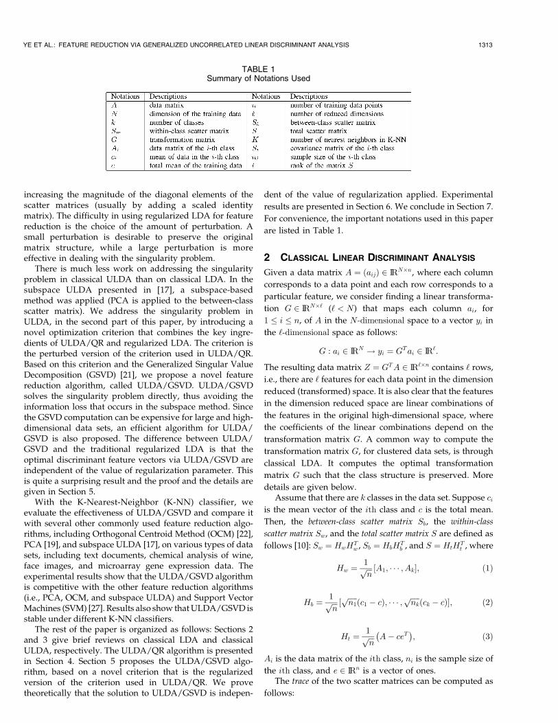
An efficient algorithm for computing f~xigqi¼1 throughQR-decomposition is presented below as Algorithm 1.

Algorithm 1: The ULDA/QR Algorithm

Input: Data matrix A.

Output: Discriminant vectors ~xis of ULDA.

1. Construct matrices Hw and Hb as in (1) and (2).

2. Compute the QR-decomposition of HTw as HT

w ¼ QR,

where Q 2 IRn�N and R 2 IRN�N .3. Form the matrix Y HT

b R�1.

4. Compute the SVD of Y as Y ¼ U�V T , where U 2 IRn�q,

� ¼ diagð�1; � � � ; �qÞ 2 IRq�q, V 2 IRN�q, �1 � � � � � �q,and q ¼ rankðHbÞ.

5. ½x1; � � � ; xq� R�1V .

6. �i �2i , for i ¼ 1; � � � ; q.

7. ~xi 1ffiffiffiffiffiffiffiffi1þ�ip xi, for i ¼ 1; � � � ; q.

5 THE ULDA/GSVD ALGORITHM

In the previous section, a variant of the classical LDAcriterion was presented in (7). It was shown that thesolution to the optimization problem in (7) forms optimaldiscriminant vectors for classical ULDA. Thus, it providesan efficient way for computing the optimal discriminantvectors for ULDA. However, the algorithm assumes thenonsingularity of Sw, which limits its applicability to low-dimensional data. In [17], a subspace-based method ispresented to overcome the singularity problem, where theULDA algorithm is preceded by PCA. However, the PCAstage may lose some useful information. In this section, wepropose a new feature reduction algorithm, called ULDA/GSVD. The new criterion underlying ULDA/GSVD ismotivated by the criterion in (7) and the regularized LDA.The new optimization problem for ULDA/GSVD is definedas follows:

G� ¼ arg maxGTSG¼I‘

F�ðGÞ; ð11Þ

where F�ðGÞ ¼ trace ðGTSwGþ �I‘Þ�1GTSbG� �

. Note that

matrix GTSwGþ �I‘ is guaranteed to be nonsingular for

� > 0.Recall that a limitation of regularized LDA is that the

optimal value of the perturbation� is difficult to determine. Akey difference between ULDA/GSVD and regularized LDAis that the optimal solution to ULDA/GSVD is independentof the regularization parameter, i.e., G�1

¼ G�2, for any

�1; �2 > 0. The main result of this section is summarized inthe following theorem:

Theorem 3. Let G�, for any � > 0, be the optimal solution to theoptimization problem in (11). Then, the following equalityholds:

G�1¼ G�2

; for any �1; �2 > 0: ð12Þ

To prove Theorem 3, we first show how to compute G�,for any � > 0. Recall that when the within-class scattermatrix is nonsingular, the optimal transformation can becomputed by finding the matrix X, which simultaneouslydiagonalizes the scatter matrices. For this, the GeneralizedSingular Value Decomposition (GSVD) can be applied, even

when both matrices are singular. A simple algorithm to

compute GSVD can be found in [15], where the algorithm is

based on [21].The computation of G�, for any � > 0, is based on the

following two lemmas:

Lemma 1. Let Sw, Sb, and S be defined as in Section 2, and let

t ¼ rankðSÞ. Then, there exists a nonsingular matrix

X 2 IRN�N , such that

XTSbX ¼ D1 ¼ diagð�21; � � � ; �2

t ; 0; � � � ; 0Þ; ð13Þ

XTSwX ¼ D2 ¼ diagð�21 ; � � � ; �2

t ; 0; � � � ; 0Þ; ð14Þ

where

1 � �1 � � � � � �q > 0 ¼ �qþ1 ¼ � � � ¼ �t;0 � �1 � � � � � �t � 1;

D1 þD2 ¼It 0

0 0

;

and q ¼ rankðSbÞ.Proof. Let

K ¼ HTb

HTw

� �;

which is an ðnþ kÞ �N matrix. By the Generalized

Singular Value Decomposition [21], there exist orthogo-

nal matrices U 2 IRk�k, V 2 IRn�n, and a nonsingular

matrix X 2 IRN�N , such that

U 00 V

� �TKX ¼ �1 0

�2 0

� �; ð15Þ

where

�T1 �1 ¼ diagð�2

1; � � � ; �2t Þ; �T

2 �2 ¼ diagð�21 ; � � � ; �2

t Þ;1 � �1 � � � � � �q > 0 ¼ �qþ1 ¼ � � � ¼ �t;0 � �1 � � � � � �t � 1;

�2i þ �2

i ¼ 1, for i ¼ 1; � � � ; t, and q ¼ rankðHbÞ ¼ rankðSbÞ.Hence, HT

b X ¼ U �1 0½ �, and HTwX ¼ V �2 0½ �. It

follows that

XTSbX ¼ XTHbHTb X ¼

�T1 �1 00 0

� �¼ D1;

XTSwX ¼ XTHwHTwX ¼

�T2 �2 00 0

� �¼ D2;

where D1 þD2 ¼It 00 0

. tu

Lemma 2. Define a trace optimization problem as follows:

G ¼ arg maxGTG¼I‘

trace GTWG� ��1

GTBG� �

; ð16Þ

where W ¼ diagðw1; � � � ; wuÞ 2 IRu�u is a diagonal matrixwith 0 < w1 � � � � � wu, and B ¼ diagðb1; � � � ; buÞ 2 IRu�u

is also diagonal with b1 � � � � � bq > 0 ¼ bqþ1 ¼ � � � ¼ bu.Then, G? ¼ Iq; 0

� �Tsolves the optimization problem in (16)

with ‘ ¼ q.


Proof. It is clear that the constraint in the optimization in(16) is satisfied for G? with ‘ ¼ q. Next, we show that G?

solves the following optimization problem:

G ¼ arg maxG

trace GTWG� ��1

GTBG� �

: ð17Þ

It is well-known that the solution can be obtained bysolving the eigenvalue problem on W�1B since W isnonsingular. Note thatW�1B is diagonal and only the firstq diagonal entries are nonzero. Hence, ei, for i ¼ 1; � � � ; q, isthe eigenvector of W�1B corresponding to the ith largesteigenvalue, where ei ¼ 0; � � � ; 1; 0 � � � ; 0ð ÞT and the oneappears at the ith entry. Therefore, G? ¼ Iq; 0

� �Tsolves

the optimization in (17). tuWith Lemma 1 and Lemma 2, we can compute G�, for

any � > 0, as follows:

Theorem 4. Let the matrix X be defined as in Lemma 1, and letq ¼ rankðSbÞ. Then,

G� ¼ XIq0

solves the optimization problem in (11) with ‘ ¼ q.Proof. By Lemma 1, XTSbX ¼ D1, XTSwX ¼ D2, where the

two diagonal matrices D1 and D2 satisfy

D1 þD2 ¼It 00 0

:

It is easy to check that

ðG�ÞTSG� ¼ Iq; 0

� �XT ðSb þ SwÞX

Iq

0

¼ Iq; 0� �

ðD1 þD2ÞIq

0

¼ Iq;

i.e., the constraint in the optimization problem in (11) issatisfied. Next, we show that G� minimizes F�ðGÞ. Since

GTSbG ¼ GT ðX�1ÞT ðXTSbXÞX�1G ¼ ~GD1~GT ;

GTSwG ¼ GT ðX�1ÞT ðXTSwXÞX�1G ¼ ~GD2~GT ;

where ~G ¼ ðX�1GÞT , F�ðGÞ can then be rewritten as

F�ðGÞ ¼ trace ~GD2~GT þ �I‘

� ��1 ~GD1~GT

� �: ð18Þ

Let ~G ¼ GT1 ; GT

2

� �be a partition of ~G, such that

GT1 2 IR‘�t and GT

2 2 IR‘�ðN�tÞ. By the constraint that

GTSG ¼ I‘, we have

I‘ ¼ GTSG ¼ GT ðSw þ SbÞG ¼ GTSbGþGTSwG

¼ ~GD1~GT þ ~GD2

~GT ¼ ~GðD1 þD2Þ ~GT ¼ GT1G1:

Hence, F�ðGÞ in (18) can be rewritten as

F�ðGÞ ¼ trace GT1 Dt

2 þ �I‘� �

G1

� ��1GT

1Dt1G1

� �;

where Dt1 and Dt

2 are the tth leading submatrices of D1

and D2, respectively. It is clear that F�ðGÞ is independentof G2. Hence, we can simplify set G2 ¼ 0. Denote� ¼ Dt

2 þ �It� �

, which is a nonsingular and diagonalmatrix. It follows that

F�ðGÞ ¼ trace GT1 �G1

� ��1GT

1Dt1G1

� �:

The result then follows from Lemma 2, with W ¼ � andB ¼ Dt

1. tuTheorem 4 implies that the optimal solution G?

� to theoptimization problem in (11) only depends on X, which isdetermined by Hw and Hb, hence it is independent of �.That is, G�1

¼ G�2, for any �1; �2 > 0. This completes the

proof of the main result of this section, which is summar-ized in Theorem 3.

The computation of the optimal transformation G issummarized in Algorithm 2.

Algorithm 2: The ULDA/GSVD Algorithm

Input: Data matrix A

Output: Optimal transformation matrix G

1. Form Hb and Hw as in (2) and (1).2. Compute GSVD on the matrix pair ðHT

b ;HTwÞ to obtain the

matrix X, as in Lemma 1.

3. q rankðHbÞ.4. G ½X1; � � � ; Xq�.

5.1 Efficient Computation of Diagonalizing Matrix X

In Lemma 1, a nonsingular matrix X is computed byapplying GSVD, which may be expensive, especially forlarge matrices. A key property of X which leads to theoptimal solutionG is that it diagonalizes the scatter matricessimultaneously. In this section, we present an efficientalgorithm for computing the diagonalizing matrixXwithoutthe GSVD computation.

Let Ht ¼ U�V T be the SVD of Ht, where Ht is defined in(3), U 2 IRN�N and V 2 IRn�n are orthogonal, and � 2 IRN�n

is diagonal. Then,

S ¼ HtHTt ¼ U�V TV�TUT ¼ U��TUT :

That is, the eigen-decomposition of S can be obtained bycomputing the SVD of Ht. Let U ¼ ðU1; U2Þ be the partitionof U , such that U1 2 IRN�t and U2 2 IRN�ðN�tÞ, wheret ¼ rankðSÞ. Let ��T ¼ diag �2

t ; 0� �

, where �t 2 IRt�t isdiagonal and nonsingular. Since S ¼ Sb þ Sw, the nullspace, U2, of St also lies in the null space of Sb and Sw,that is, UT

2 SbU2 ¼ 0 and UT2 SwU2 ¼ 0. Hence,

�2t ¼ UT

1 SbU1 þ UT1 SwU1 ð19Þ

and

It ¼ ��1t UT

1 SbU1��1t þ ��1

t UT1 SwU1��1

t : ð20Þ

Recall from (2) that Sb ¼ HbHTb . Denote B ¼ ��1

t UT1 Hb and

let B ¼ P ~�QT be the SVD of B, where P and Q areorthogonal and ~� is diagonal. Then,

��1t UT

1 SbU1��1t ¼ P ~�~�TPT ¼ P�bP

T ;

where �b ¼ ~�~�T ¼ diagð�1; � � � ; �tÞ,

�1 � � � � � �q > 0 ¼ �qþ1 ¼ � � � ¼ �t;

and q ¼ rankðSbÞ. It can be verified that the matrix X belowdiagonalizes the three scatter matrices simultaneously:

X ¼ U ��1t P 00 I

: ð21Þ


The pseudocode for the computation of X is given in

Algorithm 3.

Algorithm 3: Efficient computation of diagonalizing

matrix X

Input: data matrix A

Output: matrix X

1. Form matrices Hb and Ht as in (2) and (3).

2. Compute SVD of Ht as Ht ¼ U1�tVT

1 .

4. B �tUT1 Hb.

5. Compute SVD of B as B ¼ P ~�QT ; q rankðBÞ.

6. X U��1t P 00 I

.

5.2 Relationship between ULDA/GSVD andULDA/QR

In this section, we show that ULDA/GSVD is equivalent to

ULDA/QR when the within-class scatter matrix Sw is

nonsingular. Therefore, ULDA/QR can be considered as a

special case of ULDA/GSVD when Sw is nonsingular. Note

that ULDA/GSVD is more general in the sense that it is

applicable regardless of the singularity of Sw.Recall that ULDA/QR involves the matrix X, which

satisfies

XTSwX ¼ IN;XTSbX ¼ � ¼ diagð�1; � � � ; �NÞ;

where �1 � � � � � �N .The final transformation matrix G ¼ ~x1; � � � ; ~xq

� �, where

~xi ¼ 1ffiffiffiffiffiffiffiffi1þ�ip xi, xi is the ith column of the matrix X. It follows

that

ðGÞTSG ¼ Iq; ð22Þ

ðGÞTSbG ¼ diag�1

1þ �1; � � � ; �q

1þ �q

: ð23Þ

Since fðxÞ ¼ x=ð1þ xÞ is an increasing function, we have

�1

1þ �1� � � � � �q

1þ �q:

Thus, the transformation matrix G from ULDA/QR

satisfies the conditions in Lemma 1 for ULDA/GSVD. That

is, ULDA/GSVD is equivalent to ULDA/QR, when the

within-class scatter matrix Sw is nonsingular. Note that

ULDA/QR is not applicable when Sw is singular. ULDA/

GSVD can thus be considered as an extension of ULDA/QR

for a singular within-class scatter matrix. In the following

experimental studies, we focus on the ULDA/GSVD

algorithm.We close this section by showing the classification

property of ULDA/GSVD and ULDA/QR:

Theorem 5. Let G be the optimal transformation matrix for

ULDA/GSVD. Then, for any test point h, the following

equality holds:

arg minjðh� cjÞTSþðh� cjÞn o

¼ arg minjjjGT ðh� cjÞjj2n o

:

Proof. Let Xi be the ith column of X. Note that G consists ofthe first q columns of X, and q ¼ rankðSbÞ. From (13) and(14), we have

Sþ ¼ XðD1 þD2ÞXT ¼ GGT þXti¼qþ1

XiXTi :

From (13), XTi SbXi ¼ 0, for i ¼ q þ 1; � � � ; t. Hence,

ðcjÞTXi ¼ cXi, for all j ¼ 1; � � � ; k. It follows that

ðh� cjÞTSþðh� cjÞ ¼ jjGT ðh� cjÞjj2þXti¼qþ1

ðh� cÞTXiXTi ðh� cÞ:

ð24Þ

The main result follows, since the second term on theright-hand side of (24) is independent of j. tuWhen S is nonsingular, the classification in ULDA/QR

uses the Mahalanobis distance measure as follows:

Corollary 1. Assume S is nonsingular. Let G be the optimaltransformation matrix for ULDA/QR. Then, for any test pointh, the following equality holds:

arg minjðh� cjÞTS�1ðh� cjÞn o

¼ arg minjjjGT ðh� cjÞjj2n o

:

Corollary 1 shows that the classification in ULDA/QR isbased on the Mahalanobis distance measure, while Theo-rem 5 shows that the classification in ULDA/GSVD is basedon the modified Mahalanobis distance measure.

6 EXPERIMENTS

We evaluate the effectiveness of the ULDA/GSVD algo-rithm in this section. Section 6.1 describes our test data sets.Section 6.2 examines the effect of the number of reduceddimensions on the classification performance of ULDA/GSVD. In Section 6.3, we compare ULDA/GSVD with PCA,OCM, and subspace ULDA, as well as SVM, in terms ofclassification accuracy. The K-Nearest-Neighbor (K-NN)algorithm with different values of K is used as the classifier.

6.1 Data Sets

We used two data sets: Spambase and Wine from the UCIMachine Learning Repository.3 We used a subset of theoriginal Spambase data set, which consists of spam andnonspam emails. Most of the features indicate whether aparticular word or character occurred frequently in thee-mail. The Wine data set is the result of a chemical analysisof wines grown in the same region in Italy but derived fromthree different cultivars. The features correspond to thequantities of 13 different constituents found in each of thethree types of wines. For these two data sets, the datadimension (N) is much smaller than the sample size (n). Wealso used six other data sets: GCM, ALL, tr41, re1, PIX, andORL, where the data dimension is much larger than thesample size. In this case, ULDA/QR is not applicable, sinceall scatter matrices are singular, while ULDA/GSVD is stillapplicable. GCM [23], [30] and ALL [31] are microarraygene expression data sets; tr41 is a document data set


3. http://www.ics.uci.edu/mlearn/MLRepository.html.

derived from the TREC-5, TREC-6, and TREC-7 collections;4

re1 is another document data set derived from Reuters-21578text categorization test collection Distribution 1.0;5 andORL6 and PIX 7 are two face image data sets.

Table 2 summarizes the statistics of our test data sets.

6.2 Effect of the Number of Reduced Dimensions onULDA/GSVD

In this experiment, we study the effect of the number ofreduced dimensions on the classification performance ofULDA/GSVD. The number of reduced dimensions rangesfrom 1 to 20. The classification results on the GCM and ALLdata sets are shown in Fig. 1, where the horizontal axis isthe number of reduced dimensions and the vertical axis isthe classification accuracy. We can observe that theaccuracy tends to increase when the number of reduceddimensions increases, until q ¼ rankðHbÞ (13 for GCM and 5for ALL) is reached. Similar trends have been observedfrom other data sets, and the results are not presented. Inthe following experiment, we set the reduced dimension ofULDA/GSVD to be the rank of Hb.

6.3 Comparison of Classification Accuracy

In this experiment, we applied ULDA/GSVD to the eightdata sets from Table 2 and compared with OCM, PCA, andsubspace ULDA in terms of classification accuracy. Theresults are summarized in Table 3. The number of principalcomponents used in PCA and Subspace ULDA is deter-mined through cross-validation, and may be different fordifferent data sets.

For data sets, including Spambase, Wine, GCM, andALL, the training and test sets given in the original data setsare used for computing the accuracy. For the other four datasets, including tr41, re1, PIX, and ORL, where the trainingand test sets are not given, we performed our study byrepeated random splitting into training and test sets exactlyas in [7]. The data was partitioned randomly into a trainingset consisting of two-thirds of the whole set and a test setconsisting of one-third of the whole set. To reduce thevariability, the splitting was repeated 50 times and theresulting accuracies were averaged. The standard deviationfor each data set was also reported.

The main observations from Table 3 include: 1) ULDA/GSVD is competitive with the other three algorithms for alldata sets in terms of classification. Subspace ULDA per-forms well for most data sets. However, subspace ULDAapplies cross-validation for determining the optimal set ofprincipal components in the PCA step, which can beexpensive, especially for large data sets. Besides, thevariance of the results for the other three methods isgenerally larger than that of ULDA/GSVD. This impliesthat ULDA/GSVD provides a more consistent result.2) ULDA/GSVD is extremely stable under different K-NNclassifiers for all data sets, whereas the performance ofOCM and PCA degrades for many cases, as the number, K,of nearest neighbors increases. Subspace ULDA is alsostable under different K-NN classifiers for most data sets.3) PCA does not perform well in many cases. This is likelyrelated to the fact that PCA is unsupervised and does notuse the class label information, while the other threealgorithms fully utilize the class label information. OCMperforms well for the two document data sets and the twoface image data sets, while it performs poorly for the otherdata sets. Both PCA and OCM perform poorly in Spambaseand Wine, in comparison with ULDA/GSVD and subspaceULDA.

We have also done some preliminary studies in comparingULDA/GSVD with linear SVM. 1NN is used to compute theaccuracy for ULDA/GSVD. The main result is summarized inFig. 2, where the x-axis denotes the eight data sets, and they-axis denotes the classification accuracy. For tr41, re1, PIX,and ORL, the mean accuracy for 50 different runs arereported. Overall, ULDA/GSVD and linear SVM are compar-able in terms of classification.

7 CONCLUSION

Uncorrelated features with minimum redundancy arehighly desirable in feature reduction. In this paper, wepresent a theoretical and empirical study on uncorrelatedLinear Discriminant Analysis (ULDA). We first present thetheoretical result on the equivalence relationship betweenclassical ULDA and classical LDA, which leads to a fastimplementation of ULDA, ULDA/QR. Then, we proposeULDA/GSVD, based on a novel optimization criterion, thatcan successfully overcome the singularity problem inclassical ULDA. The criterion used in ULDA/GSVD is theperturbed version of the one from ULDA/QR, while thesolution to ULDA/GSVD is shown to be independent of theamount of perturbation applied, thus avoiding the limita-tion in regularized LDA. Experimental results on varioustypes of data show the superiority of ULDA/GSVD overother competing algorithms including PCA, OCM, andsubspace ULDA.

Experimental results show that ULDA/GSVD is extre-

mely stable under different K-NN classifiers for all data

sets. We plan to carry out detailed theoretical analysis on

this in the future. The current work focuses on linear

discriminant analysis, which applies a linear decision

boundary. Discriminant analysis can also be studied in a

nonlinear fashion—so-called kernel discriminant analysis—

by using the kernel trick [24]. This is desirable if the data


4. http://trec.nist.gov.5. http://www.research.att.com/~lewis.6. http://www.uk.research.att.com/facedatabase.html.7. http://peipa.essex.ac.uk/ipa/pix/faces/manchester/test-hard/.

TABLE 2Statistics for the Test Data Sets

(“—” means that the natural splitting of the data set into training and testset is not available. For Spambase, Wine, GCM, and ALL, the originaltraining and test sets are given, while for tr41, re1, PIX, and ORL, theoriginal splitting is not provided.)

has weak linear separability. We plan to extend the current

work to deal with the nonlinearity in the future.

ACKNOWLEDGMENTS

The authors would like to thank the four reviewers and theassociate editor for their comments, which helped improve

the paper significantly. The research of J. Ye and R.Janardan was sponsored, in part, by the Army HighPerformance Computing Research Center under the aus-pices of the Department of the Army, Army ResearchLaboratory cooperative agreement number DAAD19-01-2-0014, the content of which does not necessarily reflect theposition or the policy of the government, and no official


TABLE 3Comparison of Classification Accuracy on Four Different Methods

Fig. 1. Effect of the number of reduced dimensions on the classification performance of ULDA/GSVD for (a) the GCM and (b) ALL data sets. The

optimal numbers of reduced dimensions for GCM and ALL are 13 and 5, respectively.

endorsement should be inferred. Fellowships from Guidant

Corporation and from the Department of Computer Science

and Engineering, at the University of Minnesota, Twin

Cities are gratefully acknowledged. The work of H. Park

has been performed while serving as a program director at

the US National Science Foundation (NSF) and was partly

supported by IR/D from the NSF. Her work was also

supported in part by the US National Science Foundation

Grants CCR-0204109 and ACI-0305543. Any opinions,

findings, and conclusions or recommendations expressed

in this material are those of the authors and do not

necessarily reflect the views of the US National Science

Foundation.

REFERENCES

[1] P. Belhumeour, J. Hespanha, and D. Kriegman, “Eigenfaces vs.Fisherfaces: Recognition Using Class Specific Linear Projection,”IEEE Trans. Pattern Analysis and Machine Intelligence, vol. 19, no. 7,pp. 711-720, 1997.

[2] M. Berry, S. Dumais, and G. O’Brie, “Using Linear Algebra forIntelligent Information Retrieval,” SIAM Rev., vol. 37, pp. 573-595,1995.

[3] L. Chen, H. Liao, M. Ko, J. Lin, and G. Yu, “A New LDA-BasedFace Recognition System Which Can Solve the Small Sample SizeProblem,” Pattern Recognition, vol. 33, pp. 1713-1726, 2000.

[4] S. Deerwester, S. Dumais, G. Furnas, T. Landauer, and R.Harshman, “Indexing by Latent Semantic Analysis,” J. Soc. forInformation Science, vol. 41, pp. 391-407, 1990.

[5] L. Duchene and S. Leclerq, “An Optimal Transformation forDiscriminant and Principal Component Analysis,” IEEE Trans.Pattern Analysis and Machine Intelligence, vol. 10, no. 6, pp. 978-983,1988.

[6] R. Duda, P. Hart, and D. Stork, Pattern Classification. Wiley, 2000.[7] S. Dudoit, J. Fridlyand, and T.P. Speed, “Comparison of

Discrimination Methods for the Classification of Tumors UsingGene Expression Data,” J. Am. Statistical Assoc., vol. 97, no. 457,pp. 77-87, 2002.

[8] D. Foley and J. Sammon, “An Optimal Set of DiscriminantVectors,” IEEE Trans. Computers, vol. 24, no. 3, pp. 281-289, 1975.

[9] J. Friedman, “Regularized Discriminant Analysis,” J. Am. Statis-tical Assoc., vol. 84, no. 405, pp. 165-175, 1989.

[10] K. Fukunaga, Introduction to Statistical Pattern Classification.Academic Press, 1990.

[11] G.H. Golub and C.F. Van Loan, Matrix Computations, third ed. TheJohns Hopkins Univ. Press, 1996.

[12] T. Hastie, A. Buja, and R. Tibshirani, “Penalized DiscriminantAnalysis,” Annals of Statistics, vol. 23, pp. 73-102, 1995.

[13] T. Hastie and R. Tibshirani, “Discriminant Analysis by GaussianMixtures,” J. Royal Statistical Soc. series B, vol. 58, pp. 158-176, 1996.

[14] T. Hastie, R. Tibshirani, and J. Friedman, The Elements of StatisticalLearning: Data Mining, Inference, and Prediction. Springer, 2001.

[15] P. Howland, M. Jeon, and H. Park, “Structure PreservingDimension Reduction for Clustered Text Data Based on theGeneralized Singular Value Decomposition,” SIAM J. MatrixAnalysis and Applications, vol. 25, no. 1, pp. 165-179, 2003.

[16] P. Howland and H. Park, “Generalizing Discriminant AnalysisUsing the Generalized Singular Value Decomposition,” IEEETrans. Pattern Analysis and Machine Intelligence, vol. 26, no. 8,pp. 995-1006, Aug. 2004.

[17] Z. Jin, J.Y. Yang, Z.-S. Hu, and Z. Lou, “Face Recognition Based onthe Uncorrelated Discriminant Transformation,” Pattern Recogni-tion, vol. 34, pp. 1405-1416, 2001.

[18] Z. Jin, J.-Y. Yang, Z.-M. Tang, and Z.-S. Hu, “A Theorem on theUncorrelated Optimal Discriminant Vectors,” Pattern Recognition,vol. 34, no. 10, pp. 2041-2047, 2001.

[19] I.T. Jolliffe, Principal Component Analysis. Springer-Verlag, 1986.[20] W. Krzanowski, P. Jonathan, W. McCarthy, and M. Thomas,

“Discriminant Analysis with Singular Covariance Matrices:Methods and Applications to Spectroscopic Data,” AppliedStatistics, vol. 44, pp. 101-115, 1995.

[21] C. Paige and M. Saunders, “Towards a Generalized SingularValue Decomposition,” SIAM J. Numerical Analysis, vol. 18,pp. 398-405, 1981.

[22] H. Park, M. Jeon, and J. Rosen, “Lower Dimensional Representa-tion of Text Data Based on Centroids and Least Squares,” BITNumerical Math., vol. 43, no. 2, pp. 1-22, 2003.

[23] S. Ramaswamy et al., “Multiclass Cancer Diagnosis Using TumorGene Expression Signatures,” Proc. Nat’l Academy of Science,vol. 98, no. 26, pp. 15149-15154, 2001.

[24] B. Schokopf and A. Smola, Learning with Kernels: Support VectorMachines, Regularization, Optimization and Beyond. MIT Press, 2002.

[25] D.L. Swets and J. Weng, “Using Discriminant Eigenfeatures forImage Retrieval,” IEEE Trans. Pattern Analysis and MachineIntelligence, vol. 18, no. 8, pp. 831-836, Aug. 1996.

[26] M. Turk and A. Pentland, “Face Recognition Using Eigenfaces,”Proc. Computer Vision and Pattern Recognition Conf., pp. 586-591,1991.

[27] V. Vapnik, Statistical Learning Theory. Wiley, 1998.[28] J. Ye, “Characterization of a Family of Algorithms for Generalized

Discriminant Analysis on Undersampled Problems,” J. MachineLearning Research, vol. 6, pp. 483-502, 2005.

[29] J. Ye, R. Janardan, C. Park, and H. Park, “An OptimizationCriterion for Generalized Discriminant Analysis on Under-sampled Problems,” IEEE Trans. Pattern Analysis and MachineIntelligence, vol. 26, no. 8, pp. 982-994, Aug. 2004.

[30] C.H. Yeang et al., “Molecular Classification of Multiple TumorTypes,” Bioinformatics, vol. 17, no. 1, pp. 1-7, 2001.

[31] E.J. Yeoh et al., “Classification, Subtype Discovery, and Predictionof Outcome in Pediatric Lymphoblastic Leukemia by GeneExpression Profiling,” Cancer Cell, vol. 1, no. 2, pp. 133-143, 2002.


Fig. 2. Comparison of classification accuracy between ULDA/GSVD and SVM. For tr41, re1, PIX, and ORL, the mean accuracy for 50 different runs

are reported.

Jieping Ye received the PhD degree in compu-ter science from the University of Minnesota-Twin Cities in 2005. He is an assistant professorin the Department of Computer Science andEngineering at Arizona State University. He wasawarded the Guidant Fellowship in 2004-2005.In 2004, his paper on generalized low rankapproximations of matrices won the outstandingstudent paper award at the 21st InternationalConference on Machine Learning. His research

interests include data mining, machine learning, and bioinformatics. Heis a member of the IEEE and the ACM.

Ravi Janardan received the PhD degree incomputer science from Purdue University in1987. He is a professor in the Department ofComputer Science and Engineering at theUniversity of Minnesota-Twin Cities. His re-search interests are in the design and analysisof geometric algorithms and data structures andtheir application to problems in a variety ofareas, including computer-aided design andmanufacturing, computational biology and bioin-

formatics, and query retrieval in geometric databases. He has publishedextensively in these areas. He is a senior member of the IEEE and theIEEE Computer Society. He serves on the editorial board of the Journalon Discrete Algorithms and on the editorial advisory board of CurrentBioinformatics.

Qi Li received the BS degree from the Depart-ment of Mathematics, Zhongshan University,China, in 1993, and the MS degree from theDepartment of Computer Science, University ofRochester, in 2002. He is currently a PhDcandidate in the Department of Computer andInformation Sciences, University of Delaware.His current research interests include patternrecognition, data mining, and machine learning.He is a student member of the IEEE.

Haesun Park received the BS degree inmathematics from Seoul National University,Seoul, Korea, in 1981 summa cum laude andwith the university president’s medal for the topgraduate, and the MS and PhD degrees incomputer science from Cornell University, Itha-ca, New York, in 1985 and 1987, respectively.She was on the faculty of the Department ofComputer Science and Engineering, Universityof Minnesota, Twin Cities, from 1987 to 2005.

Since July 2005, she has been a professor in the College of Computing,Georgia Institute of Technology, Atlanta. Dr. Park has published morethan 100 refereed journal and conference proceedings papers. Hercurrent research interests include numerical algorithms, pattern recogni-tion, data mining, information retrieval, and bioinformatics. She servedon numerous conference committees and editorial boards of journals.Currently, she is on the editorial board of BIT Numerical Mathematics,the SIAM Journal on Matrix Analysis and Applications, and theInternational Journal on Bioinformatics Research and Applications.From 2003 to 2005, Dr. Park served as a program director for theComputing and Communication Foundations Division at the US NationalScience Foundation, Arlington, Virginia.

. For more information on this or any other computing topic,please visit our Digital Library at www.computer.org/publications/dlib.


Documents

Feature Reduction via Generalized Uncorrelated Linear ...jye02/Publications/Papers/gulda_tkde06.pdf · Feature Reduction via Generalized Uncorrelated Linear Discriminant Analysis