Embed Size (px)
Citation preview

NIST Technical Note 1774
FDD CX: A Fault Detection and Diagnostic Commissioning Tool for
Residential Air Conditioners and Heat Pumps
Jaehyeok Heo W. Vance Payne
Piotr A. Domanski
http://dx.doi.org/10.6028/NIST.TN.1774
NIST Technical Note 1774
FDD CX: A Fault Detection and Diagnostic Commissioning Tool for
Residential Air Conditions and Heat Pumps
Jaehyeok Heo
W. Vance Payne Piotr A. Domanski
Energy and Environment Division Engineering Laboratory
http://dx.doi.org/10.6028/NIST.TN.1774
November 2012
U.S. Department of Commerce Rebecca Blank, Acting Secretary
National Institute of Standards and Technology
Patrick D. Gallagher, Under Secretary of Commerce for Standards and Technology and Director

Certain commercial entities, equipment, or materials may be identified in this
document in order to describe an experimental procedure or concept adequately. Such identification is not intended to imply recommendation or endorsement by the National Institute of Standards and Technology, nor is it intended to imply that the entities, materials, or equipment are necessarily the best available for the purpose.
Use of Non-SI Units in a NIST Publication The policy of the National Institute of Standards and Technology is to use the International System of Units (metric
units) in all of its publications. However, in North America in the heating, ventilation and air-conditioning industry, certain non-SI units are so widely used instead of SI units that it is more practical and less confusing to include some
measurement values in customary units only.
Software Disclaimer This software was developed at the National Institute of Standards and Technology by employees of the Federal Government in the course of their official duties. Pursuant to title 17 Section 105 of the United States Code this
software is not subject to copyright protection and is in the public domain. These programs are experimental systems. NIST assumes no responsibility whatsoever for their use by other parties, and makes no guarantees,
expressed or implied, about its quality, reliability, or any other characteristic. We would appreciate acknowledgement if the software is used. This software can be redistributed and/or modified freely provided that
any derivative works bear some notice that they are derived from it, and any modified versions bear some notice that they have been modified.
National Institute of Standards and Technology Technical Note 1774 Natl. Inst. Stand. Technol. Tech. Note 1774, 33 pages (November 2012)
http://dx.doi.org/10.6028/NIST.TN.1774 CODEN: NTNOEF

Contents 1. Introduction ................................................................................................................................ 1 2. Installation .................................................................................................................................. 2 3. Using FDD CX .............................................................................................................................. 3
3.1. System Information .............................................................................................................. 3 3.2. Fault Detection and Diagnostics ........................................................................................... 8 3.3. FDD Results Graphs ............................................................................................................ 10
3.4. About FDD CX ..................................................................................................................... 12
3.5. Guidance on Adjusting Correction Factors ........................................................................ 13
3.6. Guidance on Adjusting Thresholds .................................................................................... 14
4. Application Example ................................................................................................................. 16
4.1. Enter the System Information ........................................................................................... 16
4.2. Run Fault Detection and Diagnostics ................................................................................. 17
4.3. Examine FDD Result Graphs .............................................................................................. 20 5. The Fault Detection and Diagnosis Method ............................................................................. 22 References .................................................................................................................................... 25 Acknowledgements ....................................................................................................................... 26

1
1. Introduction In earlier work the National Institute of Standards and Technology (NIST) made detailed measurements on the cooling (Payne, Domanski, & Hermes, 2006) and heating [ (Payne, Domanski, & Yoon, 2009), (Yoon, Payne, & Domanski, 2011)] performance of a residential, split-system, air source, heat pump with faults imposed. The previous research on FDD techniques was examined [e.g., (Rossi & Braun, 1997), (Braun, 1999), (Chen & Braun, 2001)] and used to refine the rule-based chart technique of fault detection and diagnostics of common faults which can occur during operation of an air conditioner (AC) and heat pump (HP) [ (Kim M. , Yoon, Payne, & Domanski, 2008).
While an AC or HP may exhibit a range of faults during its operational life, the list of most common faults resulting from improper installation is smaller, with the most prevalent being refrigerant undercharge, refrigerant overcharge, and improper indoor air flow. The prevalence of these three commissioning faults provided a motivation for developing a standalone software tool that incorporated these “commissioning mode” features. The generic nature of the FDD method allows this technique to be applied to split systems equipped with thermostatic expansion valves (TXVs), which represent a majority of residential and light commercial systems installed today.
This FDD based commissioning tool software is meant to be applied to residential, unitary, air-source, single-speed, vapor compression air-conditioning (AC) or heat pump (HP) systems with nominal cooling capacities less than 19 kW (≈65 000 Btu h-1 or 5.4 tons). Air and refrigerant temperatures plus refrigerant saturation temperatures need to be measured throughout the system and input into the program to determine proper refrigerant charge and indoor air flow.

2
2. Installation
2.1. PC System Requirements
Personal computer (PC) with Microsoft® Windows® 7, XP with Service Pack 3, and Vista operating systems.
Free space for complete installation: 10.0 MB
The installation module requires .NET Framework 2.0 Service Pack 2 (or later version), which can be downloaded from the Microsoft website if not present on the user’s PC.
2.2. Installation Procedure
Click [Start], select [Run], type: D:\NIST FDD CX Ver. 1.0.msi, or use the appropriate letter associated with the drive and directory on which the installation module is located, and press [Enter].
Follow the on screen instructions.
If FDD CX is installed using the default locations, the executable file will be placed in C:\Program Files\NIST\FDD CX, and files with example compressor maps and example data will be placed in \NIST\FDD CX\data\compressor maps and \NIST\FDD CX\data\examples subdirectories, respectively.

3
3. Using FDD CX The user selects COOLING or HEATING in the FDD CX opening window of Figure 1, then the graphical user interface (GUI) displays the main screen with the System Information tab open. The user interacts with FDD CX through the GUI, which consists of three main parts: System Information, Fault Detection and Diagnostics, and FDD Result Graphs. The fourth tab, About FDD CX, provides general information about the software.
Figure 1. Opening screen for selecting cooling or heating mode
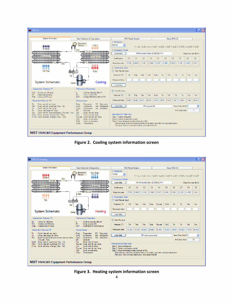
3.1. System Information
The System information tab is shown in Figure 2 and Figure 3 for the cooling and heating modes, respectively. The sequence of steps the user is required to take is listed at the bottom on the right hand side of the screen.
Step 1. Select refrigerant
Refrigerant type (R410A, R22,.etc.) is selected to allow calculation of refrigerant properties.
Step 2. Select compressor model
Compressor mass flow rate coefficients are selected by clicking the Load data button, which accesses a spreadsheet file that must be constructed as described in Section 4. A complete description of compressor map equations may be found in (AHRI, 2004). A common source of the compressor mass flow rate coefficients may be the online resources provided by the compressor manufacturer; using the compressor model number, the coefficients may be found.
4
Figure 2. Cooling system information screen
Figure 3. Heating system information screen

5
If the compressor mass flow rate coefficients cannot be found, use an example compressor data file found under \NIST\FDD CX\data\compressor maps\; the mass flow rate map is used to predict capacity and efficiency only and will not affect fault detection.
Figure 4. Compressor map mass flow rate coefficients data file format example
Step 3. Input data
Input of data (temperatures or temperature-based variables) measured on the AC or HP, may be performed manually, by entering data using the GUI, or by loading the data from a file stored on the PC. If the user wants to manually enter the temperature data, they select the Use Manual Input button, and then enter the temperatures one-by-one into the data table. If the user selects Use File Input, they select the Load Data button and use the File Explorer to select the spreadsheet file that contains the data.
The user must enter 11 cooling or 10 heating temperatures or temperature based variables. Table 1 and Table 2 list and describe the inputs and measurement locations for the cooling and heating modes, respectively.

6
Table 1. Cooling temperature input descriptions
Feature Name Description
Tid Indoor air dry-bulb temperature. Indoor air handler return (inlet) air dry-bulb temperature (°F)
Tidp Indoor air dewpoint temperature. Indoor air handler return (inlet) air dewpoint temperature (°F)
Tido Evaporator air exit temperature. Indoor air handler supply (exit) air dry-bulb temperature (°F)
Tod Outdoor air dry-bulb temperature. Outdoor unit inlet air dry-bulb temperature (°F)
Todo Condenser air exit temperature. Outdoor unit exit air dry-bulb temperature (°F)
Te Evaporator exit refrigerant saturation temperature. Refrigerant saturation temperature at the vapor line service valve pressure (°F)
Tsh Evaporator exit refrigerant superheat. Refrigerant temperature minus the saturation temperature at the vapor line service valve pressure (°F)
Td Compressor discharge refrigerant temperature (°F) [Measured at the discharge port of the compressor. ]
Tc Condenser inlet refrigerant saturation temperature. Refrigerant saturation temperature at the liquid line service port pressure (°F)
Tsc Condenser exit refrigerant subcooled temperature. Refrigerant saturation temperature minus liquid temperature at the liquid line service port (°F)
Tco Condenser exit refrigerant temperature. Refrigerant temperature at the liquid line service port (°F)

7
Table 2. Heating temperature input descriptions
Feature Name Description
Tid Indoor air dry-bulb temperature. Indoor air handler return (inlet) air dry-bulb temperature (°F)
Tido Evaporator air exit temperature. Indoor air handler supply (exit) air dry-bulb temperature (°F)
Tod Outdoor air dry-bulb temperature. Outdoor unit inlet air dry-bulb temperature (°F)
Todp Outdoor air dewpoint temperature. Outdoor unit air dewpoint temperature (°F)
Teo,sat Evaporator exit refrigerant saturation temperature. Refrigerant saturation temperature at the suction service port pressure (°F)
TshE Evaporator exit refrigerant superheat. Refrigerant temperature minus the saturation temperature at the suction service port pressure (°F)
Td Compressor discharge refrigerant temperature (°F) [Measured at the discharge port of the compressor.]
Tc Condenser inlet refrigerant saturation temperature. Refrigerant saturation temperature at the vapor line service port pressure (°F)
Tsc Liquid line subcooling at the outdoor service valve. Refrigerant saturation temperature minus liquid temperature at the liquid line service port (°F)
Tco Condenser exit refrigerant temperature. Refrigerant temperature at the liquid line service port (°F)
If the user selects the Manual Input option, the temperatures are entered in the table. Once all of the required temperatures are entered, the user clicks on Load Data to update the data values used in the calculations.
If the user selects the Use File Input option, the user must then click the Load Data button and navigate to the data file containing the temperature values. Figure 5 and Figure 6 show example spreadsheet data files for the cooling and heating modes, respectively.
Figure 5. Cooling example data file

8
Figure 6. Heating example data file
The first line of the data file may contain any kind of text information such as a description of the data file, the second line of information may be any kind of text such as the temperature labels, and the following lines can be one or more temperature data sets. The first two lines are not used by the program and are skipped during the input process. The “END” statement must be included in the first column and last row of the data file to indicate the end of the temperature data.
3.2. Fault Detection and Diagnostics
Once the required system information has been provided, the user can move to the Fault Detection and Diagnostics screen as shown in Figures 7 and 8 for the cooling and heating modes, respectively. The sequence of steps the user should take is listed at the bottom of the screen.
Step 1. Adjust correction factors (optional)
If the user is familiar with the system being tested, correction factors may be input into the table. The temperature corrections (positive or negative) allow the predicted, no-fault temperatures (features) to be corrected to more closely match system data. The correction factors (abbreviated as Corr. fac.) are used when the user has a large set of no-fault data at different outdoor and indoor temperatures with which to correct the predicted features. Section 3.5 provides additional guidance on using this option.
Step 2. Adjust thresholds (optional)
If the user has a large set of no-fault data, they may also adjust the Threshold values to maximize the No-Fault Probability. Here the user may select appropriate Threshold values for the temperature residuals used by the FDD logic to determine system performance. Under the Threshold label, the user clicks the drop-down menu and selects Default, Tested, or Manual values of threshold temperature differences: Default threshold values were selected to produce a wide tolerance for measurement uncertainty while maintaining fault detection sensitivity; Tested threshold values were determined from laboratory testing; Manual threshold values allow the user to input a value. The temperature residual is defined as the measured value minus the predicted value. The threshold defines the no-fault temperature difference value and is the amount of change in a temperature residual that is still considered neither

9
positive nor negative; meaning that the temperature residual can vary up to the threshold amount, above and below zero, before it is considered a non-zero value. Ideally, the residuals will all equal zero if the predicted and measured temperature variables are equal.
Figure 7. Cooling fault detection and diagnosis screen
10
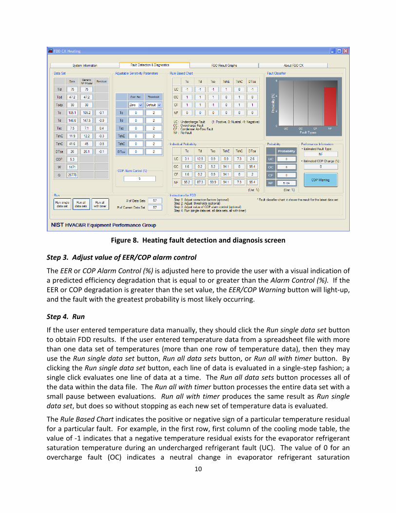
Figure 8. Heating fault detection and diagnosis screen
Step 3. Adjust value of EER/COP alarm control
The EER or COP Alarm Control (%) is adjusted here to provide the user with a visual indication of a predicted efficiency degradation that is equal to or greater than the Alarm Control (%). If the EER or COP degradation is greater than the set value, the EER/COP Warning button will light-up, and the fault with the greatest probability is most likely occurring.
Step 4. Run
If the user entered temperature data manually, they should click the Run single data set button to obtain FDD results. If the user entered temperature data from a spreadsheet file with more than one data set of temperatures (more than one row of temperature data), then they may use the Run single data set button, Run all data sets button, or Run all with timer button. By clicking the Run single data set button, each line of data is evaluated in a single-step fashion; a single click evaluates one line of data at a time. The Run all data sets button processes all of the data within the data file. The Run all with timer button processes the entire data set with a small pause between evaluations. Run all with timer produces the same result as Run single data set, but does so without stopping as each new set of temperature data is evaluated.
The Rule Based Chart indicates the positive or negative sign of a particular temperature residual for a particular fault. For example, in the first row, first column of the cooling mode table, the value of -1 indicates that a negative temperature residual exists for the evaporator refrigerant saturation temperature during an undercharged refrigerant fault (UC). The value of 0 for an overcharge fault (OC) indicates a neutral change in evaporator refrigerant saturation

11
temperature. A neutral change means that the temperature residual does not vary more than plus or minus the threshold value. A positive one (1) indicates a positive temperature difference for refrigerant superheat with an undercharge fault.
The cells within the Individual Probability table, shown in Figure 7 and Figure 8, correspond directly with the cells in the Rule Based Chart table. For example, Row 1, Column 1 of the Individual Probability table in Figure 7 is the probability, P between 0 and 1, that Te has a negative temperature residual based upon the threshold value used.
The Probability table indicates the total probability of an Undercharge fault (UC), overcharge fault (OC), indoor air flow fault (EF in cooling, CF in heating), or No-Fault (NF). The numeric values shown in this table are also plotted in the Fault Classifier chart.
The Fault Classifier chart shows different height bars with the tallest bar indicating the most likely fault condition including no-fault probability.
Performance Information shows the abbreviation of the most likely fault condition, the estimated change in system efficiency (EER/COP), and the EER/COP Warning light. The warning light will change color if the estimated change in system efficiency is greater than or equal to the Alarm Control (%) value.
3.3. FDD Result Graphs
Once the user has selected Run data on the Fault Detection and Diagnostics tab, they may examine the averaged fault detection and diagnostic statistics on the FDD Result Graphs screen shown in Figure 9 and Figure 10 for the cooling and heating modes, respectively. If the user were processing the data in single steps or using the Run all with timer from the Fault Detection and Diagnostics screen, the averaged parameters are updated for those temperature data sets processed thus far; the averaged parameters would not be indicative of the averages for the entire data set. If the user has selected Run all data sets, then the averages presented would be averages for the entire data set.

12
Figure 9. Cooling FDD results graphs screen for a no-fault condition
Figure 10. Heating FDD results graphs screen for a no-fault condition

13
The average probability of a fault is shown graphically on the far left of the screen. Four fault conditions, including the NF (No-Fault) condition, are shown as red bars. The condition with the highest probability of occurrence will have the tallest bar in this graph. The numeric values of the individual probability percentages are shown in the table below the graph. In the example shown in Figure 9, NF or No-Fault, has the highest probability.
The center graph in Figure 9 shows the average values of the temperature residuals. If the measured (input) values were identical to the predicted values (no-fault values), the residuals would be exactly zero. Since the data that was processed to generate Figure 9 was No-Fault data, the residuals are very small and are much less than the temperature threshold values entered on the Fault Detection and Diagnostics screen.
The graph on the right side of Figure 9 shows the predicted percentage degradation in system performance due to the most likely fault. Since this graph was generated with no-fault data, the residuals are close to zero indicating a no-fault system.
3.4. About FDD CX
The user may select the About FDD CX tab to read background information on the software as shown in Figure 11. Contact information for any software questions or comments is also provided on this screen.
Figure 11. Background information screen for FDD CX

14
3.5 Guidance on Adjusting Correction Factors
If the user has no-fault data (such as Cooling NF example.xlsx and Heating NF examples.xlsx files in the \NIST\FDD CX\data\examples subdirectory), they may run FDD CX and compare the measured and predicted features to determine appropriate correction factors. These correction factors should ideally include a range of outdoor and indoor temperature conditions, and at the least, should include several data sets. Correction factors are just additive offsets that may be used to help the generic no-fault model predictions more closely match no-fault measured data.
The FDD methodology depends on evaluating differences between the temperature values (features) measured during system operation and the values considered to be “correct” values for a fault-free system. These “correct” or “no-fault” values are calculated by FDD CX as a function of indoor and outdoor conditions based on measurements taken in environmental chambers on a fault-free residential heat pump. While the general trends of the calculated features are expected to be very similar for all vapor compression systems, absolute values of these features may differ due to differences in components used in different systems. For this reason, the Fault Detection and Diagnostics screen provides an option to input correction parameters for the FDD features to provide an offset, thus accounting for these differences.
Since refrigerant subcooling is the most influential feature for determining the proper refrigerant charge in the system, we have included Figures 12 and 13 to show the generic no-fault model’s predictions for Tsc as a function of outdoor temperature for the cooling and heating modes, respectively. . If the installer has knowledge of the proper system subcooling for a given set of ambient conditions, they may input a correction factor for the Tsc parameter on the Fault Detection and Diagnostics screen. The user should use the appropriate outdoor temperature, determine the predicted subcooling, and input an offset value that is the difference between the generic no-fault model and the manufacturer’s value.

15
Figure 12. Cooling generic no-fault model refrigerant subcooling temperature
Figure 13. Heating generic no-fault model refrigerant subcooling temperature

16
3.6. Guidance on Adjusting Thresholds
Do not decrease the values of thresholds unless you have reliable no-fault temperature data for your particular system, and it is a system similar to the 13 SEER, 8.5 HSPF heat pump used to develop the current version of FDD CX. Temperature thresholds may be adjusted if the user has knowledge of the variation in temperature measurements of the no-fault system. Reducing thresholds increases the sensitivity of the diagnostics but potentially increases the probability of false alarms; thus, the user must carefully combine the adjustment of correction factors and thresholds with knowledge of the no-fault system to produce reliable fault detection and diagnosis. The magnitudes of temperature changes will vary from system to system based upon many factors such as refrigerant line set lengths, indoor air flow restrictions (duct work, filters, etc.), and system rated efficiency.
Thresholds are a measure of how well a particular temperature variable can be predicted by the generic no-fault model. Temperature variations will be much higher for field assembled system measurements than laboratory tested system measurements. Thresholds attempt to capture the effects of measurement uncertainty in variables that are predicted by the generic no-fault model. The default temperature thresholds used by FDD CX attempt to provide fault detection while maintaining sensitivity to faults in varied, yet similar, systems.

17
4. Application Example The following example illustrates how FDD CX diagnoses a cooling mode undercharged refrigerant fault. Example files for this illustration include Cooling UC 4 examples.xlsx, Cooling UC Add1 examples.xlsx, and Cooling UC Add2 examples.xlsx.
Example files for no-fault, refrigerant undercharge, refrigerant overcharge, and indoor coil air flow restrictions are also given in the \NIST\FDD CX\data\examples subdirectory for the cooling and heating modes. Table 3 lists and describes the example data files included with FDD CX.
Table 3. List of FDD CX example data files
Filename Description
Cooling EF 2 examples.xlsx Cooling mode indoor (evaporator) air flow restriction
Cooling NF example.xlsx Cooling mode no-fault
Cooling OC 3 examples.xlsx Cooling mode refrigerant overcharge
Cooling UC 4 examples.xlsx Cooling mode refrigerant undercharge
Cooling UC Add1 examples.xlsx Cooling mode refrigerant undercharge after adding refrigerant for the first time
Cooling UC Add2 examples.xlsx Cooling mode refrigerant undercharge after adding refrigerant for the second time
Heating CF examples.xlsx Heating mode indoor (condenser) air flow restriction
Heating NF examples.xlsx Heating mode no-fault
Heating OC examples.xlsx Heating mode refrigerant overcharge
Heating UC examples.xlsx Heating mode refrigerant undercharge
4.1. Enter the System Information
Step 1. Select the Refrigerant Type
Start the FDD CX program and go to the System Information screen. On the right side of the screen, select your refrigerant type. In this case select R410A.
Step 2. Input Compressor Map Coefficients
Input the compressor mass flow rate coefficients from a file saved on your device as shown in Figure 14. In this case select R410A_Scroll_2.5t.xlsx under the data\compressor maps\ subdirectory.

18
Figure 14. Compressor map coefficients input from data file
Step 3. Input Temperature Data
The system should be operated for at least 15 minutes to allow system temperatures to stabilize. Refrigerant temperatures should be recorded along with service port pressures. Saturated refrigerant temperatures can be read directly from the appropriate scale on the refrigerant gauge-set attached to the service ports. These temperature and pressure readings may be taken one time or multiple times at intervals to generate a data set for input into the FDD CX program.
Select the Cooling UC 4 examples.xlsx file located in the data\examples\ subdirectory. Selecting this file will load the temperature values. Move to the next tab.
4.2. Run Fault Detection and Diagnostics
Now select the Fault Detection & Diagnostics tab to get to the screen shown in Figure 15. User input may be performed in the areas highlighted by the rectangles.

19
Step 1. Adjust correction factors (optional)
Adjust the correction factors if you have knowledge of any offset in predicted temperature values caused by your particular setup. We do not adjust the offsets for this example.
Step 2. Adjust thresholds (optional)
Feature thresholds may be increased or decreased; lowering the threshold values makes the FDD algorithm more sensitive, but increases the probability of a false alarm. We do not adjust the thresholds for this example.
Step 3. Adjust value of EER alarm control (optional)
The Alarm Control (%) value is adjustable and the EER Warning light (or COP Warning light if in the heating mode) will change to a red color if the efficiency degrades by the indicated percentage or more. In this example case, we leave the Alarm Control (%) value at the default 5 %.
Step 4. Run (single data set, all data sets, all with timer)
Click one of the Run buttons highlighted in Figure 15 within the red rectangle. Run single data set will execute one line of data at a time by single-stepping through the input data file. Current results for the current line of data are displayed on the left of the screen and within the Fault Classifier graph. Continued clicking of the Run single data set button executes more lines of data, one line of data per click of the button.
Clicking the Run all data sets button will process all of the data in the input file. The results for the last data line processed will be shown on the Fault Detection & Diagnostics page; the results for the most recently processed temperature data set are always displayed on this page.
Clicking the Run all with timer button will process each line of temperature data in the input file with a pause between evaluations. This pause allows the user to more easily view results for each temperature data line of the file without having to continuously press the Run single data set button. The results for the most recently evaluated data set line of the data file are displayed on this screen.

20
Figure 15. Fault Detection & Diagnostics screen before running data
The green rectangle in Figure 15 highlights the # of Data Sets and # of Current Data Set. The # of Data Sets indicates the total number of lines of temperature data contained in the input file. The # of Current Data Set indicates which line of temperature data are currently being processed from the input data file.
Figure 16 shows the results after the Run all data sets button is clicked with the Cooling UC 4 examples.xlsx file. All of the data sets have been processed, and an undercharge fault is indicated by the Fault Classifier graph on the right of the screen. The EER percent change shows slightly more than -10 % which tripped the EER Warning button to turn red. The refrigerant subcooling is a critical parameter for proper refrigerant charge, and it is lower than the predicted value with a residual of -6.8 °F (low subcooling). The low value of EER coupled with the UC fault indication and low subcooling shows that more refrigerant charge should be slowly added to the system. Add refrigerant to the system and wait 15 minutes before checking system temperatures again. Re-enter the temperature data on the System Information screen using File or Manual input. Make sure you click the Load Data button to process the input data each time.

21
Figure 16. Undercharge fault data file output using Run all data sets button
Figure 17 shows the results of adding charge to the system for a second time and taking temperature data as shown in the file, Cooling UC Add1 examples.xlsx. The addition of refrigerant produced a temperature residual pattern that indicates a no-fault status for the given threshold limits. Refrigerant subcooling is lower than predicted by the no-fault correlation. Even though no-fault is indicated, the -3.1 °F Tsc residual indicates that subcooling is still slightly low. A third addition of refrigerant could be performed to increase refrigerant subcooling and produce a near zero Tsc residual.

22
Figure 17. Fault Detection & Diagnostics screen after refrigerant is added
Figure 18 shows the results after adding refrigerant to the system for a third time and taking temperature data as shown in the file, Cooling UC Add2 examples.xlsx. No-Fault is still indicated at a higher probability. Refrigerant subcooling increased to almost the no-fault value, thus the probability of a no-fault system increased greatly. No other faults are indicated thus the system is properly charged and no more adjustments to charge should be made.
4.3. Examine FDD Result Graphs
Click on the FDD Result Graphs tab and review the results shown in Figure 19. The left graph shows that the no-fault average probability is greater than 68 %. The center bar chart shows that the temperature residuals are less than 1.5 °F and are much less than their respective threshold values. Since the system is fault free, the EER Change is zero as shown in the bar chart on the right.

23
Figure 18. Fault Detection & Diagnostics screen after third addition of refrigerant
Figure 19. FDD Result Graphs after third addition of refrigerant charge

24
5. The Fault Detection and Diagnosis Method The methods used by the FDD CX program are based upon steady-state values of important system temperatures. These system temperatures change in response to changes in the system’s operational environment and refrigerant charge. By examining the pattern of change that occurs in these temperatures due to an imposed fault, the software tool detects the fault and diagnoses the most likely cause. The experimental basis of the generic no-fault model was developed and explained in (Payne, Domanski, & Hermes, 2006), (Kim, Payne, & Domanski, 2008) and (Kim M. , Yoon, Payne, & Domanski, 2010). The basis for this technique is the rule based chart statistical analysis developed by Rossi and Braun (1997).
Rossi and Braun (1997) developed a statistical FDD method for a roof-top air conditioner. The FDD system operated with seven representative temperature measurements. The residual values were used as performance indices for both fault detection and diagnosis. The residuals of seven FDD features were assumed to obey a Gaussian distribution. Statistical properties of the residuals for current and normal operation were used to classify the current operation as faulty or normal.
The rule based chart method used by the FDD CX software is limited to residential systems equipped with a thermostatic expansion valve (TXV), similar to that described in Payne, Domanski, & Hermes (2006). Rooftop systems or systems utilizing short tube/capillary tube expansion devices will not follow the generic no-fault system model; thus, the FDD CX tool cannot be used to commission these systems or check for faults. For systems that have characteristics tracked by the generic no-fault model, the FDD CX software will predict the general trends of the system temperatures and allow the user to adjust temperatures predicted by the no-fault model to match those of the system that he knows is fault free.
Once the important system temperatures (FDD features) are steady, the differences in the mean values and the generic no-fault reference model values (the feature residuals) are calculated for each temperature (feature). A temperature difference (feature residual) may have one of three values; the temperature difference or temperature residual may be positive (up-arrow ), negative (down-arrow ), or neutral (no change, NC (−)). The neutral or no-fault temperature residual is defined by a positive and negative threshold (±ε) about the measured temperature value. The neutral case defines a fault free system by allowing the measured temperature and the predicted temperature to be different without necessarily indicating a faulty system. No two systems are installed exactly the same, no temperatures are measured at exactly the same location, and no person can repeat temperature measurements exactly the same way each time; thus, the neutral case, with its ±ε threshold, allows a generic temperature prediction correlation to function for a wide variety of similar systems. The positive, neutral, and negative values of temperature residuals have an associated probability of occurrence, P(C | X), as shown in Figure 20. The sum of all of the probabilities equals 1 or 100 %.

25
Figure 20. Threshold for a predicted temperature (Kim et al. 2008)
The selection of the neutral threshold value, ε, involves setting a confidence level (for example 99 %) to avoid a false alarms. With ε defined, the probability for each of the three temperature residual cases (positive, negative, or neutral) may be calculated from the three areas under the Gaussian distribution as shown in Figure 20.
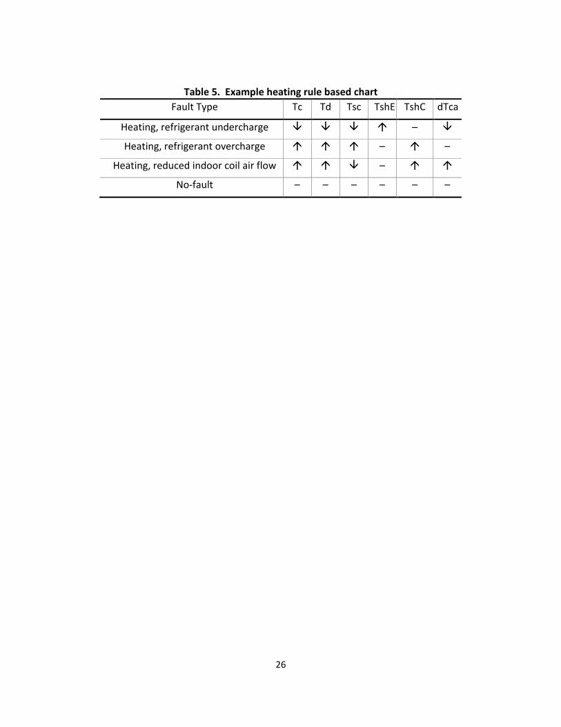
Examples of a rule based charts (RBC) are shown in Tables 4 and 5 for the cooling and heating modes, respectively. Each fault, listed by rows in the table, is characterized by positive, negative, or neutral temperature differences (cells in the corresponding fault row) for the important features (columns of the table). Each cell can be positive, negative or neutral and has an associated probability (0< P(C | X)<1). The probability of no-fault must also be included and determined in the same way as other faults. Obviously, a no-fault case occurs when the temperature differences are all neutral. The probability of a given fault is the product of all probabilities in a given row. When the probability of a given fault is higher than the no-fault probability, the system most likely has this fault occurring.
Table 4. Example cooling rule based chart Fault Type Te Tsh Tc Td Tsc dTea dTca
Cooling, refrigerant undercharge
Cooling, refrigerant overcharge – – – –
Cooling, reduced indoor coil air flow – – –
No-fault – – – – – – –
( )|↑ iP C X ( )|− iP C X ( )|↓ iP C X
µi µ ε+i iµ ε−i i xi
( )PDF ,i iµ σ
( )2,NF ,NF,i iN µ σ
,NFiµ
Moving Window Mean Value
No-Fault Reference Model Prediction
26
Table 5. Example heating rule based chart Fault Type Tc Td Tsc TshE TshC dTca
Heating, refrigerant undercharge –
Heating, refrigerant overcharge – –
Heating, reduced indoor coil air flow –
No-fault – – – – – –

27
References AHRI. (2004). Standard for performance rating of positive displacement refrigerant compressors
and compressor units. Arlington, VA: Air-Conditioning, Heating, and Refrigeration Institute.
Braun, J. (1999). Automated fault detection and diagnostics for vapor compression cooling equipment. International Journal of Heating, Ventilating, Air-Conditioning and Refrigerating Research, 5(2), 85-86.
Chen, B., & Braun, J. E. (2001). Simple rule-based methods for fault detection and diagnostics applied to packaged air conditioners. ASHRAE Transactions, 107(1), 847-857.
Kim, M., Payne, W., & Domanski, P. (2008). Cooling Mode Fault Detection and Diagnosis Method for a Residential Heat Pump. Gaithersburg, MD: NIST Special Publication 1087, National Inst. of Standards and Technology.
Kim, M., Yoon, S. H., Payne, W. V., & Domanski, P. A. (2008). Cooling mode fault detection and diagnosis method for a residential heat pump. Gaithersburg, MD: Special Publication 1087, National Inst. of Standards and Techn.
Kim, M., Yoon, S. H., Payne, W. V., & Domanski, P. A. (2010). Development of the reference model for a residential heat pump system for cooling mode fault detection and diagnosis. Journal of Mechanical Science and Technology, 24(7), 1481-89.
Payne, W., Domanski, P. A., & Hermes, C. (2006). Performance of a residential heat pump operating in the cooling mode with single faults imposed. NISTIR 7350, National Institute of Standards and Technology. Gaitherburg, MD: U.S. Dept. of Commerce.
Payne, W., Domanski, P. A., & Yoon, S. H. (2009). Heating mode performance measurements for a residential heat pump with single-faults imposed. Gaithersburg, MD: Technical Note 1648, National Inst. of Standards and Techn.
Rossi, T., & Braun, J. E. (1997). A statistical rule-based fault detection and diagnostic method for vapor compression air conditioners. HVAC&R Research, 3(1), 19-37.
Yoon, S. H., Payne, W. V., & Domanski, P. A. (2011). Residential heat pump heating performance with single faults imposed. Applied Thermal Engineering, 31, 765-771.

28
Acknowledgements The authors would like to acknowledge Min Sung Kim, Seok Ho Yoon, and Jin Min Cho for their work in developing the background material used in this user’s manual. Also, John Wamsley, Glen Glaeser, and Art Ellison provided technician support for the data used to develop the generic, no-fault reference temperature correlations.