FARM PRODUCTIVITY AND RURAL POVERTY IN INDIA

Gaurav Datt and Martin Ravallion

FCND DISCUSSION PAPER NO. 42

Food Consumption and Nutrition Division

International Food Policy Research Institute1200 Seventeenth Street, N.W.

Washington, D.C. 20036–3006 U.S.A.(202) 862–5600

Fax: (202) 467–4439

March 1998

FCND Discussion Papers contain preliminary material and research results, and are circulated prior to a fullpeer review in order to stimulate discussion and critical comment. It is expected that most Discussion Paperswill eventually be published in some other form, and that their content may also be revised.

ABSTRACT

To what extent do India’s rural poor share in agricultural growth? Combining data

from 24 household sample surveys spanning 35 years with other sources, we estimate a

model of the joint determination of consumption-poverty measures, agricultural wages,

and food prices. We find that higher farm productivity brought both absolute and relative

gains to poor rural households. A large share of the gains were via wages and prices,

though these effects took time. The benefits to the poor were not confined to those near

the poverty line.

CONTENTS

Acknowledgments . . . . . . . . . . . . . . . . . . . . . . . . . . . . . . . . . . . . . . . . . . . . . . . . . . . . iv

1. Introduction . . . . . . . . . . . . . . . . . . . . . . . . . . . . . . . . . . . . . . . . . . . . . . . . . . . . . . . 1

2. Model . . . . . . . . . . . . . . . . . . . . . . . . . . . . . . . . . . . . . . . . . . . . . . . . . . . . . . . . . . . . 5

3. Estimates . . . . . . . . . . . . . . . . . . . . . . . . . . . . . . . . . . . . . . . . . . . . . . . . . . . . . . . . . 9

Data . . . . . . . . . . . . . . . . . . . . . . . . . . . . . . . . . . . . . . . . . . . . . . . . . . . . . . . . . . . 9Results . . . . . . . . . . . . . . . . . . . . . . . . . . . . . . . . . . . . . . . . . . . . . . . . . . . . . . . . 12

4. Implications . . . . . . . . . . . . . . . . . . . . . . . . . . . . . . . . . . . . . . . . . . . . . . . . . . . . . . 18

Elasticities of Rural Poverty to Farm Yield . . . . . . . . . . . . . . . . . . . . . . . . . . . . . 19Why Are Elasticities Higher for Higher Values of "? . . . . . . . . . . . . . . . . . . . . . 21

5. Antecedents . . . . . . . . . . . . . . . . . . . . . . . . . . . . . . . . . . . . . . . . . . . . . . . . . . . . . . 22

6. Conclusions . . . . . . . . . . . . . . . . . . . . . . . . . . . . . . . . . . . . . . . . . . . . . . . . . . . . . . 32

Appendix . . . . . . . . . . . . . . . . . . . . . . . . . . . . . . . . . . . . . . . . . . . . . . . . . . . . . . . . . . . 34

References . . . . . . . . . . . . . . . . . . . . . . . . . . . . . . . . . . . . . . . . . . . . . . . . . . . . . . . . . . 38

TABLES

1. Annual growth rates . . . . . . . . . . . . . . . . . . . . . . . . . . . . . . . . . . . . . . . . . . . . . . 12

2. Regressions for rural poverty measures . . . . . . . . . . . . . . . . . . . . . . . . . . . . . . . 12

3. Regressions for the real wage rate and relative price of food . . . . . . . . . . . . . . . 17

4. Elasticities of rural poverty to average farm yield . . . . . . . . . . . . . . . . . . . . . . . . 21

FIGURE

1. Squared poverty gap and average farm yield, rural India 1959-94 . . . . . . . . . . . . 11

ACKNOWLEDGMENTS

These are the views of the authors, and should not be attributed to their employers.

The support of the World Bank's Research Committee (under RPO 677–82) is gratefully

acknowledged. The authors are also grateful to Berk Özler for help in setting up the data

set used here. For their comments, the authors thank Kaushik Basu, James Boyce, Jean

Drèze, Peter Lanjouw, Michael Lipton, Abhijit Sen, Lyn Squire, Anand Swamy,

Dominique van de Walle, Michael Walton, the Journal’s referees and seminar participants

at Cornell University, IFPRI, Harvard University, and the World Bank.

Gaurav DattInternational Food Policy Research Institute

Martin RavallionWorld Bank

Recent surveys spanning the wide range of views concerning the impacts of growth in farm1

productivity on rural poverty include Saith (1990), Singh (1990), and Lipton and Ravallion (1995).

1. INTRODUCTION

The following questions have been asked repeatedly in development research and

policymaking over many decades:

• How much do poor rural people share in the gains from higher average

productivity in agriculture? This has been the subject of (often vociferous)

debates. Contrast, for example, Ahluwalia's (1978, 320) conclusion that "there is1

evidence of some trickle down associated with agricultural growth" with Saith's

(1981, 205) claim that "there can be little doubt that current growth processes have

served as generators of poverty." One might imagine that these two authors were

talking about different places or times; but both were using data for the same

country—India—over roughly the same period (1957–73). The debate continues;

in more recent literature on India, one finds claims that "rapid agricultural growth

has benefitted all classes of the poor" (Singh 1990) and "acceleration in agricultural

growth by itself is unlikely to make a dent in rural poverty" (Gaiha 1995, 285).

• Does the relative position of poor people improve or worsen with agricultural

growth? This question has received less attention in the literature, but is

2

For a survey of various models of rural labor markets in this setting, see Drèze and Mukherjee (1989).2

Examples of the models we refer to include Osmani (1991), Mukherjee and Ray (1992), and Datt (1996).

Contrast, for example, the IFAD (1992) report with the World Bank (1990). The former emphasizes3

the scope for reducing rural poverty by developing smallholder agriculture, and pays rather little attention tothe role of the unskilled labor market; by contrast, the World Bank’s report emphasizes the importance ofpositive employment and wage effects in achieving pro-poor growth.

increasingly being asked. It is possible for the poorest to lose relatively, while

gaining absolutely; this is one interpretation of the idea of "trickle down." And it is

possible for a growth process to have sufficiently adverse effects on inequality that

absolute poverty increases. By contrast, some growth processes can entail

favorable distributional shifts, and, consequently larger gains to the poor than

suggested by a mere "trickle down."

• What role does the labor market play? Early development theories assumed a

rural economy in which extra employment would have no effect on the real wage

(Lewis 1954; Ranis and Fei 1961). By this view, the rural sector has a large labor

surplus and so there is little scope for the poor to gain via real wages. However,

other models of the rural labor market allow a labor surplus to coexist with a

process of wage determination in which labor-augmenting technical progress can

lead to higher real wages. Marked differences in the emphasis given to the role of2

the labor market can also be found in policy-oriented discussions. 3

• What role do food markets play? The food economy of India was largely closed

to external trade over the post-Independence period. Higher farm output is then

very likely to reduce the relative price of food, though this effect will no doubt be

3

See Ravallion (1991) (for Bangladesh) and Ravallion and van de Walle (1991) (for Java, Indonesia).4

See the results of Boyce and Ravallion (1991) for Bangladesh.5

buffered to some extent by governmental procurement and storage policies. At the

same time, the poorest in rural areas tend to be net consumers of food, in that they

have insufficient land for their own consumption needs. So, to the extent that

higher farm yields put downward pressure on food prices, the poorest will gain.

Against this, there may be poor net producers of food who lose. Heterogeneous

impacts among the poor of food price changes have been found in similar settings,4

though in most of South Asia, the general presumption is that the poorest in rural

areas will tend to gain from higher food output and, hence, lower food prices.

• Are there significant lags in the process through which poor people gain, or

lose, from agricultural growth? The dynamics of the distributional impacts of

growth are of obvious interest, though the topic has received surprisingly little

attention. Past models have analyzed consumption-based poverty measures within a

purely static framework. Yet labor markets are often found to exhibit short-run

stickiness in wages, and there is some evidence that this is also true in agricultural

labor markets in similar settings. Food markets, too, in this setting may generate5

price stickiness; for example, governmental intervention in food markets, through

producer price setting and storage, can no doubt buffer the effects of food prices

somewhat. Stickiness in wage and price adjustment to higher farm yields suggests

that long-run responses of poverty measures can exceed the short-run responses.

4

Addressing these questions empirically calls for a time series of representative

household-level surveys; yet such surveys are sporadic, at best, for most countries and

their comparability over time is often questionable. India is an exception. There one can

trace impacts on poverty over a long period, using reasonably comparable (at least by the

standards of international comparisons) and nationally representative surveys of

consumption.

This paper tests how much India's rural poor have benefitted from gains in average

farm productivity, what role labor and food markets have played, and whether the impacts

were distributionally biased one way or another. In the process, we try to resolve some

long-standing debates in the literature. Some new methods are brought to bear on these

questions. But, probably more important, some new data are used. Much of the scholarly

debate for India has focused (often—though not always—for lack of data) on periods of

rather little growth; these data may have low power in testing the effects of growth on

poverty. A new data set embracing a period of higher agricultural growth is used here.

The following section describes our structural model. Section 3 presents our

results. Some implications are discussed in Section 4. In Section 5, we compare our

results with those of related studies in the literature. Our conclusions can be found in

Section 6.

C ' C(W,R,Y,X,0) ,

5

(1)

2. MODEL

The bulk of the poor in rural India live on small farms with inadequate land for their

own food needs, or are landless. They depend heavily on earnings from supplying

unskilled wage labor to other farm or nonfarm enterprises. There are then two main

channels through which the poor might benefit from higher farm productivity generally.

One is by directly participating in the productivity gains, by producing more on their own

land, or finding more employment, either on someone else’s land or in some nonfarm

enterprise made possible by higher farm yields. These gains can be expected at given

wages and prices. The second potential channel is through higher wage rates, or lower

prices for consumed agricultural goods, notably food.

Our model incorporates both channels. We assume that individual consumption is a

function of the real wage rate for agricultural labor, the relative price of food, average

farm productivity, other exogenous aggregate variables, and the individual endowment of

land. (Standard micro-models can be used to justify such an assumption, so an elaboration

is not necessary here.) Individual consumption normalized by the poverty line is thus

given by

where W is the real wage rate, R is the relative price of food, Y is a measure of agricultural

productivity (such as yield per acre), X is a vector of other relevant variables (including,

0('0((W,R,Y,X) .

P"(W, R ,Y, X ) ' m0((W, R, Y, X )

0

(1 & C (W, R, Y, X, 0))" f (0)d0 ,

0

f (0)

0

0(

C( W, R, Y, X, 0() ' 1

6

One can also allow the distribution of land to be influenced by W and X. This would not change our6

estimated model.

(2)

(3)

for example, inflationary shocks), and is the amount of land owned (measured in units

of homogeneous quality), with interpersonal probability density, . The function C is

assumed to be strictly increasing in .

The poverty measure is defined on the distribution of consumption in a conventional

manner. The poverty level of landholding ( ) is obtained by inverting

to obtain

Using the Foster-Greer-Thorbecke (1984) class of poverty measures, we have6

where "" is a nonnegative parameter for the measure's aversion to inequality among the

poor. In the empirical work, we allow this parameter to take three possible values: "=0,

giving the head-count index; "=1, the poverty gap index; and "=2, the squared poverty

gap index. Only in the latter case does the measure penalize inequality among the poor.

We will also be interested in identifying any pro-poor effects on the distribution of

relative consumption, as distinct from absolute levels. For this purpose, we construct a set

of simulated poverty measures, in which the current poverty line is set at a constant

L ' L(W, R, Y, X, 0) ,

m4

0

L(W, R, Y, X, 0 ) f (0)d0 ' 0 ,

7

For example, one might also include measures in which the poverty line varies positively with the7

mean, but with an elasticity less than unity. For further discussion and references, see Ravallion (1994).

(4)

(5)

proportion of the current survey mean. The poverty measures are thus purged of the

direct effect of growth in average consumption, leaving only the effect via changes in

relative consumption levels (Datt and Ravallion 1992). Such measures can also be

thought of as examples of “relative poverty” measures, which is what we will call them,

though recognizing that there are potentially many examples of such measures.7

Market clearing conditions can readily deliver a model in which the wage rate and

price of food are functions of Y and X. Consider the labor market. Analogously to

equation (1), the net labor supply function (labor hired out minus labor hired in) is

and we assume that the market clearing condition,

can be solved for the wage rate as a function of R, Y, and X. However, as noted above,

this is only one possible economic model that would deliver a wage rate that depends on

these variables. That could also be justified by (for example) a model of imperfect

competition.

8

This also has implications for the welfare effects of external trade liberalization when domestic food8

prices are below world prices; see Ravallion (1991) on Bangladesh.

A similar representation of the food market will deliver a relative price of food that

is a function of W, Y, and X. Using the food market clearing condition to eliminate the

food price from the wage equation, and labor market clearing to eliminate wages from the

food price equation, we end up with reduced form models giving both W and R as

functions of Y and X.

We do not assume that markets adjust instantaneously. Short-run stickiness is

common in formal sector wages, but it has also been observed in rural settings in which

there are no trade unions or binding minimum wage rates (Boyce and Ravallion 1991). In

poor rural economies, employers will resist wage increases at least initially, and tacit

collusion or other forms of resistance on the supply side could also yield downward

stickiness. Long-run wage responses to agricultural growth can thus exceed short-run

responses. So we take it that our economic assumptions describe the steady-state8

equilibrium, but that observed current wages and food prices can deviate from that

equilibrium. We assume a first-order autoregressive process of adjustment to a new

equilibrium. Finally we assume that all these relationships can be adequately approximated

by an econometric model that is linear in logarithms.

Combining these assumptions, we estimate the following triangular system for the

observed data:

lnP"t ' $"0 % $"2lnW t% $"3lnRt% $"4lnYt % $)

"5X t % ,"t

lnWt ' (0 % (1lnWt&1 % (2lnRt&1 % (3lnYt % ()

4 X t % <Wt

lnRt ' B0 % B1lnRt&1 % B2lnWt&1 % B3lnYt % B)

4 X t % <Rt ,

$"i (i

,"t, <W

t, and <R

t

$"4

(3

9

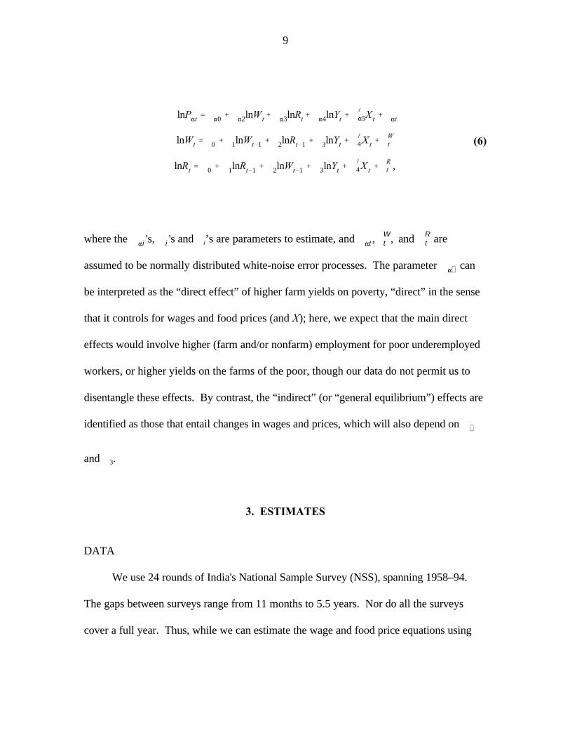
(6)

where the 's, 's and B ’s are parameters to estimate, and arei

assumed to be normally distributed white-noise error processes. The parameter can

be interpreted as the “direct effect” of higher farm yields on poverty, “direct” in the sense

that it controls for wages and food prices (and X); here, we expect that the main direct

effects would involve higher (farm and/or nonfarm) employment for poor underemployed

workers, or higher yields on the farms of the poor, though our data do not permit us to

disentangle these effects. By contrast, the “indirect” (or “general equilibrium”) effects are

identified as those that entail changes in wages and prices, which will also depend on

and B .3

3. ESTIMATES

DATA

We use 24 rounds of India's National Sample Survey (NSS), spanning 1958–94.

The gaps between surveys range from 11 months to 5.5 years. Nor do all the surveys

cover a full year. Thus, while we can estimate the wage and food price equations using

10

annual data, giving 35 observations, we can only estimate the poverty regressions on 24

observations.

We calculate poverty measures based on distributions of household consumption

expenditure (including from own production) per person. The poverty line is the one

recommended by the Planning Commission’s Expert Group (India 1993), and is set at a

per capita monthly expenditure of Rs 49 at October 1973–June 1974 all-India rural prices.

For the relative poverty measures, we fix mean consumption for each date at the overall

mean for the whole period; this is equivalent to setting the poverty line for each date at a

constant proportion of the mean for that date (specifically 83 percent of the mean). This

purges the poverty measures of all effects of changes in mean consumption, leaving only

distributional effects. However, since we are using a fixed-weight (Laspeyres) price index,

we will not pick up substitution effects on the demand side, but only income effects.

We measure average farm yield (Y) by agricultural output per acre of net sown area,

output being measured by a value-weighted quantity index of production of all crops.

(We comment further on this choice in Section 5.) The wage data are for male agricultural

wages. The price deflator for both the poverty line and wages is the Consumer Price

Index for Agricultural Laborers (CPI), corrected for inflation and firewood prices (see

Appendix for details). The index of the relative price of food was obtained by dividing the

food component of the CPI by the value of the general index.

The appendix describes how we mapped the annual data on other variables into the

NSS survey periods, and further details on data sources.

11

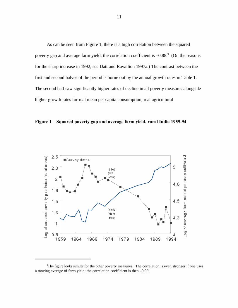
The figure looks similar for the other poverty measures. The correlation is even stronger if one uses9

a moving average of farm yield; the correlation coefficient is then –0.90.

As can be seen from Figure 1, there is a high correlation between the squared

poverty gap and average farm yield; the correlation coefficient is –0.88. (On the reasons9

for the sharp increase in 1992, see Datt and Ravallion 1997a.) The contrast between the

first and second halves of the period is borne out by the annual growth rates in Table 1.

The second half saw significantly higher rates of decline in all poverty measures alongside

higher growth rates for real mean per capita consumption, real agricultural

Figure 1—Squared poverty gap and average farm yield, rural India 1959-94

12

Table 1—Annual growth rates

Average annual rate of growth (%)1958–75 1976–94

Head-count index of poverty 1.18 –1.91Poverty gap index 1.42 –3.65Squared poverty gap index 1.65 –4.97Mean real consumption per person –0.93 1.76Real agricultural wage rate 0.33 2.84Agricultural output per acre of net sown area 1.51 2.91Net sown area per person in rural areas –1.53 –1.76Agricultural output per head of rural population –0.01 1.15Consumer price index for agricultural laborers 7.17 8.11Consumer price index for food 7.79 7.96Head-count index (relative) –0.49 –0.05Poverty gap index (relative) –1.07 –0.86Squared poverty gap index (relative) –1.45 –1.56

wages, agricultural yield, and nonagricultural output per person. In what follows, we try

to sort out the relative importance of these factors.

RESULTS

In estimating equation (6), the X vector comprised the net sown area per head of

rural population, the consumer price index for agricultural laborers for all commodities

(CPI), and a time trend. All variables except the time trend were measured in natural

Xi t&1 ' (1& (1/Jt ))Xit % (1/Jt )Xi t&Jt

13

The lagged values refer to values a year before the mid-point of the current survey period, and are10

estimated by interpolation using (and similarly for other lagged variables),

where J is the time between the midpoints of survey periods. We resort to interpolation because the NSSsurvey periods do not coincide with the annual periodicity of the time-dependent variables, which are thusnot centered at the mid-point of the survey periods.

logarithms. Both the current and lagged values of W, R, Y, and X were included, with up

to two year lags in Y.10

Starting with this unrestricted specification, we were led to a restricted form for

each poverty regression with just three explanatory variables, agricultural output per unit

net sown area, the real wage rate, and the relative price of food. Both current and lagged

values of yield and wages were retained. And the coefficients on both real wages and the

agricultural yield variables were not significantly different from each other for any of the

poverty measures, and so we imposed the restriction that they had the same coefficient.

Thus, in addition to the relative price of food, the data suggest that a key explanatory

variable is the (log of the) product of the real wage rate in agriculture and agricultural

output per acre. One can interpret this variable as the product of average labor

productivity in agriculture (output per worker) and agricultural labor earnings per acre, a

measure of labor intensive in agriculture. We shall call this variable “wage-weighted farm

yield.”

Thus we are drawn to a model in which the poverty measures are determined by the

productivity of labor in agriculture weighted by a measure of wage labor intensity, and the

relative price of food. The estimates of this model are given in Table 2. We subjected all

the regressions to a battery of standard residual diagnostic tests (serial correlation,

14

normality, heteroscedasticity) and the model passed all tests at the 5 percent level or

better. All parameter restrictions imposed on the initial model were tested and passed.

We also estimated the model, treating both the current year's wage and yield as

endogenous, and using lagged values up to two years and a time trend as instrumental

variables. The results were very similar.

Our results in Table 2 indicate that both higher agricultural wages and higher yields

reduce rural poverty, and that they do so with about the same elasticity. It is higher yields

combined with higher wages that matter.

There is also an independent adverse effect of higher food prices. The elasticities to

food price are high, though the relative price of food varied little over the period (in Table

1, note that the growth rates for the food price index are very close to those of the general

index.) The elasticities tend to be higher as the value of " is higher, i.e., the more

“distribution-sensitive” is the poverty measure.

15

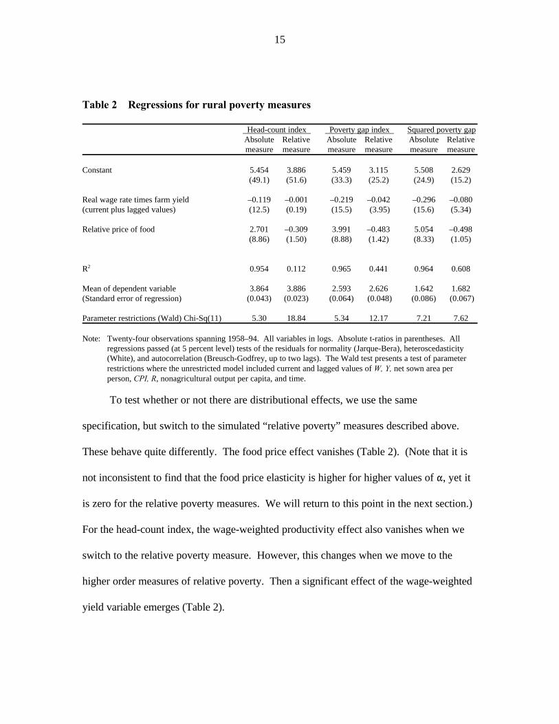
Table 2—Regressions for rural poverty measures

Head-count index Poverty gap index Squared poverty gapAbsolute Relative Absolute Relative Absolute Relativemeasure measure measure measure measure measure

Constant 5.454 3.886 5.459 3.115 5.508 2.629(49.1) (51.6) (33.3) (25.2) (24.9) (15.2)

Real wage rate times farm yield –0.119 –0.001 –0.219 –0.042 –0.296 –0.080(current plus lagged values) (12.5) (0.19) (15.5) (3.95) (15.6) (5.34)

Relative price of food 2.701 –0.309 3.991 –0.483 5.054 –0.498(8.86) (1.50) (8.88) (1.42) (8.33) (1.05)

R 0.954 0.112 0.965 0.441 0.964 0.6082

Mean of dependent variable 3.864 3.886 2.593 2.626 1.642 1.682(Standard error of regression) (0.043) (0.023) (0.064) (0.048) (0.086) (0.067)

Parameter restrictions (Wald) Chi-Sq(11) 5.30 18.84 5.34 12.17 7.21 7.62

Note: Twenty-four observations spanning 1958–94. All variables in logs. Absolute t-ratios in parentheses. Allregressions passed (at 5 percent level) tests of the residuals for normality (Jarque-Bera), heteroscedasticity(White), and autocorrelation (Breusch-Godfrey, up to two lags). The Wald test presents a test of parameterrestrictions where the unrestricted model included current and lagged values of W, Y, net sown area perperson, CPI, R, nonagricultural output per capita, and time.

To test whether or not there are distributional effects, we use the same

specification, but switch to the simulated “relative poverty” measures described above.

These behave quite differently. The food price effect vanishes (Table 2). (Note that it is

not inconsistent to find that the food price elasticity is higher for higher values of ", yet it

is zero for the relative poverty measures. We will return to this point in the next section.)

For the head-count index, the wage-weighted productivity effect also vanishes when we

switch to the relative poverty measure. However, this changes when we move to the

higher order measures of relative poverty. Then a significant effect of the wage-weighted

yield variable emerges (Table 2).

16

Is there also evidence of an effect of agricultural yields via the real wage rate?

Turning to the wage equation in (6), we began with the same variables for X as in the

poverty regressions, though now we can add the extra observations possible by using

annual data. The restriction that the coefficients on the current and lagged (log) price

level add up to zero was very comfortably accepted, so the inflation rate was used instead.

However, aside from the lagged real wage and the inflation rate, no other variables in X

were individually significant. Nor was the lagged food price significant. There was,

however, a significant loss of fit when all were dropped. Yet log farm yield per acre was

significant when the others were dropped. The restriction that the coefficients on current

and lagged lnY were equal passed easily. Table 3 gives the ordinary least squares (OLS)

estimate; an IV estimate using only lagged values instrumental variables gave very similar

coefficients and only slightly higher standard errors. The regression passed the same set

17

As an aside, it may be noted that one can also write our wage determination model in terms of first11

differences, augmented with an error correction term. The variables of interest—the logs of W, CPI, andY—all had unit roots (using Augmented Dickey-Fuller tests). Regressing the log wage on the other twovariables in levels, the residuals were found to be stationary, consistent with cointegration. However, theparameter restriction needed to yield the same model as in Table 3 performed very well.

Table 3—Regressions for the real wage rate and relative price of food

Wage rate Food price

Constant –0.641 0.060(4.04) (3.096)

Lagged dependent variable 0.763 0.890(10.85) (21.118)

Farm yield variable 0.117 –0.016a

(4.24) (3.791)

Inflation rate –0.641 0.135(9.46) (9.981)

R 0.980 0.9552

Mean of dependent variable 1.554 –0.048(Standard error of regression) (0.032) (0.006)

Note: Thirty-five annual observations, 1958–93. Absolute t-ratios in parentheses. All variables in logs. All regressions passed (at 5 percent level) tests of the residuals for normality (Jarque-Bera),heteroscedasticity (White), and autocorrelation (Breusch-Godfrey, up to two lags).

For the wage equation, the farm yield variable is the sum of current and lagged output per acre. For thea

food price equation, it is current output per acre plus the lagged first difference of output per acre.

of residual diagnostic tests described above, as well as a Wald test for omitted variables

(including the lagged food price and the full set of original variables in X). 11

The dynamic effect in the wage equation is strong, and there is also a sizable short-

run effect of inflation. The short-run farm-yield elasticity of the real wage is about 0.12,

18

rising to over eight times that figure in the long run. Thus, while we do find strong

support for real wage sluggishness, there is a detectable, though small, short-run impact of

current yield.

Are there also effects via food prices? Starting with the same set of X variables, and

following the same model selection and testing procedure, we were drawn to the model in

Table 2, with just two explanatory variables (in addition to the lagged food price), namely

the sum of current agricultural yield and its lagged first difference, and the rate of inflation.

The former variable is suggestive of an effect of yield on aggregate food supply (with

lagged effects through storage behavior); the elasticity is, however, very small (probably

reflecting governmental efforts to buffer food prices from shocks to farm output). There

is also a significant positive effect of inflation on the relative price of food. This could

well be due to an effect of the current agricultural wage on the relative price of food

(recalling that we have solved out the current wage rate). There is a potential concern

about endogeneity here, since the CPI appears on both sides of the equation. We also

estimated the same equation treating the current level of the CPI as endogenous, using its

lagged values over two years as an instrument. The results were very similar to Table 3;

the coefficient of the inflation rate was slightly higher (0.147) and remained highly

significant (a t-ratio of 4.97), while other coefficients and standard errors were almost

unaffected.

19

Given the difference in the data sets used, there is no straightforward test for common omitted12

variables between the poverty regressions and either of the wage and price equations.

We also checked for a common omitted variable determining both real wages and

food prices, by testing for a correlation between the residuals of the two equations.12

There was no sign of a common omitted variable; the correlation coefficient between the

residuals was 0.12.

4. IMPLICATIONS

The above results suggest that India’s poor gained)both absolutely and

relatively)from both higher agricultural wages and higher average farm yields, and with the

same elasticity. Lower food prices also helped. There is evidence of an effect of higher

farm yields on both the wage rate and food price. This section will examine the

implications of these results for understanding the total effect of agricultural growth on

rural poverty.

ELASTICITIES OF RURAL POVERTY TO FARM YIELD

Since agricultural wages and food prices do not adjust instantaneously to yield

gains, short-run responses of the poverty measures will differ from long-run responses.

The short-run (contemporaneous) elasticity of the poverty measure to a change in yield is

given by

MlnP"t

MlnYt

' $"2(3 % $"3B3 % $"4 .

MlnP (

"

MlnY ('

2$"2(3

(1 & (1)%

$"3B3

(1 & B1)% 2$"4 .

20

This formulae assumes that ( = B =0, which was accepted as a parameter restriction on (6). Notice132 2

also that it is the sum of the current and lagged ln Y on the right-hand side of both the poverty and wageregressions. Thus, one collects two terms in ln Y in the steady-state.

(7)

(8)

We shall refer to the last term on the right-hand side (RHS) as the “direct effect,” while

the first two terms are the “indirect effects,” via real wages and relative food prices,

respectively. Using "*" to denote steady-state values, the long-run elasticity of the

poverty measure to yield is 13

Again, the first two terms on the RHS are the cumulative indirect effects operating

through the wage rate and food prices, respectively, while the last term is the direct effect.

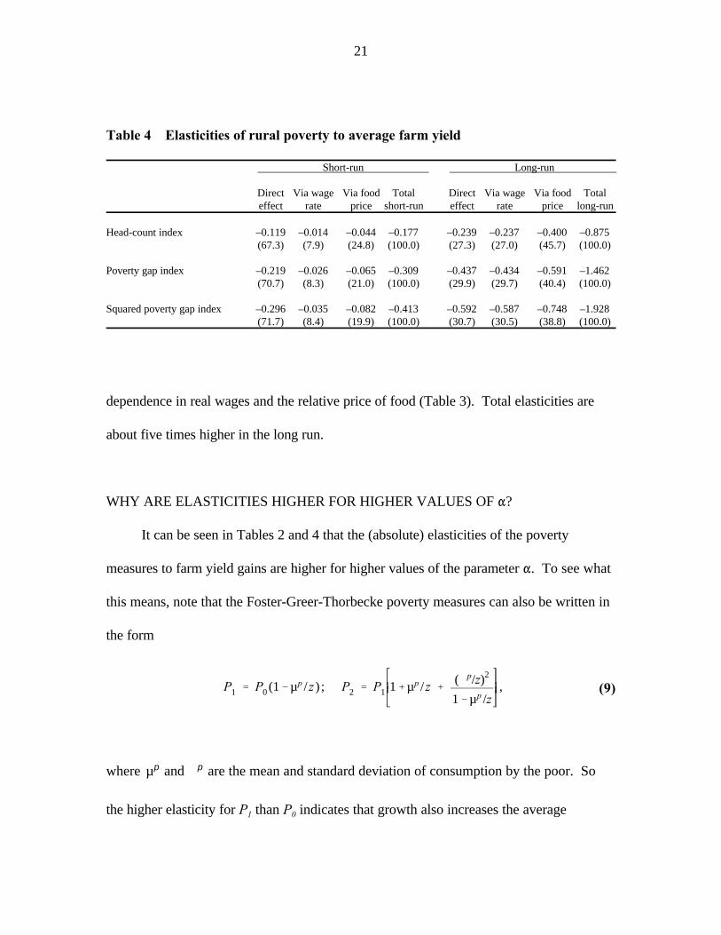
Table 4 gives the elasticities implied by our parameter estimates from Tables 2 and

3. In the short run, the indirect effect via the real wage is small, and dominated by other

channels, particularly the direct effect. But in the long run, the wage effects account for

about 30 percent of the total elasticity. The indirect effect via the relative price of food is

even higher. So the direct effect dominates in the short run, while the indirect effects via

wages and prices dominate in the long run. This reflects, in part, the high degree of serial

P1 ' P0 (1&µp /z ) ; P2 ' P1 1%µp /z %(Fp/z)2

1&µp /z,

µp Fp

21

(9)

Table 4—Elasticities of rural poverty to average farm yield

Short-run Long-run

Direct Via wage Via food Total Direct Via wage Via food Totaleffect rate price short-run effect rate price long-run

Head-count index –0.119 –0.014 –0.044 –0.177 –0.239 –0.237 –0.400 –0.875(67.3) (7.9) (24.8) (100.0) (27.3) (27.0) (45.7) (100.0)

Poverty gap index –0.219 –0.026 –0.065 –0.309 –0.437 –0.434 –0.591 –1.462(70.7) (8.3) (21.0) (100.0) (29.9) (29.7) (40.4) (100.0)

Squared poverty gap index –0.296 –0.035 –0.082 –0.413 –0.592 –0.587 –0.748 –1.928(71.7) (8.4) (19.9) (100.0) (30.7) (30.5) (38.8) (100.0)

dependence in real wages and the relative price of food (Table 3). Total elasticities are

about five times higher in the long run.

WHY ARE ELASTICITIES HIGHER FOR HIGHER VALUES OF "?

It can be seen in Tables 2 and 4 that the (absolute) elasticities of the poverty

measures to farm yield gains are higher for higher values of the parameter ". To see what

this means, note that the Foster-Greer-Thorbecke poverty measures can also be written in

the form

where and are the mean and standard deviation of consumption by the poor. So

the higher elasticity for P than P indicates that growth also increases the average1 0

µp Fp

1 & µp / z

Fp / µp

22

Since is increasing with yield, a higher elasticity for P than P must imply that is falling.142 1

When all consumptions grow at the same rate, it can be shown that the necessary and sufficient15

condition for the absolute elasticity of P to the mean to be greater than that of P is that f(z)/P < /z where1 0 0 µg

f(z) is the density of consumption at the poverty line z.

consumption of the poor ( falls). Furthermore, inequality among the poor—as

measured by the CV ( )—must be decreasing as average farm productivity

increases. Thus, with growth, there is also an improvement in distribution among the14

(changing number of) poor. Note too that although we do find significant yield and wage

effects on relative poverty, overall distribution neutrality (in that relative poverty measures

are unchanged) is not inconsistent with higher impacts on absolute poverty as " rises. For

example, all consumption levels could increase at the same rate while the mean

consumption of those below the poverty line also rises; whether it does or not depends on

the density of consumptions in a neighborhood of the poverty line. 15

5. ANTECEDENTS

Much of the scholarly debate on agricultural growth and rural poverty in India

started with a seminal paper by Ahluwalia (1978), who regressed measures of rural

poverty from 12 surveys between 1957 and 1974 against agricultural output per head of

the rural population and a time trend. He found that higher output was associated with

lower poverty, and that there was no trend independently of this. Subsequent papers

questioned (among other things) sensitivity to changes in the period of analysis (Griffin

23

Bell and Rich used an earlier version of our data set, rather than Ahluwalia's, and they made some16

changes to Ahluwalia's specification, as discussed below.

and Ghose 1979; Saith 1981). Ahluwalia (1985) and Bell and Rich (1994) returned to the

Ahluwalia regressions, adding data for another year (1977/78), and broadly confirmed his

conclusions.16

With so few observations, and relatively little sustained agricultural growth over the

period, the Ahluwalia series was clearly not ideal for this purpose (Srinivasan 1985). Our

doubling of the number of observations over the original Ahluwalia series, and the

substantial growth that has occurred since the late 1970s, has allowed us a more powerful

test for the effects of agricultural growth on rural poverty.

Higher-order poverty measures—reflecting distribution below the poverty

line—have often been used in the literature, though their role has been rather incidental.

Ahluwalia (1978, 1985) and others included the Sen (1976) index, but did not draw out

implications concerning the depth of impacts on the poor. Our results indicate differences

in the impact of agricultural growth between different measures, arising from changes in

distribution below the poverty line. We find no support for claims that productivity gains

in Indian agriculture by-passed the poorest.

Past work has not tested for pro-poor distributional effects (which, as we have

noted, is a different thing to testing impacts on higher-order poverty measures). Our

approach, using simulated measures to isolate distributional shifts, has an antecedent in the

method used by Datt and Ravallion (1992) to decompose changes in poverty into growth

24

and redistribution components. We cannot explain the distributional component of the

head-count index, but we do find that wages and yields can help explain the distributional

components of the higher order measures. Higher wages and yields entail an improved

distribution from the point of view of poverty, although the bulk of their effect (in terms of

the elasticities in Table 2) is clearly through the growth component.

Turning to the explanatory variables, past studies have followed Ahluwalia in using

farm output per head rather than per acre, which we have used. The log of output per

person is simply the sum of the logs of output per acre and acres per person, and we

initially included both variables. The fact that we can reject the null that they have the

same coefficients means that farm output per person is not the relevant variable for

predicting poverty. Although output per person and output per acre are highly correlated

(the correlation coefficient is 0.89 over the 35 annual observations), the latter variable is

clearly the better predictor of how much the poor share in agricultural growth. In

interpreting this finding, it should be recalled that we do not have either farm or nonfarm

employment on the RHS (we return to this point). Controlling for wages and prices, it

may well be that yield per acre is the better predictor of the underlying employment effects

of agricultural growth; for example, one would expect it to better reflect the potential for

multiple cropping in a given year, a key determinant of the demand for agricultural labor.

Our finding that lagged output matters, and it has a similar effect as current output, echoes

Ahluwalia (1985).

25

In some cases, this was the log CPI (Narain), while in others it was the deviation from trend (Saith,17

Gaiha). But with the trend already included in the regression, this difference will only affect the interpretationof the time trend.

We have also added real wages. It is odd that the real agricultural wage rate has

not figured more prominently in this literature, given how much India's rural poor depend

on agricultural labor markets. Bardhan (1984, Chapter 14) found a significant poverty-

reducing effect of higher real agricultural wages in cross-sectional data for West Bengal.

We know of only one other study that looked at the impact of the real wage rate on the

evolution over time of rural poverty in India, namely van de Walle (1985), who used the

earlier Ahluwalia poverty measures for 1959–71. However, numerous observers have

conjectured that this is an important variable (including Acharya and Papanek 1992).

Since this is a very strong predictor in our results, it appears that this may have been an

important omitted variable in other studies.

The level of the nominal price index has figured prominently in past work. Saith

(1981), Narain (see Desai 1985) and others (Mathur 1985; Gaiha 1989) added the level of

the CPI to the original Ahluwalia (1978) model, and this sparked further debate. It is17

difficult to believe that a monetary variable such as this could have long-run real effects in

a correctly specified model (Bliss 1985). The price-level effect may well be picking up

other omitted income sources or financial assets that matter to the poor (agricultural labor

and services, or cash holdings) and are not fully indexed for price changes (Desai 1985;

Bliss 1985; Sen 1985). We suspect that the significant price level effect identified in the

literature reflects an omitted variable bias, the key omitted variable being the real wage

26

Bell and Rich (1994) find significant effects on the head-count index of their measure of the18

unanticipated component of inflation, though they do not include the real wage rate.

One can also find a highly significant, but spurious, effect of the relative price of food on real wages19

if one does not control for the rate of inflation.

rate. While we have allowed effects of price levels, this proved to be insignificant once the

real wage was added. (Notice also that we included current and lagged price levels in18

the Wald test for omitted variables reported in Table 2.)

However, we do find effects of inflation on poverty via wages and food prices. The

inflation rate (as distinct from the price level) also appears to be an important omitted

variable in past work on the determinants of rural poverty in this setting. For example, if

one reestimates our wage regression, dropping the rate of inflation and adding the log of

the CPI, then the latter has a significant negative coefficient (–0.17 with a t-ratio of 3.49);

yet this is clearly spurious, for as soon as one returns the rate of inflation to the same

regression, the effect of the price level vanishes (the coefficient drops to 0.04, with a t-

ratio of 0.93, while the inflation rate is highly significant (a coefficient of –0.70, with a t-

ratio of 7.49).19

We remain somewhat puzzled as to why there is such a strong adverse effect on the

poverty measures of higher food prices. Following the argument in the introduction, we

expected this to be a distributional effect. Our tests do not support that view (Table 2),

though data limitations (notably the use of a single fixed-weight deflator) entail that we

can only expect to pick up any distributional effects on the income side, leaving out any

effects via demand behavior. Nonetheless, mean rural consumption is strongly negatively

27

Sen (1996) presents regressions for the head-count index (using an earlier version of our data set that20

we provided) in which variables for “nonagricultural employment” and “commercialization” appear on theright-hand side. However, no information is supplied in his paper as to where these data come from, and noreply was received to our letter asking for sources. We assume that the nonagricultural employment serieswas created by some sort of interpolation. Substantial interpolation would have been required, given the sparseemployment data.

correlated with the relative price of food (the simple correlation coefficient over the 24

survey rounds is 0.82.) That is surprising, given that (in this largely closed food economy)

the rural sector as a whole produced more food than it consumed. However, it should be

noted that there was no significant trend over the whole period in the relative price of

food; its ability to help explain the poverty measures appears to be due to a correlation

with the fluctuations in poverty over time. The explanation may lie in common shocks to

food supply and/or savings behavior.

It has been argued that nonagricultural employment was also an important factor in

reducing rural poverty in India. Presumably this was to some extent the result of

agricultural growth (Hazell and Haggblade 1993), though it has also been argued that

there was an independent effect (Sen and Ghosh 1993; Sen 1996). Testing for an

independent effect of nonfarm employment is difficult, given that most NSS rounds did

not collect data on rural employment, and there is only sporadic data from other sources.20

We tested (current and lagged) nonagricultural net domestic product (urban plus rural) per

head of rural population as an additional explanatory variable for the absolute poverty

measures in Table 2, but it was insignificant and had little effect on other coefficients. We

repeated this test dropping the real agricultural wage rate from the poverty regressions, to

28

see if there is an indirect effect via wages; again, nonagricultural output per capita was

(highly) insignificant.

We have examined this issue further at the state level in India, and found that

deviations from trend in (state-specific) nonagricultural output do help explain the

fluctuations over time in the poverty measures. However, we find that differences

between states in the trend of nonagricultural output growth had no power to explain

differences in the trend rate of poverty reduction, once one controls for the trend rates of

farm yield growth and initial conditions related to physical and human infrastructure (Datt

and Ravallion 1997b).

Our analysis at the state level also allowed for an independent effect of government

spending, but did not find a reasonably significant effect on either the trend rates of

poverty reduction or deviations from trend (though the effect was mildly significant in the

latter case for the head-count index). However, we did find evidence of an indirect effect

via higher farm yields. To test this, Datt and Ravallion (1997b) regressed the agricultural

yield on the other explanatory variables in their model, including public spending at state

level. The latter had a significant positive impact; yield had an elasticity of 0.29 (t-

ratio=3.18). This suggests that state development spending has helped reduce rural

poverty through its impact on average farm yield. There could well have also been effects

via rural nonfarm employment; we did find significant effects on nonagricultural output.

However, we were also unable to reject the hypothesis that growth in agricultural yields

and nonagricultural output Granger-caused higher development spending; lagged

29

For a recent argument, see Sen and Ghosh (1993), although their own results do not appear to be21

conclusive on this point.

agricultural yield and nonagricultural output had significant positive effects on state

development spending. Further work is needed to disentangle these effects.

There has also been concern in India that the employment elasticity of agricultural

growth has been falling, and (hence, it is argued) that agricultural growth is now less

poverty reducing than it used to be. What do our data and models suggest? Although21

there is not a suitable time series of agricultural employment, we can directly test for a

trend decline in the farm-yield elasticity of our poverty measures. To do so, we added an

interaction effect between time (mid-point of the NSS round, in years) and the wage-

weighted farm yield variable (Table 2). The interaction effect was insignificant for all

three poverty measures, both absolute and relative. We do not find a trend decline in the

yield elasticity of rural poverty in India.

Aside from the specification of the RHS variables, studies in the literature have

differed in their assumptions (often implicit) about dynamics, and the properties of the

error term. Virtually all of the poverty regressions in this literature are static. The only

study to allow for serial dependence is Bell and Rich (1994). To deal with the uneven

spacing, they filled the gaps by two alternative methods: linear interpolation and a

forecasting model relating current poverty to its lagged value and current rainfall. They

did not use observations after 1977/78, being concerned about the gap to the next round

(1983). The shortage of surveys for estimating the poverty measures will entail a small-

30

The test allowed for uneven spacing by estimating the model under a common factor restriction. This22

is equivalent to estimating a static model with an AR1 error term, in which the usual autoregressioncoefficient is raised to the power of the elapsed time between surveys.

In an earlier working paper version (summarized in Ravallion and Datt 1996b), we had omitted the23

relative price of food from the poverty regressions, and so were drawn toward a dynamic specification.Comments on that working paper by Sen (1996) led us to test the effect of adding the relative food price. Note,however, that the conclusions we had drawn in Ravallion and Datt (1996b) about dynamic responses ofpoverty measures to agricultural growth remain valid, given the dynamic behavior of both food prices andwages in response to agricultural growth.

For example, Acharya and Papanek (1992) estimate models of agricultural wage determination for24

India using time series data, but do not allow for dynamic effects.

sample bias in dynamic models. We tested for an independent dynamic effect, by adding

the lagged poverty measure to the regressions in Table 2. This was insignificant. Note,22

however, that there are still dynamic effects via wages and prices in our model. We also

found that if we dropped the relative price of food from the right-hand side, then the

poverty regressions called for either a lagged dependent variable or an autoregression

(AR1) correction to the error term. Significant dynamics in a poverty regression that

excludes this variable can thus be attributed to omitted variable bias. 23

Serial dependence in wages and prices is more likely to be a structural feature,

reflecting stickiness in wage and price adjustment. Some past time series models of real

wage determination have been static. Omitting lagged wages in our model leads to24

substantial overestimation of the short-run effect of agricultural productivity on wages and

underestimation of the long-run elasticity, and (of course) the residuals were highly serially

dependent (a Durbin-Watson statistic of 0.77). Lal (1988) estimates a model for the real

agricultural wage in India as a function of agricultural output and land under cultivation.

Lal's short-run elasticity of wage to yield for 1958–78 is also considerably higher than

lnP0t ' 12.94 & 0.72(lnYPCt % lnYPCt&1 ) & 0.001 t(2.45) (3.95) (0.37) ,

lnP0 t ' 96.92 & 0.82lnYPCt % 0.57lnCPIt & 0.047 t(2.80) (2.73) (2.30) (2.54) .

YPC

31

The Durbin-Watson statistic is 0.76, and the Breush-Godfrey test with two lags indicates significant25

serial correlation at the 1 percent level.

(10)

(11)

ours. This appears to be due to a difference in specification. Lal differences all variables

in his model. The omission of an error-correction term (real wages and farm yields are

cointegrated in our data) entails that his model does not have a long-run solution, and it

appears to impart an upward bias on the short-run yield effect on wages.

It is of interest to see what a poverty regression consistent with the Ahluwalia

specification looks like on our new data. The Ahluwalia specification gives

where is agricultural output per capita. The R is 0.76, though there is clearly strong2

serial correlation in the error term, so that this R and the t-ratios are probably a poor2

guide to fit and significance. Notice that Ahluwalia’s specification gives a higher25

elasticity to agricultural output, namely –1.44, as compared to our long-run estimate of

–0.88 (Table 4). The main reason for this appears to be our use of output per acre rather

than output per person; when we rerun the Ahluwalia specification using our yield

variable, the long-run elasticity becomes –0.92 (t=5.24). The Narain-Saith specification

gives

32

The R is 0.69, though there is still significant positive serial correlation in the residuals. 2

An encompassing model can be used to jointly test our changes to both specifications. By

adding both (current and lagged) net sown area per person, price level, and relative price

of food to our preferred model in Table 2, we can do a nested test against the Ahluwalia-

Narain-Saith models. All three variables were highly insignificant (individually and

jointly); a Wald test gave a Chi-square of 1.14. Our model fits the data better.

6. CONCLUSIONS

We have estimated the effects of farm yield growth in rural India on various poverty

measures, real agricultural wages, and the relative price of food, using data spanning the

period 1958–94. We find that higher real wages and higher farm yields reduced absolute

poverty, and with about the same elasticity. A composite variable—wage earnings per

acre times average product per worker—has remarkably strong predictive power for

various measures of absolute poverty. When we turn, instead, to measure relative

poverty—by fixing the poverty line as a constant proportion of the current mean, we find

significant, but much smaller effects, below the poverty line. We also find that the poor

gained in absolute terms from lower relative prices of food. However, this effect is not

evident in measures of relative poverty. Our results suggest that the bulk, but not all, of

the gains to the poor from higher farm yields and higher real wages were via rising average

living standards rather than improved distribution. Even so, the gains to the poor from

higher average yields were not confined to those near the poverty line, but reached deeper.

33

We also find evidence of important indirect channels linking average farm

productivity to living standards of the rural poor. There is evidence that real agricultural

wages responded positively to higher farm yields, presumably through effects on labor

demand, such as due to multiple cropping. There is also a strong link through food prices.

While the impact of agricultural growth on food prices is quantitatively small, even small

food price changes can have large effects on absolute poverty. Inflation also had adverse

effects on the poor, via its short-term effect on real wages and the food prices.

Neither the real wage rate nor the price of food adjusted instantaneously to higher

yields. The combined effect of this wage and price stickiness is that the short-run gains to

poor people of higher farm productivity are far lower than the long-run gains. Indeed, the

short-run effects operating via wages and prices are minor compared to those through

other channels. But in the long run, the dynamic general equilibrium effects account for

about 70 percent of the steady-state elasticity of absolute poverty to a farm yield increase.

Overall elasticities in the long run are five times higher than the short-run values, and long-

run elasticities are about one for the head-count index of poverty, rising to about two for

the squared poverty gap index.

34

APPENDIX

DATA SOURCES

POVERTY MEASURES

The poverty measures are based on the published National Sample Survey (NSS)

data on distributions of per capita monthly expenditure. The distributions are available for

33 NSS rounds, starting with the 3rd round for August 1951–November 1951 and going

up to the 50th round for July 1993–June 1994. In keeping with data available on other

variables (see below), the poverty estimates used here are for a shorter period, from NSS

round 14 (July 1958–June 1959) to round 50 (July 1993–June 1994). The poverty line is

defined by a per capita monthly expenditure of Rs 49 in rural areas at October 1973–June

1974 prices. This poverty line was originally proposed by the Task Force on Projections

of Minimum Needs and Effective Consumption Demand (India 1979), and was later also

endorsed by the Expert Group on Estimation of Number and Proportion of Poor (India

1993). The deflator we have used to adjust for temporal changes in the cost of living in

the rural sector is the Consumer Price Index for Agricultural Laborers (CPI). Using the

formulae in Datt and Ravallion (1992), point estimates of poverty measures are calculated

using data on mean per capita consumption and the estimated parameters of fitted Lorenz

curves. Either the Beta Lorenz specification (Kakwani 1980) or the General Quadratic

specification (Villasenor and Arnold 1989) were used, depending on which fitted best;

both satisfied the theoretical conditions needed for a valid Lorenz curve in all survey

35

rounds. A complete series of the poverty measures can be found in Özler, Datt, and

Ravallion (1996), Datt (1997) and World Bank (1997).

THE PRICE INDICES

The CPI for agricultural laborers (CPIAL) for the period we cover is compiled from

the Labour Bureau's monthly series on consumer price indices (published in the Indian

Labour Journal and the Indian Labour Yearbook.) Beginning September 1964, the index

is directly available at the all-India level. For the earlier period, September 1956 through

August 1964, however, only state-level indices are available. We have aggregated these

into an all-India index using the same weighting diagram as used in the Labour Bureau

series for the later period.

A problem with this price index is that the Labour Bureau ignored increases in

firewood prices after 1960–61; firewood is typically a common property resource for

agricultural laborers, but it is also a market good, and so the Labour Bureau's practice is

questionable. (The NSS values firewood consumption from own-production at local

market prices. Also, see Minhas et al. 1987 for further discussion.) To deal with this

problem, we estimated a new deflator, replacing the firewood subseries by one based on

mean rural firewood prices (only available from 1970) and a series derived by assuming

that firewood prices increased at the same rate as all other items in the Fuel and Light

category (prior to 1970); see Datt (1997) for further discussion of this adjustment to the

CPIAL.

36

The index of the relative price of food is defined to be the ratio of the food

component of the CPIAL to the above (adjusted) CPIAL for all commodities.

AGRICULTURAL WAGES

Our data on nominal daily male agricultural wages are compiled from Jose (1974,

1988), supplemented with the data reported in the Report of the National Commission on

Rural Labour (Volume I) [India 1991], and Agricultural Wages in India reports since

1984–85. (A complete time series is not available for women.) The primary source of all

these data is the Ministry of Agriculture's annual publication, Agricultural Wages in India

(AWI). These data were aggregated to derive all-India wage rates using state- and year-

specific weights, as described in Özler et al. (1996).

AGRICULTURAL OUTPUT AND AREA

These data are collated from various issues of the publication, Area and Production

of Principal Crops in India, produced by the Ministry of Agriculture. The data are in the

form of three annual indices: (1) the index of agricultural production, which is a

Laspeyres quantity index of production of all crops, where the weight for a particular crop

is given by the average value of that crop's output over the triennium ending 1981–82.

(Alternatively, one can use value added in agriculture, though this makes little difference,

since it is highly correlated with output; the correlation coefficient is 0.97 in logs); (2) the

index of gross cropped area under all crops (including area sown more than once during

37

the year) with the same base period, i.e., the triennium ending 1981–82; (3) the index of

net sown area also with the same base period. All three indices refer to the agricultural

year from July to June.

POPULATION

Annual estimates of the rural population are constructed using census data from all

five censuses conducted in the post-independence period. Sectoral populations are

assumed to grow at a constant rate between censuses. The population estimates are

centered at the beginning of each calendar year that coincides with the mid-point of the

corresponding agricultural year.

MATCHING NON-NSS DATA WITH NSS ROUNDS

The data on the CPI are originally collated on a monthly basis and hence permit

easy aggregation in the form of averages over months for the corresponding NSS survey

periods. Population estimates were made for the mid-point of each NSS survey period.

However, data on the other variables are only available on an annual basis for each

agricultural year. For these variables, we have constructed values corresponding to a

given NSS round as (1) the value of the variable for the agricultural year if the survey

period coincides with (or falls entirely within) the agricultural year, or otherwise, as (2) a

weighted average of the values for agricultural years overlapping with the survey period of

that round.

38

REFERENCES

Acharya, S., and G. Papanek. 1992. Agricultural wages and poverty in India: A model of

rural labor markets. Tata Institute of Social Sciences, India. Photocopied.

Ahluwalia, M. S. 1978. Rural poverty and agricultural performance in India. Journal of

Development Studies 14 (3): 298–323.

Ahluwalia, M. S. 1985. Rural poverty, agricultural production, and prices: A

reexamination. In Agricultural change and rural poverty, ed. J. Mellor and G.

Desai. Baltimore, Md., U.S.A.: Johns Hopkins University Press.

Bardhan, P. 1984. Land, labor, and rural poverty. Essays in development economics

New York: Columbia University Press.

Bell, C., and R. Rich. 1994. Rural poverty and agricultural performance in post-

independence India. Oxford Bulletin of Economics and Statistics 56 (2): 111–133.

Bliss, C. 1985. A note on the price variable. In Agricultural change and rural poverty,

ed. J. Mellor and G. Desai. Baltimore, Md., U.S.A.: Johns Hopkins University

Press.

Boyce, J. K., and M. Ravallion. 1991. A dynamic econometric model of agricultural

wage determination in Bangladesh. Oxford Bulletin of Economics and Statistics 53

(4): 361–376.

Datt, G. 1996. Bargaining power, wages, and employment: An analysis of agricultural

labor markets in India. New Delhi: Sage Publications.

39

Datt, G. 1997. Poverty in India, 1951–1994: Trends and decompositions. International

Food Policy Research Institute, Washington, D.C. Photocopied.

Datt, G., and M. Ravallion. 1992. Growth and redistribution components of changes in

poverty measures: A decomposition with applications to Brazil and India in the

1980s. Journal of Development Economics 38 (2): 275–295.

Datt, G., and M. Ravallion. 1997a. Macroeconomic crises and poverty monitoring: A

case study for India. Review of Development Economics 1 (2): 135–152.

Datt, G., and M. Ravallion. 1997b. Why have some Indian States done better than others

at reducing rural poverty? Economica, Vol. 64 (in press).

Desai, G. M. 1985. Trends in rural poverty in India: An interpretation of Dharm Narain.

In Agricultural change and rural poverty, ed. J. Mellor and G. Desai. Baltimore,

Md., U.S.A.: Johns Hopkins University Press.

Drèze, J., and A. Mukherjee. 1989. Labor contracts in rural India: Theories and

evidence. In The balance between industry and agriculture in economic

development 3: Manpower and transfers, ed. S. Chakravarty. London: Macmillan.

Foster, J., J. Greer, and E. Thorbecke. 1984. A class of decomposable poverty measures.

Econometrica 52 (3): 761–765.

Gaiha, R. 1989. Poverty, agricultural production, and price fluctuations in rural India: A

reformulation. Cambridge Journal of Economics 13 (2): 333–352.

Gaiha, R. 1995. Does agricultural growth matter to poverty alleviation? Development

and Change 26 (2): 285–304.

40

Griffin, K. B., and A. K. Ghose. 1979. Growth and improverishment in the rural areas of

South Asia. World Development 7 (4/5): 361–384.

Hazell, P., and S. Haggblade. 1993. Farm-nonfarm growth linkages and the welfare of

the poor. In Including the poor, ed. M. Lipton and J. van der Gaag. Washington,

D.C.: World Bank.

IFAD (International Fund for Agricultural Development). 1992. The state of world rural

poverty: An enquiry into causes and consequences. New York: New York

University Press.

India. 1979. Report of the task force on projections of minimum needs and effective

consumption. New Delhi: Planning Commission, Government of India.

India. 1991. Report of the National Commission on Rural Labour: Volume 1. New

Delhi: Ministry of Labour, Government of India.

India. 1993. Report of the expert group on estimation of proportion and number of

poor. New Delhi: Planning Commission, Government of India.

Jose, A. V. 1974. Trends in real wage rates of agricultural laborers. Economic and

Political Weekly 9 (March 30): A25–A30.

Jose, A. V. 1988. Agricultural wages in India. Asian Employment Programme Working

Papers. New Delhi: Asian Regional Team for Employment Promotion (ARTEP),

International Labour Organization.

Kakwani, N. 1980. On a class of poverty measures. Econometrica 48 (2): 437–446.

41

Lal, D. 1988. Trends in real wages in rural India 1880–1980. In Rural poverty in South

Asia, ed. T. N. Srinivasan and P. K. Bardhan. Delhi: Oxford University Press.

Lewis, W. A. 1954. Economic development with unlimited supplies of labor.

Manchester School 22: 139–191.

Lipton, M., and M. Ravallion. 1995. Poverty and policy. In Handbook of development

economics, Vol. 3, ed. J. Behrman and T. N. Srinivasan. Amsterdam: North

Holland.

Mathur, S. C. 1985. Rural poverty and agricultural performance in India. Journal of

Development Studies 21 (3): 422–428.

Minhas, B. S., L. R. Jain, S. M. Kansal, and M. R. Saluja. 1987. On the choice of

appropriate consumer price indices and data sets for estimating the incidence of

poverty in India. Indian Economic Review 22 (1): 19–49.

Mukherjee, A., and D. Ray. 1992. Wages and involuntary unemployment in the slack

season of a village economy. Journal of Development Economics 37 (1/2):

227–264.

Osmani, S. R. 1991. Wage determination in rural labor markets. The theory of implicit

co-operation. Journal of Development Economics 34 (1): 3–23.

Özler, B., G. Datt, and M. Ravallion. 1996. A database on poverty and growth in India.

Development Research Group, World Bank, Washington, D.C.

Ranis, G., and J. Fei. 1961. A theory of economic development. American Economic

Review 56: 533–558.

42

Ravallion, M. 1991. Rural welfare effects of food price changes under induced wage

responses: Theory and evidence for Bangladesh. Oxford Economic Papers 42 (3):

574–585.

Ravallion, M. 1994. Poverty comparisons. Fundamentals in Pure and Applied

Economics, Volume 56. Chur, Switzerland: Harwood Academic Press.

Ravallion, M., and G. Datt. 1996a. How important to India's Poor is the sectoral

composition of growth? World Bank Economic Review 10 (1): 1–26.

Ravallion, M., and G. Datt. 1996b. India’s checkered history in the fight against poverty:

Are there lessons for the future? Economic and Political Weekly 31 (September):

2479–2486.

Ravallion, M., and D. van de Walle. 1991. The impact on poverty of food pricing

reforms: A welfare analysis for Indonesia. Journal of Policy Modeling 13 (2):

281–299.

Saith, A. 1981. Production, prices, and poverty in rural India. Journal of Development

Studies 19 (2): 196–214.

Saith, A. 1990. Development strategies and the rural poor. The Journal of Peasant

Studies 17: 171–244.

Sen, A. 1976. Poverty: An ordinal approach to measurement. Econometrica 44 (2):

219–231.

43

Sen, A. 1985. Dharm Narain on poverty: Concepts and broader issues. In Agricultural

change and rural poverty, ed. J. Mellor and G. Desai. Baltimore, Md., U.S.A.:

Johns Hopkins University Press.

Sen, A. 1996. Economic reforms, employment, and poverty: Trends and options.

Economic and Political Weekly 31 (September): 2459–2478.

Sen, A., and J. Ghosh. 1993. Trends in rural employment and the poverty-employment

linkage. Asian Regional Team for Employment Promotion, International Labour

Organization, New Delhi, India.

Singh, I. 1990. The great ascent. The rural poor in South Asia. Baltimore, Md.,

U.S.A.: Johns Hopkins University Press for the World Bank.

Srinivasan, T. N. 1985. Agricultural production, relative prices, entitlements, and

poverty. In Agricultural change and rural poverty, ed. J. Mellor and G. Desai.

Baltimore, Md., U.S.A.: Johns Hopkins University Press.

van de Walle, D. 1985. Population growth and poverty: Another look at the Indian time

series data. Journal of Development Studies 21 (3): 429–439.

Villasenor, J., and B. C. Arnold. 1989. Elliptical Lorenz Curves. Journal of

Econometrics 40 (2): 327–338.

World Bank. 1990. World development report: Poverty. New York: Oxford University

Press.

World Bank. 1997. India: Achievements and challenges in reducing poverty.

Washington, D.C.: World Bank.