Fault Detection in a Heat Exchanger, Comparative … · between Dynamic Principal Component Analysis ... Detección de Fallas en un ... Fault Detection in a Heat Exchanger, Comparative

Computación y Sistemas Vol. 14 No. 3, 2011, 269-282 ISSN 1405-5546

Fault Detection in a Heat Exchanger, Comparative Analysis between Dynamic Principal Component Analysis and Diagnostic

Observers

Detección de Fallas en un Intercambiador de Calor, Análisis Comparativo entre Análisis de Componentes Principales Dinámico y Observadores de Diagnóstic

Juan C. Tudón Martínez1, Rubén Morales Menéndez1, Ricardo A. Ramírez Mendoza1, Luis E. Garza Castañón1 and Adriana Vargas Martínez1

1Tecnológico de Monterrey, Campus Monterrey Monterrey N.L., México

{A00287756, rmm, ricardo.ramirez, legarza, A00777924}@itesm.mx

Article received on September 01, 2009; accepted on February 08, 2010

Abstract. A comparison between the Dynamic Principal Component Analysis (DPCA) method and a set of Diagnostic Observers (DO) under the same experimental data from a shell and tube industrial heat exchanger is presented. The comparative analysis shows the detection properties of both methods when sensors and/or actuators fail online, including scenarios with multiple faults. Similar metrics are defined for both methods: robustness, quick detection, isolability capacity, explanation facility, false alarm rates and multiple faults identifiability. Experimental results show the principal advantages and disadvantages of both methods. DO showed quicker detection for sensor and actuator faults with lower false alarm rate. Also, DO can isolate multiple faults. DPCA required a minor training effort; however, it can not identify two or more sequential faults. Keywords: Fault Detection and Diagnosis, Model Classification, Computer Application, Dynamic Principal Component Analysis, Diagnostic Observers. Resumen. El artículo presenta una comparación entre dos métodos de detección de fallas, Análisis de Componentes Principales Dinámico (DPCA por sus siglas en inglés) y Observadores de Diagnóstico (DO por sus siglas en inglés), bajo los mismos datos experimentales extraídos de un intercambiador de calor industrial de tubo y coraza. El análisis comparativo muestra las propiedades de detección de ambos métodos cuando sensores y/o actuadores fallan en línea, incluyendo fallas múltiples. Para ambos métodos se definen métricas similares: robustez, tiempo de detección, capacidad de aislamiento y explicación de propagación de fallas, tasa de falsas alarmas y capacidad de identificar fallas múltiples. Los resultados experimentales muestran las ventajas y desventajas de ambos métodos. DO detecta más rápido las fallas de sensores y actuadores, presenta menor tasa de falsas alarmas y puede aislar fallas múltiples. DPCA requiere menor esfuerzo de

entrenamiento; sin embargo, no puede identificar 2 o más fallas secuenciales. Palabras clave: Detección y Diagnóstico de Fallas, Clasificación de modelos, Aplicación Computacional, Análisis de Componentes Principales Dinámico, Observadores de Diagnóstico.

1 Introduction

Early detection and diagnosis of abnormal events in industrial processes can represent economic, social and environmental profits. Moreover, when the process has a great quantity of sensors or actuators, the Fault Detection and Isolation (FDI) task is very difficult. Advanced FDI methods can be classified into two major groups [Venkatasubramanian, et al., 2003], those which do not assume any form of model information (process history-based methods) and those which use accurate dynamic process models (model-based methods).

Most of the existing FDI approaches tested on Heat Exchangers (HE) are based on quantitative model-based methods. In [Habbi, et al., 2008], fuzzy models based on clustering techniques are used to generate residuals; the symptom generation can detect leaks in a complex HE. Similarly, a residual generator is proposed to create fault signatures in [Krishnan and Pappa, 2005]. An adaptive observer is used to estimate the overall heat transfer coefficient and detect a performance degradation of the HE in [Astorga, et al., 2008]. In [Sun, et al., 2009], the particle swarm optimization algorithm is applied to estimate the parameters of a Support Vector Machine (SVM) which is used to predict

270 Juan C. Tudón Martínez, Rubén Morales Menéndez, Ricardo A. Ramírez Mendoza et al.


faults in a HE. An algorithm for predicting the probability distribution of different faults is proposed in [Morales-Menendez, et al., 2003], the results are used to adjust a process control system.

A comparative analysis between two FDI systems is proposed in this paper. One of them is based on the Dynamic Principal Component Analysis (DPCA) and one on a set of Diagnostic Observers (DO). In order to detect faults, DPCA only requires process data under normal operating conditions; whereas, another approaches based on historical data (e.g. Artificial Neural Networks, Expert Systems, etc.) require a priori knowledge under normal and faulty process conditions. On the other hand, the FDI system based on DO only needs to verify the model observability; while others model-based methods like parity equations must ensure nullity of matrices, rank of matrices, etc.; and Kalman filters are frequently used when the fault estimation is desired. Both methods, DPCA and DO were designed to online detect and isolate faults related to sensor or actuators malfunctions in an industrial HE.

Recently, DPCA and Correspondence Analysis (CA) have been compared in the FDI task [Detroja, et al., 2005]. CA shows a better efficiency of fault detection; however, this method needs greater computational effort. An adaptive standardization of the DPCA has been proposed in [Mina and Verde, 2007]; the approach allows detecting faults and avoiding normal variations. In [Perera, et al., 2006], a recursive DPCA algorithm is used to adapt the model after detecting leakage conditions in a chemical-sensing application. Fisher discriminant analysis is adopted to improve the fault detection performance of kernel PCA in [Cui, et al., 2008]. In [Rea, et al., 2008], different types of sensor faults are detected in an industrial HE using DPCA via statistical thresholds.

On the other hand, many other approaches based on DO propose alternatives for detecting and isolating faults in nonlinear systems. Novel robust approaches look for insensitivity to uncertainties and at the same time are sensitive to faults using some decoupling method [Chen and Patton, 1999]. A robust fault detection observer is proposed in [Dai, et al., 2008], the design of the observer is based on performance indices and it is optimized with genetic algorithms. In [Puig, et al., 2008], a passive robust FDI system is proposed; it includes modeling uncertainties using an interval model observer. An observer-based fault detection filter is used as

residual generator in [Wu and Ho, 2009]; the fault detection filters are based on fuzzy-rules. An adaptive observer for fault diagnosis of nonlinear discrete-time systems is proposed in [Caccavale and Villani, 2004]. Using linear models, a dynamic observer is designed to detect malfunctions caused by measurement and modeling errors [Simmani and Patton, 2008]. In order to detect multiple faults, a set of unknown input-observers are used in [Verde, 2001], each one of them is sensitive to a fault while insensitive to the remaining faults.

The aforementioned works are tested under different faults and non-uniform process conditions. This paper shows a comparison between DPCA and a set of DO under the same experimental data provided from an industrial HE. The comparative analysis is made in parallel when sensors and/or actuators fail (soft faults), including scenarios with multiple faults.

This paper is organized as follows: Section 2 presents the DPCA formulation, and section 3 the designing steps of a set of DO. Section 4 presents the experimentation. Section 5 and 6 present the results of both methods. Section 7 outlines the comparison analysis. Conclusions are presented in section 8.

2 DPCA Formulation Let X be a matrix of m observations and n variables recorded from a real process. This data set represents the normal operating conditions. X denotes the scaled data matrix and x is a vector containing the mean (µ) of each variable. Such that,

x XT1 and X X 1xT D , where

D is a diagonal matrix containing the standard deviation (σ) of each variable and 1 is a vector of elements equal to 1.

When the system has a dynamic behavior, the data present serial or cross-correlation among the variables. This violates the assumption of normality and statistical independence of the samples. To overcome these limitations, the column space of the matrix X must be augmented for generating a static context of dynamic relations. There is not a systematic method for determining how many delays must be included; however, the number of delays depends on the sample time (Ts). If DPCA cannot explain data variance, Ts can be modified in order to retain the same number of past observations into matrix X, [Tudón, et al, 2008].

Fault Detection in a Heat Exchanger, Comparative Analysis between Dynamic Principal… 271


, 1 , … , , … , ,

1 , … , (1)

By performing PCA on the augmented data

matrix, a multivariate AutoRegressive (AR) model is extracted directly from data [Ku, et al., 1995]. In equation (1), w represents the delays quantity to include in the AR model. For a multivariate system, the process variables can have different ranges of values, ergo the data matrix XD must be standardized. With the scaled data matrix, a set of a smaller number (r ) of variables is searched through decomposing the data variance, r must preserve most of the information given in these variances and covariances. The dimensionality reduction is obtained by a set of orthogonal vectors, called loading vectors (p), which are obtained by solving an optimization problem involving maximization of the explained variance in the data matrix by each direction (j); with t Xp , the maximal variance of data t must be computed by:

max max max (2)

Such that p Tp 1. Solving the optimization problem through the Singular Value Decomposition (SVD), the eigenvalues λ of A can be computed from,

0 for 1, … , (3)

where A represents the correlation matrix of the data matrix X, and I is a n n identity matrix. Using the new orthogonal coordinate system, the data matrix X can be transformed into a new and smaller data matrix T, called scores matrix,

(4)

where P represents the obtained loading vectors of the SVD with the largest eigenvalues λ . Eqn (5) computes the back-transformed data matrix X from the original data coordination system [Tudón, et al., 2009].

(5)

2.1 Fault detection using DPCA

The normal operating conditions can be characterized by T statistic [Hotelling, 1993]. Eqn (6) generates online the T statistic based on the first r loading vectors. There is no general fixed criterion proposed to determine how many Principal Components (PC) should be retained. The SCREE plot is a good choice for showing the quantity of explained variance based on the number of retained PC. The number of retained PC will be determined, when the addition of another one PC does not improve the quality of data representation significantly.

(6)

where x is the new measurement vector taken online and Λ is a diagonal matrix which contains first r eigenvalues of A. If the value of T statistic stays within its control limit, then the status of the process is considered normal [Ku, et al., 1995]. Thus, a fault occurs, when a value of T statistic is greater than its control limit (T ).

1,

(7)

where F r, m r is the F-distribution with r and m r degrees of freedom with 100α% of confidence.

Due T statistic only detects variation in the direction of the first r PC, [Jackson et al. 1979] propose to monitor the variation in the residual space (the components associated with the smallest singular values) using Q statistic for helping to fault detection.

Both statistics must detect a process fault; however they have not the same resolution in the deviation when the fault occurs. Similarly to T statistic, when a value of Q statistic is greater than its threshold (Q ) a fault has occurred. The values of Q statistic and its control limit can be calculated by,

(8)

21

1 (9)



where θ ∑ λ , h 1 and c is the

normal deviate corresponding to (1 α) percentile. Once a fault is detected, contribution plots are

used to isolate the most probable cause of fault [Miller, et al., 1998]. Contribution plots quantify the error of each process variable when the process is on abnormal status. Process variables with higher error contribution are hypothetically more associated to the fault. Therefore, these variables are used like operator guides for looking to the physical causes which are related with these variable deviations. Contribution of each variable to residual vector (Con ), can be defined as:

∑ (10)

where R represents the residue in the residual space. Residue R can be computed by subtracting the back-transformation data (X ) to scaled data matrix (X),

(11)

where P contains the loading vectors from the smallest eigenvalues, Figure 1.

2.2 Algorithm

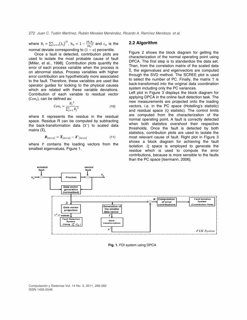
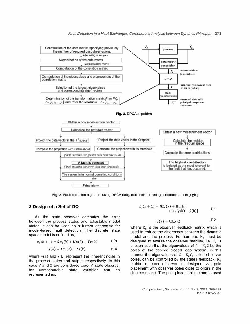
Figure 2 shows the block diagram for getting the characterization of the normal operating point using DPCA. The first step is to standardize the data set. Then, from the correlation matrix of the scaled data X, the eigenvalues and eigenvectors are computed through the SVD method. The SCREE plot is used to select the number of PC. Finally, the matrix T is back-transformed into the original data coordination system including only the PC variances. Left plot in Figure 3 displays the block diagram for applying DPCA in the online fault detection task. The new measurements are projected onto the loading vectors, i.e. in the PC space (Hotelling’s statistic) and residual space (Q statistic). The control limits are computed from the characterization of the normal operating point. A fault is correctly detected when both statistics overshoot their respective thresholds. Once the fault is detected by both statistics, contribution plots are used to isolate the most relevant cause of fault. Right plot in Figure 3 shows a block diagram for achieving the fault isolation .Q space is employed to generate the residue which is used to compute the error contributions, because is more sensible to the faults than the PC space [Isermann, 2006].

Fig. 1. FDI system using DPCA



Fig. 2. DPCA algorithm

Fig. 3. Fault detection algorithm using DPCA (left), fault isolation using contribution plots (right)

3 Design of a Set of DO

As the state observer computes the error between the process states and adjustable model states, it can be used as a further alternative for model-based fault detection. The discrete state space model is defined as,

1 (12)

(13)

where v k and z k represent the inherent noise in the process states and output, respectively. In this case V and Z are considered zero. A state observer for unmeasurable state variables can be represented as,

x k 1 Gx k Hu k

K y k y k (14)

y k Cx k (15)

where K is the observer feedback matrix, which is used to reduce the differences between the dynamic model and the process. Furthermore, K must be designed to ensure the observer stability, i.e. K is chosen such that the eigenvalues of G K C be the poles of the desired closed loop system, in this manner the eigenvalues of G K C, called observer poles, can be controlled by the states feedback. K matrix in each observer is designed via pole placement with observer poles close to origin in the discrete space. The pole placement method is used



to find K which guarantees the convergence speed and observer stability. 3.1 FDD using a Set of DO The error of the observer can be computed as,

x k 1 x k 1 G K C x x (16)

Defining e k x k x k as the error vector, the predicted error can be calculated as,

e k 1 G K C e k (17)

The dynamic behavior of the error signal e k is determined by the eigenvalues of G K C. If the matrix G K C is a stable matrix, the error vector will converge to zero for any initial error e 0 . In order to ensure the stability of the matrix G K C, the observer feedback matrix K must be computed properly to achieve pole placement. The design of a set of DO can be reviewed in detail in [Tudón, 2008].

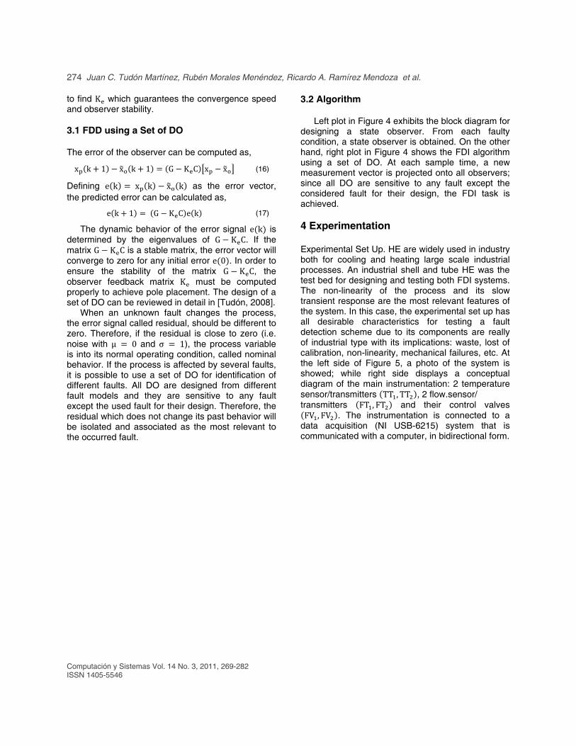
When an unknown fault changes the process, the error signal called residual, should be different to zero. Therefore, if the residual is close to zero (i.e. noise with µ 0 and σ 1), the process variable is into its normal operating condition, called nominal behavior. If the process is affected by several faults, it is possible to use a set of DO for identification of different faults. All DO are designed from different fault models and they are sensitive to any fault except the used fault for their design. Therefore, the residual which does not change its past behavior will be isolated and associated as the most relevant to the occurred fault.

3.2 Algorithm

Left plot in Figure 4 exhibits the block diagram for designing a state observer. From each faulty condition, a state observer is obtained. On the other hand, right plot in Figure 4 shows the FDI algorithm using a set of DO. At each sample time, a new measurement vector is projected onto all observers; since all DO are sensitive to any fault except the considered fault for their design, the FDI task is achieved.

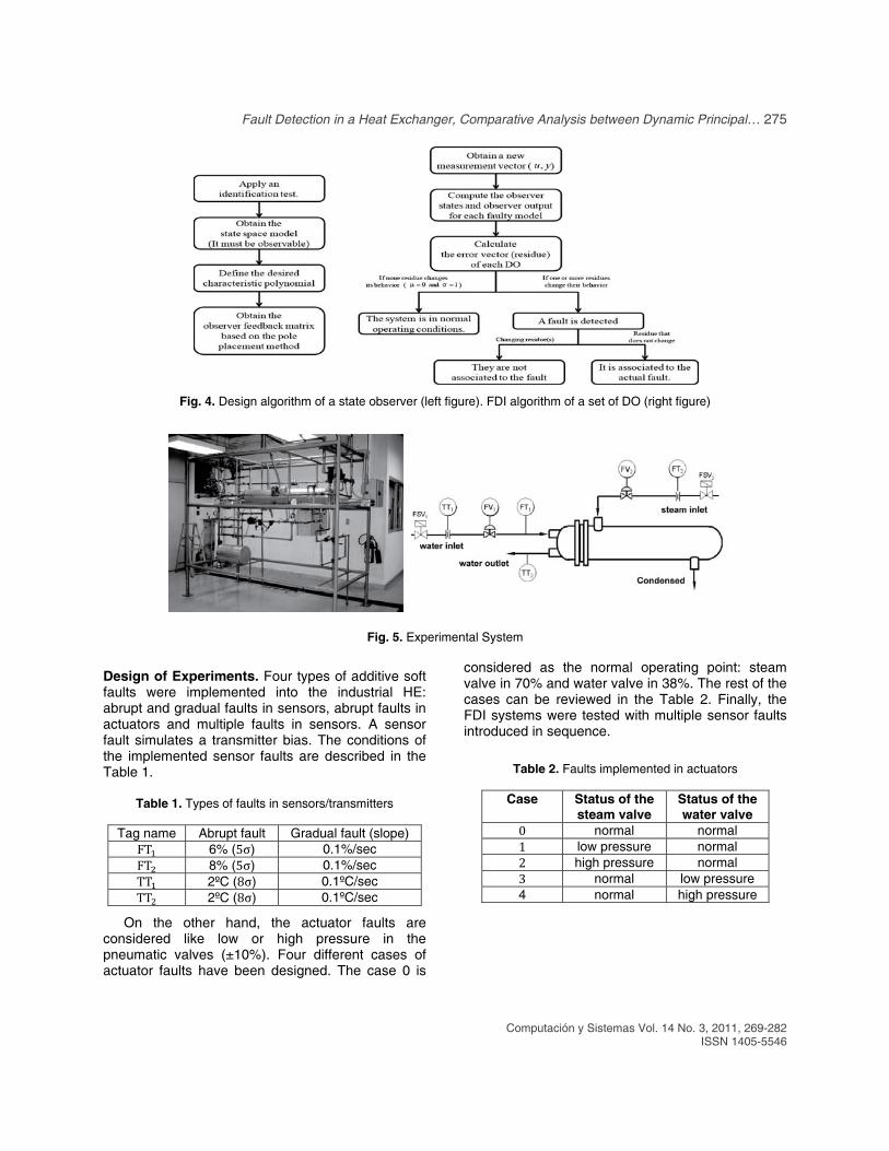
4 Experimentation Experimental Set Up. HE are widely used in industry both for cooling and heating large scale industrial processes. An industrial shell and tube HE was the test bed for designing and testing both FDI systems. The non-linearity of the process and its slow transient response are the most relevant features of the system. In this case, the experimental set up has all desirable characteristics for testing a fault detection scheme due to its components are really of industrial type with its implications: waste, lost of calibration, non-linearity, mechanical failures, etc. At the left side of Figure 5, a photo of the system is showed; while right side displays a conceptual diagram of the main instrumentation: 2 temperature sensor/transmitters. TT , TT ,.2.flow.sensor/ transmitters FT , FT and their control valves FV , FV . The instrumentation is connected to a

data acquisition (NI USB-6215) system that is communicated with a computer, in bidirectional form.



Fig. 4. Design algorithm of a state observer (left figure). FDI algorithm of a set of DO (right figure)

Fig. 5. Experimental System

Design of Experiments. Four types of additive soft faults were implemented into the industrial HE: abrupt and gradual faults in sensors, abrupt faults in actuators and multiple faults in sensors. A sensor fault simulates a transmitter bias. The conditions of the implemented sensor faults are described in the Table 1.

Table 1. Types of faults in sensors/transmitters

Tag name Abrupt fault Gradual fault (slope) FT 6% (5σ) 0.1%/sec FT 8% (5σ) 0.1%/sec TT 2ºC (8σ) 0.1ºC/sec TT 2ºC (8σ) 0.1ºC/sec

On the other hand, the actuator faults are considered like low or high pressure in the pneumatic valves (±10%). Four different cases of actuator faults have been designed. The case 0 is

considered as the normal operating point: steam valve in 70% and water valve in 38%. The rest of the cases can be reviewed in the Table 2. Finally, the FDI systems were tested with multiple sensor faults introduced in sequence.

Table 2. Faults implemented in actuators

Case Status of the

steam valve Status of the water valve

0 normal normal 1 low pressure normal 2 high pressure normal 3 normal low pressure 4 normal high pressure



For comparison, same metrics have been monitored in both approaches: quick detection, isolability capacity, explanation facility, false alarm rates, robustness for detecting different faults and multiple faults identifiability.

5 Results for DPCA

Training Stage. DPCA uses 1 second of sample time for this step; and 1900 measurement data of each sensor were taken. Thus, the data vector is defined by,

(18)

By taking 1 past observation of each measurement, it is possible to explain a high quantity of variance including the possible auto and cross correlations. Table 3 shows the characterization of the normal operating point using DPCA; with 5 PC, it can be explained the 99.94% of total variance and 1 more PC does not improve the quality of data representation.

Table 3. Process characterization

PC Eigenvalue Explained

variance (%) Cumulative Explained

Variance (%) 1 3.1361 39.20 39.20 2 2.0643 25.80 65.00 3 1.3861 17.32 82.33 4 0.9925 12.40 94.73 5 0.4167 5.20 99.94 6 0.0013 0.01 99.96 7 0.0003 0.00 99.96 8 0.0002 0.00 99.96

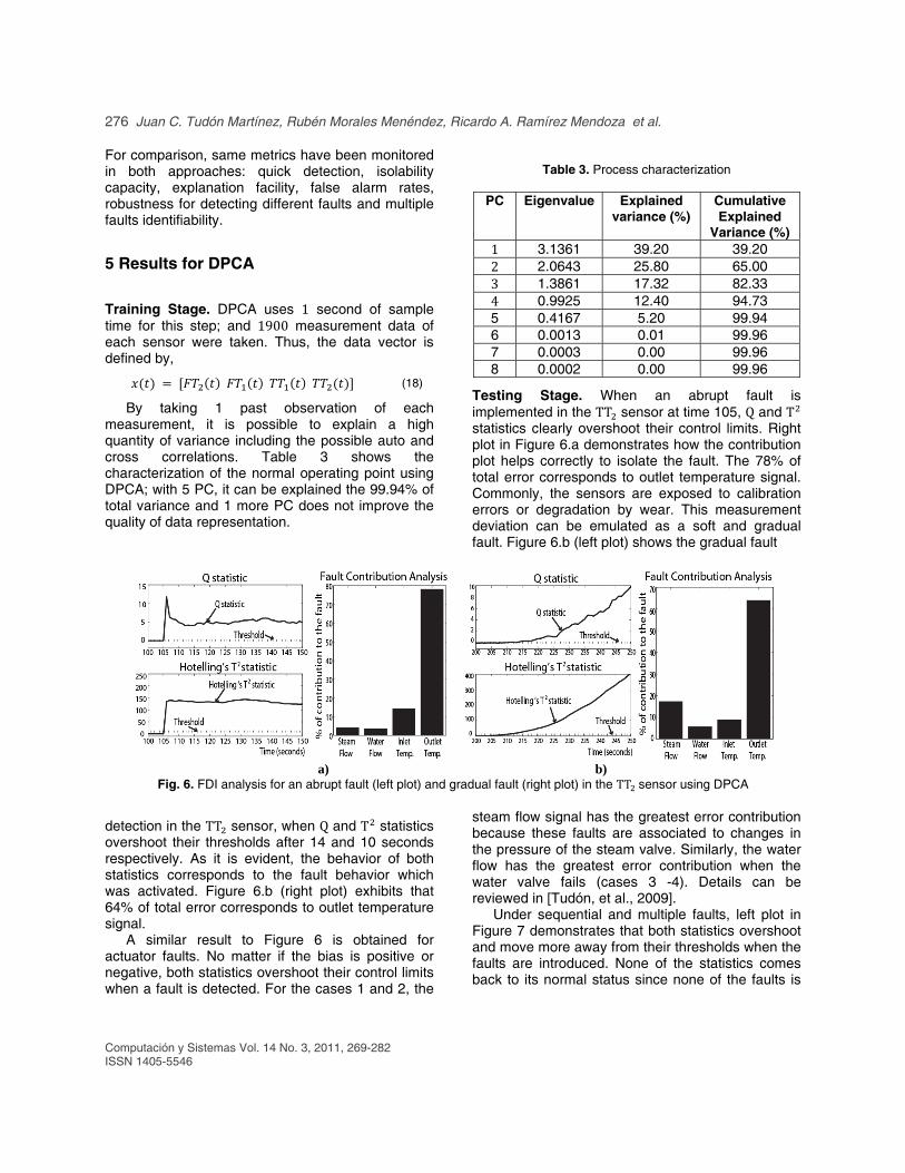
Testing Stage. When an abrupt fault is implemented in the TT sensor at time 105, Q and T statistics clearly overshoot their control limits. Right plot in Figure 6.a demonstrates how the contribution plot helps correctly to isolate the fault. The 78% of total error corresponds to outlet temperature signal. Commonly, the sensors are exposed to calibration errors or degradation by wear. This measurement deviation can be emulated as a soft and gradual fault. Figure 6.b (left plot) shows the gradual fault

a) b)

Fig. 6. FDI analysis for an abrupt fault (left plot) and gradual fault (right plot) in the TT sensor using DPCA

detection in the TT sensor, when Q and T statistics overshoot their thresholds after 14 and 10 seconds respectively. As it is evident, the behavior of both statistics corresponds to the fault behavior which was activated. Figure 6.b (right plot) exhibits that 64% of total error corresponds to outlet temperature signal.

A similar result to Figure 6 is obtained for actuator faults. No matter if the bias is positive or negative, both statistics overshoot their control limits when a fault is detected. For the cases 1 and 2, the

steam flow signal has the greatest error contribution because these faults are associated to changes in the pressure of the steam valve. Similarly, the water flow has the greatest error contribution when the water valve fails (cases 3 -4). Details can be reviewed in [Tudón, et al., 2009].

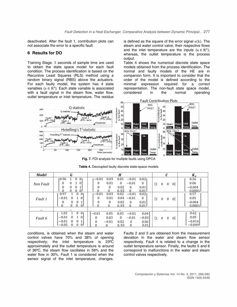
Under sequential and multiple faults, left plot in Figure 7 demonstrates that both statistics overshoot and move more away from their thresholds when the faults are introduced. None of the statistics comes back to its normal status since none of the faults is



deactivated. After the fault 1, contribution plots can not associate the error to a specific fault.

6 Results for DO Training Stage. 5 seconds of sample time are used to obtain the state space model for each fault condition. The process identification is based on the Recursive Least Squares (RLS) method using a random binary signal (RBS) above the actuators. For each faulty model, the system has 4 state variables (x ). Each state variable is associated with a fault signal in the steam flow, water flow, outlet temperature or inlet temperature. The residue

is defined as the square of the error signal e k . The steam and water control valve, their respective flows and the inlet temperature are the inputs (u ); whereas, the outlet temperature is the process output. Table 4 shows the numerical discrete state space models obtained from the process identification. The normal and faulty models of the HE are in companion form. It is important to consider that the order of the model is defined according to the minimal expression required for a correct representation. The non-fault state space model, considered in the normal operating

Fig. 7. FDI analysis for multiple faults using DPCA

Table 4. Decoupled faulty discrete state-space models

Model

Non Fault

0.96 1 00 0 10 0 0

0 0 0

001

0

0.01 0.03 0.010 0.01 00 0 0.02

0 0 0. 03

0.01 0.020.01 00 0.010 0.01

1 0 0 0

0.560.060.004

0.0001

Fault 1

0.97 1 00.01 0 10 0 0

0 0 0

001

0

0.01 0.03 0.020 0.01 0.040 0 0.02

0 0 0. 03

0.01 0.020.01 00 0.010 0.01

1 0 0 0

0.570.050.004

0.0001

… … … … …

Fault 6 1.02 1 0

0.01 0 10.01 0 00.05 0 0

001

0

0.01 0.05 0.03 0 0.03 0 0 0.01 0.02

0 0 0. 03

0.01 0.040.01 0.030 0.060 0.01

1 0 0 0

0.62 0.05

0.014 0.049

conditions, is obtained when the steam and water control valves have 70% and 38% of opening respectively; the inlet temperature is 23ºC approximately and the outlet temperature is around of 36ºC, the steam flow oscillates in 58% and the water flow in 30%. Fault 1 is considered when the sensor signal of the inlet temperature, changes.

Faults 2 and 3 are obtained from the measurement deviation in the water and steam flow sensor respectively. Fault 4 is related to a change in the outlet temperature sensor. Finally, the faults 5 and 6 correspond to malfunctions in the water and steam control valves respectively.



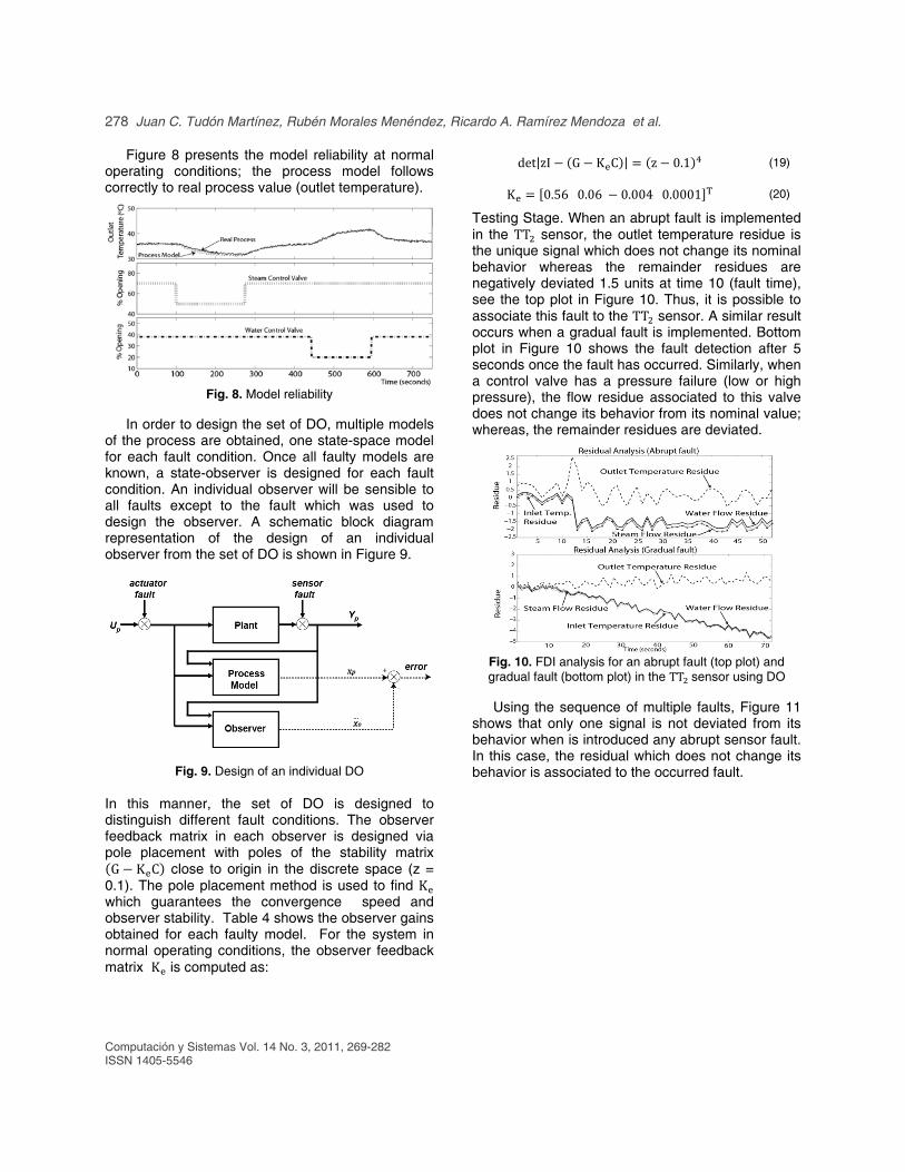
Figure 8 presents the model reliability at normal operating conditions; the process model follows correctly to real process value (outlet temperature).

Fig. 8. Model reliability

In order to design the set of DO, multiple models

of the process are obtained, one state-space model for each fault condition. Once all faulty models are known, a state-observer is designed for each fault condition. An individual observer will be sensible to all faults except to the fault which was used to design the observer. A schematic block diagram representation of the design of an individual observer from the set of DO is shown in Figure 9.

Fig. 9. Design of an individual DO

In this manner, the set of DO is designed to distinguish different fault conditions. The observer feedback matrix in each observer is designed via pole placement with poles of the stability matrix G K C close to origin in the discrete space (z =

0.1). The pole placement method is used to find K which guarantees the convergence speed and observer stability. Table 4 shows the observer gains obtained for each faulty model. For the system in normal operating conditions, the observer feedback matrix K is computed as:

det|zI G K C | z 0.1 (19)

K 0.56 0.06 0.004 0.0001 T (20)

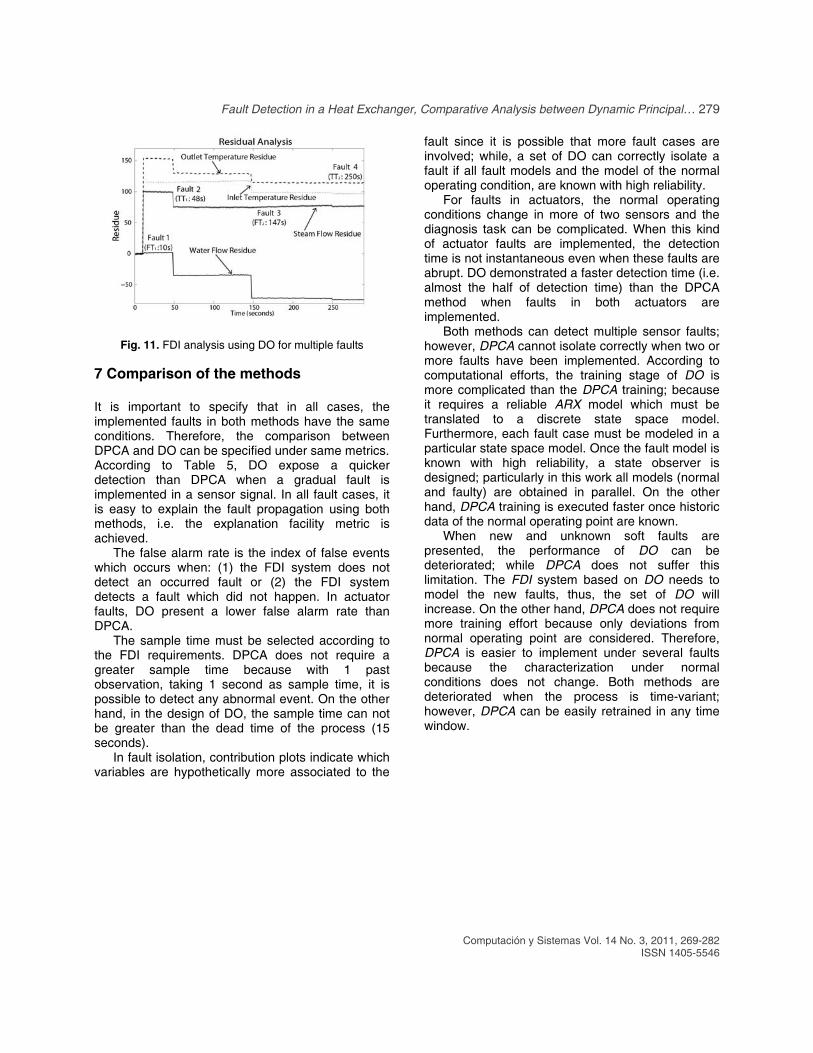
Testing Stage. When an abrupt fault is implemented in the TT sensor, the outlet temperature residue is the unique signal which does not change its nominal behavior whereas the remainder residues are negatively deviated 1.5 units at time 10 (fault time), see the top plot in Figure 10. Thus, it is possible to associate this fault to the TT sensor. A similar result occurs when a gradual fault is implemented. Bottom plot in Figure 10 shows the fault detection after 5 seconds once the fault has occurred. Similarly, when a control valve has a pressure failure (low or high pressure), the flow residue associated to this valve does not change its behavior from its nominal value; whereas, the remainder residues are deviated.

Fig. 10. FDI analysis for an abrupt fault (top plot) and gradual fault (bottom plot) in the TT sensor using DO

Using the sequence of multiple faults, Figure 11

shows that only one signal is not deviated from its behavior when is introduced any abrupt sensor fault. In this case, the residual which does not change its behavior is associated to the occurred fault.



Fig. 11. FDI analysis using DO for multiple faults

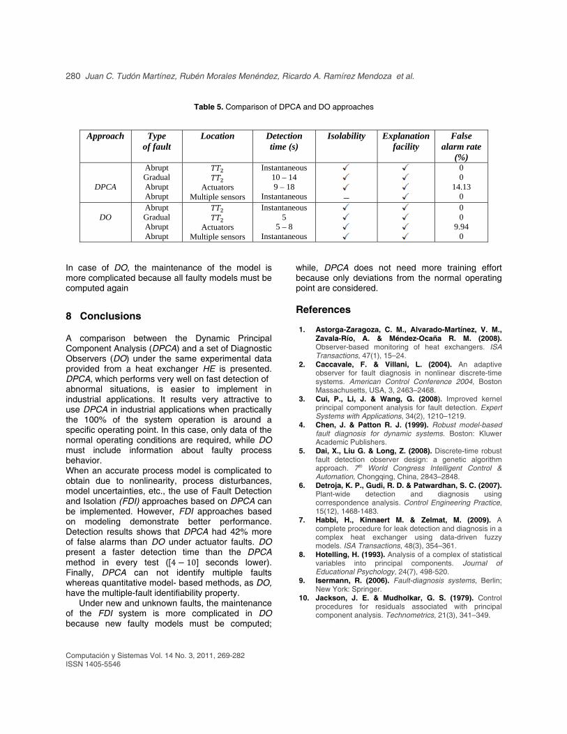
7 Comparison of the methods It is important to specify that in all cases, the implemented faults in both methods have the same conditions. Therefore, the comparison between DPCA and DO can be specified under same metrics. According to Table 5, DO expose a quicker detection than DPCA when a gradual fault is implemented in a sensor signal. In all fault cases, it is easy to explain the fault propagation using both methods, i.e. the explanation facility metric is achieved.

The false alarm rate is the index of false events which occurs when: (1) the FDI system does not detect an occurred fault or (2) the FDI system detects a fault which did not happen. In actuator faults, DO present a lower false alarm rate than DPCA.

The sample time must be selected according to the FDI requirements. DPCA does not require a greater sample time because with 1 past observation, taking 1 second as sample time, it is possible to detect any abnormal event. On the other hand, in the design of DO, the sample time can not be greater than the dead time of the process (15 seconds).

In fault isolation, contribution plots indicate which variables are hypothetically more associated to the

fault since it is possible that more fault cases are involved; while, a set of DO can correctly isolate a fault if all fault models and the model of the normal operating condition, are known with high reliability.

For faults in actuators, the normal operating conditions change in more of two sensors and the diagnosis task can be complicated. When this kind of actuator faults are implemented, the detection time is not instantaneous even when these faults are abrupt. DO demonstrated a faster detection time (i.e. almost the half of detection time) than the DPCA method when faults in both actuators are implemented.

Both methods can detect multiple sensor faults; however, DPCA cannot isolate correctly when two or more faults have been implemented. According to computational efforts, the training stage of DO is more complicated than the DPCA training; because it requires a reliable ARX model which must be translated to a discrete state space model. Furthermore, each fault case must be modeled in a particular state space model. Once the fault model is known with high reliability, a state observer is designed; particularly in this work all models (normal and faulty) are obtained in parallel. On the other hand, DPCA training is executed faster once historic data of the normal operating point are known.

When new and unknown soft faults are presented, the performance of DO can be deteriorated; while DPCA does not suffer this limitation. The FDI system based on DO needs to model the new faults, thus, the set of DO will increase. On the other hand, DPCA does not require more training effort because only deviations from normal operating point are considered. Therefore, DPCA is easier to implement under several faults because the characterization under normal conditions does not change. Both methods are deteriorated when the process is time-variant; however, DPCA can be easily retrained in any time window.



Table 5. Comparison of DPCA and DO approaches

In case of DO, the maintenance of the model is more complicated because all faulty models must be computed again

8 Conclusions

A comparison between the Dynamic Principal Component Analysis (DPCA) and a set of Diagnostic Observers (DO) under the same experimental data provided from a heat exchanger HE is presented. DPCA, which performs very well on fast detection of abnormal situations, is easier to implement in industrial applications. It results very attractive to use DPCA in industrial applications when practically the 100% of the system operation is around a specific operating point. In this case, only data of the normal operating conditions are required, while DO must include information about faulty process behavior. When an accurate process model is complicated to obtain due to nonlinearity, process disturbances, model uncertainties, etc., the use of Fault Detection and Isolation (FDI) approaches based on DPCA can be implemented. However, FDI approaches based on modeling demonstrate better performance. Detection results shows that DPCA had 42% more of false alarms than DO under actuator faults. DO present a faster detection time than the DPCA method in every test ([4 10] seconds lower). Finally, DPCA can not identify multiple faults whereas quantitative model- based methods, as DO, have the multiple-fault identifiability property.

Under new and unknown faults, the maintenance of the FDI system is more complicated in DO because new faulty models must be computed;

while, DPCA does not need more training effort because only deviations from the normal operating point are considered.

References

1. Astorga-Zaragoza, C. M., Alvarado-Martínez, V. M.,

Zavala-Río, A. & Méndez-Ocaña R. M. (2008). Observer-based monitoring of heat exchangers. ISA Transactions, 47(1), 15–24.

2. Caccavale, F. & Villani, L. (2004). An adaptive observer for fault diagnosis in nonlinear discrete-time systems. American Control Conference 2004, Boston Massachusetts, USA, 3, 2463–2468.

3. Cui, P., Li, J. & Wang, G. (2008). Improved kernel principal component analysis for fault detection. Expert Systems with Applications, 34(2), 1210–1219.

4. Chen, J. & Patton R. J. (1999). Robust model-based fault diagnosis for dynamic systems. Boston: Kluwer Academic Publishers.

5. Dai, X., Liu G. & Long, Z. (2008). Discrete-time robust fault detection observer design: a genetic algorithm approach. 7th World Congress Intelligent Control & Automation, Chongqing, China, 2843–2848.

6. Detroja, K. P., Gudi, R. D. & Patwardhan, S. C. (2007). Plant-wide detection and diagnosis using correspondence analysis. Control Engineering Practice, 15(12), 1468-1483.

7. Habbi, H., Kinnaert M. & Zelmat, M. (2009). A complete procedure for leak detection and diagnosis in a complex heat exchanger using data-driven fuzzy models. ISA Transactions, 48(3), 354–361.

8. Hotelling, H. (1993). Analysis of a complex of statistical variables into principal components. Journal of Educational Psychology, 24(7), 498-520.

9. Isermann, R. (2006). Fault-diagnosis systems, Berlin; New York: Springer.

10. Jackson, J. E. & Mudholkar, G. S. (1979). Control procedures for residuals associated with principal component analysis. Technometrics, 21(3), 341–349.

Approach Type of fault

Location Detection time (s)

Isolability Explanation facility

False alarm rate

(%)

DPCA

Abrupt Gradual Abrupt Abrupt

Actuators Multiple sensors

Instantaneous 10 – 14 9 – 18

Instantaneous

―

0 0

14.13 0

DO

Abrupt Gradual Abrupt Abrupt

Actuators Multiple sensors

Instantaneous 5

5 – 8 Instantaneous

0 0

9.94 0



11. Krishnan, R. A. & Pappa, N. (2005). Real time fault diagnosis for a heat exchanger - a model based approach. 2005 Annual IEEE INDICON, Chennai, India, 78–82.

12. Ku, W., Storer, R. H. & Georgakis, C. (1995). Disturbance detection and isolation by dynamic principal component analysis. Chemometrics and Intelligent Laboratory Systems, 30(1), 179–196.

13. Lingfang, S., Yingying, Z. & Rina, S. (2009). Research on the fouling prediction of heat exchanger based on Support Vector Machine optimized by particle swarm optimization algorithm. International Conference on Mechatronics and Automation, Changchun, China, 2002–2007.

14. Miller, P., Swanson, R. E. & Heckler, C. E. (1998). Contribution plots: a missing link in multivariate quality control. International Journal of Applied Mathematics and Computer Science, 8(4), pp: 775–792.

15. Mina, J. & Verde, C. (2007). Fault detection for MIMO systems integrating multivariate statistical analysis and identification methods. American Control Conference 2007, New York, USA, 3234–3239.

16. Morales-Menendez, R., de Freitas, N., & Poole, D. (2003). Estimation and control of industrial processes with particle filters. American Control Conference 2003, Denver Colorado, USA, 579–584.

17. Parera, A., Papamichail, N., Barsan, N., Weimar, U. & Marco, S. (2006). On-line novelty detection by recursive dynamic principal component analysis and gas sensor arrays under drift conditions. IEEE Sensors Journal, 6(3), 770–783.

18. Puig, V., Quevedo, J., Escobet T., Nejjari F. & de las Heras, S. (2008). Passive robust fault detection of dynamic processes using interval models. IEEE Transactions on Control Systems Technology, 16(5), 1083–1089.

19. Rea-Palacios, C., Morales-Menendez, R. & Verde-Rodarte, C. (2008). Identificación de fallas en un intercambiador de calor. Research in Computing Science, México D.F., 36, 3–12.

20. Simmani, S. & Patton, R. J. (2008). Fault diagnosis of an industrial gas turbine prototype using a system identification approach. Control Engineering Practice, 16(7), 769–786.

21. Tudón-Martínez, J.C. (2008). Fault detection and diagnosis in a heat exchanger using DPCA and diagnostic observers. MSc thesis, Tecnológico de Monterrey, Monterrey Nuevo León, México.

22. Tudón-Martínez, J. C., Morales-Menendez, R., & Garza-Castañón, L. E. (2009). Fault detection and diagnosis in a heat exchanger. 6th International Conference on Informatics in Control, Automation and Robotics ICINCO 2009, Milan, Italy, 265-270.

23. Venkatasubramanian, V., Rengaswamy, R., Kavuri, S., & Yin, K. (2003). A review of process fault detection and diagnosis part I quantitative model-based methods. Computers & Chemical Engineering, 27(3), 293–311.

24. Verde, C. (2001). Multi-leak detection and isolation in fluid pipelines. Control Engineering Practice, 9(6), 673–682.

25. Wu, D. & Ho, W. C. (2009). Fuzzy filter design for itô stochastic systems with application to sensor fault detection. IEEE Transactions on Fuzzy Systems, 17(1), 233–242.

Juan Carlos Tudón Martínez

Obtained the degree of B.Sc. in Chemical Engineering with honors on May 2006 and the M. Sc. degree in Automation on December 2008 from Tecnológico de Monterrey. Actually, he is studying a PhD in Sciences of Engineering. His research is focused in Fault Diagnosis and Fault Tolerant Control.

Rubén Morales Menéndez

Received the B.Sc. in Chemical Engineering and Systems and two M.Sc. degrees in Process Systems and Automation in 1984, 1986 and 1992, respectively. He has a PhD degree in Artificial Intelligence from Tecnológico de Monterrey in 2003. From 2000 to 2003, he was a Visiting Scholar with the Laboratory of Computational Intelligence at University of British Columbia, Canada. He is a consultant specializing in the analysis and design of automatic control systems for continuous processes for more than 22 years. He is member of the National Researchers System of Mexico (level I), and member of IFAC TC 9.3.



Ricardo A. Ramírez Mendoza

Received the B.Sc. in Mechanical and Electrical Engineering and the M.Sc. degrees in Automation in 1988 and 1992, respectively. He has a PhD degree in Automatic Control from Grenoble Institute of Technology in France in 1997. From 1997 to 2004, he was a Associated Professor with the Departament of Mechatronics at Tecnologico de Monterrey Campus Monterrey, Mexico. He is a senior consultant in Vehicle Dynamics and Automotive Control for more than 15 years. He is member of the National Researchers System of Mexico (level I). Currently, he is Dean of Engineering and Architecture at Tecnologico de Monterrey Campus Mexico City.

Luis E. Garza Castañón

Was born on December 15th, 1963, in Monclova, Coahuila. He holds a PhD in Artificial Intelligence from ITESM, Monterrey since 2001, and graduated from the master degree in Control Engineering in 1988, and from Electronic Systems Engineering in 1986. He worked, for about 10 years, in the Control and Automation area in Metallurgical and Metal-mechanic industry. Now, he is a full time professor in the Mechatronics and Automation department at ITESM Monterrey, and is a level 1 member of the Sistema Nacional de Investigadores (SNI). He has published more than 40 articles in Biometrics, Fault Diagnosis and FTC.

Adriana Vargas Martínez

Was born in 1983, and received the B.Sc. in Chemical Engineering with minor in Industrial Systems in 2005 and graduated from a M.Sc. degree in Environmental Systems in 2007. Since 2007 she is a formal student of the PhD in Mechatronics in the Tecnológico de Monterrey. Her research fields include Artificial Intelligence Methods for Fault Tolerant Control.

Documents

Fault Detection in a Heat Exchanger, Comparative … · between Dynamic Principal Component Analysis ... Detección de Fallas en un ... Fault Detection in a Heat Exchanger, Comparative