Embed Size (px)
Citation preview

Fatigue of metallic bridges: the
role of structural health
monitoring in assessment and
life prediction
Marios K Chryssanthopoulos
Growth of UK Transport Systems R
ou
te K
ilo
metr
es
(Bayliss, 2008)
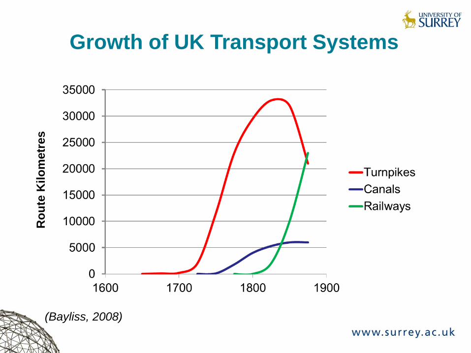
1840 1848
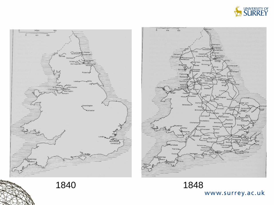
Road
Rail
Pipeline
Water
(DoT/ORR/DECC, 2012)
Domestic goods moved by mode
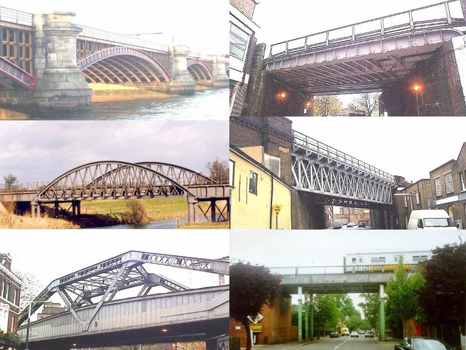
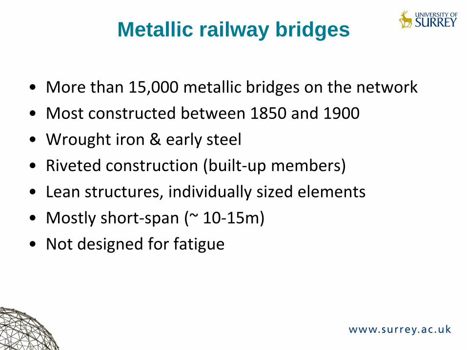
• More than 15,000 metallic bridges on the network
• Most constructed between 1850 and 1900
• Wrought iron & early steel
• Riveted construction (built-up members)
• Lean structures, individually sized elements
• Mostly short-span (~ 10-15m)
• Not designed for fatigue
Metallic railway bridges
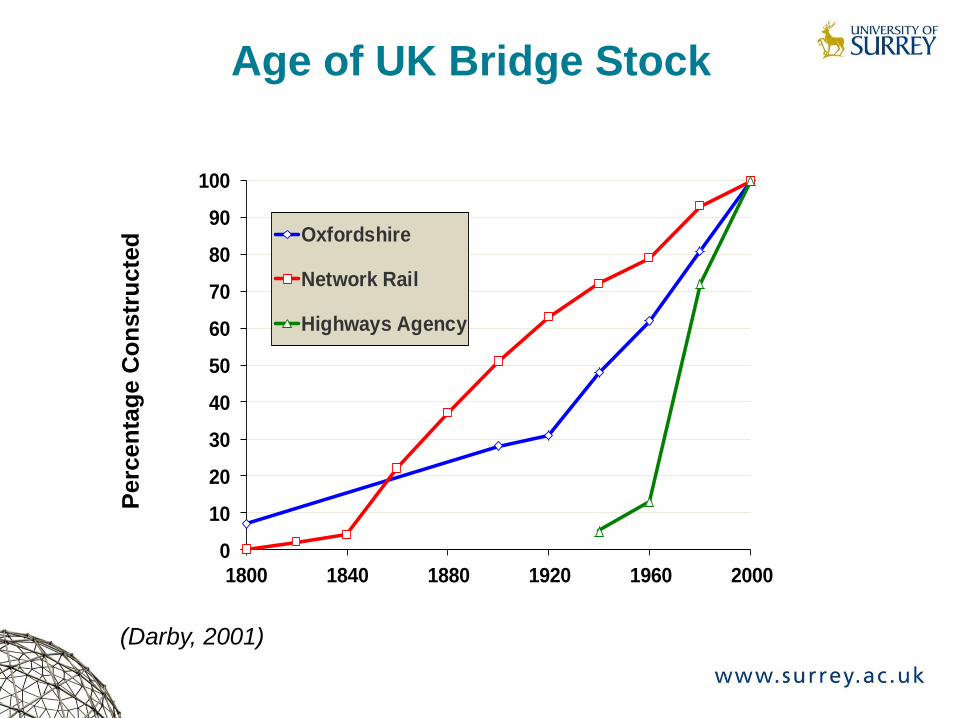
Age of UK Bridge Stock
0
10
20
30
40
50
60
70
80
90
100
1800 1840 1880 1920 1960 2000
Oxfordshire
Network Rail
Highways Agency
(Darby, 2001)
Perc
en
tag
e C
on
str
ucte
d
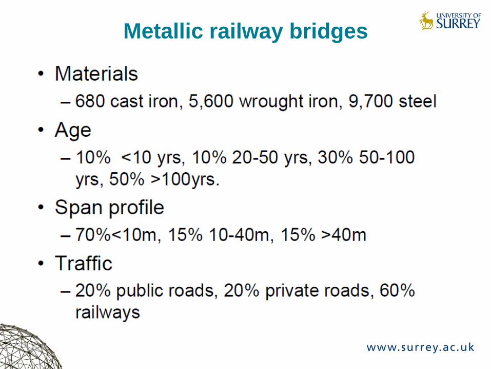
Metallic railway bridges

Wrought iron
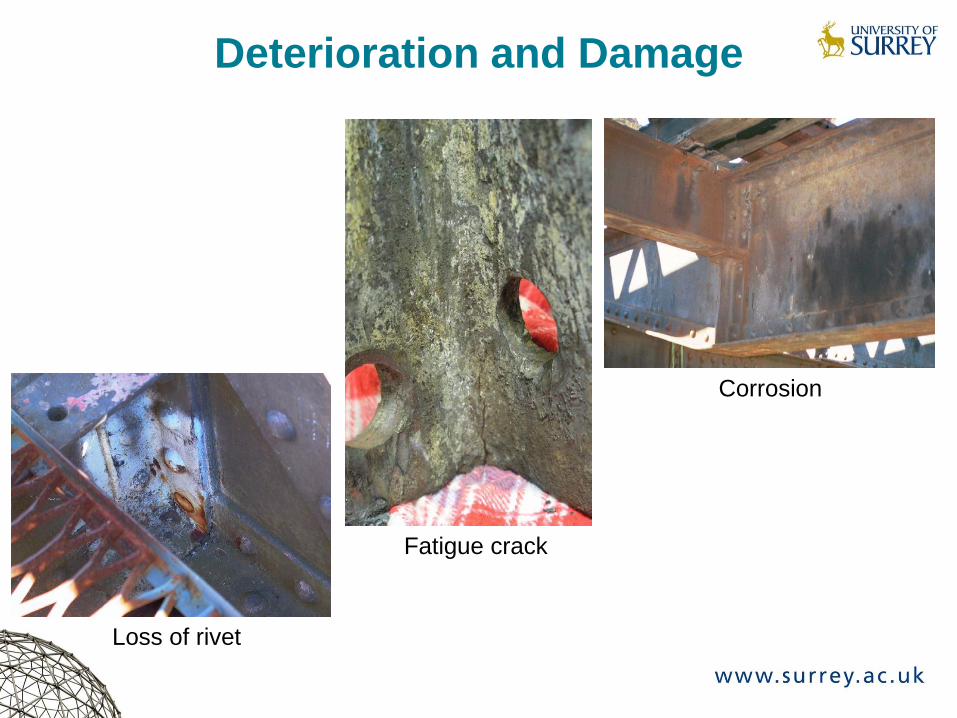
Deterioration and Damage
Corrosion
Fatigue crack
Loss of rivet
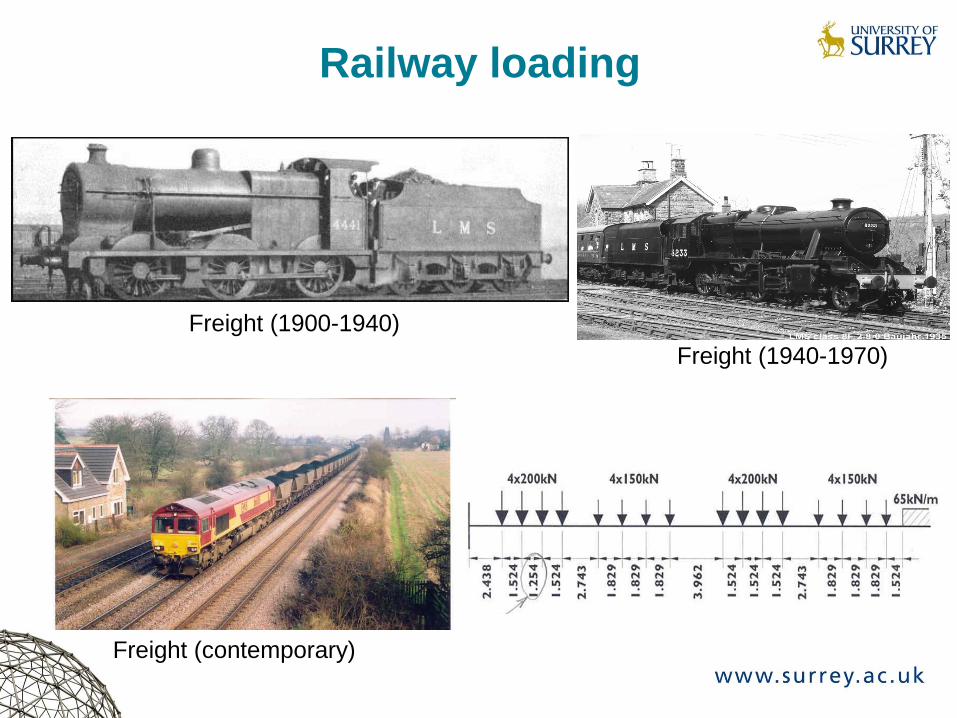
Railway loading
Freight (1900-1940)
Freight (1940-1970)
Freight (contemporary)
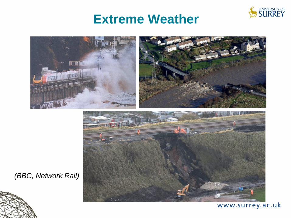
(BBC, Network Rail)
Extreme Weather
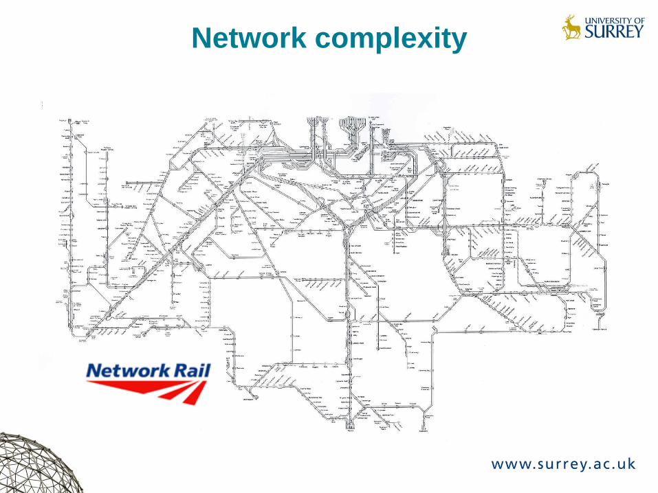
Network complexity
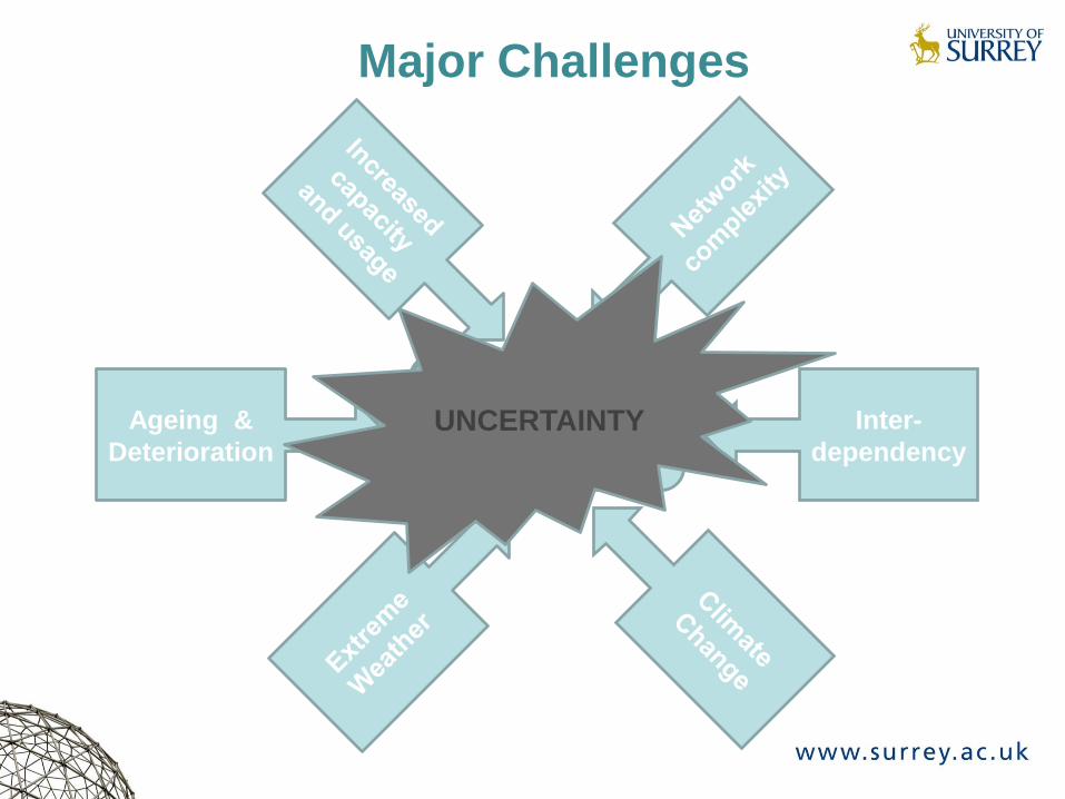
Major Challenges
Ageing &
Deterioration
Inter-
dependency
MAINTENANCE
& RENEWAL
Are assets
safe?
If so, for how
long? At what cost? UNCERTAINTY
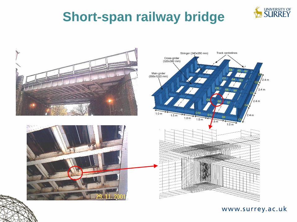
Short-span railway bridge
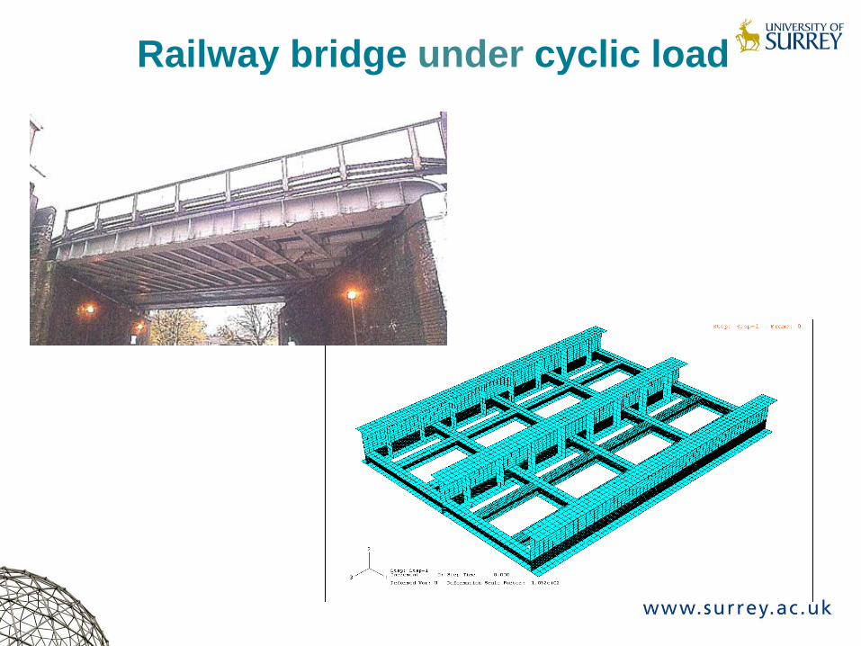
Railway bridge under cyclic load
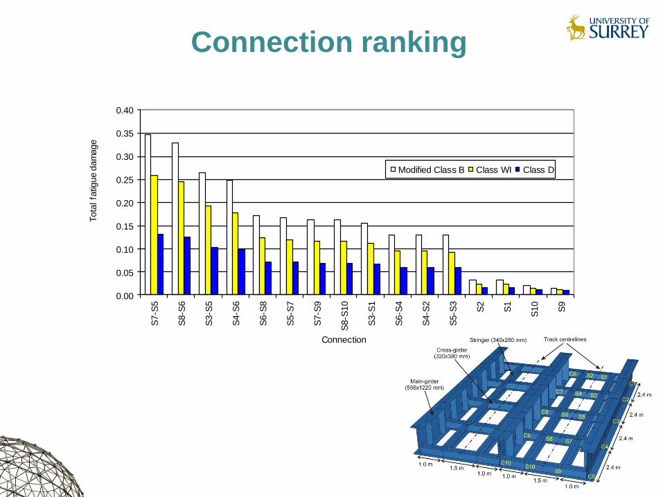
Connection ranking
0.00
0.05
0.10
0.15
0.20
0.25
0.30
0.35
0.40
S7-S
5
S8-S
6
S3-S
5
S4-S
6
S6-S
8
S5-S
7
S7-S
9
S8-S
10
S3-S
1
S6-S
4
S4-S
2
S5-S
3
S2
S1
S10
S9
Tota
l fa
tigue d
am
age
Connection
Modified Class B Class WI Class D
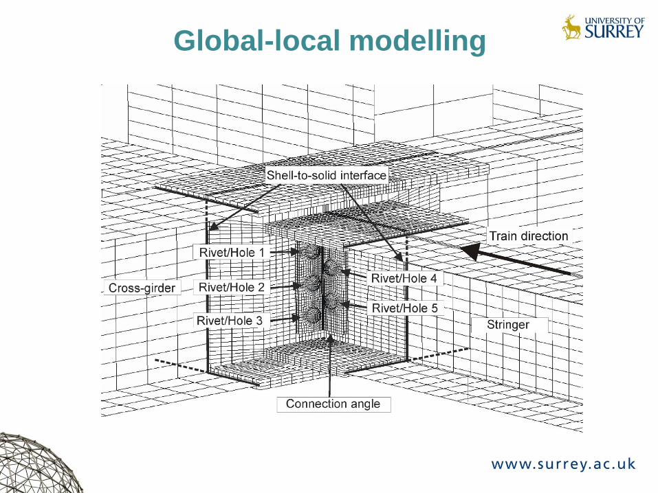
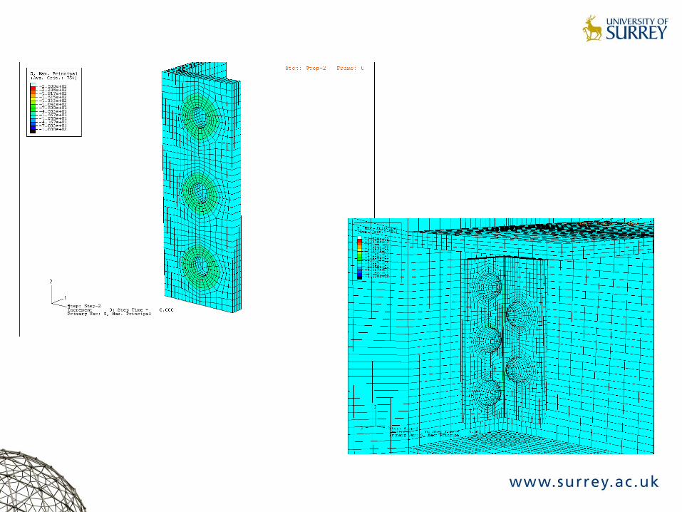
Global-local modelling
0
1
2
3
4
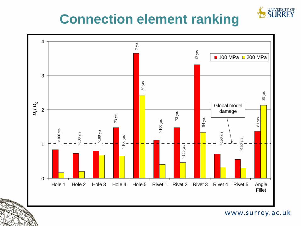
Hole 1 Hole 2 Hole 3 Hole 4 Hole 5 Rivet 1 Rivet 2 Rivet 3 Rivet 4 Rivet 5 AngleFillet
Dl/ D
g
100 MPa 200 MPa
Global model damage
>1
00 y
rs
>1
00
yrs
>10
0 y
rs
>10
0 y
rs
>10
0 y
rs
>1
50
yrs
>1
50
yrs
>1
50
yrs
7 y
rs
12
yrs
81
yrs
30
yrs
84
yrs
39
yrs
73
yrs
73
yrs
Connection element ranking
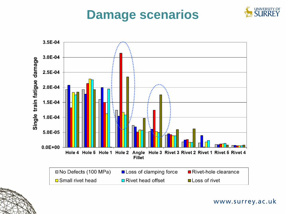
Damage scenarios
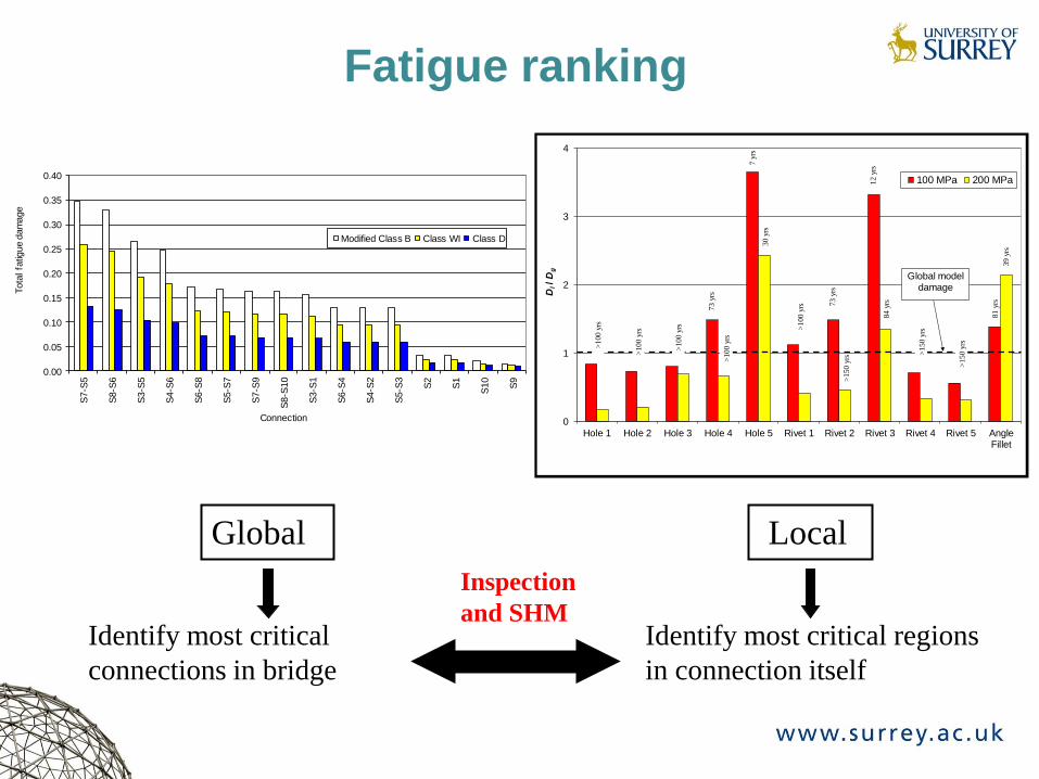
Fatigue ranking
0.00
0.05
0.10
0.15
0.20
0.25
0.30
0.35
0.40
S7-S
5
S8-S
6
S3-S
5
S4-S
6
S6-S
8
S5-S
7
S7-S
9
S8-S
10
S3-S
1
S6-S
4
S4-S
2
S5-S
3
S2
S1
S10
S9
Tota
l fa
tigue d
am
age
Connection
Modified Class B Class WI Class D
Global Local
Identify most critical
connections in bridge
Identify most critical regions
in connection itself
Inspection
and SHM
0
1
2
3
4
Hole 1 Hole 2 Hole 3 Hole 4 Hole 5 Rivet 1 Rivet 2 Rivet 3 Rivet 4 Rivet 5 AngleFillet
Dl/ D
g
100 MPa 200 MPa
Global model damage
>1
00 y
rs
>10
0 y
rs
>10
0 y
rs
>10
0 y
rs
>10
0 y
rs
>15
0 y
rs
>1
50
yrs
>1
50
yrs
7 y
rs
12
yrs
81
yrs
30
yrs
84
yrs
39
yrs
73
yrs
73
yrs
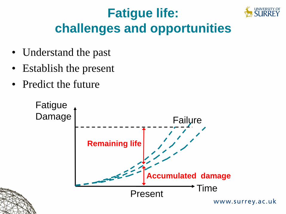
Fatigue life:
challenges and opportunities
• Understand the past
• Establish the present
• Predict the future
Time Present
Accumulated damage
Fatigue
Damage Failure
Remaining life
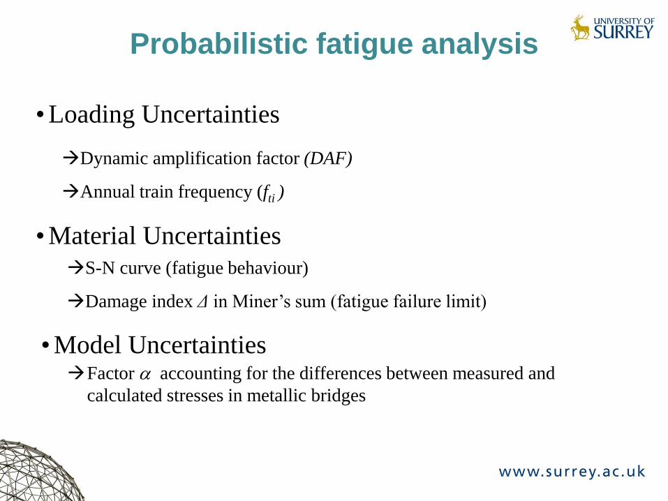
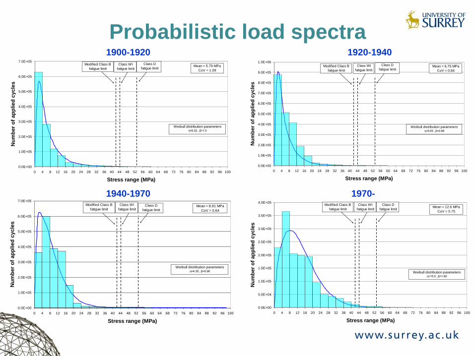
Probabilistic fatigue analysis
• Loading Uncertainties
Dynamic amplification factor (DAF)
Annual train frequency (fti )
• Material Uncertainties
S-N curve (fatigue behaviour)
Damage index Δ in Miner’s sum (fatigue failure limit)
• Model Uncertainties Factor accounting for the differences between measured and
calculated stresses in metallic bridges
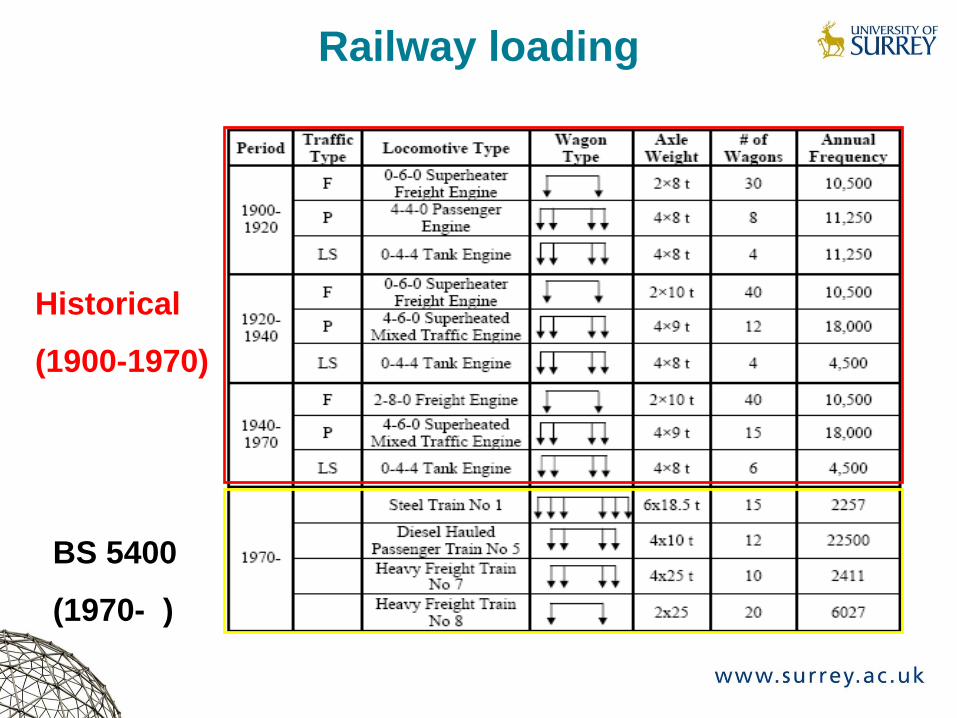
Railway loading
Historical
(1900-1970)
BS 5400
(1970- )
0.0E+00
1.0E+05
2.0E+05
3.0E+05
4.0E+05
5.0E+05
6.0E+05
7.0E+05
0 4 8 12 16 20 24 28 32 36 40 44 48 52 56 60 64 68 72 76 80 84 88 92 96 100
Stress range (MPa)
Nu
mb
er
of
ap
plied
cycle
s
Modified Class B
fatigue limit
Class WI
fatigue limit
Class D
fatigue limitMean = 5.79 MPa
CoV = 1.09
Weibull distribution parametersη=6.02 , β=1.0
0.0E+00
1.0E+05
2.0E+05
3.0E+05
4.0E+05
5.0E+05
6.0E+05
7.0E+05
8.0E+05
9.0E+05
1.0E+06
0 4 8 12 16 20 24 28 32 36 40 44 48 52 56 60 64 68 72 76 80 84 88 92 96 100
Stress range (MPa)
Nu
mb
er
of
ap
plied
cycle
s
Modified Class B
fatigue limit
Class WI
fatigue limit
Class D
fatigue limitMean = 6.75 MPa
CoV = 0.84
Weibull distribution parametersη=5.05 , β=0.98
0.0E+00
1.0E+05
2.0E+05
3.0E+05
4.0E+05
5.0E+05
6.0E+05
7.0E+05
0 4 8 12 16 20 24 28 32 36 40 44 48 52 56 60 64 68 72 76 80 84 88 92 96 100
Stress range (MPa)
Nu
mb
er
of
ap
plied
cycle
s
Modified Class B
fatigue limit
Class WI
fatigue limit Class D
fatigue limitMean = 8.91 MPa
CoV = 0.64
Weibull distribution parametersη=4.35 , β=0.90
0.0E+00
5.0E+04
1.0E+05
1.5E+05
2.0E+05
2.5E+05
3.0E+05
3.5E+05
4.0E+05
0 4 8 12 16 20 24 28 32 36 40 44 48 52 56 60 64 68 72 76 80 84 88 92 96 100
Stress range (MPa)
Nu
mb
er
of
ap
plied
cycle
s
Modified Class B
fatigue limit
Class WI
fatigue limit
Class D
fatigue limitMean = 12.6 MPa
CoV = 0.75
Weibull distribution parametersη=15.0 , β=1.60
1900-1920
Probabilistic load spectra 1920-1940
1940-1970 1970-
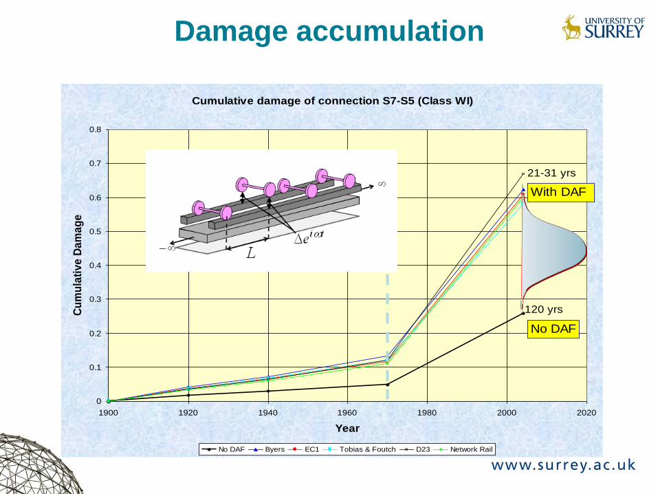
Cumulative damage of connection S7-S5 (Class WI)
0
0.1
0.2
0.3
0.4
0.5
0.6
0.7
0.8
1900 1920 1940 1960 1980 2000 2020
Year
Cu
mu
lati
ve
Da
ma
ge
No DAF Byers EC1 Tobias & Foutch D23 Network Rail
21-31 yrs
120 yrs
No DAF
With DAF
Damage accumulation
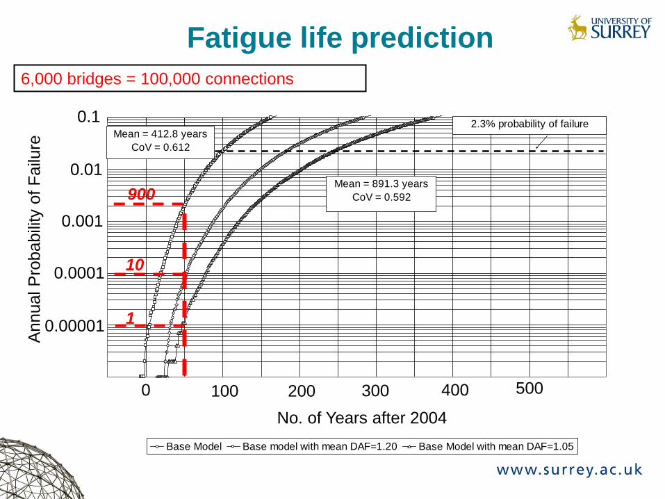
0.000001
0.00001
0.0001
0.001
0.01
0.1
-50 0 50 100 150 200 250 300 350 400 450 500 550 600
Time after 2004 (years)
Pro
ba
bil
ity
of
fail
ure
Pf
Base Model Base model with mean DAF=1.20 Base Model with mean DAF=1.05
2.3% probability of failureMean = 412.8 years
CoV = 0.612
Mean = 891.3 years
CoV = 0.592
200 100 0
0.1
0.01
0.0001
300
0.001
0.00001
Fatigue life prediction
No. of Years after 2004
Annual P
robabili
ty o
f F
ailu
re
400 500
6,000 bridges = 100,000 connections
900
10
1
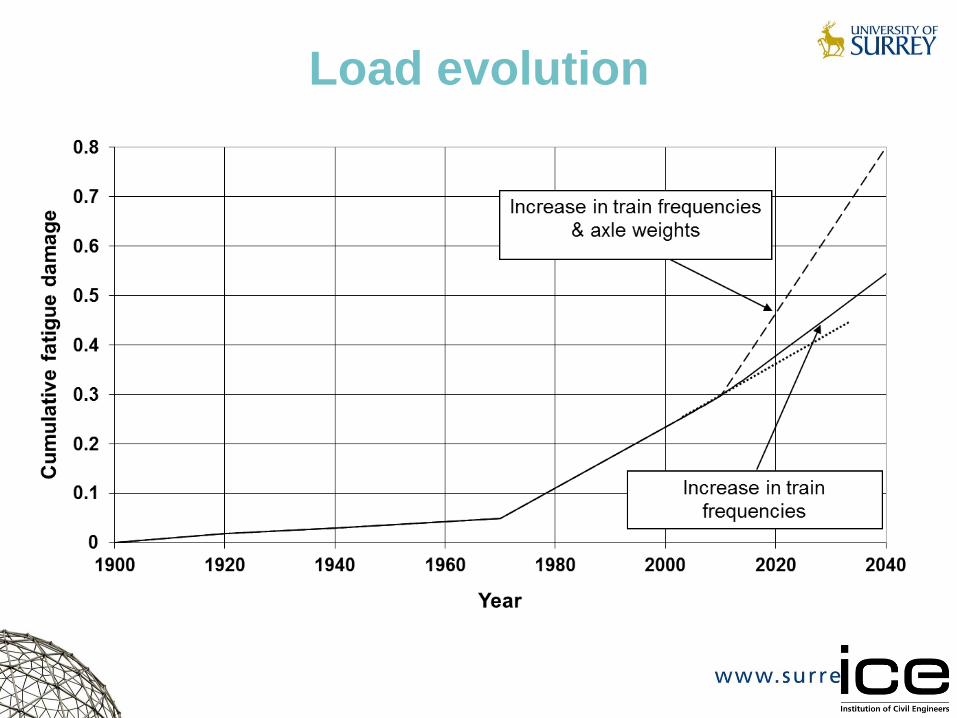
Load evolution
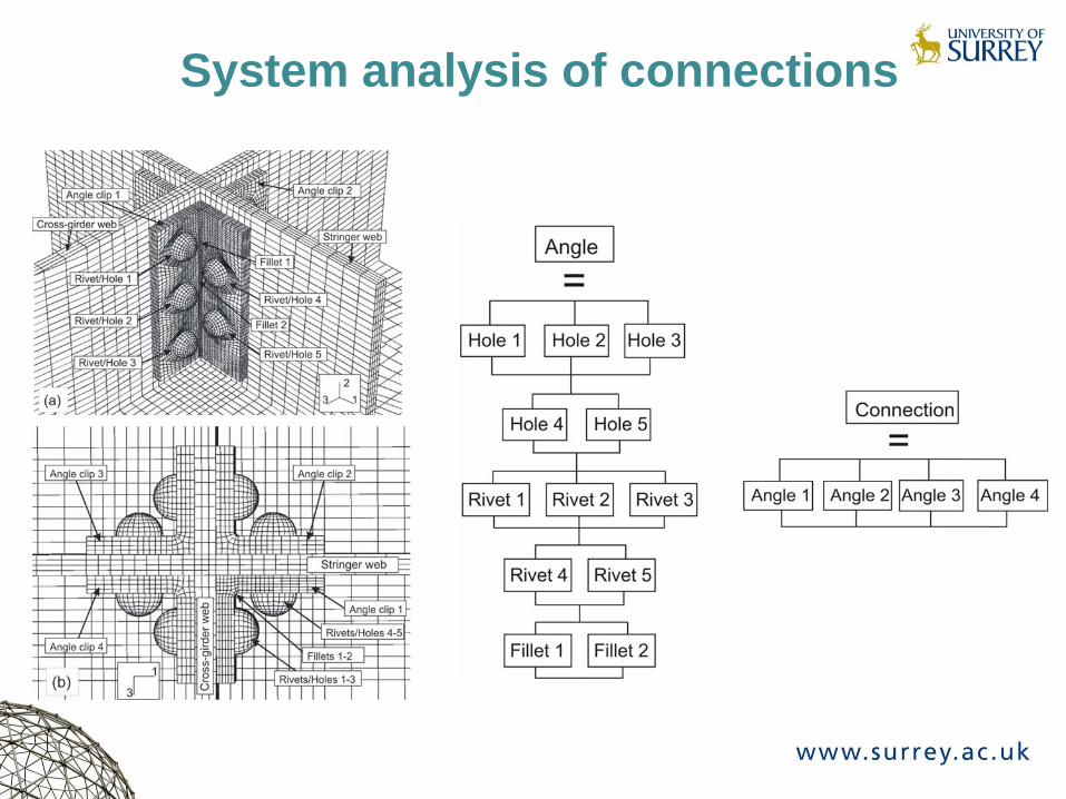
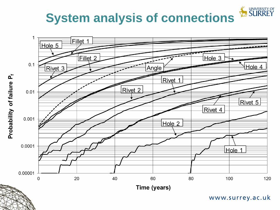
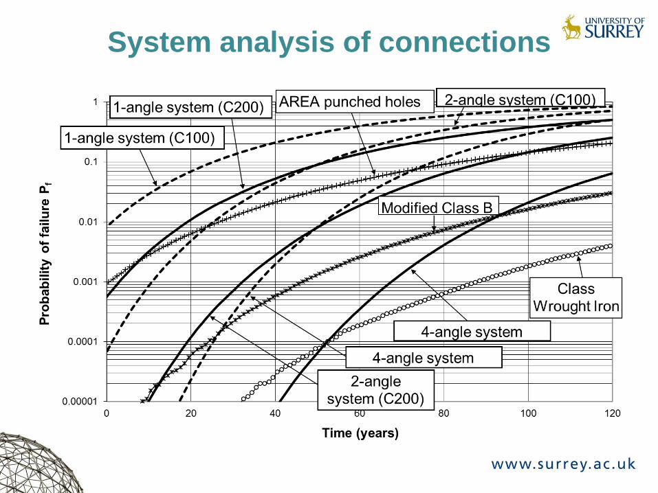
System analysis of connections
System analysis of connections
System analysis of connections
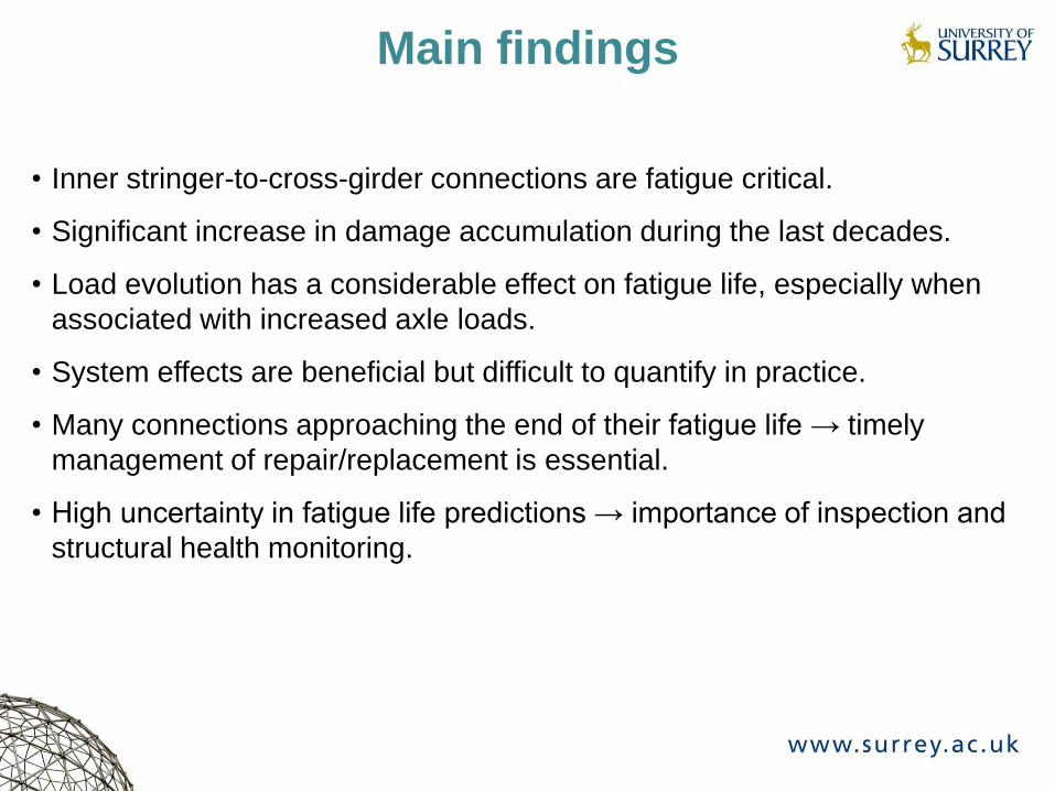
Main findings
• Inner stringer-to-cross-girder connections are fatigue critical.
• Significant increase in damage accumulation during the last decades.
• Load evolution has a considerable effect on fatigue life, especially when
associated with increased axle loads.
• System effects are beneficial but difficult to quantify in practice.
• Many connections approaching the end of their fatigue life → timely
management of repair/replacement is essential.
• High uncertainty in fatigue life predictions → importance of inspection and
structural health monitoring.
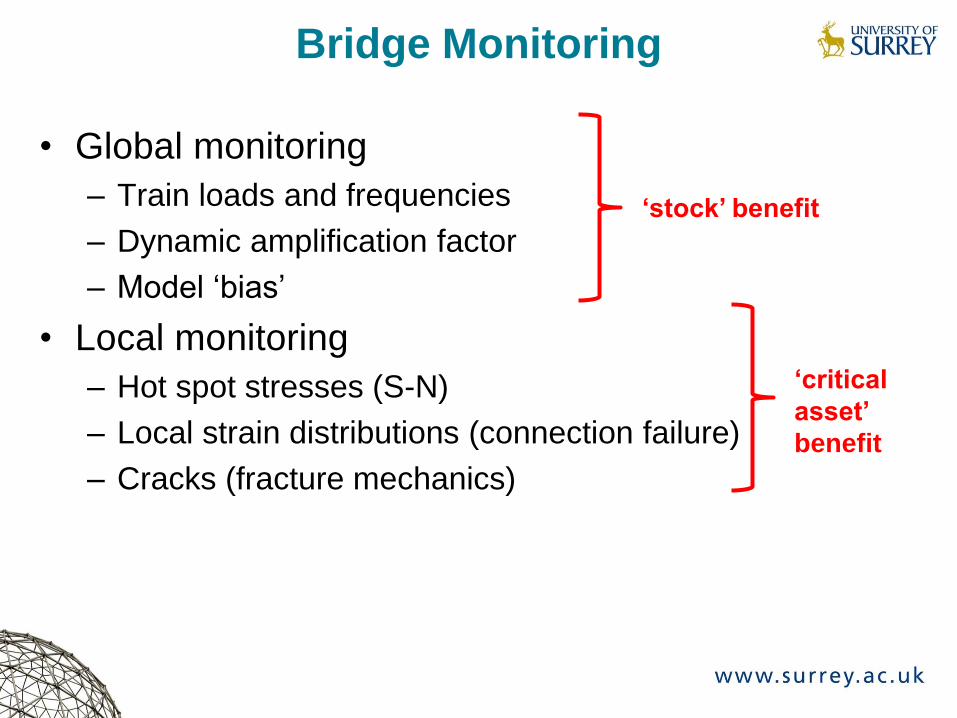
Bridge Monitoring
• Global monitoring
– Train loads and frequencies
– Dynamic amplification factor
– Model ‘bias’
• Local monitoring
– Hot spot stresses (S-N)
– Local strain distributions (connection failure)
– Cracks (fracture mechanics)
‘stock’ benefit
‘critical
asset’
benefit
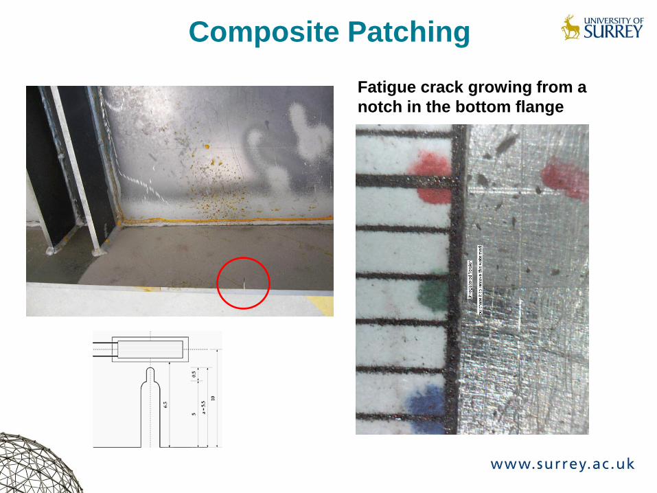
Composite Patching
Fatigue crack growing from a
notch in the bottom flange
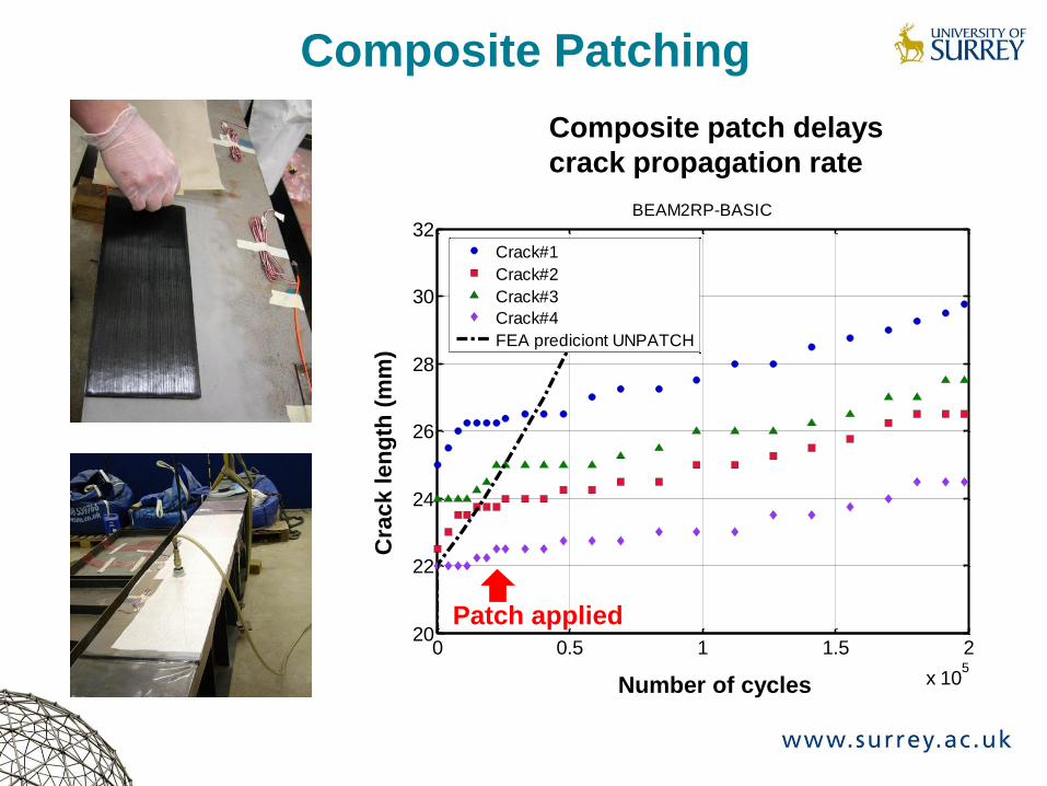
0 0.5 1 1.5 2
x 105
20
22
24
26
28
30
32
Number of cycle
Cra
ck length
[m
m]
BEAM2RP-BASIC
Crack#1
Crack#2
Crack#3
Crack#4
FEA prediciont UNPATCH
Composite patch delays
crack propagation rate
Composite Patching
Number of cycles
Cra
ck l
en
gth
(m
m)
Patch applied
-60
-55
-50
-45
-40
-35
1530 1535 1540 1545 1550 1555 1560
Wavelength, nm
Inte
ns
ity
, d
B
51,000
-60
-55
-50
-45
-40
-35
1530 1535 1540 1545 1550 1555 1560
Wavelength, nm
Inte
ns
ity
, d
B
40,000
-60
-55
-50
-45
-40
-35
1530 1535 1540 1545 1550 1555 1560
Wavelength, nm
Inte
ns
ity
, d
B
34,000
Incr
easi
ng C
ycl
es
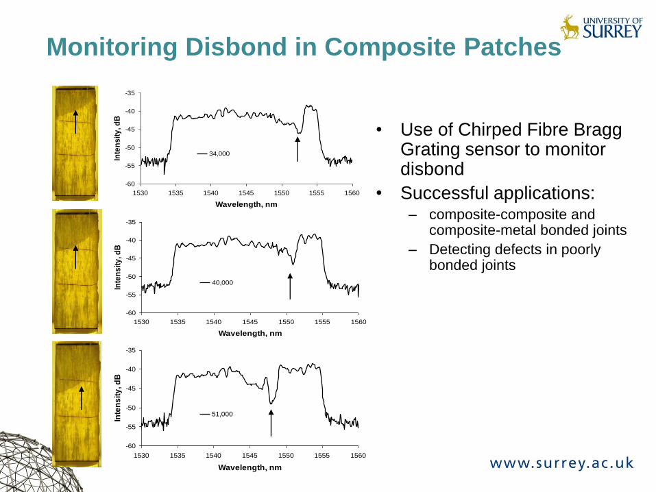
• Use of Chirped Fibre Bragg Grating sensor to monitor disbond
• Successful applications: – composite-composite and
composite-metal bonded joints
– Detecting defects in poorly bonded joints
Monitoring Disbond in Composite Patches
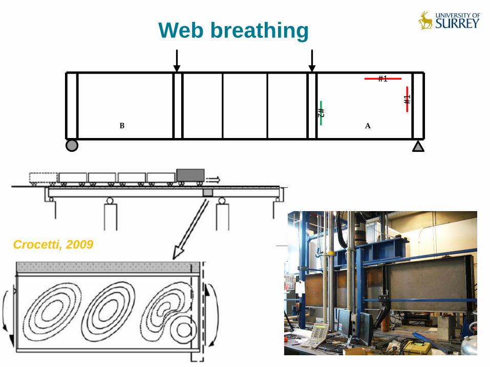
#1#2
AB
#1
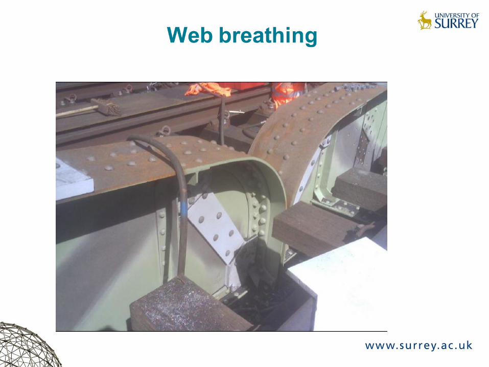
Web breathing
Crocetti, 2009
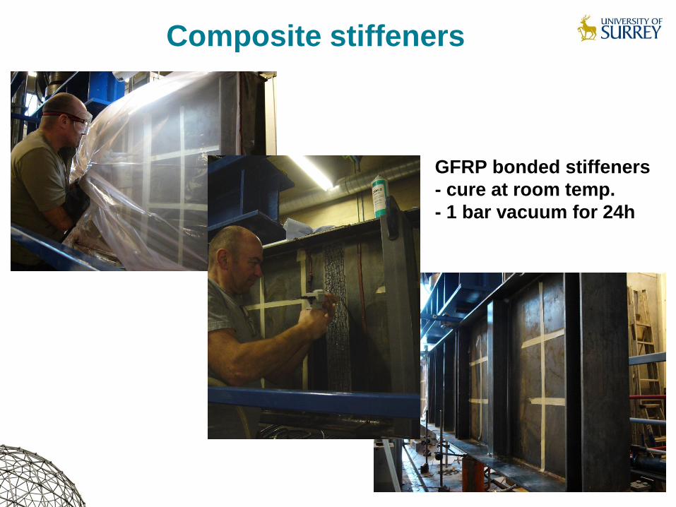
GFRP bonded stiffeners
- cure at room temp.
- 1 bar vacuum for 24h
Composite stiffeners
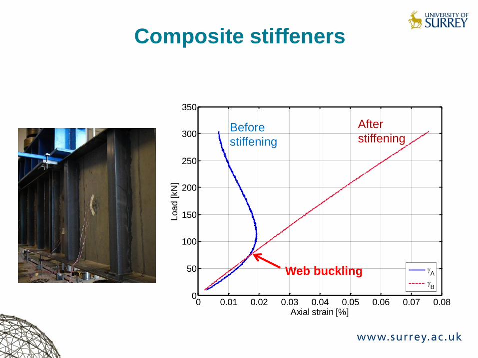
0 0.01 0.02 0.03 0.04 0.05 0.06 0.07 0.080
50
100
150
200
250
300
350
Axial strain [%]
Load [kN
]
A
B
Composite stiffeners
Before
stiffening
After
stiffening
Web buckling
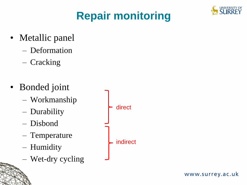
Repair monitoring
• Metallic panel
– Deformation
– Cracking
• Bonded joint
– Workmanship
– Durability
– Disbond
– Temperature
– Humidity
– Wet-dry cycling
direct
indirect
4
3
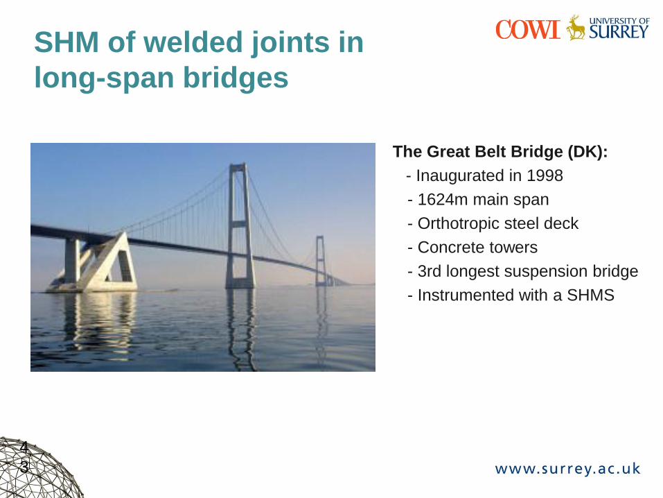
The Great Belt Bridge (DK):
› - Inaugurated in 1998
- 1624m main span
- Orthotropic steel deck
- Concrete towers
- 3rd longest suspension bridge
- Instrumented with a SHMS
SHM of welded joints in
long-span bridges
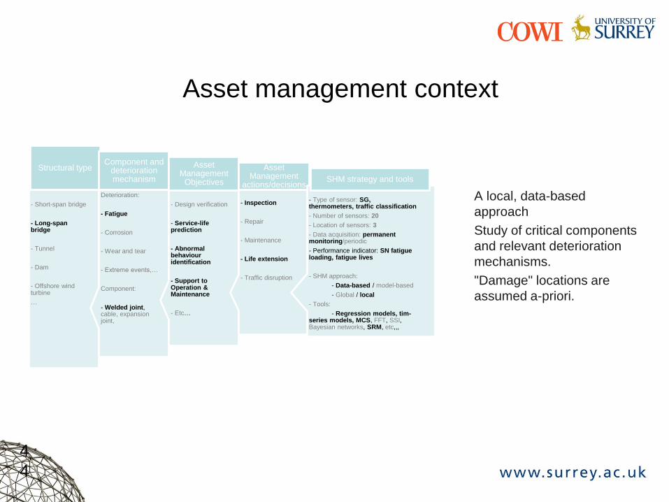
Asset management context
4
4
- Short-span bridge
- Long-span bridge
- Tunnel
- Dam
- Offshore wind turbine
…
Structural type
Deterioration:
- Fatigue
- Corrosion
- Wear and tear
- Extreme events,…
Component:
- Welded joint, cable, expansion joint,
Component and deterioration mechanism
- Design verification
- Service-life prediction
- Abnormal behaviour identification
- Support to Operation & Maintenance
- Etc…
Asset Management
Objectives
- Inspection
- Repair
- Maintenance
- Life extension
- Traffic disruption
Asset Management
actions/decisions
- Type of sensor: SG, thermometers, traffic classification
- Number of sensors: 20
- Location of sensors: 3
- Data acquisition: permanent monitoring/periodic
- Performance indicator: SN fatigue loading, fatigue lives
- SHM approach:
- Data-based / model-based
- Global / local
- Tools:
- Regression models, tim-series models, MCS, FFT, SSI, Bayesian networks, SRM, etc,,,
SHM strategy and tools
› A local, data-based
approach
› Study of critical components
and relevant deterioration
mechanisms.
› "Damage" locations are
assumed a-priori.
4
5
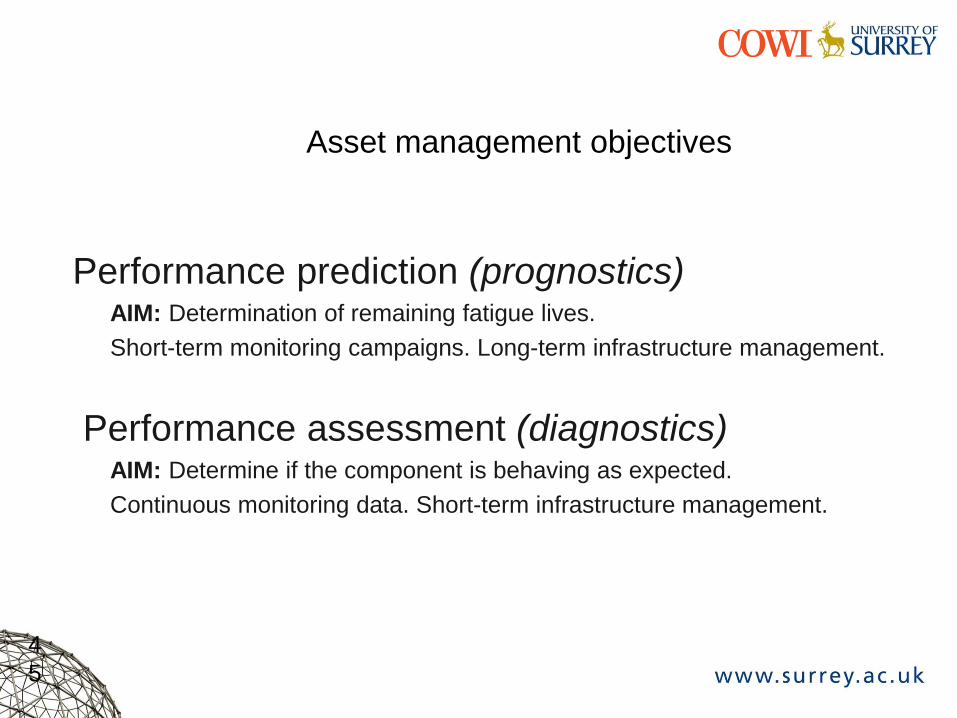
Asset management objectives
›Performance prediction (prognostics) › AIM: Determination of remaining fatigue lives.
› Short-term monitoring campaigns. Long-term infrastructure management.
› Performance assessment (diagnostics) › AIM: Determine if the component is behaving as expected.
› Continuous monitoring data. Short-term infrastructure management.
data interpretation)
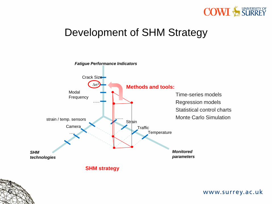
Development of SHM Strategy
4
6
Fatigue Performance Indicators
Crack Size
Ds3
Modal
Frequency …..
Monitored
parameters SHM
technologies
…… Strain
Traffic Temperature
Camera
strain / temp. sensors
….
Methods and tools:
› Time-series models
› Regression models
› Statistical control charts
› Monte Carlo Simulation
SHM strategy
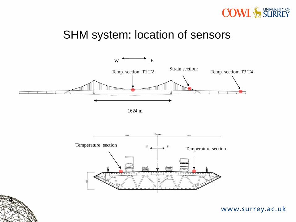
SHM system: location of sensors
4
7
Temp. section: T1,T2 Temp. section: T3,T4
E W
Strain section:
1624 m
Temperature section Temperature section

Focus: welded joints of the orthotropic deck
4
8
trough-to-deck weld
trough splice weld
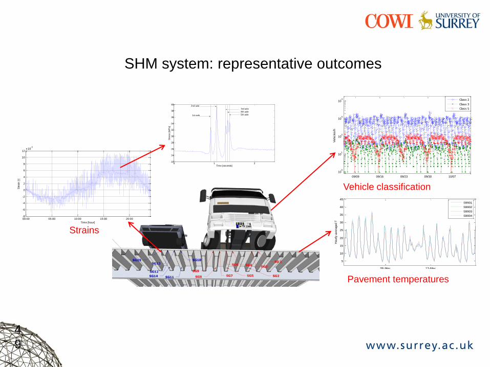
SHM system: representative outcomes
4
9
06-May 13-May
5
10
15
20
25
30
35
40
45
Date
Hourly-a
vera
ged T
S9901
S9902
S9903
S9904
Pavement temperatures
09/09 09/16 09/23 09/30 10/07
100
101
102
103
104
Date
Vehic
les/h
Class 2
Class 3
Class 5
Vehicle classification
00:00 05:00 10:00 15:00 20:00-8
-6
-4
-2
0
2
4
6
8
10
12x 10
-5
Time [hour]
Str
ain
[-]
Strains
0 1 222
24
26
28
30
32
34
36
38
40
Time [seconds]
Str
ess [
MP
a]
2nd axle
1st axle
3rd axle4th axle5th axle
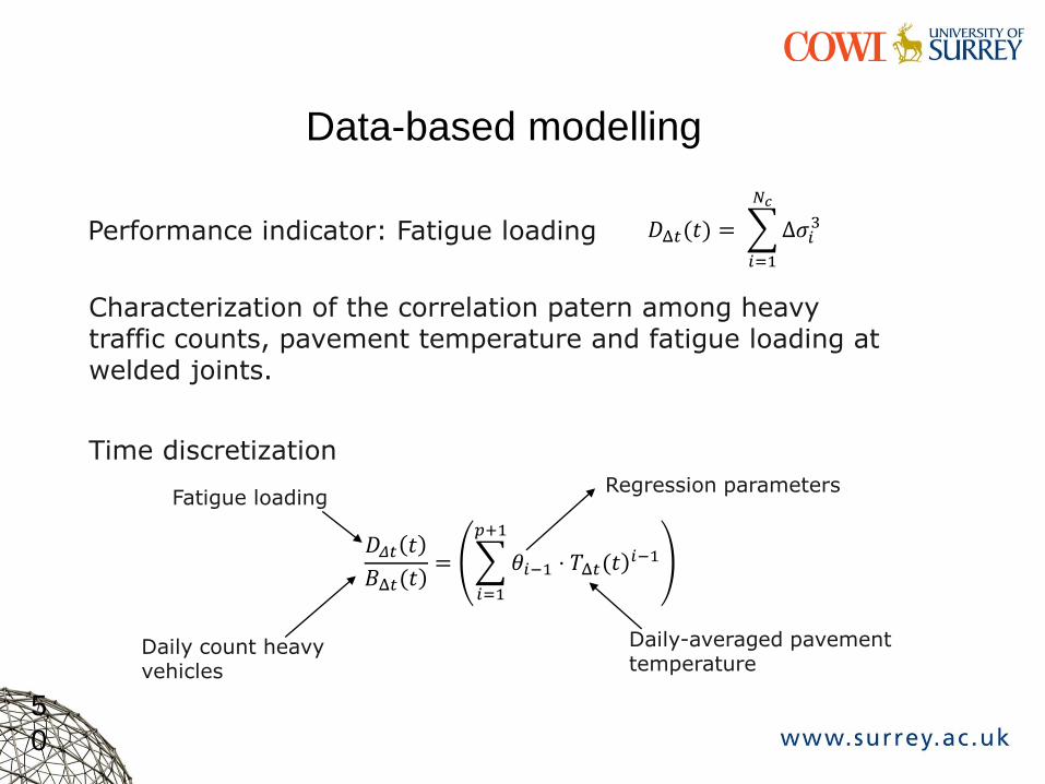
Data-based modelling
5
0
𝐷Δ𝑡(𝑡) = Δ𝜎𝑖3
𝑁𝑐
𝑖=1
› Performance indicator: Fatigue loading
› Characterization of the correlation patern among heavy traffic counts, pavement temperature and fatigue loading at welded joints.
› Time discretization
Daily count heavy vehicles
𝐷𝛥𝑡 𝑡
𝐵Δ𝑡(𝑡)= 𝜃𝑖−1
𝑝+1
𝑖=1
⋅ 𝑇Δ𝑡(𝑡)𝑖−1
Fatigue loading
Daily-averaged pavement temperature
Regression parameters
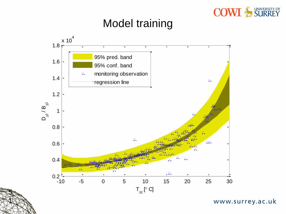
Model training
5
1
-10 -5 0 5 10 15 20 25 300.2
0.4
0.6
0.8
1
1.2
1.4
1.6
1.8x 10
4
TDt
[ C]
DD
t / B
Dt
95% pred. band
95% conf. band
monitoring observation
regression line
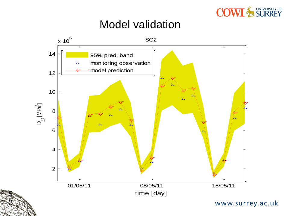
01/05/11 08/05/11 15/05/11
2
4
6
8
10
12
14
x 106
time [day]
DD
t [MP
a3 ]SG2
95% pred. band
monitoring observation
model prediction
Model validation
5
2
5
3
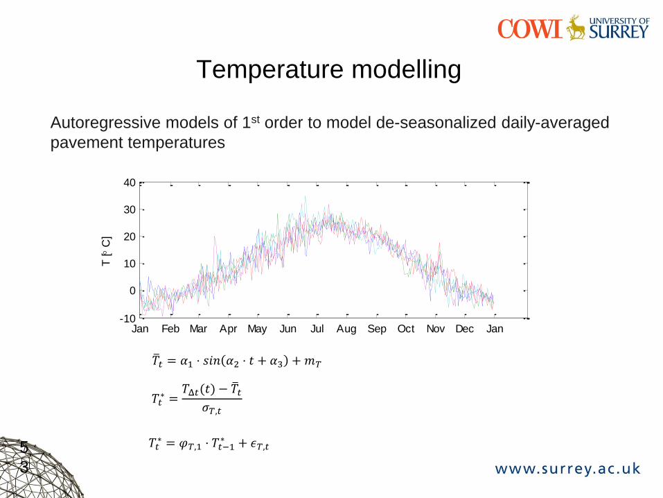
Temperature modelling
› Autoregressive models of 1st order to model de-seasonalized daily-averaged
pavement temperatures Jan Feb Mar Apr May Jun Jul Aug Sep Oct Nov Dec Jan-10
0
10
20
30
40
T [
C]
Jan Feb Mar Apr May Jun Jul Aug Sep Oct Nov Dec Jan-10
0
10
20
30
40
T [
C]
𝑇 𝑡 = 𝛼1 ⋅ 𝑠𝑖𝑛 𝛼2 ⋅ 𝑡 + 𝛼3 +𝑚𝑇
𝑇𝑡∗ =𝑇Δ𝑡(𝑡) − 𝑇 𝑡𝜎𝑇,𝑡
𝑇𝑡∗ = 𝜑𝑇,1 ⋅ 𝑇𝑡−1
∗ + 𝜖𝑇,𝑡
5
4
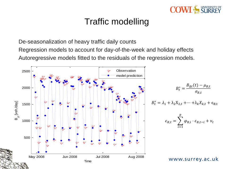
𝐵𝑡∗ =𝐵Δ𝑡(𝑡) − 𝜇𝐵,𝑡𝜎𝐵,𝑡
Traffic modelling
› De-seasonalization of heavy traffic daily counts
› Regression models to account for day-of-the-week and holiday effects
› Autoregressive models fitted to the residuals of the regression models.
May 2008 Jun 2008 Jul 2008 Aug 2008
500
1000
1500
2000
2500
BD
t [veh./day]
Time
Observation
model prediction
𝐵𝑡∗ = 𝜆1 + λ2X2,𝑡 +⋅⋅⋅ +λ𝑘𝑋𝑘,𝑡 + ϵB,t
𝜖𝐵,𝑡 = 𝜑𝐵,𝑖 ⋅ 𝜖𝐵,𝑡−𝑖
𝑝
𝑖=1
+ 𝜈𝑡

Application 1: Fatigue life prediction
5
5
55 0 100 200 300 400 500 600 700 800 900 1000
0
2000
4000
6000
8000
10000
12000
Monte Carlo Simulation
t f [years
]
102
103
104
105
0.0005
0.005
0.05
0.25
0.5
0.75
0.95
0.995
0.9995
Data
Pro
bability
0 100 200 300 400 500 600 700 800-20
0
20
40
T24h [ C
]
0 100 200 300 400 500 600 700 8000
1000
2000
3000
4000
B24h [veh./h]
0 100 200 300 400 500 600 700 8000
2
4
6
8
10
12
14x 10
6
D24h [M
Pa3
]
Time [days]
0 100 200 300 400 500 600 700 800-20
0
20
40
T24h [ C
]
0 100 200 300 400 500 600 700 8000
1000
2000
3000
4000
B24h [veh./h]
0 100 200 300 400 500 600 700 8000
2
4
6
8
10
12
14x 10
6
D24h [M
Pa3
]
Time [days]
0 100 200 300 400 500 600 700 800-20
0
20
40
T24h [ C
]
0 100 200 300 400 500 600 700 8000
1000
2000
3000
4000
B24h [veh./h]
0 100 200 300 400 500 600 700 8000
2
4
6
8
10
12
14x 10
6
D24h [M
Pa3
]
Time [days]
Simulation of actions, i.e. traffic and temperature
(time-series models)
Simulation of fatigue loading
(regression models) Monte Carlo simulation: time to failure
realizations (S-N LSF)
0 50 100 1502
4
6
8
10
12
14
Time [years]
SG 1
SG 3
SG 4
SG 6
SG 7
SG 9
*=3.8
Fatigue life prediction
(reliability profile)
Application 1: Fatigue life prediction
5
6
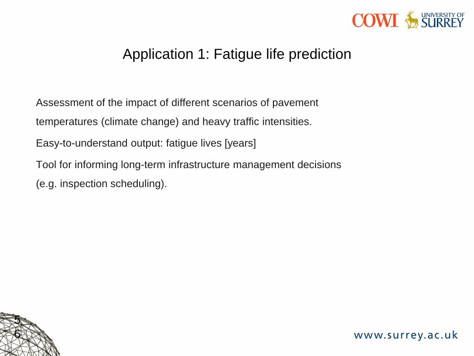
› Assessment of the impact of different scenarios of pavement
temperatures (climate change) and heavy traffic intensities.
› Easy-to-understand output: fatigue lives [years]
› Tool for informing long-term infrastructure management decisions
(e.g. inspection scheduling).
Application 2: Performance assessment
5
7
04/29 05/06 05/13 05/20
-6
-4
-2
0
2
4
6
Norm
aliz
ed r
esid
uals
99 % LCL
99 %UCL
15/05/2012
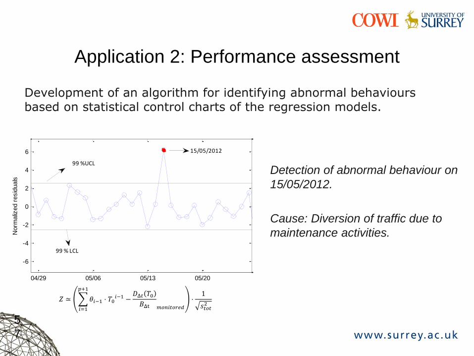
› Detection of abnormal behaviour on
15/05/2012.
› Cause: Diversion of traffic due to
maintenance activities.
› Development of an algorithm for identifying abnormal behaviours based on statistical control charts of the regression models.
𝑍 ≃ 𝜃𝑖−1
𝑝+1
𝑖=1
⋅ 𝑇0𝑖−1 −𝐷Δ𝑡 𝑇0𝐵Δt 𝑚𝑜𝑛𝑖𝑡𝑜𝑟𝑒𝑑
⋅1
𝑠𝑡𝑜𝑡2
Concluding remarks
• SHM should be requirement-pull not technology-push
• SHM strategies depend on the Asset Management
objectives and constraints
• Key for exploitation of SHM in civil structures is the
chain from Data to Information to Knowledge
• Traffic light concept:
Healthy - Concern - Faulty
• Beware of Infobesity "As long as the centuries continue to
unfold, … one can predict that a time will
come when it will be almost as difficult to
learn anything from books as from the
direct study of the whole universe. Diderot,
"Encyclopédie" (1755)