April 2007

NASA/TM-2007-214871

Structural Analysis Methods for Structural Health Management of Future Aerospace Vehicles Alexander Tessler Langley Research Center, Hampton, Virginia

https://ntrs.nasa.gov/search.jsp?R=20070018347 2018-07-23T11:01:15+00:00Z

The NASA STI Program Office . . . in Profile

Since its founding, NASA has been dedicated to the advancement of aeronautics and space science. The NASA Scientific and Technical Information (STI) Program Office plays a key part in helping NASA maintain this important role.

The NASA STI Program Office is operated by Langley Research Center, the lead center for NASA’s scientific and technical information. The NASA STI Program Office provides access to the NASA STI Database, the largest collection of aeronautical and space science STI in the world. The Program Office is also NASA’s institutional mechanism for disseminating the results of its research and development activities. These results are published by NASA in the NASA STI Report Series, which includes the following report types:

• TECHNICAL PUBLICATION. Reports of

completed research or a major significant phase of research that present the results of NASA programs and include extensive data or theoretical analysis. Includes compilations of significant scientific and technical data and information deemed to be of continuing reference value. NASA counterpart of peer-reviewed formal professional papers, but having less stringent limitations on manuscript length and extent of graphic presentations.

• TECHNICAL MEMORANDUM. Scientific

and technical findings that are preliminary or of specialized interest, e.g., quick release reports, working papers, and bibliographies that contain minimal annotation. Does not contain extensive analysis.

• CONTRACTOR REPORT. Scientific and

technical findings by NASA-sponsored contractors and grantees.

• CONFERENCE PUBLICATION. Collected

papers from scientific and technical conferences, symposia, seminars, or other meetings sponsored or co-sponsored by NASA.

• SPECIAL PUBLICATION. Scientific,

technical, or historical information from NASA programs, projects, and missions, often concerned with subjects having substantial public interest.

• TECHNICAL TRANSLATION. English-

language translations of foreign scientific and technical material pertinent to NASA’s mission.

Specialized services that complement the STI Program Office’s diverse offerings include creating custom thesauri, building customized databases, organizing and publishing research results ... even providing videos. For more information about the NASA STI Program Office, see the following: • Access the NASA STI Program Home Page at

http://www.sti.nasa.gov • E-mail your question via the Internet to

help@sti.nasa.gov • Fax your question to the NASA STI Help Desk

at (301) 621-0134 • Phone the NASA STI Help Desk at

(301) 621-0390 • Write to:

NASA STI Help Desk NASA Center for AeroSpace Information 7115 Standard Drive Hanover, MD 21076-1320

National Aeronautics and Space Administration Langley Research Center Hampton, Virginia 23681-2199

April 2007

NASA/TM-2007-214871

Structural Analysis Methods for Structural Health Management of Future Aerospace Vehicles Alexander Tessler Langley Research Center, Hampton, Virginia

Available from: NASA Center for AeroSpace Information (CASI) National Technical Information Service (NTIS) 7115 Standard Drive 5285 Port Royal Road Hanover, MD 21076-1320 Springfield, VA 22161-2171 (301) 621-0390 (703) 605-6000

Abstract

Two finite element based computational methods, Smoothing Element Analysis (SEA) and the inverse Finite Element Method (iFEM), are reviewed, and examples of their use for structural health monitoring are discussed. Due to their versatility, robustness, and computational efficiency, the methods are well suited for real-time structural health monitoring of future space vehicles, large space structures, and habitats. The methods may be effectively employed to enable real-time processing of sensing information, specifically for identifying three-dimensional deformed structural shapes as well as the internal loads. In addition, they may be used in conjunction with evolutionary algorithms to design optimally distributed sensors. These computational tools have demonstrated substantial promise for utilization in future Structural Health Management (SHM) systems.

Introduction

The Integrated Vehicle Health Management (IVHM) research at NASA Langley Research Center explores safe, reliable, and affordable technologies for NASA’s future long duration space missions [1]. Integral to this research is mitigation of aerospace vehicle accidents due to structural failures. For long duration space missions, real-time monitoring of structural, propulsion, thermal protection, and other critical systems will be required. To achieve such capabilities, space vehicles and habitation structures will be designed with diverse arrays of optimally distributed in-situ sensors. The sensing technologies will be part of advanced data systems architectures that will process, communicate, and store massive amounts of SHM data. Special-purpose structural analysis and design algorithms will be necessary to incorporate SHM sensing data for the diagnosis and prognosis of structural integrity, and for the purpose of optimal design and construction of such structures. Structural integrity information will be utilized within an IVHM system, resulting in the safe and effective operational vehicle management and mission control.

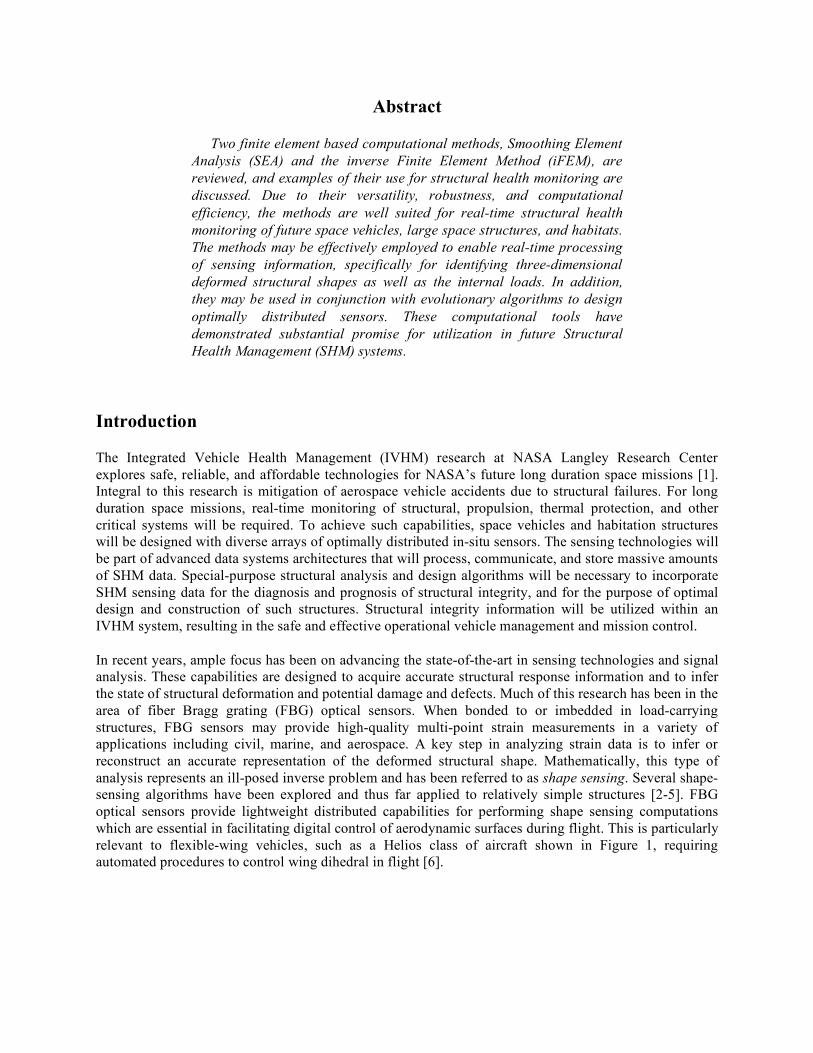
In recent years, ample focus has been on advancing the state-of-the-art in sensing technologies and signal analysis. These capabilities are designed to acquire accurate structural response information and to infer the state of structural deformation and potential damage and defects. Much of this research has been in the area of fiber Bragg grating (FBG) optical sensors. When bonded to or imbedded in load-carrying structures, FBG sensors may provide high-quality multi-point strain measurements in a variety of applications including civil, marine, and aerospace. A key step in analyzing strain data is to infer or reconstruct an accurate representation of the deformed structural shape. Mathematically, this type of analysis represents an ill-posed inverse problem and has been referred to as shape sensing. Several shape-sensing algorithms have been explored and thus far applied to relatively simple structures [2-5]. FBG optical sensors provide lightweight distributed capabilities for performing shape sensing computations which are essential in facilitating digital control of aerodynamic surfaces during flight. This is particularly relevant to flexible-wing vehicles, such as a Helios class of aircraft shown in Figure 1, requiring automated procedures to control wing dihedral in flight [6].

2

Figure 1. Helios solar powered aircraft during first flight on July 14, 2001 at Dryden Flight Research Center, California.

In general, the class of Unmanned Aerial Vehicles (UAV) may derive substantial performance benefits using real-time wing surface control systems. For large space structures, including solar sails and membrane antennas, knowing the current three-dimensional shape of the structure may maximize spacecraft performance [7-8].

This paper reviews two notable full-field computational algorithms, known as SEA [9-10] and iFEM [4-5]. The methods combine the attributes of computational efficiency, versatility, and robustness that are necessary for real-time, large-scale SHM applications. The algorithms may serve as both design tools for the development of optimal sensing systems and enabling tools for the processing of sensing information in real time. Following the mathematical description of SEA and iFEM and discussions of their salient features, several SHM applications of the two methods are highlighted. These include (1) shape sensing and structural anomaly detection in beam structures instrumented with FBG sensors, (2) identification of delamination damage in composite laminates, and (3) design of optimal strain sensor locations.

Smoothing Element Analysis

Smoothing Element Analysis (SEA) provides a robust and versatile computational capability for smoothing discrete data of either experimental or numerical origin that are defined over arbitrary geometric domains. In addition to obtaining smooth fields, the method computes smooth first-order derivatives of the field of interest. SEA is a finite element method derived on the basis of a Penalized Discrete Least Squares (PDLS) variational principle. The method treats any discrete data as corresponding to a scalar quantity.

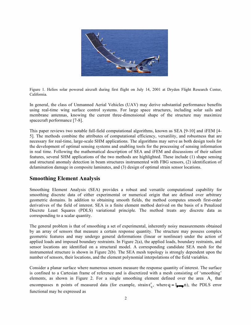
The general problem is that of smoothing a set of experimental, inherently noisy measurements obtained by an array of sensors that measure a certain response quantity. The structure may possess complex geometric features and may undergo general deformations (linear or nonlinear) under the action of applied loads and imposed boundary restraints. In Figure 2(a), the applied loads, boundary restraints, and sensor locations are identified on a structural model. A corresponding candidate SEA mesh for the instrumented structure is shown in Figure 2(b). The SEA mesh topology is strongly dependent upon the number of sensors, their locations, and the element polynomial interpolations of the field variables.

Consider a planar surface where numerous sensors measure the response quantity of interest. The surface is confined to a Cartesian frame of reference and is discretized with a mesh consisting of ‘smoothing’ elements, as shown in Figure 2. For a single smoothing element defined over the area

!

Ae that

encompasses

!

n points of measured data (for example, strain

!

"q" , where

!

q =1, ...,n), the PDLS error functional may be expressed as

3

!

"e =1

nq=1

n

# [$q$ % $(xq )]

2 + & [ ($, x %'x )2 + ($, y %'y )

2] dxdyAe(

+ )Ae [('x, x )2 + ('y, y )

2 +Ae( 1

2('x, y + 'y, x )

2] dxdy (1)

where

!

"(xq ) a smooth strain is interpolated over the element and evaluated at the sensor position

!

xq = (xq , yq ) ;

!

"x and

!

"y are independent variables that, respectively, approach very closely the partial

derivatives

!

", x and

!

",y (refer to Eqs. (2)). In general, the symbol

!

" may represent an arbitrary quantity of interest, e.g., displacement or temperature. For superior numerical accuracy, the complete array of measured data must be normalized with respect to its maximum magnitude.

The first term in Eq. (1) is weighted least squares with the weighting coefficient defined as the inverse of the number of sensors (obviously, other normalization options exist). Thus, the measured data are weighted equally within an element. The second term in Eq. (1) is a penalty constraint functional which, for a relatively large value of the dimensionless parameter

!

" (~106), ensures the limiting condition of

!

C1

continuity for

!

",

!

", x #$x and ", y #$y in Ae (2)

where it is assumed that

!

",

!

"x and

!

"y are interpolated using

!

C0-continuous shape functions. The third

term in Eq. (1) is a regularization function in which β is a positive regularization parameter. Assigning small values of β (~10-6) provides additional constraint conditions for the

!

"x and

!

"y variables. This yields nonsingular least squares equations even when some elements do not encompass any sensors or data.

In accordance with the standard finite element procedures, the total PDLS error functional is computed as the sum of all element contributions and is minimized with respect to the nodal degrees-of-freedom associated with the

!

",

!

"x, and

!

"y variables. The resulting linear equations are factorized, yielding point-wise smooth solutions for these variables.

Figure 2. (a) A schematic of a structural model showing the load, boundary restraints, and sensor locations, (b) SEA mesh discretizing the structural model and encompassing the sensor positions.

4

The practical aspects of applying SEA include: (1) boundary conditions may be imposed on both the smoothed quantity

!

" and the variables,

!

"x, and

!

"y , thus taking advantage of certain physical conditions that are known a priori, (2) higher-order derivatives of the measured quantity can be computed by applying the method sequentially in multiple steps, and (3) multiple sets of data may be smoothed efficiently, especially when the data are measured at the same sensor locations (e.g., three strain components measured by strain rosettes). For such cases, an efficient factorization algorithm of linear equations with multiple right-hand sides is required.

Inverse Finite Element Method

The iFEM has been developed for plate and shell structures [4-5] and is readily reduced to beams and frames. The method is formulated for the purposes of (1) reconstructing a smooth displacement field from strain data measured by in-situ strain sensors, and (2) computing the full-field strain, stress, and internal load (stress resultant) fields using the reconstructed displacement field. This part of the analysis follows the same basic procedures of the forward (direct) FEM.

The first (and primary) part of iFEM performs a smoothing operation of all components of measured strain simultaneously. This requires all strain-tensor relations pertinent to the analytic theory be incorporated in the formulation. The iFEM formulation is based upon minimization of a least squares functional that uses Mindlin theory assumptions. The error functional for an inverse shell element of area

!

Ae that encompasses

!

n strain-sensor locations may be stated as

!

"e

#(u) = e u( ) $e%

2

+ k u( ) $k%2

+ # g u( ) $g%2

(3)

where the squared norms are least-squares difference terms defined as

( )2 2

1

1( ) x y

e

n

i iAi

d dn

! !

=

" #$ % $& '()e u e e u e

( )2

2 2

1

(2 )( ) x y

e

n

i iAi

td d

n

! !

=

" #$ % $& '()k u k k u k (4)

( )2 2

1

1( ) x y

e

n

i iAi

d dn

! !

=

" #$ % $& '()g u g g u g

and

!

" (~10-6) denotes a dimensionless regularization parameter. The strain measures are defined in a customary manner in terms of

!

C0-continuous kinematic variables

!

uT = u, v, w, "x , "y{ } as

!

e u( )T

= u, x , v, y , "x, y + "y, x{ } (In-plane strains)

!

k u( )T

= "y, x , "x, y , "x, x + "y, y{ } (Curvatures) (5)

!

g u( )T

= w , x + "y , w , y + "x{ } (Transverse shear strains)

5

where

!

u = u(x, y) and

!

v = v(x, y) are the mid-plane displacements in the

!

x and

!

y directions, respectively;

!

"x = "x (x, y) and

!

"y = "y (x, y) are the rotations of the normal about the negative

!

x and positive

!

y axes, respectively; and

!

w =w(x, y) is the deflection variable which is constant across the thickness coordinate

!

z " [#t, t] , with 2t denoting the shell thickness.

The

!

e" and

!

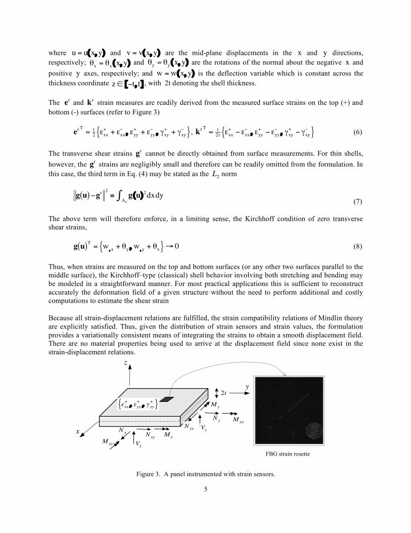
k" strain measures are readily derived from the measured surface strains on the top (+) and

bottom (-) surfaces (refer to Figure 3)

!

e"T = 1

2"xx

+ + "xx# , "yy

+ + "yy# , $xy

+ + $xy#{ },

!

k"T = 1

2t"xx

+ # "xx# , "yy

+ # "yy# , $xy

+ # $xy#{ } (6)

The transverse shear strains

!

g" cannot be directly obtained from surface measurements. For thin shells,

however, the

!

g" strains are negligibly small and therefore can be readily omitted from the formulation. In

this case, the third term in Eq. (4) may be stated as the

!

L2 norm

!

g u( ) "g#2

$ g(u)2dxAe% dy

(7)

The above term will therefore enforce, in a limiting sense, the Kirchhoff condition of zero transverse shear strains,

!

g u( )T

= w , x + "y , w , y + "x{ }# 0 (8)

Thus, when strains are measured on the top and bottom surfaces (or any other two surfaces parallel to the middle surface), the Kirchhoff–type (classical) shell behavior involving both stretching and bending may be modeled in a straightforward manner. For most practical applications this is sufficient to reconstruct accurately the deformation field of a given structure without the need to perform additional and costly computations to estimate the shear strain

Because all strain-displacement relations are fulfilled, the strain compatibility relations of Mindlin theory are explicitly satisfied. Thus, given the distribution of strain sensors and strain values, the formulation provides a variationally consistent means of integrating the strains to obtain a smooth displacement field. There are no material properties being used to arrive at the displacement field since none exist in the strain-displacement relations.

Figure 3. A panel instrumented with strain sensors.

!

"xx+ , "yy

+ , # xy+{ }

!

x

!

y

!

2t!

z

!

Ny

!

My

!

Vy

!

Nyx

!

Myx

!

Vx

!

Nxy

!

Mxy

!

Mx

!

Nx

FBG strain rosette

6

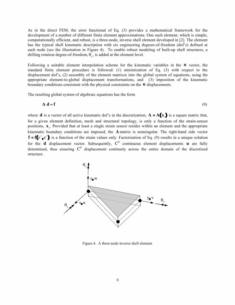
As in the direct FEM, the error functional of Eq. (3) provides a mathematical framework for the development of a number of different finite element approximations. One such element, which is simple, computationally efficient, and robust, is a three-node, inverse shell element developed in [2]. The element has the typical shell kinematic description with six engineering degrees-of-freedom (dof’s) defined at each node (see the illustration in Figure 4). To enable robust modeling of built-up shell structures, a drilling rotation degree-of-freedom,

!

"z, is added at the element level.

Following a suitable element interpolation scheme for the kinematic variables in the

!

u vector, the standard finite element procedure is followed: (1) minimization of Eq. (3) with respect to the displacement dof’s, (2) assembly of the element matrices into the global system of equations, using the appropriate element-to-global displacement transformations, and (3) imposition of the kinematic boundary conditions consistent with the physical constraints on the

!

u displacements.

The resulting global system of algebraic equations has the form

!

A d = f (9)

where

!

d is a vector of all active kinematic dof’s in the discretization;

!

A "A(xi) is a square matrix that,

for a given element definition, mesh and structural topology, is only a function of the strain-sensor positions,

!

xi. Provided that at least a single strain sensor resides within an element and the appropriate

kinematic boundary conditions are imposed, the

!

Amatrix is nonsingular. The right-hand side vector

!

f " f(#+ ,#$) is a function of the strain values only. Factorization of Eq. (9) results in a unique solution for the

!

d displacement vector. Subsequently,

!

C0 continuous element displacements

!

u are fully determined, thus ensuring

!

C0 displacement continuity across the entire domain of the discretized

structure.

Figure 4. A three-node inverse shell element.

!

"x

!

"y

!

"z

!

z,w

!

x,u

!

y, v

7

Full-Field Strains and Internal Loads

Once the element displacement field

!

u is obtained, the element level ‘recovery’ of strains, stresses and stress resultants follows standard finite element procedures. First, the in-plane and curvature strain measures are computed from Eqs. (5), leading to the computation of the strains

!

"xx , "yy , #xy{ }T

$ e u( ) + z k u( ) (10)

Assuming linear elastic behavior, the stresses

!

" # "xx , "yy , $xy{ }T

are obtained from the stress-strain relations

!

" #D $xx , $yy , %xy{ }T

(11)

The stress resultants

!

R " Nx , Ny , Nxy , Mx , My , Mxy{ }T

are computed from the constitutive relations that involve the strain measures (see Figure 3)

!

R "Qe

k

# $ %

& ' (

(12)

where

!

D and

!

Q are the appropriate constitutive matrices. The transverse shear forces can then be calculated from the equilibrium equations of plate theory,

!

Vx =Mx, x +Mxy, y and Vy =Mxy, x +My, y (13)

Computational Speed and Real-Time Applications

The issue of computational speed is paramount for real-time applications. An on-board computer should be able to perform the computational tasks fast enough to provide the requisite response data to an automated control system and the pilot visualization display. The special features of iFEM appear perfectly suited for such an environment. The iFEM computational paradigm is as follows. The iFEM structural model of an aerospace structure is fully defined in terms of its geometry, discretization by the inverse finite elements, the displacement boundary conditions, and the strain sensors positions. Since the system matrix

!

A is a function of the strain-sensor positions only, the matrix is inverted once and for all, and remains unchanged during the operation of the vehicle. Thus, only the right-hand side vector

!

f is recomputed in real time (since the measured strains change during flight) followed by the fast dot-product operation

!

d =A"1f (14)

The displacement data

!

d (i.e., the deformed shape) is then fed into an automated control system to perform the necessary control-surface adjustments consistent with the current deformed shape of the structure, e.g., a wing. Furthermore, the recovered internal loads, computed according to Eqs. (11)-(13),

8

may be displayed on the pilot’s monitor to ascertain the current internal loads environment on the vehicle. Using the internal loads information, appropriate failure criteria may be calculated, stored, and displayed in real-time.

Meshing Strategies and Optimization of Sensor Locations

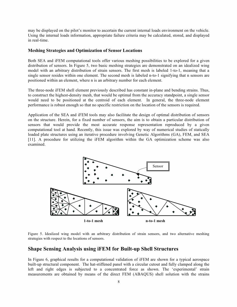
Both SEA and iFEM computational tools offer various meshing possibilities to be explored for a given distribution of sensors. In Figure 5, two basic meshing strategies are demonstrated on an idealized wing model with an arbitrary distribution of strain sensors. The first mesh is labeled 1-to-1, meaning that a single sensor resides within one element. The second mesh is labeled n-to-1 signifying that n sensors are positioned within an element, where n is an arbitrary number for each element.

The three-node iFEM shell element previously described has constant in-plane and bending strains. Thus, to construct the highest-density mesh, that would be optimal from the accuracy standpoint, a single sensor would need to be positioned at the centroid of each element. In general, the three-node element performance is robust enough so that no specific restriction on the location of the sensors is required.

Application of the SEA and iFEM tools may also facilitate the design of optimal distribution of sensors on the structure. Herein, for a fixed number of sensors, the aim is to obtain a particular distribution of sensors that would provide the most accurate response representation reproduced by a given computational tool at hand. Recently, this issue was explored by way of numerical studies of statically loaded plate structures using an iterative procedure involving Genetic Algorithms (GA), FEM, and SEA [11]. A procedure for utilizing the iFEM algorithm within the GA optimization scheme was also examined.

Figure 5. Idealized wing model with an arbitrary distribution of strain sensors, and two alternative meshing strategies with respect to the locations of sensors.

Shape Sensing Analysis using iFEM for Built-up Shell Structures

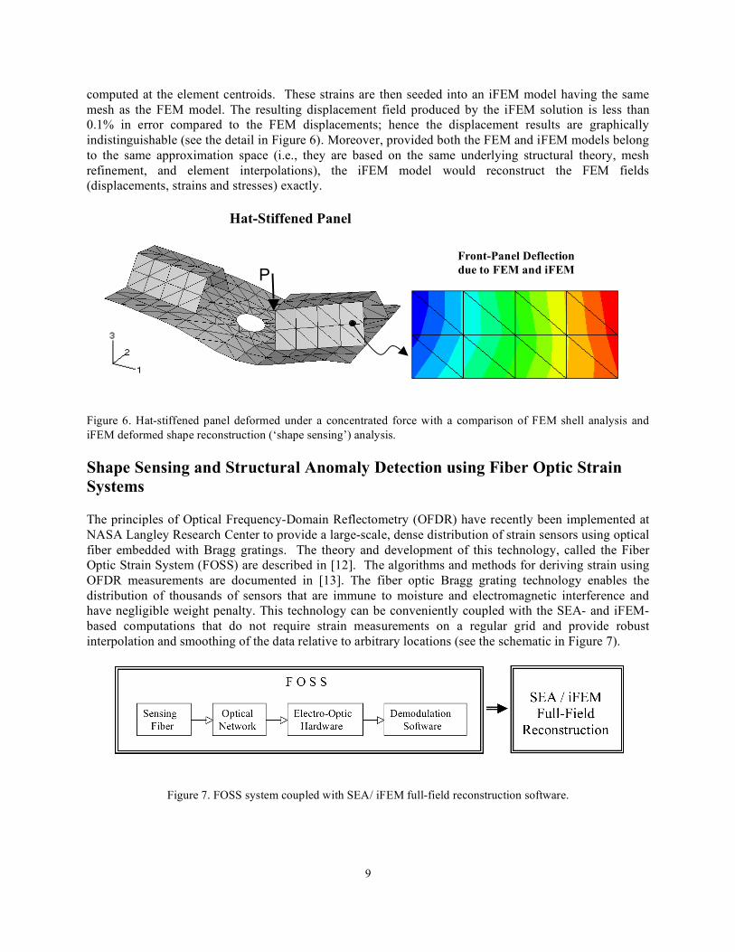
In Figure 6, graphical results for a computational validation of iFEM are shown for a typical aerospace built-up structural component. The hat-stiffened panel with a circular cutout and fully clamped along the left and right edges is subjected to a concentrated force as shown. The ‘experimental’ strain measurements are obtained by means of the direct FEM (ABAQUS) shell solution with the strains

Sensor

1-to-1 mesh n-to-1 mesh

9

computed at the element centroids. These strains are then seeded into an iFEM model having the same mesh as the FEM model. The resulting displacement field produced by the iFEM solution is less than 0.1% in error compared to the FEM displacements; hence the displacement results are graphically indistinguishable (see the detail in Figure 6). Moreover, provided both the FEM and iFEM models belong to the same approximation space (i.e., they are based on the same underlying structural theory, mesh refinement, and element interpolations), the iFEM model would reconstruct the FEM fields (displacements, strains and stresses) exactly.

Figure 6. Hat-stiffened panel deformed under a concentrated force with a comparison of FEM shell analysis and iFEM deformed shape reconstruction (‘shape sensing’) analysis.

Shape Sensing and Structural Anomaly Detection using Fiber Optic Strain Systems

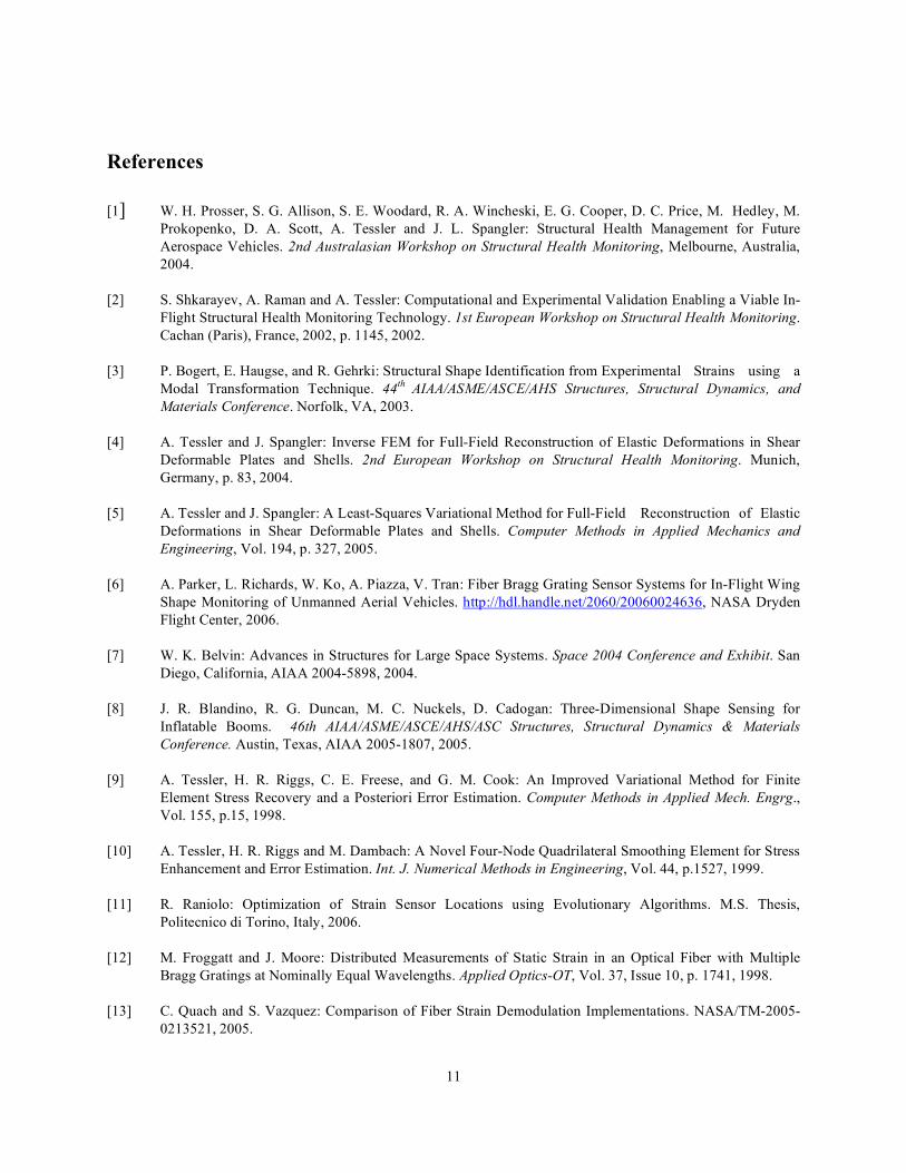
The principles of Optical Frequency-Domain Reflectometry (OFDR) have recently been implemented at NASA Langley Research Center to provide a large-scale, dense distribution of strain sensors using optical fiber embedded with Bragg gratings. The theory and development of this technology, called the Fiber Optic Strain System (FOSS) are described in [12]. The algorithms and methods for deriving strain using OFDR measurements are documented in [13]. The fiber optic Bragg grating technology enables the distribution of thousands of sensors that are immune to moisture and electromagnetic interference and have negligible weight penalty. This technology can be conveniently coupled with the SEA- and iFEM-based computations that do not require strain measurements on a regular grid and provide robust interpolation and smoothing of the data relative to arbitrary locations (see the schematic in Figure 7).

Figure 7. FOSS system coupled with SEA/ iFEM full-field reconstruction software.

P Front-Panel Deflection due to FEM and iFEM

Hat-Stiffened Panel

10

The FOSS and iFEM technologies were successfully applied to a series of laboratory tests conducted on an aluminum bar undergoing bending deformations [14,15]. The first study focused on recovering the correct deformed shape (i.e., shape sensing analysis) of a beam based upon the discrete strain measurements provided by the FOSS system. In the second study, the aim was to detect structural anomalies represented by open holes. The objective was to identify structural anomalies that result in observable changes in localized strain but do not impact the overall surface shape. The iFEM analyses provided the full-field displacements and internal loads using strain data from in-situ fiber-optic sensors. Issues related to improvements in sensor application techniques and optimal levels of sensor density and layout schemes are yet to be investigated.

Identification of Delamination Damage in Composite Plates

In a recent computational study, a non-destructive detection of delamination damage in composite plates was addressed using high-frequency dynamic excitations [16]. The structural response was modeled by the finite element method using Mindlin-type plate elements. The approach does not require vibration measurements on the undamaged structure. The principal parameter used in assessing the state of delamination damage is the curvature tensor of the damaged structure. Once properly analyzed, the complete curvature tensor provides useful information for identifying the location and size of delaminations.

The smoothed curvature data, corresponding to the high-frequency modes, serve as a measure of comparison for the raw mode-shape data that are obtained for a damaged structure. Whereas the modal shapes of the undamaged plate are presumed to be unavailable, the smoothed curvatures obtained via SEA provide the proper reference curvature fields. The implementation of a damage identification procedure then involves the full-field assessment of a suitable damage indicator.

Effects of random error in the curvature data were also studied to ascertain the sensitivity of the method to noisy experimental data. The approach led to reasonably good predictions of the delamination shape and location even near the panel boundaries.

Conclusions

Two finite element based computational methods, SEA and iFEM, were reviewed and their salient features discussed in relation to SHM systems for use in future spacecraft, large space structures, and habitation structures. The methods and their associate algorithms satisfy the key requirements for use in real-time, large-scale structural applications, i.e., versatility, robustness, and computational efficiency. Several recent research efforts in which SEA and iFEM played a key role were also highlighted. These include computational and experimental studies of reconstructing, based on in-situ strain measurements, structural deformations (i.e., ‘shape sensing’), identification of structural anomalies including delamitations in composite laminates, and sensor-position optimization studies employing genetic algorithms. The iFEM capability also permits reconstruction of internal structural loads – the essential information for mitigation of structural-failure accidents by means of cost- and time-effective service and necessary repair.

11

References

[1] W. H. Prosser, S. G. Allison, S. E. Woodard, R. A. Wincheski, E. G. Cooper, D. C. Price, M. Hedley, M. Prokopenko, D. A. Scott, A. Tessler and J. L. Spangler: Structural Health Management for Future Aerospace Vehicles. 2nd Australasian Workshop on Structural Health Monitoring, Melbourne, Australia, 2004.

[2] S. Shkarayev, A. Raman and A. Tessler: Computational and Experimental Validation Enabling a Viable In-Flight Structural Health Monitoring Technology. 1st European Workshop on Structural Health Monitoring. Cachan (Paris), France, 2002, p. 1145, 2002.

[3] P. Bogert, E. Haugse, and R. Gehrki: Structural Shape Identification from Experimental Strains using a Modal Transformation Technique. 44th AIAA/ASME/ASCE/AHS Structures, Structural Dynamics, and Materials Conference. Norfolk, VA, 2003.

[4] A. Tessler and J. Spangler: Inverse FEM for Full-Field Reconstruction of Elastic Deformations in Shear Deformable Plates and Shells. 2nd European Workshop on Structural Health Monitoring. Munich, Germany, p. 83, 2004.

[5] A. Tessler and J. Spangler: A Least-Squares Variational Method for Full-Field Reconstruction of Elastic Deformations in Shear Deformable Plates and Shells. Computer Methods in Applied Mechanics and Engineering, Vol. 194, p. 327, 2005.

[6] A. Parker, L. Richards, W. Ko, A. Piazza, V. Tran: Fiber Bragg Grating Sensor Systems for In-Flight Wing Shape Monitoring of Unmanned Aerial Vehicles. http://hdl.handle.net/2060/20060024636, NASA Dryden Flight Center, 2006.

[7] W. K. Belvin: Advances in Structures for Large Space Systems. Space 2004 Conference and Exhibit. San Diego, California, AIAA 2004-5898, 2004.

[8] J. R. Blandino, R. G. Duncan, M. C. Nuckels, D. Cadogan: Three-Dimensional Shape Sensing for Inflatable Booms. 46th AIAA/ASME/ASCE/AHS/ASC Structures, Structural Dynamics & Materials Conference. Austin, Texas, AIAA 2005-1807, 2005.

[9] A. Tessler, H. R. Riggs, C. E. Freese, and G. M. Cook: An Improved Variational Method for Finite Element Stress Recovery and a Posteriori Error Estimation. Computer Methods in Applied Mech. Engrg., Vol. 155, p.15, 1998.

[10] A. Tessler, H. R. Riggs and M. Dambach: A Novel Four-Node Quadrilateral Smoothing Element for Stress Enhancement and Error Estimation. Int. J. Numerical Methods in Engineering, Vol. 44, p.1527, 1999.

[11] R. Raniolo: Optimization of Strain Sensor Locations using Evolutionary Algorithms. M.S. Thesis, Politecnico di Torino, Italy, 2006.

[12] M. Froggatt and J. Moore: Distributed Measurements of Static Strain in an Optical Fiber with Multiple Bragg Gratings at Nominally Equal Wavelengths. Applied Optics-OT, Vol. 37, Issue 10, p. 1741, 1998.

[13] C. Quach and S. Vazquez: Comparison of Fiber Strain Demodulation Implementations. NASA/TM-2005-0213521, 2005.

12

[14] S. Vazquez, A. Tessler, C. Quach, E. Cooper, J. Parks, and J. Spangler: Structural Health Monitor Using High-density Fiber Optic Networks and Inverse Finite Element Method. NASA/TM-2005-213761, 2005.

[15] C. Quach, S. Vazquez, A. Tessler, J. Moore, E. Cooper and J. Spangler: Structural Anomaly Detection Using Fiber Optic Sensors and Inverse Finite Element Method. AIAA Guidance, Navigation, and Control Conference and Exhibit, San Francisco, CA; AIAA Paper 2005-6357, 2005.

[16] M. Gherlone, M. Mattone, C. Surace, A. Tassotti, and A. Tessler: Novel Vibration-Based Methods for Detecting Delamination Damage in Composite Plate and Shell Laminates. 6th Int. Conference on Damage Assessment of Structures, Gdansk, Poland, 2005.

REPORT DOCUMENTATION PAGE Form Approved OMB No. 0704-0188

The public reporting burden for this collection of information is estimated to average 1 hour per response, including the time for reviewing instructions, searching existingdata sources, gathering and maintaining the data needed, and completing and reviewing the collection of information. Send comments regarding this burden estimate or any other aspect of this collection of information, including suggestions for reducing this burden, to Department of Defense, Washington Headquarters Services, Directorate for Information Operations and Reports (0704-0188), 1215 Jefferson Davis Highway, Suite 1204, Arlington, VA 22202-4302. Respondents should be aware that notwithstanding any other provision of law, no person shall be subject to any penalty for failing to comply with a collection of information if it does not display a currently valid OMB control number. PLEASE DO NOT RETURN YOUR FORM TO THE ABOVE ADDRESS. 1. REPORT DATE (DD-MM-YYYY) 2. REPORT TYPE 3. DATES COVERED (From - To)

4. TITLE AND SUBTITLE 5a. CONTRACT NUMBER

5b. GRANT NUMBER

5c. PROGRAM ELEMENT NUMBER

6. AUTHOR(S) 5d. PROJECT NUMBER

5e. TASK NUMBER

5f. WORK UNIT NUMBER

7. PERFORMING ORGANIZATION NAME(S) AND ADDRESS(ES) 8. PERFORMING ORGANIZATION REPORT NUMBER

9. SPONSORING/MONITORING AGENCY NAME(S) AND ADDRESS(ES) 10. SPONSORING/MONITOR'S ACRONYM(S)

11. SPONSORING/MONITORINGREPORT NUMBER

12. DISTRIBUTION/AVAILABILITY STATEMENT

13. SUPPLEMENTARY NOTES

14. ABSTRACT

15. SUBJECT TERMS

16. SECURITY CLASSIFICATION OF: 17. LIMITATION OF ABSTRACT

18. NUMBER OF PAGES

19a. NAME OF RESPONSIBLE PERSON

a. REPORT b. ABSTRACT c. THIS PAGE 19b. TELEPHONE NUMBER (Include area code)

Standard Form 298 (Rev. 8-98)Prescribed by ANSI Std. Z39-18