Fat City: Questioning the Relationship Between Urban

Fat City: Questioning the Relationship BetweenUrban Sprawl and Obesity

Jean Eid∗†

University of Toronto

Henry G. Overman∗‡

London School of Economics and CEPR

Diego Puga∗§

IMDEA, Universidad Carlos III and CEPR

Matthew A. Turner∗¶

University of Toronto

First version, October 2005

This version, December 2007

Abstract: We study the relationship between urban sprawl andobesity. Using data that tracks individuals over time, we find no evid-ence that urban sprawl causes obesity. We show that previous findingsof a positive relationship most likely reflect a failure to properly controlfor the fact the individuals who are more likely to be obese choose tolive in more sprawling neighborhoods. Our results indicate that currentinterest in changing the built environment to counter the rise in obesityis misguided.

Key words: urban sprawl, obesity, selection effectsjel classification: i12, r14

∗We are grateful to Eric Fischer, Holly Olson, Pat Rhoton, and Molly Shannon of the us Bureau of Labor Statistics forassisting us to gain access to the Confidential Geocode Data of the National Longitudinal Survey of Youth. For helpfulcomments and suggestions we thank Vernon Henderson, Matthew Kahn and Andrew Plantinga. Funding from theSocial Sciences and Humanities Research Council of Canada (Puga and Turner), the Center for Urban Health Initiatives(Eid), Spain’s Ministerio de Educación y Ciencia (sej2006–09993) and the Centre de Recerca en Economia Internacional(Puga), as well as the support of the Canadian Institute for Advanced Research (Puga), and core (Turner) are gratefullyacknowledged.

†Department of Economics, University of Toronto, 150 Saint George Street, Toronto, Ontario m5s 3g7, Canada (e-mail:[email protected]; website: http://www.chass.utoronto.ca/~jeaneid/).

‡Department of Geography and Environment, London School of Economics, Houghton Street, London wc2a 2ae,United Kingdom (e-mail: [email protected]; website: http://cep.lse.ac.uk/~overman). Also affiliated withthe Centre for Economic Performance.

§Madrid Institute for Advanced Studies (imdea) Social Sciences, Antiguo pabellón central del Hospital de Canto-blanco, Carretera de Colmenar Viejo km. 14, 28049 Madrid, Spain (e-mail: [email protected]; website: http://diegopuga.org).

¶Department of Economics, University of Toronto, 150 Saint George Street, Toronto, Ontario m5s 3g7, Canada (e-mail:[email protected]; website: http://www.economics.utoronto.ca/mturner/).

mailto:[email protected]

http://www.chass.utoronto.ca/~jeaneid/


http://cep.lse.ac.uk/~overman


http://diegopuga.org

http://diegopuga.org


http://www.economics.utoronto.ca/mturner/

1. Introduction

The prevalence of obesity in the United States has increased dramatically over the last two decades.In the late 1970’s, 12.7% of men and 17% of women were medically obese. By 2000 these propor-tions had risen to 27.7% and 34% respectively (Flegal, Carroll, Ogden, and Johnson, 2002). Sucha rise poses “a major risk for chronic diseases, including type 2 diabetes, cardiovascular disease,hypertension and stroke, and certain forms of cancer” (World Health Organization, 2003, p. 1),and has also been linked to birth defects, impaired immune response and respiratory function.Health spending on obesity-related illness in the United States now exceeds that for smoking- orproblem-drinking-related illnesses (Sturm, 2002). In short, obesity is one of today’s top publichealth concerns.

Obesity rates have not increased at the same pace, nor reached the same levels, everywherein the United States. For instance, between 1991 and 1998 the prevalence of obesity increasedby 102% in Georgia but by only 11% in Delaware (Mokdad, Serdula, Dietz, Bowman, Marks, andKoplan, 1999). Similarly, while 30% of men and 37% of women in Mississippi were medically obesein 2000, the corresponding figures for Colorado were 18% and 24% respectively (Ezzati, Martin,Skjold, Hoorn, and Murray, 2006). Such large spatial differences in the incidence of obesity haveled many to claim that variations in the built environment, by affecting exercise and diet, may havea large impact on obesity. For instance, compact neighborhoods may induce people to use theircars less often than those where buildings are scattered. Similarly, neighborhoods where housesare mixed with a variety of local grocery stores and other shops may encourage people to walkmore and eat healthier food than those where all land is devoted to housing. A growing andinfluential literature studies this connection between the built environment and obesity. Loosely,its main finding is that individuals living in sprawling neighborhoods are more likely to be obesethan those who live in less sprawling neighborhoods.1 Evidence from some of these studies hasprompted the World Health Organization, the us Centers for Disease Control and Prevention, theSierra Club and Smart Growth America, among others, to advocate that city planning be used as atool to combat the obesity epidemic.2 The vast sums that Americans spend on weight loss testifyto the difficulty of changing the habits that affect weight gain. If changes to the built environmentdid indeed affect those habits, urban planning could be an important tool with which to curb therise in obesity.

However, before we rush to re-design neighborhoods, it is important to note that a positivecorrelation between sprawl and obesity does not necessarily imply that sprawl causes obesity orthat reducing sprawl will lead people to lose weight. For both genetic and behavioral reasons,individuals vary in their propensity to be obese. Many of the individual characteristics thataffect obesity may also affect neighborhood choices. For instance, someone who does not liketo walk is both more likely to be obese and to prefer living where one can easily get aroundby car. For such individuals obesity is correlated with, but not caused by, the choice to live ina sprawling neighborhood. That is, we may observe more obesity in sprawling neighborhoods

1See, for example, Ewing, Schmid, Killingsworth, Zlot, and Raudenbush (2003), Giles-Corti, Macintyre, Clarkson,Pikora, and Donovan (2003), Saelens, Sallis, Black, and Chen (2003) and Frank, Andresen, and Schmid (2004).

2World Health Organization (2004), Gerberding (2003), Sierra Club (2000), McCann and Ewing (2003).

1

because individuals who have a propensity to be obese choose to live in these neighborhoods. Ifsuch self-selection is important we can observe higher rates of obesity in sprawling neighborhoodseven if there is no causal relationship between sprawl and obesity.

In this paper we examine whether the correlation between obesity and sprawl reflects thefact that individuals with a propensity to be obese self-select into sprawling neighborhoods. Tothis end, we use the Confidential Geocode Data of the National Longitudinal Survey of Youth1979 (nlsy79) of the us Bureau of Labor Statistics to match a representative panel of nearly 6,000

individuals to neighborhoods throughout the United States. These data track each individual’sresidential address, weight, and other personal characteristics over time. 79% of these peoplemove address at least once during our six year study period. We check whether a person gainsweight when they move to a more sprawling neighborhood or loses weight when they move to aless sprawling one. Thus, these movers allow us to estimate the effect of sprawl on weight whilecontrolling for an individuals’ unobserved propensity to be obese.

We focus on two key dimensions of the built environment that the existing literature suggestsas potential determinants of obesity. First, we use 30-meter resolution remote-sensing land coverdata from Burchfield, Overman, Puga, and Turner (2006) to measure ‘residential-sprawl’ as theextent to which residential development is scattered as opposed to being compact. Second, we usecounts of retail shops and churches from us Census Bureau Zip Code Business Patterns data tomeasure the extent to which a neighborhood can be characterized as ‘mixed-use’.

As in earlier studies, for men, we find a positive correlation between obesity and residential-sprawl and a negative correlation between obesity and mixed-use. However, the associationbetween obesity and residential-sprawl does not persist after controlling for sufficiently detailedobservable individual characteristics. This tells us that these observable characteristics explainboth the propensity to be obese and to live in a sprawling neighborhood. In contrast, we still seea negative correlation between mixed-use and obesity, even after controlling for these observableindividual characteristics. However, once we take advantage of the panel dimension of our data tocontrol for unobserved propensity to be obese, the correlation between obesity and mixed-use alsovanishes. For women, the cross-sectional correlation between obesity and both residential-sprawland mixed-use is weaker than for men. However, in some regressions controlling for a small setof observable individual characteristics we do find a negative correlation between obesity andresidential-sprawl. As in the case of men, once we take advantage of the panel dimension of ourdata to control for unobserved propensity to be obese, we cannot find any evidence of a positiverelationship between obesity and residential-sprawl nor of a negative relationship between obesityand mixed-use. Our results strongly suggest that neither residential-sprawl nor a lack of mixed-usecauses obesity in men or women, and that higher obesity rates in ‘sprawling’ areas are entirely dueto the self-selection of people with a propensity for obesity into these neighborhoods.

The rest of the paper is structured as follows. Section 2 provides an overview of earlier studieslooking at the relationship between obesity and sprawl. Section 3 then describes our empiricalstrategy. Section 4 describes our data while section 5 presents results. Section 6 discusses ourfindings and relates them to two recent studies that have replicated elements of our methodologywith different data. Finally, section 7 concludes.

2

2. Earlier studies

In this section, we review earlier studies that investigate whether individuals living in sprawlingneighborhoods are more likely to be obese than those who live in less sprawling neighborhoods.We also discuss the novelties of our approach.3 It is worth noting that none of the studies wediscuss claims that sprawl is one of the main drivers of the long-term trend towards rising bodyweight.4 Instead, they suggest that differences in the characteristics of the built environment mayhelp explain the large observed spatial differences in the prevalence of obesity, and imply thaturban planning can be used as a policy lever to reduce the incidence of obesity.

Ewing et al. (2003) combine obesity and demographic data from the Behavioral Risk FactorSurveillance System surveys with a county-level composite “sprawl index” developed in Ewing,Pendall, and Chen (2002) and a metropolitan-area-level version of the same index. After con-trolling for some demographic characteristics, they find that living in a sprawling county ormetropolitan area is statistically associated with higher obesity. This finding is suggestive, butis subject to three important criticisms. Most fundamentally, Ewing et al. (2003) do not addressthe problem of neighborhood self-selection on the basis of unobservable propensities to be obese.5

Hence, they do not determine whether higher obesity rates are due to a tendency of people predis-posed to obesity to choose certain neighborhoods, or whether sprawling landscapes actually causeobesity. Secondly, Ewing et al. (2003) work with very coarse spatial data: counties and metropolitanareas in the us are very large relative to any sensible definition of a residential neighborhood.Finally, Ewing et al. (2003) use a measure of sprawl that is constructed as an average of severalvariables. At the county level, the index aggregates several measures of population density butdoes not consider other dimensions of sprawl, such as mixed use. At the metropolitan area level,it incorporates other dimensions but aggregates them into a single measure. Given that some ofthese dimensions of sprawl are known to be weakly correlated with each other (Glaeser and Kahn,2004, Burchfield et al., 2006), it is not clear which aspect of urban planning they have in mind as apolicy lever to tackle obesity. Giles-Corti et al. (2003), Saelens et al. (2003) and Frank et al. (2004) alladdress these last two issues by considering more finely-defined neighborhoods and by lookingat various neighborhood characteristics independently of each other. This tighter definition ofneighborhoods comes at the cost of a focus on very small geographical study areas (Perth, twoneighborhoods in San Diego, and Atlanta, respectively). Moreover, like Ewing et al. (2003), theseauthors do not address the problem of self-selection. Again, this makes it impossible to infer acausal link from the built environment to obesity. As Frank et al. (2004) acknowledge “[t]o date,

3Subsequent to our study, two papers (Ewing, Brownson, and Berrigan, 2006, and Plantinga and Bernell, 2007) haveadopted the empirical methodology proposed here. We discuss their findings and contrast them to our own in section6 below.

4A separate literature deals with possible causes of the trend towards higher obesity rates. While these causes arenot yet well understood, several studies emphasize various aspects of technical change which have lowered the costof calorie intake or increased the cost of calorie expenditure (including changes in the technology that allows cheapercentralized food provision) and changes in the nature of work that have made prevailing occupations more sedentary(Cutler, Glaeser, and Shapiro, 2003, Lakdawalla and Philipson, 2002, Lakdawalla, Philipson, and Bhattacharya, 2005).Longer working hours for women and declining smoking have also received attention (Anderson, Butcher, and Levine,2003, Chou, Grossman, and Saffer, 2004).

5In addition, they are only able to control for a small set of observable characteristics that does not include, forexample, any family or job-related variables.

3

little research has been performed that uses individual-level data and objective measures of thebuilt environment at a scale relevant to those individuals. Even though we address some of theselimitations, the current cross-sectional study also cannot show causation.” (Frank et al., 2004, p. 88).

In all, earlier studies into the relationship between obesity and sprawl are incomplete at best.Many papers document a correlation between neighborhood characteristics and obesity. Nonesucceeds in determining whether this correlation occurs because sprawling neighborhoods causeobesity, or because people predisposed to obesity prefer living in sprawling neighborhoods.

3. Methodology

The primary measure of obesity is Body Mass Index (bmi), which allows comparisons of weightholding height constant. This index is calculated by dividing an individual’s weight in kilogramsby his or her height in meters squared, i.e., kg/m2. We will use bmi as our measure of obesity.6

We want to estimate the relationship between bmi and landscape while allowing for the pos-sibility that bmi may be explained both by an individual’s observed characteristics and by his orher unobserved propensity to be obese. More formally, we would like to estimate the followingmodel:

bmiit = ci + xitβ + zitγ + uit t ∈ {1,...,T}, (1)

where bmiit is the bmi of individual i at time t, ci is an unobserved time invariant effect (the indi-vidual’s unobserved propensity to be obese), xit is a vector of observable individual characteristics,zit is a vector of ‘landscape’ variables that describe the built environment where the individual livesand uit is a time-varying individual error.7 If equation (1) is the correct representation, then earlierstudies suffer from a number of econometric problems.

Consider the simplest approach to examining the relationship between obesity and the builtenvironment: a regression (possibly pooled over time) of bmi on appropriate landscape variables:

bmiit = zitγ + uit. (2)

A regression like (2) can tell us the correlation between landscape characteristics and obesity butdoes not provide consistent estimates of the effects of landscape if individual characteristics aredeterminants of both bmi and neighborhood.8 The most obvious problem is that there are observable

individual characteristics (xit) such as race and age that are likely to determine both the type ofneighborhood where an individual lives and that individual’s bmi. If we do not control for theseomitted individual characteristics, we may detect a relationship between landscape and bmi whenno effect is present.

A regression including observed individual characteristics partially resolves this problem:

bmiit = xitβ + zitγ + uit. (3)

6A person is typically defined to be overweight if his or her bmi is between 25 and 30, and to be obese if it is greaterthan 30.

7We will also include a set of time dummies to account for changes in average bmi over time.8That is plimγ̂ = γ only if E(zit | xit, ci = 0).

4

This is the specification that is used by earlier studies. However, a regression like (3) still doesnot generate consistent estimates of the effect of landscape on bmi if unobserved individual charac-teristics (ci) are determinants of both bmi and neighborhood.9 In particular, we might worry thatan unobserved propensity to be obese may lead individuals with higher bmi to choose to live in‘sprawling’ neighborhoods. To solve this problem we first-difference equation (1) with respect totime. This removes the unobserved individual effect and leaves us with the following estimatingequation:

∆BMIit = ∆xitβ + ∆zitγ + ∆uit t = 2, . . . ,T, (4)

where ∆ is the time difference operator. An alternative, which we use as a robustness check, is toapply the within operator to remove the unobserved individual effect.

Note that the first difference operator removes both the unobserved propensity to be obeseand all other time invariant characteristics. Therefore, if we are to use this estimation strategy toidentify the effect of neighborhood on bmi, then the data must exhibit time series variation in indi-viduals’ landscape characteristics. Since neighborhoods change slowly, such time series variationin neighborhood characteristics can only arise if people change neighborhoods. Provided enoughindividuals move and that initial and final landscapes are sufficiently different, then ‘movers’ willgenerate sufficient time series variation to identify the effect of neighborhood characteristics onobesity. The effect of all other time-varying variables can be identified from both movers andnon-movers.

4. Data

To isolate the effects of neighborhood characteristics on obesity, we require a data set which:

• records an individual’s height and weight so that we can calculate bmi;

• records individual characteristics that may be associated with higher bmi;

• precisely locates individuals so that we can measure the characteristics of their residentialneighborhoods; and

• follows individuals over time so that we can control for unobserved propensities to be obese.

The National Longitudinal Survey of Youth 1979 (nlsy79) provides these data. The “cross-sectional sample” of this comprehensive survey, sponsored and directed by the Bureau of LaborStatistics of the us Department of Labor, follows a nationally representative sample of 6,111 youngmen and women who were 14–21 years old on 31 December 1978. These individuals were inter-viewed annually through to 1994. The nlsy79 tracks data on the height, weight and other personal

9That is plim γ̂ = γ only if E(xit | ci = 0) and E(zit | ci = 0).

5

characteristics of respondents over time.10 The nlsy79 also has a Confidential Geocode portionthat precisely records the latitude and longitude of each respondent’s address.11

To take full advantage of the precision with which the Confidential Geocode portion of thenlsy79 reports the location of individuals’ addresses, we must match it to similarly precise datameasuring neighborhood characteristics. We do this by building on the methodology developedin Burchfield et al. (2006) to integrate survey, satellite, and census data.

We define each individual’s neighborhood as a two-mile radius disc around the individual’sresidence.12 Almost any aspect of an individual’s neighborhood landscape could, in theory, havean effect on weight or induce sorting on characteristics correlated with weight. The extant lit-erature, however, has focused on two aspects in particular. First, the physical characteristics ofthe built environment, such as the separation between residences and the ease with which onecan walk between them, and second, the neighborhood supply of walking destinations, like retailshops or churches. Our analysis will focus on two variables intended to measure these two aspects:residential-sprawl which measures the scatteredness of neighborhood residential development andmixed-use, which describes the neighborhood supply of retail destinations and churches. In whatfollows we describe the construction of these two landscape variables in turn.

Our measure of residential-sprawl is the sprawl index developed in Burchfield et al. (2006): the

share of undeveloped land in the square kilometer surrounding an average residential development in the

individual’s neighborhood. To calculate this index, we use the 1992 land cover data from Burchfieldet al. (2006), in turn derived from 1992 National Land Cover Data (Vogelmann, Howard, Yang,Larson, Wylie, and Driel, 2001). These data describe the predominant land use (e.g., residential,commercial, forest) for each of about 8.7 billion, 30 meter by 30 meter cells in a regular grid coveringthe continental United States. For each 30 meter by 30 meter pixel that is classified as containingresidential development, we calculate the share of undeveloped land in the immediate squarekilometer. We then average across all residential development in a two mile radius around theindividual’s address to calculate a neighborhood index of residential-sprawl.

Our measure of mixed-use is the count of retail shops (excluding auto-related) and churches in the

individual’s neighborhood (in thousands). We calculate this based on establishment counts from the

10The height and weight recorded in the nlsy79 are self-reported by respondents rather than measured by inter-viewers. Although there is evidence that overweight individuals tend to systematically under-report their weight, themagnitude of that under-reporting is much lower for face-to-face interviews (such as those used to collect the nlsy79

data over our study period) than for telephone interviews (Ezzati et al., 2006). Nevertheless, we have re-run all ourspecifications using an alternative measure of bmi that uses measured and self-reported height and weight from theThird National Health and Nutrition Examination Survey (nhanes iii) to correct for self-reporting bias following thesame procedure as Cawley (2004). Our results remain qualitatively unchanged when we use this adjusted measure ofbmi.

11The Confidential Geocode Data is available only at the Bureau of Labor Statistics National Office in Washingtondc and, to our knowledge, we are the first researchers outside the bls Columbus data center to exploit the full spatialresolution of this data. nlsy79 survey respondents are paid to participate in the survey. The latitude and longituderecorded in the Confidential Geocode Data is calculated from the mailing address to which this payment is sent.Individuals who list a post office box are assigned to the centroid of the zipcode containing this box. Personnel atthe bls estimate that only 10–15% of individuals give post office boxes rather than residences as their mailing address,though in the relevant years no formal record of this was kept (personal correspondence with Eric Fischer, 2005).

12As discussed below, our results are robust to alternative definitions of neighborhood.

6

1994 Zipcode Business Patterns data set of the us Census Bureau.13 To compute how many storesand churches are in a two mile radius around the individual’s address, we allocate establishmentsin each zipcode equi-proportionately to all 30 meter by 30 meter cells within the zipcode that areclassified as built-up in the 1992 land-use data. Note that our neighborhood mixed-use variableis not based on the count of all establishments within a two mile radius. Instead, in order to beconsistent with the extant literature, mixed-use records only nearby retail shops and churches andnot other establishments.14

The combination of these three data sets allows us to examine the relationship between bmi

and landscape much more carefully than has previously been possible. Unlike any extant data werecord a panel of individual bmi observations and an extensive description of each individual ateach time. We also have accurate landscape measures observed at a very fine spatial scale, andbenefit from the landscape variation afforded by the entire continental us.

We use data from six waves of the cross-sectional sample of the nlsy79: 1988–1990 and 1992–1994. We cannot use data from 1991 because the nlsy79 did not ask people for their weight in thatyear. We focus on this study period for two reasons. First, because the study period brackets our1992 landcover data. Second, because 1994 marks the year when the nlsy79 switched to bi-annualsurveys.

There are 2,862 men and 2,997 women who are interviewed at least once in the six waves ofthe nlsy79 that we consider. For an individual to be included in the basic sample, we must haveheight, weight and location data for at least two years.15 Imposing this restriction gives us a panelof 2,780 men and 2,881 women. Detailed inspection of the data shows that 26 men and 41 womenrecord changes in bmi of magnitudes greater than 10 over a single year. We drop these individualsbecause such changes are implausible and appear to result from coding errors.16 We always knowthe race and age of respondents, so we are able to include those individual characteristics withoutfurther restricting the sample. Including additional individual characteristics causes us to drop afurther 155 men and 127 women. Table 4 in Appendix A provides summary statistics for the fulland restricted sub-samples. In the text, we always report results for the most restricted sample ofindividuals to ensure that changes in estimated coefficients across specifications are not driven bychanges to the underlying sample. Tables 5 and 6 in Appendix A report the same specifications

13We use establishment data from 1994 because this is the earliest available and the closest to the middle of our studyperiod.

14More precisely, mixed-use counts neighborhood establishments in the following standard industrial classifications:building materials and garden supplies stores, general merchandise stores, food stores, apparel and accessory stores,furniture and home furnishings stores, drug stores and proprietary stores, liquor stores, used merchandise stores,miscellaneous shopping goods stores, retail stores not otherwise classified (e.g., florists, tobacco stores, newsstands,optical goods stores), and religious organizations. Note that we include grocery stores, but exclude bars and restaurants.This is consistent with the finding in the literature that a greater presence of grocery stores near an individual’s addressis correlated with greater consumption of fresh fruits and vegetables but that a greater presence of fast-food restaurantsis correlated with larger weight. We have experimented with variants of mixed-use that include bars and restaurants orexclude grocery stores and found no qualitative changes in our results.

15We do not have neighborhood data for Hawaii or Alaska, so individuals must actually live in the conterminous us

for at least two years.16They typically involve someone who records very similar values of weight throughout our study period except in

a single year when their recorded weight jumps up or down, often by almost exactly 100 pounds, to then return to theusual value.

7

using the largest possible samples. The results reported there show that our conclusions are notdriven by the sample restrictions that we impose.

5. Results

We begin by pooling the data over all years and estimating equation (2) to give the correlationbetween bmi and our measures of residential-sprawl and mixed-use. We include a set of yeardummies in this and all other specifications to allow for the fact that average bmi increases overtime. We estimate separate regressions for men and women. This is motivated by the fact that notonly is the average incidence of obesity much higher in women than in men, but that there areoften large differences between the obesity rates of men and women in a given location relativeto the national average. For instance, dc’s 21% obesity rate for men is the second lowest in thecountry while its 37% obesity rate for women is (tied with four other states) the highest in thecountry (Ezzati et al., 2006).17.

Results for men and women are reported in the first column (ols1) of tables 1 and 2, respectively.For men, consistent with the literature, there is a positive correlation between bmi and residential-sprawl and a negative correlation between bmi and mixed-use (although, without any controls,only the latter is statistically significant). For women, we find no evidence of significant correlationbetween obesity and either of the landscape variables. This confirms our prior that dealing withmen and women separately is important. In light of this, it is surprising that none of the studiesdiscussed in the literature review present results separated by sex.

For our second specification we estimate equation (3) with race dummies and a quadratic forage (since weight typically first increases and then decreases with age) as individual control vari-ables. For men, we find (ols2 in table 1) that the correlation between obesity and both landscapevariables is statistically significant and larger in absolute value once we control for age, age squaredand race. We can give some idea of the magnitude of the coefficients from the sample means andstandard deviations of the variables reported in the third column (fd) of Table 4 in Appendix A.An average man of 1.79 meters (5 feet and 10 inches) who lives in a ‘sprawling’ neighborhood onestandard deviation above the mean weighs 0.82kg (1.81 pounds) more than an average individualwho lives in a ‘compact’ neighborhood one standard deviation below the mean.18 For mixed-usethe difference in mean weights is almost double, at 1.34kg. Looking at the coefficients on the tworace dummies in table 1 it is easy to understand why controlling for race is important. Black menhave a bmi that is, on average, 0.704 higher than white men with the same age and neighborhoodcharacteristics, while hispanics have a bmi that is 1.691 higher. As both blacks and hispanics are

17During the preliminary phase of this project we conducted formal tests of whether men and women could be pooledand concluded that they could not. Further, as we discuss shortly, for women we fail to find a significant relationshipbetween residential-sprawl or mixed-use and obesity. Thus splitting the samples by sex makes it harder to reach theconclusion that neither residential-sprawl nor mixed use matter for obesity

18The difference in bmi is 0.256 (equals two times the standard deviation of the sprawl variable, 0.281, times thecoefficient on sprawl, 0.455). To go from bmi to kilograms one then multiplies by 3.2041 (the average height, 1.79,squared).

8

Table 1: bmi on residential-sprawl, mixed-use and individual characteristics (Men)

Variable [ols1] [ols2] [ols3] [fd]

Residential-sprawl 0.294 0.455 -0.162 -0.042(0.258) (0.259)∗ (0.267) (0.119)

Mixed-use -3.047 -3.950 -2.814 0.497(1.080)∗∗∗ (1.073)∗∗∗ (1.072)∗∗∗ (0.663)

Age 0.896 0.863 0.585(0.209)∗∗∗ (0.229)∗∗∗ (0.144)∗∗∗

Age2 -0.013 -0.012 -0.006(0.003)∗∗∗ (0.004)∗∗∗ (0.002)∗∗∗

Black 0.704 0.679(0.230)∗∗∗ (0.242)∗∗∗

Hispanic 1.691 1.266(0.367)∗∗∗ (0.362)∗∗∗

Years schooling -0.155 0.081(0.040)∗∗∗ (0.054)

Daily smoker -1.008 -0.119(0.170)∗∗∗ (0.185)

Married 0.183 0.322(0.181) (0.064)∗∗∗

Working spouse 0.271 -0.030(0.146)∗ (0.037)

Children in household 0.109 0.009(0.083) (0.037)

Newborn -0.142 0.070(0.129) (0.045)

In work -0.336 -0.139(0.162)∗∗ (0.053)∗∗∗

Annual hours worked (1,000) 0.225 -0.056(0.084)∗∗∗ (0.030)∗

Annual earnings ($1,000) -0.003 0.001(0.004) (0.001)

Job strength 1.110 -0.168(0.288)∗∗∗ (0.309)

Job strenuousness -0.706 0.052(0.276)∗∗ (0.292)

Observations 14446 14446 13128 10445Individuals 2527 2527 2527 2527R2 0.02 0.04 0.07 0.05

Notes: The dependent variable is bmi. ols1, ols2, and ols3 are estimated pooling data over all years, while fd isestimated in first differences. Year dummies are included in all specifications. Numbers in parenthesis report clusteredstandard errors. ∗∗∗, ∗∗, and ∗ indicate significance at the 1%, 5% and 10% level, respectively.

9

Table 2: bmi on residential-sprawl, mixed-use and individual characteristics (Women)


Residential-sprawl 0.016 0.539 -0.118 -0.154(0.360) (0.341) (0.346) (0.135)

Mixed-use 0.623 -2.249 -0.735 -0.473(2.236) (1.801) (1.777) (0.640)

Age 0.531 0.809 0.527(0.269)∗∗ (0.288)∗∗∗ (0.186)∗∗∗

Age2 -0.007 -0.011 -0.005(0.005) (0.005)∗∗ (0.003)∗

Black 3.605 2.948(0.342)∗∗∗ (0.357)∗∗∗

Hispanic 1.758 1.339(0.425)∗∗∗ (0.433)∗∗∗

Years schooling -0.254 0.024(0.048)∗∗∗ (0.059)

Daily smoker -0.849 -0.301(0.208)∗∗∗ (0.224)

Married 0.036 0.435(0.299) (0.097)∗∗∗

Working spouse -0.114 0.077(0.238) (0.068)

Children in household -0.023 0.054(0.098) (0.061)

Newborn 0.527 0.592(0.157)∗∗∗ (0.064)∗∗∗

Pregnant 1.828 1.882(0.197)∗∗∗ (0.096)∗∗∗

In work -0.067 -0.170(0.153) (0.053)∗∗∗

Annual hours worked (1,000) 0.368 -0.047(0.097)∗∗∗ (0.032)

Annual earnings ($1,000) -0.030 -0.003(0.008)∗∗∗ (0.002)

Job strength 0.696 -0.491(0.289)∗∗ (0.315)

Job strenuousness 0.752 0.343(0.406)∗ (0.320)



10

more likely to live downtown (typically areas with low residential-sprawl and high mixed-use)these differences in average bmi work against the correlation with the landscape variables. The dif-ferences in average weight are even more marked for black and Hispanic women relative to whitewomen. The results (ols2 in table 2) show that, for given age and neighborhood characteristics,bmi is 3.605 higher for black women and 1.758 higher for Hispanic women. Thus, unsurprisingly,controlling for race has a large impact on the point estimates of the landscape variables for women.In the specifications that we report in the text, these correlations are not quite significant at the 10%level. In other specifications, for example those reported in table 6, small changes to the samplegive slightly different coefficients and standard errors, and push the correlation between obesityand residential-sprawl marginally past the 10% significance threshold.

For our third specification we again estimate equation (3) but now with a larger set of controls.The third column (ols3) of tables 1 and 2 reports these results. Before considering the impact onthe coefficients of the two landscape variables we briefly comment on the effect of each of theindividual characteristics. For both men and women, tables 1 and 2 show that individuals withmore years of schooling or who smoke daily have a statistically significantly lower bmi. Thereare no statistically significant differences in bmi between individuals (men or women) who aremarried and those who are not. For married men, however, there is a statistically significantpositive relationship between having a working spouse and bmi. Men with more children in theirhousehold or who have a newborn child (under 12 months) do not exhibit statistically significantdifferences in their bmi from those who do not. For women, while the number of children doesnot make a difference, unsurprisingly those who are pregnant or have given birth within theprevious twelve months do have a higher bmi. Moving on to work-related variables, men whowork tend to weigh less than those who do not, while women who work are no different in termsof their weight. Conditional on working, working longer hours is positively related to bmi forboth men and women. Women with higher total earnings weigh less, but total earnings make nodifference for men once we have controlled for education. Two measures of job-related exercisepreviously used by Lakdawalla and Philipson (2002) also have significant effects on bmi. Both areconstructed on the basis of each worker’s 3-digit occupational category. ‘Strength’ is a rating of thestrength required to perform a job and is meant to capture muscle mass that will result in a higherbmi. ‘Strenuousness’ rates other physical demands (including climbing, reaching, stooping, andkneeling). As expected, both men and women with jobs that require more strength tend to weighmore. Job strenuousness tends to decrease men’s weight but to increase women’s.

Turning now to the effect on the landscape variables, for men, we see that the positive cor-relation between residential-sprawl and bmi does not persist after introducing these additionalcontrols. This tells us that these observable characteristics explain both bmi and the tendency tolive in a sprawling neighborhood. We do, however, continue to find a negative correlation betweenmixed-use and bmi for men. For women neither residential-sprawl nor mixed-use are even closeto being significant once we include the full set of controls. Of course, before attaching any causalinterpretation to the negative correlation between mixed-use and bmi for men, we would still liketo take account of unobserved individual heterogeneity.

The fourth columns (fd) of tables 1 and 2 show what happens when we use the panel dimension

11

of our data to control for unobserved individual effects by first differencing and estimating equa-tion (4). As a reminder, we take advantage of the fact that 79% of our sample moves at least onceduring the study period to see whether a given individual, with some unobserved propensity to beobese, changes their weight when they move to a different type of neighborhood. The specificationincludes a full set of individual controls (xit) as well as appropriate year dummies.19 We see thatonce we control for unobserved individual characteristics there is no relationship between bmi andeither residential-sprawl or mixed-use.20 This suggests that the negative significant relationshipbetween bmi and mixed-use that we found for men reflects sorting of men with an unobservedpropensity to be less obese into neighborhoods which are mixed-use. To summarize, we find thatthere is no relationship between bmi and neighborhood characteristics once we control for bothobserved and unobserved individual effects.

Robustness

This subsection checks the robustness of our results. We first consider problems relating specific-ally to our methodology before turning to more generic issues of functional form and neighbor-hood variable definitions.

Our first difference estimates will not correctly capture the relationship between residential-sprawl or mixed-use and bmi if there is correlation between the time-varying individual error (uit)and the explanatory variables (xit,zit). Put simply, our first difference approach fails if peoplemove because they have had an unobserved change in their diet or exercise habits. Two piecesof evidence argue against this possibility. First, the Wald test proposed by Wooldridge (2002,p. 285), fails to reject the exogeneity assumption necessary for the consistency of our first differenceestimator. According to this test we cannot reject the null hypothesis that the individual error isuncorrelated with the explanatory variables. Second, the pattern of correlations needed for this toexplain our results is very particular and highly counter-intuitive. Specifically, assume that thereis truly a negative relationship between mixed-use and bmi. To explain our finding of no effect inour first difference regressions we must assume that individuals who experience an unobservedincrease in their propensity to be obese move to neighborhoods with more mixed-use. However,we have already seen that a time-invariant unobserved propensity to be obese causes individualsto sort to neighborhoods with less mixed-use. That is, we would need the sorting on time-varying

unobserved propensity to work in the opposite direction to the sorting on time-invariant unob-served propensity. This seems unlikely.21

Our identification of the effect of neighborhood on bmi comes from looking at what happensto people when they move. This raises three concerns. First, movers may tend to move between

19Note that our first difference regressions include both a full set of year dummies and age. The fact that nlsy79

respondents are interviewed on different dates each year means that ∆age is not equal to one for all individuals andthere is sufficient variation in the data to identify both the year dummies and age.

20If we use the within operator to remove the unobserved individual effect as an alternative to this first-differencespecification, we reach exactly the same conclusions.

21Technically, the restriction is that the sign of the partial correlation between bmi and time-invariant propensity to beobese would need to be the opposite of the sign of the partial correlation between bmi and the time-varying unobservedpropensity to be obese. This also seems unlikely.

12

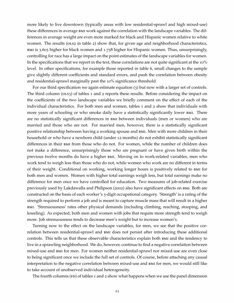
similar neighborhoods so there is very little time series variation from which to estimate the effectof neighborhoods. Second, it may take time before neighborhood affects weight. Third, movingmay be associated with life-cycle events that make it hard to identify an effect on bmi. Table 3

presents three sets of regressions (for men and women) that address these concerns.To address the first concern that moves tend to be between similar neighborhoods so that there

is little time series variation in neighborhood characteristics, we consider a subsample consistingonly of movers who experience large changes in neighborhood characteristics. Specifically, we firstcalculate the magnitude of the change in our residential-sprawl index that would be required tomove an individual from the top of the bottom third of the sample, to the bottom of the top thirdof the sample. We define this magnitude to be a ‘large’ change in the residential-sprawl index. Weproceed similarly for mixed-use. We then restrict attention to movers who experience at least thislarge a change in their neighborhood residential-sprawl index or their neighborhood mixed-useindex over the course of the sample. Column r1 in table 3 shows that even when we restrict thesample to individuals who experience large moves, we cannot detect any effect of neighborhoodon bmi after controlling for unobserved individual effects. We conclude that a lack of time seriesvariation in neighborhood characteristics for individuals does not explain our results.

Next, we consider the possibility that it takes several years for changes in neighborhood toaffect weight. To do this, we construct long differences for a sample of individuals who onlymove once during the study period. Specifically, we restrict the sample of movers to individualswho only move once and only move in either 1990 or 1992. The dependent variable is now the‘long difference’ of bmi. That is, the change in bmi between the first and last year for whichwe observe data for each individual mover. Changes in individual characteristics are calculatedsimilarly.22 As these individuals move in either 1990 or 1992 this gives us between two and fouryears to observe the effect of neighborhood for those individuals. Specification r2 in table 3 showsthat even if we allow longer for changes in neighborhood to affect weight we cannot detect anyeffect of residential-sprawl on bmi after controlling for unobserved individual effects. In fact, formen, higher mixed-use is associated with a statistically significant increase in bmi when we allowmore time for neighborhood to have an effect on weight. This is the only case in which we finda statistically significant coefficient on one of the neighborhood variables in our first-differencespecifications and it runs contrary to what the literature has claimed so far: men in this particularsub-sample who move to a neighborhood with more shops and churches tend to see their weightincrease.

Finally, we consider whether major lifestyle changes that occur at the same time as both movesand changes in unobservable characteristics prevent us from correctly estimating the effect ofneighborhood. To illustrate this problem, consider a hypothetical example where marriage causesevery man to move to a more sprawling neighborhood and this change in neighborhood causes aone pound weight gain. However, marriage also causes a change in unobserved habits which leads

22For most movers, this involves differencing over the whole study period. For a small number of individuals withmissing data, we difference over smaller time periods. The set of time dummies is constructed to allow for the fact thatdifferencing may be over slightly different time periods.

13

Table 3: bmi on residential-sprawl, mixed-use and individual characteristics (sub-samples)Men Women

Variable [r1] [r2] [r3] [r1] [r2] [r3]

Residential-sprawl -0.044 0.186 0.171 -0.114 -0.284 -0.191(0.135) (0.382) (0.217) (0.146) (0.414) (0.236)

Mixed-use 0.567 2.970 0.866 -0.424 -0.175 -0.263(0.687) (1.643)∗ (0.922) (0.632) (1.533) (0.809)

Age 0.538 0.726 0.572 0.487 -1.159 0.368(0.192)∗∗∗ (0.571) (0.250)∗∗ (0.232)∗∗ (0.669)∗ (0.294)

Age2 -0.004 -0.006 -0.006 -0.004 -0.004 -0.003(0.003) (0.003)∗∗ (0.004)∗ (0.003) (0.003) (0.004)

Years schooling 0.122 -0.098 0.102 0.040 0.145 0.107(0.066)∗ (0.132) (0.080) (0.068) (0.109) (0.082)

Daily smoker -0.216 -0.877 0.133 -0.188 -0.530 -0.272(0.244) (0.438)∗∗ (0.253) (0.270) (0.488) (0.403)

Married 0.261 0.308 0.448 0.575(0.080)∗∗∗ (0.233) (0.121)∗∗∗ (0.324)∗

Working spouse 0.017 -0.204 -0.196 0.077 -0.127 -0.047(0.047) (0.192) (0.088)∗∗ (0.084) (0.286) (0.126)

Children in household -0.030 -0.183 0.070 0.060(0.046) (0.091)∗∗ (0.073) (0.117)

Newborn 0.052 0.036 0.544 0.778(0.060) (0.193) (0.081)∗∗∗ (0.205)∗∗∗

Pregnant 1.806 1.782(0.120)∗∗∗ (0.360)∗∗∗

In work -0.192 -0.183 -0.138 -0.143 -0.278 -0.053(0.063)∗∗∗ (0.255) (0.077)∗ (0.066)∗∗ (0.171) (0.088)

Annual hours worked (1,000) -0.050 -0.135 -0.030 -0.037 0.116 -0.070(0.037) (0.094) (0.053) (0.039) (0.104) (0.053)

Annual earnings ($1,000) 0.000 0.002 -0.001 -0.003 -0.011 -0.008(0.002) (0.005) (0.002) (0.002) (0.009) (0.003)∗∗

Job strength -0.560 0.912 0.593 -0.333 0.063 -0.625(0.365) (0.563) (0.470) (0.380) (0.503) (0.477)

Strenuous 0.372 -0.960 -0.595 0.235 -0.442 0.442(0.349) (0.549)∗ (0.481) (0.384) (0.510) (0.529)

Observations 7033 742 3883 7434 1029 3806Individuals 1713 742 945 1774 1029 919R2 0.05 0.34 0.05 0.11 0.28 0.05

Notes: The dependent variable is bmi. Regression results in first differences for restricted sub-samples. r1 restricts thesample of movers to individuals who experience large changes in their neighborhood characteristics. r2 restricts thesample of movers to individuals who only move once and in either 1990 or 1992 and uses long-differences. r3 restrictsthe sample of movers to individuals who do not experience a change in marital status or child-related variables. Wecontinue to use the full set of non-movers to help identify the coefficients on individual characteristics. Year dummiesare included in all specifications. Numbers in parenthesis report clustered standard errors. ∗∗∗, ∗∗, and ∗ indicatesignificance at the 1%, 5% and 10% level, respectively.

14

to a one pound weight loss. In this case, a first difference estimate will fail to correctly estimate thecausal relationship between sprawl and landscape.

To check whether our findings results from these sorts of correlations, we identify two majorlifestyle changes, getting married and starting a family, and exclude all movers who experiencesuch lifestyle changes during the study period.23 We also exclude women who become pregnant.Once again, results reported in column r3 of table 3 show no effect of residential-sprawl or mixed-use for men or women.

To summarize, focusing only on large moves, allowing for a time delay for the effects to occurand looking only at individuals who experience no major life cycle changes does not change ourconclusion that there is no causal relationship between neighborhood and bmi.

We briefly consider three further concerns, not specific to our methodology. The first is that therelationship between the landscape variables and bmi may be non-linear. We find that parametricspecifications including a quadratic term and semi-parametric specifications allowing for arbitrarynon-linearity both show no evidence of a non-linear relationship between bmi and landscape char-acteristics. This concern is closely related to the possibility that people respond in a qualitativelydifferent way to urban and rural landscapes. In preliminary stages of this project we experimentedwith restricting attention to individuals who lived with metropolitan statistical areas. We foundthat this restriction had no qualitative impact on our analysis.

The second concern is that, relative to a number of existing studies, we have not only changedthe method of estimation to control for unobserved propensity to be obese, but also the scale andthe definition of the neighborhood variables. To address this concern, we bring our analysis asclose as possible to that of Ewing et al. (2003), while maintaining our method of estimation. First,we re-estimate our specifications at the county level (the scale of the Ewing et al., 2003, analysis).Our results (not reported) remain qualitatively unchanged for all the specifications reported intables 1 and 2. We then go one step further by re-estimating our specifications at the county leveland measuring sprawl using the same Smart Growth America index as Ewing et al. (2003). Results(reported in Appendix B) show that we still reach the same conclusions about the effect of sprawlon bmi: there is no evidence of a causal relationship between neighborhood and weight. That is,the crucial difference that drives our findings is that we control for unobserved propensity to beobese when estimating the effect of neighborhood on bmi.

A final concern relates to the possibility that our first-difference specification may only capturethe “effect of treatment on the treated” (Heckman and Robb, 1985). This will not matter if the effectof sprawl is the same for all individuals (homogenous treatment effects) but will be a problem ifthe effect of sprawl differs across individuals (heterogeneous treatment effects).24 That is, supposesome people gain weight when they move to a more sprawling neighborhood and others do not.If those who would experience an effect on their weight avoid moving because they do not wish tobecome obese, we will not observe that people who move to more sprawling neighborhoods gainweight even if for some (those that do not move) there would be an effect. However, an advantage

23Specifically, we drop individuals who change marital status or who experience a change in the number of childrenin the household.

24See Heckman, Urzua, and Vytlacil (2006) for a full discussion of the issues concerning heterogenous treatmenteffects.

15

of the issue we are studying is that we observe people moving to less sprawling neighborhoods aswell as to more sprawling neighborhoods. Thus, the flip-side of the above argument is that, justas those who would experience a large effect on their weight from a neighborhood change willtend to self-select out of the more sprawling neighborhood “treatment” (biasing the coefficientsdownwards), they will tend to self-select into the less sprawling neighborhood “treatment” (biasingthe coefficients upwards). If these issues are important, we should see a much smaller effect ofmoves to neighborhoods with higher residential-sprawl and lower mixed-use than of moves toneighborhoods with lower residential-sprawl and higher mixed-use. This is because people whoseweight is particularly affected by neighborhood changes will avoid moves to neighborhoods withhigher residential-sprawl and lower mixed-use that would raise their weight, but will be partic-ularly keen on moves to neighborhoods with lower residential-sprawl and higher mixed-use thatwould lower their weight. In fact, when we allow the effects of increases and decreases in ourneighborhood variables to be different, we find no evidence of statistically significant differences.We conclude that the possibility that people may be more or less likely to move depending on howmoving will affect their weight does not drive our results.

6. Discussion

As discussed above, a number of earlier studies find that people in more sprawling neighborhoodsare heavier than those in less sprawling neighborhoods. These papers use different measures oflandscape.25 They also examine different populations. All find that, however ‘sprawl’ is measuredand whatever the sample used, people in more sprawling neighborhoods are heavier than those inless sprawling neighborhoods. Our results agree with this literature. Whether we measure sprawlwith either of our own two measures of sprawl or with the measure proposed by Ewing et al.

(2003), we find that people living in more sprawling neighborhoods are heavier than those in lesssprawling neighborhoods.

Where we differ from the earlier literature is our focus on, and approach to, determiningwhether people in sprawling neighborhoods are heavier because their neighborhoods caused themto gain weight, or because they were predisposed to be heavy. Our method is simple. We followpeople as they move and check whether changes in neighborhood lead to changes in weight. Iflandscapes cause changes in bmi we should see such a change. We do not.

The obvious criticism of this conclusion is that we fail to discern a causal link between obesityand sprawl because, in one way or another, we do not look hard enough. While we cannot hopeto satisfy every such objection, we can anticipate many of them.

One could think that we fail to find a causal relationship between the residential landscapeand weight because we measure the wrong aspect of landscape. There are three reasons tobelieve that this is not a problem. First, the existing literature and our own results find that thecross-sectional relationship between landscape and weight does not depend sensitively on howlandscape characteristics are measured. Given this, it would be surprising if our longitudinal

25These range from a county based measure based on population density in Ewing et al. (2003), to self-reportedmeasures of landscape in Giles-Corti et al. (2003) and Saelens et al. (2003), to sophisticated gis based measures of parkaccess and street connectivity in Frank et al. (2004).

16

regressions did depend sensitively on the particular measure of landscape. Second, our data setprovides a better combination of scope and detail than existing data sets. Except for the data ofEwing et al. (2003), ours is the only national level data set describing residential landscape. Thisincreases variation in neighborhood characteristics relative to studies focusing on small geographicareas, which should make it easier to find a causal relationship if there was one. Furthermore,relative to the county-level data of Ewing et al. (2003), our data describe neighborhoods at a finerspatial scale and separately identify two key characteristics of neighborhoods that have been linkedto weight gain. Third, when we use counties as geographical units and even when we use thesame measures of sprawl of Ewing et al. (2003) instead of our own, we reach exactly the sameconclusions.

Critics may also object that our sample is too small. We make two points. First, the nlsy hasbeen used extensively to study a wide range of socio-economic phenomena precisely because it is alarge representative sample of the us population born 1958–1965. Not only was it was constructedto be representative, but there has been ‘surprisingly little attrition’ (MaCurdy, Mroz, and Gritz,1998). As we discuss in Appendix A, our main results are not driven by the sample restrictions thatwe then impose to calculate our first difference specification. Second, our sample sizes are largeenough to pick up significant correlations in the cross section. It is differencing out the unobservedpropensity to be obese that makes a difference.

This leads us naturally to the next possible criticism, that our sample does not follow the subjectsfor a long enough period to discern an effect of sprawl on bmi. Here, we start by noting thatfollowing people for just a year is sufficient to pick up the effect of other changes (work status,marriage, and pregnancy). Thus, if sprawl did have an effect it must either be small relative tothese effects, or else, for some reason, occur over a longer time period. To make sure, we haveexplicitly allowed for neighborhood changes to take longer to affect weight. Yet, when we look atthe effect of neighborhood changes over a longer time period, our conclusions are strengthenedrather than weakened.26

Interestingly, two recent studies have taken our suggestion of using movers to identify theeffect of sprawl on obesity, and replicated our methodology using different data. Plantinga andBernell (2007) use the same county-level sprawl measure as Ewing et al. (2003) and, like us, usethe nlsy79.27 They report that individuals in their sample who move to a less sprawling countyexperience a significant weight loss over the subsequent two-year period. Recall that we findno effect of neighborhood changes on weight even when we use the same county-level sprawlmeasure as Ewing et al. (2003), so the difference in results is not due to differences in how wemeasure sprawl. We also find no change when we look at individuals two to four years after theymove, so the difference in results is not due to differences in the time elapsed since the move. Giventhat both our study and theirs use the nlsy79, the difference in results must be due to differences

26See table 3 and the related text for further discussion.27The working paper version of their paper (Plantinga and Bernell, 2005) uses a different methodology. It estimates a

model with two simultaneous equations, one in which weight affects landscape and one in which landscape affectsweight. While the methodology is a priori attractive, identification of their model hinges on the assumption thatmarital status and family size do not affect weight directly, only indirectly through their effect on landscape choice,an assumption that our results show does not hold in the data. The published version (Plantinga and Bernell, 2007)discards those results and adopts our methodology, although with the differences discussed in the text.

17

in the sample of movers. The key is that Plantinga and Bernell study nlsy79 respondents between1996 and 2000, rather than between 1988 and 1994 as we do. This is crucial because at that laterstage in their lives nlsy79 respondents move much less often. Using a county-level sprawl measure(instead of our finer neighborhood definition) and fewer years reduces the number of moves acrossneighborhood types in their sample even further. As a result, Plantinga and Bernell (2007) end upestimating the effect of neighborhood changes on weight on the basis of only 262 movers (less than6% of their sample). This is in contrast to our 4,426 movers (79% of our sample). Furthermoreit appears that their 6% of movers is not representative of the overall population (Plantinga andBernell, 2007, report that their 262 movers are more educated, younger, and more likely to be malethan the general population). It is possible that the disparity between our results and those ofPlantinga and Bernell (2007) reflects the fact the weight of people in their mid to late thirties isvery responsive to sprawl, while the weight of people in their twenties and early thirties is not.However, in light of the discussion above, we are inclined to attribute this disparity to the smalland non-representative sample of movers used for their estimation.

Ewing et al. (2006) is the second paper to adopt our methodology of following movers to attemptto distinguish between sorting and causation. To measure residential landscapes, this paper alsorelies on the county-level sprawl index used in Ewing et al. (2003), although extended to morecounties. The population under study is that of the nlsy97 (not the nlsy79). This survey recordsannually height, weight and demographic information for a sample of approximately 8000 us

adolescents with an average age of about 15 in 1997. They conduct two types of regressions. Thefirst is a cross-sectional analysis which, consistent with the rest of the literature (including ourpaper), finds that individuals who live in more sprawling counties are heavier than those who donot.28 The second type of regression is ‘longitudinal’. While the longitudinal estimator used byEwing et al. (2006) is problematic and has different properties than the first difference estimator thatwe use, it also examines the relationship between changes in bmi and changes in neighborhood.29

Their longitudinal results are nearly identical to those presented here and in the appendix. That is,Ewing et al. (2006) find no effect of sprawl on bmi in their longitudinal estimates.

In sum, there is ample and compelling evidence that, on average, people in more sprawlingneighborhoods are heavier than people in less sprawling neighborhoods. This observation isconsistent with two possible explanations. The first is that sprawl causes people to gain weight.

28Ewing et al. (2006) argue that their cross-sectional results reflect causation rather than sorting because “the choiceof residential location is the parents’ and a youth’s attitudes are not factored into the choice” (Ewing et al., 2006, p465).Even if we accept the proposition that parents ignore their childrens’ preferences when choosing residential locations,parents pass on their genes and many of their attitudes to their children. Since their genes and attitudes also determinethe parents’ neighborhood choices, this will in itself create a relationship between a youth’s attitudes and their parents’neighborhood choice. Therefore, the fact that survey respondents are young does not allow us to disentangle sortingfrom causation in the cross-section. This is confirmed by their longitudinal results, where the relationship betweensprawl and weight vanishes.

29Ewing et al. (2006) use a ‘random effects’ estimator. Unlike the superficially similar first-difference and fixed-effectestimators, random effects estimators produce unbiased estimates only in the event that their is no correlation betweenthe error term and explanatory variables. Since residential landscape is known to be correlated to this error (as shownby our results or those of Plantinga and Bernell, 2007), this assumption is almost certainly violated for the data thatEwing et al. use. In addition, only about half of the nlsy97 respondents move during their study period. Since thesemovers may be systematically different from non-movers in unobservables, their estimates may be subject to selectionbias.

18

The second is that people who are already heavy or who are predisposed to gain weight move tomore sprawling neighborhoods. A natural way to distinguish between these two explanations is tostudy whether a given individual experiences changes in weight when they change neighborhood.Studying a large representative sample of movers, we find no relationship between changes inweight and changes in neighborhood characteristics for a given person, whether we use ourdetailed measures of sprawl or coarser county-level measures, and whether we look at individualsshortly after they move or several years later. We conclude that there is no evidence to support theclaim that sprawl causes obesity, and strong evidence to support the claim that people predisposedto obesity self-select into sprawling neighborhoods.

7. Conclusion

It has been widely observed that urban sprawl is associated with higher rates of obesity. Thisobservation has led many researchers to infer that urban sprawl causes obesity. This evidence doesnot permit this conclusion. The higher observed rates of obesity associated with urban sprawl arealso consistent with the sorting of obese people into sprawling neighborhoods.

In this paper we conduct an analysis which permits us to distinguish between these two possib-ilities. Our results strongly suggest that urban sprawl does not cause weight gain. Rather, peoplewho are more likely to be obese (e.g., because they do not like to walk) are also more likely to moveto sprawling neighborhoods (e.g., because they can more easily move around by car). Of coursethe built environment may still place constraints on the type of exercise that people are able to takeor the nature of the diet that they consume. The key point is that individuals who have a lowerpropensity to being obese will choose to avoid those kinds of neighborhoods. Overall, we find noevidence that neighborhood characteristics have any causal effect on weight.

We recognize that the debate over urban sprawl and obesity is ideologically charged, and thatby contradicting the received literature on sprawl and obesity our conclusions will be controversialand (in some circles) unpopular. However, while our findings contradict the received literatureon sprawl and obesity, they are broadly consistent with other research on neighborhood effectsand the importance of sorting. For example, Combes, Duranton, and Gobillon (2004) find thatmuch of the cross-sectional differences in wage rates across cities may be attributed to the sortingof high and low wage individuals rather than to intrinsic city level differences in productivity.Similarly, Bayer, Ferreira, and McMillan (2007) argue that heterogeneous sorting on the basis ofschool quality and race induces correlations among observed and unobserved neighborhood at-tributes. Durlauf’s (2004) recent survey includes further examples and discussion of the difficultiesthat sorting presents for the empirical literature that considers the effects of neighborhood onsocioeconomic outcomes. Thus, our results are consistent with other findings that sorting ratherthan causation is the mechanism which drives observed differences in individual characteristicsacross places.

It follows immediately from our results that recent calls to redesign cities in order to combat therise in obesity are misguided. Our results do not provide a basis for thinking that such redesigns

19

will have the desired effect, and therefore suggest that resources devoted to this cause will bewasted. The public health battle against obesity is better fought on other fronts.

References

Anderson, Patricia M., Kristin F. Butcher, and Phillip B. Levine. 2003. Maternal employment andoverweight children. Journal of Health Economics 22(3):477–504.

Bayer, Patrick, Fernando Ferreira, and Robert McMillan. 2007. A unified framework for measuringpreferences for schools and neighborhoods. Journal of Political Economy 115(4):588–638.

Burchfield, Marcy, Henry G. Overman, Diego Puga, and Matthew A. Turner. 2006. Causes ofsprawl: A portrait from space. Quarterly Journal of Economics 121(2):587–633.

Cawley, John. 2004. The impact of obesity on wages. Journal of Human Resources 39(2):451–474.

Chou, Shin-Yi, Michael Grossman, and Henry Saffer. 2004. An economic analysis of adultobesity: results from the Behavioral Risk Factor Surveillance System. Journal of Health Economics23(3):565–587.

Combes, Pierre-Philippe, Gilles Duranton, and Laurent Gobillon. 2004. Spatial wage disparities:Sorting matters! Discussion Paper 4240, Centre for Economic Policy Research.

Cutler, David M., Edward L. Glaeser, and Jesse M. Shapiro. 2003. Why have Americans becomemore obese? Journal of Economic Perspectives 17(3):93–118.

Durlauf, Steven N. 2004. Neighborhood effects. In Vernon Henderson and Jacques-François Thisse(eds.) Handbook of Regional and Urban Economics, volume 4. Amsterdam: North-Holland, 2173–2242.

Ewing, Reid, Ross Brownson, and David Berrigan. 2006. Relationship between urban sprawl andweight of United States youth. American Journal of Preventitive Medicine 31(6):464–474.

Ewing, Reid, Rolf Pendall, and Don Chen. 2002. Measuring Sprawl and its Impact. Washington, dc:Smart Growth America.

Ewing, Reid, Tom Schmid, Richard Killingsworth, Amy Zlot, and Stephen Raudenbush. 2003.Relationship between urban sprawl and physical activity, obesity, and morbidity. AmericanJournal of Health Promotion 18(1):47–57.

Ezzati, Majid, Hilarie Martin, Suzanne Skjold, Stephen Vander Hoorn, and Christopher J. L. Mur-ray. 2006. Trends in national and state-level obesity in the usa after correction for self-reportbias: analysis of health surveys. Journal of the Royal Society of Medicine 99(5):250–257.

Flegal, Katherine M., Margaret D. Carroll, Cynthia L. Ogden, and Clifford L. Johnson. 2002. Pre-valence and trends in obesity among us adults, 1999–2000. jama-Journal of the American MedicalAssociation 288(14):1723–1727.

Frank, L. D., M. A. Andresen, and T. L. Schmid. 2004. Obesity relationships with communitydesign, physical activity, and time spent in cars. American Journal of Preventive Medicine 27(2):87–96.

20

Gerberding, Julie L. 2003. cdc’s role in promoting healthy lifestyles. Statement by Julie L. Ger-berding, Director, Centers for Disease Control and Prevention, before the Senate Committee onAppropriations, Subcommittee on Labor, hhs, Education and Related Agencies.

Giles-Corti, B., S. Macintyre, J. P. Clarkson, T. Pikora, and R. J. Donovan. 2003. Environmental andlifestyle factors associated with overweight and obesity in Perth, Australia. American Journal ofHealth Promotion 18(1):93–102.

Glaeser, Edward L. and Matthew E. Kahn. 2004. Sprawl and urban growth. In Vernon Hendersonand Jacques-François Thisse (eds.) Handbook of Regional and Urban Economics, volume 4. Amster-dam: North-Holland, 2481–2527.

Heckman, James J. and Richard Robb, Jr. 1985. Alternative methods for estimating the impact ofinterventions. In James J. Heckman and Burton Singer (eds.) Longitudinal Analysis of Labor MarketData. New York, ny: Cambridge University Press, 156–245.

Heckman, James J., Sergio Urzua, and Edward J. Vytlacil. 2006. Understanding instrumentalvariables in models with essential heterogeneity. Review of Economics and Statistics 88(3):389–432.

Lakdawalla, Darius and Tomas Philipson. 2002. The growth of obesity and technological change: Atheoretical and empirical analysis. Working Paper 8946, National Bureau of Economic Research.

Lakdawalla, Darius, Tomas Philipson, and Jay Bhattacharya. 2005. Welfare-enhancing technolo-gical change and the growth of obesity. American Economic Review 95(2):253–257.

MaCurdy, Thomas, Thomas Mroz, and R. Mark Gritz. 1998. An evaluation of the national longit-udinal survey on youth. Journal of Human Resources 33(2):345–436.

McCann, Barbara A. and Reid Ewing. 2003. Measuring the Health Effects of Sprawl: A NationalAnalysis of Physical Activity, Obesity and Chronic Disease. Washington, dc: Smart Growth America.

Mokdad, A. H., M. K. Serdula, W. H. Dietz, B. A. Bowman, J. S. Marks, and J. P. Koplan. 1999.The spread of the obesity epidemic in the United States, 1991–1998. jama-Journal of the AmericanMedical Association 282(16):1519–1522.

Plantinga, Andrew J. and Stephanie Bernell. 2005. The association between urban sprawl andobesity: Is it a two-way street? Processed, Oregon State University.

Plantinga, Andrew J. and Stephanie Bernell. 2007. The association between urban sprawl andobesity: Is it a two-way street? Journal of Regional Science 45(3):473–92.

Saelens, B. E., J. F. Sallis, J. B. Black, and D. Chen. 2003. Neighborhood-based differences in physicalactivity: An environment scale evaluation. American Journal of Public Health 93(9):1552–1558.

Sierra Club. 2000. Sprawl costs us all: How your taxes fuel suburban sprawl. Washington, dc: SierraClub.

Sturm, R. 2002. The effects of obesity, smoking, and drinking on medical problems and costs.Health Affairs 21(2):245–253.

Vogelmann, James E., Stephen M. Howard, Limin Yang, Charles R. Larson, Bruce K. Wylie,and Nick Van Driel. 2001. Completion of the 1990s National Land Cover data set for theconterminous United States from Landsat Thematic Mapper data and ancillary data sources.Photogrammetric Engineering & Remote Sensing 67(6):650–684.

21

Wooldridge, Jeffrey M. 2002. Econometric Analysis of Cross Section and Panel Data. Cambridge, ma:The mit Press.

World Health Organization. 2003. Obesity and overweight. Fact sheet, World Health Organization.http://www.who.int/dietphysicalactivity/media/en/gsfs_obesity.pdf.

World Health Organization. 2004. Global Strategy on Diet, Physical Activity and Health. Geneva:World Health Organization.

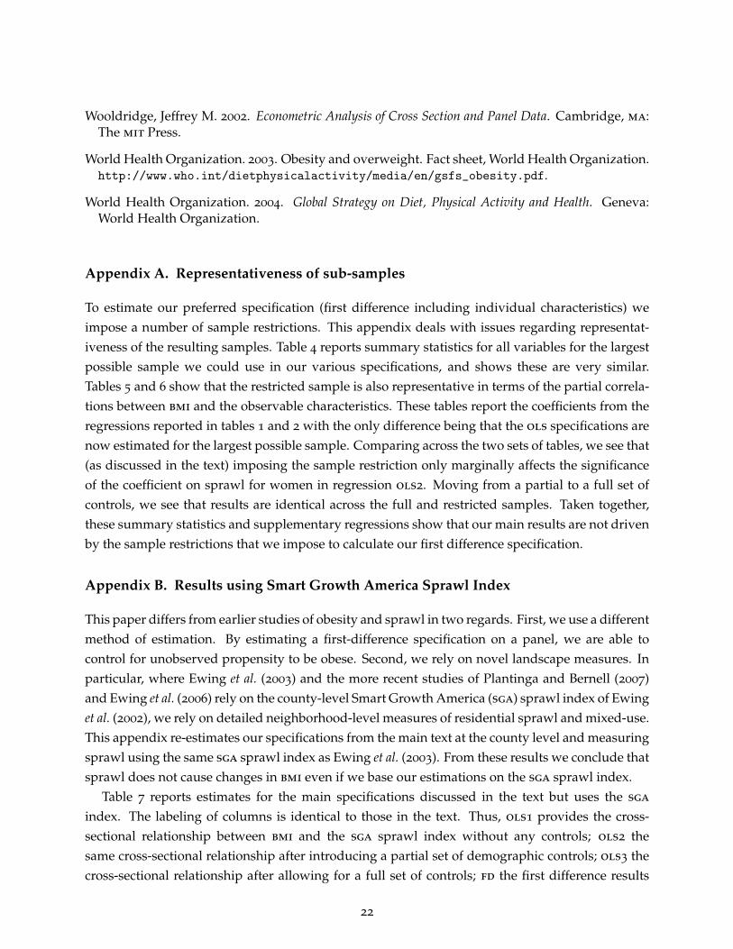
Appendix A. Representativeness of sub-samples

To estimate our preferred specification (first difference including individual characteristics) weimpose a number of sample restrictions. This appendix deals with issues regarding representat-iveness of the resulting samples. Table 4 reports summary statistics for all variables for the largestpossible sample we could use in our various specifications, and shows these are very similar.Tables 5 and 6 show that the restricted sample is also representative in terms of the partial correla-tions between bmi and the observable characteristics. These tables report the coefficients from theregressions reported in tables 1 and 2 with the only difference being that the ols specifications arenow estimated for the largest possible sample. Comparing across the two sets of tables, we see that(as discussed in the text) imposing the sample restriction only marginally affects the significanceof the coefficient on sprawl for women in regression ols2. Moving from a partial to a full set ofcontrols, we see that results are identical across the full and restricted samples. Taken together,these summary statistics and supplementary regressions show that our main results are not drivenby the sample restrictions that we impose to calculate our first difference specification.

Appendix B. Results using Smart Growth America Sprawl Index

This paper differs from earlier studies of obesity and sprawl in two regards. First, we use a differentmethod of estimation. By estimating a first-difference specification on a panel, we are able tocontrol for unobserved propensity to be obese. Second, we rely on novel landscape measures. Inparticular, where Ewing et al. (2003) and the more recent studies of Plantinga and Bernell (2007)and Ewing et al. (2006) rely on the county-level Smart Growth America (sga) sprawl index of Ewinget al. (2002), we rely on detailed neighborhood-level measures of residential sprawl and mixed-use.This appendix re-estimates our specifications from the main text at the county level and measuringsprawl using the same sga sprawl index as Ewing et al. (2003). From these results we conclude thatsprawl does not cause changes in bmi even if we base our estimations on the sga sprawl index.

Table 7 reports estimates for the main specifications discussed in the text but uses the sga

index. The labeling of columns is identical to those in the text. Thus, ols1 provides the cross-sectional relationship between bmi and the sga sprawl index without any controls; ols2 thesame cross-sectional relationship after introducing a partial set of demographic controls; ols3 thecross-sectional relationship after allowing for a full set of controls; fd the first difference results

22

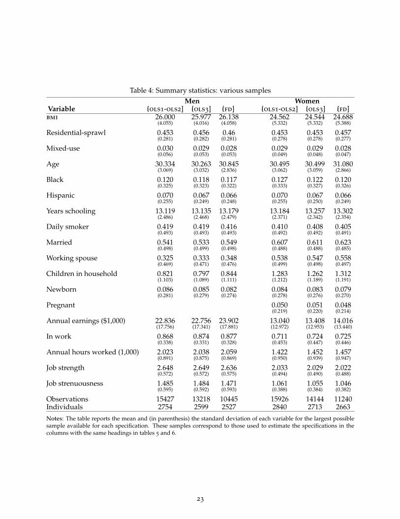
http://www.who.int/dietphysicalactivity/media/en/gsfs_obesity.pdf

Table 4: Summary statistics: various samplesMen Women

Variable [ols1-ols2] [ols3] [fd] [ols1-ols2] [ols3] [fd]bmi 26.000 25.977 26.138 24.562 24.544 24.688

(4.055) (4.016) (4.058) (5.332) (5.332) (5.388)

Residential-sprawl 0.453 0.456 0.46 0.453 0.453 0.457(0.281) (0.282) (0.281) (0.278) (0.278) (0.277)

Mixed-use 0.030 0.029 0.028 0.029 0.029 0.028(0.056) (0.053) (0.053) (0.049) (0.048) (0.047)

Age 30.334 30.263 30.845 30.495 30.499 31.080(3.069) (3.032) (2.836) (3.062) (3.059) (2.866)

Black 0.120 0.118 0.117 0.127 0.122 0.120(0.325) (0.323) (0.322) (0.333) (0.327) (0.326)

Hispanic 0.070 0.067 0.066 0.070 0.067 0.066(0.255) (0.249) (0.248) (0.255) (0.250) (0.249)

Years schooling 13.119 13.135 13.179 13.184 13.257 13.302(2.486) (2.468) (2.479) (2.371) (2.342) (2.354)

Daily smoker 0.419 0.419 0.416 0.410 0.408 0.405(0.493) (0.493) (0.493) (0.492) (0.492) (0.491)

Married 0.541 0.533 0.549 0.607 0.611 0.623(0.498) (0.499) (0.498) (0.488) (0.488) (0.485)

Working spouse 0.325 0.333 0.348 0.538 0.547 0.558(0.469) (0.471) (0.476) (0.499) (0.498) (0.497)

Children in household 0.821 0.797 0.844 1.283 1.262 1.312(1.103) (1.089) (1.111) (1.212) (1.189) (1.191)

Newborn 0.086 0.085 0.082 0.084 0.083 0.079(0.281) (0.279) (0.274) (0.278) (0.276) (0.270)

Pregnant 0.050 0.051 0.048(0.219) (0.220) (0.214)

Annual earnings ($1,000) 22.836 22.756 23.902 13.040 13.408 14.016(17.756) (17.341) (17.881) (12.972) (12.953) (13.440)

In work 0.868 0.874 0.877 0.711 0.724 0.725(0.338) (0.331) (0.328) (0.453) (0.447) (0.446)

Annual hours worked (1,000) 2.023 2.038 2.059 1.422 1.452 1.457(0.891) (0.875) (0.869) (0.950) (0.939) (0.947)

Job strength 2.648 2.649 2.636 2.033 2.029 2.022(0.572) (0.572) (0.575) (0.494) (0.490) (0.488)

Job strenuousness 1.485 1.484 1.471 1.061 1.055 1.046(0.595) (0.592) (0.593) (0.388) (0.384) (0.382)

Observations 15427 13218 10445 15926 14144 11240Individuals 2754 2599 2527 2840 2713 2663

Notes: The table reports the mean and (in parenthesis) the standard deviation of each variable for the largest possiblesample available for each specification. These samples correspond to those used to estimate the specifications in thecolumns with the same headings in tables 5 and 6.

23

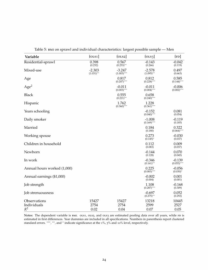
Table 5: bmi on sprawl and individual characteristics: largest possible sample — Men


Residential-sprawl 0.398 0.567 -0.143 -0.042(0.252) (0.253)∗∗ (0.266) (0.119)

Mixed-use -2.303 -3.247 -2.578 0.497(1.031)∗∗ (1.003)∗∗∗ (1.095)∗∗ (0.663)

Age 0.817 0.812 0.585(0.207)∗∗∗ (0.228)∗∗∗ (0.144)∗∗∗

Age2 -0.011 -0.011 -0.006(0.003)∗∗∗ (0.004)∗∗∗ (0.002)∗∗∗

Black 0.555 0.658(0.221)∗∗ (0.240)∗∗∗

Hispanic 1.762 1.228(0.360)∗∗∗ (0.361)∗∗∗

Years schooling -0.152 0.081(0.040)∗∗∗ (0.054)

Daily smoker -1.008 -0.119(0.169)∗∗∗ (0.185)

Married 0.184 0.322(0.180) (0.064)∗∗∗

Working spouse 0.273 -0.030(0.145)∗ (0.037)

Children in household 0.112 0.009(0.083) (0.037)

Newborn -0.144 0.070(0.128) (0.045)

In work -0.346 -0.139(0.161)∗∗ (0.053)∗∗∗

Annual hours worked (1,000) 0.225 -0.056(0.083)∗∗∗ (0.030)∗

Annual earnings ($1,000) -0.002 0.001(0.004) (0.001)

Job strength 1.108 -0.168(0.287)∗∗∗ (0.309)

Job strenuousness -0.697 0.052(0.275)∗∗ (0.292)



24

Table 6: bmi on sprawl and individual characteristics: largest possible sample — Women


Residential-sprawl 0.025 0.578 -0.105 -0.154(0.352) (0.334)∗ (0.345) (0.135)

Mixed-use 0.873 -2.198 -0.731 -0.473(2.180) (1.755) (1.771) (0.640)

Age 0.551 0.815 0.527(0.262)∗∗ (0.287)∗∗∗ (0.186)∗∗∗

Age2 -0.007 -0.011 -0.005(0.004) (0.005)∗∗ (0.003)∗

Black 3.512 2.933(0.323)∗∗∗ (0.355)∗∗∗

Hispanic 1.952 1.326(0.416)∗∗∗ (0.430)∗∗∗

Years schooling -0.254 0.024(0.048)∗∗∗ (0.059)

Daily smoker -0.845 -0.301(0.207)∗∗∗ (0.224)

Married 0.040 0.435(0.298) (0.097)∗∗∗

Working spouse -0.121 0.077(0.238) (0.068)

Children in household -0.019 0.054(0.098) (0.061)

Newborn 0.532 0.592(0.156)∗∗∗ (0.064)∗∗∗

Pregnant 1.833 1.882(0.197)∗∗∗ (0.096)∗∗∗

In work -0.067 -0.170(0.153) (0.053)∗∗∗

Annual hours worked (1,000) 0.370 -0.047(0.097)∗∗∗ (0.032)

Annual earnings ($1,000) -0.030 -0.003(0.008)∗∗∗ (0.002)

Job strength 0.698 -0.491(0.288)∗∗ (0.315)

Job strenuousness 0.757 0.343(0.404)∗ (0.320)



25

that allow for unobserved propensity to be obese; r1 the results when we only consider thesub-sample of movers that experience large changes in neighborhoods; r2 the results when weonly consider the sub-sample of individuals that move once and r3 the results when we onlyconsider the sub-sample of individuals that experience no major life-cycle changes. See the maintext for further discussion of each of these specifications.

Before we discuss our results, note that the sga index is defined such that large numbersrepresent ‘smart’ (i.e. non-sprawling) neighborhoods. Thus, a negative correlation between theindex and bmi implies a positive correlation between sprawl and obesity. Comparing resultswith the relevant specifications from tables 1, 2 and 3 we get essentially identical results. If wecontrol only for age, age2, and race (ols2 specification) we find that men living in more sprawlingneighbourhoods as measured by the sga index tend to have higher bmi. However, once we controlfor individuals’ unobserved propensity to be obese in the fd specification, the coefficient on thesga index is not statistically significant. The robustness checks work as with our neighborhoodvariables — once again, in the first difference regressions only the r2 specification shows a stat-istically significant coefficient on the neighborhood variable, and it runs contrary to the existingliterature: men in this particular sub-sample who move to a neighborhood with less sprawl (highersga index) tend to see their weight increase.30

Overall, we reach the same conclusions regarding the effect of sprawl on bmi if we estimate thesame set of specifications using the sga index of sprawl instead of our two landscape variables.Thus, our conclusions do not depend on our choice of landscape measures, rather they dependsolely on the fact we control for unobserved propensity to be obese when estimating the effect ofneighborhood on bmi. The key point is that, once again, there is no evidence of a causal relationshipbetween neighborhood and weight once we control for unobserved propensity to be obese.

30One potential problem with these estimates, not present in our other results, arises because the sga index iscalculated on the basis of data for 2000, six years after the end of our study period. Thus, we must interpret the sga

measure as a proxy for the equivalent measure calculated for the early 1990s. Since this introduces measurement error, itraises the possibility that our failure to find a relationship between obesity and sprawl in our first difference regressionsusing the sga index is a consequence of attenuation bias. While we are unable to recalculate the sga index for the early1990s, there is reason to think that doing so would not affect our conclusions. The sga index combines various measuresinto a single index, but it mostly captures differences across counties in population density: the correlation betweencounty population density in 2000 and the sga index is about 0.84. Since the correlation between county populationdensity in 1990 and county population density in 2000 is above 0.999, this suggests that a recalculation of the sga indexfor the early 1990s would be very highly correlated with the available index. Thus, it would be surprising if our resultswere sensitive to this change.

26

Table 7: bmi on residential-sprawl, mixed-use and individual characteristics (sub-samples)

Variable [ols1] [ols2] [ols3] [fd] [r1] [r2] [r3]

Mensga index -0.004 -0.006 -0.004 0.001 0.001 0.010 0.001

(0.002) (0.002)∗∗ (0.003) (0.002) (0.002) (0.005)∗ (0.003)

Observations 8915 8915 8103 6281 4271 414 2472Individuals 1684 1684 1684 1684 1157 414 663R2 0.02 0.03 0.07 0.05 0.05 0.35 0.04

Womensga index 0.002 -0.006 -0.003 0.001 0.000 0.001 0.002

(0.004) (0.004) (0.004) (0.002) (0.002) (0.004) (0.002)

Observations 9386 9386 8763 6839 4547 590 2311Individuals 1780 1780 1780 1780 1199 590 611R2 0.01 0.07 0.11 0.12 0.12 0.29 0.04

Notes: The dependent variable is bmi. ols1, ols2, and ols3 are estimated by pooling data over all years. ols1 includesno individual controls. ols2 controls for age, age2, and race. ols3 includes the full set of individual controls. fd, r1, r2,r3 are estimated in first differences. fd uses the full sample of movers and non-movers. r1 restricts the sample of moversto individuals who experience large changes in their neighborhood characteristics. r2 restricts the sample of movers toindividuals who only move once and in either 1990 or 1992 and uses long-differences. r3 restricts the sample of moversto individuals who do not experience a change in marital status or child-related variables. Year dummies are includedin all specifications. Numbers in parenthesis report clustered standard errors. ∗∗∗, ∗∗, and ∗ indicate significance at the1%, 5% and 10% level, respectively.

27

Documents

Fat City: Questioning the Relationship Between Urban