Fast Sweeping Fifth Order WENO Scheme for Static …yzhang10/FS-WENO5.pdf · Fast Sweeping Fifth Order WENO Scheme for Static Hamilton-Jacobi Equations with Accurate Boundary

J Sci Comput (2010) 45: 514–536DOI 10.1007/s10915-010-9345-6

Fast Sweeping Fifth Order WENO Scheme for StaticHamilton-Jacobi Equations with Accurate BoundaryTreatment

Tao Xiong · Mengping Zhang · Yong-Tao Zhang ·Chi-Wang Shu

Received: 7 May 2009 / Revised: 21 December 2009 / Accepted: 23 December 2009 /Published online: 16 January 2010© Springer Science+Business Media, LLC 2010

Abstract A fifth order weighted essentially non-oscillatory (WENO) fast sweeping methodis designed in this paper, extending the result of the third order WENO fast sweeping methodin J. Sci. Comput. 29, 25–56 (2006) and utilizing the two approaches of accurate inflowboundary condition treatment in J. Comput. Math. 26, 1–11 (2008), which allows the usageof Cartesian meshes regardless of the domain boundary shape. The resulting method is testedon a variety of problems to demonstrate its good performance and CPU time efficiency whencompared with lower order fast sweeping methods.

Keywords Fast sweeping method · WENO scheme · Boundary condition

This paper is dedicated to the memory of Professor David Gottlieb.

M. Zhang research supported by NSFC grant 10671190.Y.-T. Zhang research supported by NSF grant DMS-0810413 and Oak Ridge Associated Universities(ORAU) Ralph E. Powe Junior Faculty Enhancement Award.C.-W. Shu research supported by AFOSR grant FA9550-09-1-0126 and NSF grant DMS-0809086.

T. Xiong · M. ZhangDepartment of Mathematics, University of Science and Technology of China, Hefei, Anhui 230026,P.R. China

T. Xionge-mail: [email protected]

M. Zhange-mail: [email protected]

Y.-T. ZhangDepartment of Mathematics, University of Notre Dame, Notre Dame, IN 46556-4618, USAe-mail: [email protected]

C.-W. Shu (�)Division of Applied Mathematics, Brown University, Providence, RI 02912, USAe-mail: [email protected]

mailto:[email protected]




J Sci Comput (2010) 45: 514–536 515

1 Introduction

We are concerned with the numerical solution of the static Hamilton-Jacobi equations{H(φx1 , . . . , φxd

, x) = f (x), x ∈ � \ �

φ(x) = g(x), x ∈ � ⊂ �(1)

where � is a computational domain in Rd with suitable boundary conditions set on thesubset �. The Hamiltonian H is a nonlinear Lipschitz continuous function. Among theHamilton-Jacobi equations, a very important member is the Eikonal equation, which can bedescribed as {

|∇φ(x)| = f (x), x ∈ � \ �

φ(x) = g(x), x ∈ � ⊂ �(2)

where f (x) is a positive function.The static Hamilton-Jacobi equation (1) can be considered as the steady state solution of

the time dependent Hamilton-Jacobi equation

φt + H(φx1 , . . . , φxd, x) = f (x). (3)

The Hamilton-Jacobi equations have abundant applications, such as in optimal control, im-age processing, computer vision, geometric optics, and pedestrian flow models, see, e.g. [2].The solution to (3) or (1) may not always be differentiable or unique. By mimicking theentropy condition for hyperbolic conservation laws to pick out a physically relevant solu-tion, the concept of viscosity solutions was introduced so that a global, physically relevantsolution can be defined for such nonlinear equations which is unique, Lipschitz continuous,but may not be everywhere differentiable.

Numerical discretization for (3) includes first order monotone schemes on structuredmeshes [5] and on unstructured meshes [1], high order essentially non-oscillatory (ENO)schemes on structured meshes [11, 12], high order weighted ENO (WENO) schemes onstructured meshes [9], high order WENO schemes on unstructured meshes [18], and highorder discontinuous Galerkin methods on unstructured meshes [4, 6], among many others.A review of the discretization techniques for the Hamilton-Jacobi equations can be foundin [15]. The difference among these schemes is usually in their spatial discretization. Fora truly time dependent solution, an explicit time discretization, such as the total variationdiminishing (TVD) time discretization in [16], is often used. Such discretization can also beused to obtain the solution of (1) from the steady state solution of (3), marching in time untilthe difference of the numerical solution between successive time steps becomes negligiblysmall. This however may not be the most efficient approach to obtain the solution of (1). Inrecent years, the fast sweeping method has been developed as one of the efficient techniquesfor obtaining the steady state solution of (1). The original fast sweeping method [3, 20] isonly for first order monotone schemes on structured meshes. Later, the fast sweeping methodhas been generalized to some of the high order spatial discretizations. For example, in [19],the fast sweeping method is generalized to the third order WENO scheme of [9]; in [14], itis generalized to fifth order weighted power ENO scheme and a new stopping criterion isproposed; and in [10], it is generalized to the high order discontinuous Galerkin method of[4]. These high order fast sweeping methods are also used in the pedestrian flow simulationsin [8, 17], which require repeated solution of a static Eikonal equation.

516 J Sci Comput (2010) 45: 514–536

The high order fast sweeping methods produce much more accurate solutions on coarsermeshes when compared with the first order fast sweeping method. However, the local solvermight involve more information in the downwind part, and hence the number of iterationsfor convergence to the steady state solution might be significantly larger than that of thefirst order method, and this number might increase when the mesh size is decreased. It istherefore necessary to look carefully at the efficiency of such high order fast sweeping meth-ods, in order to demonstrate their relative CPU time efficiency to first order fast sweepingmethods for achieving the same level of error. Another complication is that the high orderspatial discretization involves a wider stencil and hence the additional difficulty in treatingthe numerical boundary conditions. In [19] and also several other papers on similar meth-ods [8, 10, 17], the values of the numerical solution at these boundary points are eitherfixed with the exact solution, which is not always feasible, or computed with a first orderdiscretization, which would reduce the global accuracy. In [7], two strategies to handle in-flow numerical boundary conditions and solving the static Eikonal equation (2) by usingthe fast sweeping third order WENO scheme in [19] are developed. The first approach usesa first order fast sweeping method to produce numerical solutions with several differentmesh sizes near the boundary, and then forms a Richardson extrapolation to obtain suitablehigh order solution values at the grid points near the inflow boundary. This approach usu-ally involves only a small additional computational cost because the numerical solution atthe grid points near the inflow boundary can often be obtained with only local sweepingin the first order fast sweeping method. The second approach uses a Lax-Wendroff typeprocedure repeatedly utilizing the PDE to write the normal spatial derivatives to the in-flow boundary in terms of the tangential derivatives, which would then be readily availableby the physical inflow boundary condition. With these normal spatial derivatives, we canthen obtain high order solution values at the grid points near the inflow boundary. This ap-proach, when applicable, involves a negligibly small additional computational cost. Thisapproach also allows the usage of Cartesian meshes regardless of the domain boundaryshape, since the boundary does not have to be on grid points. Numerical examples in [7],for the Eikonal equation (2), prove the effectiveness of these boundary conditions treat-ments.

In this paper, we extend the work in [19] of the third order fast sweeping WENO methodto fifth order accuracy, using the classical WENO spatial discretization in [9]. Specialattention is paid to the treatment of numerical boundary conditions, which turns out tobe crucial in guaranteeing accuracy and small number of iterations for convergence. Forinflow boundary conditions, we adopt the two strategies introduced in [7]. For outflowboundary conditions, we apply extrapolation but carefully tune the order of this extrapo-lation so that the number of iterations remains small and the order of accuracy achievedinside the computational domain remains fifth order. We carry out an extensive list ofnumerical experiments and compare the CPU efficiency against lower order fast sweep-ing methods to achieve comparable errors. It is shown that our fast sweeping fifth or-der WENO method converges in a relatively small number of iterations and is more effi-cient in CPU time to achieve the desired error level than lower order fast sweeping meth-ods.

The rest of the paper is organized as follows. The fast sweeping fifth order WENOmethod and the boundary condition treatments are described in Sect. 2. In Sect. 3 we pro-vide several numerical examples to demonstrate the effectiveness and efficiency of the fifthorder fast sweeping method. Concluding remarks are given in Sect. 4.

J Sci Comput (2010) 45: 514–536 517

2 The Fast Sweeping Fifth Order WENO Method and the Treatment of BoundaryConditions

In this section we first give a brief description of the fast sweeping fifth order WENOscheme, following [19]. We then describe the two approaches for the numerical boundaryconditions with fifth order accuracy.

2.1 The Fast Sweeping Fifth Order WENO Scheme

We give a brief description of the fast sweeping fifth order WENO scheme, following [19],for solving the static Hamilton-Jacobi equation (1). For more details, we refer to [9, 19].

For simplicity, we assume that the computational domain � is covered by a tensor prod-uct mesh �h = {(xi, yj ) : 0 ≤ i ≤ I,0 ≤ j ≤ J } and �h = � ∩ �h. We assume without lossof generality that the mesh is uniform, xi = i�x, yj = j�y and �x = �y = h. The approx-imation of the solution to the static Hamilton-Jacobi equation (1) at the location (xi, yj )

is denoted by φi,j , which is obtained by a fast sweeping iterative procedure. As in [7], wedivide the set of mesh points (xi, yj ) into the following four categories:

• Category I contains the points at the inflow part of the domain boundary. The numericalsolution φi,j in Category I is fixed at the prescribed physical boundary condition and doesnot change during the fast sweeping iteration.

• Category II contains the points at the outflow part of the domain boundary, where no phys-ical boundary condition is given, and the ghost points outside the computational domainnear the outflow boundary which are necessary for the wide stencil WENO interpola-tion. The numerical solution φi,j in Category II is obtained by extrapolation of suitableaccuracy, based on the numerical solution inside the computational domain.

• Category III contains the few points inside the computational domain and near the inflowboundary. These points cannot be updated by the WENO scheme because of its widestencil. For the fifth order WENO scheme, any point which has a horizontal or verticaldistance less than 4h from the inflow boundary belongs to this category.

• Category IV contains all the remaining points, which are updated during the fast sweepingiterations until convergence.

The Gauss-Seidel iterations with four alternating direction sweepings are then performedas follows:

(1) i = 0 : I, j = 0 : J ; (2) i = I : 0, j = 0 : J ;(3) i = I : 0, j = J : 0; (4) i = 0 : I, j = J : 0.

(4)

To compute the viscosity solution for (1) in 2D, we discretize the Hamiltonian H by amonotone numerical Hamiltonian H [5]:{

H (φ−x , φ+

x ;φ−y , φ+

y )ij = f (xi, yj ), (i, j) ∈ �h \ �h

φij = gij , (i, j) ∈ �h ⊂ �h.(5)

There are at least two types of numerical Hamiltonian that we can use to solve the non-linear problem. The first is the Godunov type numerical Hamiltonian, which can be usedfor the Eikonal equation (2) as well as the general Hamilton-Jacobi equations (1) withH(u,v) = η(u2, v2) where η is a monotone function with respect to both arguments (see[15]). The second type of monotone numerical Hamiltonian, suitable for discretizing a gen-eral Hamiltonian H(u,v), is the Lax-Friedrichs numerical Hamiltonian which is the sim-plest among all monotone numerical Hamiltonians.

518 J Sci Comput (2010) 45: 514–536

2.1.1 Godunov Type Hamiltonian

For the Eikonal equation (2), the local solution procedure for the fifth order WENO schemeto update the new solution at the grid (i, j) is as follows:

φnewi,j =

⎧⎨⎩

min(φx mini,j , φ

y mini,j ) + fi,j h, if |φx min

i,j − φy mini,j | ≥ fi,jh,

φx mini,j

+φy mini,j

+(2f 2i,j

h2−(φx mini,j

−φy mini,j

)2)12

2 , otherwise(6)

where fi,j = f (xi, yj ), and{φx min

i,j = min(φi,j − h(φx)

−i,j , φi,j + h(φx)

+i,j

)φ

y mini,j = min

(φi,j − h(φy)

−i,j , φi,j + h(φy)

+i,j

) (7)

with

(φx)−i,j = ω0(φx)

−,0i,j + ω1(φx)

−,1i,j + ω2(φx)

−,2i,j (8)

where

ω0 + ω1 + ω2 = 1 (9)

and

(φx)−,0i,j = 1

3

�+x φi−3,j

h− 7

6

�+x φi−2,j

h+ 11

6

�+x φi−1,j

h

(φx)−,1i,j = −1

6

�+x φi−2,j

h+ 5

6

�+x φi−1,j

h+ 1

3

�+x φi,j

h(10)

(φx)−,2i,j = 1

3

�+x φi−1,j

h+ 5

6

�+x φi,j

h− 1

6

�+x φi+1,j

h

in which

�+x φi,j = φi+1,j − φi,j , �−

x φi,j = φi,j − φi−1,j .

Similarly, we can define (φx)+i,j . The nonlinear weights are defined by (9) and

ω0 = α0

α0 + α1 + α2, ω2 = α2

α0 + α1 + α2

with

α0 = 1

(ε + IS0)2, α1 = 6

(ε + IS1)2, α2 = 3

(ε + IS2)2

and

IS0 = 13(a − b)2 + 3(a − 3b)2

IS1 = 13(b − c)2 + 3(b + c)2

IS2 = 13(c − d)2 + 3(3c − d)2

where

a = �−x �+

x φi−2,j

h, b = �−

x �+x φi−1,j

h, c = �−

x �+x φi,j

h, d = �−

x �+x φi+1,j

h.

J Sci Comput (2010) 45: 514–536 519

The definitions for (φy)−i,j and (φy)

+i,j are analogous. Here ε is a small number in the WENO

nonlinear weights. In the description above, φnewi,j denotes the to-be-updated numerical solu-

tion for φ at the grid point (i, j), and φi,j denotes the currently available value of φ.Convergence is declared if ∥∥φnew − φold

∥∥ ≤ δ, (11)

where δ is a given convergence threshold value and φoldi,j denotes the old value of φ before

the start of the current sweeping step. L1 norm is used in (11).

2.1.2 Lax-Friedrichs Type Hamiltonian

We define

H LF (u−, u+;v−, v+) = H

(u− + u+

2,v− + v+

2

)− 1

2αx(u

+ − u−) − 1

2αy(v

+ − v−)

where

αx = maxA≤u≤BC≤v≤D

|H1(u, v)|, αy = maxA≤u≤BC≤v≤D

|H2(u, v)|. (12)

Here Hi(u, v) is the partial derivative of H with respect to the ith argument, or the Lipschitzconstant of H with respect to the ith argument. [A,B] is the value range for u±, and [C,D]is the value range for v±. The Lax-Friedrichs numerical Hamiltonian is monotone whenA ≤ u ≤ B , C ≤ v ≤ D. The high order Lax-Friedrichs fast sweeping scheme for staticHamilton-Jacobi equations can be written as:

φnewi,j =

(h

αx + αy

)[f − H

((φx)

−i,j + (φx)

+i,j

2,(φy)

−i,j + (φy)

+i,j

2

)

+ αx

(φx)+i,j − (φx)

−i,j

2+ αy

(φy)+i,j − (φy)

−i,j

2

]+ φold

i,j (13)

where φi,j denotes the currently available value of φ.

2.1.3 Initial Quess

For high order Godunov type numerical Hamiltonian, the solution from the first-order Go-dunov fast sweeping method [20] is used as the initial guess for all the grid points in Cat-egory IV. Grid values in Categories I and III are fixed as appropriate, and before each it-eration, grid values in Category II are obtained by suitable extrapolation. For high orderLax-Friedrichs numerical Hamiltonian, grid values in Categories I, II and III are assignedthe same as the Godunov type Hamiltonian, and large values (emulating +∞) are used asthe initial guess for all the grid points in Category IV.

2.2 Boundary Treatment

In this subsection we describe briefly the two types of boundary treatments developed in [7],for points in Category III as defined in the previous subsection.

520 J Sci Comput (2010) 45: 514–536

2.2.1 Strategy I: Richardson Extrapolation

This procedure starts with several first order accurate solutions with different mesh sizes,then the Richardson extrapolation is used to obtain high order accurate point values forthose points in Category III. This is feasible without excessive computational cost becausepoints in Category III are close to the inflow boundary, hence the first order fast sweepingiterations can be performed locally, greatly reducing the computational cost.

Assume Ih is the numerical solution of the first order fast sweeping scheme with meshsize h at the location (x∗, y∗), which is a grid point in Category III. If we further assume

Ih − I = β1h + β2h2 + β3h

3 + β4h4 + O(h5)

with constant coefficients βi , where I is the exact solution at the location (x∗, y∗), which isreasonable when the exact solution is smooth enough, then

Ih = 1

315Ih − 2

21Ih/2 + 8

9Ih/4 − 64

21Ih/8 + 1024

315Ih/16 (14)

would be a fifth order approximation to I :

Ih − I = O(h5).

This boundary treatment strategy is suitable for most types of inflow boundaries, includ-ing the source boundary consisting of a single point. The efficiency of this strategy how-ever depends on how fast we can compute the first order approximations Ih, Ih/2, Ih/4, Ih/8

and Ih/16 for all grid points inside Category III. When the characteristics from the inflowboundary do not intersect with each other, such first order fast sweeping computation canbe performed locally and is very fast. When the characteristics from the inflow boundary dointersect with each other, the efficiency of this strategy would decrease. Fortunately, in thiscase the inflow boundary would not be a single point, hence the second strategy describednext would usually be applicable.

2.2.2 Strategy II: The Lax-Wendroff Type Procedure

This procedure is based on Taylor expansions and then on converting normal derivatives bytangential derivatives on the boundary based on repeated usage of the PDE. To fix the ideas,let us assume that the left boundary

� = {(x, y) : x = 0, 0 ≤ y ≤ 1} (15)

of the computational domain [0,1]2 is the inflow boundary, on which the solution is givenas

φ(0, y) = g(y), 0 ≤ y ≤ 1.

We would like to obtain a high order approximation to the solution value φi,j ≈ φ(xi, yj )

for i = 1,2,3 and a fixed j , which corresponds to a point (xi, yj ) in Category III. A simpleTaylor expansion gives, for i = 1,2,3,

φ(xi, yj ) = φ(0, yj ) + ihφx(0, yj ) + (ih)2

2φxx(0, yj ) + (ih)3

3! φxxx(0, yj )

J Sci Comput (2010) 45: 514–536 521

+ (ih)4

4! φxxxx(0, yj ) + O(h5)

hence the fifth order approximation is

φi,j = φ(0, yj ) + ihφx(0, yj ) + (ih)2

2φxx(0, yj ) + (ih)3

3! φxxx(0, yj ) + (ih)4

4! φxxxx(0, yj ).

We already have φ(0, yj ) = g(yj ). The PDE (1), evaluated at the point (0, yj ), becomes

H(φx(0, yj ), g′(yj )) = f (0, yj ) (16)

in which the only unknown quantity is φx(0, yj ). Solving this (usually nonlinear) equationshould give us φx(0, yj ). There might be more than one root, in which case we should choosethe root so that

∂uH(φx(0, yj ), g′(yj )) > 0 (17)

where ∂u refers to the partial derivative with respect to the first argument in H(u,v). Thecondition (17) guarantees that the boundary � in (15) is an inflow boundary. If the condition(17) still cannot pin down a root, then we would choose the root which is closest to the valuefrom the first order fast sweeping solution at the same grid point. To obtain φxx(0, yj ), wefirst take the derivative with respect to y on the original PDE (1), and then evaluate it at thepoint (0, yj ), which yields

∂uH(φx(0, yj ), g′(yj ))φxy(0, yj ) + ∂vH(φx(0, yj ), g

′(yj ))g′′(yj ) = fy(0, yj ), (18)

where ∂u and ∂v refer to the partial derivatives with respect to the first and second argumentsin H(u,v), respectively. In this equation the only unknown quantity is φxy(0, yj ), hence weobtain easily its value, thanks to (17). We then take the derivative with respect to x on theoriginal PDE (1), and evaluate it at the point (0, yj ) to obtain

∂uH(φx(0, yj ), g′(yj ))φxx(0, yj ) + ∂vH(φx(0, yj ), g

′(yj ))φxy(0, yj ) = fx(0, yj ).

This time, the only unknown quantity is φxx(0, yj ), which we can obtain readily fromthis equality. Following the same procedure, we can obtain the values of φxxx(0, yj ) andφxxxx(0, yj ). We remark that this approach allows the usage of Cartesian meshes regardlessof the shape of the domain boundary �, for example, a curved boundary, since the boundarydoes not have to be on grid points. We refer to [7] for more details.

3 Numerical Examples

In this section, we demonstrate the effectiveness and efficiency of the fast sweeping fifthorder WENO method, denoted by “swp5”, with accurate boundary treatment through a fewtwo dimensional (2-D) numerical examples. Results of fast sweeping third order WENOmethod, denoted by “swp3”, and first order fast sweeping method, denoted by “swp1”,are also included in some cases for comparison. The order of extrapolation on the outflowboundary is taken as 3 for the fast sweeping fifth order WENO method. This choice givesa faster convergence of the fast sweeping iterations, and does not affect the designed fifthorder accuracy away from the outflow boundary. When such extrapolation is used, the er-rors are computed in a smaller inner box of length 2h0 away from the outer boundary, where

522 J Sci Comput (2010) 45: 514–536

h0 refers to the coarsest mesh size. In our computation, the small number ε in the nonlin-ear WENO weights is taken to be 10−6, and the threshold value δ at which iteration stopsis taken to be δ = 10−14. Exceptions will be explicitly described in the examples. We listthe number of iterations in our tables, noticing that each iteration contains four sweepings.Except for the last example, the Godunov type numerical Hamiltonian is used.

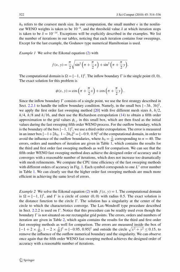
Example 1 We solve the Eikonal equation (2) with

f (x, y) = π

2

√sin2

(π + π

2x)

+ sin2(π + π

2y).

The computational domain is � = [−1,1]2. The inflow boundary � is the single point (0,0).The exact solution for this problem is

φ(x, y) = cos(π + π

2x)

+ cos(π + π

2y)

.

Since the inflow boundary � consists of a single point, we use the first strategy described inSect. 2.2.1 to handle the inflow boundary condition. Namely, in the small box [−3h, 3h]2,we apply the first order fast sweeping method [20] with five different mesh sizes h, h/2,h/4, h/8 and h/16, and then use the Richardson extrapolation (14) to obtain a fifth orderapproximation to the grid values φi,j in this small box, which are then fixed as the initialvalues during the fast sweeping fifth order WENO process. For the outflow boundary, whichis the boundary of the box [−1,1]2, we use a third order extrapolation. The error is measuredin an inner box [−1+2h0, 1−2h0]2 = [−0.9, 0.9]2 of the computational domain, in order toavoid the influence of the outflow boundaries, where h0 = 2

40 corresponding to n = 40. Theerrors, orders and numbers of iteration are given in Table 1, which contains the results forthe third and first order fast sweeping methods as well for comparison. We can see that thefifth order WENO fast sweeping method does achieve the designed order of accuracy and itconverges with a reasonable number of iterations, which does not increase too dramaticallywith mesh refinements. We compare the CPU time efficiency of the fast sweeping methodswith different orders of accuracy in Fig. 1. Each symbol corresponds to one L1 error numberin Table 1. We can clearly see that the higher order fast sweeping methods are much moreefficient in achieving the same level of errors.

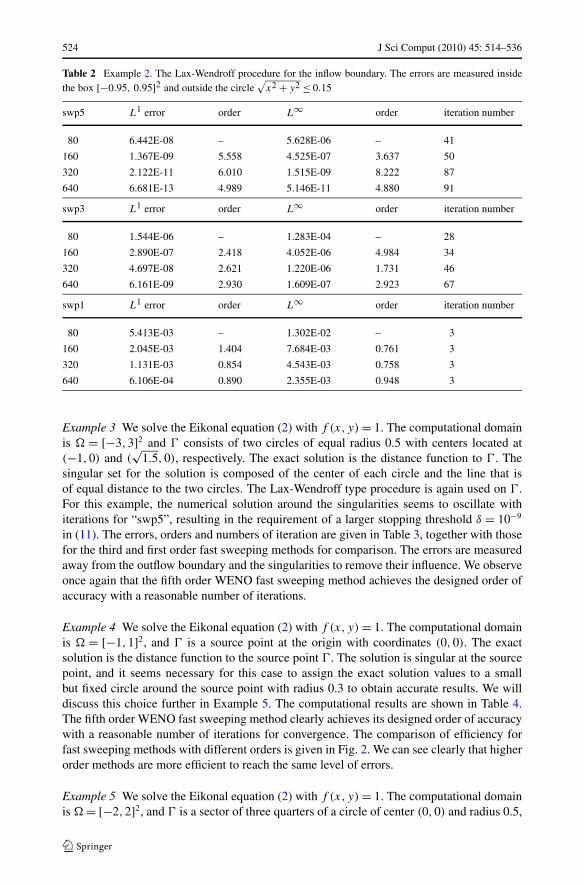
Example 2 We solve the Eikonal equation (2) with f (x, y) = 1. The computational domainis � = [−1,1]2, and � is a circle of center (0,0) with radius 0.5. The exact solution isthe distance function to the circle �. The solution has a singularity at the center of thecircle to which the characteristics converge. The Lax-Wendroff type procedure describedin Sect. 2.2.2 is used on �. Notice that this procedure can be readily used even though theboundary � is not situated on our rectangular grid points. The errors, orders and numbers ofiteration are given in Table 2, which again contains the results for the third and first orderfast sweeping methods as well for comparison. The errors are measured inside the box of[−1 + 2 × 2

80 , 1 − 2 × 280 ]2 = [−0.95, 0.95]2 and outside the circle

√x2 + y2 ≤ 0.15, to

remove the influence of the outflow numerical boundary and the singularity. We can observeonce again that the fifth order WENO fast sweeping method achieves the designed order ofaccuracy with a reasonable number of iterations.

J Sci Comput (2010) 45: 514–536 523

Table 1 Example 1. Richardson procedure for the inflow boundary. The errors are measured in the box of[−0.9,0.9]2

swp5 L1 error order L∞ order iteration number

40 9.308E-06 – 9.837E-05 – 50

80 1.090E-07 6.417 1.601E-06 5.941 53

160 8.973E-10 6.924 2.241E-08 6.158 66

320 2.938E-12 8.255 3.340E-11 9.390 84

640 5.521E-14 5.743 1.374E-13 7.925 117


40 1.451E-04 – 4.931E-04 – 50

80 1.238E-05 3.551 3.099E-05 3.992 36

160 8.281E-07 3.902 1.505E-06 4.364 44

320 9.283E-08 3.157 1.557E-07 3.273 58

640 1.163E-08 2.996 1.933E-08 3.010 90


40 4.735E-02 – 7.671E-02 – 2

80 2.356E-02 1.007 3.857E-02 0.992 2

160 1.175E-02 1.004 1.934E-02 0.996 2

320 5.866E-03 1.002 9.683E-03 0.998 2

640 2.931E-03 1.001 4.845E-03 0.999 2

1280 1.465E-03 1.001 2.423E-03 0.999 2

2560 7.324E-04 1.000 1.212E-03 1.000 2

Fig. 1 Example 1. L1 errorversus CPU time

524 J Sci Comput (2010) 45: 514–536

Table 2 Example 2. The Lax-Wendroff procedure for the inflow boundary. The errors are measured insidethe box [−0.95, 0.95]2 and outside the circle

√x2 + y2 ≤ 0.15


80 6.442E-08 – 5.628E-06 – 41

160 1.367E-09 5.558 4.525E-07 3.637 50

320 2.122E-11 6.010 1.515E-09 8.222 87

640 6.681E-13 4.989 5.146E-11 4.880 91


80 1.544E-06 – 1.283E-04 – 28

160 2.890E-07 2.418 4.052E-06 4.984 34

320 4.697E-08 2.621 1.220E-06 1.731 46

640 6.161E-09 2.930 1.609E-07 2.923 67


80 5.413E-03 – 1.302E-02 – 3

160 2.045E-03 1.404 7.684E-03 0.761 3

320 1.131E-03 0.854 4.543E-03 0.758 3

640 6.106E-04 0.890 2.355E-03 0.948 3

Example 3 We solve the Eikonal equation (2) with f (x, y) = 1. The computational domainis � = [−3,3]2 and � consists of two circles of equal radius 0.5 with centers located at(−1,0) and (

√1.5,0), respectively. The exact solution is the distance function to �. The

singular set for the solution is composed of the center of each circle and the line that isof equal distance to the two circles. The Lax-Wendroff type procedure is again used on �.For this example, the numerical solution around the singularities seems to oscillate withiterations for “swp5”, resulting in the requirement of a larger stopping threshold δ = 10−9

in (11). The errors, orders and numbers of iteration are given in Table 3, together with thosefor the third and first order fast sweeping methods for comparison. The errors are measuredaway from the outflow boundary and the singularities to remove their influence. We observeonce again that the fifth order WENO fast sweeping method achieves the designed order ofaccuracy with a reasonable number of iterations.

Example 4 We solve the Eikonal equation (2) with f (x, y) = 1. The computational domainis � = [−1,1]2, and � is a source point at the origin with coordinates (0,0). The exactsolution is the distance function to the source point �. The solution is singular at the sourcepoint, and it seems necessary for this case to assign the exact solution values to a smallbut fixed circle around the source point with radius 0.3 to obtain accurate results. We willdiscuss this choice further in Example 5. The computational results are shown in Table 4.The fifth order WENO fast sweeping method clearly achieves its designed order of accuracywith a reasonable number of iterations for convergence. The comparison of efficiency forfast sweeping methods with different orders is given in Fig. 2. We can see clearly that higherorder methods are more efficient to reach the same level of errors.

Example 5 We solve the Eikonal equation (2) with f (x, y) = 1. The computational domainis � = [−2,2]2, and � is a sector of three quarters of a circle of center (0,0) and radius 0.5,

J Sci Comput (2010) 45: 514–536 525

Table 3 Example 3. Lax-Wendroff procedure for the inflow boundary. The errors are measured in the box

[−2.85,2.85]2, outside the circles√

(x + 1)2 + y2 ≤ 0.15 and√

(x − √1.5)2 + y2 ≤ 0.15, and outside the

region |x − 0.5(√

1.5 − 1)| ≤ 0.15. δ = 10−9 for “swp5”


80 1.710E-06 – 2.567E-04 – 63

160 1.652E-07 3.372 2.153E-05 3.576 70

320 5.510E-09 4.906 3.523E-06 2.612 55

640 1.090E-10 5.659 5.797E-08 5.925 73


80 1.596E-04 – 2.737E-03 – 43

160 1.007E-05 3.986 7.663E-04 1.837 45

320 6.814E-07 3.886 2.937E-05 4.705 49

640 1.350E-07 2.335 3.362E-06 3.127 70


80 1.596E-02 – 4.263E-02 – 2

160 8.486E-03 0.911 2.213E-02 0.946 2

320 4.287E-03 0.985 1.125E-02 0.976 2

640 2.162E-03 0.987 5.679E-03 0.987 3

closed with the x-axis and y-axis in the first quadrant, which can be described as

� = {(x, y) :√

x2 + y2 = 0.5, if x ≤ 0 or y ≤ 0} ∪ {(x,0) : 0 ≤ x ≤ 0.5}∪ {(0, y) : 0 ≤ y ≤ 0.5}.

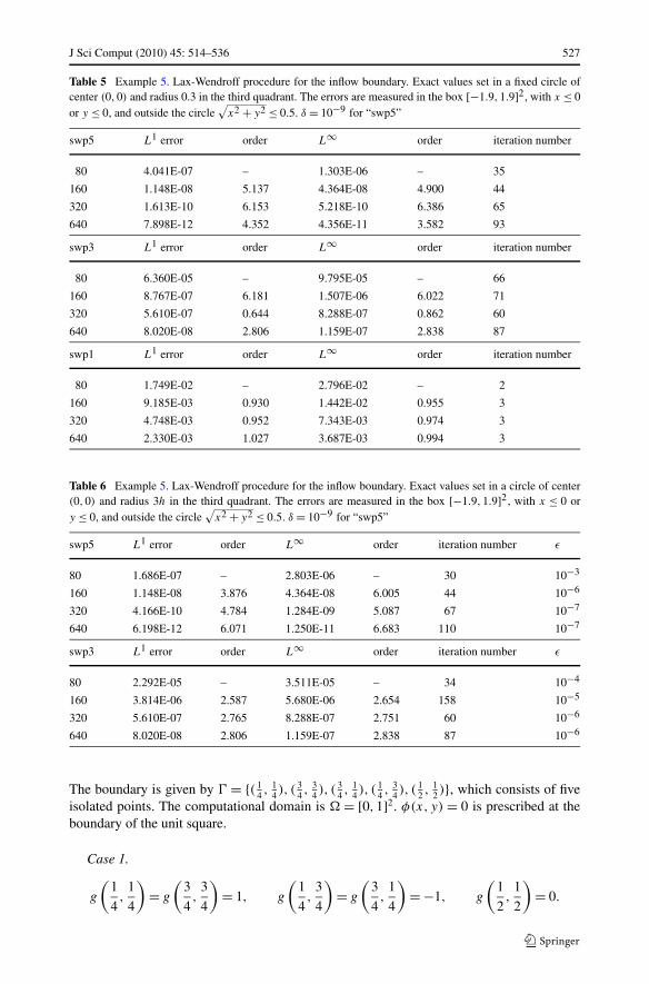
The exact solution is the distance function to the boundary �. Singularities at the two cornersin � give rise to different scenarios in different regions, which include both shocks andrarefaction waves. The Lax-Wendroff type procedure described in Sect. 2.2.2 is used on �,but we set exact values in a fixed circle of center (0,0) and radius 0.3 in the third quadrant asin Example 4. Similar to Example 3, we use a larger threshold δ = 10−9 for “swp5” becauseof the singularities. We list the errors, orders, and numbers of iterations in Table 5, wherethe errors are measured in the smooth region inside the box [−2 + 2 × 4

80 ,2 − 2 × 480 ]2 =

[−1.9,1.9]2, with x ≤ 0 or y ≤ 0, and outside the circle√

x2 + y2 ≤ 0.5. The designed orderof accuracy is clearly achieved and the number of iterations is quite reasonable. For thisexample, if we only assign exact values in a small circle with radius 3h instead of a fixed-sizecircle around the point (0,0), we would need to adjust the size of ε in the WENO weightsto obtain satisfactory results, which are listed in Table 6. The pattern for the choice of ε is touse a larger value for coarser meshes, favoring the underlying linear scheme and reducingthe nonlinear WENO effect to avoid iteration convergence difficulties for coarser meshes.

Example 6 (Shape-from-shading) This and the next examples are about the shape underisolated light sources, see [13] for more details. We solve the Eikonal equation (2) with

f (x, y) = 2π√

[cos(2πx) sin(2πy)]2 + [sin(2πx) cos(2πy)]2. (19)

526 J Sci Comput (2010) 45: 514–536

Table 4 Example 4. The exact solution values are assigned to a small box with length 0.3 around the sourcepoint. The errors are measured in the box [−0.9,0.9]2


40 4.794E-06 – 1.155E-05 – 37

80 1.355E-07 5.145 3.193E-07 5.177 42

160 1.453E-09 6.543 4.458E-09 6.163 54

320 3.689E-11 5.299 9.896E-11 5.493 72

640 1.069E-12 5.109 2.812E-12 5.137 101


40 2.111E-04 – 4.454E-04 – 41

80 3.878E-06 5.766 8.596E-06 5.695 30

160 5.650E-07 2.779 1.362E-06 2.658 38

320 7.949E-08 2.830 1.879E-07 2.858 52

640 9.772E-09 3.024 2.319E-08 3.018 75


40 2.771E-02 – 4.964E-02 – 2

80 1.706E-02 0.700 3.022E-02 0.716 2

160 1.024E-02 0.736 1.794E-02 0.752 2

320 6.020E-03 0.766 1.043E-02 0.782 2

640 3.478E-03 0.792 5.959E-03 0.807 2

1280 1.980E-03 0.813 3.356E-03 0.828 2

2560 1.112E-03 0.832 1.868E-03 0.845 2

Fig. 2 Example 4. L1 errorversus CPU time

J Sci Comput (2010) 45: 514–536 527

Table 5 Example 5. Lax-Wendroff procedure for the inflow boundary. Exact values set in a fixed circle ofcenter (0,0) and radius 0.3 in the third quadrant. The errors are measured in the box [−1.9,1.9]2, with x ≤ 0or y ≤ 0, and outside the circle

√x2 + y2 ≤ 0.5. δ = 10−9 for “swp5”


80 4.041E-07 – 1.303E-06 – 35

160 1.148E-08 5.137 4.364E-08 4.900 44

320 1.613E-10 6.153 5.218E-10 6.386 65

640 7.898E-12 4.352 4.356E-11 3.582 93


80 6.360E-05 – 9.795E-05 – 66

160 8.767E-07 6.181 1.507E-06 6.022 71

320 5.610E-07 0.644 8.288E-07 0.862 60

640 8.020E-08 2.806 1.159E-07 2.838 87


80 1.749E-02 – 2.796E-02 – 2

160 9.185E-03 0.930 1.442E-02 0.955 3

320 4.748E-03 0.952 7.343E-03 0.974 3

640 2.330E-03 1.027 3.687E-03 0.994 3

Table 6 Example 5. Lax-Wendroff procedure for the inflow boundary. Exact values set in a circle of center(0,0) and radius 3h in the third quadrant. The errors are measured in the box [−1.9,1.9]2, with x ≤ 0 ory ≤ 0, and outside the circle

√x2 + y2 ≤ 0.5. δ = 10−9 for “swp5”

swp5 L1 error order L∞ order iteration number ε

80 1.686E-07 – 2.803E-06 – 30 10−3

160 1.148E-08 3.876 4.364E-08 6.005 44 10−6

320 4.166E-10 4.784 1.284E-09 5.087 67 10−7

640 6.198E-12 6.071 1.250E-11 6.683 110 10−7


80 2.292E-05 – 3.511E-05 – 34 10−4

160 3.814E-06 2.587 5.680E-06 2.654 158 10−5

320 5.610E-07 2.765 8.288E-07 2.751 60 10−6

640 8.020E-08 2.806 1.159E-07 2.838 87 10−6

The boundary is given by � = {( 14 , 1

4 ), ( 34 , 3

4 ), ( 34 , 1

4 ), ( 14 , 3

4 ), ( 12 , 1

2 )}, which consists of fiveisolated points. The computational domain is � = [0,1]2. φ(x, y) = 0 is prescribed at theboundary of the unit square.

Case 1.

g

(1

4,

1

4

)= g

(3

4,

3

4

)= 1, g

(1

4,

3

4

)= g

(3

4,

1

4

)= −1, g

(1

2,

1

2

)= 0.

528 J Sci Comput (2010) 45: 514–536

Table 7 Example 6 (Case 1). Exact values set on all grid points of a small box with length of 4h to the pointsof ( 1

2 , 12 ), ( 1

4 , 14 ), ( 1

4 , 34 ), ( 3

4 , 14 ) and ( 3

4 , 34 ) for “swp5” and 2h for “swp3”. The errors are measured on the

whole computational domain


80 4.714E-08 – 1.938E-07 – 39 10−3

160 1.949E-09 4.596 7.188E-09 4.753 52 10−4

320 6.211E-11 4.972 2.199E-10 5.031 72 10−5

640 1.832E-12 5.083 6.394E-12 5.104 109 10−6


80 3.413E-05 – 1.209E-04 – 28 10−4

160 4.682E-06 2.866 1.561E-05 2.953 37 10−5

320 5.989E-07 2.967 1.951E-06 3.000 55 10−6

640 6.979E-08 3.101 2.294E-07 3.088 84 10−6


80 3.177E-02 – 6.040E-02 – 4

160 1.667E-02 0.930 3.052E-02 0.985 4

320 8.573E-03 0.959 1.534E-02 0.992 4

640 4.359E-03 0.976 7.691E-03 0.996 4

The exact solution for this case is

φ(x, y) = sin(2πx) sin(2πy)

which is a smooth function.Case 2.

g

(1

4,

1

4

)= g

(3

4,

3

4

)= g

(1

4,

3

4

)= g

(3

4,

1

4

)= 1, g

(1

2,

1

2

)= 2.

The exact solution to this case is

φ(x, y) =

⎧⎪⎨⎪⎩

max (| sin(2πx) sin(2πy)|,1 + cos(2πx) cos(2πy)) ,

if |x + y − 1| < 12 and |x − y| < 1

2 ;| sin(2πx) sin(2πy)|, otherwise.

This solution is not smooth.For this problem, since � consists of isolated points, the Lax-Wendroff procedure cannot

be applied. Our numerical experiments also indicate that the Richardson procedure does notproduce the desired accuracy for this test case. This could be due to the fact that there aresingular points of the PDE in �. We set the exact solution to a small box with a length of 4h

around the isolated points for Case 1 and 3h for Case 2. The results for these two cases areshown in Tables 7 and 8 respectively. The results seems better for this example if we choosethe parameter ε in the WENO weights depending on the mesh sizes, the choice is listed inthe tables. Again, the pattern for the choice of ε is to use a larger value for coarser meshes.For Case 1 with a smooth solution, we observe the designed fifth order accuracy for the fastsweeping fifth order WENO method, with reasonable number of iterations. For Case 2 with

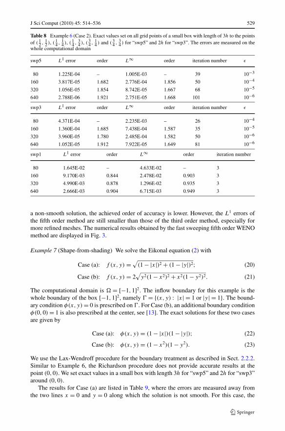
J Sci Comput (2010) 45: 514–536 529

Table 8 Example 6 (Case 2). Exact values set on all grid points of a small box with length of 3h to the pointsof ( 1

2 , 12 ), ( 1

4 , 14 ), ( 1

4 , 34 ), ( 3

4 , 14 ) and ( 3

4 , 34 ) for “swp5” and 2h for “swp3”. The errors are measured on the

whole computational domain


80 1.225E-04 – 1.005E-03 – 39 10−3

160 3.817E-05 1.682 2.776E-04 1.856 50 10−4

320 1.056E-05 1.854 8.742E-05 1.667 68 10−5

640 2.788E-06 1.921 2.751E-05 1.668 101 10−6


80 4.371E-04 – 2.235E-03 – 26 10−4

160 1.360E-04 1.685 7.438E-04 1.587 35 10−5

320 3.960E-05 1.780 2.485E-04 1.582 50 10−6

640 1.052E-05 1.912 7.922E-05 1.649 81 10−6


80 1.645E-02 – 4.633E-02 – 3

160 9.170E-03 0.844 2.478E-02 0.903 3

320 4.990E-03 0.878 1.296E-02 0.935 3

640 2.666E-03 0.904 6.715E-03 0.949 3

a non-smooth solution, the achieved order of accuracy is lower. However, the L1 errors ofthe fifth order method are still smaller than those of the third order method, especially formore refined meshes. The numerical results obtained by the fast sweeping fifth order WENOmethod are displayed in Fig. 3.

Example 7 (Shape-from-shading) We solve the Eikonal equation (2) with

Case (a): f (x, y) =√

(1 − |x|)2 + (1 − |y|)2; (20)

Case (b): f (x, y) = 2√

y2(1 − x2)2 + x2(1 − y2)2. (21)

The computational domain is � = [−1,1]2. The inflow boundary for this example is thewhole boundary of the box [−1,1]2, namely � = {(x, y) : |x| = 1 or |y| = 1}. The bound-ary condition φ(x, y) = 0 is prescribed on �. For Case (b), an additional boundary conditionφ(0,0) = 1 is also prescribed at the center, see [13]. The exact solutions for these two casesare given by

Case (a): φ(x, y) = (1 − |x|)(1 − |y|); (22)

Case (b): φ(x, y) = (1 − x2)(1 − y2). (23)

We use the Lax-Wendroff procedure for the boundary treatment as described in Sect. 2.2.2.Similar to Example 6, the Richardson procedure does not provide accurate results at thepoint (0,0). We set exact values in a small box with length 3h for “swp5” and 2h for “swp3”around (0,0).

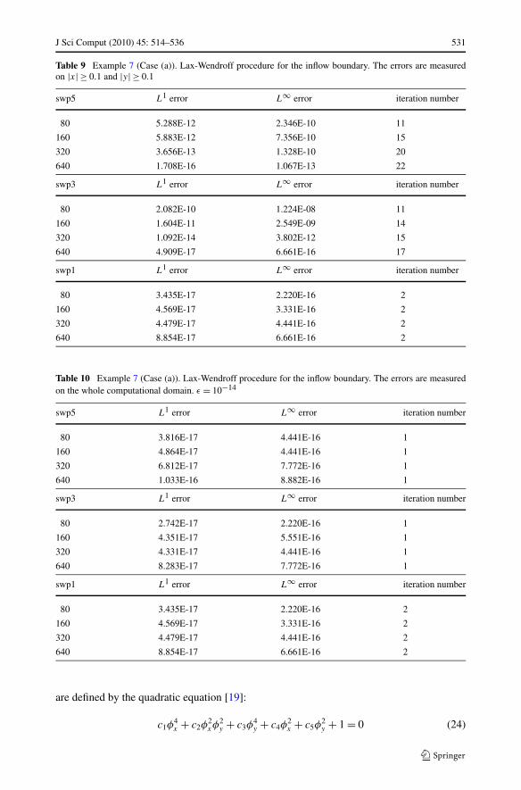
The results for Case (a) are listed in Table 9, where the errors are measured away fromthe two lines x = 0 and y = 0 along which the solution is not smooth. For this case, the

530 J Sci Comput (2010) 45: 514–536

Fig. 3 Example 6. The contours (top) and surfaces (bottom) of the numerical solution φ obtained with thefast sweeping fifth order WENO method. Case 1 (left) and Case 2 (right)

solution, away from the singularities along x = 0 and y = 0, is a bilinear polynomial, thusany scheme which is at least first order accurate with an exact boundary treatment shouldhave no truncation error and should produce only round-off level errors. If we use ε = 10−14

in the WENO nonlinear weights for “swp3” and “swp5”, which implies that we use the non-linear smoothness indicators down to the round off level in building the nonlinear weightsin the WENO schemes, allowing the WENO mechanism to completely avoid interpolatingacross the singularities along x = 0 and y = 0, we can actually obtain errors computed inthe whole computational domain down to the round-off level, as shown in Table 10.

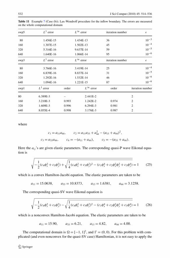
For Case (b), the solution is a polynomial with degree two, higher than first order butlower than third order, yielding first order error accuracy for “swp1” and round-off errorsfor “swp3” and “swp5”, when the same ε is chosen as in Example 6, as shown in Table 11.The numerical results obtained by the fast sweeping fifth order WENO method are displayedin Fig. 4.

Example 8 (Travel time problem in elastic wave propagation) This problem is from appli-cations such as the study of earthquakes. The quasi-P and the quasi-SV slowness surfaces

J Sci Comput (2010) 45: 514–536 531

Table 9 Example 7 (Case (a)). Lax-Wendroff procedure for the inflow boundary. The errors are measuredon |x| ≥ 0.1 and |y| ≥ 0.1

swp5 L1 error L∞ error iteration number

80 5.288E-12 2.346E-10 11

160 5.883E-12 7.356E-10 15

320 3.656E-13 1.328E-10 20

640 1.708E-16 1.067E-13 22


80 2.082E-10 1.224E-08 11

160 1.604E-11 2.549E-09 14

320 1.092E-14 3.802E-12 15

640 4.909E-17 6.661E-16 17


80 3.435E-17 2.220E-16 2

160 4.569E-17 3.331E-16 2

320 4.479E-17 4.441E-16 2

640 8.854E-17 6.661E-16 2

Table 10 Example 7 (Case (a)). Lax-Wendroff procedure for the inflow boundary. The errors are measuredon the whole computational domain. ε = 10−14


80 3.816E-17 4.441E-16 1

160 4.864E-17 4.441E-16 1

320 6.812E-17 7.772E-16 1

640 1.033E-16 8.882E-16 1


80 2.742E-17 2.220E-16 1

160 4.351E-17 5.551E-16 1

320 4.331E-17 4.441E-16 1

640 8.283E-17 7.772E-16 1


80 3.435E-17 2.220E-16 2

160 4.569E-17 3.331E-16 2

320 4.479E-17 4.441E-16 2

640 8.854E-17 6.661E-16 2

are defined by the quadratic equation [19]:

c1φ4x + c2φ

2xφ

2y + c3φ

4y + c4φ

2x + c5φ

2y + 1 = 0 (24)

532 J Sci Comput (2010) 45: 514–536

Table 11 Example 7 (Case (b)). Lax-Wendroff procedure for the inflow boundary. The errors are measuredon the whole computational domain

swp5 L1 error L∞ error iteration number ε

80 1.456E-15 1.434E-13 36 10−3

160 1.307E-15 1.502E-13 45 10−4

320 5.316E-16 9.637E-14 59 10−5

640 1.640E-16 1.066E-14 95 10−6

swp3 L1 error L∞ error iteration number ε

80 3.766E-16 3.419E-14 25 10−4

160 6.839E-16 8.837E-14 31 10−5

320 1.292E-16 1.532E-14 46 10−6

640 1.094E-16 1.221E-15 87 10−6

swp1 L1 error order L∞ error order iteration number

80 6.389E-3 – 2.441E-2 2

160 3.210E-3 0.993 1.242E-2 0.974 2

320 1.609E-3 0.996 6.294E-3 0.981 2

640 8.055E-4 0.998 3.176E-3 0.987 2

where

c1 = a11a44, c2 = a11a33 + a244 − (a13 + a44)

2,

c3 = a33a44, c4 = −(a11 + a44), c5 = −(a33 + a44).

Here the aij ’s are given elastic parameters. The corresponding quasi-P wave Eikonal equa-tion is √

−1

2(c4φ2

x + c5φ2y) +

√1

4(c4φ2

x + c5φ2y)

2 − (c1φ4x + c2φ2

xφ2y + c3φ4

y) = 1 (25)

which is a convex Hamilton-Jacobi equation. The elastic parameters are taken to be

a11 = 15.0638, a33 = 10.8373, a13 = 1.6381, a44 = 3.1258.

The corresponding quasi-SV wave Eikonal equation is

√−1

2(c4φ2

x + c5φ2y) −

√1

4(c4φ2

x + c5φ2y)

2 − (c1φ4x + c2φ2

xφ2y + c3φ4

y) = 1 (26)

which is a nonconvex Hamilton-Jacobi equation. The elastic parameters are taken to be

a11 = 15.90, a33 = 6.21, a13 = 4.82, a44 = 4.00.

The computational domain is � = [−1,1]2, and � = (0,0). For this problem with com-plicated (and even nonconvex for the quasi-SV case) Hamiltonian, it is not easy to apply the

J Sci Comput (2010) 45: 514–536 533

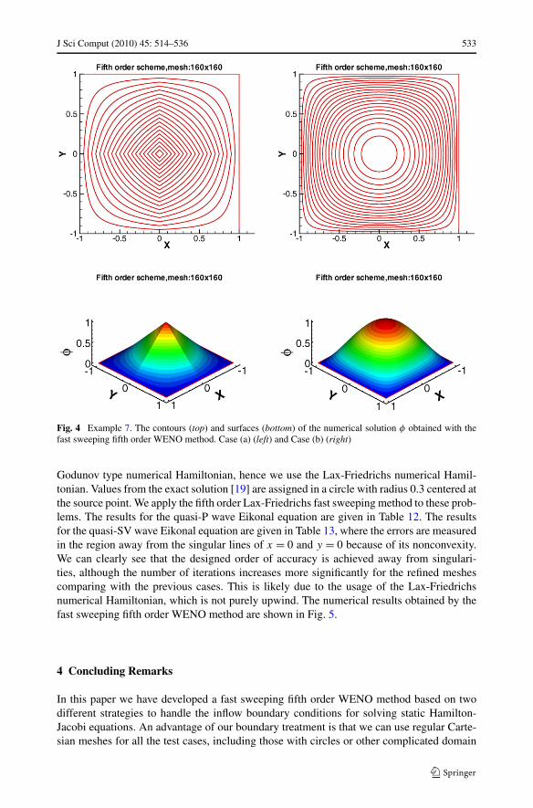
Fig. 4 Example 7. The contours (top) and surfaces (bottom) of the numerical solution φ obtained with thefast sweeping fifth order WENO method. Case (a) (left) and Case (b) (right)

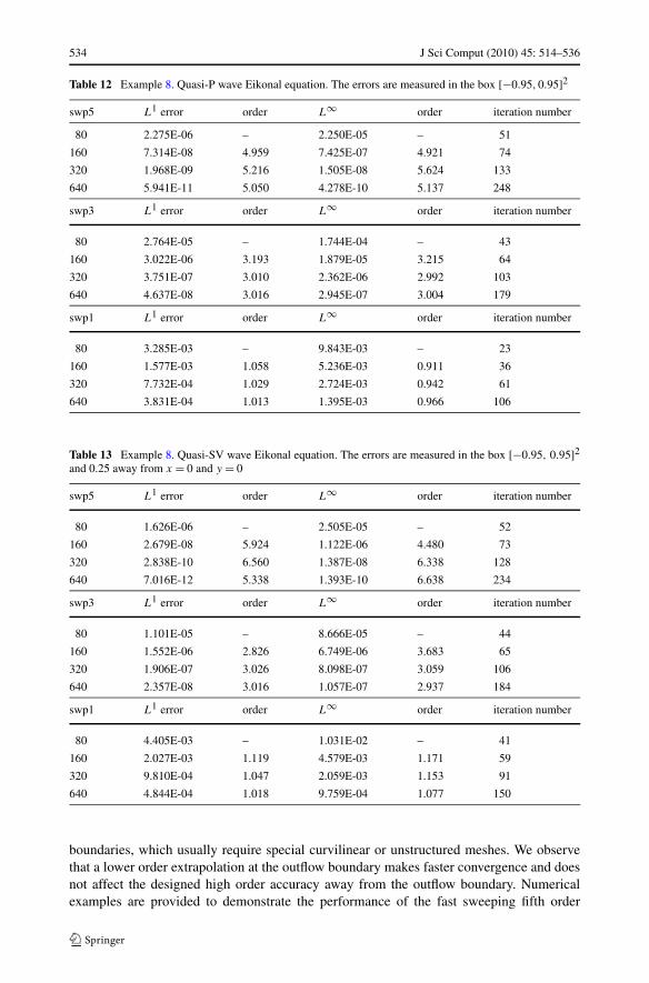
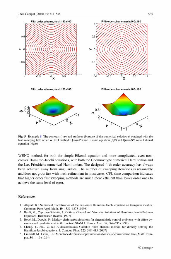
Godunov type numerical Hamiltonian, hence we use the Lax-Friedrichs numerical Hamil-tonian. Values from the exact solution [19] are assigned in a circle with radius 0.3 centered atthe source point. We apply the fifth order Lax-Friedrichs fast sweeping method to these prob-lems. The results for the quasi-P wave Eikonal equation are given in Table 12. The resultsfor the quasi-SV wave Eikonal equation are given in Table 13, where the errors are measuredin the region away from the singular lines of x = 0 and y = 0 because of its nonconvexity.We can clearly see that the designed order of accuracy is achieved away from singulari-ties, although the number of iterations increases more significantly for the refined meshescomparing with the previous cases. This is likely due to the usage of the Lax-Friedrichsnumerical Hamiltonian, which is not purely upwind. The numerical results obtained by thefast sweeping fifth order WENO method are shown in Fig. 5.

4 Concluding Remarks

In this paper we have developed a fast sweeping fifth order WENO method based on twodifferent strategies to handle the inflow boundary conditions for solving static Hamilton-Jacobi equations. An advantage of our boundary treatment is that we can use regular Carte-sian meshes for all the test cases, including those with circles or other complicated domain

534 J Sci Comput (2010) 45: 514–536

Table 12 Example 8. Quasi-P wave Eikonal equation. The errors are measured in the box [−0.95,0.95]2


80 2.275E-06 – 2.250E-05 – 51

160 7.314E-08 4.959 7.425E-07 4.921 74

320 1.968E-09 5.216 1.505E-08 5.624 133

640 5.941E-11 5.050 4.278E-10 5.137 248


80 2.764E-05 – 1.744E-04 – 43

160 3.022E-06 3.193 1.879E-05 3.215 64

320 3.751E-07 3.010 2.362E-06 2.992 103

640 4.637E-08 3.016 2.945E-07 3.004 179


80 3.285E-03 – 9.843E-03 – 23

160 1.577E-03 1.058 5.236E-03 0.911 36

320 7.732E-04 1.029 2.724E-03 0.942 61

640 3.831E-04 1.013 1.395E-03 0.966 106

Table 13 Example 8. Quasi-SV wave Eikonal equation. The errors are measured in the box [−0.95, 0.95]2and 0.25 away from x = 0 and y = 0


80 1.626E-06 – 2.505E-05 – 52

160 2.679E-08 5.924 1.122E-06 4.480 73

320 2.838E-10 6.560 1.387E-08 6.338 128

640 7.016E-12 5.338 1.393E-10 6.638 234


80 1.101E-05 – 8.666E-05 – 44

160 1.552E-06 2.826 6.749E-06 3.683 65

320 1.906E-07 3.026 8.098E-07 3.059 106

640 2.357E-08 3.016 1.057E-07 2.937 184


80 4.405E-03 – 1.031E-02 – 41

160 2.027E-03 1.119 4.579E-03 1.171 59

320 9.810E-04 1.047 2.059E-03 1.153 91

640 4.844E-04 1.018 9.759E-04 1.077 150

boundaries, which usually require special curvilinear or unstructured meshes. We observethat a lower order extrapolation at the outflow boundary makes faster convergence and doesnot affect the designed high order accuracy away from the outflow boundary. Numericalexamples are provided to demonstrate the performance of the fast sweeping fifth order

J Sci Comput (2010) 45: 514–536 535

Fig. 5 Example 8. The contours (top) and surfaces (bottom) of the numerical solution φ obtained with thefast sweeping fifth order WENO method. Quasi-P wave Eikonal equation (left) and Quasi-SV wave Eikonalequation (right)

WENO method, for both the simple Eikonal equation and more complicated, even non-convex Hamilton-Jacobi equations, with both the Godunov type numerical Hamiltonian andthe Lax-Friedrichs numerical Hamiltonian. The designed fifth order accuracy has alwaysbeen achieved away from singularities. The number of sweeping iterations is reasonableand does not grow fast with mesh refinement in most cases. CPU time comparison indicatesthat higher order fast sweeping methods are much more efficient than lower order ones toachieve the same level of error.

References

1. Abgrall, R.: Numerical discretization of the first-order Hamilton-Jacobi equation on triangular meshes.Commun. Pure Appl. Math. 49, 1339–1373 (1996)

2. Bardi, M., Capuzzo-Dolcetta, I.: Optimal Control and Viscosity Solutions of Hamilton-Jacobi-BellmanEquations. Birkhäuser, Boston (1997)

3. Boué, M., Dupuis, P.: Markov chain approximations for deterministic control problems with affine dy-namics and quadratic cost in the control. SIAM J. Numer. Anal. 36, 667–695 (1999)

4. Cheng, Y., Shu, C.-W.: A discontinuous Galerkin finite element method for directly solving theHamilton-Jacobi equations. J. Comput. Phys. 223, 398–415 (2007)

5. Crandall, M., Lions, P.L.: Monotone difference approximations for scalar conservation laws. Math. Com-put. 34, 1–19 (1984)

536 J Sci Comput (2010) 45: 514–536

6. Hu, C., Shu, C.-W.: A discontinuous Galerkin finite element method for Hamilton-Jacobi equations.SIAM J. Sci. Comput. 21, 666–690 (1999)

7. Huang, L., Shu, C.-W., Zhang, M.: Numerical boundary conditions for the fast sweeping high orderWENO methods for solving the Eikonal equation. J. Comput. Math. 26, 1–11 (2008)

8. Huang, L., Wong, S.C., Zhang, M., Shu, C.-W., Lam, W.H.K.: Revisiting Hughes’ dynamic continuummodel for pedestrian flow and the development of an efficient solution algorithm. Transp. Res. Part B,Methodol. 43, 127–141 (2009)

9. Jiang, G., Peng, D.P.: Weighted ENO schemes for Hamilton-Jacobi equations. SIAM J. Sci. Comput. 21,2126–2143 (2000)

10. Li, F., Shu, C.-W., Zhang, Y.-T., Zhao, H.: A second order discontinuous Galerkin fast sweeping methodfor Eikonal equations. J. Comput. Phys. 227, 8191–8208 (2008)

11. Osher, S., Sethian, J.: Fronts propagating with curvature dependent speed: algorithms based onHamilton-Jacobi formulations. J. Comput. Phys. 79, 12–49 (1988)

12. Osher, S., Shu, C.-W.: High-order essentially nonoscillatory schemes for Hamilton-Jacobi equations.SIAM J. Numer. Anal. 28, 907–922 (1991)

13. Rouy, E., Tourin, A.: A viscosity solutions approach to shape-from-shading. SIAM J. Numer. Anal. 29,867–884 (1992)

14. Serna, S., Qian, J.: A stopping criterion for higher-order sweeping schemes for static Hamilton-Jacobiequations. Preprint

15. Shu, C.-W.: High order numerical methods for time dependent Hamilton-Jacobi equations. In: Goh, S.S.,Ron, A., Shen, Z. (eds.) Mathematics and Computation in Imaging Science and Information Processing.Lecture Notes Series, Institute for Mathematical Sciences, National University of Singapore, vol. 11,pp. 47–91. World Scientific, Singapore (2007)

16. Shu, C.-W., Osher, S.: Efficient implementation of essentially non-oscillatory shock-capturing schemes.J. Comput. Phys. 77, 439–471 (1988)

17. Xia, Y., Wong, S.C., Zhang, M., Shu, C.-W., Lam, W.H.K.: An efficient discontinuous Galerkin methodon triangular meshes for a pedestrian flow model. Int. J. Numer. Methods Eng. 76, 337–350 (2008)

18. Zhang, Y.-T., Shu, C.-W.: High order WENO schemes for Hamilton-Jacobi equations on triangularmeshes. SIAM J. Sci. Comput. 24, 1005–1030 (2003)

19. Zhang, Y.-T., Zhao, H.-K., Qian, J.: High order fast sweeping methods for static Hamilton-Jacobi equa-tions. J. Sci. Comput. 29, 25–56 (2006)

20. Zhao, H.-K.: A fast sweeping method for Eikonal equations. Math. Comput. 74, 603–627 (2005)

Documents

Fast Sweeping Fifth Order WENO Scheme for Static …yzhang10/FS-WENO5.pdf · Fast Sweeping Fifth Order WENO Scheme for Static Hamilton-Jacobi Equations with Accurate Boundary