High order fast sweeping methods for static Hamilton ...zhao/publication/mypapers/pdf/FS_high... · High order fast sweeping methods for static Hamilton-Jacobi equations ... (WENO)

High order fast sweeping methods for static

Hamilton-Jacobi equations

Yong-Tao Zhang1, Hong-Kai Zhao2 and Jianliang Qian3

ABSTRACT

We construct high order fast sweeping numerical methods for computing viscosity solu-

tions of static Hamilton-Jacobi equations on rectangular grids. These methods combine high

order weighted essentially non-oscillatory (WENO) approximations to derivatives, monotone

numerical Hamiltonians and Gauss-Seidel iterations with alternating-direction sweepings.

Based on well-developed first order sweeping methods, we design a novel approach to in-

corporate high order approximations to derivatives into numerical Hamiltonians such that

the resulting numerical schemes are formally high order accurate and inherit the fast conver-

gence from the alternating sweeping strategy. Extensive numerical examples verify efficiency,

convergence and high order accuracy of the new methods.

Key Words: fast sweeping methods, WENO approximation, high order accuracy, static

Hamilton-Jacobi equations, Eikonal equations

1Department of Mathematics, University of California, Irvine, CA 92697-3875, USA. E-mail:

[email protected] of Mathematics, University of California, Irvine, CA 92697-3875, USA. E-mail:

[email protected]. The research is partially supported by ONR Grant #N00014-02-1-0090, DARPA Grant

#N00014-02-1-0603 and Sloan Fellowship Foundation.3Department of Mathematics, University of California, Los Angeles, CA 90095-1555, USA. E-mail:

[email protected]. Supported by ONR Grant #N00014-02-1-0720.

1

1 Introduction

We consider the static Hamilton-Jacobi equations

H(φx1, · · · , φxd

, x) = 0, x ∈ Ω \ Γ,

φ(x) = g(x), x ∈ Γ ⊂ Ω,(1.1)

where Ω is a computational domain in Rd and Γ is a subset of Ω. The Hamiltonian H is

a nonlinear Lipschitz continuous function. Such Hamilton-Jacobi (H-J) equations appear

in many applications, such as optimal control, differential games, image processing and

computer vision, and geometric optics.

A very important member of the family of the static Hamilton-Jacobi equations is the

Eikonal equation. The standard isotropic Eikonal equation is

|∇φ(x)| = f(x), x ∈ Ω \ Γ,

φ(x) = g(x), x ∈ Γ ⊂ Ω,(1.2)

where f(x) is a positive function.

Since the boundary value problems (1.1), (1.2) are nonlinear first order partial differential

equations, we may apply the classical method of characteristics to solve these equations in

phase space; namely, consider the gradient components as independent variables and solve

ODE systems to follow the propagation of characteristics. Although the characteristics may

never intersect in phase space, their projection into physical space may intersect so that the

solution in physical space is not uniquely defined at these intersections. By mimicking the

entropy condition for hyperbolic conservation laws to pick out a physically relevant solution,

Crandall and Lions [7] introduced the concept of viscosity solutions for Hamilton-Jacobi

equations so that a global, physically relevant solution can be defined for such first order

nonlinear equations. Moreover, monotone finite difference schemes are developed to compute

such viscosity solutions stably.

There are mainly two classes of numerical methods for solving static Hamilton-Jacobi

equations. The first class of numerical methods is based on reformulating the equations

into suitable time-dependent problems. Osher [22] provides a natural link between static

2

and time-dependent Hamilton-Jacobi equations by using the level-set idea and thus raising

the problem one-dimensional higher. The zero-level set of the viscosity solution ψ of the

time-dependent H-J equation

ψt +H(ψx1, · · · , ψxd

, x) = 0 (1.3)

at time t is the set of x such that φ(x) = t of (1.1), where the Hamiltonian H is homogeneous

of degree one. In the control framework, a semi-Lagrangian scheme is obtained for Hamilton-

Jacobi equations by discretizing in time the dynamic programming principle [9, 10]. Another

approach to obtaining a “time” dependent H-J equation from the static H-J equation is

using the so called paraxial formulation in which a preferred spatial direction is assumed

in the characteristic propagation [11, 8, 17, 27, 28]. High order numerical schemes are well

developed for the time dependent H-J equation (1.3) on structured and unstructured meshes

[24, 14, 39, 13, 23, 6, 16, 20, 25, 1, 2, 5, 4]; see a recent review on high order numerical methods

for time dependent H-J equations by Shu [35]. Due to the finite speed of propagation and

the CFL condition for the discrete time step size, the number of time steps has to be of the

same order as that for one of the spatial dimensions so that the solution converges in the

entire domain.

The other class of numerical methods for static H-J equations is to treat the problem

as a stationary boundary value problem: discretize the problem into a system of nonlinear

equations and design an efficient numerical algorithm to solve the system. Among such

methods are the fast marching method and the fast sweeping method. In the fast marching

method [38, 32, 12, 33, 34], the solution is updated by following the causality in a sequential

way; i.e., the solution is updated pointwise in the order that the solution is strictly increas-

ing (decreasing); hence two essential ingredients are needed in the algorithm: an upwind

difference scheme and a heap-sort algorithm. The resulting complexity of the fast marching

method is of order O(N logN) for N grid points, where the logN factor comes from the

heap-sort algorithm. In the fast sweeping method [3, 41, 37, 40, 18, 19], Gauss-Seidel itera-

tions with alternating direction sweepings are incorporated into upwind finite differences. In

3

contrast to the fast marching method, the fast sweeping method follows the causality along

characteristics in a parallel way; i.e., all characteristics are divided into a finite number of

groups according to their directions and each Gauss-Seidel iteration with a specific sweeping

ordering covers a group of characteristics simultaneously; no heap-sort is needed. The fast

sweeping method is optimal in the sense that a finite number of iterations is needed [40], so

that the complexity of the algorithm is O(N) for a total of N grid points; i.e., the number of

iterations is independent of the grid size. The algorithm is extremely simple to implement.

Both the fast marching method and the fast sweeping method are extremely efficient

algorithms for solving static Hamilton-Jacobi equations. In fact both of them solve the

same system of discretized equations and try to order the nonlinear system of equations

following the causality along characteristics. Here we point out a few interesting differences

between these two methods. For the complexity, the fast marching method is O(N logN)

and the fast sweeping method is O(N). However the constant in the complexity for the fast

marching method does not depend on the equation while the constant in the complexity for

the fast sweeping method depends on the equation (but not on the grid size) [40]. On a

given discretization which method is faster depends on the equation. In practice they are

more or less comparable. As to the ordering philosophy these two methods are different.

The fast marching method sorts out the ordering on the fly using the heap-sort algorithm;

a strict causality principle has to exist and to be enforced to order the equations; i.e.,

equations solved later has no influence on the previous equations. On the other hand, the

fast sweeping method is in the general framework of iterative methods. If a strict causality

exists (such as in Eikonal equations), it can be enforced in the iterative procedure, which

guarantees convergence in a finite number of alternating sweepings. Therefore, the iterative

framework is more robust and flexible for general equations and high order methods. With

alternating ordering, the iterations can follow causality along characteristics, and handle

global relaxation and smoothing effects as well. For examples, even if there is no strict

causality, such as when the Hamiltonian is not convex, or there are viscosity terms (e.g. the

4

solutions are coupled globally), or the numerical method (e.g., high order method) is not

monotone, it is still possible that the iteration will converge. Another interesting remark is

on the convergence mechanism for iterative methods. In general the convergence of iterative

methods is due to a certain contraction property as in the fixed point iteration. Infinite

number of iterations are needed for full convergence. When a strict causality exists and is

enforced in the fast sweeping method as in Eikonal equations, the convergence is achieved

in a finite number of iterations due to the alternating sweeping order. In general different

sweeping orders will not change the contraction property of an iterative method. So both

mechanisms can be in effect in more general situations.

In many applications, the numerical solutions from H-J equations are used to compute

other quantities and thus their numerical derivatives are needed as well; for example, in

geometrical optics the derivatives of travel-times are used to compute amplitudes [29]. In

this paper we develop a quite general framework for constructing high order fast sweeping

methods. We adapt high order schemes for time dependent Hamilton-Jacobi equations in

[24, 14, 39] to the static H-J equations in a novel way. First-order sweeping schemes are

used as building blocks in our high order methods. The high order accuracy in our schemes

results from the high order approximations for the partial derivatives because the monotone

numerical Hamiltonians are Lipschitz continuous and consistent with the Hamiltonian H in

the PDEs. In particular, we use the WENO approximations [14, 15], since the weighted

essentially non-oscillatory (WENO) approximations have uniform high order accuracy, and

are more robust and efficient than other schemes such as ENO schemes.

The algorithm is developed in Section 2. First we describe the algorithm for the Eikonal

equation, then we extend it to the general static Hamilton-Jacobi equations. In Section 3,

extensive numerical experiments are performed to demonstrate accuracy and fast convergence

of the algorithms. High order accuracy in smooth regions and good resolution of derivative

singularities are observed. Concluding remarks are given in Section 4.

5

2 High order sweeping methods

We consider the two dimensional problems for simplicity. The extension to higher dimensions

is straightforward.

2.1 Principles for constructing sweeping methods

To compute the viscosity solution for equation (1.1), we first discretize the domain Ω. Sup-

pose that a rectangular mesh Ωh covers the computational domain Ω. Let (i, j) denote a

grid point in Ωh, i.e., Ωh = (i, j), 1 ≤ i ≤ I, 1 ≤ j ≤ J, and φi,j denote the numerical

solution at the grid point (i, j). hx and hy denote uniform grid sizes in the x-direction and

the y-direction respectively; to simplify the notation, we take hx = hy = h.

Next we discretize the Hamiltonian H by a monotone numerical Hamiltonian H [24]:

H(φ−

x , φ+x ;φ−

y , φ+y )ij = 0, (i, j) ∈ Ωh \ Γh,

φij = gij, (i, j) ∈ Γh ⊂ Ωh.(2.1)

Since the H-J equation is in general nonlinear, we end up with a coupled nonlinear system

for unknown solutions at those mesh points. Because the boundary values are usually given

on irregular geometries, it is very involved to solve the nonlinear system globally. Therefore,

we appeal to construct an iterative method based to local solvers. An essential ingredient

for constructing a sweeping method is an efficient local solver which expresses the value at

the standing mesh point in terms of its neighboring values. If the Godunov’s Hamiltonian

is the numerical Hamiltonian in equation (2.1), then it is straightforward to carry out the

local solution procedure for the eikonal equation (1.2); in fact, the popularity of the Fast

Marching method [38, 32] and Fast Sweeping method [40] is more or less due to such efficient

local solvers. Furthermore, if the Godunov’s Hamiltonian is the numerical Hamiltonian in

equation (2.1), then it is also possible to carry out the local solution procedure for H-J

equations (1.2) with convexity in the gradient component of Hamiltonians; see [37]. But if

the Hamiltonian is non-convex in the gradient component, then it is extremely involved to

carry out the minmax optimization resulting from the Godunov monotone Hamiltonian. On

6

the other hand, if the Lax-Friedrichs Hamiltonian is utilized, then it is extremely simple to

carry out the local solution process, no matter whether the Hamiltonian is convex or not,

no matter how complicated the Hamiltonian could be; see [18]. In passing, we note that

it is also possible to use the Roe-entropy fix type numerical Hamiltonian to discretize the

H-J equation, and it is expected that the resulting scheme will interpolate the behavior of

Godunov and Lax-Friedrichs schemes.

Once a local solver is in place, symmetrical Gauss-Seidel nonlinear iterative methods can

be applied immediately to obtain efficient fast sweeping methods.

2.2 Eikonal equations

We take d = 2 in (1.2):

√

φ2x + φ2

y = f(x, y), (x, y) ∈ Ω ⊂ R2,

φ(x, y) = g(x, y), (x, y) ∈ Γ ⊂ Ω.(2.2)

A first-order Godunov upwind difference scheme is used to discretize the PDE (2.2) as

in [40]:

[(φi,j − φ

(xmin)i,j

h)+]2 + [(

φi,j − φ(ymin)i,j

h)+]2 = f 2

i,j, (2.3)

where φ(xmin)i,j = min(φi−1,j, φi+1,j), φ

(ymin)i,j = min(φi,j−1, φi,j+1) and

(x)+ =

x, x > 0,

0, x ≤ 0.(2.4)

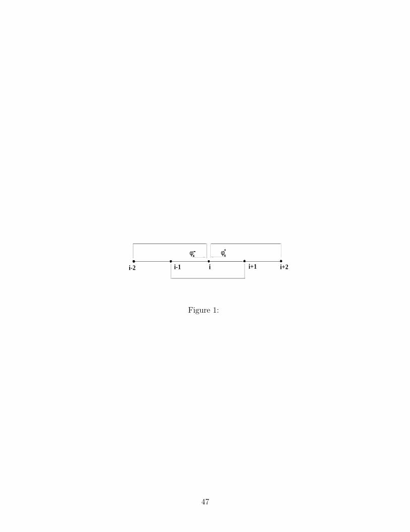
In order to construct a higher order scheme, we need to approximate the derivatives φx

and φy with high order accuracy. We choose to use the popular WENO approximations

developed in [14, 15]. To illustrate the feasibility of the approach, we take the third order

rather than the fifth order WENO approximations; one certainly can replace the third order

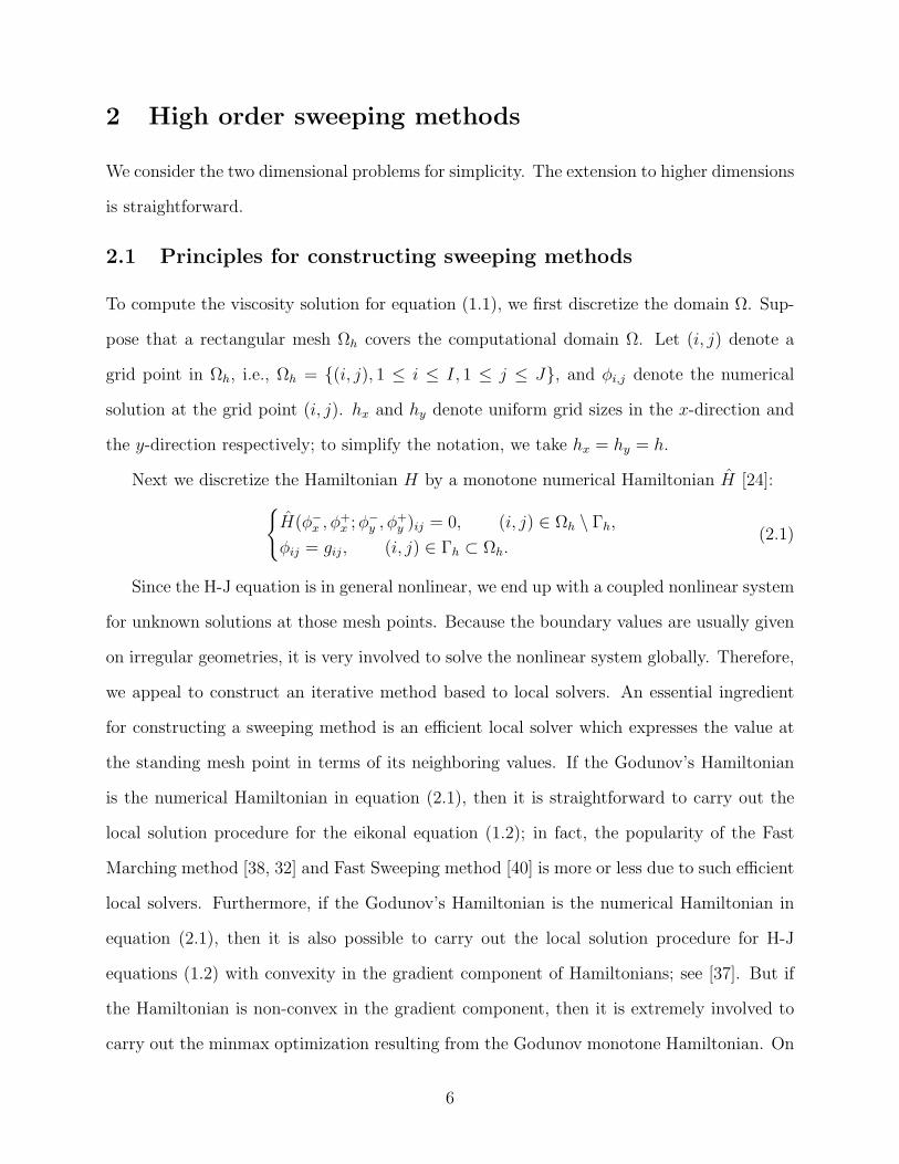
WENO with the fifth order or even higher order WENO approximations. The interpolation

stencil for the third order WENO scheme is shown in Figure 1. (φx)i,j and (φy)i,j denote

approximations for φx and φy at the grid point (i, j), respectively. The approximation for

φx at the grid point (i, j) when the wind “blows” from the left to the right is

(φx)−

i,j = (1 − w−)(φi+1,j − φi−1,j

2h) + w−(

3φi,j − 4φi−1,j + φi−2,j

2h), (2.5)

7

where

w− =1

1 + 2r2−

, r− =ǫ+ (φi,j − 2φi−1,j + φi−2,j)

2

ǫ+ (φi+1,j − 2φi,j + φi−1,j)2; (2.6)

on the other hand, the approximation for φx at the grid point (i, j) when the wind “blows”

from the right to the left is

(φx)+i,j = (1 − w+)(

φi+1,j − φi−1,j

2h) + w+(

−φi+2,j + 4φi+1,j − 3φi,j

2h), (2.7)

where

w+ =1

1 + 2r2+

, r+ =ǫ+ (φi+2,j − 2φi+1,j + φi,j)

2

ǫ+ (φi+1,j − 2φi,j + φi−1,j)2. (2.8)

Similarly we define (φy)−

i,j and (φy)+i,j.

Next we have to incorporate these high order approximations (2.5)-(2.8) for derivatives

into monotone numerical Hamiltonians. In the case of eikonal equations, the numerical

Hamiltonian under consideration is (2.3). In order to achieve this, we notice that the follow-

ing identities hold:

(φx)−

i,j =φi,j − [φi,j − h · (φx)

−

i,j]

h, (φx)

+i,j =

[φi,j + h · (φx)+i,j] − φi,j

h, (2.9)

(φy)−

i,j =φi,j − [φi,j − h · (φy)

−

i,j]

h, (φy)

+i,j =

[φi,j + h · (φy)+i,j] − φi,j

h. (2.10)

According to the definitions of (φx)−

i,j and (φx)+i,j, φi,j − h · (φx)

−

i,j can be considered as an

approximation to φi−1,j while φi,j +h ·(φx)+i,j can be considered as an approximation to φi+1,j.

Similarly in (2.10), φi,j −h ·(φy)−

i,j and φi,j +h ·(φy)+i,j can be considered as approximations to

φi,j−1 and φi,j+1, respectively. Replacing φi−1,j, φi+1,j, φi,j−1, φi,j+1 with these approximations

in equation (2.3), we have the following higher order schemes,

[(φnew

i,j − φ(xmin)i,j

h)+]2 + [(

φnewi,j − φ

(ymin)i,j

h)+]2 = f 2

i,j (2.11)

where

φ(xmin)i,j = min(φold

i,j − h · (φx)−

i,j, φoldi,j + h · (φx)

+i,j),

φ(ymin)i,j = min(φold

i,j − h · (φy)−

i,j, φoldi,j + h · (φy)

+i,j).

(2.12)

Here φnewi,j denotes the to-be-updated numerical solution for φ at the grid point (i, j), and φold

i,j

denotes the current old value for φ at the same grid point. When WENO approximations for

8

derivatives (φx)−

i,j, (φx)+i,j, (φy)

−

i,j, (φy)+i,j in (2.12) are computed according to formulae (2.5)-

(2.8), we always use the newest available values for φ in the interpolation stencils according

to the philosophy of Gauss-Seidel type iterations. Of course, since we have not updated φi,j

yet, φoldi,j is used in (2.5)-(2.8). The solution for equation (2.11) is:

φnewi,j =

min(φ(xmin)i,j , φ

(ymin)i,j ) + fi,jh, |φ(xmin)

i,j − φ(ymin)i,j | ≥ fi,jh,

φ(xmin)i,j + φ

(ymin)i,j +

√

2f 2i,jh

2 − (φ(xmin)i,j − φ

(ymin)i,j )2

2, otherwise.

(2.13)

Remark 1. We introduce the high order accuracy by replacing φi−1,j, φi+1,j, φi,j−1, φi,j+1

with φi,j − h · (φx)−

i,j, φi,j + h · (φx)+i,j, φi,j − h · (φy)

−

i,j, φi,j + h · (φy)+i,j, respectively, where

(φx)−


−

i,j, (φy)+i,j are higher order WENO approximations for partial derivatives.

When the iterations converge, we have solved the system

√

max[(φx)−

i,j]+, [−(φx)

+i,j]

+2 + max[(φy)−

i,j]+, [−(φy)

+i,j]

+2 = fi,j, 1 ≤ i ≤ I, 1 ≤ j ≤ J.

(2.14)

Since the Godunov numerical Hamiltonian is Lipschitz continuous with respect to all of its

arguments, i.e., all of these high order approximations for partial derivatives, our schemes

achieve the same formal higher order accuracy as the approximations for partial derivatives

do.

Remark 2. The first order Godunov fast sweeping scheme (2.3) is purely upwind and mono-

tone, hence the fast convergence is guaranteed (see [40]). There is no such monotonicity for

the higher order scheme (2.11)-(2.12). A reliable initial guess is needed for the fast conver-

gence of the Gauss-Seidel iterations. In other words, to achieve fast convergence we wish to

have φi,j − h · (φx)−

i,j, φi,j + h · (φx)+i,j, φi,j − h · (φy)

−

i,j, φi,j + h · (φy)+i,j as good approximations

to φi−1,j, φi+1,j, φi,j−1, φi,j+1, respectively, so that the causality of the true solution is approx-

imately right. In the implementations of Godunov based high order fast sweeping schemes,

we use the first order Godunov fast sweeping scheme, which is robust and efficient, to provide

a good initial guess. Since the first order Godunov fast sweeping scheme converges in just a

few iterations, it is efficient to initialize the solution by such a scheme.

9

We summarize the higher order Godunov fast sweeping method for the eikonal equation

(2.2) as follows:

1. Initialization: according to the boundary condition φ(x, y) = g(x, y), (x, y) ∈ Γ,

assign exact values or interpolated values at grid points whose distances to Γ are

less than or equal to (n − 1)h, where n is the number of grid points in the small

stencil in WENO approximations. For example, n = 3 for the third order WENO

approximations. These values are fixed during iterations. The solution from the first-

order Godunov fast sweeping method is used as the initial guess at all other grid

points.

2. Iterations: solve the discretized nonlinear system (2.11) by Gauss-Seidel iterations with

four alternating direction sweepings:

(1) i = 1 : I, j = 1 : J ;

(2) i = I : 1, j = 1 : J ;

(3) i = I : 1, j = J : 1;

(4) i = 1 : I, j = J : 1.

Equations (2.5)-(2.8) and equations (2.12), (2.13) are used to solve (2.11). High order

extrapolations are used for the ghost points when calculating the high order WENO

approximations of derivatives (2.5)-(2.8) for grid points on the boundary of the com-

putational domain.

3. Convergence: if

||φnew − φold||L1 ≤ δ,

where δ is a given convergence threshold value and || · || denotes the L1 norm, the

algorithm converges and stops.

10

Remark 3. In the first order fast sweeping method [40], at each grid point (i, j), when the

solution, denoted by φ, of (2.3) is calculated from the current values of its neighboring grid

points, φnewi,j = min(φold

i,j , φ) is enforced so that the solution at each grid point is monotonically

decreasing from an initially assigned large value. The reason for imposing this condition is

that the first order scheme is monotone, thus the numerical solution at any iteration can not

get smaller than the numerical steady state solution for the discretized nonlinear system.

However, for higher order schemes there is no such monotonicity any more. The solution

may oscillate around the steady state solution. The oscillations are small. However, we can

NOT force φnewi,j = min(φold

i,j , φ) as in the first order scheme. Otherwise, the order of accuracy

of the schemes will deteriorate. Our numerical experiments have verified this.

Remark 4. In general the solution of this nonlinear PDE is not smooth. So the high order

accuracy of our numerical schemes may not be achieved at singularities. However, the main

issue is whether the breakdown at singularities will pollute the whole solution since errors

can propagate along characteristics. There are two different scenarios for this issue. If

the singularities are caused by the collision of characteristics analogous to the formation of

shocks in hyperbolic conservation laws, the errors incurred at these singularities will not

pollute solutions in other regions since no characteristics flow out of such singularities. If

there are characteristics flowing out of the the singularities analogous to rarefaction waves in

hyperbolic conservation laws, there will be pollution effects in the rarefaction wave region and

more refined meshes are needed near these singularities to achieve uniform error bounds; see

[29]. For the boundary value problem (2.2) all characteristics emanate from the boundary

Γ. If there are singularities, such as corners or point sources, from which characteristics

emanate, we assign exact solutions to a fixed local domain around those singularities when

we refine the mesh, so that the high order convergence of the scheme can be observed. The

above observation will be verified and discussed in more detail in the section for numerical

examples.

Remark 5. Another important issue is to compare the computational cost of our higher

11

order methods with that of the first order method. Suppose that the number of grids in

each direction is N and the space dimension is d for the pth order method. To achieve the

same accuracy for a first order method, we need Np grid points in each direction. Since the

first order method converges in a finite number of iterations independent of grid size, the

computation cost is O(Npd). So as long as the number of iterations for the pth order method

does not grow faster than N (p−1)d, we reduce the computational cost by using the high order

method. For example, if we take the third order method in two dimensions, we can see from

our numerical examples in section 3 that the number of iterations is far fewer than N4.

2.3 General static Hamilton-Jacobi equations

The idea of constructing high order sweeping methods for Eikonal equations can be straight-

forwardly extended to general static Hamilton-Jacobi equations

H(φx, φy) = f(x, y), x ∈ Ω \ Γ,

φ(x, y) = g(x, y), x ∈ Γ ⊂ Ω.(2.15)

To discretize a general Hamiltonian H(φx, φy), we may use the Lax-Friedrichs numerical

Hamiltonian [24] which is the simplest among all monotone numerical Hamiltonians:

HLF (u−, u+; v−, v+) = H(u− + u+

2,v− + v+

2) − 1

2αx(u+ − u−) − 1

2αy(v+ − v−) (2.16)

where

αx = maxA≤u≤BC≤v≤D

|H1(u, v)|, αy = maxA≤u≤BC≤v≤D

|H2(u, v)|. (2.17)

Here Hi(u, v) is the partial derivative of H with respect to the i-th argument, or the Lipschitz

constant of H with respect to the i-th argument. [A,B] is the value range for u±, and [C,D]

is the value range for v±.

Kao, Osher and Qian constructed the first order Lax-Friedrichs sweeping schemes for

general static Hamilton-Jacobi equations in [18]

φnewi,j =

(

1αx

hx+ αy

hy

)

[

f −H

(

φi+1,j − φi−1,j

2hx

,φi,j+1 − φi,j−1

2hy

)

+αx

φi+1,j + φi−1,j

2hx

+ αy

φi,j+1 + φi,j−1

2hy

]

. (2.18)

12

Following the idea in Section (2.2), we replace φi−1,j, φi+1,j, φi,j−1 and φi,j+1 with φi,j − hx ·

(φx)−

i,j, φi,j + hx · (φx)+i,j, φi,j − hy · (φy)

−

i,j and φi,j + hy · (φy)+i,j, respectively, in (2.18), where

(φx)−


−

i,j, and (φy)+i,j are higher order WENO approximations for partial deriva-

tives of φ. Then the high order Lax-Friedrichs sweeping schemes for static H-J equations

can be written as

φnewi,j =

(

1αx

hx+ αy

hy

)[

f −H

(

(φx)−

i,j + (φx)+i,j

2,(φy)

−

i,j + (φy)+i,j

2

)

+αx

2φoldi,j + hx((φx)

+i,j − (φx)

−

i,j)

2hx

+ αy

2φoldi,j + hy((φy)

+i,j − (φy)

−

i,j)

2hy

]

, (2.19)

or, written more compactly,

φnewi,j =

(

1αx

hx+ αy

hy

)[

f −H

(

(φx)−

i,j + (φx)+i,j

2,(φy)

−

i,j + (φy)+i,j

2

)

+αx

(φx)+i,j − (φx)

−

i,j

2+ αy

(φy)+i,j − (φy)

−

i,j

2

]

+ φoldi,j , (2.20)

where φnewi,j denotes the to-be-updated numerical solution for φ at the grid point (i, j), and

φoldi,j denotes the current old value for φ at the same grid point. When WENO approximations

for derivatives (φx)−


−

i,j, (φy)+i,j in (2.20) are calculated using formulae (2.5)-(2.8),

we always use the newest value that we currently have for φ in the interpolation stencils

according to the Gauss-Seidel type iteration. Of course, since we have not updated φi,j yet,

φoldi,j is used in (2.5)-(2.8).

Since the Lax-Friedrichs numerical Hamiltonian is not a purely upwind flux, the causality

along the characteristics is not strictly enforced. Thus the Lax-Friedrichs sweeping may take

more iterations than the Godunov sweeping in general. However, it is easy to implement the

Lax-Friedrichs Hamiltonians for more general equations. From our numerical experiments,

the Lax-Friedrichs high order sweeping is more robust with respect to the initial guess than

the Godunov high order sweeping. In our implementations we use big values, rather than

the results from the first order Lax-Friedrichs fast sweeping method, as the initial guess in

the high-order Lax-Friedrichs fast sweeping methods. The number of iterations is almost the

same as the first order version in [18].

13

The high order Lax-Friedrichs fast sweeping methods for general static Hamilton-Jacobi

equations are summarized as follows:

1. Initialization: according to the boundary condition φ(x, y) = g(x, y), (x, y) ∈ Γ,

assign exact values or interpolated values at grid points whose distances to Γ are

less than or equal to (n − 1)h, where n is the number of grid points in the small

stencil in WENO approximations. For example, n = 3 for the third order WENO

approximations. These values are fixed during iterations. Big values are used as the

initial guess at all other grid points.

2. Iterations: update φnewi,j in (2.20) by Gauss-Seidel iterations with four alternating di-

rection sweepings:

(1) i = 1 : I, j = 1 : J ;

(2) i = I : 1, j = 1 : J ;

(3) i = I : 1, j = J : 1;

(4) i = 1 : I, j = J : 1.

WENO approximations (2.5)-(2.8) are used in (2.20). Linear Extrapolations are used

for the ghost points when calculating the high order WENO approximations of deriva-

tives (2.5)-(2.8) for grid points on the boundary of the computational domain.

3. Convergence: if

||φnew − φold||L1 ≤ δ,

where δ is a given convergence threshold value, the algorithm converges and stops.

Remark 6. High order approximations for derivatives can also be incorporated into other

monotone numerical Hamiltonians in the same way as done here for Godunov and Lax-

Friedrichs numerical Hamiltonians.

Remark 7. From our numerical experiments, the iterations needed for the Godunov based

high order scheme to converge are fewer than those for the Lax-Friedrichs based high order

14

scheme; however, which one to choose really depends on how easy to carry out the local

solution procedure.

Remark 8. In our implementation for the third order Lax-Friedrichs sweeping scheme, we

use linear extrapolation at the boundary points if there is no prescribed influx or other

boundary conditions. It seems that high order extrapolations with bad initial guesses may

cause instability because the causality along characteristics may not be followed correctly

and no monotonicity exists for high order extrapolations. If the information is flowing out

of the boundary, the low order accuracy at the boundary will not affect the accuracy in the

interior, and the boundary points are excluded when we measure the error of our numerical

solutions. But for the high order Godunov sweeping scheme, the initial guesses are the

solutions from the first order scheme, so high order extrapolation boundary conditions are

very robust. A fourth order extrapolation boundary condition is used in our implementation

for the third order Godunov sweeping scheme.

3 Numerical Examples

We apply the high order fast sweeping methods to some typical two dimensional and three

dimensional problems. Third order WENO approximations are used. In all the examples,

the threshold value at which the iteration stops is taken to be δ = 10−11. One iteration

count includes four alternating sweepings for two dimensional problems and eight alternating

sweepings for three dimensional problems.

Example 1. Eikonal equation (2.2) with

f(x, y) =π

2

√

sin2(π +π

2x) + sin2(π +

π

2y), (3.1)

and Γ is the point (0, 0). The computational domain is [−1, 1]× [−1, 1]. The exact solution

for this problem is

φ(x, y) = cos(π +π

2x) + cos(π +

π

2y). (3.2)

15

The Godunov Hamiltonian is used. Since the solution is smooth, errors and convergence

rates in Table 1 indicate that the third order accuracy is obtained in the whole domain.

Example 2. Eikonal equation (2.2) with f(x, y) = 1. The computational domain is

Ω = [−1, 1] × [−1, 1], and Γ is a circle of center (0, 0) and radius 0.5. The exact solution

is the distance function to the circle Γ; thus the solution has a singularity at the center of

the circle to which the characteristics converge. The Godunov Hamiltonian is used. Table 2

shows the errors and the third order accuracy in the smooth region (0.15 distance away from

the center) of the solution. Table 3 shows the accuracy for the whole domain. Because of

the singularity in the solution, the scheme achieves only the first order accuracy in the L∞

norm; however, the L1 accuracy for the whole domain still indicates the third order accuracy

because the first order error is only made at the center (which is of measure O(h2)) and

there is no pollution effect. This indicates that the L1 norm might be a more appropriate

measure for the convergence rate of approximate solutions than the L∞ norm. Theoretically,

this was concluded by Lin-Tadmor [21].

Example 3. Case 1. 2-D Eikonal equation (2.2) with f(x, y) = 1.

The computational domain is Ω = [−3, 3] × [−3, 3]; Γ consists of two circles of equal

radius 0.5 with centers located at (−1, 0) and (√

1.5, 0), respectively. The exact solution is

the distance function to Γ. The singular set for the solution is composed of the center of

each circle and the line that is equally distant to the two circles. All of these singularities

correspond to the intersection of characteristics. The Godunov Hamiltonian is used. Table

4 shows that the third order accuracy is obtained in the smooth region, where the errors are

measured 0.15 distance away from the singular set. Table 5 shows that the scheme achieves

only the first order accuracy in the L∞ norm due to the singularity in the solution; moreover,

the L1 error in the whole domain indicates the second order accuracy since the singular set

has a measure of O(h).

Case 2. The 3-D eikonal equation.

Following the idea of high order fast sweeping algorithms for two dimensional problems in

16

Section 2, we can construct the algorithms for three dimensional problems straightforwardly.

For example, consider the 3-D eikonal equation

√

φ2x + φ2

y + φ2z = f(x, y, z), (x, y, z) ∈ Ω ⊂ R3,

φ(x, y, z) = g(x, y, z), (x, y, z) ∈ Γ ⊂ Ω.(3.3)

The local solver by the Godunov numerical Hamiltonian is

[(φnew

i,j − φ(xmin)i,j

h)+]2 + [(

φnewi,j − φ

(ymin)i,j

h)+]2 + [(

φnewi,j − φ

(zmin)i,j

h)+]2 = f 2

i,j (3.4)

where

φ(xmin)i,j = min(φold

i,j − h · (φx)−

i,j, φoldi,j + h · (φx)

+i,j),

φ(ymin)i,j = min(φold

i,j − h · (φy)−

i,j, φoldi,j + h · (φy)

+i,j),

φ(zmin)i,j = min(φold

i,j − h · (φz)−

i,j, φoldi,j + h · (φz)

+i,j).

(3.5)

(φx)−


−

i,j, (φy)+i,j, (φz)

−

i,j, (φz)+i,j are the WENO approximations for left and right

derivatives in x, y, z directions. The discretized nonlinear system (3.4) is solved by the sys-

tematic method in [40] and Gauss-Seidel iterations with eight alternating direction sweepings.

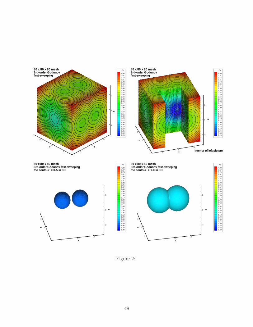
We use the two-sphere problem to test the third order algorithm for three dimensional prob-

lems. The computational domain is Ω = [−3, 3]× [−3, 3]× [−3, 3]; Γ consists of two spheres

of equal radius 0.5 with centers located at (−1, 0, 0) and (√

1.5, 0, 0), respectively. The ac-

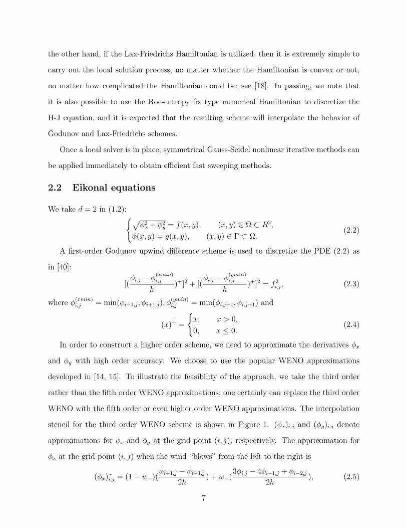
curacy for the whole domain and iteration numbers are listed in Table 6, and the contour

plots of the solution by a 80× 80 × 80 mesh are presented in Figure 2 for the surface of the

domain, a part of the interior of the domain and in the cases of two contour values 0.5 and

1.0 in the 3-D case, respectively. Similar conclusions as in the 2-D example can be drawn

here.

Example 4. Eikonal equation (2.2) with f(x, y) = 1. The Godunov Hamiltonian is

used. The computational domain is Ω = [−1, 1] × [−1, 1], and Γ is a source point with

coordinates (0, 0). So the exact solution is the distance function to the source point Γ. The

solution is singular at the source point. Since all characteristics emanate from this source

point analogous to rarefaction waves in hyperbolic conservation laws, errors incurred at the

source point will propagate out and pollute the solution in the whole computational domain.

17

We illustrate this subtlety with different initializations near the source point. This was also

treated in the geometrical optics setting in [29].

First we assign the exact values to a small region which encloses the source point, say, a

small box with length 0.3. This box size is fixed during the mesh refinement study. Accuracy

and errors are reported in Table 7, and the third order accuracy is obtained.

Next we initialize the solution near the source point by fixing the number of grid points

during the mesh refinement study. Thus the box which encloses the source point is taken

to have length 2h, where h is the mesh size. Accuracy and errors are reported in Table 8,

and the third order accuracy is polluted to some extent. We remark that in Example 2 and

Example 3 where singularities are of shock type, both of the two initializations led to neat

third order accuracy. The reason is that the rarefaction wave is different from the shock wave.

Characteristics intersect to form shocks. Errors incurred at the shocks will not propagate

from shocks to other locations to degrade the high order accuracy of the solution in smooth

regions. But if Γ has source points or corners from which the characteristics emanate so

that the rarefaction wave forms, the errors incurred at the singular point will propagate to

pollute the solution in the smooth region, hence leading to the loss of accuracy. Of course,

if a small fixed domain is used to wrap up the singular corner point, i.e., accurate values are

assigned to the small region, the high order accuracy can be achieved. The most efficient way

to recover such a loss of accuracy is to use adaptive meshes with good a posteriori estimates

near singularities; see [29] for such an adaptive method in the paraxial formulation.

In Table 9, we also list the errors and convergence rates for the first order fast sweeping

method (2.3). In comparison with the results in Table 7 and 8, the high order schemes do

achieve much smaller errors than a low order method does on the same grids.

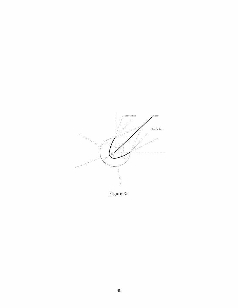
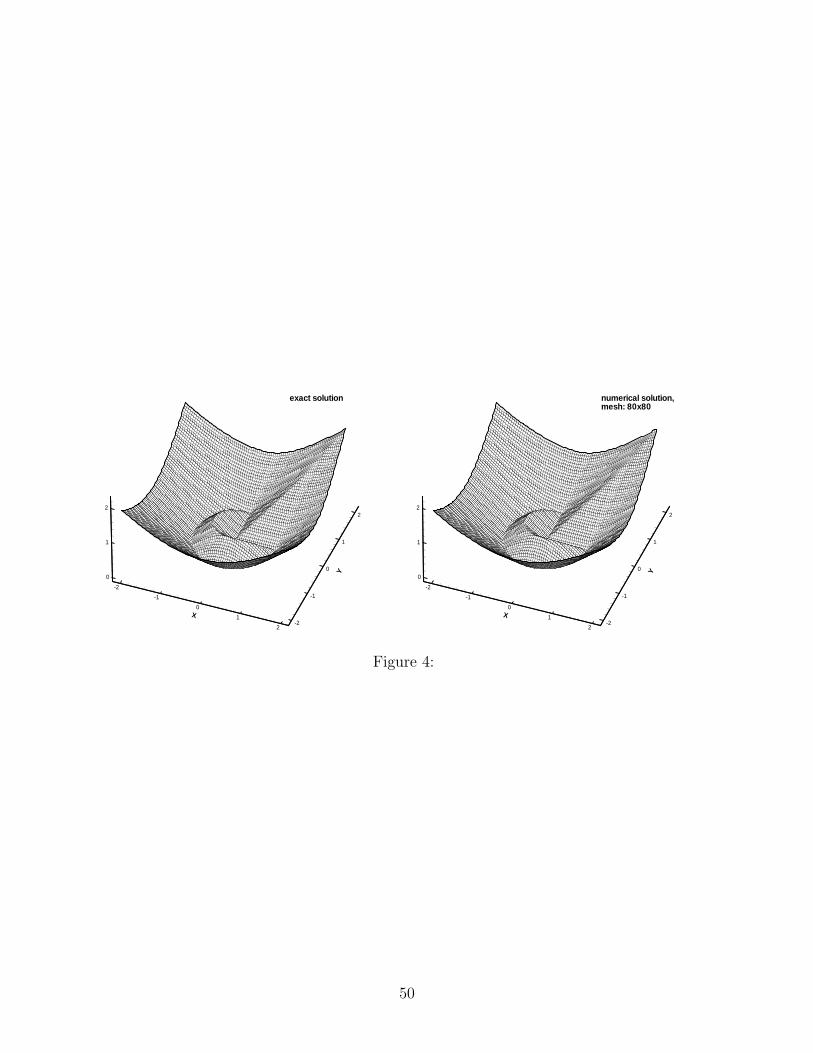
Example 5. Eikonal equation (2.2) with f(x, y) = 1. The Godunov Hamiltonian is

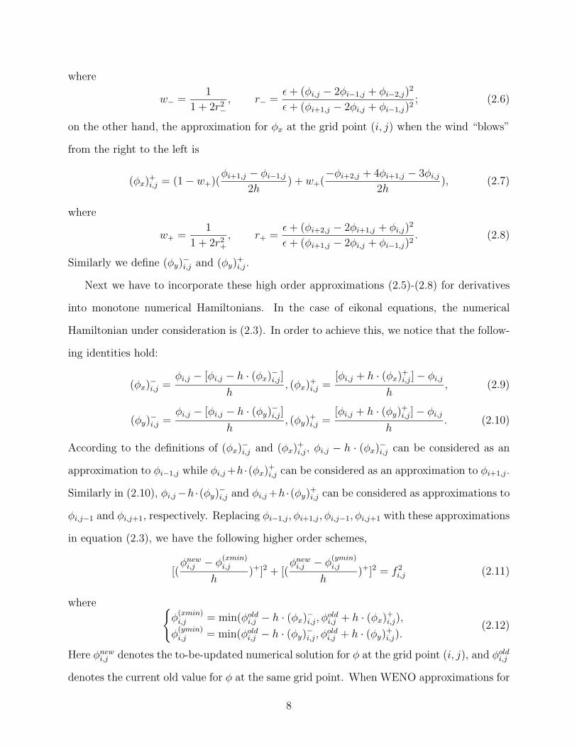
used. The computational domain Ω = [−2, 2] × [−2, 2], and Γ is a sector of three quarters

of a circle shown in Figure 3. So the exact solution is the distance function to the sector

Γ. Singularities at two corners in Γ give rise to different scenarios in different regions,

18

which include both shocks and rarefaction waves. In Figure 3, we illustrate the shocks by a

boldfaced solid line and three rarefaction wave regions with letter(s) “R” or “Rarefaction”;

the solution is smooth in other regions. During the mesh refinement, we fix the number of

grid points when we initialize the domain. Errors and convergence rates are presented in

Table 10. We only list results for L1 errors. The third order accuracy is obtained in the

regions where the solution is smooth. Moreover, we still obtain the second order accuracy in

the whole computational domain. The accuracy in the rarefaction wave region is consistent

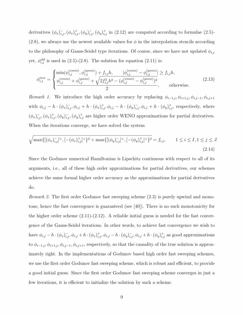
with the results in Example 4. We also plot the 3-D pictures of the exact solution and

numerical solution with an 80× 80 mesh in Figure 4; the sharp shock transition is apparent.

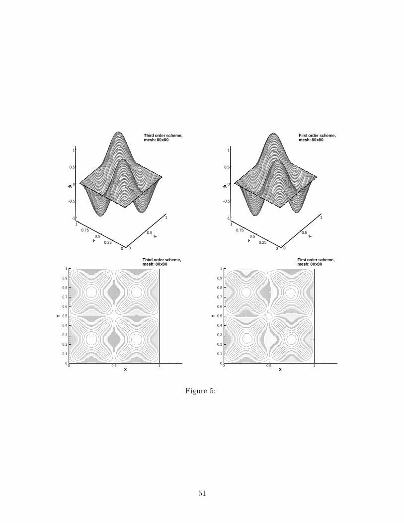
Example 6 (shape-from-shading). Eikonal equation (2.2) with

f(x, y) = 2π√

[cos(2πx) sin(2πy)]2 + [sin(2πx) cos(2πy)]2. (3.6)

Γ = (14, 1

4), (3

4, 3

4), (1

4, 3

4), (3

4, 1

4), (1

2, 1

2), consisting of five isolated points. The computational

domain Ω = [0, 1] × [0, 1]. φ(x, y) = 0 is prescribed at the boundary of the unit square.

The solution for this problem is the shape function, which has the brightness I(x, y) =

1/√

1 + f(x, y)2 under vertical lighting. See [31] for details. In [14], high order time marching

WENO schemes are used to calculate the solution for this problem. We apply both high

order Godunov based and Lax-Friedrichs based fast sweeping schemes to the following two

cases.

Case 1.

g(1

4,1

4) = g(

3

4,3

4) = 1, g(

1

4,3

4) = g(

3

4,1

4) = −1, g(

1

2,1

2) = 0.

The exact solution for this case is

φ(x, y) = sin(2πx) sin(2πy),

a smooth function.

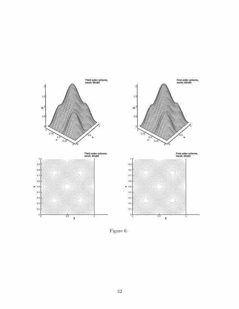
Case 2.

g(1

4,1

4) = g(

3

4,3

4) = g(

1

4,3

4) = g(

3

4,1

4) = 1, g(

1

2,1

2) = 2.

19

The exact solution for this case is

φ(x, y) =

max(| sin(2πx) sin(2πy)|, 1 + cos(2πx) cos(2πy)),

if |x+ y − 1| < 12

and |x− y| < 12;

| sin(2πx) sin(2πy)|, otherwise;

this solution is not smooth.

Errors, convergence rates and iteration numbers are reported in Table 11 and Table 12

for both Godunov and Lax-Friedrichs sweeping methods, respectively. Both methods yield

fully third order accuracy in the case of smooth solutions (Case 1). Since the exact solution

in Case 2 is not smooth, globally numerical errors indicate that the convergence order is

higher than the second order, which is consistent with the results in the examples shown

above. In terms of the iteration numbers shown in Table 11 and Table 12, the high order

Godunov fast sweeping method needs fewer iterations than the high order Lax-Friedrichs

fast sweeping method does. Figure 5 and Figure 6 illustrate three-dimensional pictures and

contour plots for numerical solutions of these two cases on the 80×80 mesh; these numerical

solutions are from both the third order Godunov scheme and the first order Godunov fast

sweeping method. Obviously, the high order method achieves much higher accuracy and

resolution than the first order scheme does on the same mesh. Figures by the Lax-Friedrichs

third order fast sweeping schemes are very similar to those by the Godunov Hamiltonian,

hence they are omitted to save space.

Remark 9. Using this example, we compared our third order fast sweeping method with

the time marching approach in [14], based on both Godunov and Lax-Friedrichs numerical

Hamiltonians, and the results are reported in Table 13. For the time marching approach,

we use the third order WENO in spatial direction [14] and a third order TVD Runge-Kutta

scheme [36] in time direction, and the CFL number is taken to be 0.6 as in [14]. The initial

guesses of the time marching method are totally the same as our third order fast sweeping

method; i.e., for the Godunov numerical Hamiltonian, they are generated by the first order

Godunov sweeping method; for the Lax-Friedrichs numerical Hamiltonian, the initial guesses

are just big values. The convergence criteria of both methods are the same too. In Table 13,

20

one iteration count of the time-marching approach includes three stages of the third order

TVD Runge-Kutta scheme, and one iteration count of the fast sweeping method includes

four alternating sweepings. For this example, the third order fast sweeping method with

the Godunov numerical Hamiltonian is about three times faster than the third order time-

marching approach on a 80 × 80 mesh. When the mesh is refined, the advantage of our

fast sweeping algorithm with the Godunov numerical Hamiltonian becomes more significant

due to the upwind property of the Godunov numerical Hamiltonian, and it is about eight

times faster than the third order time-marching approach on a 640×640 mesh. For the Lax-

Friedrichs numerical Hamiltonian, the third order fast sweeping method is about six times

faster than the third order time-marching approach for all mesh sizes. So our method is

much more efficient than the time-marching approach, for both Godunov and Lax-Friedrichs

numerical Hamiltonians.

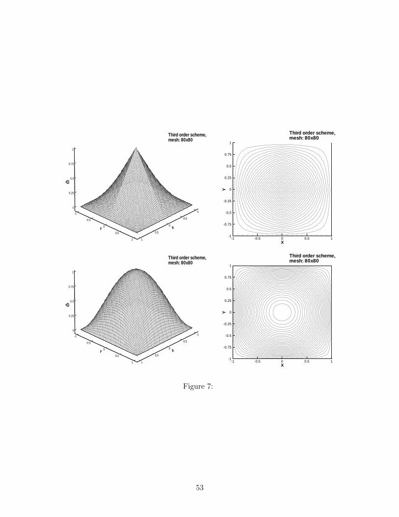
Example 7 (shape-from-shading). Eikonal equation (2.2) with

case (a): f(x, y) =√

(1 − |x|)2 + (1 − |y|)2; (3.7)

case (b): f(x, y) = 2√

y2(1 − x2)2 + x2(1 − y2)2. (3.8)

The computational domain Ω = [−1, 1] × [−1, 1]. φ(x, y) = 0 is prescribed at the boundary

of the square for both cases. Additional boundary condition φ(0, 0) = 1 is prescribed for

case (b). The exact solutions for these two cases are

case (a): φ(x, y) = (1 − |x|)(1 − |y|); (3.9)

case (b): φ(x, y) = (1 − x2)(1 − y2). (3.10)

In [13], a time-marching discontinuous Galerkin method is used to compute the solution

for these two cases. We apply our high order Godunov fast sweeping method to these

problems. Because the exact solution of case (a) is a piecewise bi-linear polynomial and

the exact solution of case (b) is a bi-quadratic polynomial, the numerical solutions by the

third order scheme are accurate up to round-off errors. Table 14 indicates that the errors for

both cases are round-off errors, and the iteration numbers in Table 14 demonstrate the fast

21

convergence of the scheme, which is again much faster than the time marching results. The

three-dimensional pictures and contour plots for the numerical solution of both cases on an

80 × 80 mesh are presented in Figure 7.

Example 8 (Travel-time problem in elastic wave propagation). The quasi-P and

the quasi-SV slowness surfaces are defined by the quadratic equation [26]:

c1φ4x + c2φ

2xφ

2y + c3φ

4y + c4φ

2x + c5φ

2y + 1 = 0, (3.11)

where

c1 = a11a44, c2 = a11a33 + a244 − (a13 + a44)

2, c3 = a33a44, c4 = −(a11 + a44), c5 = −(a33 + a44).

Here aijs are given elastic parameters. The corresponding quasi-P wave eikonal equation is

√

−1

2(c4φ2

x + c5φ2y) +

√

1

4(c4φ2

x + c5φ2y)

2 − (c1φ4x + c2φ2

xφ2y + c3φ4

y) = 1, (3.12)

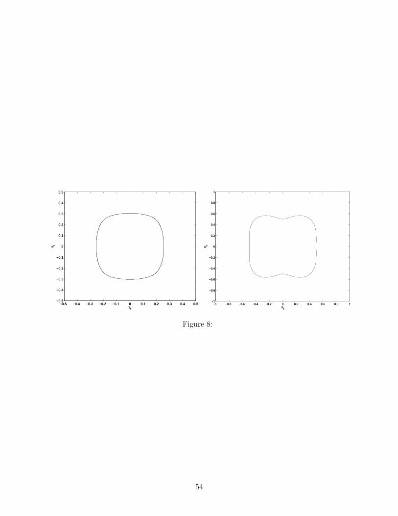
which is a convex Hamilton-Jacobi equation. The elastic parameters are taken to be

a11 = 15.0638, a33 = 10.8373, a13 = 1.6381, a44 = 3.1258

in the numerical example to be shown; Figure 8 shows the corresponding convex slowness

surface in the gradient component.

The corresponding quasi-SV wave eikonal equation is√

−1

2(c4φ2

x + c5φ2y) −

√

1

4(c4φ2

x + c5φ2y)

2 − (c1φ4x + c2φ2

xφ2y + c3φ4

y) = 1, (3.13)

which is a non-convex H-J equation. The elastic parameters are taken to be

a11 = 15.90, a33 = 6.21, a13 = 4.82, a44 = 4.00

in the numerical example to be shown; Figure 8 shows the corresponding non-convex slowness

surface in the gradient component.

The computational domain is [−1, 1]×[−1, 1], and Γ = (0, 0). Initial values are assigned

in a box with length 0.3 which includes the source point. Because both Hamiltonians are

22

pretty complicated, it is troublesome to apply the Godunov Hamiltonian to these examples.

Thus we apply the third order Lax-Friedrichs fast sweeping method (2.20) to these problems.

Errors and convergence rates are listed in Table 15 for the quasi-P wave travel-time, which

is smooth in the whole domain except at the source point. In fact, since the slowness surface

is convex, the resulting point-source solution is a pure rarefaction wave. To initialize a fixed

box around the source point, we use a shooting method by solving a two-point boundary

value problem; see [27] for details. The third order accuracy is obtained.

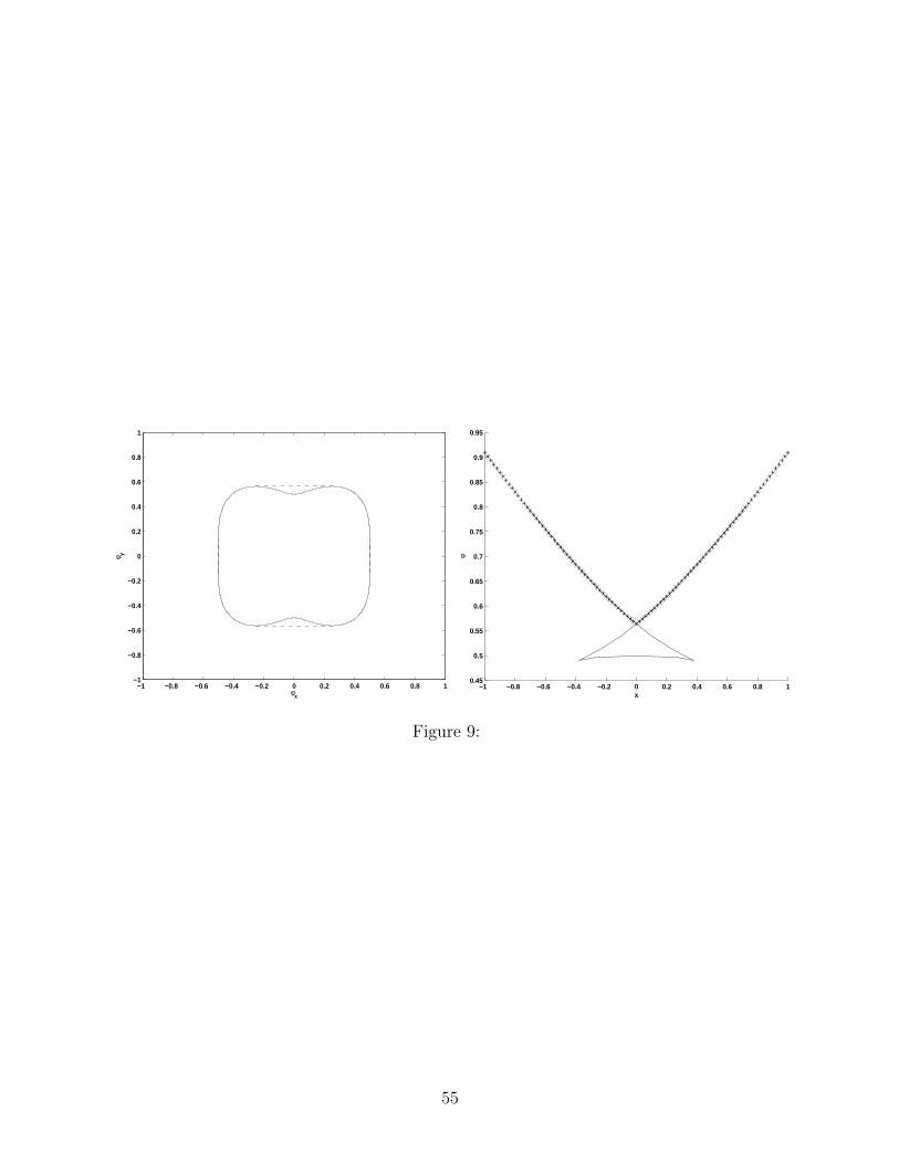
For the quasi-SV wave, the solution is smooth except along the lines x = 0 and y = 0

because of its non-convexity in the slowness space along the two axes. In this case, since

the outward normals of the slowness surface correspond to the ray directions in the physical

space according to the method of characteristics, we have so-called instantaneous singularities

along the lines x = 0 and y = 0 and the resulting travel-time field is multivalued; see the

solid lines in Figure 9. To pick out a unique, physically relevant solution, we convexify

the non-convex slowness surface first and then adapt a shooting method, similar to the one

used for quasi-P waves, to pick out a continuous solution; see the stars in Figure 9. This

construction agrees with a method based on the Huygens’s principle demonstrated in [30].

The shooting method is also used to initialize the traveltime field in a specified box around

the source point. Therefore, the point source problem for quasi-SV wave traveltime produces

both rarefaction and shock singularities.

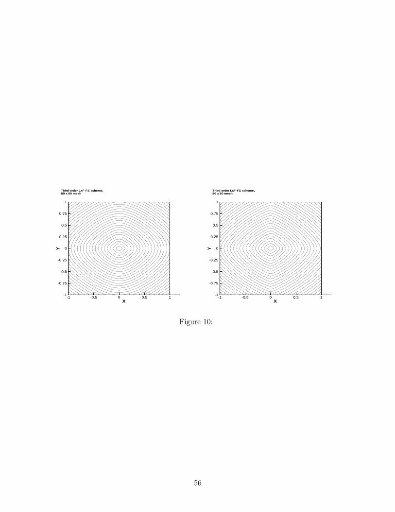
Table 16 illustrates that the third order accuracy is obtained in the smooth region of the

solution in both L1 and L∞ norms; however, in terms of the whole domain including the

shock wave region, the second order accuracy is obtained in the L1 norm and only the first

order accuracy is obtained in the L∞ norm. Overall, the third-order scheme achieves much

smaller errors than the first order scheme does, even in the shock wave region. The contour

plots of the solutions are shown in Figure 10. The quasi-SV solution agrees with the results

based on the Huygens’s principle shown in [30].

23

4 Concluding remarks

We have developed high order fast sweeping methods for static Hamilton-Jacobi equations

on rectangular meshes. A general procedure is given to incorporate the high order approx-

imations into monotone numerical Hamiltonians so that the first order sweeping schemes

can be extended to high order schemes. Extensive numerical examples demonstrate that the

high order methods yield higher order accuracy in the smooth region of the solution, higher

resolution for the singularities of derivatives, and fast convergence to viscosity solutions of

the Hamilton-Jacobi equations.

References

[1] R. Abgrall, Numerical discretization of the first-order Hamilton-Jacobi equation on tri-

angular meshes, Communications on Pure and Applied Mathematics, 49 (1996), 1339–

1373.

[2] S. Augoula and R. Abgrall, High order numerical discretization for Hamilton-Jacobi

equations on triangular meshes, Journal of Scientific Computing, 15 (2000), 197–229.

[3] M. Boue and P. Dupuis, Markov chain approximations for deterministic control problems

with affine dynamics and quadratic cost in the control, SIAM Journal on Numerical

Analysis, 36 (1999), 667–695.

[4] S. Bryson and D. Levy, High-order central WENO schemes for multidimensional

Hamilton-Jacobi equations, SIAM Journal on Numerical Analysis, 41 (2003), 1339-1369.

[5] T. Barth and J. Sethian, Numerical schemes for the Hamilton-Jacobi and level set

equations on triangulated domains, Journal of Computational Physics, 145 (1998), 1–40.

[6] T. Cecil, J. Qian and S. Osher, Numerical methods for high dimensional Hamilton-

Jacobi equations using radial basis functions, Journal of Computational Physics, 196

(2004), 327-347.

24

[7] M . G. Crandall and P. L. Lions, Viscosity solutions of Hamilton-Jacobi equations,

Trans. Amer. Math. Soc., 277 (1983), 1-42.

[8] J. Dellinger and W. W. Symes, Anisotropic finite-difference traveltimes using a

Hamilton-Jacobi solver, 67th Ann. Internat. Mtg., Soc. Expl. Geophys., Expanded Ab-

stracts, 1997, 1786-1789.

[9] M. Falcone and R. Ferretti, Discrete time high-order schemes for viscosity solutions of

Hamilton-Jacobi-Bellman equations, Numer. Math., 67 (1994), 315-344.

[10] M. Falcone and R. Ferretti, Semi-Lagrangian schemes for Hamilton-Jacobi equations,

discrete representation formulae and Godunov methods, Journal of Computational

Physics, 175 (2002), 559–575.

[11] S. Gray and W. May, Kirchhoff migration using eikonal equation travel-times, Geo-

physics, 59 (1994), 810-817.

[12] J. Helmsen, E. Puckett, P. Colella and M. Dorr, Two new methods for simulating pho-

tolithography development in 3d, Proc. SPIE, 1996, 2726:253-261.

[13] C. Hu and C.-W. Shu, A discontinuous Galerkin finite element method for Hamilton-

Jacobi equations, SIAM Journal on Scientific Computing, 20 (1999), 666-690.

[14] G.-S. Jiang and D. Peng, Weighted ENO Schemes for Hamilton-Jacobi equations, SIAM

Journal on Scientific Computing, 21 (2000), 2126–2143.

[15] G.-S. Jiang and C.-W. Shu, Efficient implementation of weighted ENO schemes, Journal

of Computational Physics, 126 (1996), 202–228.

[16] S. Jin and Z. Xin, Numerical passage from systems of conservation laws to Hamilton-

Jacobi equations and relaxation schemes, SIAM Journal on Numerical Analysis, 35

(1998), 2385–2404.

25

[17] S. Kim and R. Cook, 3D traveltime computation using second-order ENO scheme, Geo-

phys. 64 (1999), 1867-1876.

[18] C.Y. Kao, S. Osher and J. Qian, Lax-Friedrichs sweeping scheme for static Hamilton-

Jacobi equations, Journal of Computational Physics, 196 (2004), 367-391.

[19] C.Y. Kao, S. Osher and Y.H. Tsai, Fast Sweeping Methods for Hamilton-Jacobi Equa-

tions, to appear in SINUM.

[20] C.-T. Lin and E. Tadmor, High-resolution non-oscillatory central schemes for approx-

imate Hamilton-Jacobi equations, SIAM Journal on Scientific Computing, 21 (2000),

2163–2186.

[21] C.-T. Lin and E. Tadmor, L1-stability and error estimates for approximate Hamilton-

Jacobi solutions, Numer. Math., 87 (2001), 701–735.

[22] S. Osher, A level set formulation for the solution of the Dirichlet problem for Hamilton-

Jacobi equations, SIAM J. Math. Anal. 24 (1993), 1145-1152.

[23] S. Osher and J. Sethian, Fronts propagating with curvature dependent speed: algorithms

based on Hamilton-Jacobi formulations, Journal of Computational Physics, 79 (1988),

12–49.

[24] S. Osher and C.-W. Shu, High-order essentially nonoscillatory schemes for Hamilton-

Jacobi equations, SIAM Journal on Numerical Analysis, 28 (1991), 907–922.

[25] D. Peng, S. Osher, B. Merriman, H.-K. Zhao and M. Rang, A PDE-based fast local level

set method, Journal of Computational Physics, 155 (1999), 410–438.

[26] J. Qian, L.T. Cheng and S. Osher, A level set based Eulerian approach for anisotropic

wave propagations, Wave Motion, 37 (2003), 365-379.

[27] J. Qian and W. W. Symes, Paraxial eikonal solvers for anisotropic quasi-P travel times,

Journal of Computational Physics, 174 (2001), 256-278.

26

[28] J. Qian and W. W. Symes, Finite-difference quasi-P traveltimes for anisotropic media,

Geophysics, 67 (2002), 147-155.

[29] J. Qian and W. W. Symes, An adaptive finite-difference method for traveltime and

amplitude, Geophysics, 67 (2002), 166-176.

[30] F. Qin and G. T. Schuster, First-arrival traveltime calculation for anisotropic media,

Geophysics, 58 (1993), 1349-1358.

[31] E. Rouy and A. Tourin, A viscosity solutions approach to shape-from-shading, SIAM

Journal on Numerical Analysis, 29 (1992), 867–884.

[32] J. A. Sethian, A fast marching level set method for monotonically advancing fronts,

Proc. Nat. Acad. Sci., 93 (1996), 1591–1595.

[33] J. A. Sethian and A. Vladimirsky, Ordered upwind methods for static Hamilton-Jacobi

equations, Proc. Natl. Acad. Sci., 98(2001), 11069-11074.

[34] J.A. Sethian and A. Vladimirsky, Ordered upwind methods for static Hamilton-Jacobi

equations: theory and algorithms, SIAM Journal on Numerical Analysis, 41 (2003),

325-363.

[35] Chi-Wang Shu, High order numerical methods for time dependent Hamilton-Jacobi equa-

tions, WSPC/Lecture Notes Series, 2004.

[36] C.-W. Shu and S. Osher, Efficient Implementation of Essentially Non-Oscillatory Shock-

Capturing Schemes, Journal of Computational Physics, 77 (1988), 439-471.

[37] Y.-H. R. Tsai, L.-T. Cheng, S. Osher and H.-K. Zhao, Fast sweeping algorithms for a

class of Hamilton-Jacobi equations, SIAM Journal on Numerical Analysis, 41 (2003),

673-694.

[38] J.N. Tsitsiklis, Efficient algorithms for globally optimal trajectories, IEEE Transactions

on Automatic Control, 40 (1995), 1528-1538.

27

[39] Y.-T. Zhang and C.-W. Shu, High order WENO schemes for Hamilton-Jacobi equations

on triangular meshes, SIAM Journal on Scientific Computing, 24 (2003), 1005-1030.

[40] H. Zhao, A fast sweeping method for Eikonal equations, Math. Comp., 74 (2004), 603-

627

[41] H. Zhao, S. Osher, B. Merriman and M. Kang, Implicit and non-parametric shape

reconstruction from unorganized points using variational level set method, Computer

Vision and Image Understanding, 80 (2000), 295–319.

28

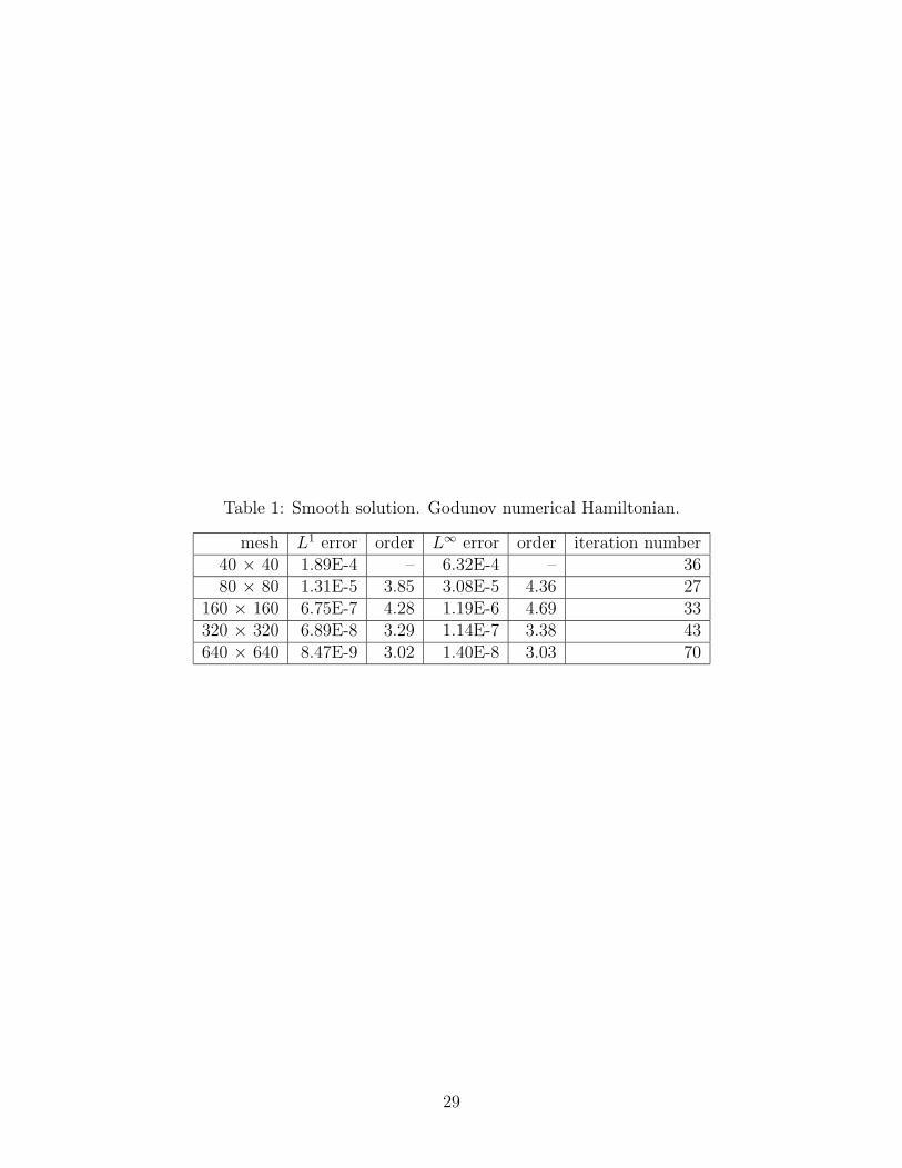
Table 1: Smooth solution. Godunov numerical Hamiltonian.

mesh L1 error order L∞ error order iteration number40 × 40 1.89E-4 – 6.32E-4 – 3680 × 80 1.31E-5 3.85 3.08E-5 4.36 27

160 × 160 6.75E-7 4.28 1.19E-6 4.69 33320 × 320 6.89E-8 3.29 1.14E-7 3.38 43640 × 640 8.47E-9 3.02 1.40E-8 3.03 70

29

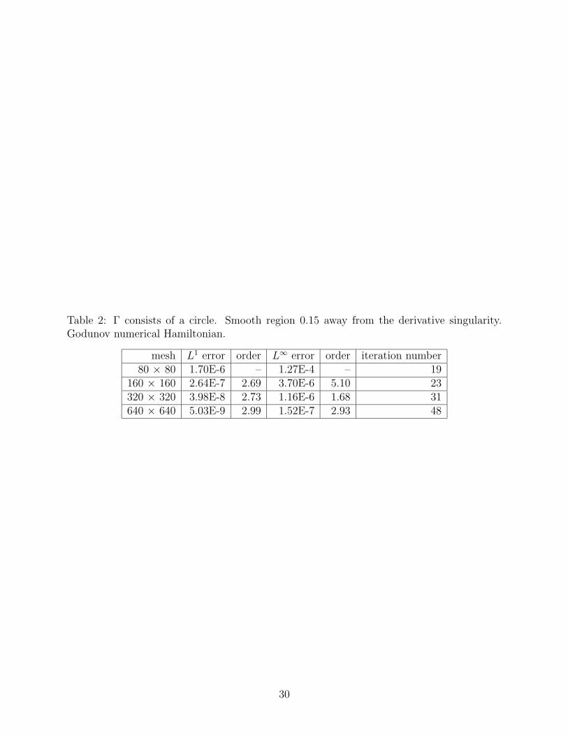
Table 2: Γ consists of a circle. Smooth region 0.15 away from the derivative singularity.Godunov numerical Hamiltonian.

mesh L1 error order L∞ error order iteration number80 × 80 1.70E-6 – 1.27E-4 – 19

160 × 160 2.64E-7 2.69 3.70E-6 5.10 23320 × 320 3.98E-8 2.73 1.16E-6 1.68 31640 × 640 5.03E-9 2.99 1.52E-7 2.93 48

30

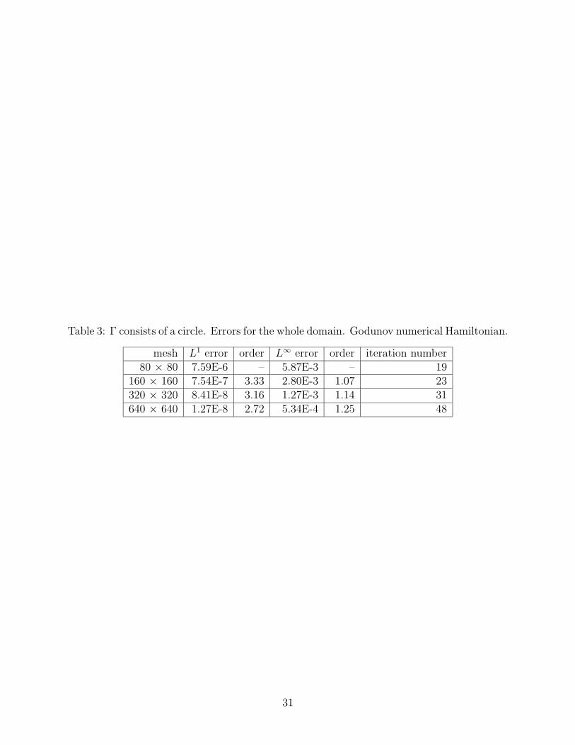
Table 3: Γ consists of a circle. Errors for the whole domain. Godunov numerical Hamiltonian.


160 × 160 7.54E-7 3.33 2.80E-3 1.07 23320 × 320 8.41E-8 3.16 1.27E-3 1.14 31640 × 640 1.27E-8 2.72 5.34E-4 1.25 48

31

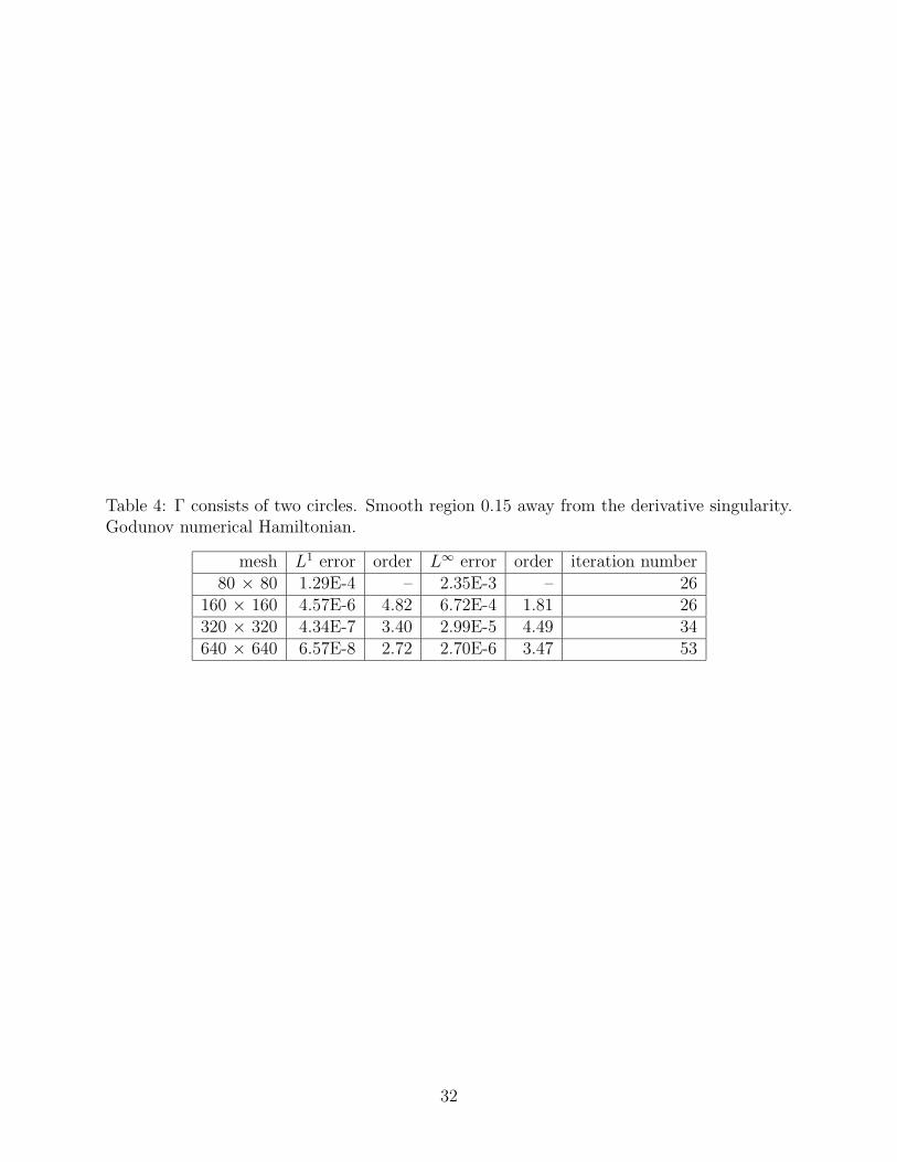
Table 4: Γ consists of two circles. Smooth region 0.15 away from the derivative singularity.Godunov numerical Hamiltonian.


160 × 160 4.57E-6 4.82 6.72E-4 1.81 26320 × 320 4.34E-7 3.40 2.99E-5 4.49 34640 × 640 6.57E-8 2.72 2.70E-6 3.47 53

32

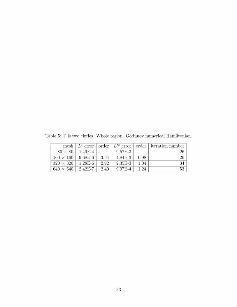
Table 5: Γ is two circles. Whole region. Godunov numerical Hamiltonian.


160 × 160 9.68E-6 3.94 4.84E-3 0.98 26320 × 320 1.28E-6 2.92 2.35E-3 1.04 34640 × 640 2.42E-7 2.40 9.97E-4 1.24 53

33

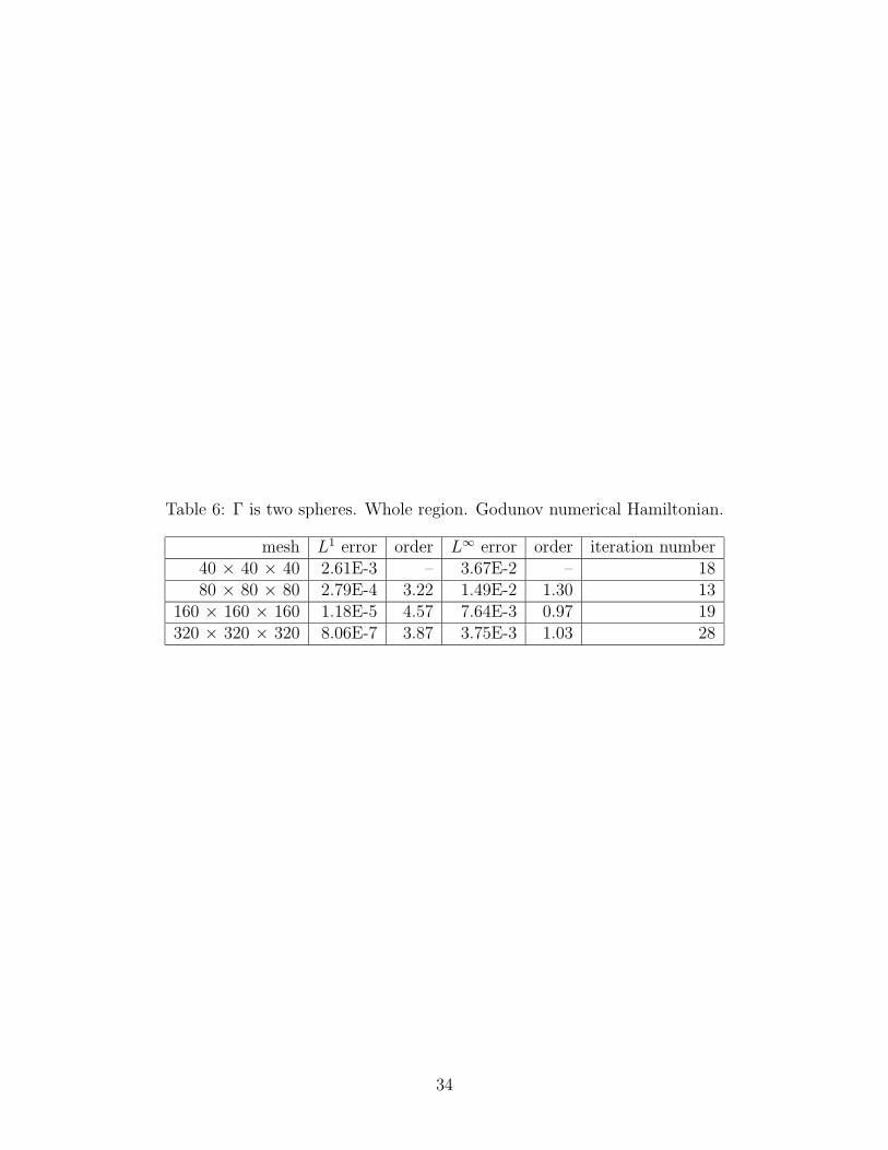
Table 6: Γ is two spheres. Whole region. Godunov numerical Hamiltonian.

mesh L1 error order L∞ error order iteration number40 × 40 × 40 2.61E-3 – 3.67E-2 – 1880 × 80 × 80 2.79E-4 3.22 1.49E-2 1.30 13

160 × 160 × 160 1.18E-5 4.57 7.64E-3 0.97 19320 × 320 × 320 8.06E-7 3.87 3.75E-3 1.03 28

34

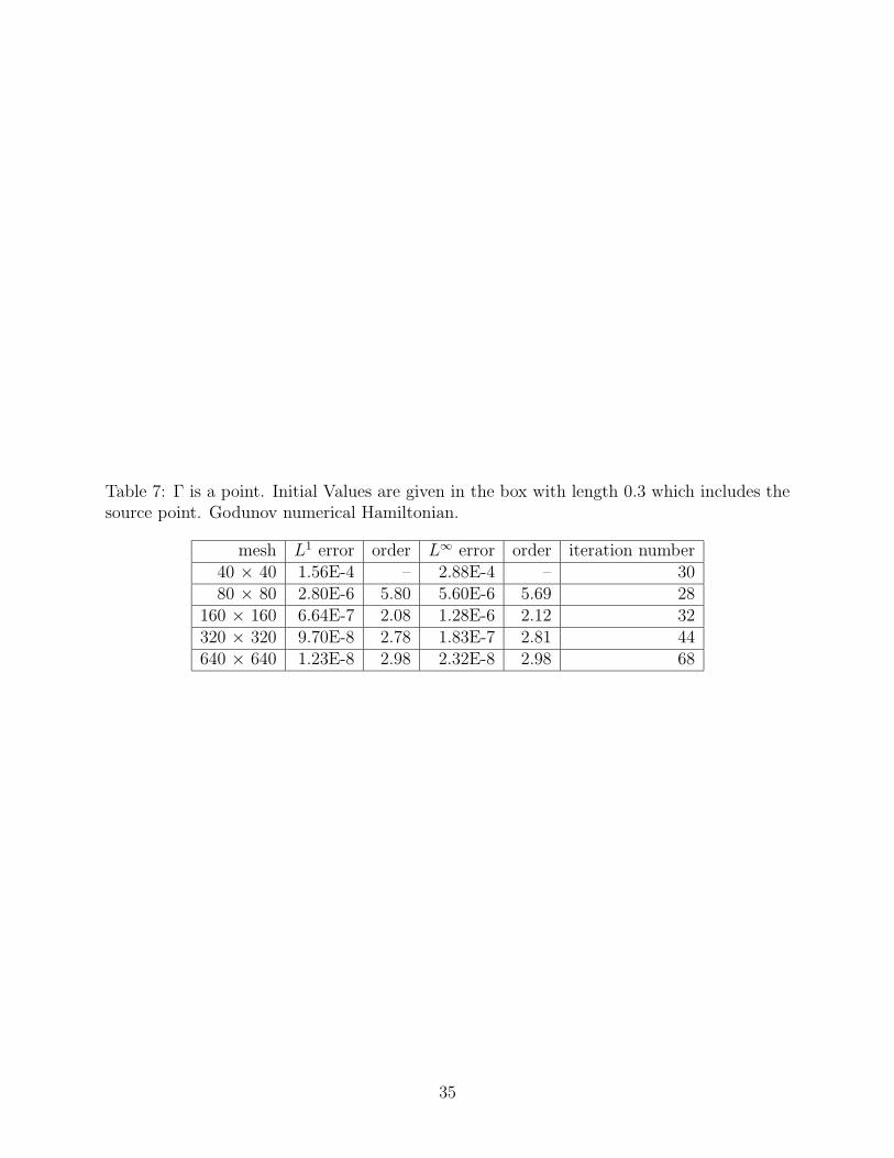
Table 7: Γ is a point. Initial Values are given in the box with length 0.3 which includes thesource point. Godunov numerical Hamiltonian.


160 × 160 6.64E-7 2.08 1.28E-6 2.12 32320 × 320 9.70E-8 2.78 1.83E-7 2.81 44640 × 640 1.23E-8 2.98 2.32E-8 2.98 68

35

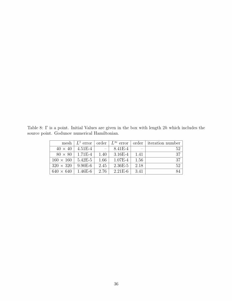
Table 8: Γ is a point. Initial Values are given in the box with length 2h which includes thesource point. Godunov numerical Hamiltonian.


160 × 160 5.42E-5 1.66 1.07E-4 1.56 37320 × 320 9.90E-6 2.45 2.36E-5 2.18 52640 × 640 1.46E-6 2.76 2.21E-6 3.41 84

36

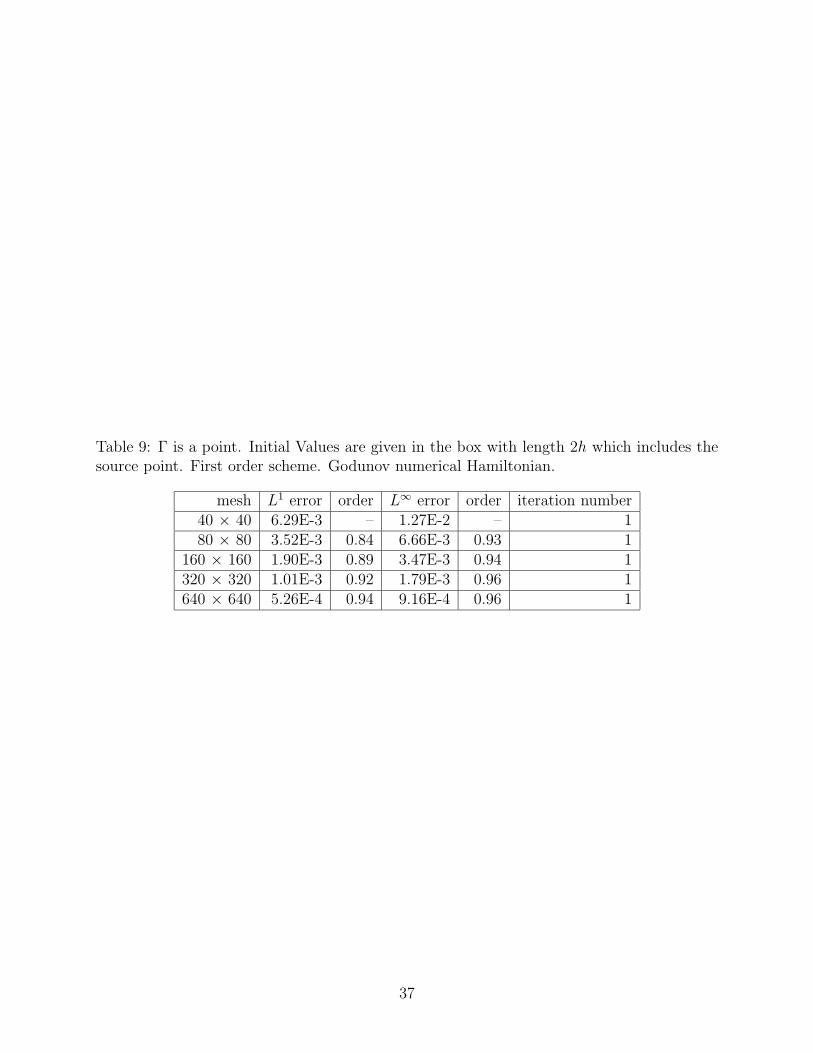
Table 9: Γ is a point. Initial Values are given in the box with length 2h which includes thesource point. First order scheme. Godunov numerical Hamiltonian.


160 × 160 1.90E-3 0.89 3.47E-3 0.94 1320 × 320 1.01E-3 0.92 1.79E-3 0.96 1640 × 640 5.26E-4 0.94 9.16E-4 0.96 1

37

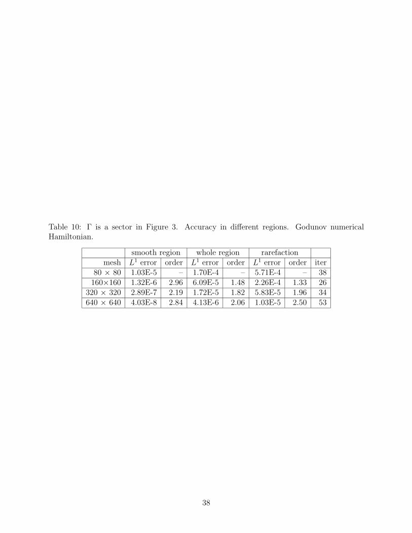
Table 10: Γ is a sector in Figure 3. Accuracy in different regions. Godunov numericalHamiltonian.

smooth region whole region rarefactionmesh L1 error order L1 error order L1 error order iter

80 × 80 1.03E-5 – 1.70E-4 – 5.71E-4 – 38160×160 1.32E-6 2.96 6.09E-5 1.48 2.26E-4 1.33 26

320 × 320 2.89E-7 2.19 1.72E-5 1.82 5.83E-5 1.96 34640 × 640 4.03E-8 2.84 4.13E-6 2.06 1.03E-5 2.50 53

38

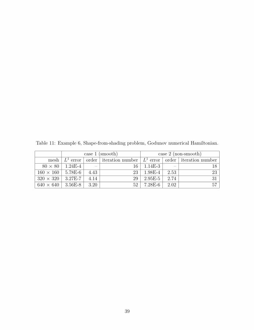
Table 11: Example 6, Shape-from-shading problem, Godunov numerical Hamiltonian.

case 1 (smooth) case 2 (non-smooth)mesh L1 error order iteration number L1 error order iteration number

80 × 80 1.24E-4 – 16 1.14E-3 – 18160 × 160 5.78E-6 4.43 23 1.98E-4 2.53 23320 × 320 3.27E-7 4.14 29 2.95E-5 2.74 31640 × 640 3.56E-8 3.20 52 7.28E-6 2.02 57

39

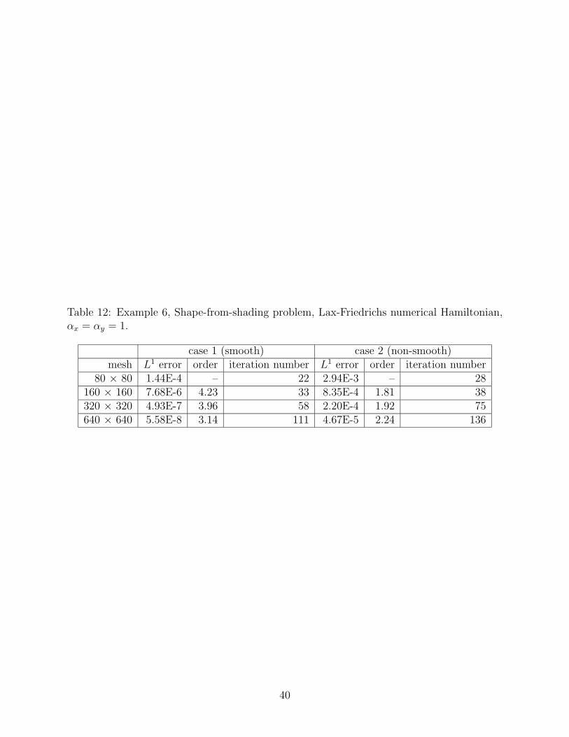
Table 12: Example 6, Shape-from-shading problem, Lax-Friedrichs numerical Hamiltonian,αx = αy = 1.

case 1 (smooth) case 2 (non-smooth)mesh L1 error order iteration number L1 error order iteration number

80 × 80 1.44E-4 – 22 2.94E-3 – 28160 × 160 7.68E-6 4.23 33 8.35E-4 1.81 38320 × 320 4.93E-7 3.96 58 2.20E-4 1.92 75640 × 640 5.58E-8 3.14 111 4.67E-5 2.24 136

40

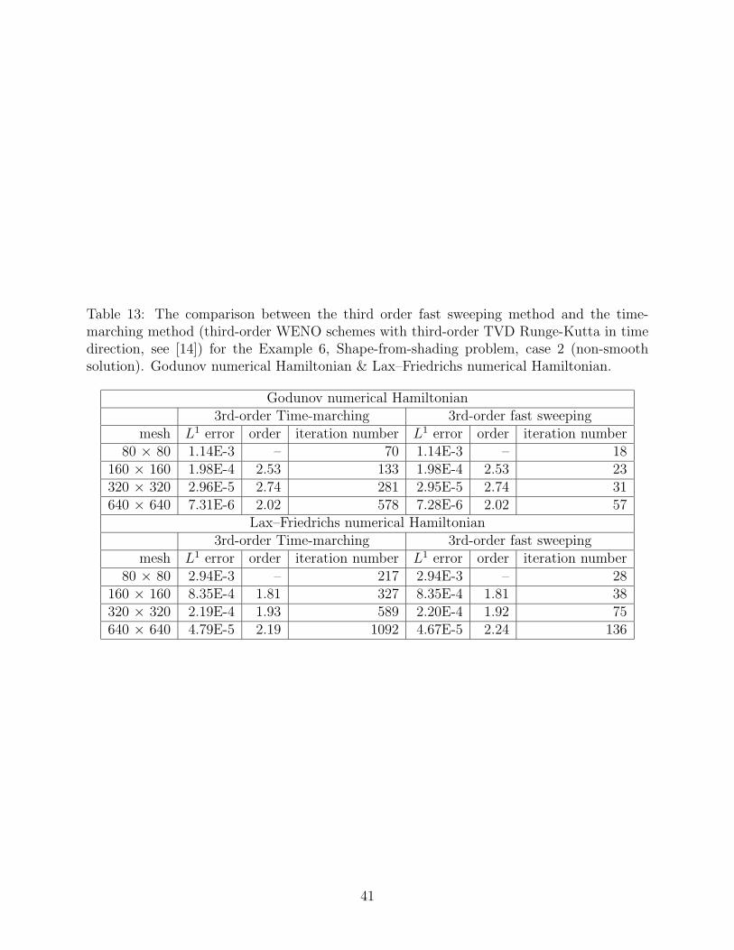
Table 13: The comparison between the third order fast sweeping method and the time-marching method (third-order WENO schemes with third-order TVD Runge-Kutta in timedirection, see [14]) for the Example 6, Shape-from-shading problem, case 2 (non-smoothsolution). Godunov numerical Hamiltonian & Lax–Friedrichs numerical Hamiltonian.

Godunov numerical Hamiltonian3rd-order Time-marching 3rd-order fast sweeping

mesh L1 error order iteration number L1 error order iteration number80 × 80 1.14E-3 – 70 1.14E-3 – 18

160 × 160 1.98E-4 2.53 133 1.98E-4 2.53 23320 × 320 2.96E-5 2.74 281 2.95E-5 2.74 31640 × 640 7.31E-6 2.02 578 7.28E-6 2.02 57

Lax–Friedrichs numerical Hamiltonian3rd-order Time-marching 3rd-order fast sweeping

mesh L1 error order iteration number L1 error order iteration number80 × 80 2.94E-3 – 217 2.94E-3 – 28

160 × 160 8.35E-4 1.81 327 8.35E-4 1.81 38320 × 320 2.19E-4 1.93 589 2.20E-4 1.92 75640 × 640 4.79E-5 2.19 1092 4.67E-5 2.24 136

41

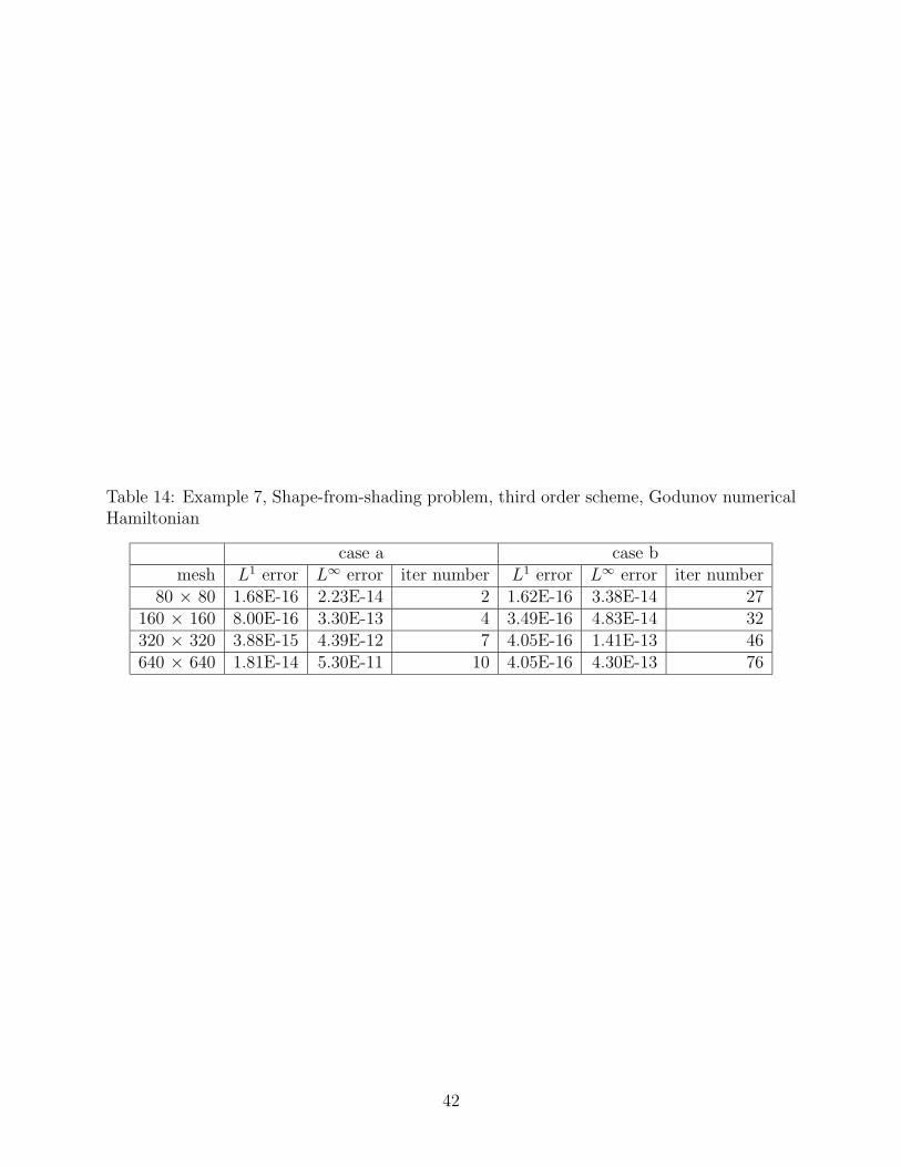
Table 14: Example 7, Shape-from-shading problem, third order scheme, Godunov numericalHamiltonian

case a case bmesh L1 error L∞ error iter number L1 error L∞ error iter number

80 × 80 1.68E-16 2.23E-14 2 1.62E-16 3.38E-14 27160 × 160 8.00E-16 3.30E-13 4 3.49E-16 4.83E-14 32320 × 320 3.88E-15 4.39E-12 7 4.05E-16 1.41E-13 46640 × 640 1.81E-14 5.30E-11 10 4.05E-16 4.30E-13 76

42

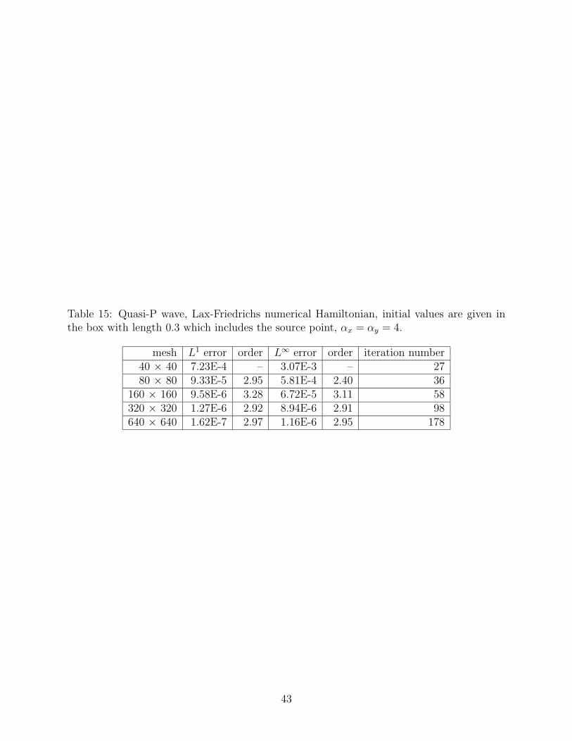
Table 15: Quasi-P wave, Lax-Friedrichs numerical Hamiltonian, initial values are given inthe box with length 0.3 which includes the source point, αx = αy = 4.


160 × 160 9.58E-6 3.28 6.72E-5 3.11 58320 × 320 1.27E-6 2.92 8.94E-6 2.91 98640 × 640 1.62E-7 2.97 1.16E-6 2.95 178

43

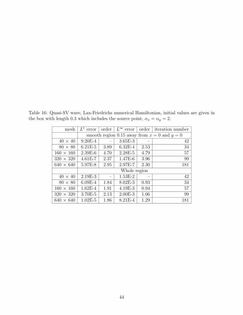
Table 16: Quasi-SV wave, Lax-Friedrichs numerical Hamiltonian, initial values are given inthe box with length 0.3 which includes the source point, αx = αy = 2.

mesh L1 error order L∞ error order iteration numbersmooth region 0.15 away from x = 0 and y = 0

40 × 40 9.20E-4 – 3.65E-3 – 4280 × 80 6.21E-5 3.89 6.32E-4 2.53 34

160 × 160 2.39E-6 4.70 2.28E-5 4.79 57320 × 320 4.61E-7 2.37 1.47E-6 3.96 99640 × 640 5.97E-8 2.95 2.97E-7 2.30 181

Whole region40 × 40 2.19E-3 – 1.53E-2 – 4280 × 80 6.09E-4 1.84 8.02E-3 0.93 34

160 × 160 1.62E-4 1.91 4.19E-3 0.94 57320 × 320 3.70E-5 2.13 2.00E-3 1.06 99640 × 640 1.02E-5 1.86 8.21E-4 1.29 181

44

Figure Captions

Figure 1: stencil of the third-order WENO scheme.

Figure 2: Two Spheres problem. Godunov numerical Hamiltonian. Top left: contour plot

for the whole surface; top right: a part of the interior region; bottom left: the contour plot

for φ = 0.5; bottom right: the contour plot for φ = 1.0. For the contour lines in the top two

pictures, there are 30 equally spaced of them from φ = 0.2 to φ = 4. Third order numerical

solution with 80 × 80 × 80 mesh.

Figure 3: Γ is a sector.

Figure 4: Distance to Γ. where Γ is a sector in Figure 3. Godunov numerical Hamilto-

nian. Left: exact solution; right: third order numerical solution with 80 × 80 mesh.

Figure 5: Example 6, shape-from-shading, case 1. Godunov numerical Hamiltonian. Left:

third order scheme; right: first order scheme; top: three-dimensional view; bottom: contour

lines, 30 equally spaced contour lines from φ = −1 to φ = 1.

Figure 6: Example 6, shape-from-shading, case 2. Godunov numerical Hamiltonian. Left:

third order scheme; right: first order scheme; top: three-dimensional view; bottom: contour

lines, 30 equally spaced contour lines from φ = 0 to φ = 2.

Figure 7: Example 7, shape-from-shading. Third order scheme, Godunov numerical Hamil-

tonian. Top left: three-dimensional view for case (a); bottom left: three-dimensional view

for case (b); top right: contour lines for case (a), 30 equally spaced contour lines from φ = 0

to φ = 1; bottom right: contour lines for case (b), 30 equally spaced contour lines from φ = 0

to φ = 1.

45

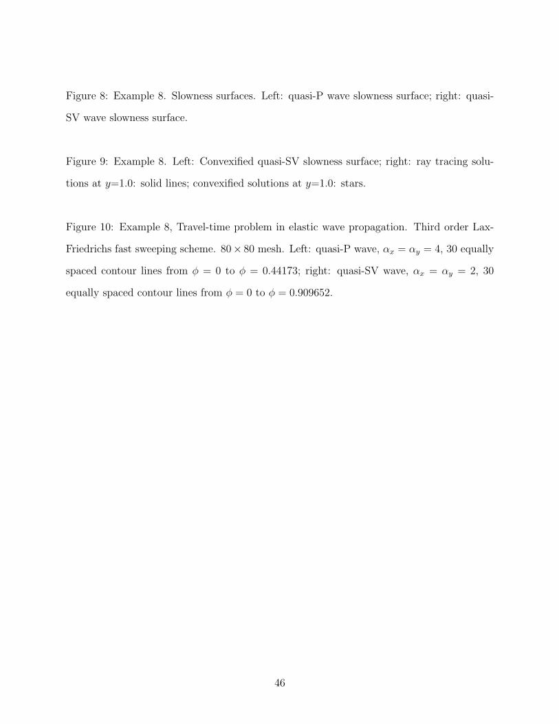
Figure 8: Example 8. Slowness surfaces. Left: quasi-P wave slowness surface; right: quasi-

SV wave slowness surface.

Figure 9: Example 8. Left: Convexified quasi-SV slowness surface; right: ray tracing solu-

tions at y=1.0: solid lines; convexified solutions at y=1.0: stars.

Figure 10: Example 8, Travel-time problem in elastic wave propagation. Third order Lax-

Friedrichs fast sweeping scheme. 80× 80 mesh. Left: quasi-P wave, αx = αy = 4, 30 equally

spaced contour lines from φ = 0 to φ = 0.44173; right: quasi-SV wave, αx = αy = 2, 30

equally spaced contour lines from φ = 0 to φ = 0.909652.

46

φx+-

i-2 i-1 i i+1 i+2

φx

Figure 1:

47

X

-2

0

2

Y

-2

0

2

Z

-2

0

2

Phi

4.003.873.743.613.483.343.213.082.952.822.692.562.432.302.172.031.901.771.641.511.381.251.120.990.860.720.590.460.330.20

80 x 80 x 80 mesh3rd-order Godunovfast-sweeping

X

-2

0

2

Y

-2

0

2

Z

-2

0

2

Phi

4.003.873.743.613.483.343.213.082.952.822.692.562.432.302.172.031.901.771.641.511.381.251.120.990.860.720.590.460.330.20

80 x 80 x 80 mesh3rd-order Godunovfast-sweeping

Interior of left picture

X

-20

2

Y

-2

0

2

Z

-2

0

2

Phi

4.003.873.743.613.483.343.213.082.952.822.692.562.432.302.172.031.901.771.641.511.381.251.120.990.860.720.590.460.330.20

80 x 80 x 80 mesh3rd-order Godunov fast-sweepingthe contour = 0.5 in 3D

X

-20

2

Y

-2

0

2

Z

-2

0

2

Phi

4.003.873.743.613.483.343.213.082.952.822.692.562.432.302.172.031.901.771.641.511.381.251.120.990.860.720.590.460.330.20

80 x 80 x 80 mesh3rd-order Godunov fast-sweepingthe contour = 1.0 in 3D

Figure 2:

48

ShockRarefaction

Rarefaction

R

Figure 3:

49

0

1

2

-2

-1

0

1

2

X-2

-1

0

1

2

Y

exact solution

0

1

2

-2

-1

0

1

2

X-2

-1

0

1

2

Y

numerical solution,mesh: 80x80

Figure 4:

50

-1

-0.5

0

0.5

1

φ

0

0.5

1

X

0

0.25

0.5

0.75

1

Y

Third order scheme,mesh: 80x80

-1

-0.5

0

0.5

1

φ

0

0.5

1

X

0

0.25

0.5

0.75

1

Y

First order scheme,mesh: 80x80

X

Y

0 0.5 10

0.1

0.2

0.3

0.4

0.5

0.6

0.7

0.8

0.9

1


X

Y

0 0.5 10

0.1

0.2

0.3

0.4

0.5

0.6

0.7

0.8

0.9

1


Figure 5:

51

0

0.5

1

1.5

2

φ

0

0.5

1

X

0

0.25

0.5

0.75

1

Y


0

0.5

1

1.5

2

φ

0

0.5

1

X

0

0.25

0.5

0.75

1

Y


X

Y

0 0.5 10

0.1

0.2

0.3

0.4

0.5

0.6

0.7

0.8

0.9

1


X

Y

0 0.5 10

0.1

0.2

0.3

0.4

0.5

0.6

0.7

0.8

0.9

1


Figure 6:

52

0

0.25

0.5

0.75

1

φ

-1

-0.5

0

0.5

1

X

-1

-0.5

0

0.5

1

Y


X

Y

-1 -0.5 0 0.5 1-1

-0.75

-0.5

-0.25

0

0.25

0.5

0.75

1


0

0.25

0.5

0.75

1

φ-1

-0.5

0

0.5

1

X

-1

-0.5

0

0.5

1

Y


X

Y

-1 -0.5 0 0.5 1-1

-0.75

-0.5

-0.25

0

0.25

0.5

0.75

1


Figure 7:

53

−0.5 −0.4 −0.3 −0.2 −0.1 0 0.1 0.2 0.3 0.4 0.5−0.5

−0.4

−0.3

−0.2

−0.1

0

0.1

0.2

0.3

0.4

0.5

φx

φ y

−1 −0.8 −0.6 −0.4 −0.2 0 0.2 0.4 0.6 0.8 1−1

−0.8

−0.6

−0.4

−0.2

0

0.2

0.4

0.6

0.8

1

φx

φ y

Figure 8:

54

−1 −0.8 −0.6 −0.4 −0.2 0 0.2 0.4 0.6 0.8 1−1

−0.8

−0.6

−0.4

−0.2

0

0.2

0.4

0.6

0.8

1

φx

φ y

−1 −0.8 −0.6 −0.4 −0.2 0 0.2 0.4 0.6 0.8 10.45

0.5

0.55

0.6

0.65

0.7

0.75

0.8

0.85

0.9

0.95

x

φ

Figure 9:

55

X

Y

-1 -0.5 0 0.5 1-1

-0.75

-0.5

-0.25

0

0.25

0.5

0.75

1

Third-order LxF-FS scheme,80 x 80 mesh

X

Y

-1 -0.5 0 0.5 1-1

-0.75

-0.5

-0.25

0

0.25

0.5

0.75

1

Third-order LxF-FS scheme,80 x 80 mesh

Figure 10:

56

Documents

High order fast sweeping methods for static Hamilton ...zhao/publication/mypapers/pdf/FS_high... · High order fast sweeping methods for static Hamilton-Jacobi equations ... (WENO)