Embed Size (px)
Citation preview

Automatic Control Laboratory, ETH Zürich!
Fast Model Predictive Control (MPC)"!
Manfred Morari!!with thanks to !Colin Jones, Paul Goulart, !Alex Domahidi, Stefan Richter!and many other collaborators!!
Automatic Control Laboratory, ETH Zürich!
Fast Model Predictive Control (MPC)"!
Manfred Morari!!with thanks to !Colin Jones, Paul Goulart, !Alex Domahidi, Stefan Richter!and many other collaborators!!

My first “encounter” with Keith….!
where
and where
L
(45)
-Ji, is equal to .X, with A,’, 4;. pl, T:, 9: replaced by A,z, 4f, p2. +*, 25:, - OS:, respectively.
Proof: The proof of Theorem 2 follows by carrying out exactly the same procedure as done in Theorem 1; the details are omitted.
Remark 5: Theorem 2 shows that the steady-state invertibility condi- tions for a system can be expressed solely in terms of a system’s steady-state parameters; this result is important in identifying compensa- tors for unknown systems [20].
Remark 6: It is to be noted that the computational effort required to test the condtions of Theorem 2 and solve for the gains (44) is signifi- cantly less than that required to test the conditions of Theorem 1 and solve for the gains (6). (7Ei.e., in the case of calculating (6) and (7), the computation time approximately varies as n3 max ( n , , n d 3 ; in the case of calculating (441, the computation time approximateIy vanes as r3p3 where p 2 max (4,’. i= l ; . . .p’; 4:. i = 1;..,p2), and r < n , p< max (n, ,nJ normally.
VI. CONCLUSIONS
The notion of steady-state invertibility of a system whch is basically concerned with the invertibility of a system under steady-state operating conditions (no transients) is considered in this short paper. Necessary and sufficient conditions that a system be steady-state invertible are obtained; in particular, it is shown that the steady-state invertibility condition can be expressed in terms of the system’s transfer function matrix of the system. It is shown that a system whch is minimum phase and which has at least the same number of inputs as outputs is always steady-state invertible. It is also shown that if there are at least the same number of inputs as outputs in the system, then the system is “almost always” steady-state invertible-if there are more outputs than inputs, then the system is “almost never” steady-state invertible. Application of these results is then made to the problem of finding a feedforward controller for a general system subject to measurable disturbances, so that the resultant controlled system is stable and has asymptotic regula- tion occurring.
IEEE TRANMCTIONS ON AUTOMATIC CONTROL, AUGUST 1976
REFERENCES
E. J. Davison, “Tbe feedforward, feedback and robust control of a general
Circuit and System Theory, O c t 1973. servomechanism proble-Part I,” presented at the 11th Ann. Allenon Conf.
M. Sain and J. L. Massey, “Invertibility of linear time-invariant dynamical sys- tems,” ZEEE T m . Auromot. Conrr., vol. AC-14, pp. 141-149, Apr. 1969. L. M. Silvermatl, ”Inversion of multivariable hear systems,” IEEE Tram. A u r o ~ . Conrr., vol. AC-14, pp. 27S276, June 1969.
Automar. Contr.. vol. AC-16, pp. 568-581, D e c 1971. A. S. Morse and W. M. Wonham, “Status of noninteracting control” ZEEE Tram
L. M. Silverman and H. J. Payne, “lnputdutput smctwe of linear systems with application to the decoupling problem,” SZAM J. Conrr., voL 9, pp. 199-233, 141. E. J. Davison, “The feedforward control of linear multivariable time-invarht systems” Aufomatica, vol. 9, pp. 561-573, 1973. F. G. Shinskey, Process-Conrrol Sysfem. New York: McGraw-Hill, I%?, ch. 8.
Addison-Wesley, 1969, pp. 91-100. L. A. Gould, Chemical Process Control: Theory and Applications. Reading, M A
H. W. Smith and E. J. Davison, “The design of industrial regulators Inte@al feedback and feedforward control,“ Proc. Zmr. €kc. Eng., vol. 110, no. 8, pp.
W. A Wolovich, ‘Static decoupling.” IEEE Tram. Aufomat. Conrr., voL AC-18. pp. 121C-1216, 1972.
536537, Oct. 1973. E. .I. Davison, “On the optimal control of linear t i m e - i n m t systems with polynomial-type measurable disturbances:’ Proc. Zmt. Elec. Eng, vol. 119, pp. 605-61 I, 1972.
polynomial disturbances,” Ricerche di Automica , vol. 4, 1973. 0. M. Grasselli and F. Nicolo, ‘Steady-state invariant control systems under
F. Nicolo, “Multivariable control system: The steady-state,” Proc. 21th POI&& Iralian ConJ Applications of Sysrems Theory ro Economy Management and Technol- ogy, 1974. W. M. Wonham and J. B. Pearson, “Regulation and internal stabilization in linear multivariable systems,” SZAM .I. Contr., voL 12, no. 1, pp, 5-18, 1974. D. G. Luenberger. ”Observers for multivariable systems” ZEEE Tram Automat. Conrr., vol. AC-11, pp. 190-197, 1966.
arbitrary output and state feedback,“ IEEE Tram Autompt. Conrr, vol. AC-18, pp. E J. Davison and S. H. Wang, “Properties of linear multivariable systems subject to
24-32 Feb. 1973.
variant multivariable systems” ZEEE Trans. Automar. Contr., vol. AC-21, pp. E. J. Davison, ‘The robust control of a servomechanism problem for linear timcin-
25-34, Feb. 1976. E. J. Davison and S . H. Wang, “Properties and calculation of transmission zeros of linear multivariable systems,” Aufomatica, vol. IO, no. 6, pp. 643-658, 1974.
problem: The servocompensator,” Auromruica, vol. 11, pp. 461471, 1975. E. J. Daviron and A. Goldenberg, “Robust control of a general servomechanism
E. J. Davison, “Multivariable tuning regulators: The feedforward and robust con- trol of a general servomechanism problem,” ZEEE Trans. A m o m . Conrr., vol. AC-21, pp. 3547, Feb. 1976. B. Francis, private communication.
Characterization of Structural Controllability K. GLOVER, MEMBER, IEEE, AND L. M. SILVERMAN,
MEhFBER, IEEE
Abstract-A self-contained algebraic derivation of the necessary and sufficient conditions for a multiinput system with a fiied zero structnre to be stroetorally controllable is given. In addition, a new recursive test for determining structural controllability which utilizes only Boolean opera- tions is obtained.
I. INTRODUCTION
Consider the time invariant system
i ( f ) = A x ( t ) + B u ( t ) (1.1)
where A is n X n and B is n X r. In many modeling problems the matrices A and B have a number of f i x e d zero entries determined by the physical structure of the system while the remaining entries are not known exactly. Recently, Lin [ I ] introduced the notion of structural controllabil- ity which takes this modehg information into account. For the single- input case ( r = 1) he also derived a necessary and sufficient condition for a system to be structurally controllable. This condition can be checked by exact arithmetic independently of the numerical values of the nonzero
by J. B. Pearson, Chairman of the IEEE SCS Linear Systems Committee. This work was Manuscript received August 8, 1975; revised Febmary 23. 1976. Paper recommended
supported in part by the Air Force Office of Scientific Research under Grant AFOSR-75-2797, and by the Joint Services Electronics Program through the AFOSR (AFSC) under Contract F 44 620-71-C-CM7.
The authors are aith the Department of Electrical Endneering. University of Southern California, Los Angel6 CA 90007.
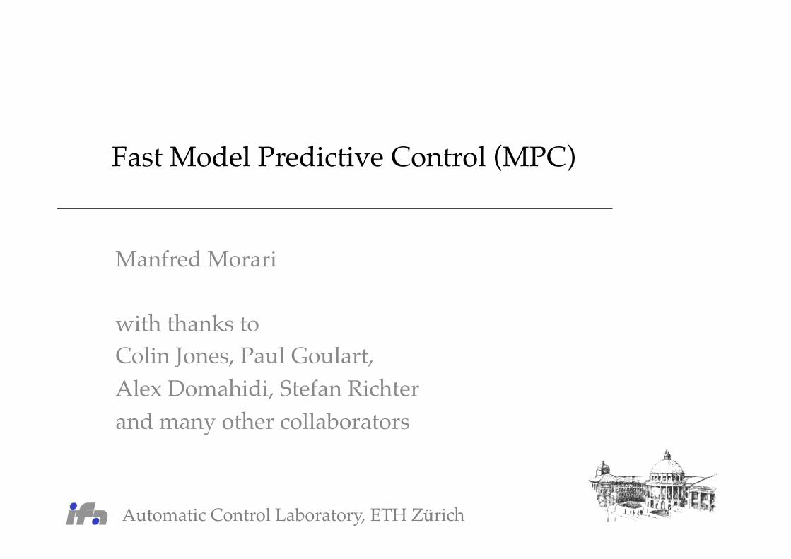
Published: 20.09.13
ETH President Ralph Eichler (r)congratulates his successor on hiselection. "I am very happy andproud at the confidence which theFederal Council and ETH Boardhave placed in me", Lino Guzzellacomments. He will be taking uphis duties on 1 January 2015.(large view)
Campus
The Swiss Federal Council has appointed Lino Guzzella, ETHRector and Professor of Thermotronics, as the future ETHPresident. He will be taking over from Ralph Eichler who isretiring at the end of 2014. By taking this decision, the SwissGovernment has endorsed the unanimous proposal made bythe ETH Board.
Norbert Staub
The timetable for the election of thenext President of ETH Zurichstipulated that the ETH Board wasto submit a proposal to the SwissFederal Council in winter 2013/14.In fact everything went aheadfaster than anticipated. By mid-April 2013, the closing date forsubmissions, a total of some 50applications and third partynominations were received inresponse to the ETH Board’sannouncement of the vacancy. TheETH Board went on to assess andshort list the candidates with theparticipation of two consultativevotes on behalf of ETH Zurich. ETHRector Lino Guzzella gaveimpressive confirmation to theselection board and Federal Council
as the appointing authority that he was the right person to lead ETHZurich into the future.
“Pride and respect”“I am very happy and proud at the confidence which the FederalCouncil and ETH Board have placed in me”, Lino Guzzella said abouthis election. “but I also have immense respect for the responsibility ofbeing asked to lead ETH, one of the finest universities of technology.To my mind, there is no more honourable position in the Swissscientific community, but also no more challenging task, than to serveas President of ETH Zurich.”
ETH President Ralph Eichler is delighted that a member of the existingschool management is to succeed him. “I congratulate Lino Guzzellasincerely on his election and am delighted that he proved to be thebest candidate in this challenging, international appointmentprocedure,” Ralph Eichler comments. “I have got to know andappreciate Lino Guzzella as a highly capable, dedicated andconstructive member of the school management and I am convincedthat he will advance the cause of ETH Zurich in years to come with thesupport of the professors and school management.” The ETHPresident continued: “For just over one more year, I will continue to
ShareShareMore
Lino Guzzella appointed President of ETHZurich

Automatic Control Laboratory, ETH Zürich!
Fast Model Predictive Control (MPC)"!
Manfred Morari!!with thanks to !Colin Jones, Paul Goulart, !Alex Domahidi, Stefan Richter!and many other collaborators!!
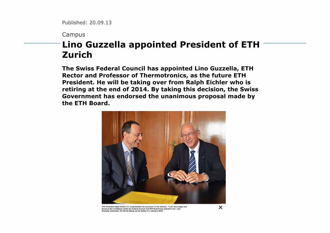
Dynamic Programming
Synthesis of Optimal Control Laws!Infinite-Horizon Optimal Control
J�(x) = minui⇤U
⇥�
i=0
l(xi, ui)
s.t. xi+1 = f(xi, ui)
xi � X
• Challenge is computation!!
J�(x) = minu
l(x, u) + J�(f(x, u))
s.t. (f(x, u), u) ⇥ X � U

Dynamic Programming
Synthesis of Optimal Control Laws!Infinite-Horizon Optimal Control
J�(x) = minui⇤U
⇥�
i=0
l(xi, ui)
s.t. xi+1 = f(xi, ui)
xi � X
• Challenge is computation!!• Closed-form solution for
linear systems, no constraints only: "LQR,…!
J�(x) = minu
l(x, u) + J�(f(x, u))
s.t. (f(x, u), u) ⇥ X � U

Dynamic Programming Model Predictive Control
Synthesis of Optimal Control Laws!Infinite-Horizon Optimal Control
J�(x) = minui⇤U
⇥�
i=0
l(xi, ui)
s.t. xi+1 = f(xi, ui)
xi � X
Explicit calculation of control law !offline!
Online optimization problem defines control action
J�(x) = minu
l(x, u) + J�(f(x, u))
s.t. (f(x, u), u) ⇥ X � U
u�(x) u�0(x)
J
⇤(x0) = minui
NX
i=0
l(xi, ui) + Vf (xN )
s.t. (xi, ui) 2 X ⇥ U, xN 2 Xf
xi+1 = f(xi, ui)
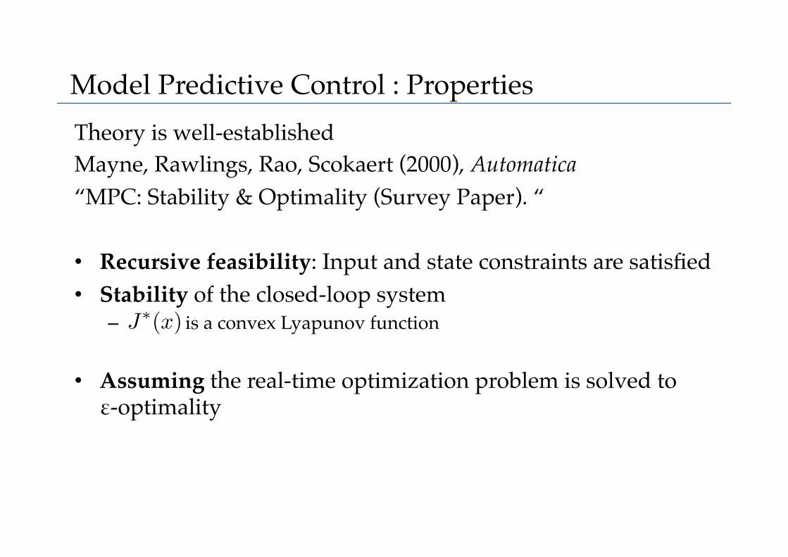
Model Predictive Control : Properties!Theory is well-established!Mayne, Rawlings, Rao, Scokaert (2000), Automatica !“MPC: Stability & Optimality (Survey Paper). “!!• Recursive feasibility: Input and state constraints are satisfied!• Stability of the closed-loop system!
– is a convex Lyapunov function!
• Assuming the real-time optimization problem is solved to #-optimality!
J�(x)

17
Traditional MPC!
• Successful in process industries!• Sampling times of minutes!• Powerful computing platforms!
• Small, high performance plants!• Sampling times of ms to ns!• Limited embedded platform!
Embedded MPC!
Embedded Model Predictive Control!
18
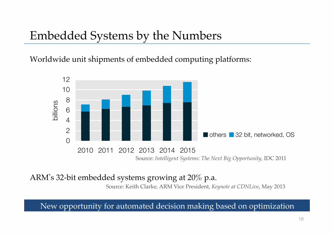
Embedded Systems by the Numbers!
Worldwide unit shipments of embedded computing platforms:!
!ARM’s 32-bit embedded systems growing at 20% p.a.!
02468
1012
2010 2011 2012 2013 2014 2015
billio
ns
others 32 bit, networked, OS
Source: Intelligent Systems: The Next Big Opportunity, IDC 2011!
Source: Keith Clarke, ARM Vice President, Keynote at CDNLive, May 2013 !
New opportunity for automated decision making based on optimization!
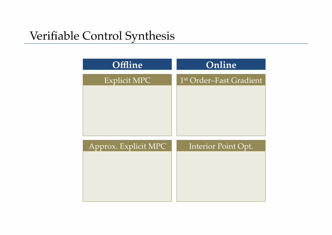
Verifiable Control Synthesis!
Offline Online Explicit MPC 1st Order–Fast Gradient
Approx. Explicit MPC Interior Point Opt.
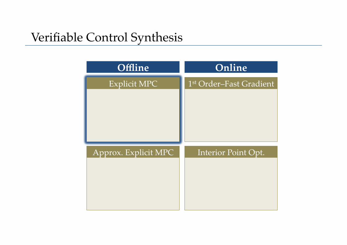
Verifiable Control Synthesis!
Offline Online Explicit MPC 1st Order–Fast Gradient
Approx. Explicit MPC Interior Point Opt.
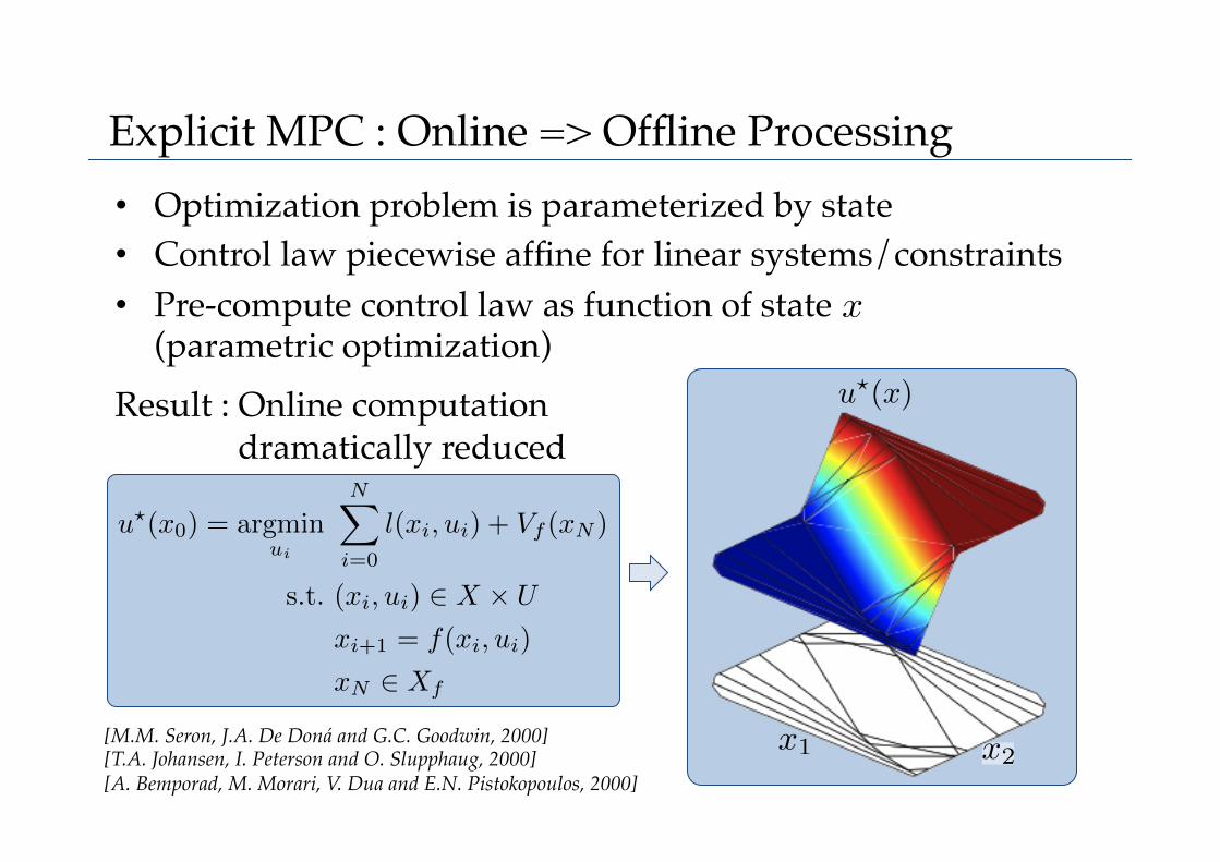
Explicit MPC : Online => Offline Processing!• Optimization problem is parameterized by state!• Control law piecewise affine for linear systems/constraints!• Pre-compute control law as function of state "
(parametric optimization)!Result : Online computation "
!dramatically reduced!u�(x)
x1 x2[M.M. Seron, J.A. De Doná and G.C. Goodwin, 2000] [T.A. Johansen, I. Peterson and O. Slupphaug, 2000] [A. Bemporad, M. Morari, V. Dua and E.N. Pistokopoulos, 2000]
x
u�(x0) = argminui
N�
i=0
l(xi, ui) + Vf (xN )
s.t. (xi, ui) ⇥ X � U
xi+1 = f(xi, ui)
xN ⇥ Xf
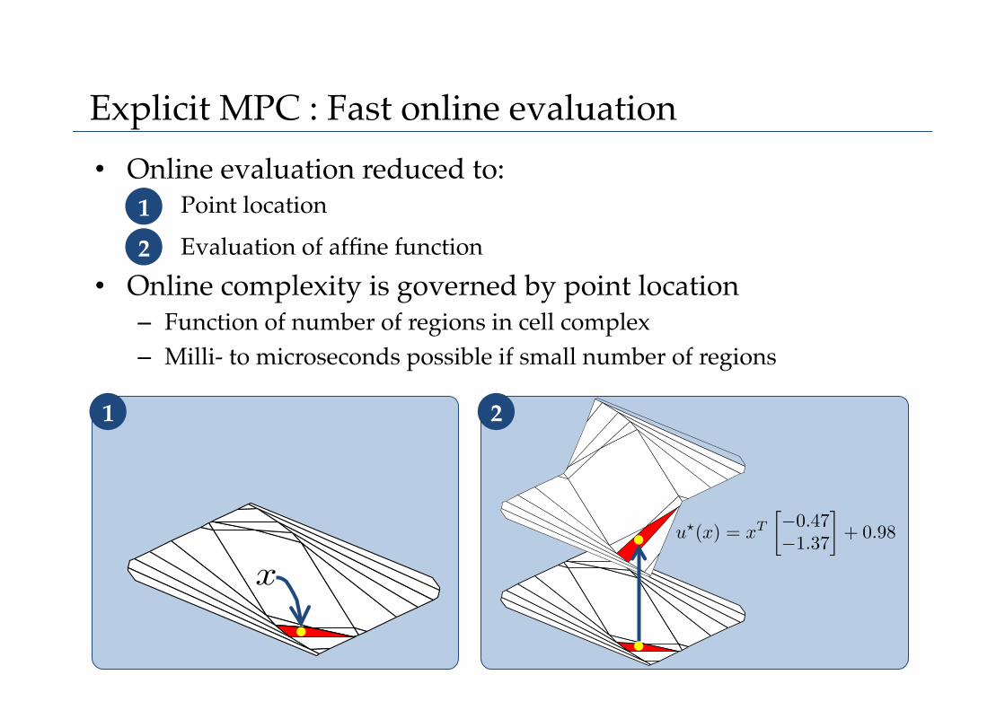
Explicit MPC : Fast online evaluation!• Online evaluation reduced to:!
1. Point location!2. Evaluation of affine function!
• Online complexity is governed by point location!– Function of number of regions in cell complex!– Milli- to microseconds possible if small number of regions!
x
u�(x) = xT
��0.47�1.37
⇥+ 0.98
1 2
1
2

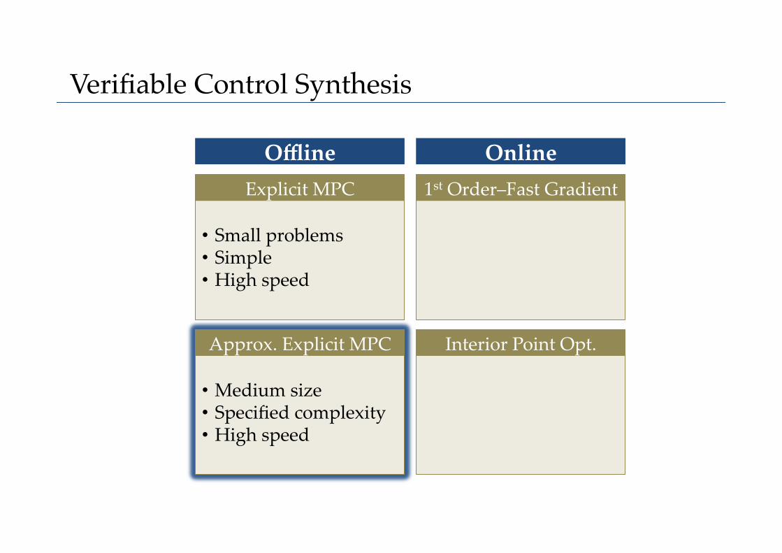
Verifiable Control Synthesis!
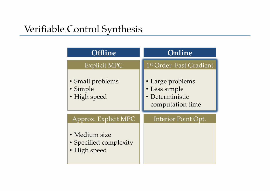
• Small problems • Simple • High speed
Offline Online Explicit MPC 1st Order–Fast Gradient
Approx. Explicit MPC Interior Point Opt.
Verifiable Control Synthesis!
• Small problems • Simple • High speed
• Medium size • Specified complexity • High speed
Offline Online Explicit MPC 1st Order–Fast Gradient
Approx. Explicit MPC Interior Point Opt.
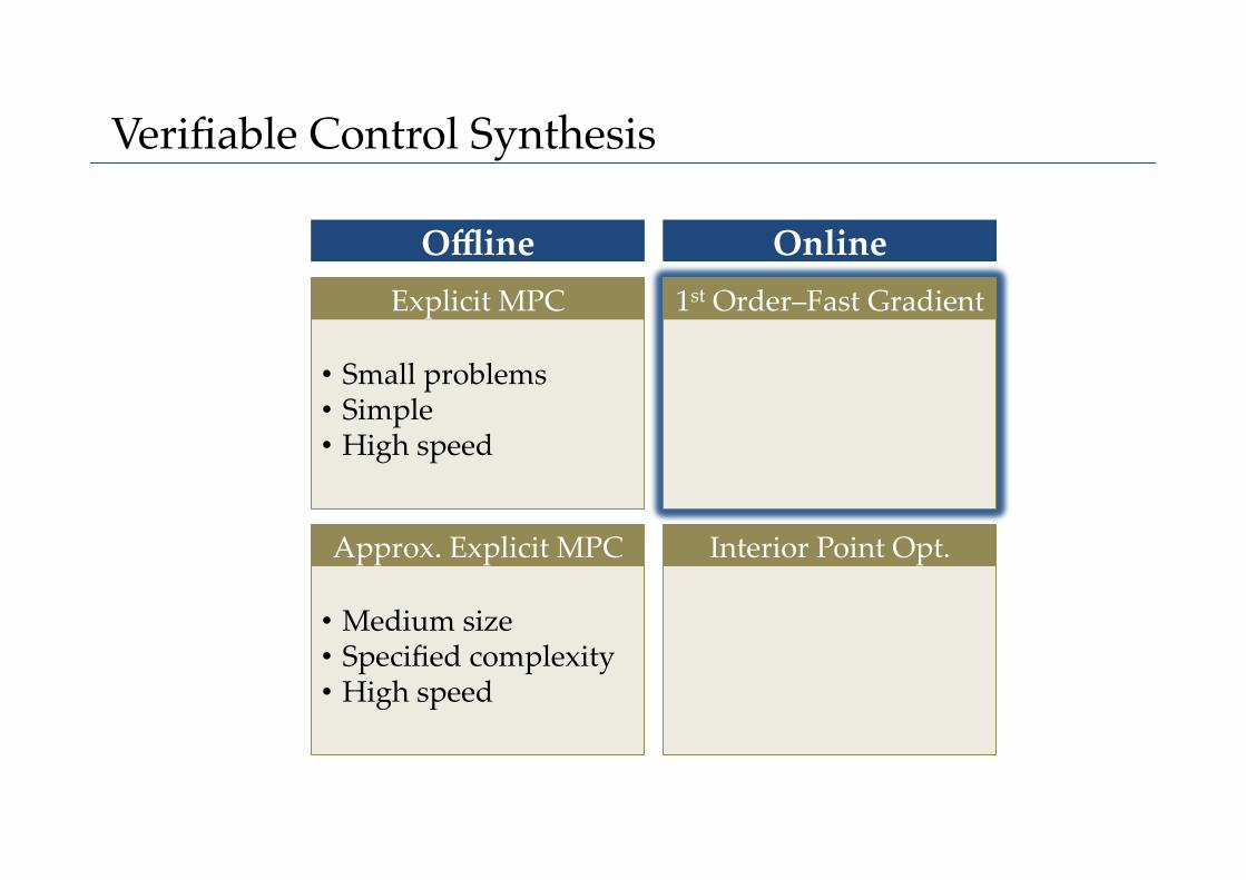
Verifiable Control Synthesis!
• Small problems • Simple • High speed
• Medium size • Specified complexity • High speed
Offline Online Explicit MPC 1st Order–Fast Gradient
Approx. Explicit MPC Interior Point Opt.

Fast Gradient Method : Time bound to ε-optimality!• ε-solution in imin steps!
• κ condition number!• δ measure of initial error!
• Asdf
• R : radius of feasible set • Easy to compute
Cold start • asdf
• Uw : Warm start solution • Worst distance measured in
terms of initial cost • Hard to compute
Warm start � = LR2/2 � = 2max
x⇥X0
JN (Uw;x)� J�N (x)
[Y. Nesterov, 1983] [S. Richter, C.N. Jones and M. Morari, CDC 2009]
imin ⇥
⇤
⇧⇧⇧⇧
ln �⇥
� ln�1�
⌥1⇤
⇥
⌅
⌃⌃⌃⌃
Verifiable Control Synthesis!
• Small problems • Simple • High speed
• Large problems • Less simple • Deterministic
computation time
• Medium size • Specified complexity • High speed
Offline Online Explicit MPC 1st Order–Fast Gradient
Approx. Explicit MPC Interior Point Opt.

Verifiable Control Synthesis!
• Small problems • Simple • High speed
• Large problems • Less simple • Deterministic
computation time
• Medium size • Specified complexity • High speed
Offline Online Explicit MPC 1st Order–Fast Gradient
Approx. Explicit MPC Interior Point Opt.
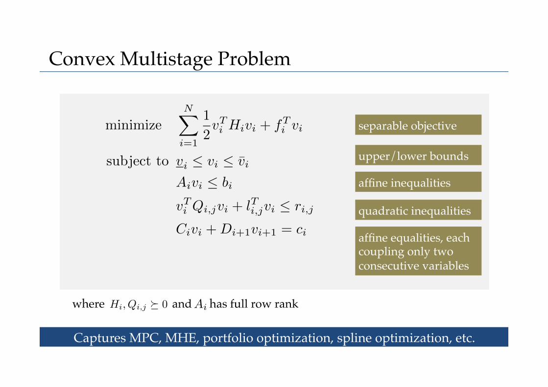
Convex Multistage Problem!
where and has full row rank!
upper/lower bounds!
affine inequalities!
quadratic inequalities!
affine equalities, each coupling only two consecutive variables!
separable objective!
Captures MPC, MHE, portfolio optimization, spline optimization, etc.!
minimizeN�
i=1
1
2vT
i Hivi + fTi vi
subject to vi � vi � vi
Aivi � bi
vTi Qi,jvi + lTi,jvi � ri,j
Civi + Di+1vi+1 = ci
Hi, Qi,j � 0 Ai
62
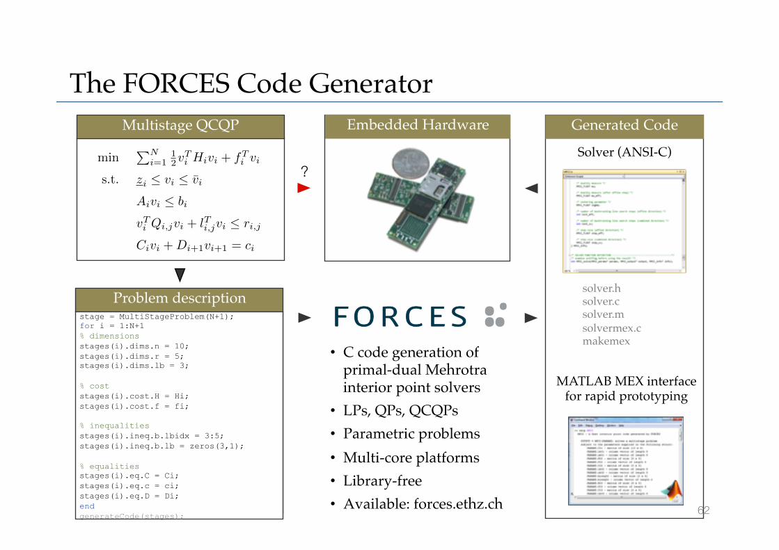
The FORCES Code Generator!Multistage QCQP!
?
Embedded Hardware!
• C code generation of primal-dual Mehrotra interior point solvers!
• LPs, QPs, QCQPs!• Parametric problems!• Multi-core platforms!• Library-free!• Available: forces.ethz.ch!
Problem description!stage = MultiStageProblem(N+1); for i = 1:N+1 % dimensions stages(i).dims.n = 10; stages(i).dims.r = 5; stages(i).dims.lb = 3; % cost stages(i).cost.H = Hi; stages(i).cost.f = fi; % inequalities stages(i).ineq.b.lbidx = 3:5; stages(i).ineq.b.lb = zeros(3,1); % equalities stages(i).eq.C = Ci; stages(i).eq.c = ci; stages(i).eq.D = Di; end generateCode(stages);
Solver (ANSI-C)!
MATLAB MEX interface"for rapid prototyping!
solver.h!solver.c!solver.m!solvermex.c!makemex!
Generated Code!
min�N
i=112vT
i Hivi + fTi vi
s.t. zi � vi � vi
Aivi � bi
vTi Qi,jvi + lTi,jvi � ri,j
Civi + Di+1vi+1 = ci

63
Speedups Compared to IBM’s CPLEX!
• Standard MPC problem for oscillating "chain of masses (on Intel i5 @3.1 GHz)!
• CPLEX N/A on embedded systems!
CPLEX!Solve time: 5470 $s Code size: 11700 KB!
FORCES!Solve time: 90 $s Code size: 52 KB!
80x!
10x!2x!

64
Some Early Users of FORCES!
MPC for Wind Turbines!Marc Guadayol, ALSTOM, 2012!
Adaptive MPC for Belt Drives!Kim Listmann, ABB Ladenburg, 2012!
Nonlinear MPC & MHE with ACADO!Milan Vukov, KU Leuven, 2012!
Quadrotor Control!Marc Müller, IDSC, ETH Zurich, 2012!
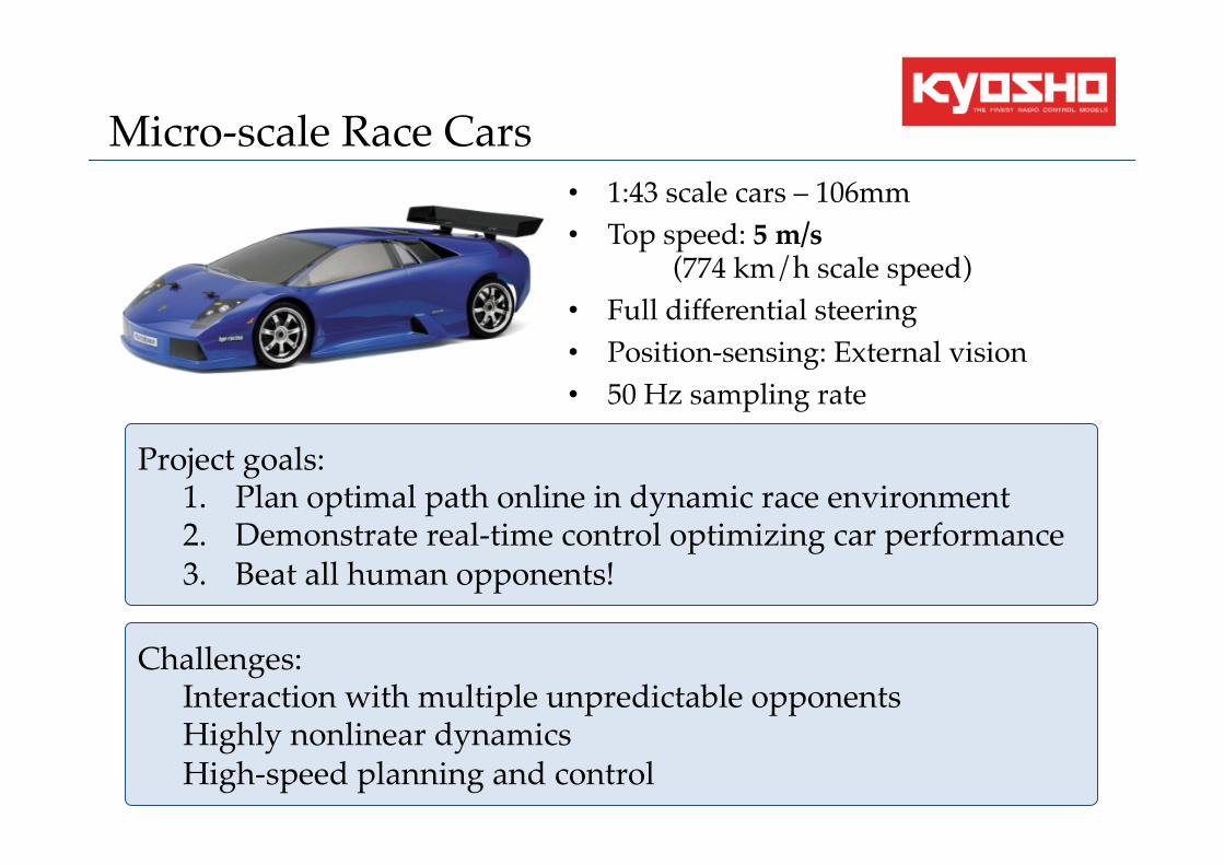
Challenges: Interaction with multiple unpredictable opponents Highly nonlinear dynamics High-speed planning and control
Project goals: 1. Plan optimal path online in dynamic race environment 2. Demonstrate real-time control optimizing car performance 3. Beat all human opponents!
Micro-scale Race Cars!• 1:43 scale cars – 106mm!• Top speed: 5 m/s "
!(774 km/h scale speed)!• Full differential steering!• Position-sensing: External vision!• 50 Hz sampling rate!

System Details!
Camera System
• Infrared spotlight • Reflectors on cars • 3.36 mm accuracy • 100 Hz update rate at
1024 x 1200 pixels
Embedded Board
• Custom built electronics • Bluetooth communication • IMUs & Gyro • H-bridges for DC Motors • ARM Cortex M4
Tracks
• Custom built high grip track
• Standard RCPtracks track
h!p://orcaracer.ethz.ch

Car Model and Model Analysis!
Analysis of zero accelerations (for fixed velocities) yield bifurcation:
Stationary velocities for vx = 1.5
Stationary trajectories are circles, where the radius is related to the forward velocity and the yaw rate
Car Model Model Analysis
Bicycle model with nonlinear lateral tire friction laws using a simplified Pacejka tire model:
x = vx cos � � vy sin �
y = vx sin � + vy cos �
� = �
vx =1
m(Frx(D) � Ffy sin � + mvy�)
vy =1
m(Fry(�r) + Ffy cos � � mvx�)
� =1
Jz(�Frylr + Ffy cos �lr)
� = const
vx = const
� = 0
vy = 0
steering angle δ [rad] steering angle δ [rad]
late
ral s
peed
vy [
m/s
]
yaw
rate
[rad
/s]

Path Planner and MPC!
• Trajectory tracking MPC formulation:!– re-linearizing the dynamics around trajectory!– linear constraints to stay on track / avoid obstacles!– 6 states, 2 inputs, horizon 16!
• Computation times on Intel Core i7 CPU @2.5 GHz:!
Reference trajectory generation! 4.13 ms!Problem data generation! 1.19 ms!Solving QP with CPLEX! 6.00 ms!Solving QP with FORCES! 0.83 ms!
minN�1�
i=0
(xi � xrefi )T Q(xi � xref
i ) + (ui � urefi )T R(ui � uref
i ) + (xN � xrefN )T P (xN � xref
N )
s.t. x0 = x
xi+1 = Aixi + Biui + gi
Gixi � hi
(xi, ui) � X � U
3.3 ms on ARM Cortex A9 @1.7 GHz
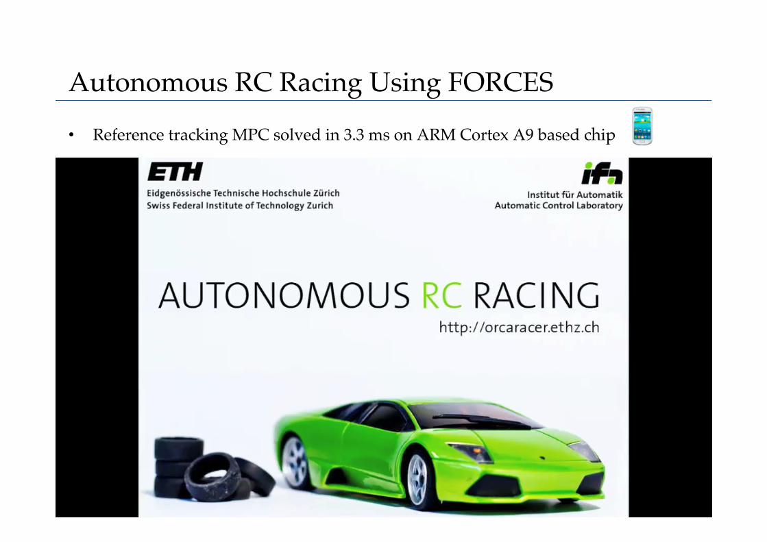
Autonomous RC Racing Using FORCES!
• Reference tracking MPC solved in 3.3 ms on ARM Cortex A9 based chip!
[A. Liniger, 2013]!
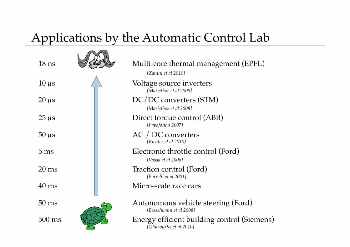
Applications by the Automatic Control Lab!
18 ns !Multi-core thermal management (EPFL)"! ![Zanini et al 2010] !
10 µs !Voltage source inverters !"! ![Mariethoz et al 2008]!
20 µs !DC/DC converters (STM) ! !!! ! ![Mariethoz et al 2008]!
25 µs !Direct torque control (ABB) !"! ![Papafotiou 2007]!
50 µs !AC / DC converters !"! ![Richter et al 2010]!
5 ms !Electronic throttle control (Ford) !!! ! ![Vasak et al 2006]!
20 ms !Traction control (Ford) !"! ![Borrelli et al 2001]!
40 ms !Micro-scale race cars "! !!
50 ms !Autonomous vehicle steering (Ford)"! ![Besselmann et al 2008]!
500 ms !Energy efficient building control (Siemens) !"! ![Oldewurtel et al 2010]!

77
Hardware architectures for fast-gradient and ADMM methods parameterized by:!• Degree of parallelism!• Fixed-point computing precision!
Fixed-point arithmetic analysis:!• ensures reliable operation!• Solution accuracy specs # bits!
!
~250 variable optimization problem:!
State-of-the-art:!✦ ~5 ms!
✦ Desktop @ 3GHz!✦ ~70 Watts!
FPGAs:!✦ ~0.5 $s !
✦ Embedded @ 400MHz!✦ ~5 Watts!
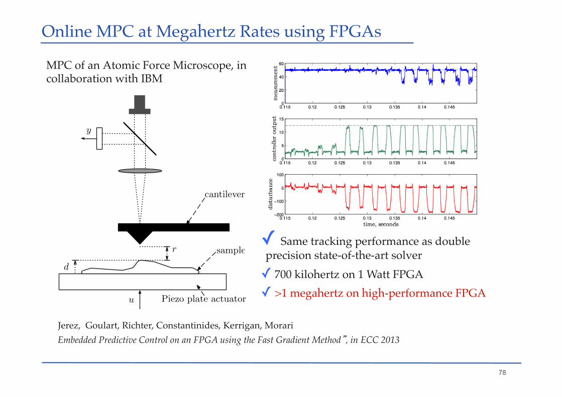
Online MPC at Megahertz Rates using FPGAs!
10 20 30 40 50 60 70 80 90 10010−8
10−7
10−6
10−5
10−4
10−3
10−2
10−1
100Convergence rate of ADMM
||z!(x)"
zi||2
Number of ADMM iterations i
doubleb=18b=24b=32
78
MPC of an Atomic Force Microscope, in collaboration with IBM!
Jerez, Goulart, Richter, Constantinides, Kerrigan, Morari Embedded Predictive Control on an FPGA using the Fast Gradient Method”, in ECC 2013
✓ Same tracking performance as double precision state-of-the-art solver!✓ 700 kilohertz on 1 Watt FPGA!✓ >1 megahertz on high-performance FPGA !
Online MPC at Megahertz Rates using FPGAs!
y
d
r
cantilever
sample
Piezo plate actuatoru
Conclusions!• Computation technology is not limiting the application of
MPC at any speed for any size problem!• When and where to employ MPC in industry is still a matter
of judgment (modeling, maintenance, robustness)!

!
Thank you, Keith!


![SWIFT: Predictive Fast Reroute - CAIDASWIFT: Predictive Fast Reroute SIGCOMM ’17, August 21-25, 2017, Los Angeles, CA, USA transit [60]), it does not know any backup path forS6 andS8:](https://img.pdfslide.us/doc/110x75/5e97b2e7bd3bcc39d12838b3/swift-predictive-fast-reroute-swift-predictive-fast-reroute-sigcomm-a17-august.jpg)


![Fast Calibration of a Robust Model Predictive Controller ... · arXiv:1804.06161v1 [cs.SY] 17 Apr 2018 Fast Calibration of a Robust Model Predictive Controller for Diesel Engine Airpath](https://img.pdfslide.us/doc/110x75/5cef025f88c993f1758dc0f6/fast-calibration-of-a-robust-model-predictive-controller-arxiv180406161v1.jpg)