Fast Coordinate Descent Methods with Variable Selection

for Non-Negative Matrix Factorization

Cho-Jui Hsieh and Inderjit S. Dhillon

Department of Computer Science

The University of Texas at Austin

{cjhsieh,inderjit}@cs.utexas.edu

February 22, 2011

Abstract

Nonnegative Matrix Factorization (NMF) is an effective dimension reductionmethod for non-negative dyadic data, and has proven to be useful in many ar-eas, such as text mining, bioinformatics and image processing. The mathemat-ical formulation of NMF is a constrained non-convex optimization problem, andmany algorithms have been developed for solving it. Recently, a coordinate descentmethod, called FastHals [3], has been proposed to solve least squares NMF and isregarded as one of the state-of-the-art techniques for the problem. In this paper,we first show that FastHals has an inefficiency in that it uses a cyclic coordinatedescent scheme and thus, performs unneeded descent steps on unimportant vari-ables. We then present a variable selection scheme that uses the gradient of theobjective function to arrive at a new coordinate descent method. Our new methodis considerably faster in practice and we show that it has theoretical convergenceguarantees. Moreover when the solution is sparse, as is often the case in real appli-cations, our new method benefits by selecting important variables to update moreoften, thus resulting in higher speed. As an example, on a text dataset RCV1,our method is 7 times faster than FastHals, and more than 15 times faster whenthe sparsity is increased by adding an L1 penalty. We also develop new coordinatedescent methods when error in NMF is measured by KL-divergence by applyingthe Newton method to solve the one-variable sub-problems. Experiments indicatethat our algorithm for minimizing the KL-divergence is faster than the Lee & Seungmultiplicative rule by a factor of 10 on the CBCL image dataset.

1 Introduction

Non-negative matrix factorization (NMF) ([18, 13]) is a popular matrix decompositionmethod for finding non-negative representations of data. NMF has proved useful indimension reduction of image, text, and signal data. Given a matrix V ∈ R

m×n, V ≥ 0,and a specified positive integer k, NMF seeks to approximate V by the product of twonon-negative matrix W ∈ R

m×k and H ∈ Rk×n. Suppose each column of V is an

input data vector, the main idea behind NMF is to approximate these input vectors by

1

nonnegative linear combinations of nonnegative “basis” vectors (columns of W ) withthe coefficients stored in columns of H.

The distance between V and WH can be measured by various distortion functions— the most commonly used is the Frobenius norm, which leads to the following mini-mization problem:

minW,H≥0

f(W, H)≡1

2‖V − WH‖2

F =1

2

∑

i,j

(Vij − (WH)ij)2 (1)

To achieve better sparsity, researchers ([7, 19]) have proposed adding regularizationterms, on W and H, to (1). For example, an L1-norm penalty on W and H can achievea more sparse solution:

minW,H≥0

1

2‖V − WH‖2

F + ρ1

∑

i,r

Wir + ρ2

∑

r,j

Hrj . (2)

One can also replace∑

i,r Wir and∑

r,j Hrj by Frobenius norm of W and H. Notethat usually m ≫ k and n ≫ k. Since f is non-convex, we can only hope to find astationary point of f . Many algorithms ([14, 5, 1, 20]) have been proposed for thispurpose. Among them, the Lee & Seung’s multiplicative-update algorithm [14] hasbeen the most common method. Recent methods follow the alternating nonnegativeleast squares (ANLS) framework suggested by [18]. This framework has been proved toconverge to stationary points by [6] as long as one can solve each nonnegative least squaresub-problem exactly. [16] proposes a projected gradient method, [10] uses an active setmethod, [9] applies a projected Newton method, and [11] suggests a modified active setmethod called BlockPivot for solving the non-negative least square sub-problem. Veryrecently, [17] developed a parallel NMF solver for large-scale web data. This showsa practical need for further scaling up NMF solvers, especially when the matrix V issparse, as is the case for text data or web recommendation data.

Coordinate descent methods, which update one variable at a time, are efficient atfinding a reasonable solution efficiently, a property that has made these methods suc-cessful in large scale classification/regression problems. Recently, a coordinate descentmethod, called FastHals [3], has been proposed to solve the least squares NMF prob-lem (1). Compared to methods using the ANLS framework which spend significanttime in finding an exact solution for each sub-problem, a coordinate descent methodcan efficiently give a reasonably good solution for each sub-problem and switch to thenext round. Despite being a state-of-the-art method, FastHals has an inefficiency inthat it uses a cyclic coordinate descent scheme and thus, performs unneeded descentsteps on unimportant variables. In this paper, we present a variable selection schemethat uses the gradient of the objective function to arrive at a new coordinate descentmethod. Our method is considerably faster in practice and we show that it has theoret-ical convergence guarantees, which was not addressed in [3]. To scale our algorithm up,we also conduct experiments on large sparse datasets. Our method generally performs 4times faster than FastHals. Moreover when the solution is sparse, as is often the case inreal applications, our new method benefits by selecting important variables to update

2

more often, thus resulting in higher speed. As an example, on a text dataset RCV1,our method is 7 times faster than FastHals, and more than 15 times faster when thesparsity is increased by adding an L1 penalty.

Another popular distortion measure to minimize is the KL-divergence between Vand WH:

minW,H≥0

L(W, H) =∑

i,j

Vij log(Vij

(WH)ij) − Vij + (WH)ij (3)

The above problem has been shown to be connected to Probabilistic Latent SemanticAnalysis (PLSA) [4]. As we will point out in Section 3, problem (3) is more complicatedthan (1) and algorithms in the ANLS framework cannot be easily extended to solve (3).For this problem, [3] proposes to solve by a sequence of local loss functions — however, adrawback of the method in [3] is that it will not converge to the stationary point of (3).In this paper we propose a cyclic coordinate descent method for solving (3). Our newalgorithm applies Newton method to get better solution for each variable, which is bettercompared to working on the auxiliary function as used in multiplicative algorithm by[14]. As the result, our cyclic coordinate descent method converges much faster thanmultiplicative algorithm. We further provide theoretical convergence guarantees forcyclic coordinate descent methods under certain conditions.

The paper is organized as follows. In Section 2, we describe our coordinate descentmethod for least squares NMF (1). The modification for the coordinate descent methodfor solving KL divergence problem (3) is proposed in Section 3. Section 4 discuss therelationship between our methods and other optimization techniques for NMF, andSection 5 points out some important implementation issue. The experiment results aregiven in Section 6. The results show that our method in square error and KL divergenceare more efficient than other state-of-art methods.

2 Coordinate Descent Method for Least Squares NMF

2.1 Basic update rule for one element

The coordinate descent method updates one variable at a time until converge. We firstshow that a closed form update can be performed in O(1) time for least squares NMFif certain quantities have been pre-computed. Note that in this section we focus on theupdate rule for variables in W — the update rule for variables in H can be derivedsimilarly.

Coordinate descent methods aim to conduct the following one variable updates:

(W, H) ← (W + seir, H)

where eir is a m×k matrix with all elements zero except the (i, r) element which equalsone. Coordinate descent solves the following one-variable subproblem of (1) to get s:

mins:Wir+s≥0

gWir (s) ≡ f(W + seir, H). (4)

3

We can rewrite gWir (s) as

gWir (s) =

1

2

∑

j

(Vij − (WH)ij − sHrj)2 (5)

= gWir (0) + (gW

ir )′(0)s +1

2(gW

ir )′′(0)s2. (6)

For convenience we define

GW ≡ ∇W f(W, H) = WHHT − V HT . (7)

and GH ≡ ∇Hf(W, H) = W T WH − W T V. (8)

Then we have

(gWir )′(0) = (GW )ir = (WHHT − V HT )ir

and (gWir )′′(0) = (HHT )rr.

Since (6) is a one-variable quadratic function with the constraint Wir + s ≥ 0, we cansolve it in closed form:

s∗ = max

(

0, Wir −(WHHT − V HT )ir

(HHT )rr

)

− Wir. (9)

Coordinate descent algorithms then update Wir to

Wir ← Wir + s∗. (10)

The above one variable update rule can be easily extended to NMF problems withregularization as long as the gradient and second order derivative of sub-problems canbe easily computed. For instance, with the L1 penalty on both W and H as in (2), theone variable sub-problem is

gWir (s) =

(

(WHHT − V HT )ir + ρ1

)

s +1

2(HHT )rrs

2 + gWir (0),

and thus the one variable update becomes

Wir ← max

(

0, Wir −(WHHT − V HT )ir + ρ1

(HHT )rr

)

.

Compared to (9), the new Wir is shifted left to zero by the factor ρ1

(HHT )rr, so the

resulting Wir has more zeros.A state-of-the-art cyclic coordinate descent method called FastHals is proposed in [3],

which uses the above one variable update rules.

4

0 2 4 6 8 10

x 107

6.2

6.4

6.6

6.8

7

7.2

7.4

7.6

7.8x 10

4

Number of Coordinate Updates

Obj

ectiv

e V

alue

CDFastHals

(a) Coordinate updates versusobjective value

0 0.5 1 1.5 2

x 106

0

1

2

3

4

5

nu

mb

er

of

up

da

tes

0 0.5 1 1.5 2

x 106

0

1

2

3

4

5x 10

−3

variables in H

valu

es

in t

he

so

lutio

n

(b) The behavior of FastHals (c) The behavior of GCD

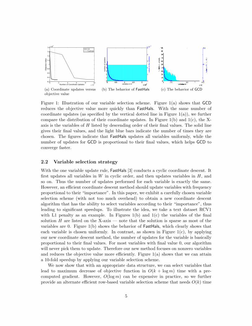
Figure 1: Illustration of our variable selection scheme. Figure 1(a) shows that GCD

reduces the objective value more quickly than FastHals. With the same number ofcoordinate updates (as specified by the vertical dotted line in Figure 1(a)), we furthercompare the distribution of their coordinate updates. In Figure 1(b) and 1(c), the X-axis is the variables of H listed by descending order of their final values. The solid linegives their final values, and the light blue bars indicate the number of times they arechosen. The figures indicate that FastHals updates all variables uniformly, while thenumber of updates for GCD is proportional to their final values, which helps GCD toconverge faster.

2.2 Variable selection strategy

With the one variable update rule, FastHals [3] conducts a cyclic coordinate descent. Itfirst updates all variables in W in cyclic order, and then updates variables in H, andso on. Thus the number of updates performed for each variable is exactly the same.However, an efficient coordinate descent method should update variables with frequencyproportional to their “importance”. In this paper, we exhibit a carefully chosen variableselection scheme (with not too much overhead) to obtain a new coordinate descentalgorithm that has the ability to select variables according to their “importance”, thusleading to significant speedups. To illustrate the idea, we take a text dataset RCV1with L1 penalty as an example. In Figures 1(b) and 1(c) the variables of the finalsolution H are listed on the X-axis — note that the solution is sparse as most of thevariables are 0. Figure 1(b) shows the behavior of FastHals, which clearly shows thateach variable is chosen uniformly. In contrast, as shown in Figure 1(c), by applyingour new coordinate descent method, the number of updates for the variable is basicallyproportional to their final values. For most variables with final value 0, our algorithmwill never pick them to update. Therefore our new method focuses on nonzero variablesand reduces the objective value more efficiently. Figure 1(a) shows that we can attaina 10-fold speedup by applying our variable selection scheme.

We now show that with an appropriate data structure, we can select variables thatlead to maximum decrease of objective function in O(k + log m) time with a pre-computed gradient. However, O(log m) can be expensive in practice, so we furtherprovide an alternate efficient row-based variable selection scheme that needs O(k) time

5

per update.Before presenting our variable selection method, we first introduce our framework.

Similar to FastHals, our algorithm switches between W and H in the outer iterations:

(W 0, H0) → (W 1, H0) → (W 1, H1) → · · · (11)

Between each outer iteration, we conduct the following inner updates:

(W i, H i) → (W i,1, H i) → (W i,2, H i) · · · . (12)

Later we will discuss the reason why we have to focus on W or H for a sequence ofupdates.

Suppose we want to choose variables to update in W . If Wir is selected, as discussedin Section 2.1, the optimal update will be (9), and the function value will be decreasedby

DWir ≡ gW

ir (s∗) − gWir (0) = GW

ir s∗ +1

2(HHT )rr(s

∗)2. (13)

DWir measures how much we can reduce the objective value by choosing the coordinate

Wir. Therefore, if DW can be maintained, we can choose variables according to it. Ifwe have GW , we can compute s∗ by (9) and compute DW by (13), and so an elementof DW can be computed in O(1) time. At the beginning of a sequence of W ’s updates,we can precompute GW . The details will be provided in Section 2.3. Now assume wealready have GW , and Wir is updated to Wir + s∗. Then GW will remain the sameexcept for the ith row, which will be replaced by

GWij ← GW

ij + s∗(HHT )rj ∀j = 1, . . . , k. (14)

Using (14), we can maintain GW in O(k) time after each variable update of W . ThusDW can also be maintained in O(k) time.

However, maintaining GH at each inner update of W is more expensive. From (8),when each element of W is changed, the whole matrix GH will be changed, thus everyelement of DH may also change. So the time cost for maintaining DH is at least O(kn),which is too much compared to O(k) for maintaining DW . This is the reason that wefollow the alternative minimization scheme and restrict ourselves to either W or H fora sequence of inner updates.

After the i-th row of GW is updated, we can immediately maintain the i-th row ofDW by (13). To select the next variable-to-update, we want to select the index (i∗, r∗)that satisfies (i∗, r∗) = arg maxi,r DW

ir . However, a brute force search through the wholematrix DW will require O(mk) time. To overcome this, we can store the largest valuevi and index qi for each row of DW , i.e.,

qi = arg maxj

DWij , vi = DW

i,qi. (15)

As in (14), when Wir is updated, only the ith row of GW and DW will change. Thereforethe vector q will remain the same except for one component qi. Since the ith row of

6

DW contains k elements and each element can be computed in constant time, we canrecalculate qi in O(k) time. Each time we only change one of the values in {qi | i =1, . . . , m}, we can store these values using a heap data structure, so that each retrievaland re-calculation of the largest value can be done in O(log m) time. This way the totalcost for one update will be O(k + log m).

A stopping condition is needed for a sequence of updates. At the beginning ofupdates to W , we can store

pinit = maxi,j

DWij . (16)

Our algorithm then iteratively chooses variables to update until the following stoppingcondition is met:

maxi,j

DWij < ǫpinit, (17)

where ǫ is a small positive constant. Note that (17) will be satisfied in a finite numberof iterations as f(W, H) is strictly convex in W , and so the minimum for f(W, H) withfixed H is achievable. A small ǫ value indicates each sub-problem is solved to highaccuracy, while a larger ǫ value means our algorithm switches more often between Wand H. We choose ǫ = 0.001 in our experiments.

In practice, this method can work when k is large. However, when k ≪ m, thelog m term in the update cost will dominate. Moreover, each heap operation costs moretime than a simple floating point operation. Thus we further design a more efficientrow-based variable selection strategy.

First, we have an observation that when one Wir is updated, only the ith row ofDW will be changed. Therefore if we update variables in the ith row and there is avariable in the jth row with larger potential decrease DW

jr , we will not change DWjr .

Choosing the largest DW value in one row costs O(k), which is cheaper than O(log m)when k small. Therefore we can iteratively update variables in the ith row (that leadto maximum decrease in objective function) until the inner stopping condition is met:

maxj

DWij < ǫpinit. (18)

Our algorithm then update variables in the (i + 1)-st row, and so on. Since changesin other rows will not affect the DW values in the ith row, after our algorithm sweepsthrough row 1 to row m, (18) will be met for each row, thus the stopping condition (17)will also be met for the whole W .

2.3 Time complexity analysis

Our coordinate descent method with variable selection strategy can be summarized inAlgorithm 1. We call our new coordinate descent algorithm by GCD– Greedy CoordinateDescent since we take the greedy step of maximum decrease in objective function. Theone-variable update and variable selection strategy are in the inner loop (step 7) of thealgorithm. Before the inner loop, we have to initialize the gradient GW and objectivefunction decrease matrix DW . GW in (8) has two terms WHHT and V HT (in Algorithm

7

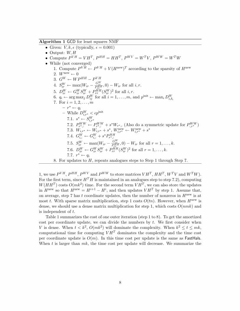
Algorithm 1 GCD for least squares NMF

• Given: V, k, ǫ (typically, ǫ = 0.001)• Output: W, H• Compute P V H = V HT , PHH = HHT , PWV = W T V , PWW = W T W• While (not converged)

1. Compute P V H ← P V H + V (Hnew)T according to the sparsity of Hnew

2. W new ← 03. GW ← WPHH − P V H

4. SWir ← max(Wir −

GWir

P HHrr

, 0) − Wir for all i, r.

5. DWir ← GW

ir SWir + PHH

rr (SWir )2 for all i, r.

6. qi ← arg maxj DWij for all i = 1, . . . , m, and pinit ← maxi D

Wi,δi

7. For i = 1, 2, . . . , m– r∗ ← qi

– While DWi,r∗ < ǫpinit

7.1. s∗ ← SWi,r∗

7.2. PWWr∗,: ← PWW

r∗,: + s∗Wr∗,: (Also do a symmetric update for PWW:,r∗ )

7.3. Wi,r∗ ← Wi,r∗ + s∗, W newi,r∗ ← W new

i,r∗ + s∗

7.4. GWi,: ← GW

i,: + s∗PHHr∗,:

7.5. SWir ← max(Wir −

GWir

P HHrr

, 0) − Wir for all r = 1, . . . , k.

7.6. DWir ← GW

ir SWir + PHH

rr (SWir )2 for all r = 1, . . . , k.

7.7. r∗ ← qi

8. For updates to H, repeats analogues steps to Step 1 through Step 7.

1, we use P V H , PHH , PWV and PWW to store matrices V HT , HHT , W T V and W T W ).For the first term, since HT H is maintained in an analogues step to step 7.2), computingW (HHT ) costs O(mk2) time. For the second term V HT , we can also store the updatesin Hnew so that Hnew = H i+1 − H i, and then updates V HT by step 1. Assume that,on average, step 7 has t coordinate updates, then the number of nonzeros in Hnew is atmost t. With sparse matrix multiplication, step 1 costs O(tn). However, when Hnew isdense, we should use a dense matrix multiplication for step 1, which costs O(nmk) andis independent of t.

Table 1 summarizes the cost of one outer iteration (step 1 to 8). To get the amortizedcost per coordinate update, we can divide the numbers by t. We first consider whenV is dense. When t < k2, O(mk2) will dominate the complexity. When k2 ≤ t ≤ mk,computational time for computing V HT dominates the complexity and the time costper coordinate update is O(m). In this time cost per update is the same as FastHals.When t is larger than mk, the time cost per update will decrease. We summarize the

8

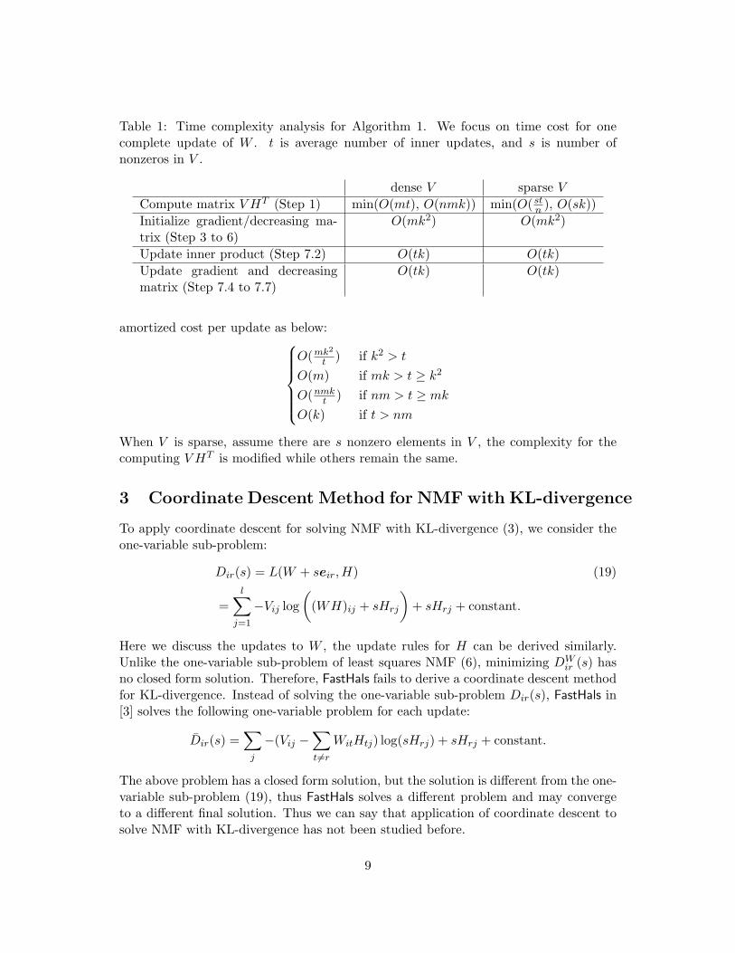
Table 1: Time complexity analysis for Algorithm 1. We focus on time cost for onecomplete update of W . t is average number of inner updates, and s is number ofnonzeros in V .

dense V sparse V

Compute matrix V HT (Step 1) min(O(mt), O(nmk)) min(O( stn ), O(sk))

Initialize gradient/decreasing ma-trix (Step 3 to 6)

O(mk2) O(mk2)

Update inner product (Step 7.2) O(tk) O(tk)

Update gradient and decreasingmatrix (Step 7.4 to 7.7)

O(tk) O(tk)

amortized cost per update as below:

O(mk2

t ) if k2 > t

O(m) if mk > t ≥ k2

O(nmkt ) if nm > t ≥ mk

O(k) if t > nm

When V is sparse, assume there are s nonzero elements in V , the complexity for thecomputing V HT is modified while others remain the same.

3 Coordinate Descent Method for NMF with KL-divergence

To apply coordinate descent for solving NMF with KL-divergence (3), we consider theone-variable sub-problem:

Dir(s) = L(W + seir, H) (19)

=

l∑

j=1

−Vij log

(

(WH)ij + sHrj

)

+ sHrj + constant.

Here we discuss the updates to W , the update rules for H can be derived similarly.Unlike the one-variable sub-problem of least squares NMF (6), minimizing DW

ir (s) hasno closed form solution. Therefore, FastHals fails to derive a coordinate descent methodfor KL-divergence. Instead of solving the one-variable sub-problem Dir(s), FastHals in[3] solves the following one-variable problem for each update:

Dir(s) =∑

j

−(Vij −∑

t6=r

WitHtj) log(sHrj) + sHrj + constant.

The above problem has a closed form solution, but the solution is different from the one-variable sub-problem (19), thus FastHals solves a different problem and may convergeto a different final solution. Thus we can say that application of coordinate descent tosolve NMF with KL-divergence has not been studied before.

9

In this paper, we propose the use of Newton’s method to solve the sub-problems.Since DW

ir is twice differentiable, we can iteratively update s by Newton direction:

s ← max

(

− Wir, s −D′

i(s)

D′′i (s)

)

, (20)

where the first term comes from the non-negativity constraint. The first derivativeD′

i(s) and the second derivative D′′i (s) can be written as

D′ir(s) =

n∑

j=1

Hrj

(

1 −Vij

(WH)ij + sHrj

)

. (21)

D′′ir(s) =

n∑

j=1

VijH2rj

((WH)ij + sHrj)2. (22)

For KL-divergence, we need to take care of the behavior when Vij = 0 or (WH)ij = 0.For Vij = 0, by analysing the asymptotic behavior, Vij log((WH)ij) = 0 for all positivevalues of (WH)ij , thus we can ignore those entries. Also, we do not consider the casethat one row of V is entirely zero, which can be removed by preprocessing. When(WH)ij + sHrj = 0 for some j, the Newton direction D′

ir(0)/D′′ir(0) should be zero. In

this situation we begin our search from a small arbitrary nonzero point s and restartthe search. When Hrj = 0 for all j = 1, . . . , n, the second derivative (22) is zero. Inthis case Dir(s) is constant, thus we do not need to change Wir.

To execute Newton updates, each evaluation of D′ir(s) and D′′

ir(s) takes O(n) timefor the summation. For general functions, we often need a line search procedure tocheck sufficient decrease from each Newton iteration. However, as we now deal withthe special function (19), we prove the following theorem to show that Newton methodwithout line search converges to the optimum of each sub-problem:

Theorem 1 If a function f(x) with domain x ≥ 0 can be written in the following form

f(x) = −ci

l∑

i=1

log(ai + bix) +∑

j

bix,

where ai > 0, bi, ci ≥ 0 ∀i, then the Newton method without line search converges to theglobal minimum of f(x).

The proof based on the strict convexity of log function is in Appendix 8.2. By the aboveTheorem, we can iteratively apply (20) until convergence. In practice, we design thefollowing stopping condition for Newton method:

|st+1 − st| < ǫ|Wir + st| for some ǫ > 0,

where st is the current solution and st+1 is obtained by (20).As discussed earlier, variable selection is an important issue for coordinate descent

methods. After each inner update Wir ← Wir + s∗, the gradient for Dit(s) will change

10

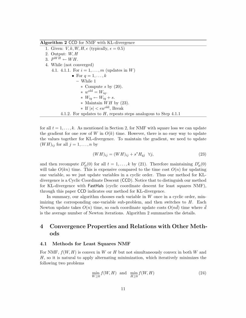
Algorithm 2 CCD for NMF with KL-divergence

1. Given: V, k, W, H, ǫ (typically, ǫ = 0.5)2. Output: W, H3. PWH ← WH.4. While (not converged)

4.1. 4.1.1. For i = 1, . . . , m (updates in W )• For q = 1, . . . , k

– While 1∗ Compute s by (20).∗ wold = Wiq.∗ Wiq ← Wiq + s.∗ Maintain WH by (23).∗ If |s| < ǫwold, Break

4.1.2. For updates to H, repeats steps analogous to Step 4.1.1

for all t = 1, . . . , k. As mentioned in Section 2, for NMF with square loss we can updatethe gradient for one row of W in O(k) time. However, there is no easy way to updatethe values together for KL-divergence. To maintain the gradient, we need to update(WH)ij for all j = 1, . . . , n by

(WH)ij = (WH)ij + s∗Hqj ∀j, (23)

and then recompute D′it(0) for all t = 1, . . . , k by (21). Therefore maintaining D′

it(0)will take O(kn) time. This is expensive compared to the time cost O(n) for updatingone variable, so we just update variables in a cyclic order. Thus our method for KL-divergence is a Cyclic Coordinate Descent (CCD). Notice that to distinguish our methodfor KL-divergence with FastHals (cyclic coordinate descent for least squares NMF),through this paper CCD indicates our method for KL-divergence.

In summary, our algorithm chooses each variable in W once in a cyclic order, min-imizing the corresponding one-variable sub-problem, and then switches to H. EachNewton update takes O(n) time, so each coordinate update costs O(nd) time where dis the average number of Newton iterations. Algorithm 2 summarizes the details.

4 Convergence Properties and Relations with Other Meth-

ods

4.1 Methods for Least Squares NMF

For NMF, f(W, H) is convex in W or H but not simultaneously convex in both W andH, so it is natural to apply alternating minimization, which iteratively minimizes thefollowing two problems

minW≥0

f(W, H) and minH≥0

f(W, H) (24)

11

until convergence. As mentioned in [9], we can categorize NMF solvers into two groups:exact methods and inexact methods. Exact methods are guaranteed to achieve optimumfor each sub-problem (24), while inexact methods only guarantee decrease in functionvalue. Each sub-problem for least squares NMF can be decomposed into a sequence ofnon-negative least square (NNLS) problems. For example, minimization with respect toH can be decomposed into minhi≥0 ‖V −Whi‖

2, where hi is the ith column of H. Sincethe convergence property for exact methods has been proved in [6], any NNLS solvercan be applied to solve NMF. This framework becomes the main strain for developingNMF solvers. However, as mentioned before, very recently an inexact method FastHals

proposed by [3] becomes state-of-the-art. The success of FastHals shows that exactlysolving sub-problems may not help the convergence a lot. This makes sense becausewhen (W, H) is still far from optimum, there is no reason paying too much efforts forsolving sub-problems exactly.

Our algorithm GCD takes the advantages from both sides. Since GCD does not solvesub-problems exactly, it can avoid paying too much effort for each sub-problems. On theother hands, unlike most inexact methods, GCD guarantees the quality of each updatesby setting a stopping condition and, thus converges faster than inexact methods.

Moreover, most inexact methods like FastHals do not have a theoretically conver-gence proof, thus the performance may not be stable. In contrast, we prove that GCD

converges to stationary points by the following theorem:

Theorem 2 For least squares NMF, if a sequence {(Wi, Hi)} is generated by GCD, thenevery limit point of this sequence is a stationary point.

The proof can be found in Appendix 8.3. This convergence result holds for any innerstopping condition ǫ < 1, thus it is different from the proof for exact methods, whichassumes that each sub-problem is solved exactly. It is easy to extend the convergenceresult for GCD to regularized least squares NMF.

4.2 Methods for NMF with KL divergence

NMF with KL divergence is harder to solve compared to square loss. Assume an al-gorithm applies an iterative method to solve minW≥0 f(W, H), and needs to computethe gradient at each iteration. After computing the gradient (7) at the beginning, leastsquares NMF solvers can maintain the gradient in O(mk2) time when W is updated. Soit can do many inner updates for W with comparatively less effort O(k2m) ≪ O(nmk).Almost all least squares NMF solvers take advantage of this fact. However, for KL-divergence, the gradient for L(W, H) in (3) is

∇Wiq L(W, H) =

n∑

j=1

Hqj −n

∑

j=1

Vij

(WH)ij,

which cannot be maintained within O(nmk) time after each update of W . Therefore,the cost for each sub-problem is O(nmkt) where t is the number of inner iterations,which is large compared to O(nmk) for square loss.

12

Our algorithm (CCD) spends O(nmkd) time where d is the average number of New-ton iterations, while the multiplicative algorithm spends O(nmk) time. However, CCD

has a better solution for each variable because we use a second order approximation ofthe actual function, which is better compared to working on the auxiliary function asused in multiplicative algorithm proposed by [14]. Experiments in Section 6 show CCD

is much faster.In addition to the practical comparison, since we apply cyclic coordinate descent

without variable selection, the situation is different from Theorem 2. The followingtheorem proves CCD converges to the stationary points under certain condition. FastHals

can also be covered by this theorem because it is also a cyclic coordinate descent method.

Theorem 3 For any limit points (W ∗, H∗) of CCD (or FastHals), assume w∗r is the rth

column of W ∗ and h∗r is the rth row of H∗, if

‖w∗r‖ > 0, ‖h∗

r‖ > 0 ∀r = 1, . . . , k, (25)

then (W ∗, H∗) is a stationary point of (3) (or (1)).

With the condition (25), the one-variable sub-problems for the convergence subsequenceare strictly convex. Then the proof follows the proof of Proposition 3.3.9 in [2]. For CCD

with regularization on both W and H, each one-variable sub-problem becomes strictlyquasiconvex, thus we can apply Proposition 5 in [6] to prove the following theorem:

Theorem 4 Any limit point (W ∗, H∗) of CCD (or FastHals) is a stationary point of(3) (or (1)) with L1 or L2 regularization on both W and H.

5 Implementation Issues

5.1 Implementation with MATLAB and C

It is well known that MATLAB is very slow in loop operations and thus, to implementGCD, the “for loop” in Step 7 of Algorithm 1 is slow in MATLAB. To have an efficientimplementation, we transfer three matrices W, GW, HHT to C by MATLAB-C interfacein Step 7. At the end of the loop, our C code returns W new back to the main MATLABprogram. Although this implementation gives an overhead to transfer O(nk + mk) sizematrices, our algorithm still outperforms other methods in experiments. In the future,it is possible to directly use C BLAS3 library to have a faster implementation in C.

5.2 Stopping Condition

The stopping condition is important for NMF solvers. Here, we adopt projected gradientas stopping condition as in [16]. The projected gradient for f(W, H), i.e., ∇P f(W, H)has two parts including ∇P

W f(W, H) and ∇PHf(W, H), where

∇PW f(W, H)ir≡

{

∂∂Wir

f(W, H) if Wir > 0,

min(0, ∂∂Wir

f(W, H)) if Wir = 0.(26)

13

∇PW f(W, H) can be defined in the similar way. According to the KKT condition,

(W ∗, H∗) is a stationary point if and only if ∇P f(W ∗, H∗) = 0, thus we can use∇P f(W ∗, H∗) to measure how close we are to the stationary point. We stop the algo-rithm after the norm of projected gradient satisfying the following stopping condition:

‖∇P f(W, H)‖2F ≤ ǫ‖∇P f(W 0, H0)‖2

F ,

where W 0 and H0 are initial points.

6 Experiments

In this section, we compare the performance of our algorithms with other NMF solvers.All sources used for our comparisons are available at http://www.cs.utexas.edu/

~cjhsieh/nmf. All the experiments were executed on 2.83 GHz Xeon X5440 machineswith 32G RAM and Linux OS.

6.1 Comparison on dense datasets

For least squares NMF, we compare GCD with other three state-of-the-art solvers:1. ProjGrad: the projected gradient method by [16]. We use the MATLAB source

code at http://www.csie.ntu.edu.tw/~cjlin/nmf/.2. BlockPivot: the block-pivot method by [11]. We use the MATLAB source code at

http://www.cc.gatech.edu/~hpark/nmfsoftware.php.3. FastHals: Cyclic coordinate descent method by [3]. We implement the algorithm

in MATLAB.For GCD, we set the inner stopping condition ǫ to be 0.001. We test the performanceon the following dense datasets:

1. Synthetic dataset: Following the process in [11], we generate the data by firstrandomly creates W and H, and then compute V by WH. We generate twodatasets Synth03 and Synth08, the suffix numbers indicate 30% or 80% variablesin solutions are zeros.

2. CBCL image dataset: http://cbcl.mit.edu/cbcl/software-datasets/FaceData2.html

3. ORL image dataset: http://www.cl.cam.ac.uk/research/dtg/attarchive/facedatabase.html

We follow the same setting in [8] for CBCL and ORL datasets. The size of the datasetsare summarized in Table 2.

To ensure a fair comparison, all experiment results in this paper are the average of10 random initial points.

Table 2 compares the CPU time for each solver to achieve the specified relative errordefined by ‖V −WH‖2

F /‖V ‖2F . For synthetic dataset, since the exact factorization exists,

all the methods can achieve very low objective value. From Table 2, we can concludethat GCD is two to three times faster than BlockPivot and FastHals on dense datasets.

As mentioned in Section 5, we implement part of GCD in C. To have a fair compar-ison, the FLOPs (number of Floating Point Operations) is listed in Table 2. FastHals is

14

Table 2: The comparison for dense datasets with square loss. For each method wepresent time/flops cost to achieve the specified relative error. The method with theshortest running time is boldfaced. The results indicate that GCD is most efficient bothin time and Flops.

dataset m n krelative Time (in seconds)/FLOPserror GCD FastHals ProjGrad BlockPivot

Synth03 500 1,00010 10−4 0.6/0.7G 2.3/2.9G 2.1/1.4G 1.7/1.1G30 10−4 4.0/5.0G 9.3/16.1G 26.6/23.5G 12.4/8.7G

Synth08 500 1,00010 10−4 0.21/0.11G 0.43/0.38G 0.53/0.41G 0.56/0.35G30 10−4 0.43/0.46G 0.77/1.71G 2.54/2.70G 2.86/1.43G

CBCL 361 2,429 490.0410 2.3/2.3G 4.0/10.2G 13.5/14.4G 10.6/8.1G0.0376 8.9/8.8G 18.0/46.8G 45.6/49.4G 30.9/29.8G0.0373 14.6/14.5G 29.0/75.7G 84.6/91.2G 51.5/53.8G

ORL 10,304 400 250.0365 1.8/2.7G 6.5/14.5G 9.0/9.1G 7.4/5.4G0.0335 14.1/20.1G 30.3/66.9G 98.6/67.7G 33.9/38.2G0.0332 33.0/51.5G 63.3/139.0G 256.8/193.5G 76.5/82.4G

competitive in time but slow in FLOPs. This is because it fully utilizes dense matrix-multiplication operations, which is efficient in MATLAB.

For NMF with KL divergence, we compare the performance of our cyclic coordinatedescent method (CCD) and multiplicative rules (Multiplicative) proposed by [14]. Asmentioned in Section 3, methods proposed by [3] solves a different formulation, so we donot include it in our comparisons. Table 3 shows the runtime for CCD and Multiplicative

to achieve the specified relative error. For KL-divergence, we define the relative errorto be the objective value L(W, H) in (3) divided by

∑

i,j Vij log(Vij

(P

j Vij)/n), which is the

distance between Vij and the uniform distribution for each row. We implement CCD inC and Multiplicative in MATLAB, so we also list the FLOPs in Table 3. Table 3 showsthat CCD is 2 to 3 times faster than Multiplicative at the beginning, and can be morethan 10 times faster to get a more accurate solution. If we consider FLOPs, CCD iseven better.

6.2 Comparison on sparse datasets

In Section 6.1, BlockPivot, FastHals, and GCD are the three most competitive methods.To test their scalability, we further compare their performances on large sparse datasets.We use the following sparse datasets:

1. Yahoo-News (K-Series): A news articles dataset.2. RCV1 [15]: An archive of newswire stories from Reuters Ltd. The original dataset

has 781,265 documents and 47,236 features. Following the preprocessing in [16], wechoose data from 15 random categories and eliminate unused features. However,our data is much larger than the one used in [16].

3. MNIST ([12]): A collection of hand-written digits.The statistics of datasets are summarized in Table 4. We set k according to the numberof categories for each datasets. We run GCD and FastHals with our C implementations

15

Table 3: Time comparison results for KL divergence. ∗ indicates the specified objectivevalue is not achievable. The results indicate CCD outperforms Multiplicative

dataset krelative Time (in seconds)/FLOPserror CCD Multiplicative

Synth0310

10−3 11.4/5.2G 34.0/68.1G10−5 14.8/6.8G 144.2/240.6G

3010−3 121.1/58.7G 749.5/2057.4G10−5 184.32/89.3G 7092.3/18787.8G

Synth0810

10−2 2.5/1.7G 30.3/71.6G10−5 13.0/8.8G *

3010−2 22.6/11.2G 46.0/93.9G10−5 56.8/27.7G *

CBCL 490.1202 38.2/18.2G 21.2/64.1G0.1103 123.2/58.4G 562.6/781.3G0.1093 166.0/78.7G 3266.9/2705.4G

ORL 250.3370 73.7/35.0G 165.2/336.3G0.3095 253.6/117.0G 902.2/1323.0G0.3067 370.2/177.5G 1631.9/3280.2G

Table 4: Statistics of data sets. k is the value of reduced dimension we use in theexperiments.

Data set m n #nz k

Yahoo-News 21,839 2,340 349,792 20

MNIST 7,80 60,000 8,994,156 10

RCV1(subset) 31,025 152,120 7,817,031 15

with sparse matrix operations, and for BlockPivot we use the author’s code in MATLABwith sparse V as input.

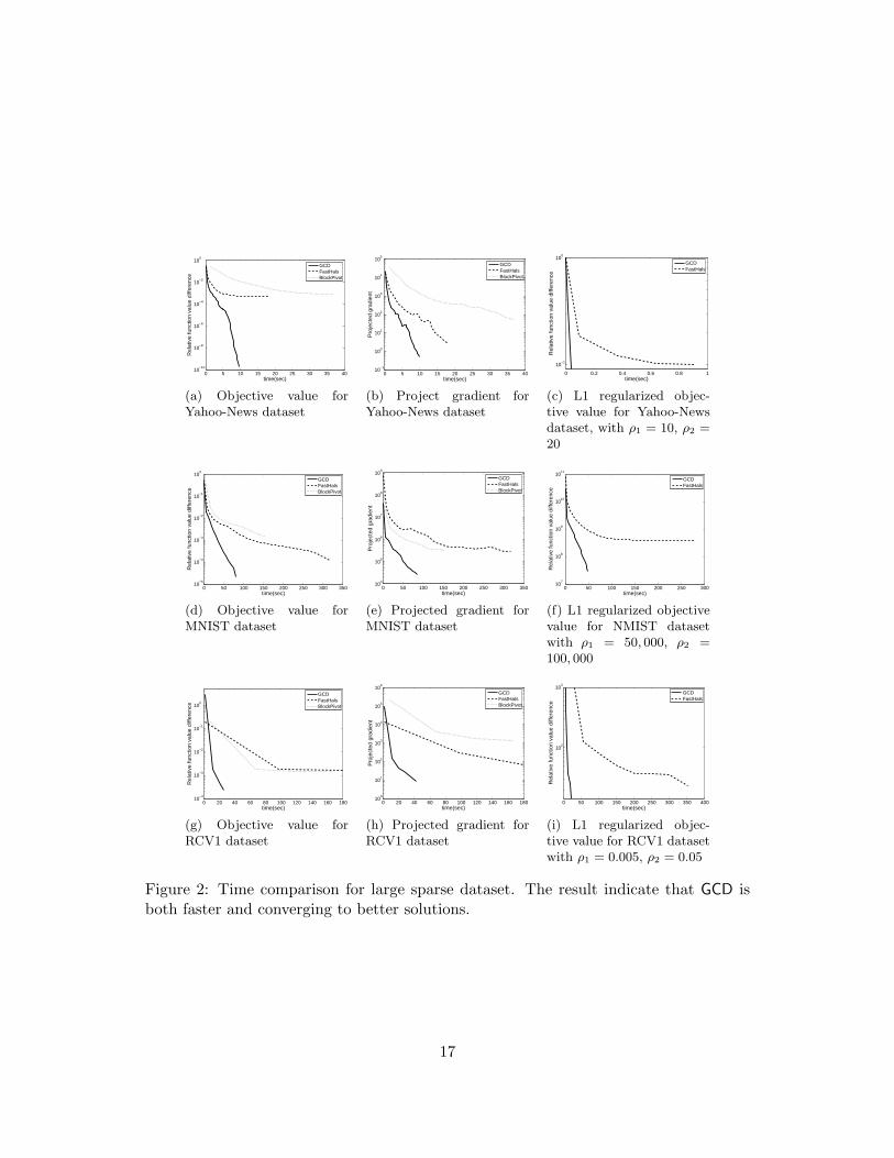
In Figure 2(a), 2(b), 2(c), we show the CPU time for the 3 methods to reduce theobjective value of least squares NMF, versus with logarithmically decreasing values of(f(W, H) − f∗)/f∗, where f∗ denote the lowest average objective value, for 10 initialpoints, of the 3 methods.

Compared to FastHals and BlockPivot, GCD converges to a local optimum with lowerobjective value. This is important for nonconvex optimization problems because we canfind a better local optimum. To further compare the speed of convergence to localoptimums, we check the projected gradient ∇P f(W, H), which measures the distancebetween current solution and stationary points. The results are in Figure 2(b), 2(e) and2(h). The figures indicate that GCD converges to the stationary point in lesser CPUtime.

We further add L1 penalty terms as in (2). We only include GCD and FastHals inthe comparison because BlockPivot does not provide the same regularized form in their

16

0 5 10 15 20 25 30 35 4010

−10

10−8

10−6

10−4

10−2

100

time(sec)

Rel

ativ

e fu

nctio

n va

lue

diffe

renc

e

GCDFastHalsBlockPivot

(a) Objective value forYahoo-News dataset

0 5 10 15 20 25 30 35 4010

−1

100

101

102

103

104

105

time(sec)

Pro

ject

ed g

radi

ent

GCDFastHalsBlockPivot

(b) Project gradient forYahoo-News dataset

0 0.2 0.4 0.6 0.8 1

10−1

100

time(sec)

Rel

ativ

e fu

nctio

n va

lue

diffe

renc

e

GCDFastHals

(c) L1 regularized objec-tive value for Yahoo-Newsdataset, with ρ1 = 10, ρ2 =20

0 50 100 150 200 250 300 35010

−5

10−4

10−3

10−2

10−1

100

time(sec)

Rel

ativ

e fu

nctio

n va

lue

diffe

renc

e

GCDFastHalsBlockPivot

(d) Objective value forMNIST dataset

0 50 100 150 200 250 300 35010

4

105

106

107

108

109

time(sec)

Pro

ject

ed g

radi

ent

GCDFastHalsBlockPivot

(e) Projected gradient forMNIST dataset

0 50 100 150 200 250 30010

7

108

109

1010

1011

time(sec)

Rel

ativ

e fu

nctio

n va

lue

diffe

renc

e

GCDFastHals

(f) L1 regularized objectivevalue for NMIST datasetwith ρ1 = 50, 000, ρ2 =100, 000

0 20 40 60 80 100 120 140 160 18010

−4

10−3

10−2

10−1

100

time(sec)

Rel

ativ

e fu

nctio

n va

lue

diffe

renc

e

GCDFastHalsBlockPivot

(g) Objective value forRCV1 dataset

0 20 40 60 80 100 120 140 160 18010

0

101

102

103

104

105

106

time(sec)

Pro

ject

ed g

radi

ent

GCDFastHalsBlockPivot

(h) Projected gradient forRCV1 dataset

0 50 100 150 200 250 300 350 400

102

103

time(sec)

Rel

ativ

e fu

nctio

n va

lue

diffe

renc

e

GCDFastHals

(i) L1 regularized objec-tive value for RCV1 datasetwith ρ1 = 0.005, ρ2 = 0.05

Figure 2: Time comparison for large sparse dataset. The result indicate that GCD isboth faster and converging to better solutions.

17

package. Figures 2(c), 2(f) and 2(i) compare the methods for reducing the objectivevalue of (2). For this comparison we choose the parameters λ1 and λ2 so that on averagemore than half variables in the solution of W and H are zero. The figures indicate thatGCD achieves lower objective value than FastHals in MNIST, and for Yahoo-News andRCV1, GCD is more than 10 times faster. This is because GCD can focus on nonzerovariables while FastHals updates all the variables at each iteration.

7 Discussion and Conclusions

In summary, we propose coordinate descent methods for solving least squares NMFand KL-NMF. Our methods have theoretical guarantees and efficient in solving realdata. The significant speedup in sparse data show a potential to apply NMF to largerproblems. In the future, our method can be extended to solve NMF with missing valuesor other matrix completion problems.

18

References

[1] M. Berry, M. Browne, A. Langville, P. Pauca, and R. Plemmon. Algorithms and ap-plications for approximate nonnegative matrix factorization. Computational Statis-tics and Data Analysis, 2007. Submitted.

[2] D. Bersekas and J. Tsitsiklis. Parallel and distributed computation. Prentice-Hall,1989.

[3] A. Cichocki and A.-H. Phan. Fast local algorithms for large scale nonnegative ma-trix and tensor factorizations. IEICE Transaction on Fundamentals, E92-A(3):708–721, 2009.

[4] E. Gaussier and C. Goutte. Relation between plsa and nmf and implications. 28thAnnual International ACM SIGIR Conference, 2005.

[5] E. F. Gonzales and Y. Zhang. Accelerating the Lee-Seung algorithm for non-negative matrix factorization. Technical report, Department of Computationaland Applied Mathematics, Rice University, 2005.

[6] L. Grippo and M. Sciandrone. On the convergence of the block nonlinear Gauss-Seidel method under convex constraints. Operations Research Letters, 26:127–136,2000.

[7] P. O. Hoyer. Non-negative sparse coding. In Proceedings of IEEE Workshop onNeural Networks for Signal Processing, pages 557–565, 2002.

[8] P. O. Hoyer. Non-negative matrix factorization with sparseness constraints. Journalof Machine Learning Research, 5:1457–1469, 2004.

[9] D. Kim, S. Sra, and I. S. Dhillon. Fast Newton-type methods for the least squaresnonnegative matrix appoximation problem. Proceedings of the Sixth SIAM Inter-national Conference on Data Mining, pages 343–354, 2007.

[10] J. Kim and H. Park. Non-negative matrix factorization based on alternating non-negativity constrained least squares and active set method. SIAM Journal onMatrix Analysis and Applications, 30(2):713–730, 2008.

[11] J. Kim and H. Park. Toward faster nonnegative matrix factorization: A newalgorithm and comparisons. Proceedings of the IEEE International Conference onData Mining, pages 353–362, 2008.

[12] Y. LeCun, L. Bottou, Y. Bengio, and P. Haffner. Gradient-based learning appliedto document recognition. Proceedings of the IEEE, 86(11):2278–2324, November1998. MNIST database available at http://yann.lecun.com/exdb/mnist/.

[13] D. D. Lee and H. S. Seung. Learning the parts of objects by non-negative matrixfactorization. Nature, 401:788–791, 1999.

19

[14] D. D. Lee and H. S. Seung. Algorithms for non-negative matrix factorization. InT. K. Leen, T. G. Dietterich, and V. Tresp, editors, Advances in Neural InformationProcessing Systems 13, pages 556–562. MIT Press, 2001.

[15] D. D. Lewis, Y. Yang, T. G. Rose, and F. Li. RCV1: A new benchmark collectionfor text categorization research. Journal of Machine Learning Research, 5:361–397,2004.

[16] C.-J. Lin. Projected gradient methods for non-negative matrix factorization. NeuralComputation, 19:2756–2779, 2007.

[17] C. Liu, H. chih Yang, J. Fan, L.-W. He, and Y.-M. Wang. Distributed Non-negativeMatrix Factorization for Web-Scale Dyadic Data Analysis on MapReduce. 2010.

[18] P. Paatero and U. Tapper. Positive matrix factorization: A non-negative factormodel with optimal utilization of error. Environmetrics, 5:111–126, 1994.

[19] J. Piper, P. Pauca, R. Plemmons, and M. Giffin. Object characterization from spec-tral data using nonnegative factorization and information theory. In Proceedingsof AMOS Technical Conference, 2004.

[20] R. Zdunek and A. Cichocki. Non-negative matrix factorization with quasi-newtonoptimization. Eighth International Conference on Artificial Intelligence and SoftComputing, ICAISC, pages 870–879, 2006.

20

8 Appendix

8.1 Lemma 1

Lemma 1 Assume GCD generates a sequence of (W, H) pairs:

(W 1, H1), (W 2, H1), (W 2, H2), . . . (27)

Suppose there exists a limit point (W , H). Then the function value globally convergesto some value:

limk→∞

f(W k, Hk) = limk→∞

f(W k+1, Hk) = f(W , H). (28)

Proof. This can be simply proved by the fact that our algorithm monotonicallydecreases the function value.

8.2 Proof of Theorem 1

Assume the Newton method generates the following sequence:

xi+1 = max(0, xi −f ′(xi)

f ′′(xi)), i = 0, 1, . . . (29)

The gradient and the second derivative are:

f ′(x) = −∑

i

cibi

ai + bix+ (

∑

i

bi)x (30)

f ′′(x) =∑

i

cib2i

(ai + bix)2> 0 (31)

First, we show thatf ′(xi) ≤ 0 ∀i ≥ 1. (32)

To prove (32), since f ′′(x) is positive and decreasing,

f ′(y) ≤ f ′(x) + (y − x)f ′′(x) ∀x, y ≥ 0.

By setting y = x − f ′(x)f ′′(x) we have

f ′(x −f ′(x)

f ′′(x)) ≤ 0.

Moreover, from (30) we have f ′(0) < 0. Therefore after one Newton step, xi+1 will

be either xi − f ′(xi)f ′′(xi)

or 0. In either case (32) holds. Therefore the sequence after the

first iteration {xi}i≥1 have the property that f ′(xi) < 0 and, thus − f ′(xi)f ′′(xi)

> 0. So the

sequence {xi}i≥1 is monotonically increasing in a compact set f ′(x) ≤ 0. {xi} then

21

converges to a limit point, say x∗. f ′(x∗) can be either negative or zero. If f ′(x∗) < 0,since limi→∞ xi = x∗, when i is large enough we have the following two properties bycontinuity of first and second derivatives:

f ′(xi)

f ′′(xi)<

f ′(x∗)

2f ′′(x∗)(33)

x∗ − xi < −f ′(x∗)

2f ′′(x∗)(34)

Combine (33) and (34) we have

x∗ − xi+1 = x∗ − xi +f ′(xi)

f ′′(xi)< 0,

which raises the contradiction with xi+1 ≤ x∗. So the Newton method converges to theoptimal solution f ′(x∗) = 0.

8.3 Proof of Theorem 2

First, we look into our algorithm to see what properties we can use. In a sequence ofupdates from (W k, Hk) to (W k+1, Hk), at the beginning GCD computes the maximumfunction value reduction for one coordinate:

v0 = maxi,j,q:W k

ij+q≥0f(W k, Hk) − f(W k + qeij , H

k).

From Section 2, GCD will choose this variable with objective function decreasing v0 nomatter selecting the max element in DW or selecting max value row by row. So we have

f(W k, Hk) − f(W k+1, Hk) ≥ v0. (35)

GCD updates variables in W until the maximum possible function value reduction isless than ǫv0, that is, in the end of updates of variables of W , we will get W k+1 withthe following property:

maxi,j,q:W k+1

ij +q≥0f(W k+1, Hk) − f(W k+1 + qeij , H

k) < ǫv0 ≤ v0, (36)

where ǫ ∈ (0, 1). Combining (35) and (36)

f(W k, Hk) − f(W k+1, Hk) >

maxi,j,q:W k+1

ij +q≥0f(W k+1, Hk) − f(W k+1 + qeij , H

k). (37)

We will use (37) for later proof.

22

For a sequence of updates on variables of H, assume at the beginning the maximumfunction value decreasing is

v0 = maxi,j,p:Hk

ij+p≥0f(W k+1, Hk) − f(W k+1, Hk + peij)

= f(W k+1, Hk) − mini,j,p:Hk

ij+p≥0f(W k+1, Hk + peij) (38)

By the same argument of (35), we have

f(W k+1, Hk) − f(W k+1, Hk+1) ≥ v0. (39)

With (38) we have

f(W k+1, Hk+1) ≤ mini,j,p:Hk

ij+p≥0f(W k+1, Hk + peij). (40)

Next we will use (37) and (40) to finish our proof. Assume the sequence has a limitpoint (W , H), without loss of generality, assume there is a subsequence

{W k+1, Hk}k∈K → (W , H), (41)

(otherwise there will exist {W k, Hk} → (W , H), and we can use the similar argument.)Now if (W , H) is not a stationary point, one of the following conditions will hold:

∃i, j, q such that f(W + qeij , H) ≤ f(W , H) − σ (42)

∃i, j, p such that f(W , H + peij) ≤ f(W , H) − σ (43)

for some σ > 0.First, consider when (42) happens for some i, j and q. From the continuity of f(·)

we know there exists a large enough constant R such that

f(W k+1 + peij , Hk) ≤ f(W , H) − σ/2 ∀k > R and k ∈ K

Thus

f(W k+1, Hk) − f(W k+1 + peij , Hk) ≥

f(W k+1, Hk) − f(W , H) + σ/2 ≥ σ/2,

where the second inequality comes from the monotonicity of the sequence generated byGCD. With (37) we have

f(W k, Hk) − f(W k+1, Hk) > σ/2 ∀k > R and k ∈ K.

However, this will make f(W k, Hk) → −∞ when k → ∞, a contradiction.Second, when case (43) happens, by (40) we have

f(W k+1, Hk+1) ≤ f(W k+1, Hk + qeij) < f(W k+1, Hk)

23

when k large enough. By the continuity of f and the fact that limk∈K(W k+1, Hk) =(W , H), taking limit on both sides and using Lemma 1, we get

f(W , H + qeij) = f(W , H),

which raises the contradiction with (43).Since both case (42) and (43) cannot happen, any limit point of our algorithm is a

stationary point.

24