Embed Size (px)
Citation preview

Motivation APPROX Accelerated Parallel Proximal Numerical results
Accelerated, Parallel and ProximalCoordinate Descent
Olivier Fercoq
Joint work with P. Richtarik
22 June 2015
17th Leslie Fox Prize competition
1/29
Motivation APPROX Accelerated Parallel Proximal Numerical results
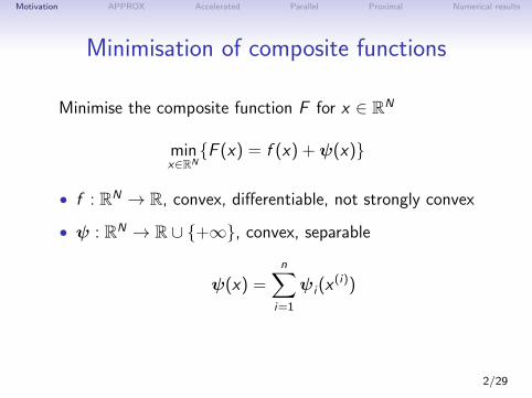
Minimisation of composite functions
Minimise the composite function F for x ∈ RN
minx∈RN{F (x) = f (x) +ψ(x)}
• f : RN → R, convex, differentiable, not strongly convex
• ψ : RN → R ∪ {+∞}, convex, separable
ψ(x) =n∑
i=1
ψi(x(i))
2/29
Motivation APPROX Accelerated Parallel Proximal Numerical results
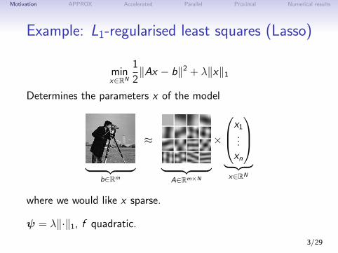
Example: L1-regularised least squares (Lasso)
minx∈RN
1
2‖Ax − b‖2 + λ‖x‖1
Determines the parameters x of the model
︸ ︷︷ ︸b∈Rm
≈
︸ ︷︷ ︸A∈Rm×N
×
x1...xn
︸ ︷︷ ︸x∈RN
where we would like x sparse.
ψ = λ‖·‖1, f quadratic.
3/29
Motivation APPROX Accelerated Parallel Proximal Numerical results
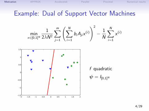
Example: Dual of Support Vector Machines
minx∈[0,1]N
1
2λN2
m∑j=1
(N∑i=1
biAjix(i)
)2
− 1
N
N∑i=1
x (i)
−2 −1.5 −1 −0.5 0 0.5 1 1.5 2−1.5
−1
−0.5
0
0.5
1
1.5
f quadratic
ψ = I[0,1]N
4/29
Motivation APPROX Accelerated Parallel Proximal Numerical results
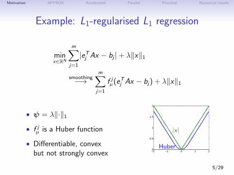
Example: L1-regularised L1 regression
minx∈RN
m∑j=1
|eTj Ax − bj |+ λ‖x‖1
smoothing−→m∑j=1
f jµ(eTj Ax − bj) + λ‖x‖1
• ψ = λ‖·‖1
• f jµ is a Huber function
• Differentiable, convexbut not strongly convex −2 −1 0 1 2
0
0.5
1
1.5
2
|x |
Huber
5/29
Motivation APPROX Accelerated Parallel Proximal Numerical results
Coordinate descentf has Lipschitz continuous directional derivatives:
f (x + tei) ≤ f (x) + 〈∇f (x), tei〉+Li2‖tei‖2
At each iteration:
1. Choose randomly a coordinate i2. Compute the update t ∈ R that minimises
the overapproximation of f (x + tei)3. Update the variable x ← x + tei
Remarks:
• Many iterations are needed• Each iteration is cheap• Well fitted to sparse matrices in column format
6/29
Motivation APPROX Accelerated Parallel Proximal Numerical results
Proximal coordinate descentF = f +ψ:
F (x + tei) ≤ ψ(x + tei) + f (x) + 〈∇f (x), tei〉+Li2‖tei‖2
At each iteration:
1. Choose randomly a coordinate i2. Compute the update t ∈ R that minimises
the overapproximation of F (x + tei)3. Update the variable x ← x + tei
Remarks:• Essential to deal with non-smooth regularisers• Involves the proximity operator of ψi : proxψi
Ex: projection onto a box, soft thresholding• Adding separable ψ : same speed of convergence
7/29
Motivation APPROX Accelerated Parallel Proximal Numerical results
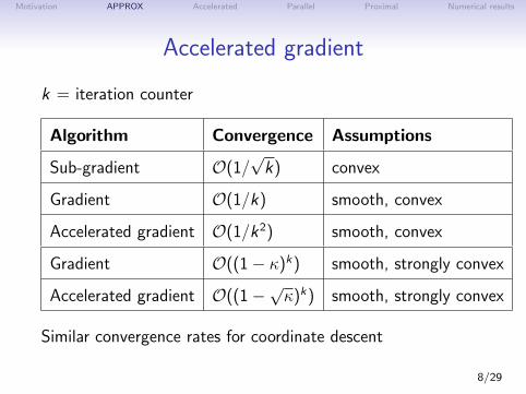
Accelerated gradient
k = iteration counter
Algorithm Convergence Assumptions
Sub-gradient O(1/√k) convex
Gradient O(1/k) smooth, convex
Accelerated gradient O(1/k2) smooth, convex
Gradient O((1− κ)k) smooth, strongly convex
Accelerated gradient O((1−√κ)k) smooth, strongly convex
Similar convergence rates for coordinate descent
8/29
Motivation APPROX Accelerated Parallel Proximal Numerical results
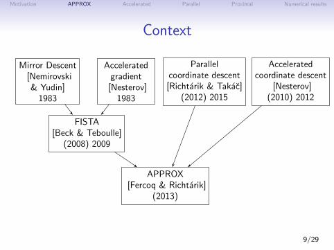
Context
APPROX[Fercoq & Richtarik]
(2013)
FISTA[Beck & Teboulle]
(2008) 2009
Acceleratedgradient
[Nesterov]1983
Mirror Descent[Nemirovski& Yudin]
1983
Parallelcoordinate descent[Richtarik & Takac]
(2012) 2015
Acceleratedcoordinate descent
[Nesterov](2010) 2012
9/29
Motivation APPROX Accelerated Parallel Proximal Numerical results
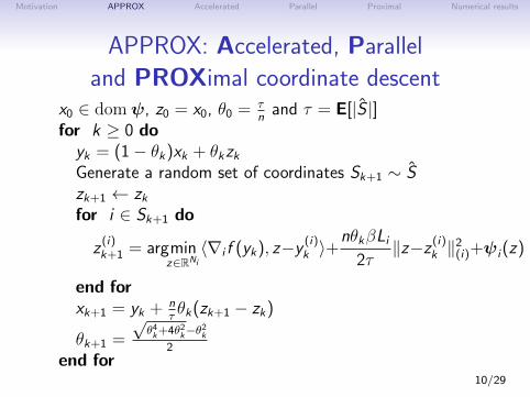
APPROX: Accelerated, Parallel
and PROXimal coordinate descentx0 ∈ domψ, z0 = x0, θ0 = τ
nand τ = E[|S |]
for k ≥ 0 doyk = (1− θk)xk + θkzkGenerate a random set of coordinates Sk+1 ∼ Szk+1 ← zkfor i ∈ Sk+1 do
z(i)k+1 = argmin
z∈RNi
〈∇i f (yk), z−y (i)k 〉+
nθkβLi2τ
‖z−z (i)k ‖2(i)+ψi(z)
end forxk+1 = yk + n
τθk(zk+1 − zk)
θk+1 =
√θ4k+4θ2k−θ
2k
2
end for10/29
Motivation APPROX Accelerated Parallel Proximal Numerical results
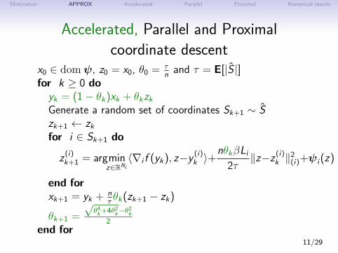
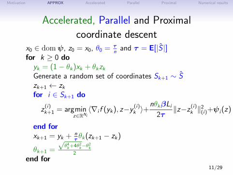
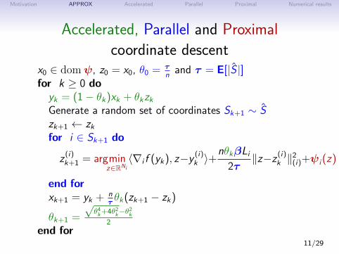
Accelerated, Parallel and Proximal
coordinate descentx0 ∈ domψ, z0 = x0, θ0 = τ
nand τ = E[|S |]
for k ≥ 0 doyk = (1− θk)xk + θkzkGenerate a random set of coordinates Sk+1 ∼ Szk+1 ← zkfor i ∈ Sk+1 do
z(i)k+1 = argmin
z∈RNi
〈∇i f (yk), z−y (i)k 〉+
nθkβLi2τ
‖z−z (i)k ‖2(i)+ψi(z)
end forxk+1 = yk + n
τθk(zk+1 − zk)
θk+1 =
√θ4k+4θ2k−θ
2k
2
end for11/29
Motivation APPROX Accelerated Parallel Proximal Numerical results
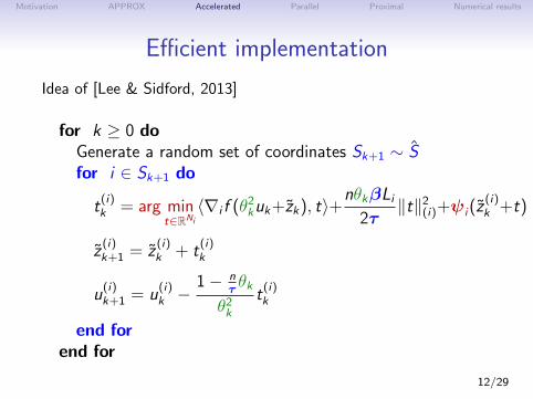
Efficient implementation
Idea of [Lee & Sidford, 2013]
for k ≥ 0 doGenerate a random set of coordinates Sk+1 ∼ Sfor i ∈ Sk+1 do
t(i)k = arg min
t∈RNi
〈∇i f (θ2kuk+zk), t〉+nθkβLi2τ
‖t‖2(i)+ψi(z(i)k +t)
z(i)k+1 = z
(i)k + t
(i)k
u(i)k+1 = u
(i)k −
1− nτθk
θ2kt(i)k
end forend for
12/29
Motivation APPROX Accelerated Parallel Proximal Numerical results
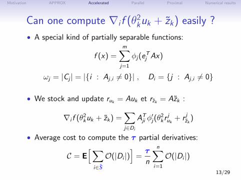
Can one compute ∇i f (θ2kuk + zk) easily ?
• A special kind of partially separable functions:
f (x) =m∑j=1
φj(eTj Ax)
ωj = |Cj | = |{i : Aj ,i 6= 0}| , Di = {j : Aj ,i 6= 0}
• We stock and update ruk = Auk et rzk = Azk :
∇i f (θ2kuk + zk) =∑j∈Di
ATji φ′j(θ
2kr
juk
+ r jzk )
• Average cost to compute the τ partial derivatives:
C = E[∑
i∈S
O(|Di |)]
=τ
n
n∑i=1
O(|Di |)
13/29
Motivation APPROX Accelerated Parallel Proximal Numerical results
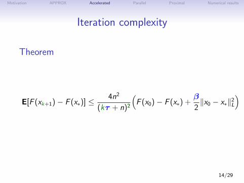
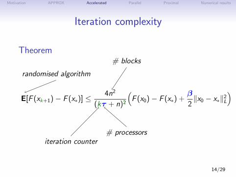
Iteration complexity
Theorem
E[F (xk+1)− F (x∗)] ≤ 4n2
(kτ + n)2
(F (x0)− F (x∗) +
β
2‖x0 − x∗‖2L
)
randomised algorithm
# blocks
iteration counter# processors
depends of τ
14/29
Motivation APPROX Accelerated Parallel Proximal Numerical results
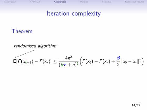
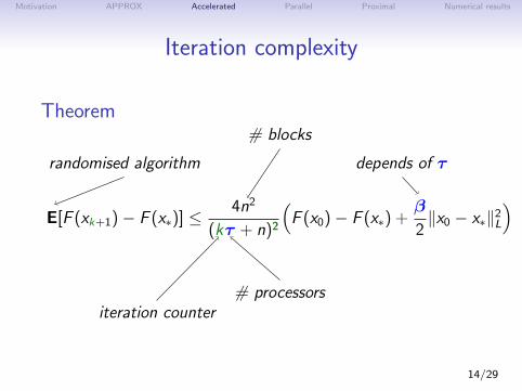
Iteration complexity
Theorem
E[F (xk+1)− F (x∗)] ≤ 4n2
(kτ + n)2
(F (x0)− F (x∗) +
β
2‖x0 − x∗‖2L
)randomised algorithm
# blocks
iteration counter# processors
depends of τ
14/29
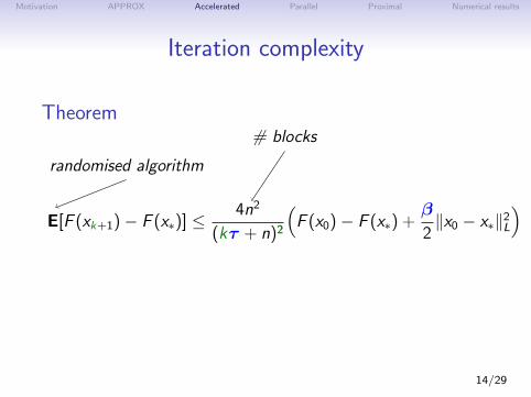
Motivation APPROX Accelerated Parallel Proximal Numerical results
Iteration complexity
Theorem
E[F (xk+1)− F (x∗)] ≤ 4n2
(kτ + n)2
(F (x0)− F (x∗) +
β
2‖x0 − x∗‖2L
)randomised algorithm
# blocks
iteration counter# processors
depends of τ
14/29
Motivation APPROX Accelerated Parallel Proximal Numerical results
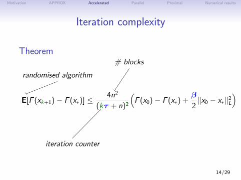
Iteration complexity
Theorem
E[F (xk+1)− F (x∗)] ≤ 4n2
(kτ + n)2
(F (x0)− F (x∗) +
β
2‖x0 − x∗‖2L
)randomised algorithm
# blocks
iteration counter
# processors
depends of τ
14/29
Motivation APPROX Accelerated Parallel Proximal Numerical results
Iteration complexity
Theorem
E[F (xk+1)− F (x∗)] ≤ 4n2
(kτ + n)2
(F (x0)− F (x∗) +
β
2‖x0 − x∗‖2L
)randomised algorithm
# blocks
iteration counter# processors
depends of τ
14/29
Motivation APPROX Accelerated Parallel Proximal Numerical results
Iteration complexity
Theorem
E[F (xk+1)− F (x∗)] ≤ 4n2
(kτ + n)2
(F (x0)− F (x∗) +
β
2‖x0 − x∗‖2L
)randomised algorithm
# blocks
iteration counter# processors
depends of τ
14/29
Motivation APPROX Accelerated Parallel Proximal Numerical results
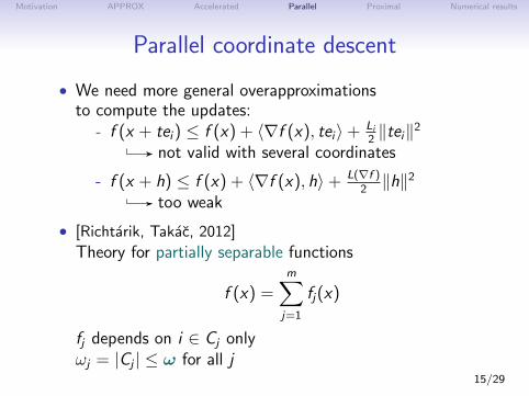
Parallel coordinate descent
• We need more general overapproximationsto compute the updates:
- f (x + tei) ≤ f (x) + 〈∇f (x), tei〉+ Li2‖tei‖2
not valid with several coordinates
- f (x + h) ≤ f (x) + 〈∇f (x), h〉+ L(∇f )2‖h‖2
too weak
• [Richtarik, Takac, 2012]
Theory for partially separable functions
f (x) =m∑j=1
fj(x)
fj depends on i ∈ Cj onlyωj = |Cj | ≤ ω for all j
15/29
Motivation APPROX Accelerated Parallel Proximal Numerical results
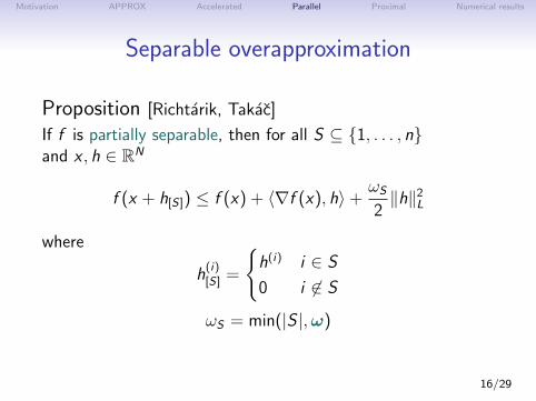
Separable overapproximation
Proposition [Richtarik, Takac]
If f is partially separable, then for all S ⊆ {1, . . . , n}and x , h ∈ RN
f (x + h[S]) ≤ f (x) + 〈∇f (x), h〉+ωS
2‖h‖2L
where
h(i)[S] =
{h(i) i ∈ S
0 i 6∈ S
ωS = min(|S |,ω)
16/29
Motivation APPROX Accelerated Parallel Proximal Numerical results
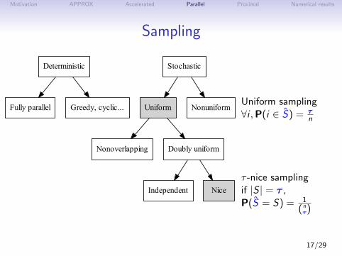
Sampling
Deterministic
Fully parallel Greedy, cyclic...
Stochastic
Uniform Nonuniform
Nonoverlapping Doubly uniform
Independent Nice
Uniform sampling∀i ,P(i ∈ S) = τ
n
τ -nice samplingif |S | = τ ,P(S = S) = 1
(nτ)
17/29
Motivation APPROX Accelerated Parallel Proximal Numerical results
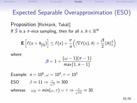
Expected Separable Overapproximation (ESO)
Proposition [Richtarik, Takac]
If S is a τ -nice sampling, then for all x , h ∈ RN
E[f (x + h[S])
]≤ f (x) +
τ
n
(〈∇f (x), h〉+
β
2‖h‖2L
)where
β = 1 +(ω − 1)(τ − 1)
max{1, n − 1}
Example: n = 106, ω = 104, τ = 103
ESO β ≈ 11⇒ τ√β≈ 300
whereas ωS = min(ω, τ) = τ ⇒ τ√ωS≈ 30
18/29
Motivation APPROX Accelerated Parallel Proximal Numerical results
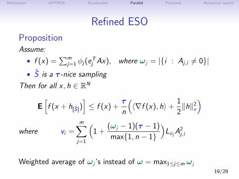
Refined ESO
PropositionAssume:
• f (x) =∑m
j=1 φj(eTj Ax), where ωj = |{i : Aj ,i 6= 0}|
• S is a τ -nice sampling
Then for all x , h ∈ RN
E[f (x + h[S])
]≤ f (x) +
τ
n
(〈∇f (x), h〉+
1
2‖h‖2v
)where vi =
m∑j=1
(1 +
(ωj − 1)(τ − 1)
max{1, n − 1}
)LφjA
2j ,i
Weighted average of ωj ’s instead of ω = max1≤j≤m ωj
19/29
Motivation APPROX Accelerated Parallel Proximal Numerical results
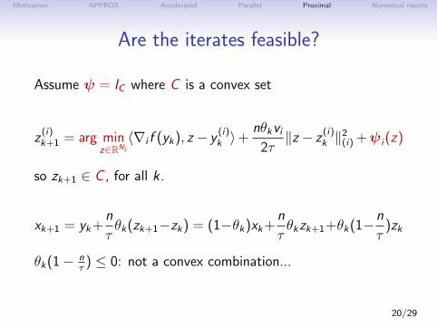
Are the iterates feasible?
Assume ψ = IC where C is a convex set
z(i)k+1 = arg min
z∈RNi
〈∇i f (yk), z − y(i)k 〉+
nθkvi2τ‖z − z
(i)k ‖
2(i) +ψi(z)
so zk+1 ∈ C , for all k .
xk+1 = yk+n
τθk(zk+1−zk) = (1−θk)xk+
n
τθkzk+1+θk(1−n
τ)zk
θk(1− nτ
) ≤ 0: not a convex combination...
20/29
Motivation APPROX Accelerated Parallel Proximal Numerical results
Feasibility
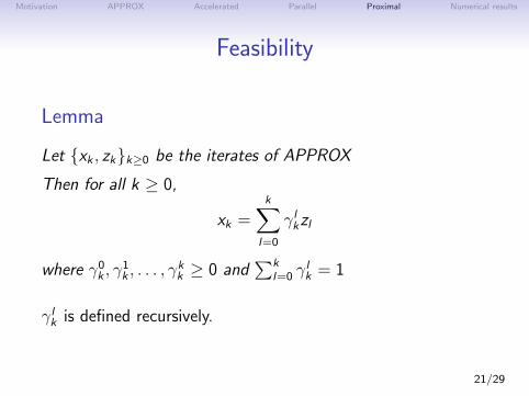
Lemma
Let {xk , zk}k≥0 be the iterates of APPROX
Then for all k ≥ 0,
xk =k∑
l=0
γ lkzl
where γ0k , γ1k , . . . , γ
kk ≥ 0 and
∑kl=0 γ
lk = 1
γ lk is defined recursively.
21/29

Motivation APPROX Accelerated Parallel Proximal Numerical results
Supermartingale inequality
Define: Fk =f (xk) +k∑
l=0
γ lkψ(zl) ≥ F (xk)
Then
E[1− θk+1
θk+12
(Fk+1−F (x∗)) +βn2
2τ 2‖x∗ − zk+1‖2L
∣∣ Sk+1
]≤ 1− θk
θk2(Fk − F (x∗)) +
βn2
2τ 2‖x∗ − zk‖2L
22/29
Motivation APPROX Accelerated Parallel Proximal Numerical results
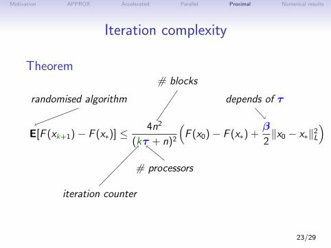
Iteration complexity
Theorem
E[F (xk+1)− F (x∗)] ≤ 4n2
(kτ + n)2
(F (x0)− F (x∗) +
β
2‖x0 − x∗‖2L
)randomised algorithm
# blocks
iteration counter
# processors
depends of τ
23/29
Motivation APPROX Accelerated Parallel Proximal Numerical results
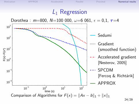
L1 RegressionDorothea : m=800, N=100 000, ω=6 061, ε = 0,1, τ=4
10−1
100
101
102
10−2
10−1
100
101
102
103
time (s)
F(x
)−F
(x*)
Sedumi
Gradient(smoothed function)
Accelerated gradient[Nesterov, 2005]
SPCDM[Fercoq & Richtarik]
APPROX
Comparison of Algorithms for F (x) = ‖Ax − b‖1 + ‖x‖124/29
Motivation APPROX Accelerated Parallel Proximal Numerical results
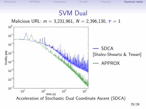
SVM DualMalicious URL: m = 3,231,961, N = 2,396,130, τ = 1
101
102
103
104
10−7
10−6
10−5
10−4
10−3
10−2
10−1
100
time (s)
Dua
lity
gap
SDCA[Shalev-Shwartz & Tewari]
APPROX
Acceleration of Stochastic Dual Coordinate Ascent (SDCA)
25/29
Motivation APPROX Accelerated Parallel Proximal Numerical results
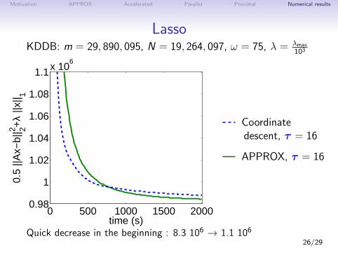
LassoKDDB: m = 29, 890, 095, N = 19, 264, 097, ω = 75, λ = λmax
103
0 500 1000 1500 20000.98
1
1.02
1.04
1.06
1.08
1.1x 10⁶
time (s)
0.5
||Ax−
b||2 2+
λ ||x
|| 1
Coordinatedescent, τ = 16
APPROX, τ = 16
Quick decrease in the beginning : 8.3 106 → 1.1 10626/29
Motivation APPROX Accelerated Parallel Proximal Numerical results
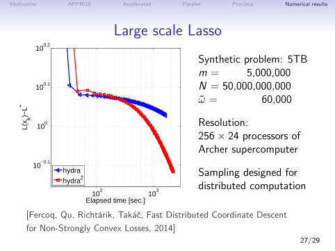
Large scale Lasso
102
103
10−0.1
100
100.1
100.2
Elapsed time [sec.]
L(x k)−
L*
hydra
hydra2
Synthetic problem: 5TBm = 5,000,000N = 50,000,000,000ω = 60,000
Resolution:256× 24 processors ofArcher supercomputer
Sampling designed fordistributed computation
[Fercoq, Qu, Richtarik, Takac, Fast Distributed Coordinate Descent
for Non-Strongly Convex Losses, 2014]27/29
Motivation APPROX Accelerated Parallel Proximal Numerical results
Extensions
Nearly 50 citations:
[Qu, Richtarik, 2014]Fixed non-uniform samplings
[Allen-Zhu, Orecchia, 2014]Large scale continuous packing LP
[Lin, Lu, Xiao, 2014]Strongly convex functions and primal-dual method
[Ene, Nguyen, 2015]Restarting and minimisation of submodular functions
[Sun, Toh, Yang, 2015]Least squares semidefinite programming
28/29
Motivation APPROX Accelerated Parallel Proximal Numerical results
Conclusion
• Summary
- 1st accelerated, parallel and proximal coordinatedescent method
- Improved step sizes for parallel coordinate descent
- Versatile algorithm, efficient for large scale problems
• Perspectives
- Relax the i.i.d. sampling assumption
- Primal-dual algorithm (non-separable & non-smooth)
- Accelerating stochastic averaged gradient
29/29