Fast and Unambiguous Direction Finding for Digital Radar ...€¦ · Fast and Unambiguous Direction Finding for Digital Radar Intercept Receivers Peter Quoc Cuong Ly A Thesis Submitted

Fast and UnambiguousDirection Finding for Digital

Radar Intercept Receivers

Peter Quoc Cuong Ly

A Thesis Submitted for the Degree of

Doctor of Philosophy

School of Electrical and Electronic EngineeringThe University of AdelaideAdelaide, South Australia

December 2013

For my wife, Joy

The Light of my Life

Contents

List of Figures v

List of Tables xiii

Abstract xv

Declaration xvii

Acknowledgements xix

Publications xxi

Acronyms xxiii

Notation xxv

1 Introduction 11.1 Introduction . . . . . . . . . . . . . . . . . . . . . . . . . . . . . . . . . . 11.2 Electronic Support . . . . . . . . . . . . . . . . . . . . . . . . . . . . . . 11.3 The Importance of Direction Finding . . . . . . . . . . . . . . . . . . . . 3

1.3.1 Situational Awareness . . . . . . . . . . . . . . . . . . . . . . . . 31.3.2 Signal Deinterleaving . . . . . . . . . . . . . . . . . . . . . . . . . 31.3.3 Electronic Attack and Electronic Protection Measures . . . . . . 41.3.4 Signal Enhancement . . . . . . . . . . . . . . . . . . . . . . . . . 41.3.5 Beaming Manoeuvre . . . . . . . . . . . . . . . . . . . . . . . . . 4

1.4 Problem Statement . . . . . . . . . . . . . . . . . . . . . . . . . . . . . . 51.4.1 Design Constraints of a Radar Intercept Receiver . . . . . . . . . 51.4.2 One-Way Propagation Advantage . . . . . . . . . . . . . . . . . . 61.4.3 Implications for AOA Estimation . . . . . . . . . . . . . . . . . . 71.4.4 Assumptions . . . . . . . . . . . . . . . . . . . . . . . . . . . . . 8

1.5 Organisation of this Thesis . . . . . . . . . . . . . . . . . . . . . . . . . 101.6 Original Contributions . . . . . . . . . . . . . . . . . . . . . . . . . . . . 12

2 Contemporary Direction Finding Techniques 132.1 Spinning Antenna . . . . . . . . . . . . . . . . . . . . . . . . . . . . . . 132.2 Amplitude Comparison . . . . . . . . . . . . . . . . . . . . . . . . . . . 14

2.2.1 Loop Antennas . . . . . . . . . . . . . . . . . . . . . . . . . . . . 152.2.2 Adcock Arrays . . . . . . . . . . . . . . . . . . . . . . . . . . . . 152.2.3 Cavity-Backed Spiral Antennas . . . . . . . . . . . . . . . . . . . 16

i

CONTENTS ii

2.3 Frequency-Difference-of-Arrival . . . . . . . . . . . . . . . . . . . . . . . 182.4 Time-Difference-of-Arrival . . . . . . . . . . . . . . . . . . . . . . . . . . 192.5 Interferometry . . . . . . . . . . . . . . . . . . . . . . . . . . . . . . . . 202.6 Beamforming and Array Processing . . . . . . . . . . . . . . . . . . . . . 202.7 Summary . . . . . . . . . . . . . . . . . . . . . . . . . . . . . . . . . . . 22

3 Interferometry 253.1 Introduction . . . . . . . . . . . . . . . . . . . . . . . . . . . . . . . . . . 253.2 Signal Model . . . . . . . . . . . . . . . . . . . . . . . . . . . . . . . . . 25

3.2.1 Propagation Delays . . . . . . . . . . . . . . . . . . . . . . . . . 263.2.2 Narrowband Signal Model . . . . . . . . . . . . . . . . . . . . . . 28

3.3 Interferometry . . . . . . . . . . . . . . . . . . . . . . . . . . . . . . . . 293.3.1 Relationship to TDOA . . . . . . . . . . . . . . . . . . . . . . . . 29

3.4 AOA Estimation in the Presence of Receiver Noise . . . . . . . . . . . . 303.4.1 Maximum Likelihood Estimate . . . . . . . . . . . . . . . . . . . 303.4.2 Time-Domain Methods . . . . . . . . . . . . . . . . . . . . . . . 313.4.3 Cramer-Rao Lower Bound for a Two-Antenna Interferometer . . 323.4.4 Performance Comparison . . . . . . . . . . . . . . . . . . . . . . 333.4.5 RMS Error of an Interferometer . . . . . . . . . . . . . . . . . . 36

3.5 Long Baseline Interferometry . . . . . . . . . . . . . . . . . . . . . . . . 363.6 Ambiguity Resolution Using Independent Methods . . . . . . . . . . . . 42

3.6.1 Amplitude Comparison . . . . . . . . . . . . . . . . . . . . . . . 433.6.2 Short Baseline . . . . . . . . . . . . . . . . . . . . . . . . . . . . 43

3.7 Ambiguity Resolution Using Multiple Baselines . . . . . . . . . . . . . . 453.7.1 The Chinese Remainder Theorem . . . . . . . . . . . . . . . . . . 453.7.2 Non-Uniform Array Geometry . . . . . . . . . . . . . . . . . . . 523.7.3 Number of Baselines . . . . . . . . . . . . . . . . . . . . . . . . . 553.7.4 Maximum Likelihood Estimator . . . . . . . . . . . . . . . . . . 563.7.5 Correlative Interferometers . . . . . . . . . . . . . . . . . . . . . 583.7.6 Common Angle Search . . . . . . . . . . . . . . . . . . . . . . . . 603.7.7 Line Fitting . . . . . . . . . . . . . . . . . . . . . . . . . . . . . . 65

3.8 Performance Comparison . . . . . . . . . . . . . . . . . . . . . . . . . . 693.8.1 Cramer-Rao Lower Bound for a Non-Uniform Linear Array . . . 693.8.2 Array Geometry . . . . . . . . . . . . . . . . . . . . . . . . . . . 703.8.3 Monte Carlo Simulations . . . . . . . . . . . . . . . . . . . . . . 71

3.9 Other Considerations . . . . . . . . . . . . . . . . . . . . . . . . . . . . . 753.9.1 Multiple Signals . . . . . . . . . . . . . . . . . . . . . . . . . . . 753.9.2 Optimal Linear Array Geometries . . . . . . . . . . . . . . . . . 753.9.3 Field-of-View . . . . . . . . . . . . . . . . . . . . . . . . . . . . . 76

3.10 Summary . . . . . . . . . . . . . . . . . . . . . . . . . . . . . . . . . . . 80

4 Interferometry Using Second Order Difference Arrays 834.1 Introduction . . . . . . . . . . . . . . . . . . . . . . . . . . . . . . . . . . 834.2 SODA Interferometry . . . . . . . . . . . . . . . . . . . . . . . . . . . . 84

4.2.1 Unambiguous AOA Estimation . . . . . . . . . . . . . . . . . . . 844.2.2 Correction for Ambiguous Phase Delay Measurements . . . . . . 854.2.3 Algorithm Complexity . . . . . . . . . . . . . . . . . . . . . . . . 864.2.4 Alternate Expressions for the SODA Baseline Constraint . . . . 86

CONTENTS iii

4.2.5 RMS Error of the SODA Interferometer . . . . . . . . . . . . . . 874.2.6 Performance Evaluation . . . . . . . . . . . . . . . . . . . . . . . 89

4.3 SODA-Cued Ambiguity Resolution . . . . . . . . . . . . . . . . . . . . . 914.3.1 SODA-Based Inference (SBI) Interferometer . . . . . . . . . . . . 924.3.2 SODA-Cued Correlative Interferometer . . . . . . . . . . . . . . 934.3.3 SBI-Cued Correlative Interferometer . . . . . . . . . . . . . . . . 94

4.4 Performance Comparison . . . . . . . . . . . . . . . . . . . . . . . . . . 954.5 Other Considerations . . . . . . . . . . . . . . . . . . . . . . . . . . . . . 99

4.5.1 Other Linear Combinations of First-Order Phase Delays . . . . . 994.5.2 Non-Collinear SODA Interferometer . . . . . . . . . . . . . . . . 1014.5.3 Field-of-View . . . . . . . . . . . . . . . . . . . . . . . . . . . . . 103

4.6 Summary . . . . . . . . . . . . . . . . . . . . . . . . . . . . . . . . . . . 103

5 Array Processing Using Second Order Difference Arrays 1075.1 Beamforming and Array Processing . . . . . . . . . . . . . . . . . . . . . 107

5.1.1 Signal Model . . . . . . . . . . . . . . . . . . . . . . . . . . . . . 1075.1.2 Conventional Phaseshift Beamformer . . . . . . . . . . . . . . . . 1095.1.3 Optimal Beamformers and Super-Resolution Methods . . . . . . 1135.1.4 Multiple Signal Classification (MUSIC) . . . . . . . . . . . . . . 113

5.2 Sparse Large Aperture Arrays . . . . . . . . . . . . . . . . . . . . . . . . 1145.2.1 Grid Search Resolution . . . . . . . . . . . . . . . . . . . . . . . 118

5.3 Array Processing with SODA Geometries . . . . . . . . . . . . . . . . . 1245.3.1 SODA-Cued Array Processing . . . . . . . . . . . . . . . . . . . 1245.3.2 SBI-Cued Array Processing . . . . . . . . . . . . . . . . . . . . . 1265.3.3 SODA Array Processing . . . . . . . . . . . . . . . . . . . . . . . 127

5.4 Performance Comparison . . . . . . . . . . . . . . . . . . . . . . . . . . 1335.4.1 Array Beampatterns . . . . . . . . . . . . . . . . . . . . . . . . . 1335.4.2 Grid Search Resolutions . . . . . . . . . . . . . . . . . . . . . . . 1345.4.3 Monte Carlo Simulations . . . . . . . . . . . . . . . . . . . . . . 134

5.5 Summary . . . . . . . . . . . . . . . . . . . . . . . . . . . . . . . . . . . 141

6 Calibration 1436.1 Introduction . . . . . . . . . . . . . . . . . . . . . . . . . . . . . . . . . . 1436.2 Effect of Channel Imbalances . . . . . . . . . . . . . . . . . . . . . . . . 144

6.2.1 Phase, Frequency and Baseline Errors . . . . . . . . . . . . . . . 1446.2.2 Gain Imbalance . . . . . . . . . . . . . . . . . . . . . . . . . . . . 146

6.3 Signal Models . . . . . . . . . . . . . . . . . . . . . . . . . . . . . . . . . 1486.3.1 Calibrated Signal Model . . . . . . . . . . . . . . . . . . . . . . . 1486.3.2 Uncalibrated Signal Model . . . . . . . . . . . . . . . . . . . . . 149

6.4 Calibration Methodology . . . . . . . . . . . . . . . . . . . . . . . . . . . 1506.4.1 Calibration Tables . . . . . . . . . . . . . . . . . . . . . . . . . . 1506.4.2 Simple Calibration . . . . . . . . . . . . . . . . . . . . . . . . . . 1516.4.3 Joint Calibration and AOA Estimation . . . . . . . . . . . . . . 151

6.5 Short-Baseline Calibration . . . . . . . . . . . . . . . . . . . . . . . . . . 1516.5.1 Implementation Using a 1-D Look-Up-Table . . . . . . . . . . . . 156

6.6 Long-Baseline Calibration . . . . . . . . . . . . . . . . . . . . . . . . . . 1566.6.1 Ambiguity Resolution Using Multiple Baselines and Uncalibrated

Data . . . . . . . . . . . . . . . . . . . . . . . . . . . . . . . . . . 161

CONTENTS iv

6.7 Summary . . . . . . . . . . . . . . . . . . . . . . . . . . . . . . . . . . . 163

7 The Electronic Support Testbed 1657.1 Introduction . . . . . . . . . . . . . . . . . . . . . . . . . . . . . . . . . . 1657.2 Hardware Design . . . . . . . . . . . . . . . . . . . . . . . . . . . . . . . 166

7.2.1 Design Objectives . . . . . . . . . . . . . . . . . . . . . . . . . . 1667.2.2 Sampling Architecture . . . . . . . . . . . . . . . . . . . . . . . . 1667.2.3 Hardware Components . . . . . . . . . . . . . . . . . . . . . . . . 1697.2.4 Data Encoding . . . . . . . . . . . . . . . . . . . . . . . . . . . . 171

7.3 Data Alignment . . . . . . . . . . . . . . . . . . . . . . . . . . . . . . . . 1737.3.1 Sources of Data Misalignment . . . . . . . . . . . . . . . . . . . . 1737.3.2 Data Alignment Methodology . . . . . . . . . . . . . . . . . . . . 174

7.4 Summary . . . . . . . . . . . . . . . . . . . . . . . . . . . . . . . . . . . 176

8 Experimental Results 1798.1 Introduction . . . . . . . . . . . . . . . . . . . . . . . . . . . . . . . . . . 1798.2 Experimental Setup . . . . . . . . . . . . . . . . . . . . . . . . . . . . . 179

8.2.1 Experiment Site . . . . . . . . . . . . . . . . . . . . . . . . . . . 1798.2.2 Transmission Source . . . . . . . . . . . . . . . . . . . . . . . . . 1828.2.3 Array Geometry . . . . . . . . . . . . . . . . . . . . . . . . . . . 1848.2.4 Data Collection Methodology . . . . . . . . . . . . . . . . . . . . 184

8.3 Calibration . . . . . . . . . . . . . . . . . . . . . . . . . . . . . . . . . . 1868.3.1 Correlative Calibration . . . . . . . . . . . . . . . . . . . . . . . 1898.3.2 SODA Calibration . . . . . . . . . . . . . . . . . . . . . . . . . . 190

8.4 Experimental Results . . . . . . . . . . . . . . . . . . . . . . . . . . . . . 1948.4.1 Experimental Performance With Correlative Calibration . . . . . 1978.4.2 Experimental Performance With SODA Calibration . . . . . . . 199

8.5 Summary . . . . . . . . . . . . . . . . . . . . . . . . . . . . . . . . . . . 200

9 Concluding Remarks 2059.1 Summary . . . . . . . . . . . . . . . . . . . . . . . . . . . . . . . . . . . 2059.2 Future Work . . . . . . . . . . . . . . . . . . . . . . . . . . . . . . . . . 207

A Derivations 209A.1 Signal Model . . . . . . . . . . . . . . . . . . . . . . . . . . . . . . . . . 209A.2 Maximum Likelihood Estimation . . . . . . . . . . . . . . . . . . . . . . 210

A.2.1 Maximum Likelihood Estimator for a Non-Uniform Linear Array 210A.2.2 Maximum Likelihood Estimator for Two Antennas . . . . . . . . 212

A.3 Cramer-Rao Lower Bounds . . . . . . . . . . . . . . . . . . . . . . . . . 213A.3.1 Cramer-Rao Lower Bounds for a Non-Uniform Linear Array . . . 213A.3.2 Cramer-Rao Lower Bounds for Two Antennas . . . . . . . . . . . 216

List of Figures

1.1 Block diagram of the typical functions performed by a radar interceptreceiver. . . . . . . . . . . . . . . . . . . . . . . . . . . . . . . . . . . . . 2

1.2 Radar intercept receivers have a range advantage over the radar. . . . . 71.3 A typical pulsed radar signal has a well-defined leading and trailing edge. 9

2.1 A mechanical spinning antenna direction finding system. . . . . . . . . . 132.2 The radar intercept receiver may not “see” an illuminating radar signal

if it happens to be “looking away” from the radar. . . . . . . . . . . . . 142.3 Beampattern of two orthogonal loop antennas. The orthogonal sinusoidal

beampatterns ensure a unique ratio between the measured power levelsof each channel for each AOA. . . . . . . . . . . . . . . . . . . . . . . . . 15

2.4 Beampattern of an Adcock array comprising of 4 dipole antennas with aradius of λ/5, where λ is the wavelength of the signal of interest. A linearcombination of the omnidirectional beampatterns can produce two or-thogonal, near-sinusoidal beampatterns that are comparable to the beam-patterns of two loop antennas. . . . . . . . . . . . . . . . . . . . . . . . 16

2.5 Beampatterns of four cavity-backed spiral antennas with a squint angleof 90 between the antennas. . . . . . . . . . . . . . . . . . . . . . . . . 17

2.6 A FDOA direction finding array comprising of K antennas. . . . . . . . 182.7 A signal incident upon a pair of spatially separated antennas must travel

a further distance to reach the second antenna after arriving at the firstantenna. . . . . . . . . . . . . . . . . . . . . . . . . . . . . . . . . . . . . 19

2.8 Array processors use AOA-dependent propagation time or phase delaysto coherently sum the array output. . . . . . . . . . . . . . . . . . . . . 21

3.1 Relationship between the antenna separation and propagation delay ofthe signal arrival for a linear array. . . . . . . . . . . . . . . . . . . . . . 26

3.2 The geographical coordinate system. . . . . . . . . . . . . . . . . . . . . 273.3 The spherical polar coordinate system. . . . . . . . . . . . . . . . . . . . 273.4 Comparison of the RMS errors of an interferometer as a function of SNR.

Simulation parameters: θ = 23.42, f = 18 GHz, d = 8.3333 mm, N =2048 samples, and ts = 750 ps. A 2048-point FFT was used to calculatethe phase delays of the FFT-based MLE. . . . . . . . . . . . . . . . . . 34

3.5 Comparison of the RMS errors of an interferometer as a function of SNR.Simulation parameters: θ = 23.42, f = 18 GHz, d = 8.3333 mm, N =2048 samples, and ts = 750 ps. A 2050-point FFT was used to calculatethe phase delays of the FFT-based MLE. . . . . . . . . . . . . . . . . . 34

v

LIST OF FIGURES vi

3.6 Comparison of the RMS errors of an interferometer as a function of AOA.Simulation parameters: η = 15 dB, f = 18 GHz, d = 8.3333 mm, N =2048 samples, and ts = 750 ps. A 2048-point FFT was used to calculatethe phase delays of the FFT-based MLE. . . . . . . . . . . . . . . . . . 35

3.7 Unambiguous phase delays as a function of AOA for a short and longbaseline interferometer. Simulation parameters: f = 18 GHz, λ = 16.67mm, dshort = λ/2 and dlong = 5λ. . . . . . . . . . . . . . . . . . . . . . . 38

3.8 Peak error in the AOA estimation for a short and long baseline interfer-ometer due to a peak phase error is δψpeak = ±5. Simulation parameters:θ = 0, f = 18 GHz, λ = 16.67 mm, dshort = λ/2 and dlong = 5λ. . . . . 38

3.9 This plot shows that a short baseline interferometer obtains unambiguousAOA estimates. However, the estimation errors (as indicated by thewidths of the triangles) are also larger. In this plot, θ = 23.42, f = 18GHz, dshort = λ/2 and the peak phase error is δψpeak = ±5. . . . . . . . 39

3.10 This plot shows that a long baseline interferometer has lower estimationerrors (as indicated by the widths of the triangles) but are ambiguous. Inthis plot, θ = 23.42, f = 18 GHz, dlong = 5λ and the peak phase error isδψpeak = ±5. . . . . . . . . . . . . . . . . . . . . . . . . . . . . . . . . . 39

3.11 Ambiguous phase delays as a function of AOA for a short and long base-line interferometer. Simulation parameters: f = 18 GHz, λ = 16.67mm, dshort = λ/2 and dlong = 5λ. The black dots represent the ambigu-ous AOAs that correspond to an ambiguous phase delay measurement ofψ = −4.56. . . . . . . . . . . . . . . . . . . . . . . . . . . . . . . . . . . 41

3.12 This plot shows the improvement in FOV for a given maximum errortolerance as a function of the aperture. . . . . . . . . . . . . . . . . . . . 42

3.13 Successful ambiguity resolution using an independent method requiresthat the coarse AOA estimate has a RMS error that satisfies δθRMS,coarse ≤δθamb,min/6. . . . . . . . . . . . . . . . . . . . . . . . . . . . . . . . . . . 43

3.14 A short-baseline interferometer can be used to successively resolve theambiguities of the longer baselines. In this figure, the width of the trian-gles indicate the RMS errors associated with the interferometer baselines.The RMS error improves as the coarse AOA estimation method succes-sively resolves the ambiguities of the longer baselines. . . . . . . . . . . 45

3.15 AOA estimation using the CRT ambiguity resolution algorithm on anoiseless signal produces quantised estimates. Simulation parameters:d1 = 3λ/2, d2 = 7λ/2, f = 18 GHz, λ = 16.67 mm. . . . . . . . . . . . . 52

3.16 For interferometers with non-uniform antenna spacings, there will onlybe one AOA that is common among the ambiguities of the long baselines. 53

3.17 A simple set of interferometer baselines comprising of 4 antennas. . . . . 553.18 An extended set of interferometer baselines comprising of 4 antennas. . 553.19 The correlative interferometer searches for the set of true phase delays

that best match the measured, ambiguous phase delays. . . . . . . . . . 583.20 Example of the cosine and least squares cost functions for a correlative

interferometer. These cost functions have been normalised to the samescale for visual comparison. . . . . . . . . . . . . . . . . . . . . . . . . . 60

3.21 Example of the cost function for the exhaustive CAS algorithm. . . . . . 633.22 Plot of the unambiguous phase delays of the d2 baseline against the d1

baseline. . . . . . . . . . . . . . . . . . . . . . . . . . . . . . . . . . . . . 64

LIST OF FIGURES vii

3.23 Plot of the ambiguous phase delays of the d2 baseline against the d1 baseline. 663.24 Look-up-table representation of Figure 3.23. Each entry in the look-

up-table represents the corresponding ambiguity number for ρ2 for agiven combination of ambiguous phase delay measurements, ψ1 and ψ2.Note that the row address is counted upwards and the column address iscounted rightwards. . . . . . . . . . . . . . . . . . . . . . . . . . . . . . . 68

3.25 Array geometry for the performance comparison. . . . . . . . . . . . . . 703.26 RMS error performance of each algorithm as a function of SNR. Simula-

tion parameters: K = 3 antennas, θ = 23.42, f = 9410 MHz, ϕ = 0,N = 2048 samples, ts = 750 ps and Q = 10, 000 realisations. The “Opt.”label indicates that Newton’s Method optimisation has been performed. 73

3.27 RMS error performance of each algorithm as a function of SNR. Simula-tion parameters: K = 3 antennas, θ = 23.42, f = 9410 MHz, ϕ = 0,N = 2048 samples, ts = 750 ps and Q = 10, 000 realisations. . . . . . . . 73

3.28 RMS error performance of each algorithm as a function of SNR. Simula-tion parameters: K = 4 antennas, θ = 23.42, f = 9410 MHz, ϕ = 0,N = 2048 samples, ts = 750 ps and Q = 10, 000 realisations. The “Opt.”label indicates that Newton’s Method optimisation has been performed. 74


3.30 Comparison of the FOV of an interferometer as a function of SNR atvarious error tolerances. Simulation parameters: f = 18 GHz, d = λ/2,λ = 16.67 mm, N = 2048 samples, and ts = 750 ps. . . . . . . . . . . . . 78

3.31 Comparison of the FOV of an interferometer as a function of frequencyat various error tolerances. Simulation parameters: η = 15 dB, d = λ/2,λ = 16.67 mm, N = 2048 samples, and ts = 750 ps. . . . . . . . . . . . . 78

3.32 Comparison of the FOV of an interferometer as a function of the arrayaperture with various error tolerances. Simulation parameters: η = 15dB, f = 18 GHz, N = 2048 samples, and tS = 750 ps. . . . . . . . . . . 79

3.33 Linear arrays are unable to distinguish between signals arriving from the“front” or “back” hemispheres due to the geometric symmetry. . . . . . 79

3.34 Multiple independent linear arrays are required to obtain a 360 field-of-view. . . . . . . . . . . . . . . . . . . . . . . . . . . . . . . . . . . . . . . 80

3.35 A circular array geometry. . . . . . . . . . . . . . . . . . . . . . . . . . . 81

4.1 A collinear array with three antennas. . . . . . . . . . . . . . . . . . . . 844.2 Array geometry for a SODA interferometer. . . . . . . . . . . . . . . . . 854.3 A SODA interferometer effectively creates a virtual short-baseline inter-

ferometer from a sparse antenna array. . . . . . . . . . . . . . . . . . . . 874.4 Comparison of the AOA estimation performance of the SODA inter-

ferometer and the equivalent first-order interferometer as a function ofAOA. Simulation parameters: η = 15 dB, f = 18 GHz, λ = 16.67 mm,d21 = 3λ/2, d32 = 7λ/2, N = 2048 samples, ts = 750 ps, and Q = 10, 000realisations. . . . . . . . . . . . . . . . . . . . . . . . . . . . . . . . . . . 90

LIST OF FIGURES viii

4.5 Comparison of the AOA estimation performance of the SODA interfer-ometer and the equivalent first-order interferometer as a function of fre-quency. Simulation parameters: η = 15 dB, θ = 70, λ = 16.67 mm,d21 = 3λ/2, d32 = 7λ/2, N = 2048 samples, ts = 750 ps, and Q = 10, 000realisations. . . . . . . . . . . . . . . . . . . . . . . . . . . . . . . . . . . 90

4.6 The angular accuracy of a SODA interferometer is independent of thephysical first-order baselines. . . . . . . . . . . . . . . . . . . . . . . . . 91

4.7 The unambiguous second-order phase delay can be used to successivelyresolve the ambiguities of the longer first-order baselines. . . . . . . . . 92

4.8 The SODA AOA estimate can be used to reduce the search range of thecorrelative interferometer. . . . . . . . . . . . . . . . . . . . . . . . . . . 94





4.13 A 3-antenna non-linear array can be considered as a triangular array. . . 1024.14 d21 baseline rotation angle, α, vs the array aperture for d∆ = λ/2. . . . 1044.15 Virtual array rotation angle, Θ, vs the d21 rotation angle, α, for d31 = 50λ

and d∆ = λ/2. . . . . . . . . . . . . . . . . . . . . . . . . . . . . . . . . 104

5.1 Array processing algorithms exploit the propagation delays in a coherentmanner. . . . . . . . . . . . . . . . . . . . . . . . . . . . . . . . . . . . . 108

5.2 Beampattern of an 8-antenna uniform linear array with a λ/2 antennaspacing and steered at θs = 0. . . . . . . . . . . . . . . . . . . . . . . . 110

5.3 Array output of the CBF algorithm using an 8-antenna uniform linear ar-ray with a λ/2 antenna spacing when θ = 23.42. Simulation parameters:η = 15 dB, f = 16 GHz, N = 2048 samples, and ∆θ = 0.01. . . . . . . 110

5.4 Array output of a MUSIC array processor using an 8-antenna uniformlinear array with a λ/2 antenna spacing when θ = 23.42. Simulationparameters: η = 15 dB, f = 16 GHz, N = 2048 samples, W = 1 snapshot,and ∆θ = 0.01. . . . . . . . . . . . . . . . . . . . . . . . . . . . . . . . 115

5.5 Beampattern of an 8-antenna uniform linear array with a uniform antennaspacing of 7.1429λ (50λ aperture). . . . . . . . . . . . . . . . . . . . . . 116

5.6 CBF array output using an 8-antenna uniform linear array with a uniformantenna spacing of 7.1429λ (50λ aperture) when θ = 23.42. Simulationparameters: η = 15 dB, f = 16 GHz, N = 2048 samples, W = 1 snapshot,and ∆θ = 0.01. . . . . . . . . . . . . . . . . . . . . . . . . . . . . . . . 117

LIST OF FIGURES ix

5.7 MUSIC array output using an 8-antenna uniform linear array with auniform antenna spacing of 7.1429λ (50λ aperture) when θ = 23.42.Simulation parameters: η = 15 dB, f = 16 GHz, N = 2048 samples,W = 1 snapshot, and ∆θ = 0.01. . . . . . . . . . . . . . . . . . . . . . . 117

5.8 An 8-antenna non-uniform linear array. . . . . . . . . . . . . . . . . . . 1185.9 Beampattern of a 8-antenna non-uniform linear array with a 50λ aperture

at 16 GHz. . . . . . . . . . . . . . . . . . . . . . . . . . . . . . . . . . . 1195.10 CBF array output using an 8-antenna non-uniform linear array with a 50λ

aperture when θ = 23.42. Simulation parameters: η = 15 dB, f = 16GHz, N = 2048 samples, W = 1 snapshot, and ∆θ = 0.01. . . . . . . . 120

5.11 MUSIC array output using an 8-antenna non-uniform linear array witha 50λ aperture when θ = 23.42. Simulation parameters: η = 15 dB,f = 16 GHz, N = 2048 samples, W = 1 snapshot, and ∆θ = 0.01. . . . 120

5.12 CBF array output using an 8-antenna non-uniform linear array with a 50λaperture when θ = 23.42. Simulation parameters: η = 15 dB, f = 16GHz, N = 2048 samples, W = 1 snapshot, and ∆θ = 1.146. . . . . . . . 122

5.13 MUSIC array output using an 8-antenna non-uniform linear array witha 50λ aperture when θ = 23.42. Simulation parameters: η = 15 dB,f = 16 GHz, N = 2048 samples, W = 1 snapshot, and ∆θ = 1.146. . . 122

5.14 CBF array output using an 8-antenna non-uniform linear array with a 50λaperture when θ = 23.42. Simulation parameters: η = 15 dB, f = 16GHz, N = 2048 samples, W = 1 snapshot, and ∆θ = 0.573. . . . . . . . 123

5.15 MUSIC array output using an 8-antenna non-uniform linear array witha 50λ aperture when θ = 23.42. Simulation parameters: η = 15 dB,f = 16 GHz, N = 2048 samples, W = 1 snapshot, and ∆θ = 0.573. . . 123

5.16 The SODA AOA estimate can be used to reduce the search range of theconventional beamformer. . . . . . . . . . . . . . . . . . . . . . . . . . . 125

5.17 The second-order differences between the physical antenna positions of asparse large aperture array can be used to synthesise the baselines of anunambiguous virtual uniform linear array. . . . . . . . . . . . . . . . . . 128

5.18 The antenna positions of a virtual uniform linear array formed from thesecond-order differences of the physical antenna positions. . . . . . . . . 128

5.19 Beampattern of a 7-antenna virtual uniform linear array derived from an8-antenna physical SODA geometry with a 50λ aperture. . . . . . . . . 130

5.20 Comparison of the first-order and second-order array outputs for a 8-antenna SODA geometry using the CBF algorithm. Simulation param-eters: θ = 23.42, η = 15 dB, f = 16 GHz, N = 2048 samples, W = 1snapshot, ∆θfirst-order = 0.573 and ∆θsecond-order = 9.736. . . . . . . . . 132

5.21 Comparison of the first-order and second-order array outputs for a 8-antenna SODA geometry using the MUSIC algorithm. Simulation pa-rameters: θ = 23.42, η = 15 dB, f = 16 GHz, N = 2048 samples, W = 1snapshot, ∆θfirst-order = 0.573 and ∆θsecond-order = 9.736. . . . . . . . . 132

5.22 Array beampatterns for the physical and virtual arrays using the 3-antenna array geometry at f = 9410 MHz. . . . . . . . . . . . . . . . . . 135



LIST OF FIGURES x

5.25 RMS error performance of each algorithm as a function of SNR. Simula-tion parameters: K = 3 antennas, θ = 23.42, f = 9410 MHz, ϕ = 0,N = 2048 samples, W = 1 snapshot, ts = 750 ps and Q = 10, 000realisations. . . . . . . . . . . . . . . . . . . . . . . . . . . . . . . . . . . 138





6.1 AOA bias error due to a 5 bias error in the phase delay estimate. Thesignal frequency is assumed to be f = 18 GHz and the antenna separationis d = λ/2. . . . . . . . . . . . . . . . . . . . . . . . . . . . . . . . . . . . 147

6.2 AOA bias error due to a 1 MHz bias error in the frequency estimate. Thesignal frequency is assumed to be f = 18 GHz and the antenna separationis d = λ/2. . . . . . . . . . . . . . . . . . . . . . . . . . . . . . . . . . . . 147

6.3 AOA bias error due to a 1 mm bias error in the interferometer baseline.The signal frequency is assumed to be f = 18 GHz and the antennaseparation is d = λ/2. . . . . . . . . . . . . . . . . . . . . . . . . . . . . 147

6.4 A simple calibration method. The signals are calibrated prior to AOAestimation. . . . . . . . . . . . . . . . . . . . . . . . . . . . . . . . . . . 151

6.5 The AOA estimation algorithms can be modified to allow AOA estimationdirectly from the uncalibrated data. . . . . . . . . . . . . . . . . . . . . 152

6.6 Example of a constant phase delay error of 50. . . . . . . . . . . . . . . 1546.7 The relationship between the uncalibrated phase delays and the AOA

remains unique when there is a constant phase delay error. . . . . . . . 1546.8 Example of a monotonically decreasing phase delay error arising from a

shorter than expected interferometer baseline. . . . . . . . . . . . . . . . 1556.9 The relationship between the uncalibrated phase delays and the AOA

remains monotonic and unique and so unambiguous AOA estimation canbe performed. . . . . . . . . . . . . . . . . . . . . . . . . . . . . . . . . . 155

6.10 Example of a monotonically increasing phase delay error arising from alonger than expected interferometer baseline. . . . . . . . . . . . . . . . 157

6.11 The relationship between the uncalibrated phase delays and the AOA re-mains monotonic but is not unique, and so unambiguous AOA estimationcannot be performed at all angles. . . . . . . . . . . . . . . . . . . . . . 157

6.12 Example of a non-monotonic phase delay error. . . . . . . . . . . . . . . 158

LIST OF FIGURES xi

6.13 Relationship between the uncalibrated phase delays and the AOA is am-biguous if the phase delay error is non-monotonic. . . . . . . . . . . . . 158

6.14 A look-up-table can be used to map the uncalibrated phase delays to theAOA. . . . . . . . . . . . . . . . . . . . . . . . . . . . . . . . . . . . . . 159

7.1 Simplified block diagram of a bandpass sampling architecture. . . . . . . 1677.2 An appropriately selected sampling rate can shift a signal centred at fc

to fs/4 without an explicit frequency shift operation. . . . . . . . . . . . 1687.3 Hardware architecture for the multi-channel ES Testbed. . . . . . . . . . 1707.4 Typical data stream of one channel from the ES Testbed. . . . . . . . . 1727.5 Encoding of the ADC data. . . . . . . . . . . . . . . . . . . . . . . . . . 1727.6 Encoding of the TOB data. . . . . . . . . . . . . . . . . . . . . . . . . . 172

8.1 The Gemini Trial was conducted at St Kilda, South Australia (MarkerA) in July 2011. . . . . . . . . . . . . . . . . . . . . . . . . . . . . . . . 180

8.2 Location of the transmitting and receiving sites at St Kilda. . . . . . . . 1818.3 Instantaneous frequency of a linear FM chirp signal with a chirp rate of

510 MHz per 2.5 ms. . . . . . . . . . . . . . . . . . . . . . . . . . . . . . 1838.4 The average frequency of each observation period is plotted against the

instantaneous frequency of the chirp. . . . . . . . . . . . . . . . . . . . . 1838.5 The frequency error in the approximation of the centre frequencies of each

observation period by the average instantaneous frequencies. . . . . . . . 1858.6 AOA bias error due to a 0.3133 MHz frequency error introduced by ap-

proximating the slow-changing linear FM chirp signal as a sequence ofnarrowband, single-tone signals. . . . . . . . . . . . . . . . . . . . . . . . 185

8.7 Array geometry for the Gemini Trial. . . . . . . . . . . . . . . . . . . . . 1868.8 Uncalibrated, unambiguous phase delays. . . . . . . . . . . . . . . . . . 1878.9 Calibration values as a function of azimuth. . . . . . . . . . . . . . . . . 1888.10 Calibration values as a function of the ambiguous, uncalibrated phase

delays. . . . . . . . . . . . . . . . . . . . . . . . . . . . . . . . . . . . . . 1898.11 Plot of the uncalibrated, ambiguous phase delays as a function of AOA

for each baseline. . . . . . . . . . . . . . . . . . . . . . . . . . . . . . . . 1908.12 Calibrated phase delays using correlative interferometry. . . . . . . . . . 1918.13 Residual phase delay offsets after calibration using correlative interferom-

etry. . . . . . . . . . . . . . . . . . . . . . . . . . . . . . . . . . . . . . . 1928.14 Look-up-table for SODA AOA estimation using the uncalibrated SODA

phase delays. . . . . . . . . . . . . . . . . . . . . . . . . . . . . . . . . . 1938.15 Calibrated phase delays using SODA interferometry. . . . . . . . . . . . 1958.16 Residual phase delay offsets after calibration using SODA interferometry. 1968.17 RMS errors of the AOA estimation with correlative calibration using the

3-antenna array geometry. The angular values in the labels represent thetotal RMS error for the algorithms. . . . . . . . . . . . . . . . . . . . . . 202

8.18 RMS errors of the AOA estimation with correlative calibration using the4-antenna array geometry. The angular values in the labels represent thetotal RMS error for the algorithms. . . . . . . . . . . . . . . . . . . . . . 202

8.19 RMS errors of the AOA estimation with SODA calibration using the 3-antenna array geometry. The angular values in the labels represent thetotal RMS error for the algorithms. . . . . . . . . . . . . . . . . . . . . . 203

LIST OF FIGURES xii

8.20 RMS errors of the AOA estimation with SODA calibration using the 4-antenna array geometry. The angular values in the labels represent thetotal RMS error for the algorithms. . . . . . . . . . . . . . . . . . . . . . 203

List of Tables

3.1 Possible candidates for b1. . . . . . . . . . . . . . . . . . . . . . . . . . . 473.2 Possible candidates for b2. . . . . . . . . . . . . . . . . . . . . . . . . . . 473.3 Possible combinations of ρ1 and ρ2. . . . . . . . . . . . . . . . . . . . . . 633.4 Relative execution times for the conventional ambiguity resolution algo-

rithms. The “Opt.” label indicates that Newton’s Method optimisationhas been performed. . . . . . . . . . . . . . . . . . . . . . . . . . . . . . 75

4.1 Relative execution times for the SODA-based algorithms. . . . . . . . . 99

5.1 Antenna positions for an 8-antenna SODA geometry with d∆ = λ/2,u1 = 0 and u2 = 3.1429λ. . . . . . . . . . . . . . . . . . . . . . . . . . . 128

5.2 Relative execution time factor for the array processing and interferometricalgorithms. . . . . . . . . . . . . . . . . . . . . . . . . . . . . . . . . . . 141

7.1 Data masks used in the encoding of the ES Testbed data. . . . . . . . . 1727.2 Parameters for the control signal used for data alignment. . . . . . . . . 175

8.1 Experimental performance of the AOA estimation algorithms using cor-relative calibration at 5 dB SNR. †The fourth auxiliary antenna is unusedby this algorithm. . . . . . . . . . . . . . . . . . . . . . . . . . . . . . . . 199

8.2 Experimental performance of the AOA estimation algorithms using SODAcalibration at 5 dB SNR. †The fourth auxiliary antenna is unused by thisalgorithm. . . . . . . . . . . . . . . . . . . . . . . . . . . . . . . . . . . . 200

xiii

xiv

Abstract

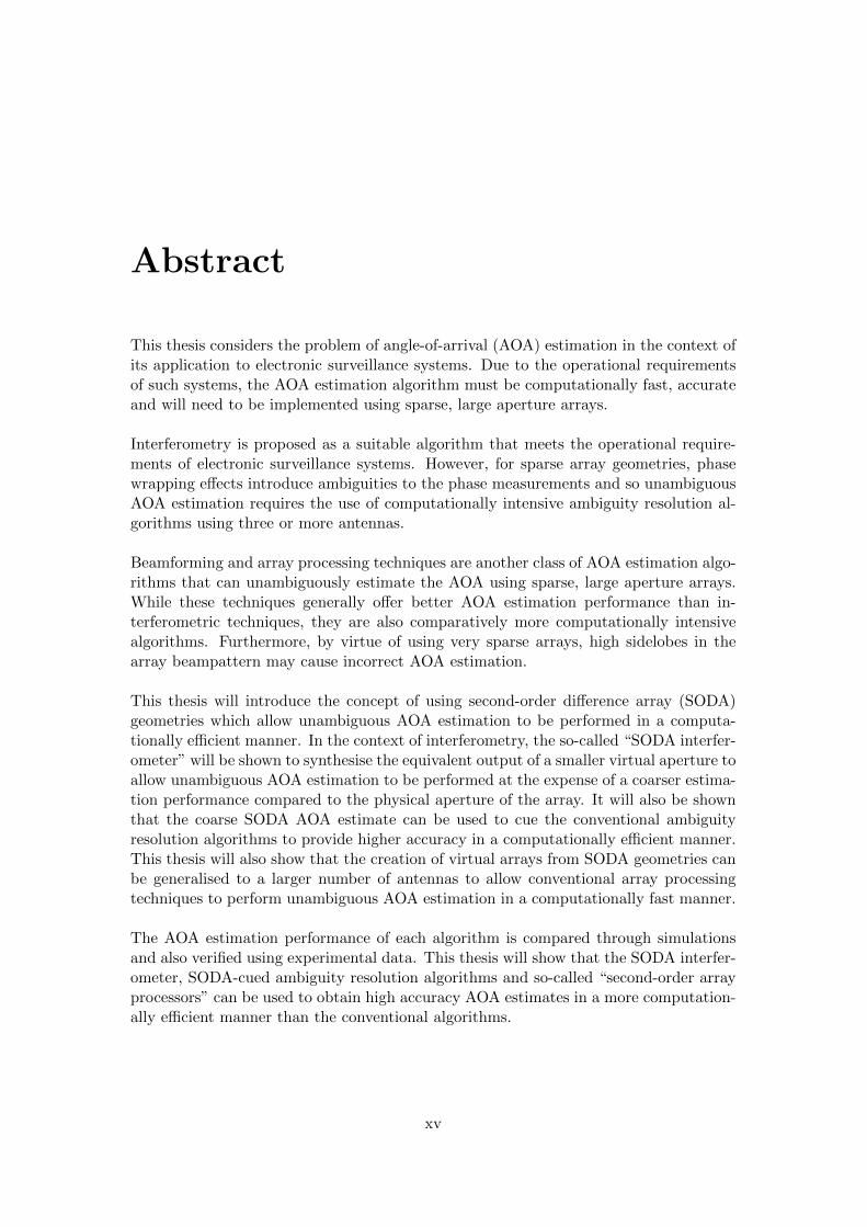
This thesis considers the problem of angle-of-arrival (AOA) estimation in the context ofits application to electronic surveillance systems. Due to the operational requirementsof such systems, the AOA estimation algorithm must be computationally fast, accurateand will need to be implemented using sparse, large aperture arrays.

Interferometry is proposed as a suitable algorithm that meets the operational require-ments of electronic surveillance systems. However, for sparse array geometries, phasewrapping effects introduce ambiguities to the phase measurements and so unambiguousAOA estimation requires the use of computationally intensive ambiguity resolution al-gorithms using three or more antennas.

Beamforming and array processing techniques are another class of AOA estimation algo-rithms that can unambiguously estimate the AOA using sparse, large aperture arrays.While these techniques generally offer better AOA estimation performance than in-terferometric techniques, they are also comparatively more computationally intensivealgorithms. Furthermore, by virtue of using very sparse arrays, high sidelobes in thearray beampattern may cause incorrect AOA estimation.

This thesis will introduce the concept of using second-order difference array (SODA)geometries which allow unambiguous AOA estimation to be performed in a computa-tionally efficient manner. In the context of interferometry, the so-called “SODA interfer-ometer” will be shown to synthesise the equivalent output of a smaller virtual aperture toallow unambiguous AOA estimation to be performed at the expense of a coarser estima-tion performance compared to the physical aperture of the array. It will also be shownthat the coarse SODA AOA estimate can be used to cue the conventional ambiguityresolution algorithms to provide higher accuracy in a computationally efficient manner.This thesis will also show that the creation of virtual arrays from SODA geometries canbe generalised to a larger number of antennas to allow conventional array processingtechniques to perform unambiguous AOA estimation in a computationally fast manner.

The AOA estimation performance of each algorithm is compared through simulationsand also verified using experimental data. This thesis will show that the SODA interfer-ometer, SODA-cued ambiguity resolution algorithms and so-called “second-order arrayprocessors” can be used to obtain high accuracy AOA estimates in a more computation-ally efficient manner than the conventional algorithms.

xv

xvi

Declaration

I certify that this work contains no material which has been accepted for the award ofany other degree or diploma in my name, in any university or other tertiary institutionand, to the best of my knowledge and belief, contains no material previously publishedor written by another person, except where due reference has been made in the text. Inaddition, I certify that no part of this work will, in the future, be used in a submissionin my name, for any other degree or diploma in any university or other tertiary institu-tion without the prior approval of the University of Adelaide and where applicable, anypartner institution responsible for the joint-award of this degree.

I give consent to this copy of my thesis, when deposited in the University Library, beingmade available for loan and photocopying, subject to the provisions of the CopyrightAct 1968.

I also give permission for the digital version of my thesis to be made available on the web,via the University’s digital research repository, the Library Search and also through websearch engines, unless permission has been granted by the University to restrict accessfor a period of time.

........................................................................Peter Quoc Cuong Ly

3 December 2013

xvii

xviii

Acknowledgements

I would like to thank my university supervisor, Professor Doug Gray, for encouragingme to enter the field of signal processing. It was under your mentorship during myfinal years as a undergraduate student that sparked my interest in a career in signalprocessing research. Thank you for all of your time, effort and patience over the last tenyears. Without your support and encouragement, the completion of this thesis wouldnot have been possible.

I would also like to thank my DSTO supervisor, Dr Stephen Elton, for bringing thisPhD to fruition. This thesis would not have been possible without your tireless effortsin negotiating the agreement between the university and DSTO. Your friendship andunwavering support both academically and personally during this candidacy has beenan invaluable source of encouragement.

I would also like to thank my co-supervisor, Professor Bevan Bates, for helping menavigate through the necessary administration at the university and DSTO and alsofor allowing me to join in on a number of experiments to collect experimental data tosupport this PhD research.

I am grateful for the support of my DSTO superiors, Dr Len Sciacca, Dr Jackie Craig,Dr Warren Marwood, Dr Peter Gerhardy and Brian Reid, for providing me with the op-portunity to undertake this PhD research as part of my DSTO working arrangements. Iam also grateful for the support from my DSTO colleagues, including but not limited toSimon Herfurth, John Quin, Phil Wandel, Jarrad Shiosaki, Andrew Evans and SongsriSirianunpiboon for their assistance with the hardware development and experimentaltrials.

I would like to express my gratitude to my family for their unconditional love and sup-port. I would like to thank my parents for instilling in me the appreciation of academicexcellence and the value of persistence. I would also like to thank my sister for ground-ing me in reality.

Finally, I thank my wife, Joy, for being my rock during the last seven years. Not only doyou deserve credit for helping me academically, but your unwavering support, patienceand faith in me helped me get through some of my darkest times. You are my light.

xix

xx

Publications

Some parts of this thesis have been published for presentation at conferences. The fol-lowing list is the bibliographic information pertaining to these preliminary presentations.

• Ly, P. Q. C., Elton, S. D., Li, J. & Gray, D. A., “Computationally Fast AOAEstimation Using Sparse Large Aperture Arrays for Electronic Surveillance,” inProceedings of the IEEE International Conference on Radar (RADAR 2013), 2013.Accepted.

• Ly, P. Q. C., Elton, S. D., Gray, D. A., & Li, J., “Unambiguous AOA EstimationUsing SODA Interferometry for Electronic Surveillance,” in Proceedings of theIEEE Sensor Array and Multichannel Signal Processing Workshop (SAM 2012),pp. 277–280, 2012.

• Ly, P. Q. C., Gray, D. A., Elton, S. D., & Bates, B. D., “A Digital InterferometricTestbed for ES/ELINT Research,” in Proceedings of the Seventh Direction Findingand Geolocation Symposium, 2008.

xxi

xxii

xxiii

Acronyms

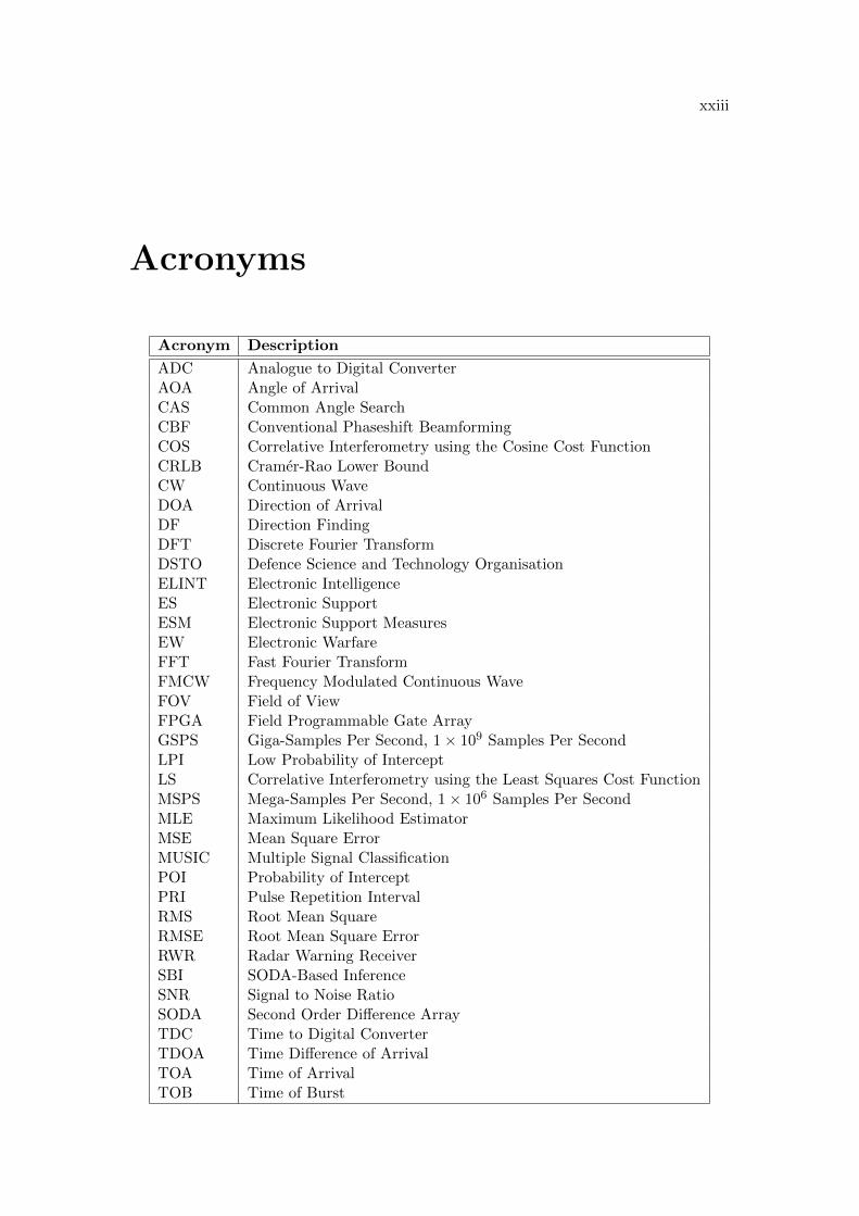
Acronym Description

ADC Analogue to Digital ConverterAOA Angle of ArrivalCAS Common Angle SearchCBF Conventional Phaseshift BeamformingCOS Correlative Interferometry using the Cosine Cost FunctionCRLB Cramer-Rao Lower BoundCW Continuous WaveDOA Direction of ArrivalDF Direction FindingDFT Discrete Fourier TransformDSTO Defence Science and Technology OrganisationELINT Electronic IntelligenceES Electronic SupportESM Electronic Support MeasuresEW Electronic WarfareFFT Fast Fourier TransformFMCW Frequency Modulated Continuous WaveFOV Field of ViewFPGA Field Programmable Gate ArrayGSPS Giga-Samples Per Second, 1× 109 Samples Per SecondLPI Low Probability of InterceptLS Correlative Interferometry using the Least Squares Cost FunctionMSPS Mega-Samples Per Second, 1× 106 Samples Per SecondMLE Maximum Likelihood EstimatorMSE Mean Square ErrorMUSIC Multiple Signal ClassificationPOI Probability of InterceptPRI Pulse Repetition IntervalRMS Root Mean SquareRMSE Root Mean Square ErrorRWR Radar Warning ReceiverSBI SODA-Based InferenceSNR Signal to Noise RatioSODA Second Order Difference ArrayTDC Time to Digital ConverterTDOA Time Difference of ArrivalTOA Time of ArrivalTOB Time of Burst

xxiv

Notation

Symbols

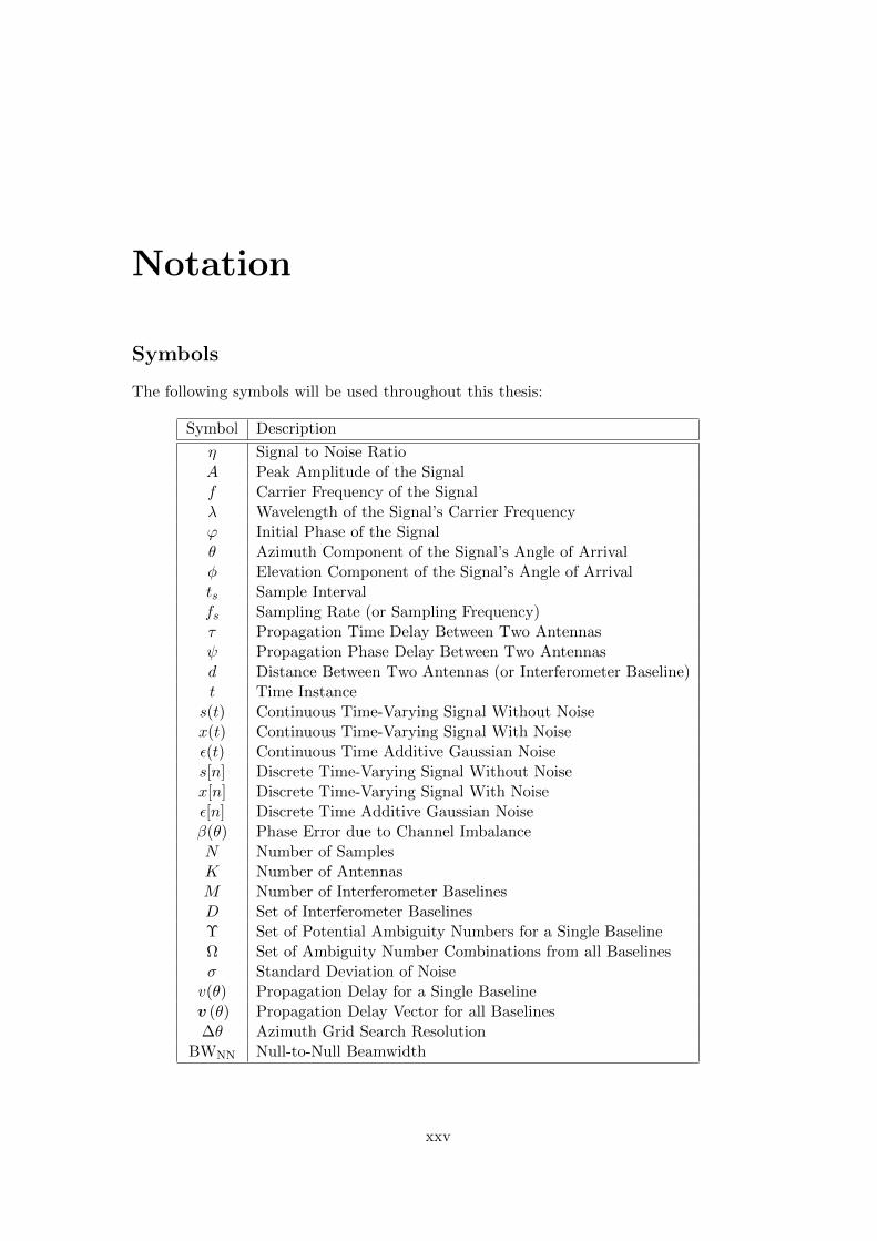
The following symbols will be used throughout this thesis:

Symbol Description

η Signal to Noise RatioA Peak Amplitude of the Signalf Carrier Frequency of the Signalλ Wavelength of the Signal’s Carrier Frequencyϕ Initial Phase of the Signalθ Azimuth Component of the Signal’s Angle of Arrivalφ Elevation Component of the Signal’s Angle of Arrivalts Sample Intervalfs Sampling Rate (or Sampling Frequency)τ Propagation Time Delay Between Two Antennasψ Propagation Phase Delay Between Two Antennasd Distance Between Two Antennas (or Interferometer Baseline)t Time Instances(t) Continuous Time-Varying Signal Without Noisex(t) Continuous Time-Varying Signal With Noiseε(t) Continuous Time Additive Gaussian Noises[n] Discrete Time-Varying Signal Without Noisex[n] Discrete Time-Varying Signal With Noiseε[n] Discrete Time Additive Gaussian Noiseβ(θ) Phase Error due to Channel ImbalanceN Number of SamplesK Number of AntennasM Number of Interferometer BaselinesD Set of Interferometer BaselinesΥ Set of Potential Ambiguity Numbers for a Single BaselineΩ Set of Ambiguity Number Combinations from all Baselinesσ Standard Deviation of Noisev(θ) Propagation Delay for a Single Baselinev (θ) Propagation Delay Vector for all Baselines∆θ Azimuth Grid Search Resolution

BWNN Null-to-Null Beamwidth

xxv

xxvi

Scripts and Accents

Scripts and accents will be used to confer additional meaning to the above symbols.

• A single letter subscript specifies that the associated parameter belongs to a spe-cific hardware channel. For example, Ak and fk refers to the peak amplitude andcarrier frequency of the k-th receiver channel. A single letter subscript can alsospecify that the parameter belongs to a particular interferometric baseline. Forexample, ψm and dm refers to the phase delay and baseline of the m-th interfer-ometer baseline. When only a single letter subscript is used, it is generally impliedthat the specified parameter refers to an arbitrary interferometer baseline.

• A double letter subscript specifies the parameter of a particular channel withrespect to another channel. For example, ψkl and dkl refers to the phase delay andinterferometer baseline of the k-th antenna relative to the l-th antenna. When adouble letter subscript is used, it is generally implied that the specified parameterrefers to a specific interferometer baseline.

• The subscript s specifies a steered parameter that is under the control of the radarintercept receiver. For example, θs refers to the steered AOA of a grid searchalgorithm for AOA estimation.

• The superscript u specifies an uncalibrated parameter that is subject to channelimbalances.

• The superscript c specifies a calibrated parameter free of channel imbalances.

• The tilde accent˜specifies a measured parameter. In particular, when specifyingthe phase delay measurement, ψ refers to the unwrapped, unambiguous phase de-lay, however, ψ refers to the measured, ambiguous phase delay that is constrainedto the interval [−π, π].

• The hat accentˆspecifies an estimated parameter.

• Plain typeface symbols, e.g. v(θ), are used to denote scalar variables.

• Bold typeface symbols in lower case characters, e.g. v (θ), are used to denotevector variables.

• Bold typeface symbols in upper case characters, e.g. R , are used to denote matrixvariables.

Mathematical Operators

Operator Description

round [a] Rounds the scalar a to the nearest integer.dae Rounds the scalar a upwards to the next integer.bac Rounds the scalar a downwards to the next integer. Cartesian product.

a T or A T Transpose of the vector, a , or matrix, A .

aH or AH Hermitian (complex conjugate) transpose of the vector, a , or matrix, A .

xxvii

Units

All parameters are assumed to adhere to the International System of Units (or SI units).

The units of phase-related values, such as the phase delay and angle-of-arrival, areassumed to be expressed in radians for all mathematical expressions. However, forreadability, the phase-related values will often be expressed in degrees in the text andfigures.

Documents

Fast and Unambiguous Direction Finding for Digital Radar ...€¦ · Fast and Unambiguous Direction Finding for Digital Radar Intercept Receivers Peter Quoc Cuong Ly A Thesis Submitted