Fall 2002. 10.34. Numerical Methods Applied to Chemical Engineering

Homework # 2. Nonlinear algebraic equations

Solution set Problem 1. Tank-draining problem Question 1.A. Plot the volumetric flow rate out of the tank as a function of h. First we pick the bottom of pipe as a reference height (any height can be chosen but this is most convenient) Now using that reference height, we specify the total pressure on the surface of the water and at the exit of the pipe Pttop = Patm +½ �V2

top + �g(h+L) Ptexit = Patm +½ �V2 Where Vtop= V(Apipe/Atop)=V((¼�D2)/(¼�D2

top))=V(D/Dtop)2=(0.05[m]/2.5[m])2=4*10-

4V We use Bernoulli’s equation to relate Pttop and Ptexit remembering to account for losses in total pressure. (Bernoulli’s equation can be thought of as a mechanical energy balance. The word mechanical is used to distinguish it from the thermal energy balance used for compressible flows.) Ptexit = Pttop – losses Patm +½ �V2 = Patm + ½ �V2

top + �g(h+L) – losses ½ �V2 = ½ �V2

top + �g(h+L) - losses But what are the losses? lossentrance = ¼�V2 losspipe = fD(L/D)(½ �V2) ½ �V2 = ½ �V2

top + �g(h+L) -¼�V2 - fD(L/D)(½ �V2) Since there are 2 equations (laminar and turbulent flow) for the Darcy friction factor, fD, we need to check if the laminar flow formulation, fD = 64/Re, will be used. A “best case” scenario (if it’s not used then, it never will be) is when the water height, h, in the tank is infinitesimal. (This implies that the entrance loss and that Vtop=4*10-4V still apply). We assume that the flow is laminar and that �=�/�=10-6 [m2/s] (kinematic viscosity for water at 20o C). The pipe diameter D=0.05 [m] so the Reynolds number is Re= �VD/� = VD/� =5*104 V. The laminar Darcy friction factor is then fD = 64/Re = 0.00128/V (where V is in [m/s]). The pipe length, L=2 [m]. Acceleration due to gravity is g=9.8065 [m/s2]

½ �V2 = ½ �(4*10-4 V)2 + �gL -¼�V2 - fD(L/D)(½ �V2) 1.49999984 V2 = 2gL - fD(L/D)V2 1.49999984 V2 = 39.226 –0.0512 V V=4.1583 [m/s] For laminar flow, Re < 2100 or V < 2100/(5*104 ) = 0.042 [m/s]. Since the best case V is much greater than this, the flow will always turbulent.

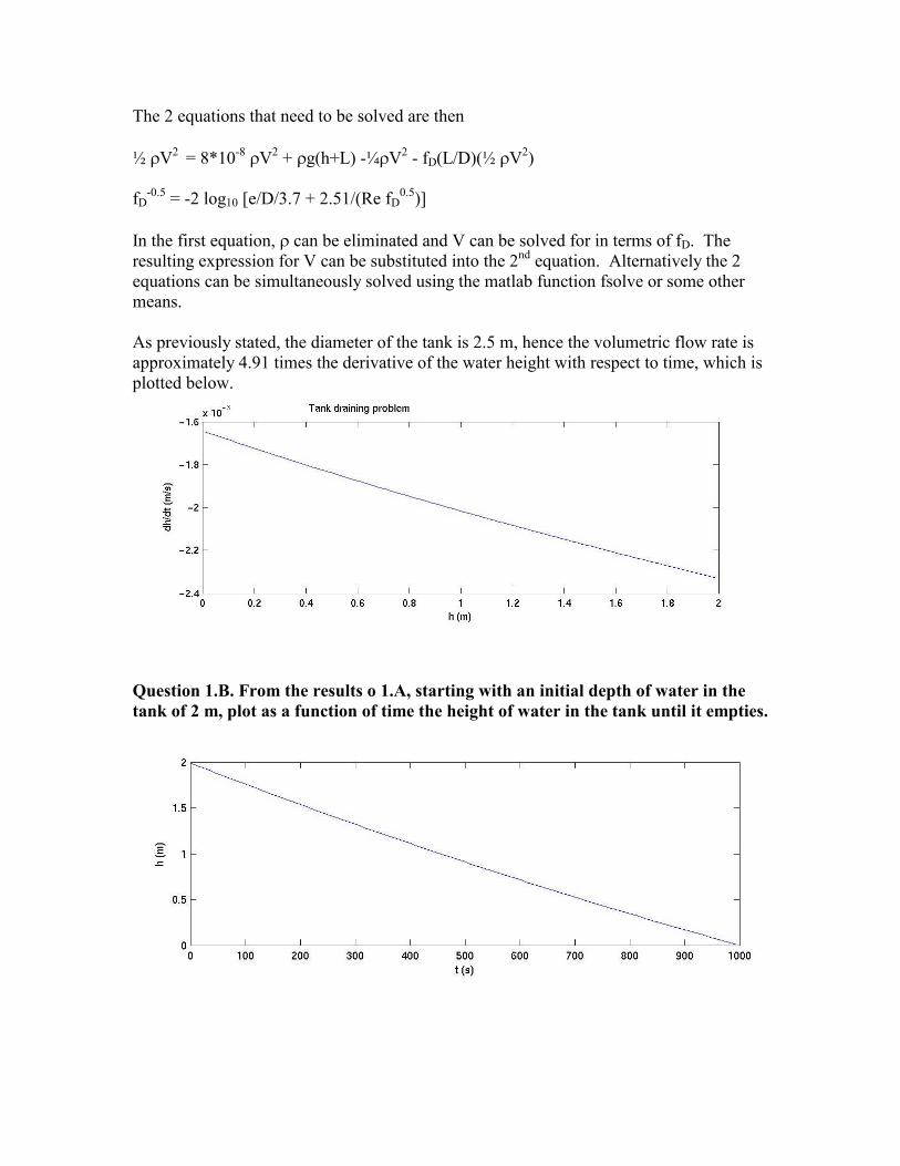
The 2 equations that need to be solved are then ½ �V2 = 8*10-8 �V2 + �g(h+L) -¼�V2 - fD(L/D)(½ �V2) fD

-0.5 = -2 log10 [e/D/3.7 + 2.51/(Re fD0.5)]

In the first equation, � can be eliminated and V can be solved for in terms of fD. The resulting expression for V can be substituted into the 2nd equation. Alternatively the 2 equations can be simultaneously solved using the matlab function fsolve or some other means. As previously stated, the diameter of the tank is 2.5 m, hence the volumetric flow rate is approximately 4.91 times the derivative of the water height with respect to time, which is plotted below.

Question 1.B. From the results o 1.A, starting with an initial depth of water in the tank of 2 m, plot as a function of time the height of water in the tank until it empties.

The following matlab code was written by Professor Beers as a solution to this problem. % plot_dh_dt_tank_drain_v2.m % % This MATLAB m-file makes a plot of dh/dt vs. h % for the tank draining problem, and plots the % tank height as a function of time. % K. Beers. MIT ChE. 9/19/02 function iflag_main = plot_dh_dt_tank_drain_v2(); iflag_main = 0; % set problem parameters Param.Dt = 2.5; % tank diameter in m Param.Dp = 5e-2; % pipe diameter in m Param.L = 2; % drain pipe length in m Param.density = 1000; % water density in Kg/m^3 Param.viscosity = 1e-3; % water viscosity in Pa*s Param.e = 4.5e-5; % effective surface roughness of pipe (m) Param.e_D = Param.e/Param.Dp; % relative surface roughness Param.g = 9.8; % gravity acceleration (m/s^2) Param.K_L = 0.5; % entrance loss coefficient % Set maximum tank height (m) h_max = 2; % set minimum tank height (m) h_min = 0.01; % set interval in height values (m) dh = 0.02; % Set grid of tank height values h_grid = [h_min : dh : h_max]; num_h = length(h_grid); % Allocate vector to store output values dh_dt_grid = zeros(size(h_grid)); Q_grid = zeros(size(h_grid)); V_grid = zeros(size(h_grid)); Re_grid = zeros(size(h_grid)); fd_grid = zeros(size(h_grid)); % Use initial guess of infinite Re limit % for commercial steel pipe.

fd_guess = 0.02; % Call solver to compute results for each h value. verbose = 0; for k = num_h : -1 : 1 [dh_dt_grid(k),Q_grid(k),... V_grid(k),Re_grid(k),fd_grid(k)] = ... tank_drain(h_grid(k),fd_guess,Param,verbose); % store friction factor as guess for next % iteration fd_guess = fd_grid(k); end % Now, estimate times at which tank reaches each height time = zeros(size(h_grid)); for k = (num_h-1) : -1 : 1 dt = (h_grid(k)-h_grid(k+1))/dh_dt_grid(k+1); time(k) = time(k+1) + dt; end % Make plots of results figure; % tank height rate of change subplot(2,1,1); plot(h_grid,dh_dt_grid); xlabel('h (m)'); ylabel('dh/dt (m/s)'); % tank height vs. time subplot(2,1,2); plot(time,h_grid); xlabel('t (s)'); ylabel('h (m)'); gtext('Tank draining problem'); % new figure for other results figure; % Velocity in drain pipe subplot(2,2,1); plot(h_grid,V_grid); xlabel('h (m)'); ylabel('V (m/s)'); % volumetric flow rate subplot(2,2,2); plot(h_grid,Q_grid); xlabel('h (m)'); ylabel('Q (m^3/s)');

% Reynolds' number in drain pipe subplot(2,2,3); semilogy(h_grid,Re_grid); xlabel('h (m)'); ylabel('Re'); % friction factor subplot(2,2,4); plot(h_grid,fd_grid); xlabel('h (m)'); ylabel('f_D'); gtext('Tank draining problem'); iflag_main = 1; return; % ============================================== % tank_drain.m % % This MATLAB program calculates the velocity % through the exit pipe for a tank-draining % problem at a specified value of the height % of water in the tank. % % K. Beers % MIT ChE. 9/18/02 % v 2. 9/19/02 function [dh_dt,Q,V,Re,fd,iflag_main] = ... tank_drain(h,fd_guess,Param,verbose); iflag_main = 0; if(~exist('verbose')) verbose = 0; end Param.h = h; % tank height in m - INPUT VALUE % For this initial guess of the friction factor, we calculate % the corresponding value of the velocity from the macroscopic % energy balances. V_guess = tank_drain_calc_V(fd_guess,Param);

Re_guess = Param.density*V_guess*Param.Dp/Param.viscosity; if(verbose) disp(['Guess fd = ', num2str(fd_guess)]); disp(['Guess velocity = ', num2str(V_guess)]); disp(['Guess Reynolds'' number = ', num2str(Re_guess)]); end % Now, with this initial guess of the friction factor, % we use the MATLAB command fzero to solve the resulting % nonlinear algebraic equation for fd. options = optimset('Display','off'); if(verbose) options = optimset('Display','iter'); end [fd,fval,exitflag,output] = fzero(@tank_drain_calc_f, ... fd_guess,options,Param); % From the final value of the friction factor, we calculate % the velocity through the pipe. V = tank_drain_calc_V(fd,Param); % the Reynolds' number Re = Param.density*V*Param.Dp/Param.viscosity; % the volumetric flow rate through the drain pipe (m^3/2) Q = pi/4*Param.Dp^2*V; % the rate of change of the height of the tank (m/s) dh_dt = -Q/(pi/4*Param.Dt^2); if(verbose) disp(['Darcy friction factor = ', num2str(fd)]); disp(['Drain pipe velocity (m/s) = ', num2str(V)]); disp(['Pipe Reynolds'' number = ', num2str(Re)]); disp(['Volumetric flow rate (m^3/s) = ', num2str(Q)]); disp(['Rate of change of height (m/s) = ', num2str(dh_dt)]); end iflag_main = 1; return; % =========================================================== % This MATLAB function calculates the velocity through the % drain pipe as a function of the Darcy friction factor.

% K. Beers. MIT ChE. 9/18/02 function V = tank_drain_calc_V(fd,Param); var1 = 1 - (Param.Dp/Param.Dt)^4 + Param.K_L + ... fd*Param.L/Param.Dp; V = sqrt(2*Param.g*(Param.h+Param.L)/var1); return; % ========================================================== % This MATLAB function calculates the function values % that goes to zero when the value of the Darcy % friction factor satisfies the problem. % K. Beers. MIT ChE. 9/18/02 % v. 2. 9/20/02 function fval = tank_drain_calc_f(x,Param); fd = x; % For this value of the friction factor, calculate % the corresponding velocity from the balance % equations. V = tank_drain_calc_V(fd,Param); % From this velocity, calculate the Reynolds' number % in the pipe. Re = Param.density*V*Param.Dp/Param.viscosity; % If Re < 2100, laminar flow if(Re < 2100) fval = fd - 64/Re; % else for turbulent flow, use Colebrook equation else var1 = Param.e_D/3.7 + 2.51/Re/sqrt(fd); fval = 1/sqrt(fd) + 2*log10(var1); end return; Problem 2. Modeling steady-state behavior of a Nylon reaction system.

Question 2.A.1, using this statistical model, plot the chain length distributions at conversions of 25%, 50%, 75%, 90%, 92.5%, 95%, 97.5%, 99%, 99.5%, 99.75%, and 99% “this statistical model” refers to equation 32 from the assignment sheet (reprinted here).

The following matlab code generated the above chain length distributions plot. close all; clear %conversion p=[.25 .50 .75 .90 .925 .95 .975 .99 .995 .9975 .999]'; %%%%%%%%%%%%%%%%%%%%%%%%%%%%%%%%%%%% %Question 2.A.1 %%%%%%%%%%%%%%%%%%%%%%%%%%%%%%%%%%%% for i=1:length(p) if(any(i==[1 4 8])) %3 plots on 1st page 4 on next 2 fig=figure; position=get(fig,'Position'); %on screen window size position(2)=position(2)-2/3*position(4); %lower window bottom position(4)=position(4)*5/3; %increase window height set(fig,'PaperPosition',[0.25 0.5 8 10],'Position',position) end subplot(4,1,mod(i,4)+1); xn=1/(1-p(i))*[1 1]; xw=(1+p(i))/(1-p(i))*[1 1]; xmax=2*max(xn(1),xw(1)); x=floor([0:xmax/64:xmax])'; P=p(i).^x.*(1-p(i)).^2; y=[min(P) max(P)]; plot(x,P,'-b',xn,y,'-r',xw,y,'-r'); ytext=y*[.20; .8]; text(xn(1),ytext,'x_n'); %label xn line text(xw(1),ytext,'x_w'); %label xw line text(5/8*xmax,ytext,sprintf('conversion p=%g',p(i))); %list conversion if(any(i==[1 4 8])) title('Question 2.A.1'); end xlabel('chain length x'); ylabel('[P_x]/[P_1]_0'); grid on; axis tight; %automatically print to jpeg files if(any(i==[3 7 11])) eval(sprintf('print -djpeg p2A1_%g.jpg',fig)); end end

Question 2.A.2, use your results from 2.A.1 to plot, as functions of the conversion, the number and weight average chain lengths and the polydispersity. Make sure that you consider high-enough chain lengths in your summation that the weight-average chain length and polydispersity converge closely to their true values. The simplified equations used to calculate xn, xw, and Z are derived in a straight-forward manner:

These equations are plotted below with infinity approximated as 10000.

The matlab code used to generate these plots follows: p=[.25 .50 .75 .90 .925 .95 .975 .99 .995 .9975 .999]'; %conversion m=1:10000; xn=zeros(size(p)); xw=xn; for i=1:length(p) xn(i)=sum(m.*p(i).^(m-1))/sum(p(i).^(m-1)); xw(i)=sum(m.^2.*p(i).^(m-1))/sum(m.*p(i).^(m-1)); end z=xw./xn; figure; subplot(3,1,1); plot(p,xn); ylabel('x_n'); axis tight; grid on; title('Question 2.A.2') subplot(3,1,2); plot(p,xw); ylabel('x_w'); axis tight; grid on; subplot(3,1,3); plot(p,z); ylabel('Z'); axis tight; grid on; xlabel('conversion: p') Question 2.A.3. From your results in 2.A.2, propose the corresponding formulas for xw and Z. xn, xw, and Z are expressed without an infinite series as:

This pattern of Z =1+p is readily observable from the previous plots. As “proof”, plots identical to those found in part 2.A.2 were generated from these functions of conversion.

The code that generated these plots follows. p=[.25 .50 .75 .90 .925 .95 .975 .99 .995 .9975 .999]'; %conversion Xn=1./(1-p); Xw=2*Xn-1; Z=p+1; figure; subplot(3,1,1); plot(p,Xn); ylabel('x_n=1/(1-p)'); axis tight; grid on; title('Question 2.A.3') subplot(3,1,2); plot(p,Xw); ylabel('x_w=(1+p)/(1-p)'); axis tight; grid on; subplot(3,1,3); plot(p,Z); ylabel('Z=1+p'); axis tight; grid on; xlabel('conversion: p')

Part 2.B. Modeling the continuous polymerization process. Question 2.B.1 Write a MATLAB program that computes p, xn, xw, and Z for each reactor in the 3 CSTR process shown in the diagram above. (diagram not included in solution set) While coding style varies the equations central to solving this program are not. Their derivation is as follows. The rate reactions for �0, �2, and W are:

k(fc) needs to be replaced in all three rate equations. A, B, and L also need to be replaced in the rate equation for water production.

These rates are then substituted into “mass balance” equations. Derivatives with respect to time are set to zero because a steady state reaction is being modeled.

The resulting equations (the ones to be used in the matlab program) are:

The matlab code written by Professor Beers as a solution for this problem follows: % Nylon_polycond.m % % This MATLAB program calculates the conversions and % averaged chain lengths of Nylon polymer produced % in a 3 CSTR process. Moment equations with the % Schultz-Flory closure approximation for the 3rd % moment are used. Equal balance between diamine % and diacid monomers is assumed. % % K. Beers. MIT ChE. 9/16/2002 function [xn,xw,Z,p,iflag_main] = ... Nylon_polycond(); iflag_main = 0; % First, set the simulation parameters. lambda_1 = 1; % first moment of CLD % the monomer feed CLD moments % and water concentation lambda_0_feed = 1; lambda_2_feed = 1; W_feed = 0; % the equilibrium constant Keq = 100; % the reference Daemkohler number % of the first reactor. The other % reactors are set to have the same

% volume, so the Damkohler number % of a CSTR is equal to % Da_ref*lambda_0_in. Da_ref = 50; % the user is now prompted to input the % common (km*A/V)*tres - the product of the mass % transfer coefficient with the area/volume % and the residence time of the reactor. % If a column vector is input, the calculation % is repeated for each value of the kmApV_min = input('Input min. (k_m A / V)*t_res : '); kmApV_max = input('Input max. (k_m A / V)*t_res : '); num_kmApV = input('Input number of kmApV values : '); km_A_per_V_tres = logspace(log10(kmApV_min), ... log10(kmApV_max), num_kmApV); % if 1, plots are to be made iplot = 1; % For each value of the mass transfer coefficient, % we repeat the calculation of the polymer properties % in each reactor. First, we allocate space for % the results. % number-averaged chain lengths in each CSTR xn = zeros(num_kmApV,3); % weight-averaged chain lengths in each CSTR xw = zeros(num_kmApV,3); % polydispersities in each CSTR Z = zeros(num_kmApV,3); % conversions in each CSTR p = zeros(num_kmApV,3); % iterate over each mass transfer value for i_kmApV = 1:num_kmApV kmApV_tres = km_A_per_V_tres(i_kmApV); % use sequential approach to compute % polymer properties in each reactor lambda_0_in = lambda_0_feed; lambda_2_in = lambda_2_feed; W_in = W_feed; for i_CSTR = 1:3 [lambda_0,lambda_2,W,iflag] = ... polycond_CSTR_SS(lambda_0_in, ...

lambda_2_in, W_in, Da_ref, ... kmApV_tres, Keq, lambda_1); if(iflag >= 1) % success % record results xn(i_kmApV,i_CSTR) = lambda_1/lambda_0; xw(i_kmApV,i_CSTR) = lambda_2/lambda_1; Z(i_kmApV,i_CSTR) = lambda_2*lambda_0/lambda_1^2; p(i_kmApV,i_CSTR) = 1 - lambda_0/lambda_1; % use as input to next CSTR lambda_0_in = lambda_0; lambda_2_in = lambda_2; W_in = W; else error(['polycond_CSTR_SS: iflag = ', ... int2str(iflag)]); end end end

% graph results if(iplot ~= 0) figure; % xn vs. kmApV subplot(2,2,1); semilogx(km_A_per_V_tres,xn(:,1)); hold on; semilogx(km_A_per_V_tres,xn(:,2),'-.'); semilogx(km_A_per_V_tres,xn(:,3),':'); axis([kmApV_min, kmApV_max, 1, 1.1*max(max(xn))]); xlabel('(k_m A / V)\theta'); ylabel('x_n'); legend('1', '2', '3',2); % xw vs. kmApV subplot(2,2,2); semilogx(km_A_per_V_tres,xw(:,1)); hold on; semilogx(km_A_per_V_tres,xw(:,2),'-.'); semilogx(km_A_per_V_tres,xw(:,3),':'); axis([kmApV_min, kmApV_max, 1, 1.1*max(max(xw))]); xlabel('(k_m A / V)\theta'); ylabel('x_w'); % Z vs. kmApV subplot(2,2,3); semilogx(km_A_per_V_tres,Z(:,1)); hold on; semilogx(km_A_per_V_tres,Z(:,2),'-.'); semilogx(km_A_per_V_tres,Z(:,3),':'); axis([kmApV_min, kmApV_max, 1, 1.1*max(max(Z))]); xlabel('(k_m A / V)\theta'); ylabel('Z'); % p vs. kmApV subplot(2,2,4); semilogx(km_A_per_V_tres,p(:,1)); hold on; semilogx(km_A_per_V_tres,p(:,2),'-.'); semilogx(km_A_per_V_tres,p(:,3),':'); axis([kmApV_min, kmApV_max, 0.9*min(min(p)), 1]); xlabel('(k_m A / V)\theta'); ylabel('p'); gtext('3 CSTR Nylon polycondensation process'); end iflag_main = 1; return;

% ========================================================= % This MATLAB routine computes the values of each moment % in a CSTR at steady state for a simple condensation system. % K. Beers. MIT ChE. 9/16/02 function [lambda_0,lambda_2,W,iflag] = ... polycond_CSTR_SS(lambda_0_in, ... lambda_2_in, W_in, Da_ref, ... kmApV_tres, Keq, lambda_1); iflag = 0; % First, make initial guesses for the % moments based on the inlet concentrations lambda_0_guess = lambda_0_in; lambda_2_guess = lambda_2_in; W_guess = W_in; % stack guesses into column vector x_guess = [lambda_0_guess; lambda_2_guess; W_guess]; % set Daemkohler number based on input concentration. % This has effect that all CSTR's are of the same % volume. Da = Da_ref * lambda_0_in; % Since this guess should be exact when the residence % time goes to zero, we use homotopy. num_homotopy = 10; for i_homotopy = 1:num_homotopy kmApV_tres_work = ... i_homotopy/num_homotopy * ... kmApV_tres; Da_work = ... i_homotopy/num_homotopy * Da; % call MATLAB fsolve() to solve system of equations options = optimset('TolFun',1e-8,'LargeScale','off', ... 'Display','off'); [x,fval,exitflag] = fsolve(@fun_polycond_CSTR_SS, ... x_guess,options,lambda_0_in, lambda_2_in, W_in, ... Da_work, kmApV_tres_work, Keq, lambda_1); x_guess = x; end

% assign output lambda_0 = x(1); lambda_2 = x(2); W = x(3); iflag = exitflag; return; % ========================================================= % This MATLAB routine computes the function values for the % governing equations of a polycondensation CSTR at steady % state. % K. Beers. MIT ChE. 9/16/02 function [f,iflag] = ... fun_polycond_CSTR_SS(x, ... lambda_0_in, lambda_2_in, ... W_in, Da, ... kmApV_tres, Keq, lambda_1); iflag = 0; % unstack unknowns into real-life names lambda_0 = x(1); lambda_2 = x(2); W = x(3); % allocate vector for function values f = zeros(3,1); % compute third moment from closure approximation lambda_3 = lambda_2*(2*lambda_2*lambda_0 - lambda_1^2) ... / (lambda_1*lambda_0); % balance for zeroth moment f(1) = lambda_0_in - lambda_0 + Da/lambda_0_in * ... (-lambda_0^2 + W/Keq*(lambda_1-lambda_0)); % balance for zecond moment f(2) = lambda_2_in - lambda_2 + Da/lambda_0_in * ... (2*lambda_1^2 + W/Keq/3*(lambda_1 - lambda_3)); % balance for water condensate

f(3) = W_in - W - kmApV_tres*W + ... Da/lambda_0_in * ... (lambda_0^2 - W/Keq*(lambda_1-lambda_0)); return;

Question 2.B.2. Using a Damkohler number of 50 for the first CSTR, plot as functions of (km A / V)� the number-averaged and weight-averaged chain lengths, the polydispersities, and the conversions in the product streams from each reactor.

Explain why one observes limiting values of the chain lengths as (km A / V)�➜ 0 and (km A / V)�➜ �. (km A / V)� is a measure of the purge gas stream’s ability to take on and remove water. The lower limit levels out because essentially no water is being removed. The upper limit is set but the reactor residence time. As the Damkohler number approaches infinity, the reaction rate approaches its equilibrium value. The equilibrium constant of the reaction is defined to be Keq=[L]eq[W]eq/([A]eq[B]eq). Using equation 37 (and noting that water is produced in proportion to the linkages) we get: Keq=(�1-�0)2/�0

2. Hence xn=�1/�0=1+Keq

½, xw is similarly set by Keq. Why is the polydispersity greater for large mass transfer rates than would be expected for a batch polymerization, where the chain length distribution follows the Flory statistical model? As (km A / V)�➜ � the reverse reaction is increasingly penalized. We get high polydispersity, Z, because of the residence time distribution. Some chains take longer

than others to pass through the reactor. These chains have a chance to grow longer than those that pass through immediately. This results in a Z > 2. Why does the polydispersity decrease as the mass transfer rate decreases? As (km A / V)�➜ 0 less or even no water is removed. Longer chains have more linkages so they are a “bigger target” for reverse reactions, that is they are more likely to be broken up. This limits the polydispersity.