Embed Size (px)
Citation preview
Fain et al. Particulate Dynamics in a River Estuary
Seasonal and Tidal-Monthly Patterns of Particulate Matter Dynamics in a River Estuary
Annika M.V. Fain1
School of Oceanography
University of Washington
Box 357940
Seattle, WA 98195
David A. Jay
Doug J. Wilson
Phil M. Orton
Antonio M. Baptista
Environmental Science and Engineering
Oregon Graduate Institute
20000 NW Walker Rd.
Beaverton, OR 97006
1-Corresponding author; tele:206/543-6454; fax:206/543-0275; e-mail
Fain et al.2
Abstract
We have investigated seasonal and tidal-monthly suspended particulate matter (SPM) dynamics
in the Columbia River Estuary from May to December 1997 using acoustic backscatter (ABS) and
velocity data from four long-term Acoustic Doppler Profiler (ADP) moorings in or near the estuarine
turbidity maximum (ETM). The ABS was calibrated and converted to total SPM using vessel data
obtained during three seasonal cruises, employing optical backscatter (OBS) as an intermediary. Four
characteristic settling velocity (Ws) classes were defined from Owen Tube samples collected during the
cruises. An inverse analysis, in the form of a non-negative least squares minimization, was used to
determine the contribution of the four Ws-classes to each total SPM profile. The outputs from the inverse
analyses were 6-8 month time-series of Ws-specific SPM concentration and transport profiles at each
mooring. The profiles extended from the free surface to 2-3 m from the bed, with 0.25-0.50 m resolution.
These time series, along with sediment character and composition data, were used to investigate SPM
dynamics. Three non-dimensional parameters were defined to investigate how river flow and tidal forcing
affect particle trapping: a Rouse number P (balance between vertical mixing and settling), a trapping
efficiency E (ratio of maximum SPM concentration in the estuary to fluvial source concentration), and an
advection number A (ratio of height of maximum SPM concentration to friction velocity). Results
suggest that the most effective particle trapping (maximum values of E) occurs during neap tides with low
to moderate river flows. The location of the ETM and the maximal trapping migrated seasonally in a
manner consistent with the increase in salinity intrusion length after the spring freshet. Maximal A values
occurred during highly stratified neap tides. These results could not have been achieved using either
vessel or moored instrumentation alone. Thus, velocity and ABS data from Doppler profiles can, when
used in combination with appropriate vessel calibration data, provide an unprecedented level of
information regarding estuarine sediment dynamics over a broad range of time scales.
Fain et al.3
Introduction
Estuaries are amongst the most productive parts of the world ocean and provide habitat for many
shellfish and commercial fish species (Smith et al., 1991). Estuaries are being heavily altered globally by
both human actions and climate change (Land-Margin Ecosystem Research [LMER] Coordinating
Committee, 1992). It is vital, therefore, to understand the processes that promote and control estuarine
productivity. A significant contribution to this productivity occurs in estuarine turbidity maxima (ETM),
where organic detritus is assimilated into the food web. In an ETM, particle trapping provides SPM
concentrations 10 to 100 times as large as in adjacent regions (Nichols and Biggs, 1985). This
concentration of particles by circulation processes represents both a refuge from export and a food source
for epibenthic organisms. While an ETM may accumulate either fluvial or marine material, fluvial
material predominates in river estuaries like the Columbia River estuary (Gelfenbaum, 1983).
ETM processes play a major role in a wide variety of estuarine ecosystems around the world,
such as Chesapeake Bay (Thevenot and Kraus, 1993), the Hudson River estuary (Bokuniewicz and
Arnold, 1984), the Gironde in France (Allen et al., 1990), the Weser in Germany (Grabemann and Krause,
1989), and the Columbia River estuary (Gelfenbaum, 1983). Though there are a wide variety of
circulation mechanisms that trap SPM to form an ETM, the processes having the greatest ecological
significance usually occur near the head of salinity intrusion (Fig. 1). Localization of the ETM near the
upstream limits of salinity intrusion represents a balance of landward SPM transport near the bed, fluvial
SPM supply, and sporadic export events (Jay and Musiak, 1994). Lateral exchange with shallow areas
sheltered from strong currents is an important process in some systems (e.g., San Francisco Bay, Lucas et
al., 1999), and long-term deposition occurs in some but not all ETM regions. Because of its position near
the head of the salinity intrusion, the ETM responds to the same primary forcing factors as salinity
intrusion itself: channel geometry, river flow, and tides. The character of the SPM supplied and timing of
this supply from the basin provides, however, additional constraints on ETM dynamics not applicable to
salinity intrusion. Given this forcing, ETM processes can be expected to vary on time scales from tidal to
Fain et al.4
seasonal and interannual. Because of the difficulty of measuring SPM by size or Ws-class over long
periods, it has proven difficult to observe ETM processes over the relevant time scales (Grabemann and
Krause, 1989).
The purpose of this paper is to describe and understand ETM dynamics over time scales from
tidal to seasonal. To resolve the methodological problems implied by these diverse scales, we have used a
combination of cruise measurements of SPM properties and moored Acoustic Doppler Profiler (ADP)
measurements of velocity and acoustic backscatter (ABS). Total SPM concentration was determined
through a bulk calibration, with optical backscatter (OBS) as an intermediary. Concentration by settling
velocity (Ws) class was inferred from ABS via an inverse method, using cruise data for calibration.
Moored instrumentation records were obtained from CORIE, the COlumbia RIver Estuary Observation
and Forecast System (Fig. 2; http://www.ccalmr.ogi.edu/CORIE; Baptista et al., 1998; Baptista et al.,
1999). Columbia River Estuarine Turbidity Maxima-Land Margin Ecosystem Research (CRETM-LMER)
vessel observations were used to provide calibration data and define ETM characteristics (http://depts.
washington.edu/cretmweb/CRETM.html).
Experimental Site: The Columbia River Estuary
The Columbia River has a drainage basin area of 660,500 km2 and an annual average river flow
of 7,300 m3 s-1. It is the largest river on the Pacific coast of North America. The arid interior sub-basin,
with ~92% of the total basin area, supplies approximately 75% of the total basin runoff, primarily in the
form of spring snow melt. The western sub-basin, with ~8% of the total basin area, supplies 25% of the
total river flow (Sherwood et al., 1990). The largest monthly average flows are observed during May-June
freshets, due to snowmelt in the eastern sub-basin. Flows in the Columbia River are regulated by 18 main-
stem and more than 100 tributary dams (Simenstad et al., 1992). The total sediment load of the river now
averages about 10 million metric tons yr-1, about half of the pre-regulation sediment load. Most of the
sediment consists of coarse silt and fine sand carried in suspension (Sherwood et al., 1990). The total
average sand load is 3.5-4.5 million metric tons yr-1.
Fain et al.5
The Columbia River estuary has pronounced ETM due to particle trapping by strong tidal
currents (up to 3 m s-1) and a robust internal circulation (Jay and Musiak, 1994). The strength of these
circulation processes is in part a response to topographic confinement. The estuary resides in a valley
incised into Tertiary volcanic rocks and sediment, and the ETM reach of the estuary is narrower than the
reach immediately above salinity intrusion, where broad tidal flats are found (Sherwood and Creager,
1990). There are, moreover, broad sand flats that separate the two main channels. The tide is mixed
diurnal and semidiurnal with a ratio of diurnal to semidiurnal constituents of ~0.6. The maximum tidal
range is 3.6-4 m. Tidal influence extends 150 km, but the maximum salinity intrusion length varies from
about 15 to 50 km, depending on tidal range and river flow (Jay and Musiak, 1994). Due to the
dominance of strong tides and river discharge, wind forcing is usually small in the deeper channels of the
Columbia River estuary (Jay and Smith, 1990).
The estuary consists of two primary channels (Fig. 2). The North channel accommodates most of
the tidal exchange and has a more marine character than the South (navigational) channel. Salt transport is
landward in the North channel and seaward in the South channel under a wide variety of flow conditions
(Hughes and Rattray, 1980; Jay and Smith, 1990; Kay et al, 1996). The broad mid-estuary sand flats drain
into the North channel, as do two large peripheral bays along the north side of the estuary, Baker Bay and
Grays Bay. Another large bay, Youngs Bay, drains into the South channel in the ETM reach. Cathlamet
Bay is a tributary to the navigation channel that is landward of salinity intrusion, except during low-flow
periods. The arrangement of navigation structures is such that river flow and sediment is supplied
primarily to the navigation channel, which is also maintained for shipping by extensive dredging.
ETM processes play a central role in the secondary productivity in the Columbia River estuary
(Baross et al., 1994; Simenstad et al., 1994; Crump and Baross, 1996). Anthropogenic changes to the
ETM and other system processes provide an incentive to examine SPM dynamics. Flow regulation, loss
of peripheral wetlands, navigation channel construction, and channel maintenance have greatly altered
circulation and sediment transport processes, with substantial impacts on the ETM and estuarine
ecosystem it supports (Sherwood et al., 1990; Simenstad et al., 1992).
Fain et al.6
Land-Margin Ecosystem Research Program (LMER) observations show that there are as many as
three ETM in the Columbia River estuary (Jay and Musiak, 1994). An ETM is typically found near or
seaward of the upstream limits of salinity intrusion in both the South and North channels, 15 to 30 km
from the ocean entrance (Fig. 2). The position of the North channel ETM is less variable with river flow
than the one in the South channel, because river flow input to the North channel is rather indirect. Finally,
a topographically constrained and ecologically less productive ETM is sometimes found in the South
channel near the entrance, 5-8 km from the ocean entrance at the end of flood. This research focuses on
the ETM at or near the upstream limits of the salinity intrusion.
The mean sediment size of bed material in the Columbia River estuary is ~177 µm. Although
mean size varies seasonally [spring-158 µm, fall-183 µm, and winter-200 µm], more than 99% of
permanent bed material in the major channels is medium-fine sand (Sherwood and Creager, 1990).
Deposits of fine sediments, silts and clays, occur only in reaches isolated from strong tidal currents,
especially in the peripheral bays. US Geological Survey data provided by D. Hubbell (personal
communication) suggested that sand-sized material makes up 40-50% of the total sediment load
(Sherwood et al., 1990). During periods of high river flow finer sands travels in suspension. It has been
estimated that the estuary retains at least seasonally about 30% of the material supplied to it (US
Geological Survey, 1971). The remainder is exported during high flow events and strong spring tides.
Scope of Research
The purpose of the work described here is twofold: a) to develop new methods to measure ETM
processes, and b) to understand ETM dynamics over a range of time scales from subtidal to seasonal.
These objectives were pursued using data collected in the Columbia River estuary during 1997. ADP data
for May-December 1997 were extracted from three CORIE long-term stations in the South Channel
(Am169, Tansy, and Red26) and one in the North channel (Am012). LMER cruises during May, July, and
December provide calibration data.
Fain et al.7
The 1997 moored and cruise data are of particular interest for studying sediment dynamics because of
a strong La Niña response in the Columbia basin. A cold winter brought a very large snow pack, the
strongest spring freshet since 1974, and the largest annual average discharge of the 20th century. The total
sediment supply was well above average (about 18 million metric tons), but much smaller than it would
have been without flow regulation. Vessel results suggest that Tansy was in mid-ETM during the freshet
season. After river flow declined in summer, the ETM was centered at or landward of Am169. In the
North channel, the ETM was initially seaward of Am012. After the spring freshet, it was centered near
Am012. However, all stations were likely within one tidal excursion of the ETM throughout the study.
The hypotheses tested in this study relate to the supply, retention, and export of SPM on seasonal,
monthly, and tidal scales. They were:
H1: Fluvial SPM supplied by the river during a freshet period is exported from the system primarily
by spring tides during, and shortly after, the freshet.
H2: Peripheral bays serve as important reservoirs for storage of SPM on tidal monthly and seasonal
time scales.
H3: SPM advection is more important during neap tides than spring tides.
H4: Trapping efficiency, E, is maximal during the lowest flow periods and exhibits significant spatial
heterogeneity.
H5: The material trapped in an ETM has an intermediate Rouse number adjusted to the ambient
hydrographic environment.
Methods
Acoustic and Optical Background
Acoustic Doppler Profilers have been widely used to study estuarine circulation dynamics. They
are attractive as a tool for analysis of SPM dynamics because they provide profiles of both water velocity
and acoustic backscatter throughout most of the water column. Furthermore, ADPs with frequencies of
Fain et al.8
0.5 to 1.5 MHz are expected to be sensitive to the sand and large aggregates that dominate ETM processes
(Schaffsma and Hay, 1997). ABS has been widely used in recent years to determine sediment
concentration and transport in the laboratory and in a variety of environments (Young et al., 1982; Lynch,
1985; Hanes et al., 1988; Libicki et al., 1989; Thorne et al., 1991; Thevenot and Kraus, 1993; Lee and
Hanes, 1996; Holdaway and Thorne, 1997). Also, ABS has been used to determine zooplankton
concentration in pelagic environments where the biological contribution to ABS predominate over
sediment contributions (Flagg and Smith, 1989; Barans et al., 1997). For measurement of either SPM or
zooplankton with acoustical technology, proper calibration is essential. The considerable potential of
ADP data as a source of information regarding ETM dynamics has not generally been realized because of
difficulties in translating ABS into quantitative information regarding size or Ws-classes of SPM. We
employ, therefore, a new approach as described below.
ABS measurements have also been used in conjunction with OBS to study estuarine circulation
(Thevenot & Kraus, 1993; Lynch et al., 1994; Green et al., 2000). OBS measurements are attractive in
part because they have a wider dynamic range than ABS sensors, and have been found to consistently
provide a linear SPM-OBS relationship in the Columbia River estuary (Reed and Donovan, 1994).
Furthermore, OBS provides a measure of SPM concentration somewhat different from ABS, one that
responds most strongly to fine particles (Kineke and Sternberg, 1989, 1992; Ludwig and Hanes, 1990).
Nonetheless, there is a strong overlap in the sensitivities of the instruments to SPM in the estuarine
environment (Thevenot and Kraus, 1993), and both respond to the aggregates that dominate ETM
dynamics in the Columbia River estuary. In the present study, ABS provides long-term SPM
concentrations throughout the water column, while OBS plays a crucial role in intercalibration of sensors.
Understanding ETM dynamics requires definition of the time histories of both total SPM and
individual Ws-classes as a function of depth. The inverse analysis method of separating size or Ws-classes
has been employed in both laboratory and marine contexts (Thorne et al., 1991; Lynch and Agrawal,
1991; Lynch et al., 1994; Lee and Hanes, 1995). To obtain multiple Ws-class class information from a
single acoustic frequency, a SPM conservation law (a modified Rouse balance here) must be assumed as
Fain et al.9
part of the inverse analysis method. Because estuarine SPM occurs largely in the form of flocs, scattering
strength as a function of particle size cannot be assumed to be known. We employ, therefore, mass
concentration in Ws-classes, not size classes, as the output from our inverse analysis.
Instrumentation
The four long-term moored CORIE ADPs provide time series of velocity and, after calibration,
total SPM concentration. Two frequencies of bottom moored, upward looking Sontek ADPs were used to
obtain water velocity and ABS data: 500 kHz (three-beam) instruments at Tansy and Am012, and 1.5
MHz (four-beam) instruments at Red26 and Am169 (Table 1). For the four-beam instruments, ABS from
the vertical beam was used to determine SPM. ABS from a single (slant) beam was used for the three-
beam instruments. Seasonal cruise OBS, CTD data, Owen Tube, and gravimetric analyses were used in
the calibration of the four moored ADPs. As expected with ADPs, horizontal velocity and ABS from the
slant beams were invalid near the surface of the water, resulting in loss of one to two bins of data. The
vertical-beam ABS data were valid, however, up to the bin just below the free surface.
Calibration of Optical Backscatter against SPM
OBS data were used as an intermediary in the calibration of moored ABS to SPM concentration,
following Thevenot and Kraus (1993). The OBS sensors employed for these purposes were calibrated in
the laboratory at the beginning and end of the field season. SPM was determined from gravimetric
analysis of pumped samples. Field calibration curves were developed for each seasonal LMER cruise
through linear regression of OBS vs. SPM concentration, as per (Reed and Donovan, 1994). The slope of
the regression lines varied seasonally between 1.8 and 2.1 mg (l NTU)-1. R2 values were between 0.86 and
0.92. Once an OBS vs. SPM relationship was determined from cruise data, OBS profiles taken within
approximately 50 to 100 m of each of the mooring locations were used in the calibration of moored
instrument ABS.
Fain et al.10
Calibration of Acoustic Backscatter against SPM
A meaningful determination of SPM concentration from ABS requires correction of the raw
signal and calibration against an external standard. At each step, the frequency of the instrument must be
considered. Regression lines of ABS vs. SPM (determined from OBS) were developed for each
instrument (Fain, 2000). The slope of the regression line varied from 0.90 to 1.09 mg (l dB)-1 with R2
values of between 0.40 and 0.60, indicating significant scatter. Several factors are likely responsible for
the scatter of the ABS vs. OBS relationship: a) the vessel OBS observations were taken 50-100 m from
the ADP mooring, b) there were often depth differences between the vessel and mooring locations, and c)
the OBS and ABS responses overlap strongly, but the degree of overlap depends on the character of the
time-variable particle field.
Pre-processing converts ABS data from counts to dB; the conversion is weakly dependent on
instrument frequency. Corrections for beam spreading, water column and sediment absorption, and the
near-field non-linear effects (Fig. 3) were implemented (Libicki et al, 1989; Thorne et al, 1991; Lee and
Hanes, 1995). The most significant correction is the signal strength decay due to beam spreading and
water column sound absorption, which varies strongly with instrument frequency and weakly with
salinity (Fain, 2000).
All ADPs except Am169 were affected during the late summer by biofouling (Table 1), which
reduced the ABS without affecting the velocity signal. In addition, short gaps in the data were produced at
some stations by failure of the telemetry or other instrumentation problems (Sommerfield, 1999). Internal
characteristics of the data and CORIE maintenance records were used in determining which data should
be excluded from the analysis.
Settling velocity classes
During the CRETM-LMER cruises, a Braystoke Sk-110 water sampler (modified Owen Tube)
was deployed ~1 m above the bed every two hours (Reed and Donovan, 1994). Subsamples were taken
from the bottom of the tube at eight designated time intervals. The settling velocity data for all 1997
Fain et al.11
seasonal cruises was examined to determine which Ws-classes were characteristic. The data were
partitioned by season, tidal monthly phase (spring, mean, neap), and by tidal phase (flood, ebb). While
there was some variability between categories with regard to relative concentrations, there were no
significant seasonal or tidal monthly trends in the identity of the dominant Ws-classes. The following four
Ws-classes were found to be representative of the LMER data set as a whole and were used in the inverse
analysis: 0.014 mm s-1 (C1), 0.3 mm s-1 (C2), 2.0 mm s-1 (C3), and 14 mm s-1 (C4). Though each Ws-class
exhibits some breadth of response in the inverse analysis: C1 is “washload” (clay to fine silt), C2 is
medium to coarse silt, C3 is fine aggregate material, and C4 contains sand and large aggregates.
SPM Profiles and Scaling of SPM Conservation Equation
The inverse method used to convert each total SPM profile to a sum of Ws-class specific profiles
requires that a predicted profile, matched to ambient hydrographic conditions, be determined for each WS-
class for each sample time. To calculate such profiles, a simplification of the mass conservation equation
for SPM commonly known as the “Rouse Balance” is used. The use of this dynamical balance in the
presence of advection is justified through a scaling analysis. Derivation of settling-class specific profiles
begins from the SPM conservation equation:
zC
Wz
zC
K
zC
wy
Cv
xC
ut
C isi
is
iiii
∂∂+
∂
∂∂∂
+
∂∂+
∂∂+
∂∂−=
∂∂
(1)
where: Ci is concentration of the i th settling class; t is time; z is height above bed; u and v are horizontal
velocities; w is vertical velocity; Ks is vertical sediment diffusivity; Wsi is settling velocity of the i th
settling class; and x and y are horizontal coordinates.
We assume here that the flow is laterally uniform and that the mean vertical velocity w is small
relative to Ws. Scaling of the SPM conservation equation then results in the following non-dimensional
mass conservation equation:

Fain et al.12
∂∂
∂∂+
∂∂+
∂∂−=
∂∂
σσσπ i
si
iii C
KC
Px
CA
tC
(2)
Where: π = ω H (k U*)-1; Pi = Wsi (k U*)-1; A = H ∆U (Ls k U*)-1 = Pi Hm H-1; Ls = ∆U H2 (Hm Wsi)-1 is a
typical scale length for an ETM (defined as the horizontal distance over which SPM would settle from
elevation Hm to the bed); U* is the shear velocity close to the bed; ω-1 is the semidiurnal time scalar (ω =
1.4 x 10⁻⁴ s-1); σ =z h-1 is the non-dimensional distance from the bed; H = ~15 m is scale depth; k =0.408
is Von Karman's constant (Nowell, 1983); ∆U =~1 m s-1 is the scale for the lower-layer velocity
difference that drives sediment advection; and Hm = ~5 m is a scale depth for the maximum distance off
the bed that high SPM concentrations exhibit during advective episodes.
The Rouse number scales settling vs. vertical mixing. For large aggregates, P4 = Ws4 (k U*)-1,
varies between ~1 and 15. P3, the Rouse number for small aggregates, varies between ~0.2 and 0.7. These
values indicate that settling, along with vertical mixing, is a dominant ETM process. We examine below
values of P4 that are characteristic of periods of SPM retention and export.
The advection term is scaled by the advection number A = P4 Hm H-1. A is a non dimensional
form of Hm/U*, first used by Lynch et al. (1991) as an indicator of advection. Since Hm H-1 is at most
O(1/3), A is typically smaller (~0.1 to 0.6) than the dominant settling and vertical mixing terms in (2), but
not negligible. In fact, ETM formation would not occur if advection and spatial gradients were completely
absent. While we do not include advection in our profile equations, we do use our results to understand
when it might be important. Note that A is a robust parameter on which to base analyses, because it is
independent of the inverse analysis and any specific ABS vs. SPM calibration. Calculation of A relies
only on the assumption that SPM increases monotonically with ABS. Finally, the acceleration term is
scaled by π = ω H (k U*)-1, where *U = ~0.02 ms-1 is the average shear velocity at CORIE ADP stations;
π is O(0.1), small enough to be neglected.
Eq. (2) yields a balance of vertical mixing and settling, if acceleration and advection are
neglected. This mass balance has Rouse number Pi as the only non-dimensional parameter and was the
Fain et al.13
basis for the SPM profiles used in the inverse analysis. To calculate profiles, Eq. (2) is integrated once
(assuming a no-flux condition at the free surface) to give:
( ) ( ) ( )σσσσ
∂∂=− i
Sii
CKCP (3)
One representation of the non-dimensional neutrally-stratified diffusivity is (Long, 1981):
LS ekUK /
*)( σσσ −= (4)
where scale depth L is approximately 1/3 of the total depth and the eddy and scalar diffusivities are
assumed equal. A value of U* (that associated with the total bedstress, skin friction plus form drag) was
estimated from near-bed velocity in the lowest ADCP bin using a drag coefficient (Cd) formulation:
dz CvU1* = (5)
Where 1zv equals the velocity in the lowest bin and z1 is the elevation of the lowest bin; z1 was 1.8 m for
1.5 MHz ADPs and 2.7 m for 0.50 MHz ADPs. A Cd of 1.0 x 10⁻³ was used in both cases. The flow is
typically stratified, and this value of Cd was chosen to account for the reduction of bed stress by density
stratification (Giese and Jay, 1989). Equation 3 was solved numerically for each time and mooring with a
fixed Ws and a time-variable U*, using a boundary condition that Ci =1 at the base of the profile. The scale
concentration C1i for each settling class is then determined in the inverse analysis procedure.
It is important to consider also the potential effects of density stratification and advection on SPM
profiles. Ideally, the eddy diffusivity profile would have been corrected for density stratification, but the
necessary density data were not available for the moored instrument records. Stratification has been
inferred qualitatively from the ADP velocity profiles and more directly from LMER cruise data. LMER
cruise data indicates that during times of high river flow, a strong salt wedge occurs both on neap and
spring tides. Low river flow periods exhibit a salt-wedge-like salinity intrusion on neap tides, but weak
stratification on spring tides. If stratification were systematically trapping SPM near the bed during neap
periods of high stratification, we would expect an increase in the SPM gradient near the bed. This would
cause the inverse analysis to predict that the fastest settling material (class C4) was dominant on neap
Fain et al.14
tides. In fact, the reverse is the case; the predicted amount of C4 decreases on the neaps. The likely reason
for the apparent lack of stratification effects on SPM profile shape is that stratification and advection have
opposing effects on an ETM and tend to occur together. Stratification tends to trap suspended material
near the bed, whereas advection tends to raise the level of maximum SPM concentration (Hm) up off the
bed. The occurrence of SPM advection is investigated below.
One of the most important factors to determine about the ETM is the efficiency with which it
traps particles, and the dependence of this trapping efficiency on external parameters. The trapping
efficiency, E, is defined as the ratio of maximum ETM concentration of large particles to an external
source concentration of particles that may be aggregated in the ETM. E arises from scaling an integral
mass conservation equation (Jay et al., 2001). Fluvial source concentrations (in the denominator of E)
were taken as fluvial SPM concentration as predicted from a regression model (Jay and Naik, 2000),
based on 1963-1969 data provided by the US Geological Survey (US Geological Survey, 1971). The
concentration of material trapped (in the numerator of E) was judged by the maximum concentration near
the bed over a 6-hr period of the three largest Ws-classes from the inverse analysis (C2 + C3 + C4), minus
the calculated sand concentration (determined as below). These three Ws-classes contain medium-coarse
silt (C2) and a range of aggregates (C3 + C4), which dominate the ETM processes.
Sediment Transport Equations and Parameters
Two issues were addressed through calculations of local sediment resuspension. First,
interpretation of the inverse analysis results requires knowing the identity of the rapidly settling material
placed in class C4 by the inverse analysis. Both sands typical of mid-estuarine channels and large flocs
settle at about 14 mm s-1 (Reed and Donnovan, 1994). We sought to determine, therefore, how much of
the SPM observed in the C4 settling class might actually be sand rather than aggregate. Second, it was
important to determine how much of the aggregate found in C4 could be explained in terms of local
resuspension. One way to judge the importance of ETM advection is to note when the concentration of C4
is larger than could possibly be generated by resuspension, supposing that the bed was 100% covered by
Fain et al.15
aggregates. We calculated, therefore, hypothetical sand and aggregate concentrations corresponding to the
largest Ws-class, C4. Note that this approach leads to a very conservative evaluation of A, because the
permanent bed is ~99% sand, and fines/aggregates are only transiently present on the bed in the ETM
reach.
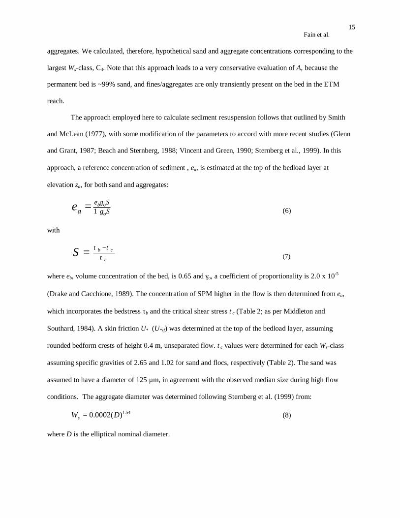
The approach employed here to calculate sediment resuspension follows that outlined by Smith
and McLean (1977), with some modification of the parameters to accord with more recent studies (Glenn
and Grant, 1987; Beach and Sternberg, 1988; Vincent and Green, 1990; Sternberg et al., 1999). In this
approach, a reference concentration of sediment , εa, is estimated at the top of the bedload layer at
elevation za, for both sand and aggregates:
SS
a o
obγγεε += 1 (6)
with
c
cbS τττ −= (7)
where εb, volume concentration of the bed, is 0.65 and γo, a coefficient of proportionality is 2.0 x 10⁻⁵
(Drake and Cacchione, 1989). The concentration of SPM higher in the flow is then determined from εa,
which incorporates the bedstress τb and the critical shear stress τc (Table 2; as per Middleton and
Southard, 1984). A skin friction U* (U*sf) was determined at the top of the bedload layer, assuming
rounded bedform crests of height 0.4 m, unseparated flow. τc values were determined for each Ws-class
assuming specific gravities of 2.65 and 1.02 for sand and flocs, respectively (Table 2). The sand was
assumed to have a diameter of 125 µm, in agreement with the observed median size during high flow
conditions. The aggregate diameter was determined following Sternberg et al. (1999) from:
54.1)(0002.0 DWs = (8)
where D is the elliptical nominal diameter.
Fain et al.16
Inverse Analysis Method
The purpose of the inverse analysis is to represent each observed SPM profile (as determined
from ABS) as a sum of profiles for the four settling classes C1 to C4. Each settling class profile is in turn
determined by a solution to the modified Rouse balance (4), using a U* determined by ambient conditions.
The inverse analysis is implemented using a non-negative least squares algorithm (Lawson and Hanson,
1974). The output of this inverse analysis is a value for each dimensional scaling concentration, C1i, for
each time and station, providing profiles of C1 to C4 concentrations throughout the water column.
Methodological details and verification of the inverse analysis are described in Fain (2000). Examples of
the inverse analysis results are shown in Figs. 4 and 5. Low-passed versions of the modeled washload
(C1) and ETM material (C2+C3+C4-sand) are shown in Fig. 6 for all stations. Sand has been excluded
from the ETM material because it does not participate in ETM ecodynamics.
C1 to C4 contained, respectively, an average of 4.4 %, 26.4 %, 35.6 %, 33.6 % of the total mass in
the Owen Tube analysis. The comparable percentages of the results of the inverse analysis results were
2.5 %, 28.3 %, 24.0 %, 45.2 % (moored ADP bottom bins). Thus, there is close agreement between the
Owen Tube and the inverse analysis regarding the total near-bed percentage of fines (for classes C1 and C2
individually) and aggregates plus sand (for classes C3 + C4 together). This agreement between the Owen
Tube and the inverse analysis for the fine settling classes likely reflects the relatively uniform distribution
in the vertical of C1 and C2. The inverse analysis over-estimates the amount of C4, even though the bottom
ADP bin is above the nominal Owen Tube depth. There are several possible reasons for this disagreement
for classes C3 and C4: a) uncertain and variable Owen Tube depth, especially during periods of strong
currents when C3 and C4 concentrations are large, b) systematic bias produced by the presence of both
sand and aggregates in C4, c) uncertainties in the near-field corrections for the ABS (Fig. 4a), and d) the
size dependence of the acoustic response to particles in a near Rayleigh scattering regime. Nonetheless,
the inverse analysis results provide a measure of Ws-class that is consistent in time and reasonably close to
the results found in Owen tube spectra. If sand rather than aggregates were the dominant material in C4,
Fain et al.17
the inverse analysis and the Owen tube results would likely have been more divergent, because of the
very strong acoustic response to sand.
Residence Time Index
A residence time index (RT) was developed in order to understand SPM retention time in the
system. RT calculations were carried out for each channel and the system as a whole. The SPM inventory
in the ETM (water column only) was estimated from inverse analysis results (with the ETM volume
defined in Fig 2). The predicted fluvial SPM supply is shown in Fig. 6a. RT is only an index rather than a
true residence time, because the volume of material stored on the bed cannot be determined, and because
the system is not in a steady state. RT is most useful on spring tides, when the entire inventory of SPM is
eroded from the bed.
Methodological Concerns
One potential concern in the use of ABS for the measurement of SPM concentration is the
presence in the ETM region of a large population of zooplankton with a size range similar to that of large
aggregates (500-1,500 µm). We cannot exclude occasional contamination of our results by backscatter of
biological origin, but epibenthic organisms typical of the ETM are relatively weak scatterers (Stanton et
al., 1988). Systematic LMER investigations (Morgan et al., 1997) of the temporal and spatial distribution
of zooplankton also suggest that biological contamination of the backscatter signal is a minor factor in the
present data set.
The SPM vs. OBS calibration was carried out using a pump oriented at a 90º angle to the flow (by
“transverse suction”; Bosman et al., 1987). This approach can lead to an undersampling of particulates
(especially sand), because the inertia of the sediment particles differs from that of the water entrained into
the sampling apparatus (Sundborg, 1956). Because the relative density of aggregates is much less than
that of sand, it is likely that undersampling of these particles is minimal. Moreover, the intake velocity at
the 51 mm diameter orifice was >4 ms-1, at least a factor of two greater than ambient flow velocity at any
Fain et al.18
time when the pump could be used (it could not be used near the surface during periods of maximum
ebb). Bosman et al. (1987) suggest that the efficiency of sand sampling should be ca. 80% under these
circumstances.
Finally, interpretation of the inverse analysis results must be carried out with the recognition that
SPM transport processes exhibit substantial across-channel variability that cannot be defined from the
moored instrument records. Stations Am012 and Am169 are located in the deepest part of the thalweg and
likely exhibit greater landward transport than seen elsewhere at these cross-sections. Ebb currents and
bank erosion are strong at Red26; vessel observations suggest that more landward transport occurs along
the north side of the South Channel at this location. Tansy is located at the outside of a curve, and
upstream bottom flow is absent except during neap tides. Extensive dredging between Tansy and AM169
suggests, however, that landward flow also occurs along the north side of the channel here.
Results
The output from the inverse analysis was a half-hourly time series of C1 to C4 profiles, in addition
to those for total SPM and along-channel velocity. For closer examination of neap-spring and seasonal
fluctuations, a low-pass Kaiser filter (Kaiser, 1974) was applied to all time series to remove the tidal
signal. The four moored stations provide extensive SPM data and, via the inverse analysis, Ws-class
distributions as a function of time. These results, augmented by vessel and auxiliary data, allow us to
investigate the amount and composition of SPM supplied to, contained in, and exported from the ETM.
Examination of these patterns provides insight into ETM processes on time scales from subtidal to
seasonal.
Seasonal and Tidal Monthly Patterns
It is convenient to consider seasonal and tidal monthly variability together, because the length of
the available time series is not sufficient to cleanly separate these time scales, and because processes on
the two scales interact. Seasonal variations in SPM concentrations and fluxes are driven primarily by river
Fain et al.19
flow, either directly or through the influence of river flow on estuarine circulation (Figs. 5-7). SPM
variability at tidal monthly scales (15-28 d) is also affected by natural river flow fluctuations, at periods of
less than a month, as well as by a weekly power-peaking cycle related to hydroelectric operations. The
strongest spring tides occur in mid-summer and mid-winter, but river flow as well as tidal currents
influence total bedstress. Maximum bedstresses occurred during the spring freshet (~d. 130), with a
secondary peak at about d. 230 (Fig. 8).
River flow and sediment supply was unusually high in 1997, because of high precipitation and
formation of a very large snowpack during the winter of 1996-1997. The spring freshet of 1997 occurred
from late April to mid-June with flows of 13 to 17 x 103 m3 s-1 (Fig. 7). The influence of large snow pack
extended throughout the summer and fall. Thus, minimum seasonal flow was 3,849 m3 s-1, >30% above
the usual fall minimum of 2,500-3,000 m3 s-1. The SPM input to the system was also very high in 1997,
because sediment transport varies strongly with river flow QR; i.e., as ~QR2.5 (Jay and Naik, 2000).
The maximum fluvial sediment supply during the study occurred during the spring freshet and
was 2.5 x 10³ kg s-1; maximum sand transport was 1.3 x 10³ kg s-1 (Fig. 7). Maximum fluvial SPM
concentrations were ~70mg l-1 (Fig. 6a). The total SPM supplied during the March to June period was
12.7 x 10⁶ t, out of the total water-year supply of 18.3 x 10⁶ metric tons. Considerable SPM was also
supplied by a high flow period in early January with the highest daily flows of the year (~20,000 m3 s-1).
The degree to which material supplied during winter 1996-97 affected SPM dynamics during the May to
December 1997 period is unknown, but the following analyses suggest that a pulse of SPM from the river
exerts an influence on SPM dynamics for several months.
The strength of the spring freshet flow is very evident in the ADP velocity records (not shown).
Upstream bottom flow at all the South channel stations was weak or absent before ca. d 180. Total SPM
determined from ABS and concentrations of C3 and C4 (Figs. 5, 6b, 6c) were maximal during and after the
spring freshet, generally following the seasonal river flow and predicted SPM supply patterns shown in
Fig. 7. Thus, the SPM time history indicates a limited residence time for SPM in the system, as well as a
close linkage between the river and estuary. The time series of total transport for all stations supports H1
Fain et al.20
by demonstrating that SPM supplied during the spring freshet is exported primarily by spring tides,
during and for about a month after the spring freshet (Fig. 9).
Still, high SPM concentrations and export events continue into July and August, 30-60 d after the
flow decreased to summer levels, indicating substantial storage in the system (Figs. 5, 6, 9). Total and Ws-
class SPM show, moreover, strong neap-spring (tidal monthly) fluctuations not seen in the SPM supply
(Fig. 6a), also suggesting temporary estuarine storage of SPM. Given that accumulation of fines in the
deeper channels is minimal due to strong currents, it is likely that high spring tide SPM values after the
freshet result from storage of fines in peripheral areas, an idea we will return to below.
The seasonal location of the ETM in the Columbia River estuary is evident from examination of
the distribution of material trapped in the ETM, over time at the various stations (Fig 6b, 6c). We focus
first on processes in the South channel, where multiple stations make the influence of river flow on ETM
position and concentrations evident. Until the end of the spring freshet at ~d 170, concentrations of the
trapped material are at a seasonal maximum at all three South channel stations, but greatest at Tansy. This
is consistent with shipboard observations that the ETM was centered near Tansy, but advected tidally
from Red26 to Am169. As the flows decrease (d 170 to d 280), the order of concentrations is (from high
to low): Am169, Tansy, and Red26. This pattern is consistent with the expected seasonal pattern of
landward ETM migration to the vicinity of Am169.
In a normal flow year, the ETM would be found landward of Am169 from about August to
October, but it is doubtful that this occurred, given the relatively high flows during summer and fall 1997.
At the end of the record, there is an increase in the concentration of trapped material at Tansy, but not at
Red26. This may be indicative of an increase in supply of sediment from lower river tributaries, not
included in the flow time series of Fig. 7, or it may indicate increased resuspension from tributary bays
due to storms. Finally, SPM concentrations at Red26 may be influenced by the near-mouth ETM, about
which little is known. That these patterns of ETM movement are subtle is a consequence of the multiple
ETM and of the fact that all three stations are within the tidal excursion of at least one ETM throughout
the time period.
Fain et al.21
One of the most dramatic features of the low passed concentration records is that the highest SPM
concentrations are found throughout the record at the North channel station, Am012 (Fig. 6c). Strong
ETM trapping in the North channel is analogous to salt transport patterns in the system. Salt is transported
landward under most hydrographic conditions in the North channel (Hughes and Rattray, 1980; Jay and
Smith, 1990; Kay et al., 1996), whereas salt transport in the South channel is consistently seaward.
Inferred, but unmeasured, is a salt transfer across the mid-estuary flats via shallow channels that trend
southeast (landward) from station Am012. Landward SPM transport is consistent and strong near the bed
in the North channel (Fig. 9d). During the spring freshet, Am012 is the only station that shows any
landward bottom SPM transport, while surface transport at Am012 is only weakly seaward throughout
most of the record. Even allowing for seaward transport elsewhere in the section, it is likely that there is
net landward SPM transport at this cross-section. Unlike salt, however, most SPM transport occurs in the
thalweg, and SPM is not likely transferred from the North to the South channel. This allows larger
particles to accumulate in the North channel, with possible long-term storage in the two adjacent
peripheral bays that are known to be accreting (Sherwood et al., 1990).
Seasonal changes in system-scale SPM transport patterns are summarized in Fig. 10, which
shows net transport at all four ADP stations on two spring tides, one during and one shortly after the
spring freshet. The transport during the spring freshet spring tide is seaward at all stations (Fig. 10a), with
strongest transport at Red26. Export of SPM continues in the South channel, ~30 days after the spring
freshet ended, but transport is strongly landward at Am012 (Fig. 10b). The landward flux at Am012 is
likely supported by release of SPM from peripheral bays and recirculation from the South channel to the
North channel. Taken together, the results shown in Figs. 9-11 shows the export of SPM on spring tides
during and after the freshet (H1) and suggests that storage in peripheral bays may be important.
The distribution of SPM between the Ws-classes also provides information on ETM dynamics.
Fig. 5 shows inverse analysis results for the North channel station, Am012. All Ws-classes demonstrate
neap-spring and seasonal fluctuations in concentrations. The smaller Ws- classes (particularly C2) show
substantial concentrations at the surface, especially during and after the spring freshet (up to d 170). There
Fain et al.22
is also a shift in the composition of the coarser material from C3 during the freshet to C4 after the freshet.
This shift is not related to sand concentrations and may indicate the formation of larger aggregates after
the spring freshet. Whether this shift in composition is related to biological activity or a change in the
character of the sediment supplied is unclear. The South channel stations are dominated by C4 throughout.
The smallest Ws-class (C1, 0.014 mm s-1) is essentially washload in the channel environments
represented by all the ADP stations. Accordingly, C1 concentrations are similar throughout the record for
all stations, except that they are low at Red26 during and after the spring freshet. Substantial neap-spring
variations of C1 at all stations suggest that this material is being stored somewhere in the estuary on neap
tides. The higher washload concentrations at Am169, Tansy, and Am012 may indicate the influence of
peripheral bays, primarily Youngs Bay and Grays Bay.
SPM Residence Time Index
We quantify the retention of SPM by the system and consider H2 using the residence time index,
RT (Fig. 11). Unlike salt (a conservative scalar), SPM settles. Only the maximum RT during spring tides is
meaningful – during most of the tidal month, much of the inventory of sediment is stored on the bed or in
peripheral bays. The total RT (for the North and South Channels together) suggests that sediment storage
is small (less than 14 d) during the spring freshet -- most of the SPM brought into the estuary is exported
at the latest on the next spring tide. The situation is different after the freshet. Maximum RT values are of
the same order as the time since the freshet, suggesting that material from the freshet is retained in the
system on seasonal time scales. Given that there is essentially no storage of fine sediments on the bed
during spring tides, it is likely that material is stored in peripheral bays. Mid-estuary sand flats are another
possible storage site, but their ability to store fines is limited because they are wave-swept during most
seasons. This is reflected in the high sand content of their bed material.
A question we cannot address directly here is the rate and timing of export from peripheral bays
to the ETM. The maximum inventory of SPM in the ETM (the maximum value of the numerator of RT) is
~1.5 kg m-2, sufficient to create, upon deposition, a layer in the ETM channels only 5 to 10 mm thick
Fain et al.23
(assuming an initial bulk SPM density of 180 to 270 kg m-3; Winterwerp et al., 1993). This is consistent
with the fact that sand is always dominant in channel grab samples. Still, thin layers of surficial fines are
sometimes captured. We cannot rigorously distinguish, therefore, between continuous supply from the
flats and episodic supply during storms and spring tides, but supply to the channel during periods of
strong bed stress seems likely.
Rouse Number, Trapping Efficiency and the Importance of Advection
Rouse number P is an important descriptor of ETM processes. H5 postulates (following Jay et al.,
2000) that SPM with intermediate P values is most effective at trapping SPM in an ETM. Material that
settles too slowly is washload. Material that settles too rapidly remains permanently on the bed or moves
only as bedload. This suggests that the ETM material adjusts to ambient bedstresses. To test this idea, we
have plotted low passed tidal number P4 as a function of time for Am012 and Am169 (Figs. 13a, 13b).
This value of P4 is obtained using the minimum U* observed as a moving 6 hr. window, the result then
being low passed to remove fluctuations on time scales < 25 hours. Results show that P4 is between ~1.2
and 2 at ETM stations, except during export events, when it is slightly lower and the weakest neaps, when
it is >2. Since P3 is smaller than P4 by a factor of seven, it seems unlikely that material could be trapped at
all without the formation of aggregates.
Hypothesis H3 addresses tidal monthly variations in advection, as represented by low passed
(subtidal) A. Consistent with H3, tidally-averaged values of A are almost always greater on neap than on
spring tides at all the stations, and spring-neap differences in A are greatest at Red26 during the high-flow
season, when stratification is maximum (Fig. 13a). Vessel observations also regularly show mid-depth
SPM maxima associated with the velocity maximum at the top of the intruding salt wedge. High
bedstresses near the mouth of the estuary are more capable of suspending material than is the case in the
ETM itself, an important factor on neap tides. Finally, note that the spring-neap differences in A shown
here are, in fact, conservative, because the bottom ADP bin is 2 to 3 meters off the bed. This effectively
puts a floor on Hm at the level of the lowest bin and causes fluctuations below this level to be missed.
Fain et al.24
During periods of strong bedstress when local erosion and deposition rather than advection are dominant,
the SPM maximum is at the bed, and Hm should be less than the value calculated from the ADP data.
The relative values of A at the various moorings in the South Channel also provide information
regarding ETM processes (Fig. 13a). Red26 has the highest advection numbers in the spring,
corresponding with highly stratified conditions at this station. During this period, the mean ETM position
is located near Tansy, and high A values at Red26 correspond to advection of SPM from seaward of
Red26 toward the ETM. Am169 has higher advection numbers during summer and early fall, indicating
an ETM at or landward of this station, consistent with the discussion of Fig. 6. Tansy has highest A values
in the late fall, which may correspond with a seaward movement of the ETM back toward Tansy.
Hypothesis H4 addresses the seasonal variations and spatial heterogeneity of trapping efficiency,
as quantified by E. We show in Fig. 13b the E time series for the three stations most frequently in the
center of the ETM: Am169, Am012 and Tansy. Neap tides are characterized by low E values, because
SPM is accumulated near the bed and in peripheral bays at this time. The high E values observed on
spring tides reflect accumulation of sediment during the previous neap. E is clearly variable in space; the
North channel station Am012 consistently shows the highest E values, despite the fact that SPM supply to
the North Channel is largely indirect. It is evident in Fig. 14 that all three stations show an inverse
relationship between E and river flow QR. E is maximal during low-moderate flow periods and exhibits
spatial heterogeneity, consistent with H4. We cannot be certain what values of E would have occurred
under normal seasonal low flows, because there were no really low flows during the sampling period.
Conclusions about E are indirect, moreover, because of lags built into the system. E was maximal as the
flow fell after the freshet, in part due to storage of SPM in peripheral bays. We cannot directly answer
questions regarding the efficiency of the trapping processes in the ETM itself.
Conclusions
The purpose of the work described here was twofold: a) to develop new methods to measure
ETM processes, and b) to understand ETM dynamics of time scales from subtidal to seasonal. The broad
Fain et al.25
range of time scales involved in understanding ETM processes dictated use of moored instrumentation.
Acoustic backscatter (ABS) from Doppler profilers provides a consistent measure of SPM concentrations,
but considerable effort is required to calibrate the ABS signal and interpret it in terms of Ws-classes via an
SPM profile model and inverse analysis. Vessel data are required for calibration, verification, and
interpretation.
Five hypotheses regarding ETM processes (H1 to H5) were developed. Results support H1: SPM
is exported from the Columbia River estuary primarily on spring tides during and shortly after the spring
freshet, as evidenced in the total transport and SPM time histories for each station. The evidence also
supports H3. Elevated values of A indicate that advection is more important on neap tides than spring
tides. Furthermore, values of low passed, tidal maximum Rouse number P for large aggregates were
typically between 1.2 and 2, but were <1.2 during periods of SPM export. This is consistent with the idea
that only SPM adjusted to ambient hydrodynamic forcing (i.e., falling within a fairly narrow range of P
values) can be efficiently trapped in an ETM (H5).
Time series of E suggest the most effective trapping occurs during neap tides with low-moderate
river flow, supporting H4 with two qualifications: a) no really low flows occurred in the time period of
observations, and b) E is determined in part by lateral supply from peripheral bays, a process not
necessarily correlated with river flow. The high sediment concentrations after the spring freshet and plots
of residence time index RT provide evidence for storage of SPM in peripheral bays on both tidal monthly
and seasonal scales (H2). Particle trapping was also more effective in the North channel, despite its
indirect SPM supply. These factors render results regarding H4 somewhat ambiguous. Longer records and
data from peripheral bays are needed to truly resolve H4.
The joint use of moored acoustic and cruise data provides unprecedented temporal and spatial
resolution of sediment dynamics. This approach to estuarine sediment dynamics should have broad utility
beyond the system considered here. The results of similar analyses could be applied to science and policy
issues related to dredging, dredged material disposal, pollutant dispersion, and estuarine management.
Fain et al.26
Symbols
A advection number
Ci volume sediment concentration of the thi settling velocity class
C1i volume sediment concentration at the first bin for class i
Cd drag coefficient
Cm maximum SPM concentration
Cs source SPM concentration
D elliptical nominal diameter
E Trapping Efficiency
sK mass diffusivity for suspended sediment
H total depth
Hm height of maximum sediment concentration
Ls horizontal SPM length scale
P Rouse parameter
RT Residence Time index
U along-channel velocity
<U> mean along-channel velocity
*U shear velocity
U*sf skin friction velocity
TU tidal velocity scale
sW Settling velocity
i Ws class indicator
j bin number
k Von Karman's constant, = 0.408
Fain et al.27
m number of Ws classes
n number of depth bins for analysis
t time
u ,v , w alongchannel, lateral and vertical velocities
ω semidiurnal frequency scalar
x , y , z alongchannel, lateral and vertical coordinates
z1 height of the first ADP bin
za height of the bedload layer
γ0 coefficient of proportionality (empirical resuspension parameter)
∆U surface along-channel velocity minus bottom along channel velocity
εa sediment concentration at the height of the bedload, za
εb volume concentration in bed, = 0.65 (assuming a porosity of 0.35)
π acceleration term in non-dimensional transport equation
σ non-dimensional distance from bed
τb bed shear stress
τc critical shear stress
Acknowledgments
This work was funded by the Office of Naval Research through grant N00014-97-1-0012 and AASERT
grant N00014-97-1-0625 (the latter supported the graduate work of Annika Merle Virginia Fain), the
National Science Foundation Grant Columbia River Land-Margin Ecosystem Research Project, OCE-
9412928, and a National Science Foundation SGER, Amplification of El Niño-Southern Oscillation
(ENSO) Climate Effects in Estuaries, OCE-9816083. We thank Dr. Denise Reed of Louisiana State
University for providing the LMER settling velocity data set for 1997 and Dr. Fred Prahl of Oregon State
University for the LMER pumped OBS calibration data set.

Fain et al.28
Literature Cited
Allen, G.P., J.C. Salomon, P. Bassoullet, Y. Du Pehoat, and C. De Grandpre. 1980. Effects of tides on
mixing and suspended sediment in macrotidal estuaries. Sedimentary Geology 26: 69-80.
Baptista, A.M., M. Wilkin, P. Pearson, P. Turner, C. McCandlish, and P. Barrett. 1999. Coastal and
Estuarine Forecast Systems: A Multi-Purpose Infrastructure for the Columbia River. Earth System
Monitor 9: 1-5.
Baptista, A.M., M. Wilkin, P. Pearson, P. Turner, C. McCandlish, P. Barrett, S. Das, W. Sommerfield, M.
Qi, N. Nangia, D. Jay, D. Long, C. Pu, J. Hunt, Z. Yang, E. Myers, J. Darland and A. Farrenkopf. 1998.
Towards a Multi-Purpose Forecast System for the Columbia River Estuary. Ocean Community
Conference '98, Baltimore, MD. pp. 1-6.
Barans, C.A., B.W. Sterner, D.V. Holliday, and C.F. Greenlaw. 1997. Variation in the vertical
distribution of zooplankton and fine particles in an estuarine inlet of South Carolina. Estuaries 20: 487-
482.
Baross, J. A., B. Crump, and C. A. Simenstad. 1994. Elevated 'microbial loop' activities in the Columbia
River estuary turbidity maximum. In Changes in Fluxes in Estuaries, K.R. Dyer and R.J. Orth, eds,
Frendesborg, Denmark: Olsen and Olsen. pp. 459-464.
Beach, R.A. and R.W. Sternberg. 1988. Suspended sediment transport in the surf zone: response to cross-
shore infragravity motion. Marine Geology 80: 61-79.
Fain et al.29
Bokuniewicz, H. and C.L. Arnold. 1984. Characteristics of suspended sediment transport in the lower
Hudson River. Northeastern Environmental Science 3: 184-189.
Bosman, J.J., E.T.J.M. van der Velden, and C. H. Hulsbergen. 1987. Sediment concentration
measurement by transverse suction. Coastal Engineering 11: 353-370.
Crump, B.C. and J.A. Baross. 1996. Particle-attached bacteria and heterotrophic plankton associated with
the Columbia River estuarine turbidity maxima. Marine Ecology Progress Series 138: 265-273.
Drake, D.E. and D.A. Cacchione. 1989. Estimate of the suspended sediment reference concentration (Ca)
and resuspension coefficient (γ0) from near-bottom observations on the California shelf. Continental Shelf
Research 9(1): 51-64.
Fain, A.M.V. 2000. Suspended Particulate Dynamics in the Columbia River Estuary. Masters thesis.
Portland, OR: Oregon Graduate Institute.
Flagg, C.N. and S.L. Smith. 1989. On the use of the acousitc Doppler current profiler to measure
zooplankton abundance. Deep-Sea Research 36(3): 455-474.
Gelfenbaum, G. 1983. Suspended-sediment response to semidiurnal and fortnightly tidal variations in a
mesotidal estuary: Columbia River, USA. Marine Geology 52: 39-57.
Giese, B.S and D.A. Jay. 1989. Modeling tidal energetics of the Columbia River Estuary. Estuaries,
Coastal and Shelf Science 29: 549-571.
Fain et al.30
Glenn, S.M. and W.D. Grant. 1987. A suspended sediment stratification correction for combined wave
and current flows. Journal of Geophysical Research 92(C8): 8244-8264.
Grabemann, I. and G. Krause. 1989. Transport processes of suspended matter derived from time series in
a tidal estuary. Journal of Geophysical Research 94: 14373-14379.
Green, M.O., R.G. Bell, T.J. Dolphin, A. Swales. 2000. Silt and sand transport in a deep tidal channel of a
large estuary (Manukau Harbour, New Zealand). Marine Geology 163: 217-240.
Hanes, D.M., C.E. Vincent, D.A. Huntley, and T.L Clarke. 1988. Acoustic measurements of suspended
sand concentration in the C2S2 experiment at Stanhope Lane, Prince Edward Island. Marine Geology 81:
185-196.
Holdaway, G.P. and P.D. Thorne. 1997. Determination of a fast and stable algorithm to evaluate
suspended sediment parameters from high resolution acoustic backscatter systems. In 7th International
Conference on Electronic Engineering in Oceanography, Piscataway, NJ: IEEE. pp. 86-92.
Hughes, F.W. and M. Rattray. 1980. Salt flux and mixing in the Columbia River estuary. Estuarine and
Coastal Marine Science 10: 479-492.
Jay, D.A., W.R. Geyer and D.R. Montgomery. 2000. An ecological perspective on estuarine
classification. In Estuarine Science, A Synthetic Approach to Research and Practice, J.E. Hobbie, ed,
Washington DC: Island Press. pp. 149-176.

Fain et al.31
Jay, D.A. and J.D. Musiak. 1994. Particle trapping in estuarine tidal flows. Journal of Geophysical
Research 99: 20445-20461.
Jay, D. A., P.M. Orton, D.J. Wilson, A.M.V. Fain and J. McGinity. 2001. Particle trapping in Stratified
estuaries -- definition of a parameter space, submitted to Continental Shelf Research.
Jay, D.A. and P. Naik. 2000. Climate effects on Columbia River sediment transport. In Southwest
Washington Coastal Erosion Workshop Report 1999, US Geological Survey Open File Report, G.
Gelfenbaum and G. Kaminsky, eds.
Jay, D.A. and J.D. Smith. 1990. Circulation, density distribution and neap-spring transitions in the
Columbia River Estuary. Progress in Oceanography 25: 81-112.
Kay, D. J., D.A. Jay and J.D. Musiak. 1996. Salt transport through an estuarine cross-section calculated
from moving vessel ADCP and CTD data Buoyancy Effects on Coastal and Estuarine Dynamics. In
Buoyancy Effects on Coastal and Estuarine Dynamics, D.G. Aubrey and C. Friedrichs, eds, Washington
DC: AGU. pp. 195-212.
Kaiser, J.F. 1974. Non-recursive digital filter design using the lo-sinh window function. In Proceedings of
1974 IEEE Symposium on Circuits and Systems, Piscataway, NJ: IEEE. pp. 20-23.
Kineke, G.C. and R.W. Sternberg. 1989. The effect of particle settling velocity on computed suspended
sediment concentration profiles. Marine Geology 90: 159-174.
Kineke, G.C. and R.W. Sternberg. 1992. Measurements of high concentration suspended sediments using
the optical backscatterance sensor. Marine Geology 108: 253-258.
Fain et al.32
Lawson, C.L. and R.J. Hanson. 1974. Solving Least Square Problems. Englewood Cliffs, New Jersey:
Prentice-Hall.
Lee, H.L. and D.M. Hanes. 1995. Direct inversion method to measure the concentration profile of
suspended particles using backscattered sound. Journal of Geophysical Research 100: 2649-2657.
Lee, H.L. and D.M. Hanes. 1996. Comparison of field observations of the vertical distribution of
suspended sand and its prediction by models. Journal of Geophysical Research 101: 3561-3572.
Libicki, C., K. Bedford, and J. Lynch. 1989. The interpretation and evaluation of a 3-MHz acoustic
backscatter device for measuring benthic boundary layer sediment dynamics. Journal of Acoustical
Society of America 85: 1501-1511.
Long, C.E. 1981. A simple model for time-dependent stably stratified turbulent boundary layers. Ph.D
Thesis. Seattle, WA: University of Washington, Department of Oceanography.
LMER Coordinating Committee (Boynton, W., J.T. Hollibaugh, D. Jay, M. Kemp, J. Kremer, C.
Simenstad, S.V. Smith, and I. Valiela). 1992. Understanding changes in coastal environments: the Land
Margin Ecosystems Research Program. EOS 73: 481-485.
Lucas, L.V., J.K. Thompson, J.R. Koseff, and S.B. Monismith. 1999. Processes governing phytoplankton
bloom in estuaries--Part I, The role of horizontal transport. Marine Ecology Progress Series 187: 1-16.
Ludwig, K.A. and D.M. Hanes. 1990. Laboratory evaluation of optical backscatterance suspended solids
sensors exposed to sand-mud mixtures. Marine Geology 94: 173-179.
Fain et al.33
Lynch, J.F. 1985. Theoretical analysis of ABSS data for Hebble. Marine Geology 66: 277-289.
Lynch, J.F. and Y.C. Agrawal. 1991. A model-dependent method for inverting vertical profiles of
scattering to obtain particle size spectra in boundary layers. Marine Geology 99: 387-401.
Lynch, J.F., T.F. Gross, B.H. Brumley, and R.A. Filyo. 1991. Sediment concentration profiling in
HEBBLE using a 1-MHz acoustic backscatter system. Marine Geology 99: 361-385.
Lynch, J.F., J.D. Irish, C.R. Sherwood, and Y.C. Agrawal. 1994. Determining suspended sediment
particle size information from acoustical and optical backscatterance measurements. Continental Shelf
Research 14: 1139-1165.
Middleton, G.V. and J.B. Southard. 1984. Mechanics of Sediment Movement. Tulsa, OK: Society of
Economic Paleontologists and Mineralogists.
Morgan, C.A., J.R. Cordell, and C.A. Simenstad. 1997. Sink or swim? Copepod population maintenance
in the Columbia River estuarine turbidity maxima region. Marine Biology 129: 309-317.
Nichols, M.M. and R.B. Biggs. 1985. Estuaries. In Coastal Sedimentary Environments, Davis R.A., Jr.,
ed, New York, NY: Springer-Verlag. pp. 77-186.
Nowell, A.R.M. 1983. The benthic boundary layer and sediment transport. Reviews in Geophysics and
Space Physics 21: 1181.
Fain et al.34
Reed, D.J. and J. Donovan. 1994. The character and composition of the Columbia River estuarine
turbidity maximum. In Changes in fluxes in Estuaries, K.R. Dyer and R.J. Orth, eds, Fredensborg,
Denmark: Olsen and Olsen. pp. 445-450.
Schaffsma, A.S. and A.E. Hay. 1997. Attenuation in suspensions of irregularly shaped sediment particles:
A two-parameter equivalent spherical scatterrer model. Journal of Acoustical Society of America 102:
1485-1502.
Sherwood, C.R. and J.S. Creager. 1990. Sedimentary geology of the Columbia River Estuary. Progress in
Oceanography 25: 15-79.
Sherwood, C.R., D.A. Jay, R.B. Harvey, P. Hamilton, and C.A. Simenstad. 1990. Historical changes in
the Columbia River Estuary. Progress in Oceanography 25: 299-352.
Simenstad, C.A., D.A. Jay, and C.R. Sherwood. 1992. Impacts of watershed management on land-margin
ecosystems: the Columbia River Estuary as a case study. In New Perspectives for Watershed
Management - Balancing Long-term Sustainability with Cumulative Environmental Change, R. Naimen,
ed, New York, NY: Springer-Verlag. pp. 266-306.
Simenstad, C.A., D.J. Reed, D.A. Jay, J.A. Baross, F.G. Prahl and L.F. Small. 1994. Land-margin
ecosystem research in the Columbia River estuary: investigations of the couplings between physical and
ecological processes within estuarine turbidity maxima. In Changes in fluxes in Estuaries, K.R. Dyer and
R.J. Orth, eds, Fredensborg, Denmark: Olsen and Olsen. pp. 437-444.
Fain et al.35
Simenstad, C.A., L.F. Small, C.D. McIntire, D.A. Jay, and C. Sherwood. 1990. Columbia River Estuary
studies: An introduction to the estuary, a brief history, and prior studies. Progress in Oceanography 25: 1-
13.
Smith, J.D. and S.R. McLean. 1977. Spatially averaged flow over a wavy surface. Journal of Geophysical
Research 82: 1735-1746.
Smith, S.V., J.T. Hollibaugh, S.J. Dollar, and S. Vink. 1991. Tomales Bay metabolis: C-N-P
stoichiometry and ecosystem heterotrophy at the land-sea interface. Estuarine, Coastal and Shelf Science
33: 223-57.
Sommerfield, W.N. 1999. Variability of residual properties in the Columbia River Estuary: pilot
application of emerging technologies. Master's thesis. Portland, OR: Oregon Graduate Institute of Science
and Technology.
Stanton, T.K., D. Chu, and P.H. Wiebe. 1998. Sound Scattering by Several Zooplankton Groups II:
Scattering Models. Journal of the Acoustical Society America 103: 236-253.
Sternberg, R.W., I. Berhane, and A.S. Ogston. 1999. Measurement of size and settling velocity of
suspended aggregates on the northern California continental shelf. Marine Geology 154: 43-53.
Sundborg, ? . 1956. The river Klarläven a study of fluvial process. Geograpfiska Annaler 2-3: 233-235.
Thevenot, M.M. and N.C. Kraus. 1993. Comparison of acoustical and optical measurements of suspended
material in the Cheasapeake Estuary. Journal of Marine Environmental Engineering 1: 65-79.
Fain et al.36
Thorne, P.D., C.E. Vincent, P.J. Hardcastle, S. Rehman, and N. Pearson. 1991. Measuring suspended
sediment concentrations using acoustic backscatter devices. Marine Geology 98: 7-16.
US Geological Survey. 1971. Distribution of Radionuclides in Bottom Sediments of the Columbia River
Estuary. Portland, OR: US Department of the Interior.
Vincent C.E. and M.O. Green. 1990. Field measurements of the suspended sand concentration profiles
and fluxes and of the resuspension coefficient γ0 over a rippled bed. Journal of Geophysical Research 94:
11591-11601.
Winterwerp, J.C., J.M. Cornelisse, and C. Kuijper. 1993. A laboratory study on the behavior of mud from
the Western Scheldt under tidal conditions. In Nearshore and Estuarine Cohesive Sediment Transport.
Washington DC: AGU. pp. 295-313.
Young, R.A., J.T. Merrill, T.L. Clarke, J.R. Proni. 1982. Acoustic profiling of suspended sediments in the
marine bottom boundary layer. Geophysical Research Letters 9(3): 175-178.
Fain et al.37
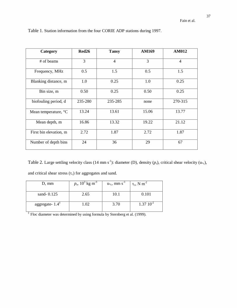
Table 1. Station information from the four CORIE ADP stations during 1997.
Category Red26 Tansy AM169 AM012
# of beams 3 4 3 4
Frequency, MHz 0.5 1.5 0.5 1.5
Blanking distance, m 1.0 0.25 1.0 0.25
Bin size, m 0.50 0.25 0.50 0.25
biofouling period, d 235-280 235-285 none 270-315
Mean temperature, °C 13.24 13.61 15.06 13.77
Mean depth, m 16.86 13.32 19.22 21.12
First bin elevation, m 2.72 1.87 2.72 1.87
Number of depth bins 24 36 29 67
Table 2. Large settling velocity class (14 mm s-1): diameter (D), density (ps), critical shear velocity (u*c),
and critical shear stress (τc) for aggregates and sand.
D, mm ps, 103 kg m-3 u*c, mm s-1 τc, N m-2
sand- 0.125 2.65 10.1 0.101
aggregate- 1.4‡ 1.02 3.70 1.37 10-2
‡ Floc diameter was determined by using formula by Sternberg et al. (1999).
Fain et al.38
Fig. 1. Schematic of an estuarine turbidity maximum, depicting the interactions between biological,
chemical, geological, and physical processes (from http://depts.washington.edu/cretmweb/CRETM.html).
Fig. 2. Map of CORIE moored ADP stations in the Columbia River Estuary for 1997. Red26 and Am169
had 0.5 MHz ADPs, while Tansy and Am012 had 1.5 MHz ADPs. The north and south channel ETMs are
depicted by red outlines (modified from Simenstad et al., 1990).
Fig. 3. An example of the acoustic backscatter (abs) nearfield (nfc) and farfield (ffc) corrections applied
to the 0.5 mHz ADP data before conversion to SPM concentration.
Fig. 4. Examples of inverse analysis fit using four Ws classes at: (a) Tansy (1.5 MHz) and (b) Am169 (0.5
MHz).
Fig. 5. Inverse analysis results: low pass filtered concentrations for all four Ws-classes at Am012, (a) near
the surface and (b) near the bed. Neap-spring fluctuations are evident in all Ws-classes, as well as seasonal
variations.
Fig. 6. (a) Estimated fluvial source material minus estimated sand, (b) low passed ETM trapped at South
channel stations, and (c) ETM trapped material at Am012. ETM trapped material consists of three Ws
classes (0.3 mm s-1, 2.0 mm s-1, and 14.0 mm s-1) minus predicted sand concentrations. Gaps in the SPM
record between ~d. 230 and 315 indicate biofouling of a duration that varied between stations.
Fig. 7. River inflow to the estuary (Qr) as measured by the US Geological Survey at Beaver, contrasted
against estimated total fluvial sediment load and estimated fluvial sand supply. The total load predictions
are the sum of predictions for the Columbia River at Vancouver, WA and the Willamette River at
Portland, OR. The sand transport estimate is for the Columbia at Vancouver only. The sand supply for
early January is greatly underestimated, because most of the flow at the time was from the Willamette and
other Lower Columbia river tributaries.
Fain et al.39
Fig. 8. Shear velocity, U*, at Tansy and river flow, QR, at Beaver army terminal during the investigation
period.
Fig. 9. Total non-tidal SPM transports at all CORIE stations for 1997, near-surface (�) and near-bed (∆).
Negative transports are seaward.
Fig. 10. Spring tide SPM transport patterns during the freshet (a) and after the freshet (b). The green
arrows refer to transport near the water surface and red arrows refer to transport near the bed.
Fig. 11. SPM residence time index in the Columbia River Estuary for the South channel ETM
(*), North channel ETM (+), and for the two channels together (∆). Residence time index was
not determined for periods where biofouling was present.
Fig. 12. Low pass filtered large aggregate Rouse number, P4, for Am012 (a) and Am169 (b).
Fig. 13. Low-passed advection number A for all South channel stations (a) and low passed trapping
efficiency (E) for Am169, Am012 and Tansy (b).
Fig. 14. Trapping Efficiency E vs. river flow Qr in m3 s-1 at Am012 (*), Tansy (+), and Am169(∆).
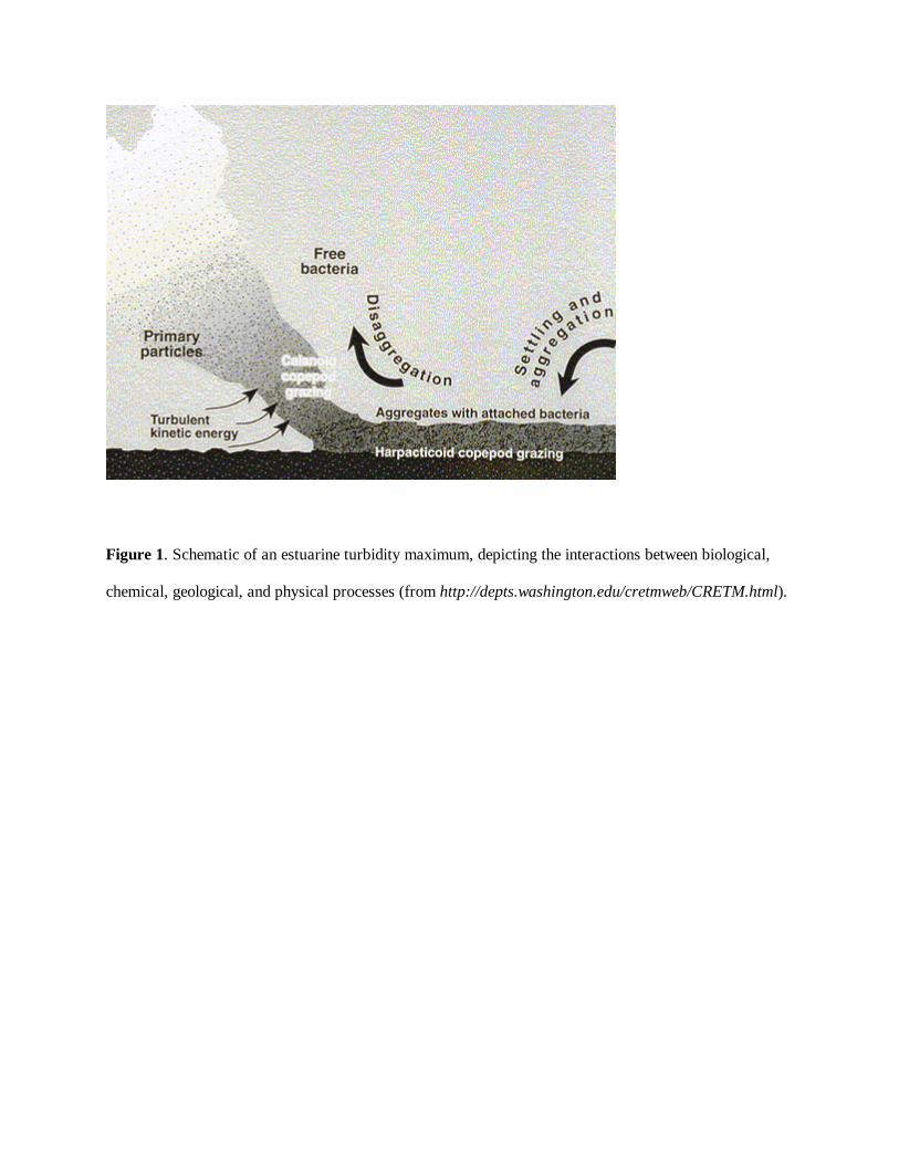
Figure 1. Schematic of an estuarine turbidity maximum, depicting the interactions between biological,
chemical, geological, and physical processes (from http://depts.washington.edu/cretmweb/CRETM.html).
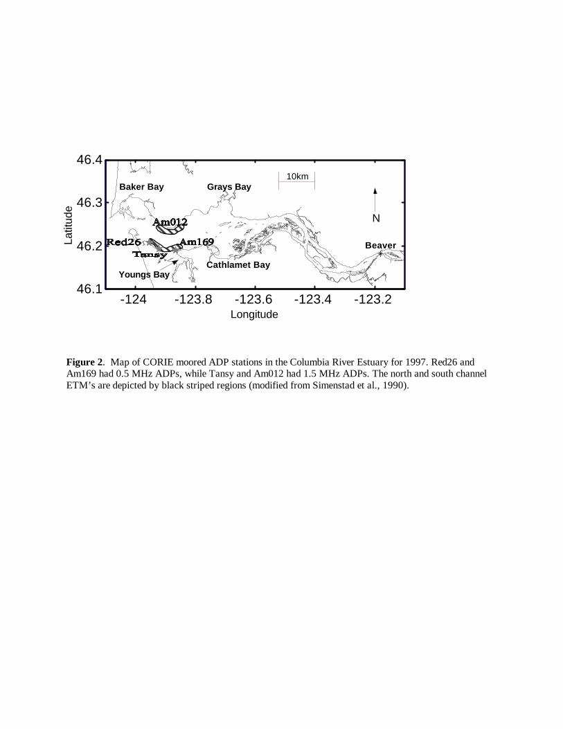
Figure 2. Map of CORIE moored ADP stations in the Columbia River Estuary for 1997. Red26 andAm169 had 0.5 MHz ADPs, while Tansy and Am012 had 1.5 MHz ADPs. The north and south channelETM’s are depicted by black striped regions (modified from Simenstad et al., 1990).
-124 -123.8 -123.6 -123.4 -123.246.1
46.2
46.3
46.4
Longitude
Latit
ude
Beaver
Youngs Bay
Baker Bay Grays Bay
Cathlamet Bay
10km
N
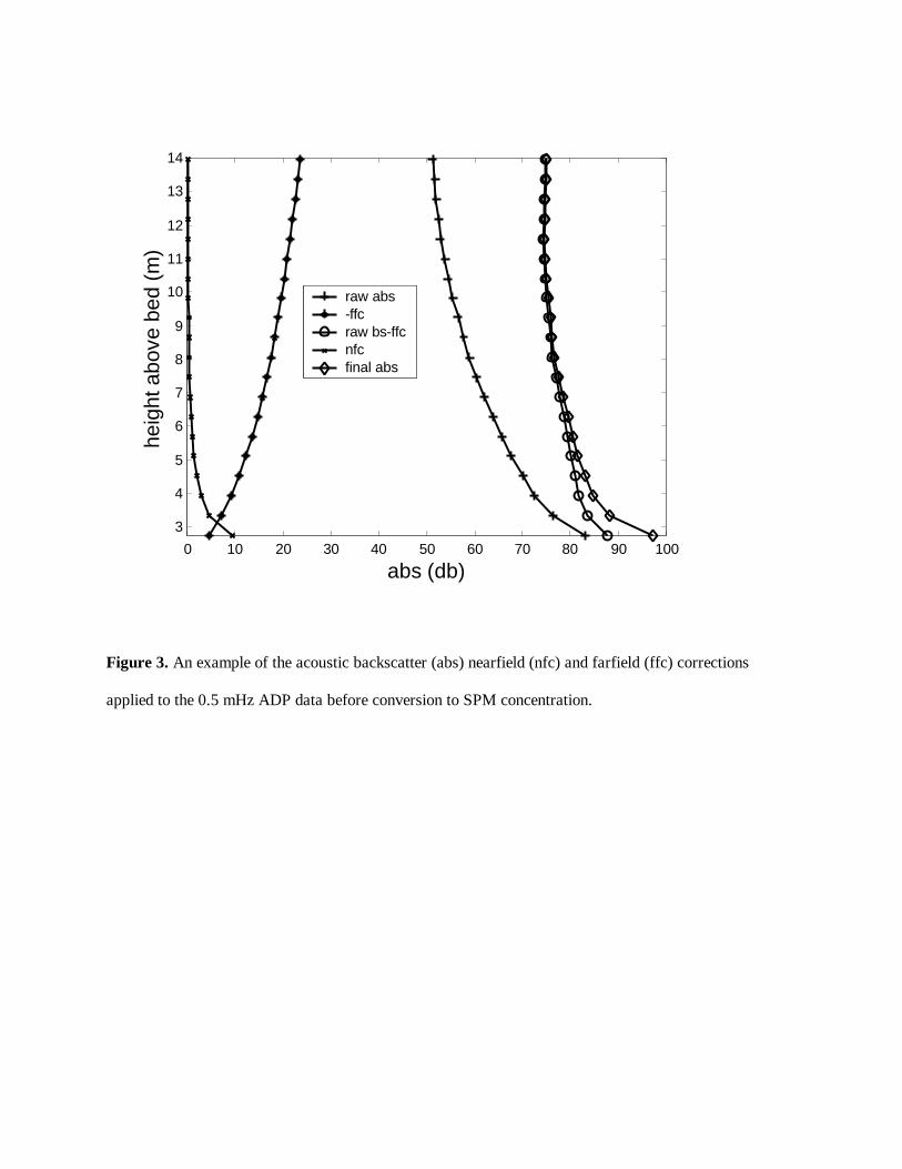
0 10 20 30 40 50 60 70 80 90 1003
4
5
6
7
8
9
10
11
12
13
14he
ight
abo
ve b
ed (m
)
abs (db)
raw abs -ffc raw bs-ffcnfc final abs
Figure 3. An example of the acoustic backscatter (abs) nearfield (nfc) and farfield (ffc) corrections
applied to the 0.5 mHz ADP data before conversion to SPM concentration.
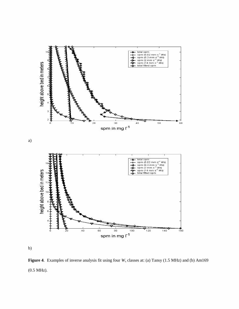
a)
b)
Figure 4. Examples of inverse analysis fit using four Ws classes at: (a) Tansy (1.5 MHz) and (b) Am169
(0.5 MHz).
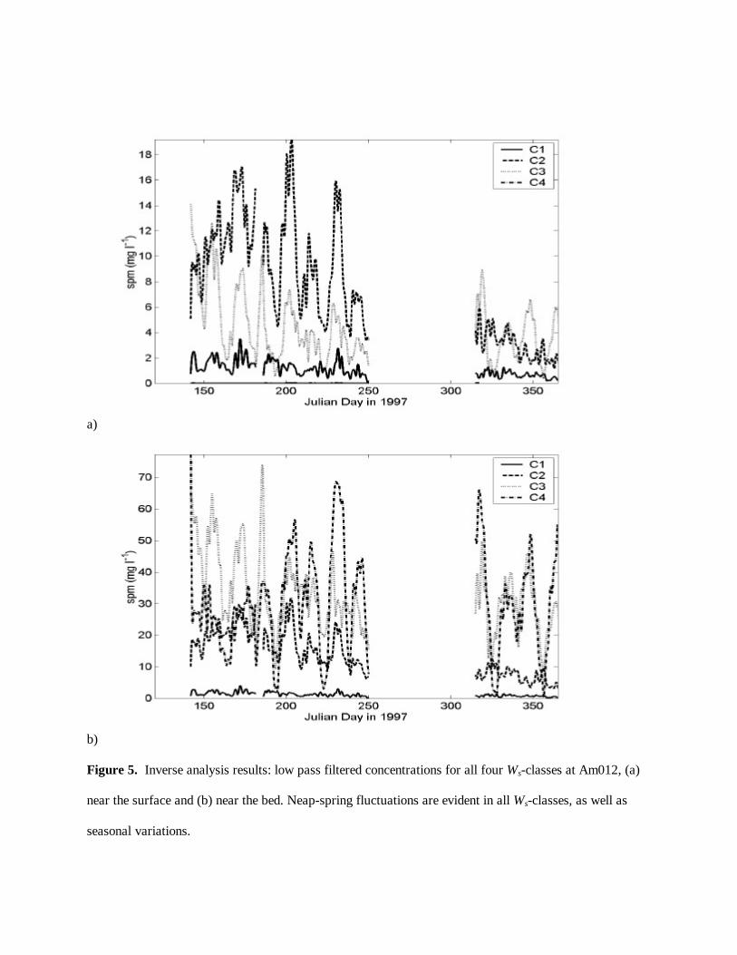
a)
b)
Figure 5. Inverse analysis results: low pass filtered concentrations for all four Ws-classes at Am012, (a)
near the surface and (b) near the bed. Neap-spring fluctuations are evident in all Ws-classes, as well as
seasonal variations.
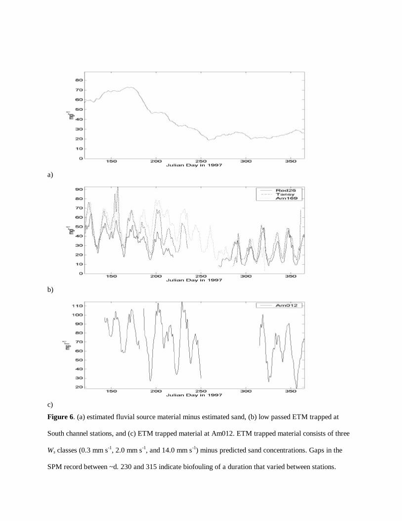
a)
b)
c)
Figure 6. (a) estimated fluvial source material minus estimated sand, (b) low passed ETM trapped at
South channel stations, and (c) ETM trapped material at Am012. ETM trapped material consists of three
Ws classes (0.3 mm s-1, 2.0 mm s-1, and 14.0 mm s-1) minus predicted sand concentrations. Gaps in the
SPM record between ~d. 230 and 315 indicate biofouling of a duration that varied between stations.
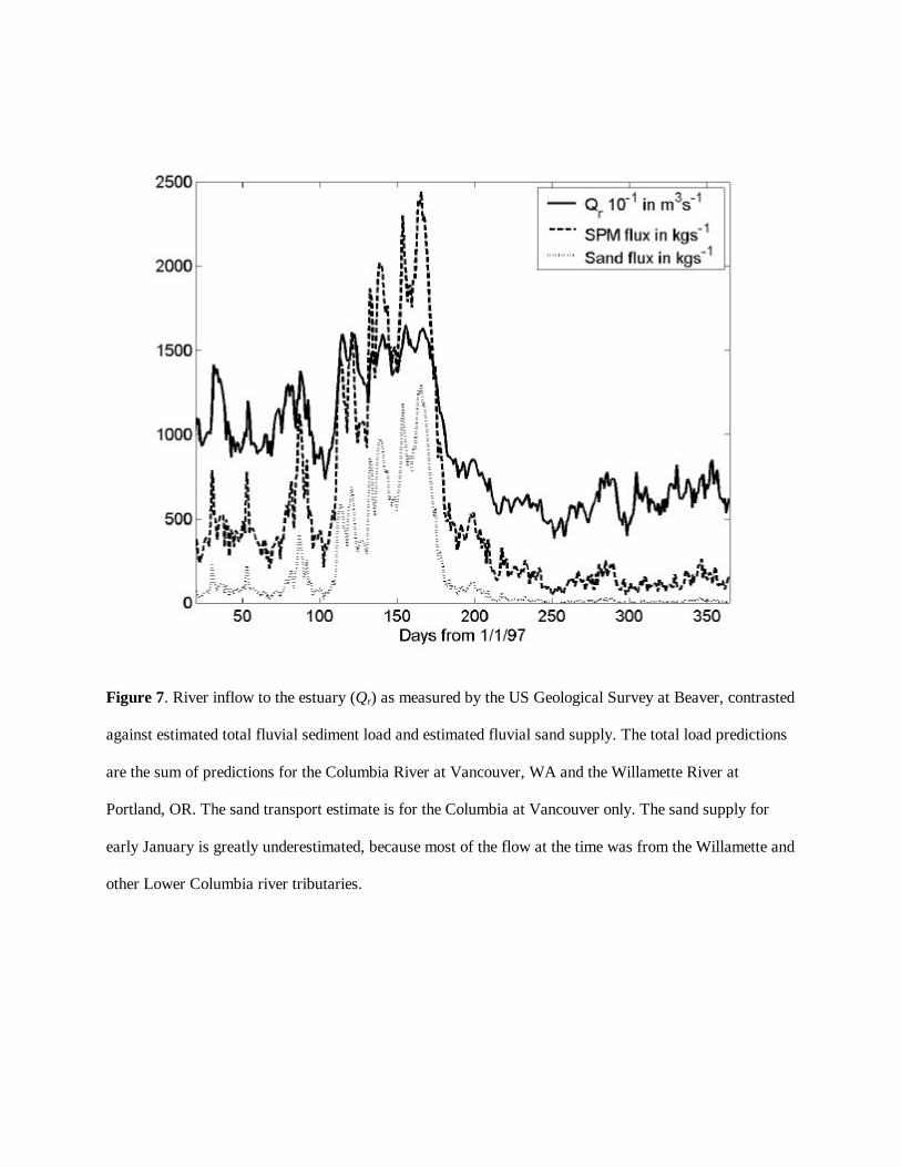
Figure 7. River inflow to the estuary (Qr) as measured by the US Geological Survey at Beaver, contrasted
against estimated total fluvial sediment load and estimated fluvial sand supply. The total load predictions
are the sum of predictions for the Columbia River at Vancouver, WA and the Willamette River at
Portland, OR. The sand transport estimate is for the Columbia at Vancouver only. The sand supply for
early January is greatly underestimated, because most of the flow at the time was from the Willamette and
other Lower Columbia river tributaries.
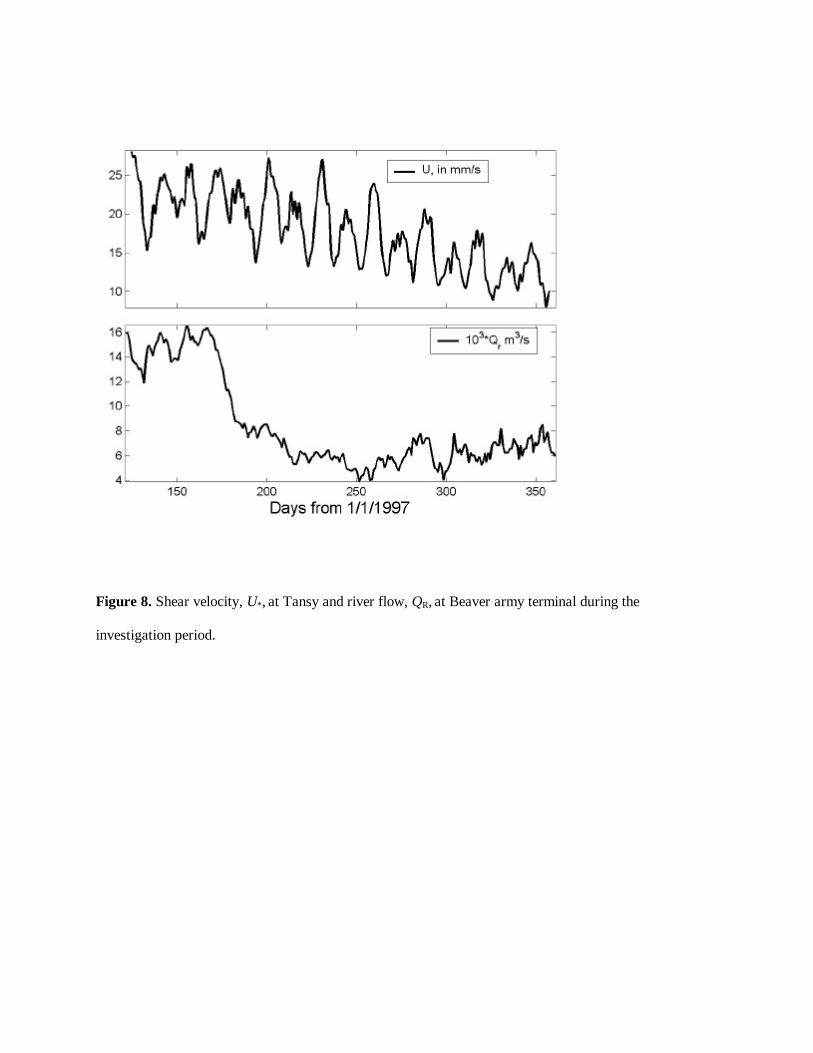
Figure 8. Shear velocity, U*, at Tansy and river flow, QR, at Beaver army terminal during the
investigation period.
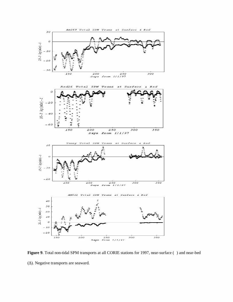
Figure 9. Total non-tidal SPM transports at all CORIE stations for 1997, near-surface (�) and near-bed
(∆). Negative transports are seaward.
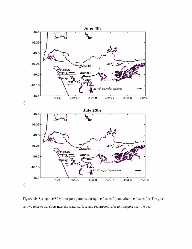
a)
b)
Figure 10. Spring tide SPM transport patterns during the freshet (a) and after the freshet (b). The green
arrows refer to transport near the water surface and red arrows refer to transport near the bed.
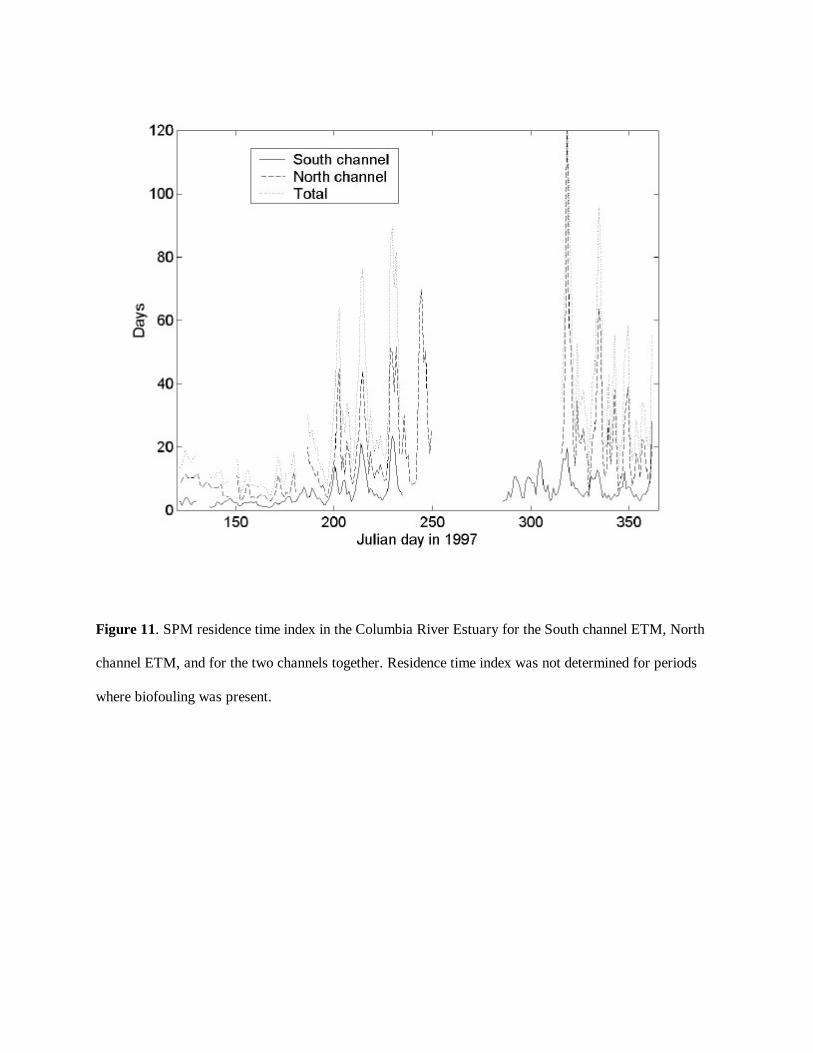
Figure 11. SPM residence time index in the Columbia River Estuary for the South channel ETM, North
channel ETM, and for the two channels together. Residence time index was not determined for periods
where biofouling was present.
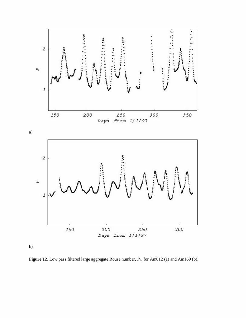
a)
b)
Figure 12. Low pass filtered large aggregate Rouse number, P4, for Am012 (a) and Am169 (b).
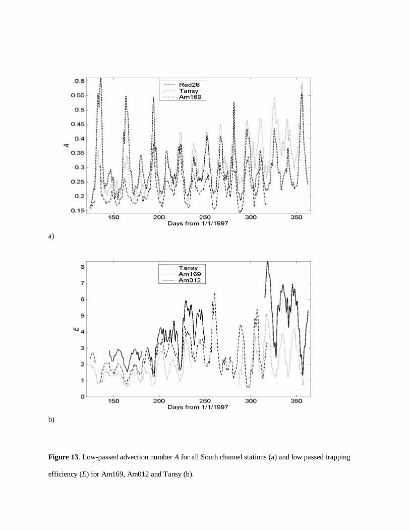
a)
b)
Figure 13. Low-passed advection number A for all South channel stations (a) and low passed trapping
efficiency (E) for Am169, Am012 and Tansy (b).
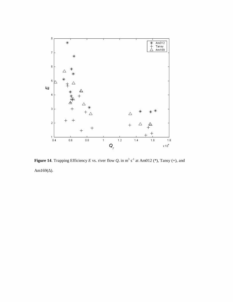
Figure 14. Trapping Efficiency E vs. river flow Qr in m3 s-1 at Am012 (*), Tansy (+), and
Am169(∆).