Embed Size (px)
Citation preview

Market SegmSelection f
(Revised V
Faculty & Research
entation and Product Technology or Remanufacturable Products
by
L. Debo B. Toktay
and L. Van Wassenhove
2003/81/TM
ersion of 2001/47/TM/CIMSO
Working Paper Series
Market Segmentation and Product TechnologySelection for Remanufacturable Products
Revised version of INSEAD WP 2001/47/TM/CIMSO 18
Laurens G. DeboGraduate School of Industrial Administration
Carnegie-Mellon UniversityPittsburgh, PA 15213, USA
L. Beril ToktayTechnology Management
INSEAD77305 Fontainebleau, France
Luk N. Van WassenhoveTechnology Management
INSEAD77305 Fontainebleau, France
September 2003
Abstract Remanufacturing is a production strategy whose goal is to recover the residual value
of used products. Used products can be remanufactured at a lower cost than the initial production
cost, but remanufactured products are valued less than new products by consumers. The choice
of production technology influences the value that can be recovered from a used product. In
this paper, we solve the joint pricing and production technology selection problem faced by a
manufacturer who considers introducing a remanufacturable product in a market that consists of
heterogeneous consumers. Our analysis discusses the market and technology drivers of product
remanufacturability and identifies some phenomena of managerial importance that are typical of a
remanufacturing environment.
1 Introduction and Literature Review
Remanufacturing is a production strategy whose goal is to recover the residual value of used prod-
ucts by reusing components that are still functioning well. Remanufactured products are obtained
by collecting used products and replacing worn-out components by new ones (Thierry et al. 1995).
The remanufacturing literature focuses mainly on logistics, production planning and inventory con-
trol (Fleischmann et al. 1997), but these considerations constitute only one facet of the managerial
issues surrounding remanufacturing. Consider the tire manufacturing and retreading industry, for
example. The casing (the inner structure of the tire) may be reusable even after the tread (the outer
layer) wears out. The remanufacturing activity consists of “retreading,” a process that replaces
the worn tread by a new one. By law, retreaded tires have to be marked on the side-wall (Com-
mission of The European Communities 2000), which allows consumers to distinguish between new
and retreaded tires. Typically, retreads are perceived to have lower quality than new tires (Prejean
1989). The retreadability of tires can be influenced by the manufacturer (BIPAVER 1998, Bozarth
2000a), via the choice of material and production technology, but increased retreadability requires
a higher production cost. Tire manufacturers face these issues in making production technology
and product pricing decisions.
Similar considerations are relevant in a variety of industries. Klausner et al. (1998) describe the
remanufacturing of electrical motors. Most electrical motors last longer than the product that they
power. Products containing remanufactured electrical motors can be sold to low-end consumers at
a discounted price. Whether a used motor can be remanufactured depends on the usage pattern,
but this is unobservable by the manufacturer. Integrating an Electronic Data Log (EDL) into the
motor at additional cost makes it easier to assess whether the motor is remanufacturable or not, and
may also facilitate the remanufacturing operation. The question is whether it is worth incurring
the extra cost of installing an EDL on new motors.
Xerox has invested in the remanufacturability of its copiers (Vietor 1993) and has been successful
in marketing its remanufactured product line. With the digitalization of the copier, Xerox faces
a new challenge: The cost of software upgrades required in remanufacturing the used copier may
be too high to be recovered given the low willingness-to-pay of consumers for the remanufactured
copier.
In this paper, we address the key managerial issues faced by a manufacturer who considers
producing a remanufacturable product, where consumers are heterogeneous in their willingness to
pay and where they value remanufactured products less than new products. The most fundamen-
tal question is whether producing a remanufacturable product is profitable. A remanufacturable
product is typically more costly to produce than a single-use product. The revenue potential of the
1
remanufactured product is questionable when it is valued less than the new product by consumers.
On the other hand, the remanufactured product is cheaper to manufacture and creates the oppor-
tunity to sell to the low-end consumers. In this context, the key questions facing the manufacturer
are the following: Does the opportunity to reach low-end consumers outweigh the high cost of
producing a remanufacturable product? What are the key drivers determining the profitability of
offering a product portfolio consisting of a new and a remanufactured product? How do the costs
and consumer perceptions impact the value proposition of remanufacturability?
The relative size of the low-end and high-end consumer populations differs across markets. An
important issue in this context is understanding the impact of the characteristics of the target
market: Does the decision to remanufacture depend on the consumer profiles? What pricing
strategy and production technology choice best fit the target market?
The combination of new and remanufactured products creates a unique product portfolio in the
sense that the remanufactured product exists only due to previous sales of the new product. Thus,
a decrease in demand for new products results in a decrease in the availability of remanufactured
products. It is useful to understand the implications of this dependence for planning and marketing
purposes. For example, how does this dependence influence optimal sales volume dynamics in
the introduction phase of the portfolio? How does the remanufacturing cost impact the desired
production volume and mix? From a marketing perspective, an important managerial question is
how to position the new product: Is it valued for the immediate margin it creates or for the future
value stream that it has the potential to generate? What should be the pricing policy that reflects
the role of the new product?
The literature on remanufacturing has focused primarily on operational issues that arise in
inventory management and production control as a result of the return flows of used products.
These issues include disassembly (Guide and Srivastava 1998), MRP for product recovery (Inder-
furth 1998), scheduling and shop floor control (Guide et al. 1997) and inventory management (van
der Laan et al. 1999, Toktay et al. 2000, Inderfurth 2002). Fleischmann (2000) considers reverse
logistics network design. In these papers, price, demand rate, and remanufacturability level are
assumed to be exogenous, and consumers do not differentiate between new and remanufactured
products. The focus is on determining the cost-minimizing operating policy or system design for a
given remanufacturability level and price. Our paper complements this literature by determining
the remanufacturability level and the optimal prices using a market model that reflects how reman-
ufactured products are perceived by consumers. Other researchers modelling market-related issues
in remanufacturing are Savaskan et al. (1999) who determine the optimal collection channel con-
figuration of a monopolist manufacturer, and Groenevelt and Majumder (2001a,b) who investigate
the impact of competition between a manufacturer who also performs remanufacturing activities,
2
and a local remanufacturer.
The literature on market segmentation (Mussa and Rosen 1978, Moorthy 1984) studies the opti-
mal pricing of independent products that are differentiated by quality in a market of heterogeneous
consumers whose valuations of quality vary. In a remanufacturing setting, there is a dependence
between the two products: The supply of used products that can be remanufactured depends on
past sales volumes of new products and the level of remanufacturability. Ferrer (2000) solves the
market segmentation problem for a fixed remanufacturability level. He finds that remanufacturing
is not viable if the resulting cost savings are not high enough to price the remanufactured product
above its marginal cost. We consider the simultaneous determination of product prices and the
production technology for a general consumer profile. One of our results complements Ferrer’s
findings by determining under which circumstances his pure cost savings analysis is sufficient to
determine the viability of remanufacturing.
The remainder of this paper is structured as follows: In §2, we introduce the basic model in
which the monopolist determines the remanufacturability level of the new product and segments
the market between new and remanufactured products. In §3, we solve and interpret the optimal
solution to the manufacturer’s problem to answer the questions raised in the introduction. §4extends our monopoly model to the case where remanufacturers compete on the remanufactured
product market. In §5, we discuss the implications of our results for the integrated management
of product lines with new and remanufactured products. We conclude with directions for future
research.
2 The Model
We introduce our assumptions concerning the production technology, the cost structure, the con-
sumer preferences, the industry structure, and the decision-making framework in §2.1 and formulate
the manufacturer’s optimization problem in §2.2.
2.1 Assumptions
Production Technology Choice. Motivated by the examples of §1, we assume that the man-
ufacturer controls the level of remanufacturability through the choice of production technology.
We model the remanufacturability level, denoted by q, as the fraction of products that can be
remanufactured after one period of use. The manufacturer can choose any remanufacturability
level q ∈ [0, 1]. If the remanufacturability level is set to zero, this is a “single-use” product and
cannot be remanufactured. Used remanufacturable products require a remanufacturing operation
3
before being sold as remanufactured products. We assume that a remanufacturable product can
be remanufactured at most once.
Cost Structure. The technology choice impacts both up-front costs independent of subsequent
production volume such as R&D expenditure, as well as costs that are a function of the production
volume. We model the impact of technology choice on the former costs by means of a fixed cost k (q)
incurred before production starts. We assume that k (q) is a convex increasing function of q with
k (0) = 0. We model the dependence of the new-product unit manufacturing cost and used-product
unit remanufacturing cost on the technology choice by cn (q) and cr (q), respectively. We assume
that cn (q) is a convex increasing function of q and that cr (q) is a non-increasing function of q: A
higher level of remanufacturability requires a higher new product unit manufacturing cost (due to
the use of better materials, more precise production processes, addition of a data logger, etc.), and
at the same time, can result in a lower unit remanufacturing cost (due to easier disassembly, less
testing etc.).
Since our goal is to model the interaction between production technology and pricing at a strategic
level, we do not attempt to model the details of the production environment such as raw material
or capacity constraints, economies of scale, production lead times, etc.
Consumer preferences. Consumers typically differ in their willingness-to-pay. For this reason,
we associate with each consumer its willingness-to-pay for a new product, θ, also called its ‘type’.
We refer to consumers with a low (high) willingness-to-pay for new products as ‘low-end’ (‘high-
end’) consumers. We assume that θ is distributed on [0, 1] according to a function F, where F (θ)
denotes the volume of consumers with willingness-to-pay in [0, θ] and is a strictly increasing and
continuous function with F (0) = 0 and F (1) = 1. Markets differ in the relative concentration
of consumers with different levels of willingness-to-pay. Introducing a general structure for F
allows us to capture this variety. In particular, we consider a class Fκ of distributions of the form
F (θ) = 1 − (1 − θ)κ, where κ ∈ (0,∞). The uniform distribution frequently used in the market
segmentation literature is a special case of this distribution obtained by setting κ = 1.
Typically, remanufactured products are valued less than new products by consumers. For
example, Xerox studies showed that the presence of used components in a remanufactured product
decreased the consumer’s willingness-to-pay for this product (Vietor). Furthermore, retreaded tires
are typically bought by budget-conscious consumers (Alford 2001). The retread industry has also
been plagued with image problems (Prejean). To model this, we assume that the willingness-to-
pay of consumer type θ for a remanufactured product is (1 − δ)θ. We refer to δ as the “perceived
depreciation” of the remanufactured product. This model implies that low-valuation consumers are
less sensitive to perceived depreciation: d(1−δ)θdδ = −θ, that is, the loss in utility due to a change
in the perceived depreciation is less for low consumer types. We refer to (F, δ) as the ‘consumer
4
profile.’
Let pN and pR denote the prices of new and remanufactured products, respectively. We model
the net utility that a consumer of type θ derives from buying a new product, a remanufactured
product, and no product, by θ−pN , (1−δ)θ−pR, and 0, respectively. In a given period, consumers
choose which product to buy based on the utility that they derive in that period from this purchase.
Industry Structure. Our main analysis and discussion (§3) is for an industry in which the manu-
facturer holds a monopoly in the markets for new and remanufactured products. This assumption
is reasonable if the manufacturer has a proprietary remanufacturing technology (e.g. MRT retread
technology developed by Michelin) that would limit the formation of a market for used reman-
ufacturable products, and the supply of used but remanufacturable products is controlled by the
manufacturer (e.g., Michelin’s retread company, Pneu Laurent, operates a fleet of over two hundred
vehicles collecting used Michelin tires from dealers). Nevertheless, independent competing reman-
ufacturers abound in this industry, as in other industries (Groenevelt and Majumder 2001a,b). To
capture the impact of competition in the remanufactured product market on the remanufactura-
bility level chosen by the manufacturer, we consider an industry in which the manufacturer holds
a monopoly in the market for new products, and independent remanufacturers compete on the
remanufactured product market. This variant is analyzed in §4.
The Decision-Making Framework. The manufacturer’s goal is to maximize the net present
value of introducing a remanufacturable product, calculated over the life-cycle of this product, by
determining the level of remanufacturability and a sequence of prices for the new and remanufac-
tured products.
To model this, we develop a discrete-time, infinite-horizon, discounted profit optimization prob-
lem. Each period corresponds to a period of use of the product by a consumer, after which the
product needs to be remanufactured for further use. This period may range from several weeks
(e.g. single-use cameras) to several months (e.g. tires). Let β denote the discount factor over this
time period. Thus, the longer the time on the market, the lower the discount factor should be.
We assume that the level of remanufacturability is determined at time 0 since it is the initial
technology choice that determines this value for all subsequent periods. Product prices are allowed
to be time-dependent. Recall that the supply of used products that can be remanufactured in each
period is constrained by the historical sales of new products and the level of remanufacturability.
Starting without a supply of used products induces a transient period during which this supply
is built up. We allow the manufacturer to carry inventory of used remanufacturable products. In
order to keep the focus on the technology selection and market segmentation issues, we do not
consider associated holding costs.
5
The infinite-horizon assumption is particularly appropriate when the period of use of a product
is short relative to the total life-cycle of the product on the market, as is the case with tires and
electrical motors, for example. Moreover, the infinite horizon analysis provides some insight into
problems with a finite, but sufficiently long, horizon. Finally, the infinite-horizon framework lends
itself to an approximate analysis of the optimal technology choice based on the stationary solution
and allows us to derive a number of comparative statics results.
2.2 Formulation of the Monopolist’s Optimization Problem
The Single-Period Profit.
Recall that pN and pR denote the prices of new and remanufactured products, respectively, and
define p.= (pN , pR), where p ∈ S .
= (pN , pR) ∈ R2+ : 0 ≤ pN ≤ 1, 0 ≤ pR ≤ (1 − δ) pN. Then
ΩN (p).= θ ∈ [0, 1] : θ − pN ≥ (1 − δ) θ − pR is the set of consumer types who purchase a new
product. ΩR (p) is defined analogously as the set of consumer types who purchase a remanufactured
product.
Let n and r denote the volume of consumers who purchase new and remanufactured products,
respectively, and define ν.= (n, r). Then n =
∫ΩN (p) dF (θ) and r =
∫ΩR(p) dF (θ). By construction,
ν ∈ D .=(n, r) ∈ R
2+ : n + r ≤ 1
. Since F is strictly increasing, the mapping p → ν(p) is one-
to-one. Therefore, the inverse mapping ν ∈ D → p (ν) ∈ S is well defined. We can now define
R (ν).= npN (ν)+rpR (ν), the revenue of the monopolist who prices so as to create demand ν. Some
properties of the revenue function are developed in §8.1. Finally, let π (ν, q).= R (ν) − cn (q) n −
cr (q) r; this is the profit obtained in a generic period under the decision (ν, q).
The Infinite-Horizon Optimization Problem.
Let st.= (sN,t, sR,t) be the sales of new and remanufactured products in period t. Let It denote
the supply of used products that can be remanufactured that remain in stock at the beginning
of period t from returns in previous periods. Then, I0 = 0 and sR,0 = 0 since no used products
exist initially and It =∑t
k=1 qsN,t−k − sR,t−k. If the price in period t, pt, is chosen such that the
resulting demand for remanufactured products is greater than the available inventory (rt > It), the
manufacturer can only sell sR,t = min (rt, It) = It. In this case, the manufacturer can increase both
pR,t and pN,t in such a way that the demand for remanufactured products decreases to It and the
demand for new products remains the same. Since the sales volumes remain identical while both
prices increase, a higher profit can be realized in this manner. Therefore, it will never be optimal
to price such that rt > It; at optimality, rt ≤ It and sR,t = rt. In addition, as a result of our
assumptions on production capacity, production lead times and raw material supply, any volume of
new products can be satisfied, that is, sN,t = nt. Thus, we can formulate our problem in terms of
6
demand volumes and define the feasible region such that the demand for remanufacturable products
in each period is less than or equal to the available supply of used remanufacturable products. We
define an implementable path P starting with initial remanufacturable product inventory I (denoted
by P ∈ I(I)) as P .= νt, t ≥ 0|νt ∈ D, I0 = I, It = It−1 + qnt−1 − rt−1 ∀t ≥ 1, and rt ≤ It ∀t ≥ 0.
The analysis in the remainder of this paper will use nt and rt as decision variables.
Let Vβ(I; q) denote the optimal β-discounted infinite-horizon profit of the manufacturer for a
given remanufacturability level q under the initial condition I0 = I, i.e., Vβ (I; q).= max
P∈I(I)
∑∞t=0 βtπ (νt, q).
In this paper we analyze this problem for I0 = 0. We define Vβ(q).= Vβ(0; q), that is,
Vβ (q).= max
P∈I(0)
∞∑
t=0
βtπ (νt, q) . (1)
The optimal solution to this problem is the path of new and remanufactured demands ν∗t , to which
corresponds a unique optimal price path p∗t .
The technology selection problem of a manufacturer with a monopoly position in both markets
for new and remanufactured products is then
maxq∈[0,1]
Vβ (q) − k (q) . (2)
3 Analysis
We characterize the optimal solution of the monopolist’s optimization problem in §3.1. In §3.2,
we derive a sufficient condition under which it is optimal for the manufacturer to invest in the
remanufacturability of its product. §3.3 discusses the evolution of demand volumes during the
introduction phase of a remanufacturable product. § 3.4 focuses on the stationary solution to
explore the characteristics of the optimal portfolio. In particular, we investigate the dependence
of the optimal remanufacturability level on the consumer profile (§3.4.1), we characterize new and
remanufactured product margins (§ 3.4.2) and we establish properties of the demand mix as a
function of the remanufacturing cost (§3.4.3).
3.1 A Characterization of the Optimal Solution
Let c (q).= cn (q) + βqcr (q), v (q)
.= ∂R(0,0)
∂n + qβ ∂R(0,0)∂r , ν
.= (n, r)
.= arg max
ν∈Dπ (ν, q) and
nsu.= arg max
0≤n≤1π (n, 0, 0). Here, c (q) and v (q) are the marginal present cost incurred and revenue
realized, respectively, when manufacturing and selling the new product now, and remanufacturing
the resulting used but remanufacturable products and selling them one period later; ν is the opti-
mal single-period demand (sales) volumes unconstrained by availability of used remanufacturable
7
products, and nsu is the optimal demand (sales) volume of single-use products (products which
have remanufacturability level q = 0). If ν ∈ int (D), then ∂R(ν)∂n = cn (q) and ∂R(ν)
∂r = cr (q). If
0 < nsu < 1, then ∂R(nsu,0)∂n = cn (0).
Some assumptions that are used in the following analysis, but were not discussed in §2 are listed
in § 8.2. We do not repeat any assumptions in the statement of each result; it is implicit that they
hold throughout the analysis.
Lemma 1 Let q ∈ [0, 1] and I0 = I. Then (i) Vβ (I; q) is concave nondecreasing in I; (ii) There
exists a unique optimal path ν∗t , t ≥ 0; call it P∗
q (I0).
Let n∗(I) and r∗(I) denote the unique maximizers of the right-hand side in the Bellman Equation
v (I; q) = maxν∈D,r≤I
π (ν, q) + βv (I + qn − r; q) . (3)
Define the policy function g such that g(I).= I + qn∗(I) − r∗(I). The optimal path starting with
initial condition I0 = 0, denoted by P∗q , is found by applying g recursively to It starting with I0 = 0.
Then n∗t = n∗(It), r∗t = r∗(It) and It+1 = g(It) ∀t. We characterize properties of the optimal path
and/or of Vβ(q) as follows: Lemma 2 identifies a necessary and sufficient condition for Vβ(q) > 0.
Subject to this condition, Lemma 3 characterizes the optimal path and V ′β(q) when qn ≥ r and
Proposition 1 builds on Lemmas 6 and 7 (in §8.3) to characterize the optimal path and to derive
V ′β(q) when qn < r. In particular, Lemma 6 derives the shape of the policy function g and Lemma
7 shows that It → I∞ and ν∗t → ν∞, the stationary solution.
Lemma 2 Vβ (q) > 0 if and only if c (q) < v (q).
Lemma 3 Let q > 0. If c(q) < v (q) and qn ≥ r, then P∗q = (ns(q), 0) , (n, r) , (n, r) , (n, r) ...,
where ns.= arg max
0≤n≤1π (n, 0, q). In addition, V ′
β(q) < 0.
Lemmas 2 and 3 imply that q∗ ∈ Q.= q ∈ [0, 1]|c(q) < v (q) and qn < r. For the remainder of
the paper, we work with q ∈ Q.
Proposition 1 Let P∗q = ν∗
t , t ≥ 0 ∈ I(0) be the optimal path found when solving (1) for a fixed
q. Then, it satisfies∂R (νt)
∂n+ βq
∂R (νt+1)
∂r= c (q) ∀t. (4)
In addition,
V ′β (q) =
∞∑
t=0
βt
(β
(∂R(ν∗
t+1
)
∂r− cr (q)
)n∗
t − c′n (q) n∗t − c′r (q) r∗t
). (5)
8
Equations (4) and (5) have the following economic interpretation: Increasing the volume of new
products during a single period results in an immediate increase in revenues from new products,∂R(ν∗
t )∂n , and an increase in revenues from remanufactured products in the next period on a fraction q
of new products∂R(ν∗
t+1)∂r . Equation (4) equates the marginal increase in revenues over two periods
with the marginal increase in cost over two periods (c (q)). Equation (5) calculates the effect of
increasing q by dq. This change has an effect over all periods: An increase in unit manufacturing
and remanufacturing costs in period t by (c′n (q) n∗t + c′r (q) r∗t ) dq, but also an increase in revenues
in the next period, due to an increase drt+1 = n∗t dq in available remanufacturable units which
generates an additional profit
(∂R(ν∗
t+1)∂r − cr (q)
)n∗
t dq.
We build on Equations (4) and (5) to derive the results in the next subsections.
3.2 Whether to Produce a Remanufacturable Product
In this subsection, we discuss the conditions under which the solution q∗ to (2) is strictly positive,
that is, the manufacturer invests in the remanufacturability of his product. Let us define ∆.=
V ′β (0) − k′(0). We call ∆ the ‘remanufacturing potential’: If ∆ is positive, then, it is profitable to
produce a remanufacturable product.
Proposition 2 It is optimal to produce a remanufacturable product (i.e. q∗ > 0) if the following
condition is satisfied:
∆ =1
1 − β
(β (1 − δ) cn (0) − cr (0) − c′n (0)
)nsu − k′ (0) > 0. (6)
We will now discuss the impact of all technology and market related parameters on the reman-
ufacturing potential.
3.2.1 Factors Directly Influencing the Remanufacturing Potential
From (6), we observe that the remanufacturing potential ∆ increases as the product becomes
cheaper to remanufacture (cr (0) decreases), or the marginal increase in the unit cost c′n (0) de-
creases, or the marginal increase in the fixed cost k′ (0) decreases. These factors all relate to
incremental costs associated with moving from a single-use product to a remanufacturable prod-
uct. Note also that ∆ increases in the discount factor, β, which is influenced by the length of time
the new product stays on the market before it returns to the manufacturer (the length of one period
in our model). Furthermore, ∆ increases as δ, the perceived depreciation factor, decreases. These
parameters are direct drivers of the remanufacturing potential.
9
3.2.2 Factors Indirectly Influencing the Remanufacturing Potential
The manufacturing cost cn(0) has a direct positive impact on ∆. In addition, both cn(0) and the
consumer profile (F, δ) play a role in determining ∆ via the term nsu. In order to gain insight into the
role of the consumer profile, we focus on the class Fκ of distributions of the form F (θ) = 1−(1 − θ)κ,
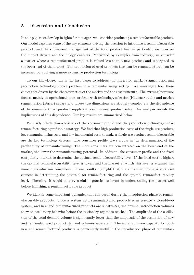
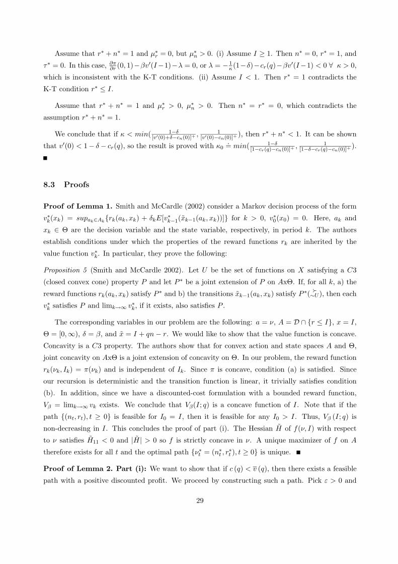
where κ ∈ (0,∞). Figure 1 plots the density f(θ) for four different values of κ. Observe that as κ
increases, the mass of consumers shifts from high-valuation consumers to low-valuation consumers.
0 0.1 0.2 0.3 0.4 0.5 0.6 0.7 0.8 0.9 10
0.5
1
1.5
2
2.5
3
3.5
4
θ
κ=5
κ=1
κ=0.5
κ=0.1
f(θ)
Figure 1: f (θ) = κ (1 − θ)κ−1 for κ = 0.1, 0.5, 1 and 5.
Proposition 3 Let F ∈ Fκ. If β (1 − δ) cn (0) − cr (0) > c′n (0), then d∆dκ < 0 and d∆
dcn(0) ≶ 0.
As expected, when the mass of consumers shifts towards the lower end of the spectrum (κ
increases), the optimal sales volume of single use products, nsu, decreases. Therefore, the remanu-
facturing potential decreases. Note that the distribution of consumer types F (θ) impacts the sign
of the remanufacturing potential only when k′ (0) > 0, and not when k′ (0) = 0.
It is interesting to note that increasing the cost of single-use products impacts the remanufac-
turing potential in two opposing ways. On one hand, through the term (1 − δ)cn(0), the remanu-
facturing potential increases as the unit production cost increases. The intuition is the following:
When q = 0, the optimal path is n∗t = nsu ∀t. It follows that
∂R(ν∗t )
∂r = ∂R(nsu,0)∂r in (5) for q = 0.
10
Parameter, Interpretation Impact on
increasing potential
cr (0) remanufacturing cost negative
k′ (0) increase in fixed cost negative
β discount factor/sojourn time on market positive
δ perceived depreciation negative
c′n (0) increase in unit new product costs negative
cn (0) single use production cost pos./neg.
κ consumer profile negative
Table 1: Determinants of profitability of remanufacturing
For our consumer preference model, it can be shown that ∂R(n,0)∂r = (1 − δ) ∂R(n,0)
∂n for any n ∈ [0, 1].
By the definition of nsu, ∂R(nsu,0)∂n = cn(0), and we obtain the term ∂R(nsu,0)
∂r = (1 − δ) cn (0) in ∆.
It may seem counter-intuitive that the marginal cost cn (0) contributes to the marginal profit (∆).
However, this makes sense in a remanufacturing context since remanufacturing is a strategy that
exploits the reduction in production cost. Therefore, all else being equal, a higher production cost
to start with (without remanufacturing), makes remanufacturing more attractive.
On the other hand, the sales of single-use products, nsu, decrease as cn (0) increases. Therefore,
in the presence of a fixed cost, it may be that expensive single-use products are not profitable
to remanufacture, because the sales of single-use products is too limited to generate a profitable
market for remanufactured products. On the other hand, when k′ (0) = 0, sufficiently expensive
single-use products will have a positive remanufacturing potential.
3.2.3 Summary of Factors Influencing the Remanufacturing Potential.
We summarize the direct and indirect drivers of profitability of remanufacturing in Table 1. A nec-
essary, but not sufficient, condition for a positive remanufacturing potential can be found between
in (6): If (1 − δ) cn (0) − cr (0) < 0, then the lowest consumer type to whom a new product can
be sold without a loss (θ = cn (0)) has a willingness-to-pay (1 − δ) cn (0) for the remanufactured
product that is lower than the production cost of the remanufactured product (cr (0)) and reman-
ufacturing is not viable. Therefore, the condition (1 − δ) cn (0) − cr (0) > 0 is necessary (but not
sufficient) to assure a positive remanufacturing potential. In the emerging operations literature on
remanufacturing, pure production cost savings cn(0)− cr (0) are often assumed to drive remanufac-
turing activities (Klausner et al., Savaskan et al., Ferrer). Condition (6) generalizes this construct
significantly to take into account the characteristics of the consumer profile, discounting, and the
11
incremental cost of providing remanufacturability.
3.3 Dynamics of Introducing Remanufacturable Products
In this subsection, we investigate the dynamics of optimal sales volumes during the transient period
for a given remanufacturability level q by linearizing (4) around the stationary solution ν∞.
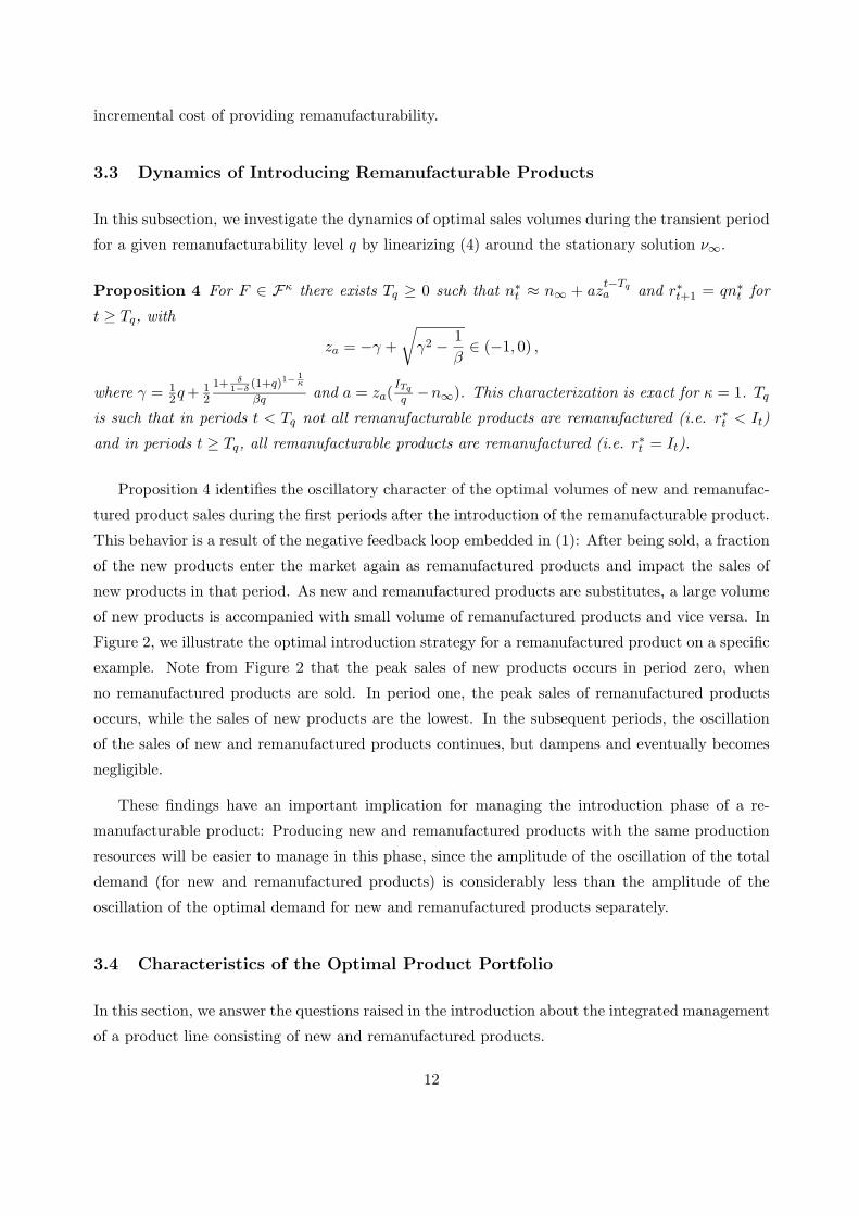
Proposition 4 For F ∈ Fκ there exists Tq ≥ 0 such that n∗t ≈ n∞ + az
t−Tqa and r∗t+1 = qn∗
t for
t ≥ Tq, with
za = −γ +
√γ2 − 1
β∈ (−1, 0) ,
where γ = 12q + 1
2
1+ δ1−δ
(1+q)1−1κ
βq and a = za(ITq
q −n∞). This characterization is exact for κ = 1. Tq
is such that in periods t < Tq not all remanufacturable products are remanufactured (i.e. r∗t < It)
and in periods t ≥ Tq, all remanufacturable products are remanufactured (i.e. r∗t = It).
Proposition 4 identifies the oscillatory character of the optimal volumes of new and remanufac-
tured product sales during the first periods after the introduction of the remanufacturable product.
This behavior is a result of the negative feedback loop embedded in (1): After being sold, a fraction
of the new products enter the market again as remanufactured products and impact the sales of
new products in that period. As new and remanufactured products are substitutes, a large volume
of new products is accompanied with small volume of remanufactured products and vice versa. In
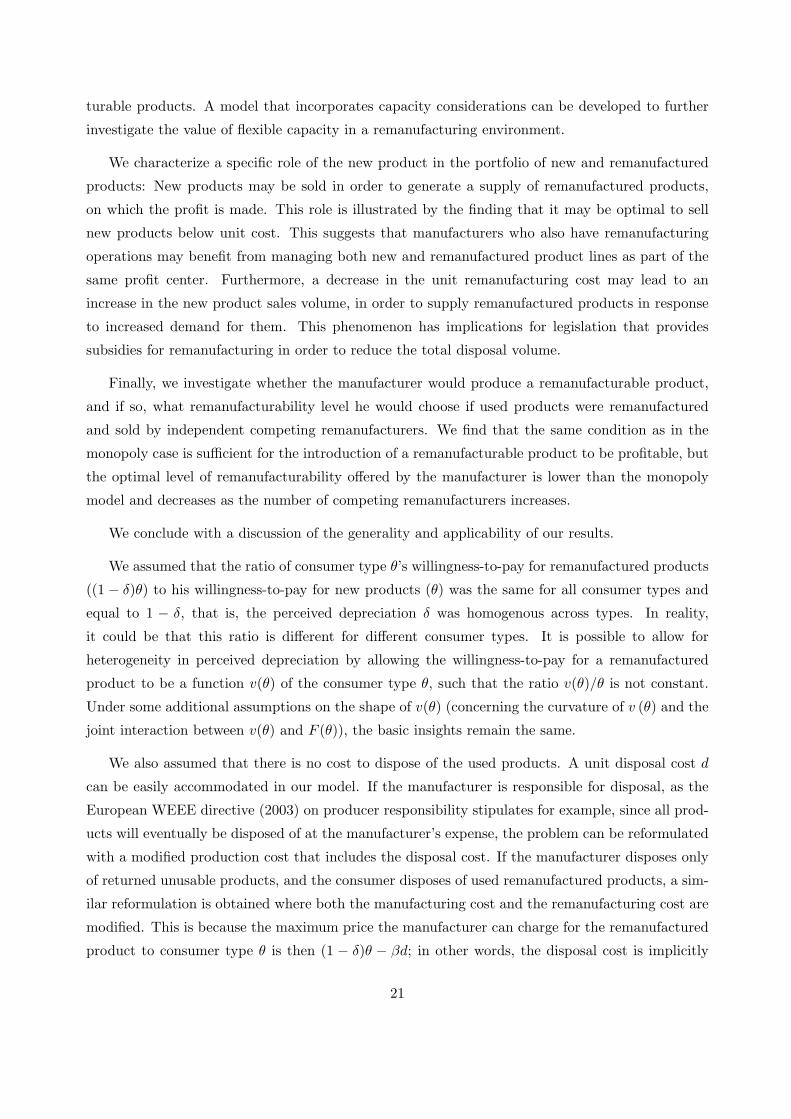
Figure 2, we illustrate the optimal introduction strategy for a remanufactured product on a specific
example. Note from Figure 2 that the peak sales of new products occurs in period zero, when
no remanufactured products are sold. In period one, the peak sales of remanufactured products
occurs, while the sales of new products are the lowest. In the subsequent periods, the oscillation
of the sales of new and remanufactured products continues, but dampens and eventually becomes
negligible.
These findings have an important implication for managing the introduction phase of a re-
manufacturable product: Producing new and remanufactured products with the same production
resources will be easier to manage in this phase, since the amplitude of the oscillation of the total
demand (for new and remanufactured products) is considerably less than the amplitude of the
oscillation of the optimal demand for new and remanufactured products separately.
3.4 Characteristics of the Optimal Product Portfolio
In this section, we answer the questions raised in the introduction about the integrated management
of a product line consisting of new and remanufactured products.
12
0
0.05
0.1
0.15
0.2
0.25
0.3
0.35
0 1 2 3 4 5 6 7 8 9 10 11 12 13 14 15 16 17 18 19
n
r
n+r
cn(q)=0.25-0.01ln(1-q), cr(q)=0.05
d=0.65, f =0.1, m=2
q=0.850426Tq=0
Figure 2: Dynamics of optimal sales volumes during the introduction of a remanufacturable product.
3.4.1 Fitting the Level of Remanufacturability to the Consumer Profile
In §3.2, we showed how the remanufacturing potential (which determines whether to invest in
remanufacturability) depends on the production costs and consumer profile F ∈ Fκ. In this
subsection, we wish explore how the optimal level of remanufacturability changes as a function of
the consumer profile, that is, we wish to characterize q∗ as a function of κ. Let q∗κ be the solution
of (2) parametrized by κ. An asymptotic analysis as β → 1− yields a characterization of q∗κ for
β ≈ 1.
Proposition 5 If F ∈ Fκ and β ≈ 1, then for a consumer profile with a higher concentration on
the lower end of the market (κa > κb), the optimal level of remanufacturability is higher: q∗κa> q∗κb
.
When there is a larger mass of low-end consumers (κ large), there is a higher volume of potential
buyers to be captured by offering a remanufactured product. A bigger supply of remanufactured
products can be generated by building a higher level of remanufacturability into the new product.
This would of course increase the fixed cost k(q), but when the discount factor is very high, the
initial fixed cost is inconsequential. Therefore, q∗κ increases monotonically in κ. In numerical
experiments, we observe that as κ increases, the optimal prices of both new and remanufactured
products decrease at an increasing rate. Combined with the fact that cn(q) increases in q, we see
that the optimal new product margin erodes rapidly in κ.
13
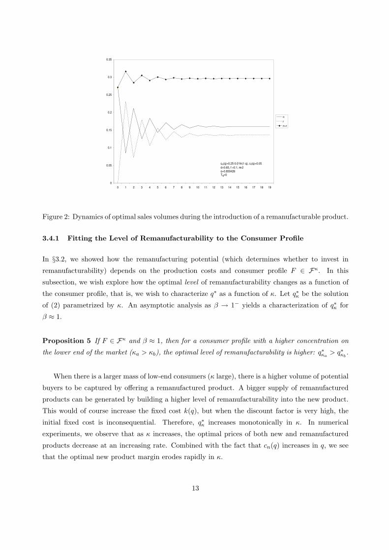
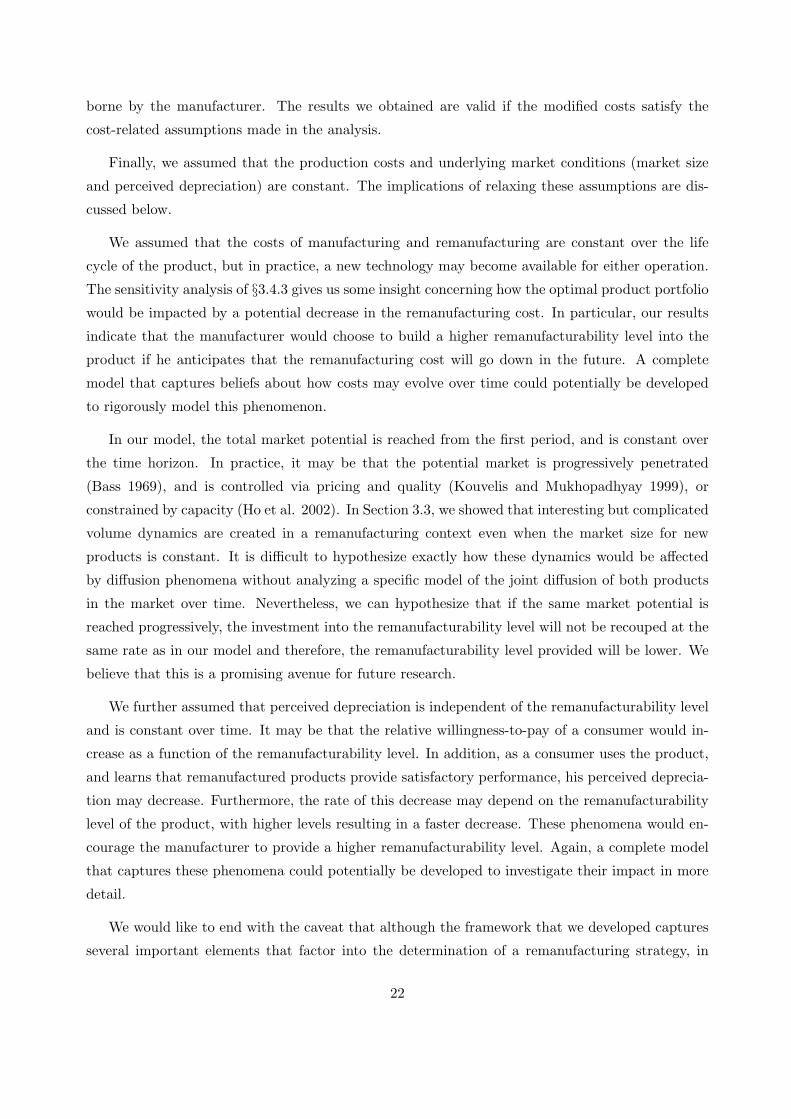
At lower discount factors, k(q) becomes consequential. To explore the impact of k(q), we
approximate the solution to (1) by linearizing (4) around ν∞ and find a closed-form expression
approximating V ′β (q). Let qκ denote the approximately optimal remanufacturability level obtained
using this expression. Figure 3 plots qκ for β = 0.7 and for different levels of fixed costs of the
form k(q) = kq. Recall from Proposition 2 that the remanufacturing potential decreases in κ and
k′(0), becoming negative after a threshold value of either factor. This is observed in Figure 3: For
each κ, there is a threshold value of k beyond which q∗ = 0; and for each fixed cost level, there is
a threshold value of κ beyond which q∗ = 0.
0
0.2
0.4
0.6
0.8
1
q
1 2 3 4 5
=0
=0.025
=0.050
=0.075
κ
~
k
k
k
k
Figure 3: qκ for k = 0, 0.025, 0.050 and 0.075 where k(q) = kq, for β = 0.7, cn (q) = 0.25 −0.05 ln (1 − q), cr = 0, and δ = 0.2.
Without a fixed cost (k = 0), we observe that qκ monotonically increases as a function of κ as
Proposition 5 leads us to expect. For k > 0, qκ first increases and then decreases in κ. This can be
explained as follows: As κ increases, reaching the low-end consumers by building a higher level of
remanufacturability becomes more attractive, so the optimal remanufacturability level increases.
However, since the fixed cost also increases in the remanufacturability level, there is a point beyond
which the fixed cost dominates and the optimal remanufacturability level starts to decrease in κ.
We can thus conclude that the optimal remanufacturability level is the highest for medium levels
of market heterogeneity. For markets with high concentrations of customers either on the high end,
or, on the low end, the optimal remanufacturability level is low. This result highlights that building
a high remanufacturability product is particularly suitable when catering to a diverse market.
14
3.4.2 The Role of the New Product
Due to the interdependence of new and remanufactured products, a decrease in demand for new
products results in a decrease in the availability of remanufactured products. We investigate the
implications of this dependence on pricing strategy. Let p∗∞ be the price vector that corresponds
to the optimal stationary demand volumes.
Proposition 6 Let F ∈ Fκ and β ≈ 1. There exists a consumer profile for which p∗N,∞ < cn(q∗).
Remanufactured product margins are always non-negative.
Proposition 6 reveals the dual role of new products: They have the potential of generating
profits in their own right. At the same time, they generate a volume of used products that are
sold at a profit after being remanufactured. In fact, the manufacturer may choose to produce some
new products only for the future value that they generate through their sale as remanufactured
products, although he sells them at a loss. This occurs in markets characterized by a large enough
concentration of low-valuation consumers: To tap into the low-valuation market, the manufacturer
needs to generate a high volume of remanufactured products, sometimes sacrificing margins on the
new product to do so. This effect is enhanced when the cost of manufacturing is high because
pricing above cost significantly limits the demand for new products in this case.
For a product whose value increases and/or whose cost decreases over time, Dhebar and Oren
(1985), Padmanabhan and Bass (1993), and Whang (1995) investigate the evolution of profit mar-
gins in a variety of contexts. They show that setting thin or negative margins initially may be
optimal; the low-value product is the “loss leader.” In contrast, in a remanufacturing context, the
loss leader is the high value product.
It is interesting to note that most manufacturer/remanufacturers manage the manufacturing
and remanufacturing operations separately. In particular, these operations are typically part of
separate profit centers. Our analysis reveals that this practice of focusing on the profits obtained
from new and remanufactured products separately can be counterproductive, and that considering
the total product line as part of the same profit center may lead to higher profitability for the firm.
3.4.3 The Impact of the Remanufacturing Cost
We explore the sensitivity of the optimal remanufacturability level and sales volumes to the unit
remanufacturing cost. Let cr(q) = cr0 + cr1(q).
Proposition 7 Let F ∈ Fκ and β ≈ 1. If q∗ > 0, then dq∗
dcr0< 0, dr∗∞
dcr0< 0 and dn∗
∞
dcr0≷ 0.
15
This result states that if the remanufacturing cost is lower, a higher remanufacturability level
will be provided and a higher volume of remanufacturable products will be sold at optimality,
which is intuitive. In addition, a lower remanufacturing cost may result in either a decrease or
an increase in new product sales, which is less intuitive. Since new and remanufactured products
are substitutes, we would have expected that higher demand for remanufactured products would
go hand in hand with lower demand for new products. However, Proposition 7 shows that a
decrease in the remanufacturing cost may lead to an increase in the optimal sales volume of the
new product. In other words, the two products may exhibit the characteristics of complementary
products, although they are substitutes.
This counterintuitive phenomenon occurs due to the existence of the supply constraint, namely,
that the supply of remanufactured products is limited by the sales volume of new products and the
remanufacturability level. One way to understand this phenomenon is to realize that while these
products are substitutes in the same period, they are “complements” in successive periods: Higher
sales of new products in one period enables higher sales of remanufactured products in the next.
To understand this effect better, consider a decrease in the remanufacturing cost. This decrease
makes a remanufactured product more attractive with respect to a new product. Indeed, the
optimal (stationary) pricing will be such that the demand for remanufactured products will increase.
However, this requires a larger volume of used, remanufacturable products to be available. There
are two levers that the manufacturer can use to ensure this: The first is to increase the level of
remanufacturability. The second is to decrease the price of both new and remanufactured products
in such a way that demand for both new and remanufactured products increases. If the increase
in manufacturing cost due to an increase in the remanufacturability level is relatively low, the
manufacturer will chose to increase the supply of used, remanufacturable products by increasing
the level of remanufacturability (and n∗ decreases). Otherwise, the supply of used remanufacturable
products is generated by pricing such that n∗ increases. Since cn(q) is convex, the former effect is
seen at low levels of remanufacturability, and the latter, at high levels. Since q∗ increases as the
remanufacturing cost decreases, the former effect is seen at high remanufacturing costs, and the
latter, at low remanufacturing costs.
Remanufacturing is often touted as a strategy that has positive environmental consequences
(Thierry et al.). According to this logic, improvements in technologies enabling remanufacturing
would be desirable. Consider a situation where the product constitutes an environmental hazard.
Proposition 7 states that there are situations in which improving the efficiency of the remanufac-
turing technology (decreasing the remanufacturing cost) has a perverse environmental impact: The
manufacturer now sells a larger volume of new products than before.
16
4 Competition in the Remanufactured Product Market
In our analysis, we assumed so far that the manufacturer is a monopolist in both the market for
new and for remanufactured products. As discussed earlier, it is not uncommon for several inde-
pendent firms to remanufacture another manufacturer’s product. In order to investigate whether
and at what level remanufacturability is provided by the manufacturer in such an environment,
we develop a model where the manufacturer produces only the new product (and has a monopoly
position in that market), and used products are remanufactured by N independent competing re-
manufacturers. These remanufacturers buy used remanufacturable products from consumers on a
perfectly competitive market in the sense that in every period, the price of the used remanufac-
turable product is such that the market clears. We therefore need to analyze an infinite-horizon,
discounted-profit N + 1 player game. From the Folk Theorem (Fudenberg and Tirole 1991), we
know that there may be multiple equilibria for such games. For a clear comparison with the full
monopoly case, we select equilibria in which each player’s action in each period depends only on
the supply of used remanufacturable products available at the beginning of that period, I, and not
on the history of the game. This is similar to a Markov Perfect equilibrium refinement in stochastic
games.
Consumers take the residual value of the new product into account when purchasing it. In
order to keep the game tractable, we assume that the consumers sell their used remanufacturable
product at the end of its useful life at the prevailing market price, pU . In other words, they do
not strategically keep their product in stock in order to sell it at a higher price in a future period.
We assume that the price of used remanufacturable products depends only on the supply of such
products, I, denoted by pU (I). Since a fraction q of all used products will be remanufacturable
in the next period, the discounted residual value to the customer of a new product purchased in
the current period is βqpU (I ′), where I ′ is the supply of used remanufacturable products that will
become available in the next period. If the quoted price for a new product is pN , then, the net
discounted acquisition cost of a new product is pN − βqpU (I ′) for a consumer. Thus, given prices
(pN , pR) in the current period and pU in the next period, the market demand ν for the current
period solves p (ν) = (pN − βqpU , pR), where p.= (pN (ν), pR(ν)) is as defined in §2.2.
The manufacturer determines the technology, q, and a sales policy n (I), which depends only
on the supply of remanufacturable products in the beginning of the period. The remanufacturers,
i ∈ N .= 1, ..., N, compete with each other in quantities: For a given r = (ri)i∈N and a fixed n, the
market price of remanufactured products is pR
(n,∑
i∈Nri
). In our Markov perfect equilibrium,
each manufacturer determines a policy ri (I).
Let ν (I).=(n (I) ,
∑i∈N ri (I)
). Then, remanufacturer i’s single-period profit is πR,i(ν (I) , ri (I) , I, q)
17
.= (pR (ν (I)) − cr (q) − pU (I))ri (I), which includes the cost pU (I) of purchasing used remanufac-
turable products on the market. The manufacturer’s profit in that period is πM (ν (I) , I, q).=
(pN (ν (I)) + βqpU (I ′) − cn(q))n (I), with I ′ = I + qn (I) −∑i∈N ri (I).
For a given pU (.), each player chooses in equilibrium a policy that maximizes his discounted
profits over the infinite horizon, given the other players’ policies. We denote this set of policies
by nepU (.) (I) and
(repU (.),i (I)
)
i∈N. The market-clearing price of used remanufacturable products,
peU (I), is such that either
∑i∈N re
peU
(.),i (I) < I and peU (I) = 0, or,
∑i∈N re
peU
(.),i (I) = I and peU (I) >
0. Let ne (I) denote nepe
U(.) (I), re
i (I) denote repe
U(.),i (I), and νe (I) denote
(ne (I) ,
∑i∈N re
i (I)).
The discounted profit for the manufacturer and remanufacturers, for a given level of technol-
ogy, q, are V c,Mβ (q)
.=∑∞
t=0 βtπM (νe (It) , It, q) and V c,R,iβ (q)
.=∑∞
t=0 βtπR,i (νe (It) , rei (It) , It, q),
respectively, with I0 = 0. The market clearing price, peU (I), assures that the resulting path,
Pc .= νe (I0) , νe (I1) , ..., is implementable; Pc ∈ I(0).
Proposition 8 develops a sufficient condition under which the manufacturer prefers to build a
remanufacturable product.
Proposition 8 In a market with independent competing remanufacturers, it is optimal for the
manufacturer to produce a remanufacturable product (i.e. q∗ > 0) if ∆ > 0.
We show here that ∆ > 0, which is a sufficient condition in the total monopoly scenario, is
also sufficient in this scenario. The economic intuition behind this result is that a market for
remanufactured products increases the residual value to the buyers of new products. This allows
the manufacturer to charge a higher price for new products and make a high profit than with a
single-use product.
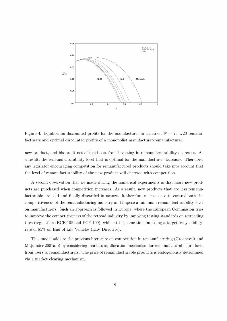
In order to determine the optimal remanufacturability level in presence of competition with
independent remanufacturers, we have to characterize the equilibrium. This task is non-trivial
for a general consumer profile (F, δ), but we are able to analyze the special case of a uniform
distribution of consumer types. In Figure 4, we display the discounted profits for the manufacturer
as a function of the level of remanufacturability, for different levels of competition on the market
for remanufactured products.
Keeping all else equal, a manufacturer is better off without competition on the market for re-
manufactured products. The economic intuition is the following: As the manufacturer does not
make any profit on remanufacturing its products, his incentive to produce a remanufacturable prod-
uct is driven by the residual value of a used remanufacturable product. With increased competition
on the market for remanufactured products, the prices of both remanufactured products and used
remanufacturable products decrease. This limits the price the manufacturer can charge for the
18
MonopolyN=2N=20
0.2
0.21
0.22
0.23
0.24
0.25
0.2 0.4 0.6 0.8 1
q
cn(q)=0.35-0.1ln(1-q)
cr(q)=0
δ=0.25, β=0.55
Vβ
c,M(q)
Figure 4: Equilibrium discounted profits for the manufacturer in a market N = 2, ..., 20 remanu-
facturers and optimal discounted profits of a monopolist manufacturer-remanufacturer.
new product, and his profit net of fixed cost from investing in remanufacturability decreases. As
a result, the remanufacturability level that is optimal for the manufacturer decreases. Therefore,
any legislator encouraging competition for remanufactured products should take into account that
the level of remanufacturability of the new product will decrease with competition.
A second observation that we made during the numerical experiments is that more new prod-
ucts are purchased when competition increases. As a result, new products that are less remanu-
facturable are sold and finally discarded in nature. It therefore makes sense to control both the
competitiveness of the remanufacturing industry and impose a minimum remanufacturability level
on manufacturers. Such an approach is followed in Europe, where the European Commission tries
to improve the competitiveness of the retread industry by imposing testing standards on retreading
tires (regulations ECE 108 and ECE 109), while at the same time imposing a target ‘recyclability’
rate of 85% on End of Life Vehicles (ELV Directive).
This model adds to the previous literature on competition in remanufacturing (Groenevelt and
Majumder 2001a,b) by considering markets as allocation mechanism for remanufacturable products
from users to remanufacturers. The price of remanufacturable products is endogenously determined
via a market clearing mechanism.
19
5 Discussion and Conclusion
In this paper, we develop insights for managers who consider producing a remanufacturable product.
Our model captures some of the key elements driving the decision to introduce a remanufacturable
product, and the subsequent management of the total product line; in particular, we focus on
the market drivers and technology enablers. Motivated by examples from industry, we consider
a market where a remanufactured product is valued less than a new product and is targeted to
the lower end of the market. The proportion of used products that can be remanufactured can be
increased by applying a more expensive production technology.
To our knowledge, this is the first paper to address the integrated market segmentation and
production technology choice problem in a remanufacturing setting. We investigate how these
choices are driven by the characteristics of the market and the cost structure. The existing literature
focuses mainly on operational issues or deals with technology selection (Klausner et al.) and market
segmentation (Ferrer) separately. These two dimensions are strongly coupled via the dependence
of the remanufactured product supply on previous new product sales. Our analysis reveals the
implications of this dependence. Our key results are summarized below.
We study which characteristics of the consumer profile and the production technology make
remanufacturing a profitable strategy. We find that high production costs of the single-use product,
low remanufacturing costs and low incremental costs to make a single-use product remanufacturable
are the key technology drivers. The consumer profile plays a role in the determination of the
profitability of remanufacturing: The more consumers are concentrated on the lower end of the
market, the lower the remanufacturing potential. In addition, the consumer profile and the fixed
cost jointly interact to determine the optimal remanufacturability level: If the fixed cost is higher,
the optimal remanufacturability level is lower, and the market at which this level is attained has
more high-valuation consumers. These results highlight that the consumer profile is a crucial
element in determining the potential for remanufacturing and the optimal remanufacturability
level. Therefore, it would be very useful in practice to invest in understanding the market well
before launching a remanufacturable product.
We identify some important dynamics that can occur during the introduction phase of reman-
ufacturable products. Since a system with remanufactured products is in essence a closed-loop
system, and new and remanufactured products are substitutes, the optimal introduction volumes
show an oscillatory behavior before the stationary regime is reached. The amplitude of the oscilla-
tion of the total demand volume is significantly lower than the amplitude of the oscillation of new
and remanufactured product demand volumes separately. Therefore, common capacity for both
new and remanufactured products is particularly useful in the introduction phase of remanufac-
20
turable products. A model that incorporates capacity considerations can be developed to further
investigate the value of flexible capacity in a remanufacturing environment.
We characterize a specific role of the new product in the portfolio of new and remanufactured
products: New products may be sold in order to generate a supply of remanufactured products,
on which the profit is made. This role is illustrated by the finding that it may be optimal to sell
new products below unit cost. This suggests that manufacturers who also have remanufacturing
operations may benefit from managing both new and remanufactured product lines as part of the
same profit center. Furthermore, a decrease in the unit remanufacturing cost may lead to an
increase in the new product sales volume, in order to supply remanufactured products in response
to increased demand for them. This phenomenon has implications for legislation that provides
subsidies for remanufacturing in order to reduce the total disposal volume.
Finally, we investigate whether the manufacturer would produce a remanufacturable product,
and if so, what remanufacturability level he would choose if used products were remanufactured
and sold by independent competing remanufacturers. We find that the same condition as in the
monopoly case is sufficient for the introduction of a remanufacturable product to be profitable, but
the optimal level of remanufacturability offered by the manufacturer is lower than the monopoly
model and decreases as the number of competing remanufacturers increases.
We conclude with a discussion of the generality and applicability of our results.
We assumed that the ratio of consumer type θ’s willingness-to-pay for remanufactured products
((1 − δ)θ) to his willingness-to-pay for new products (θ) was the same for all consumer types and
equal to 1 − δ, that is, the perceived depreciation δ was homogenous across types. In reality,
it could be that this ratio is different for different consumer types. It is possible to allow for
heterogeneity in perceived depreciation by allowing the willingness-to-pay for a remanufactured
product to be a function v(θ) of the consumer type θ, such that the ratio v(θ)/θ is not constant.
Under some additional assumptions on the shape of v(θ) (concerning the curvature of v (θ) and the
joint interaction between v(θ) and F (θ)), the basic insights remain the same.
We also assumed that there is no cost to dispose of the used products. A unit disposal cost d
can be easily accommodated in our model. If the manufacturer is responsible for disposal, as the
European WEEE directive (2003) on producer responsibility stipulates for example, since all prod-
ucts will eventually be disposed of at the manufacturer’s expense, the problem can be reformulated
with a modified production cost that includes the disposal cost. If the manufacturer disposes only
of returned unusable products, and the consumer disposes of used remanufactured products, a sim-
ilar reformulation is obtained where both the manufacturing cost and the remanufacturing cost are
modified. This is because the maximum price the manufacturer can charge for the remanufactured
product to consumer type θ is then (1 − δ)θ − βd; in other words, the disposal cost is implicitly
21
borne by the manufacturer. The results we obtained are valid if the modified costs satisfy the
cost-related assumptions made in the analysis.
Finally, we assumed that the production costs and underlying market conditions (market size
and perceived depreciation) are constant. The implications of relaxing these assumptions are dis-
cussed below.
We assumed that the costs of manufacturing and remanufacturing are constant over the life
cycle of the product, but in practice, a new technology may become available for either operation.
The sensitivity analysis of §3.4.3 gives us some insight concerning how the optimal product portfolio
would be impacted by a potential decrease in the remanufacturing cost. In particular, our results
indicate that the manufacturer would choose to build a higher remanufacturability level into the
product if he anticipates that the remanufacturing cost will go down in the future. A complete
model that captures beliefs about how costs may evolve over time could potentially be developed
to rigorously model this phenomenon.
In our model, the total market potential is reached from the first period, and is constant over
the time horizon. In practice, it may be that the potential market is progressively penetrated
(Bass 1969), and is controlled via pricing and quality (Kouvelis and Mukhopadhyay 1999), or
constrained by capacity (Ho et al. 2002). In Section 3.3, we showed that interesting but complicated
volume dynamics are created in a remanufacturing context even when the market size for new
products is constant. It is difficult to hypothesize exactly how these dynamics would be affected
by diffusion phenomena without analyzing a specific model of the joint diffusion of both products
in the market over time. Nevertheless, we can hypothesize that if the same market potential is
reached progressively, the investment into the remanufacturability level will not be recouped at the
same rate as in our model and therefore, the remanufacturability level provided will be lower. We
believe that this is a promising avenue for future research.
We further assumed that perceived depreciation is independent of the remanufacturability level
and is constant over time. It may be that the relative willingness-to-pay of a consumer would in-
crease as a function of the remanufacturability level. In addition, as a consumer uses the product,
and learns that remanufactured products provide satisfactory performance, his perceived deprecia-
tion may decrease. Furthermore, the rate of this decrease may depend on the remanufacturability
level of the product, with higher levels resulting in a faster decrease. These phenomena would en-
courage the manufacturer to provide a higher remanufacturability level. Again, a complete model
that captures these phenomena could potentially be developed to investigate their impact in more
detail.
We would like to end with the caveat that although the framework that we developed captures
several important elements that factor into the determination of a remanufacturing strategy, in
22
practice, the market decisions and technology choices are much more complex. Comprehensive
decision support tools to help managers evaluate various options would therefore be very useful.
We hope that our research stimulates such research and development.
6 Acknowledgements
Laurens Debo wishes to thank the Sasakawa Young Leaders Fellowship Fund for financial support
during the last two years of his doctoral studies. The authors gratefully acknowledge the many
insightful comments by three anonymous referees and the Associate Editor.
7 References
Alford, R. 2001. Markets for Retread Used Tires Get Second Life in Budget-conscious Appalachia.
Florida Times Union January 12.
Bass, F.M. 1969. A New Product Growth Model for Consumer Durables. Management Science.
15(5) 215–227.
BIPAVER. 1998. Difficult Tyre Retail Future Ahead. European Rubber Journal May 46–52.
Bozarth, M. 2000a. Radial Truck Tire Retreadability Survey Results. The Tire Retreading/Repair
Journal 44(6) 3–8.
Commission Of The European Communities. 2000. Proposal for a Council Decision on the acces-
sion of the European Community to Regulation 109. Legislation in preparation Commission /*
COM/99/0727 final - AVC 2000/0003 */.
Dhebar, A., S. Oren. 1985. Optimal Dynamic Pricing for Expanding Networks. Marketing Science
4(4) 336–351.
Ferrer, G. 2000. Market Segmentation and Product Line Design in Remanufacturing. Working
paper. The Kenan-Flagler Business School.
Fleischmann, M., J. M. Bloemhof-Ruwaard, R. Dekker, E. van der Laan, J. van Nunen, L. N.
Van Wassenhove. 1997. Quantitative models for reverse logistics: A review. European Journal of
Operational Research 103 (1): 1–17.
23
Fleishmann, M. 2000. Quantitative Models for Reverse Logistics. PhD Thesis, Erasmus University,
Rotterdam.
Fudenberg and Tirole. 1991. Game Theory. MIT Press.
Groenevelt, H., P. Majumder. 2001a. Competition in Remanufacturing. Production and Operations
Management 10(2) 125–141.
Groenevelt, H., P. Majumder. 2001b. Procurement Competition in Remanufacturing. Working
Paper, Simon School of Business, University of Rochester.
Guide, Jr., V. D. R., R. Srivastava, M. Kraus. 1997. Product Structure Complexity and Scheduling
of Operations in Recoverable Manufacturing. International Journal of Production Research 35
3179–3199.
Guide, Jr., V. D. R., S. R. Srivastava. 1998. Inventory Buffers in Recoverable Manufacturing.
Journal of Operations Management 16 551–568.
Ho, T-H., Savin, S., C. Terwiesch. 2002. Managing Demand and Sales Dynamics in New Product
Diffusion Under Supply Constraint. Management Science. 48(2) 187 – 206.
Inderfurth, K. 1998. The Performance of Simple MRP-Driven Policies for Stochastic Manufactur-
ing/Remanufacturing Problems. Working Paper 13/98, University of Magdeburg, Germany.
Inderfurth, K. 2002. Optimal Policies in Hybrid Manufacturing/remanufacturing Systems with
Product Substitution. FEMM working paper 1/2002, University of Magdeburg, Germany.
Kouvelis, P., S. K. Mukhopadhyay. 1999. Modeling the Design Quality Competition for Durable
Products. IIE Transactions. 31(9) 865–880.
Klausner, M., W. M. Grimm, C. Hendrickson. 1998. Reuse of Electric Motors in Consumer
Products. Journal of Industrial Ecology. 2(2) 89–102.
Moorthy, S. 1984. Market Segmentation, Self-Selection, and Product Line Design. Marketing
Science 3(4) 288–308.
Mussa, M., S. Rosen. 1978. Monopoly and Product Quality. Journal of Economic Theory 18
301–317.
Padmanabhan, V., F. M. Bass. 1993. Optimal Pricing of Successive Generations of Product
Advances. International Journal of Research in Marketing 10 185–207.
24
Prejean, M. 1989. Half-soles, Kettles and Cures, Milestones in the Tire Retreading and Repairing
Industry. American Retreaders’ Association.
Savaskan, R. C., S. Bhattacharya, L. N. Van Wassenhove. 1999. Channel Choice and Coordination
in a Remanufacturing Environment. INSEAD Working Paper 99(14/TM).
Smith, J. E., K. F. McCardle. 2002. Structural Properties of Stochastic Dynamic Programs.
Operations Research 50(5) 796–809.
Thierry, M., M. Salomon, J. van Nunen, L. N. Van Wassenhove. 1995. Strategic Issues in Product
Recovery Management. California Management Review 37(2) 114–135.
Toktay, L. B., L. M. Wein, S. A. Zenios. 2000. Inventory Management of Remanufacturable
Products. Management Science 46(11) 1412–1426.
van der Laan E., M. Salomon, R. Dekker, L. N. Van Wassenhove. 1999. Inventory Control in
Hybrid Systems with Remanufacturing. Management Science 45(5) 733 – 747.
Vietor, R. H. K. 1993. Xerox, Design for the Environment. Harvard Business School Case 794–022.
WEEE Directive. 2003. Directive 2002/96/EC of the European Parliament and of the Council of
27 January 2003 on Waste Electrical and Electronic Equipment (WEEE). Official Journal of the
European Union. February 13.
Whang, S. 1995. Market Provision of Custom Software: Learning effects and Low Balling. Man-
agement Science. 41(8) 1343–1352.
8 Appendix
8.1 Some properties of the revenue function
Lemma 4 (i) The Hessian H of the revenue function R(·) is of the form H =
[a + b a
a a
]. (ii)
If F ∈ Fk and n > 0, then a < 0 and b < 0.
Proof. (i) Recall that pN and pR denote the prices of new and remanufactured products, respec-
tively, and that the net utility that a consumer of type θ derives from buying a new product, a re-
manufactured product, and no product, is θ−pN , (1−δ)θ−pR, and 0, respectively. In a given period,
25

consumers choose which product to buy based on the utility that they derive in that period from this
purchase. Let p denote the vector (pN , pR). Then ΩN (p).= θ ∈ [0, 1] : θ − pN ≥ (1 − δ) θ − pR is
the set of consumer types who purchase a new product. ΩR (p) is defined analogously as the set of
consumer types who purchase a remanufactured product. Define the marginal consumers θl(p) and
θh(p) such that θl is indifferent between buying no product and buying a remanufactured product,
and θh is indifferent between buying a remanufactured product and a new product. With the linear
utility structure, if pR were larger than (1 − δ)pN , no remanufactured products would be sold,
and the price pR could be reduced to the level (1 − δ)pN without affecting the demand for either
product. Without loss of generality, we only consider cases where (1− δ)pN ≥ pR in characterizing
the marginal consumers (p ∈ S). In this case, ΩR (p) = [θl(p), θh(p)) and ΩN (p) = [θh(p), 1], where
θl(p) =pR
1 − δand θh(p) =
pN − pR
δ. (A-1)
Let n and r denote the volume of consumers who purchase new and remanufactured products,
respectively, and define ν.= (n, r). Then n =
∫ΩN (p) dF (θ) =
∫ 1θh
f (θ) dθ = 1 − F (θh) = 1 −F (pN−pR
δ ) and r =∫ΩR(p) dF (θ) =
∫ θh
θlf (θ) dθ = F (θh) − F (θl) = F (pN−pR
δ ) − F ( pR
1−δ ).
Taking the derivative of these two equalities with respect to n and r gives
1 = −1δ f(pN−pR
δ
) ∂pN
∂n + 1δ f(pN−pR
δ
) ∂pR
∂n
0 = −1δ f(pN−pR
δ
) ∂pN
∂r + 1δ f(pN−pR
δ
) ∂pR
∂r
0 = 1δ f(pN−pR
δ
) ∂pN
∂n −(
1δ f(pN−pR
δ
)+ 1
1−δf(
pR
1−δ
))∂pR
∂n
1 = 1δ f(pN−pR
δ
) ∂pN
∂r −(
1δ f(pN−pR
δ
)+ 1
1−δf(
pR
1−δ
))∂pR
∂r
The simultaneous solution of these four equations yields ∂pN
∂n = − 1−δf( pR
1−δ )− δ
f(
pN−pRδ
) and ∂pN
∂r =
∂pR
∂r = ∂pR
∂n = − 1−δf( pR
1−δ ).
Since R(ν) = npN (ν) + rpR(ν), we obtain, using the chain rule, that
[∂R∂n , ∂R
∂r
]=
[pN + n∂pN
∂n + r ∂pR
∂n , pR + n∂pN
∂r + r ∂pR
∂r
]=
[pN −
(δ
f(
pN−pRδ
) + 1−δf( pR
1−δ )
)n − 1−δ
f( pR1−δ )
r, pR − 1−δf( pR
1−δ )n − 1−δ
f( pR1−δ )
r
]=
[pN −
(δ
f(θh) + 1−δf(θl)
)(1 − F (θh)) − 1−δ
f(θl)(F (θh) − F (θl)), pR − 1−δ
f(θl)(1 − F (θh)) − 1−δ
f(θl)(F (θh) − F (θl))
].
Define GN (θ).= θ − 1−F (θ)
f(θ) and GR (θ).= (1 − δ)GN (θ). Then some algebraic manipulation
yields [∂R∂n , ∂R
∂r
]=[
δGN (θh) + GR (θl) , GR (θl)]. (A-2)
26
Taking the derivative of ∂R(ν)∂n and ∂R(ν)
∂r with respect to r and n, and following similar steps, we
obtain the elements of the Hessian H:
∂2R
∂n2= δG′
N (θh)∂θh
∂n+ G′
R (θl)∂θl
∂nand
∂2R
∂r2=
∂2R
∂r∂n= G′
R (θl)∂θl
∂r. (A-3)
Since ∂θl
∂n = ∂θl
∂r , we see that H =
[a + b a
a a
]with a = G′
R (θl)∂θl
∂r and b = δG′N (θh) ∂θh
∂n .
(ii) We now specialize this matrix to the case F (θ) = 1 − (1 − θ)κ. For this distribution,
GN (θ) = θ − 1 − θ
κ, (A-4)
so G′N (θ) = 1
κ + 1 and G′R (θ) = (1 − δ)
(1κ + 1
). Since n + r = 1 − F (θl) = (1 − θl)
κ, we have
θl = 1 − (n + r)1κ . Similarly, since n = 1 − F (θh), we have θh = 1 − n
1κ . Therefore,
∂θl
∂r=
∂θl
∂n= −1
κ(n + r)
1κ−1 = −1
κ(1 − θl)
1−κ and∂θh
∂n= −1
κ(1 − θh)1−κ . (A-5)
Substituting, we find
a = −(
1
κ+ 1
)(1 − δ)
1
κ(1 − θl)
1−κ
b = −δ
(1
κ+ 1
)1
κ(1 − θh)1−κ .
n > 0 ⇔ θh < 1 ⇒ b < 0 and a < b since θl ≤ θh.
For future reference, it will be convenient to point out some properties of the Hessian H for the
family of distributions F ∈ Fk when n > 0.
|H| > 0,∂2R
∂n2< 0 (R(·) is strictly concave.) (Property 1)
∂2R
∂n∂r< 0 (New and remanufactured products are imperfect substitutes.) (Property 2)
∂2R
∂r2< 0 (Property 3)
∣∣∣∣∂2R
∂n∂r
∣∣∣∣ <∣∣∣∣∂2R
∂n2
∣∣∣∣ (Property 4)
1
2
∂2R
∂r2>
∂2R
∂n∂r(Property 5)
Remark. These properties hold for any distribution F for which G′N > 0 since this is a sufficient
condition for a and b to be negative. Hence, although our exposition in this paper is for F ∈ Fκ,
our analysis holds for any distribution for which G′N > 0.
27
8.2 Assumptions
A useful condition for characterizing the optimal path is that the solution to (3) is interior to
the feasible region. In addition, to characterize q∗ using first order conditions, we need q∗ < 1.
To this end, we introduce Assumption 1 and Assumption 2, and we provide conditions on model
parameters that assure that Assumption 1 holds if F ∈ Fκ (Lemma 5). We will assume throughout
the derivations that in addition to those assumptions already introduced in the text, the following
assumptions hold:
verify correctness
The maximizer (n∗, r∗) of (3) satisfies n∗ + r∗ < 1. (Assumption 1)
cn (0) < 1, cr (q) < 1 ∀ q and ∃ q < 1 : c (q) < v (q) for q < q. (Assumption 2)
c′′ (q) > 0 and c′n(q) + βqc′r (q) > 0. (Assumption 3)
c′n (q) and c′r (q) are finite for all q ∈ [0, 1]. (Assumption 4)
F ∈ Fκ. (Assumption 5)
Lemma 5 For F ∈ Fκ, there exists κ0 > 0 such that Assumption 1 is satisfied for all κ ∈ (0, κ0).
Proof. The Lagrangian has the form
L = π(n, r) + βv(I + qn − r) + µnn + µrr + λ (1 − n − r) + τ (I − r) .
(r∗, n∗, λ∗, µ∗n, µ∗
r , τ∗) satisfy the K-T conditions:
∂π∂n + qβv′(I + qn − r) + µn − λ = 0
∂π∂r − βv′(I + qn − r) + µr − λ − τ = 0
λ (1 − n − r) = 0, µnn = 0, µrr = 0, τ (I − r) = 0
λ ≥ 0, µn ≥ 0, µr ≥ 0, ν ≥ 0
Assume that r∗ + n∗ = 1 and µ∗n = µ∗
r = 0. Then ∂π∂n(n∗, 1 − n∗) + qβv′(I + qn∗ − r∗) − λ = 0,
or λ = − 1κ(1− δθ∗h) + δθ∗h − cn(q) + qβv′(I + qn∗ − r∗). If κ < 1−δ
[v′(0)+δ−cn(0)]+, then λ < 0, which is
inconsistent with the K-T conditions.
Assume that r∗ + n∗ = 1 and µ∗n = 0, but µ∗
r > 0. Then n∗ = 1, r∗ = 0, and τ∗ = 0. Again,∂π∂n(1, 0) + qβv′(I + q) − λ = 0, or λ = − 1
κ − cn(q) + qβv′(I + q). If κ < 1[v′(0)−cn(0)]+
, then λ < 0,
which is inconsistent with the K-T conditions.
28
Assume that r∗ + n∗ = 1 and µ∗r = 0, but µ∗
n > 0. (i) Assume I ≥ 1. Then n∗ = 0, r∗ = 1, and
τ∗ = 0. In this case, ∂π∂r (0, 1)−βv′(I−1)−λ = 0, or λ = − 1
κ(1−δ)−cr(q)−βv′(I−1) < 0 ∀ κ > 0,
which is inconsistent with the K-T conditions. (ii) Assume I < 1. Then r∗ = 1 contradicts the
K-T condition r∗ ≤ I.
Assume that r∗ + n∗ = 1 and µ∗r > 0, µ∗
n > 0. Then n∗ = r∗ = 0, which contradicts the
assumption r∗ + n∗ = 1.
We conclude that if κ < min( 1−δ[v′(0)+δ−cn(0)]+
, 1[v′(0)−cn(0)]+
), then r∗ + n∗ < 1. It can be shown
that v′(0) < 1− δ − cr(q), so the result is proved with κ0.= min( 1−δ
[1−cr(q)−cn(0)]+, 1
[1−δ−cr(q)−cn(0)]+).
8.3 Proofs
Proof of Lemma 1. Smith and McCardle (2002) consider a Markov decision process of the form
v∗k(xk) = supak∈Akrk(ak, xk) + δkE[v∗k−1(xk−1(ak, xk))] for k > 0, v∗0(x0) = 0. Here, ak and
xk ∈ Θ are the decision variable and the state variable, respectively, in period k. The authors
establish conditions under which the properties of the reward functions rk are inherited by the
value function v∗k. In particular, they prove the following:
Proposition 5 (Smith and McCardle 2002). Let U be the set of functions on X satisfying a C3
(closed convex cone) property P and let P ∗ be a joint extension of P on AxΘ. If, for all k, a) the
reward functions rk(ak, xk) satisfy P ∗ and b) the transitions xk−1(ak, xk) satisfy P ∗(∼U ), then each
v∗k satisfies P and limk→∞ v∗k, if it exists, also satisfies P .
The corresponding variables in our problem are the following: a = ν, A = D ∩ r ≤ I, x = I,
Θ = [0,∞), δ = β, and x = I + qn − r. We would like to show that the value function is concave.
Concavity is a C3 property. The authors show that for convex action and state spaces A and Θ,
joint concavity on AxΘ is a joint extension of concavity on Θ. In our problem, the reward function
rk(νk, Ik) = π(νk) and is independent of Ik. Since π is concave, condition (a) is satisfied. Since
our recursion is deterministic and the transition function is linear, it trivially satisfies condition
(b). In addition, since we have a discounted-cost formulation with a bounded reward function,
Vβ = limk→∞ vk exists. We conclude that Vβ(I; q) is a concave function of I. Note that if the
path (nt, rt), t ≥ 0 is feasible for I0 = I, then it is feasible for any I0 > I. Thus, Vβ (I; q) is
non-decreasing in I. This concludes the proof of part (i). The Hessian H of f(ν, I) with respect
to ν satisfies H11 < 0 and |H| > 0 so f is strictly concave in ν. A unique maximizer of f on A
therefore exists for all t and the optimal path ν∗t = (n∗
t , r∗t ), t ≥ 0 is unique.
Proof of Lemma 2. Part (i): We want to show that if c (q) < v (q), then there exists a feasible
path with a positive discounted profit. We proceed by constructing such a path. Pick ε > 0 and
29
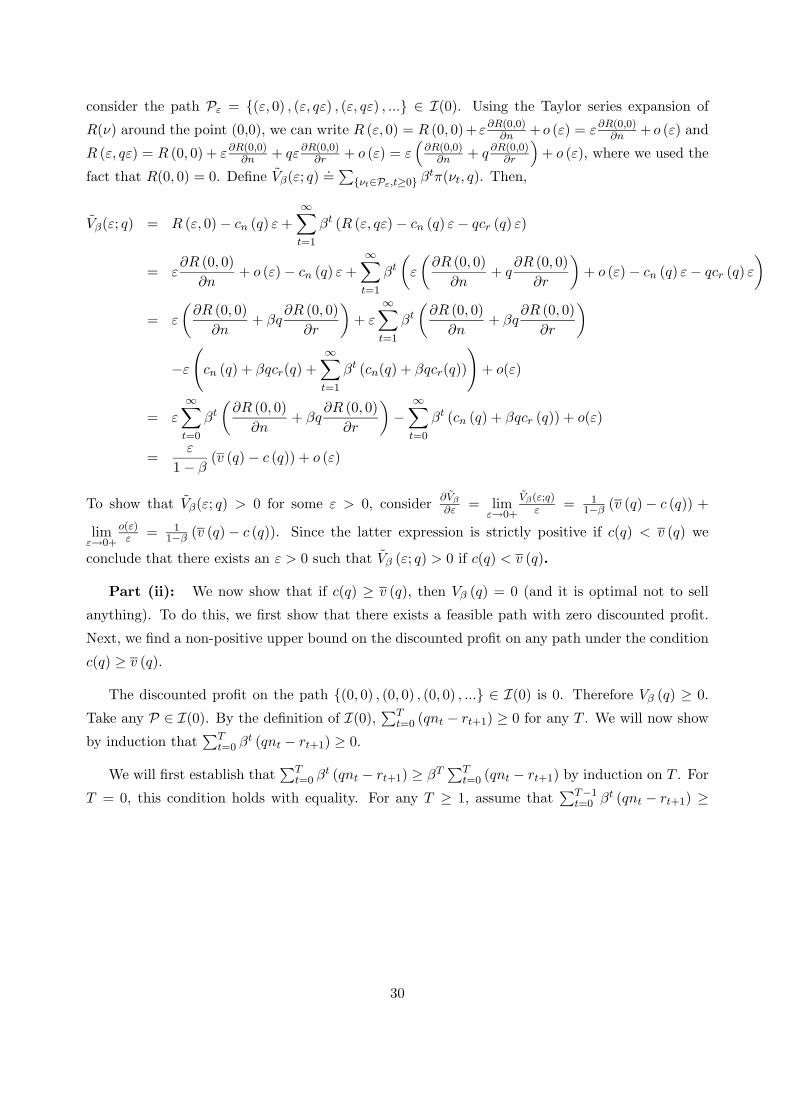
consider the path Pε = (ε, 0) , (ε, qε) , (ε, qε) , ... ∈ I(0). Using the Taylor series expansion of
R(ν) around the point (0,0), we can write R (ε, 0) = R (0, 0)+ ε∂R(0,0)∂n + o (ε) = ε∂R(0,0)
∂n + o (ε) and
R (ε, qε) = R (0, 0) + ε∂R(0,0)∂n + qε∂R(0,0)
∂r + o (ε) = ε(
∂R(0,0)∂n + q ∂R(0,0)
∂r
)+ o (ε), where we used the
fact that R(0, 0) = 0. Define Vβ(ε; q).=∑
νt∈Pε,t≥0 βtπ(νt, q). Then,
Vβ(ε; q) = R (ε, 0) − cn (q) ε +
∞∑
t=1
βt (R (ε, qε) − cn (q) ε − qcr (q) ε)
= ε∂R (0, 0)
∂n+ o (ε) − cn (q) ε +
∞∑
t=1
βt
(ε
(∂R (0, 0)
∂n+ q
∂R (0, 0)
∂r
)+ o (ε) − cn (q) ε − qcr (q) ε
)
= ε
(∂R (0, 0)
∂n+ βq
∂R (0, 0)
∂r
)+ ε
∞∑
t=1
βt
(∂R (0, 0)
∂n+ βq
∂R (0, 0)
∂r
)
−ε
(cn (q) + βqcr(q) +
∞∑
t=1
βt (cn(q) + βqcr(q))
)+ o(ε)
= ε∞∑
t=0
βt
(∂R (0, 0)
∂n+ βq
∂R (0, 0)
∂r
)−
∞∑
t=0
βt (cn (q) + βqcr (q)) + o(ε)
=ε
1 − β(v (q) − c (q)) + o (ε)
To show that Vβ(ε; q) > 0 for some ε > 0, consider∂Vβ
∂ε = limε→0+
Vβ(ε;q)ε = 1
1−β (v (q) − c (q)) +
limε→0+
o(ε)ε = 1
1−β (v (q) − c (q)). Since the latter expression is strictly positive if c(q) < v (q) we
conclude that there exists an ε > 0 such that Vβ (ε; q) > 0 if c(q) < v (q).
Part (ii): We now show that if c(q) ≥ v (q), then Vβ (q) = 0 (and it is optimal not to sell
anything). To do this, we first show that there exists a feasible path with zero discounted profit.
Next, we find a non-positive upper bound on the discounted profit on any path under the condition
c(q) ≥ v (q).
The discounted profit on the path (0, 0) , (0, 0) , (0, 0) , ... ∈ I(0) is 0. Therefore Vβ (q) ≥ 0.
Take any P ∈ I(0). By the definition of I(0),∑T
t=0 (qnt − rt+1) ≥ 0 for any T . We will now show
by induction that∑T
t=0 βt (qnt − rt+1) ≥ 0.
We will first establish that∑T
t=0 βt (qnt − rt+1) ≥ βT∑T
t=0 (qnt − rt+1) by induction on T . For
T = 0, this condition holds with equality. For any T ≥ 1, assume that∑T−1
t=0 βt (qnt − rt+1) ≥
30
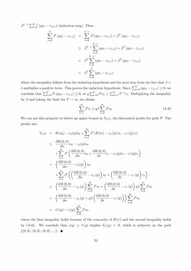
βT−1∑T−1
t=0 (qnt − rt+1) (induction step). Then
T∑
t=0
βt (qnt − rt+1) =T−1∑
t=0
βt (qnt − rt+1) + βT (qnt − rt+1)
≥ βT−1T−1∑
t=0
(qnt − rt+1) + βT (qnt − rt+1)
= βTT−1∑
t=0
(qnt − rt+1) + βT (qnt − rt+1)
= βTT∑
t=0
(qnt − rt+1) ,
where the inequality follows from the induction hypothesis and the next step from the fact that β <
1 multiplies a positive term. This proves the induction hypothesis. Since∑T
t=0 (qnt − rt+1) ≥ 0, we
conclude that∑T
t=0 βt (qnt − rt+1) ≥ 0, or q∑T
t=0 βtnt ≥∑T
t=1 βt−1rt. Multiplying the inequality
by β and taking the limit for T → ∞, we obtain
∞∑
t=1
βtrt ≤ qβ∞∑
t=0
βtnt. (A-6)
We can use this property to derive an upper bound on Vβ,P , the discounted profits for path P. The
profits are:
Vβ,P = R (ν0) − cn(q)n0 +∞∑
t=1
βt (R (νt) − cn (q) nt − cr (q) rt)
≤ ∂R (0, 0)
∂nn0 − cn(q)n0
+∞∑
t=1
βt
(∂R (0, 0)
∂nnt +
∂R (0, 0)
∂rrt − cn(q)nt − cr(q)rt
)
=
(∂R (0, 0)
∂n− cn(q)
)n0
+∞∑
t=1
βt
((∂R (0, 0)
∂n− cn (q)
)nt +
(∂R (0, 0)
∂r− cr (q)
)rt
)
≤(
∂R (0, 0)
∂n− cn (q)
) ∞∑
t=0
βtnt +
(∂R (0, 0)
∂r− cr (q)
)qβ
∞∑
t=0
βtnt
=
(∂R (0, 0)
∂n− cn (q) + qβ
(∂R (0, 0)
∂r− cr (q)
)) ∞∑
t=0
βtnt
= (v (q) − c (q))∞∑
t=0
βtnt.
where the first inequality holds because of the concavity of R (ν) and the second inequality holds
by (A-6). We conclude that c(q) ≥ v (q) implies Vβ (q) = 0, which is achieved on the path
(0, 0) , (0, 0) , (0, 0) , ....
31
Proof of Lemma 3. Consider the path Pq = (ns, 0) , (n, r) , (n, r) , (n, r) ... ∈ I(0) and let
Vβ,P (q) denote corresponding discounted profit on this path. We have that ∂R(n,r)∂n = cn (q) and
∂R(ns,0)∂n = cn (q). Hence, ∂R(ns,0)
∂n = ∂R(n,r)∂n . By Property 1 and Property 2, ∂R(n,r)
∂n is a strictly
decreasing function of r and n. Therefore, either n = ns and r = 0 or n < ns and r > 0. Then,
I1 = qns ≥ qn ≥ r. As qn ≥ r, we have that It+1 = It + qn − r ≥ It ∀t. Since I1 ≥ r, it follows
that It ≥ r ∀t and P ∈ I(0). By the definition of ns and (n, r), the elements of policy P achieve
the optimal profit over the feasible region in each period starting with the initial condition I0 = 0.
Therefore, P achieves the optimal profit: Vβ,P (q) = Vβ(q).
We will show that the derivative of Vβ,P (q) with respect to q is negative. V ′β,P (q) =
∑∞t=0 βt ∂π(νt,q)
∂q .∂π(ns,0,q)
∂q = ∂π∂n
∂ns
∂q + ∂π∂q = ∂π
∂q = −c′n(q)ns, where we used ∂π(ns,0)n = 0. ∂π(νt,q)
∂q = ∂π∂n
∂n∂q + ∂π
∂r∂r∂q + ∂π
∂q =∂π∂q = −c′n(q)n−c′r(q)r ∀t ≥ 1 where we used
(∂π∂n , ∂π
∂r
)= (0, 0) by the definition of (n, r). Summing,
we find that V ′β,P (q) = −c′n (q)
(ns + n β
1−β
)− c′r (q) r β
1−β ; Assumption 4 assures that the sum
converges. Since ns ≥ n, V ′P,β (q) ≤ −c′n (q) n 1
1−β − c′r (q) r β1−β . By assumption, c′n (q) > 0. If, in
addition, c′r (q) = 0, then V ′P,β (q) < 0. If c′r (q) < 0, then V ′
P,β (q) ≤ (−c′n (q) − βqc′r (q)) n 11−β since
r ≤ qn. Invoking Assumption 3, we again obtain V ′P,β (q) < 0.
Lemma 6 Assume c (q) < v (q). Recall that the policy function g (I) = I + qn∗ (I) − r∗ (I) and
consider the interval X = [0, g (0)]. Then, g(I) > 0 for I ∈ X and either
(i) g′ (I) < 0, |g′ (I)| < 1 and r∗ (I) = I for I ∈ X, or
(ii) there exists I ∈ X such that g′ (I) < 0, |g′ (I)| < 1 and r∗ (I) = I for I ∈ [0, I], and g′ (I) ≥ 0,
r∗ (I) < I for I ∈ (I, g (0)]. In addition, if qn < r, g(I) < I on (I, g(0)].
Proof In this lemma, we prove that the policy function g has one of the two forms shown in Figure
6 (decreasing or U-shaped on [0, g(0)], which is the relevant interval, as we shall show.
For notational simplicity, we suppress the dependence of π(ν, q) and Vβ(I, q) on q in this proof.
We make the following conjecture concerning (n∗ (I) , r∗ (I)): There exists an interval [0, I] on
which n∗ (I) > 0 and r∗ (I) = I, i.e. there exists an interval over which the constraint r ≤ I in
(3) is binding. Assuming that the conjecture is correct, we characterize n∗ (I) and g (I) in Step
1a. We validate the conjecture in Step 1b, and determine whether it holds for the entire interval
[0, g (0)]. If so, then part (i) is proven with I = g(0); otherwise, we determine the exact interval
[0, I] for which the conjecture holds. We make a second conjecture concerning (n∗ (I) , r∗ (I)): On
(I, g (0)], n∗ (I) > 0 and 0 < r∗ (I) < I . Steps 2a and 2b characterize g′ under these assumptions
and validate this conjecture, respectively, proving part (ii).
Step 1a: Characterization of n∗ (I) and g (I) under the conjecture r∗ (I) = I and n∗ (I) > 0
on [0, I].
32
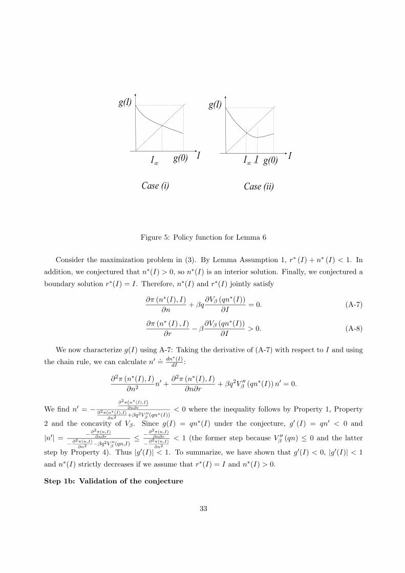
I
g(I)
g(0) I
g(I)
g(0)I I I
Case (i) Case (ii)
Figure 5: Policy function for Lemma 6
Consider the maximization problem in (3). By Lemma Assumption 1, r∗ (I) + n∗ (I) < 1. In
addition, we conjectured that n∗(I) > 0, so n∗(I) is an interior solution. Finally, we conjectured a
boundary solution r∗(I) = I. Therefore, n∗(I) and r∗(I) jointly satisfy
∂π (n∗(I), I)
∂n+ βq
∂Vβ (qn∗(I))
∂I= 0. (A-7)
∂π (n∗ (I) , I)
∂r− β
∂Vβ (qn∗(I))
∂I> 0. (A-8)
We now characterize g(I) using A-7: Taking the derivative of (A-7) with respect to I and using
the chain rule, we can calculate n′ .= dn∗(I)
dI :
∂2π (n∗(I), I)
∂n2n′ +
∂2π (n∗(I), I)
∂n∂r+ βq2V ′′
β (qn∗(I)) n′ = 0.
We find n′ = −∂2π(n∗(I),I)
∂n∂r
∂2π(n∗(I),I)
∂n2 +βq2V ′′β
(qn∗(I))< 0 where the inequality follows by Property 1, Property
2 and the concavity of Vβ . Since g(I) = qn∗(I) under the conjecture, g′ (I) = qn′ < 0 and
|n′| =− ∂2π(n,I)
∂n∂r
− ∂2π(n,I)
∂n2 −βq2V ′′β
(qn,I)≤ − ∂2π(n,I)
∂n∂r
− ∂2π(n,I)
∂n2
< 1 (the former step because V ′′β (qn) ≤ 0 and the latter
step by Property 4). Thus |g′(I)| < 1. To summarize, we have shown that g′(I) < 0, |g′(I)| < 1
and n∗(I) strictly decreases if we assume that r∗(I) = I and n∗(I) > 0.
Step 1b: Validation of the conjecture
33
We now need to show that there exists a range [0, I] on which n∗(I) > 0 and A-8 is satisfied.
Let us take the derivative of the two terms in A-8 with respect to I. We find ∂∂I
(∂π(n∗(I),I)
∂r
)=
∂2π∂n∂rn′ + ∂2π
∂2r=
|H|+βq ∂2π
∂2rV ′′
β(qn∗)
∂2π
∂n2 +βqV ′′β
(qn∗)< 0 and ∂
∂I
(βV ′
β (qn∗ (I)))
= βqV ′′β (qn∗ (I)) n′ > 0. A-8 holds at
I = 0. As the first term in (A-8) strictly decreases in I and the second term strictly increases in
I, one of the following two cases is true on [0, g(0)]: either (i) A-8 holds ∀I ∈ [0, g(0)] or (ii) there
exists I ∈ (0, g(0)] for which A-8 is satisfied at equality. Expressing this more precisely, we have
one of the following two cases:
(i) ∂π(n∗(g(0)),g(0))∂r − βV ′
β (qn∗ (g(0))) > 0. Then g′(I) < 0, |g′(I)| < 1 and n∗(I) strictly decreases
on X = [0, g(0)]. Since |g′(I)| < 1, we have g (g(0)) > 0, that is, n∗(g(0)) > 0 (since g = qn∗ on
this range) which, together with the fact that n∗(I) strictly decreases on this range, validates the
conjecture that n∗ (I) > 0 over [0, g (0)].
(ii) There exists I.= sup
(I : ∂π(n∗(I),I)
∂r − βV ′β (qn∗ (I)) > 0
)< g(0). The conjecture that r∗ (I) = I
on [0, I] is validated with I = I since A-8 holds on [0, I), with equality holding only at I = I. Then
g′(I) < 0, |g′(I)| < 1 and n∗(I) strictly decreases on [0, I].
Step 2a: Characterization of g′(I) under the conjecture 0 < r∗ (I) < I and n∗ (I) > 0 on
(I, g (0)]
We now complete case (ii) by characterizing (n∗ (I) , r∗ (I)) over (I, g(0)]. We conjecture that
0 < r∗ (I) < I and n∗ (I) > 0 for I ∈ (I, g(0)]. In this case, n∗(I) and r∗(I) satisfy the first order
conditions of the right hand side of (3):
∂π (n∗(I), r∗(I))
∂n+ βq
∂Vβ (g(I))
∂I= 0. (A-9)
∂π (n∗ (I) , r∗(I))
∂r− β
∂Vβ (g(I))
∂I= 0. (A-10)
We also know that Vβ, n∗, r∗ jointly satisfy Vβ (I) = π (n∗ (I) , r∗ (I)) + βVβ (g (I)) with g(I) =
I + qn∗(I) − r∗(I). Taking the derivative of this expression with respect to I gives V ′β(I) =
∂π∂nn′ + ∂π
∂r r′ + βV ′β(g(I))g′(I) (with r′
.= dr∗(I)
dI ). Taking the derivative of g(I) and evaluating it at
(n∗(I), r∗(I)) gives g′(I) = 1 + qn′ − r′. Substituting g′(I) in the previous expression, collecting
terms, and simplifying using A-9 and A-10, we find
V ′β (I) = βV ′
β (g (I)) . (A-11)
V ′′β (I) = βV ′′
β (g (I)) g′ (I) . (A-12)
By Lemma 1, V ′β (I) ≥ 0. First consider the case V ′
β (I) = 0. By (A-11), if V ′β (I) = 0, we have
V ′β (g (I)) = 0. Then, by A-9 and A-10 and the definition of ν, (n∗ (I) , r∗(I)) = (n, r). Thus,
g (I) = I + qn − r, and g′ (I) = 1 > 0. Note that if qn < r, then g(I) < I.
34
Next consider the case V ′β (I) > 0. By (A-11), if V ′
β (I) > 0, then, as β < 1, we must have
that V ′β (g (I)) > V ′
β (I), and by the concavity of Vβ , g (I) < I. We conclude that if qn < r, then
g(I) < I on (I, g(0)].
To characterize g′(I) when V ′β (I) > 0, consider the following three subcases:
(a) V ′′β (g (I)) < 0 and V ′′
β (I) < 0. Since 0 < β < 1, and A-12 must hold, g′(I) > 0.
(b) V ′′β (g (I)) < 0 and V ′′
β (I) = 0. Since β > 0 and A-12 must hold, g′(I) = 0.
(c) V ′′β (g (I)) = 0. Taking the derivative of A-9 and A-10 with respect to I and using
V ′′β (g (I)) = 0 gives a system of two equations in the two unknowns n′(I) and r′(I) whose only
solution is n′(I) = 0 and r′(I) = 0. In this case, g′(I) = 1 > 0.
Thus, we conclude that g′(I) ≥ 0 on (I, g(0)].
Step 2b: Validation of the conjecture
We will first determine the sign of n′ and r′. Taking the derivative of (A-9) and (A-10) with
respect to I, we obtain
(∂2π∂n2 + βq2 ∂2Vβ
∂I2
)n′ +
(∂2π∂n∂r − βq
∂2Vβ
∂I2
)r′ = −qβ
∂2Vβ
∂I2(∂2π∂r∂n − βq
∂2Vβ
∂I2
)n′ +
(∂2π∂r2 + β
∂2Vβ
∂I2
)r′ = β
∂2Vβ
∂I2
(A-13)
from which we solve for (n′, r′):
[n′
r′
]=
β∂2Vβ
∂I2
|H| + β(
∂2π∂n2 + q2 ∂2π
∂r2 + 2q ∂2π∂n∂r
)∂2Vβ
∂I2
[−q ∂2π
∂r2 − ∂2π∂n∂r
q ∂2π∂n∂r + ∂2π
∂n2
].
The signs of each term can easily be determined:∂2Vβ
∂I2 ≤ 0, |H|+β(
∂2π∂n2 + q2 ∂2π
∂r2 + 2 ∂2π∂n∂rq
)∂2Vβ
∂I2 ≥0, −q ∂2π
∂r2 − ∂2π∂n∂r > 0 and q ∂2π
∂n∂r + ∂2π∂n2 < 0 by Lemma 1, Property 2, Property 3 and Property 4.
Therefore, n′ ≤ 0, r′ ≥ 0 and |n′| = −n′. Showing that |n′| < 1 is equivalent to showing that
β
(q (1 − q)
∂2π
∂r2+ (1 − 2q)
∂2π
∂n∂r− ∂2π
∂n2
)∂2Vβ
∂I2< |H| . (A-14)
With Property 5 we obtain
q (1 − q)∂2π
∂r2+ (1 − 2q)
∂2π
∂n∂r>
∂2π
∂n∂r,
and with Property 4, we obtain further that
q (1 − q)∂2π
∂r2+ (1 − 2q)
∂2π
∂n∂r>
∂2π
∂n2.
Together with∂2Vβ
∂I2 < 0 and |H| > 0, we have that (A-14) is satisfied. We conclude that |n′| < 1.
35
Since r∗ (I) = I > 0 and we have proven that r′ ≥ 0 on (I, g(0)], we conclude that r∗ (I) > 0 on
(I, g(0)]. However, since we have proven that n′ < 0, it is not as immediate that n∗ (I) > 0 ∀I ∈(I, g(0)]. On the other hand, as |n′| < 1 both on (I, g(0)] and on [0, I] (by part i), we have that
n∗ (g(0)) > 0. Because n′ < 0 on [0,g(0)], we conclude that n∗(I) > 0 on (I, g(0)] is also verified.
Lemma 7 Define ν∞.= (n∞, r∞) ∈ D simultaneously satisfying ∂R(ν∞)
∂n + qβ ∂R(ν∞)∂r = c (q) and
qn∞ = r∞. If c (q) < v (q) and qn < r, then,
(i) There exists a unique I∞ ∈ [0, g(0)] such that I∞ solves g (I) = I. In addition, g′(I∞) < 0 and
|g′(I∞)| < 1. Moreover, r∞ = I∞.
(ii) The region [g(I), I] is a capture region, that is, It ∈ [g(I), I] implies that It+1 = g(It) ∈ [g(I), I].
(iii) Starting with I0 = 0, there exists a Tq ≥ 0 such that r∗t = It ∀t ≥ Tq. Moreover, limt→∞It =
I∞.
Proof Part (i): We start by conjecturing that there exists I∞ such that g (I∞) = I∞, g′(I∞) < 0
and |g′(I∞)| < 1. Then, I∞ = g(I∞) = I∞ + qn∗(I∞) − r∗(I∞), implying that
qn∗(I∞) = r∗(I∞). (A-15)
By Lemma 6, we know that g′(I∞) ≤ 0 and |g′(I∞)| < 1 if and only if r∗(I∞) = I∞, so under the
above conjecture, I∞ satisfies A-7:
∂π (n∗(I∞), I∞)
∂n+ βq
∂Vβ (qn∗(I∞))
∂I= 0. (A-16)
Also recall from Lemma 6 that Vβ(I) = π (n∗(I), I) + βVβ (qn∗(I))) for any I such that r∗(I) = I.
Using the chain rule, V ′β(I) = ∂π
∂n∂n∗
∂I + ∂π∂r + βqV ′
β(qn∗(I))∂n∗
∂I = ∂n∗
∂I (∂π∂n + βqV ′
β(qn∗(I))) + ∂π∂r = ∂π
∂r
where the last equality follows by substituting A-7. In particular, under the above conjecture, this
equality holds for I = I∞, yielding
V ′β(I∞) =
∂π(n∗(I∞), I∞)
∂r(A-17)
In addition, since I∞ = r∗(I∞) = qn∗(I∞),
V ′β(qn∗(I∞)) =
∂π(n∗(I∞), qn∗(I∞))
∂r. (A-18)
Substituting this equation in A-16, we find:
∂π (n∗(I∞), qn∗(I∞))
∂n+ qβ
∂π (n∗(I∞), qn∗(I∞))
∂r= 0. (A-19)
Consider N (n).= ∂π(n,qn)
∂n +qβ ∂π(n,qn)∂r . As N ′ (n) = ∂2π(n,qn)
∂n2 +q ∂2π(n,qn)∂n∂r +qβ
(∂2π(n,qn)
∂n∂r + q ∂2π(n,qn)∂r2
)<
0 since all terms are negative, the solution to (A-19), if it exists, is unique. Now, we show that such
36

a solution exists. N (0) = v (q) − c(q) by definition. Since v (q) > c(q) we have N(0) > 0. Note
that n ∈ [0, 11+q ], as n + qn ≤ 1. Thus, if we show that N( 1
1+q ) < 0, then, we will have proven that
N (n) = 0 has a unique solution n such that n > 0 and n+qn < 1. It can be shown that if κ < 1−δδ ,
then ∂π(n,1−n)∂n + qβ ∂π(n,1−n)
∂r < 0. The proof of Lemma 5 develops conditions on κ that satisfy this
inequality. Noting that at n = 11+q , r = 1−n, we conclude that
∂π( 11+q
, q
1+q)
∂n + qβ∂π(∂π( 1
1+q, q
1+q)
∂r < 0,
which can be rewritten as N( 11+q ) < 0. We further conclude that n∗(I∞) solving A-19 is unique
and that (n∗(I∞), qn∗(I∞)) ∈ int(D). In addition, since dn∗(I)dI < 0 in this range (as shown in the
proof of part (i) in Lemma 6), I∞ is unique.
Recall that ν∞.= (n∞, r∞) satisfying ∂π(ν∞)
∂n + qβ ∂π(ν∞)∂r = 0, qn∞ = r∞ and ν∞ ∈ D simulta-
neously. Comparing A-15 and A-19 with the definition of ν∞, and noting that (n∗(I∞), qn∗(I∞)) ∈int(D), we conclude that n∞ = n∗(I∞) and r∞ = r∗(I∞) under the conjecture. In addition, since
I∞ = r∗(I∞) under the conjecture, we have that r∞ = I∞.
We now need to show that the conjecture is true. By Lemma 6, I∞ satisfies the conjecture if∂π(n∗(I∞),I∞)
∂r −βV ′β (qn∗ (I∞)) > 0, or, using A-15 and substituting A-18, if (1 − β) ∂π(n∗(I∞),qn∗(I∞))
∂r >
0, or, since β > 0,∂π (n∗ (I∞) , qn∗ (I∞))
∂r> 0. (A-20)
Let the functions r (n) and r (n) be defined by ∂π(n,r(n))∂n = 0 and ∂π(n,r(n))
∂r = 0. Consider Figure 6.
We will show that if qn < r, then the solution to (A-19) lies on the segment determined by r = qn,
r < r (n), and r > r(n) (marked in bold in Figure 6), and that on this segment, ∂π(n,qn)∂r > 0. In
this case, I∞ satisfies the conjecture.
Since R (ν) is concave, (n, r) is the unique intersection point of r (n) and r (n). Note that by
differentiating ∂π(n,r(n))∂n = 0 and ∂π(n,r(n))
∂r = 0, we obtain ∂2π(n,r(n))∂n2 + ∂2π(n,r(n))
∂n∂r∂r(n)
∂n = 0 and∂2π(n,r(n))
∂n∂r + ∂2π(n,r(n))∂r2
∂r(n)∂n = 0. Evaluating these expressions at n = n and using the fact that
r(n) = r(n) = r, we find ∂r(n)∂n = −
∂2π(n,r)∂n∂r
∂2π(n,r)
∂r2
and ∂r(n)∂n = −
∂2π(n,r)
∂n2
∂2π(n,r)∂n∂r
. It follows that
∣∣r′ (n)∣∣ <
∣∣r′ (n)∣∣⇔
∂2π(n,r)∂n∂r
∂2π(n,r)∂r2
<
∂2π(n,r)∂n2
∂2π(n,r)∂n∂r
⇔ 0 <∂2π∗
∂n2
∂2π∗
∂r2− ∂2π∗
∂n∂r
∂2π∗
∂n∂r= |H|
which is true by Property 1. Therefore, r (n) crosses r (n) from above, validating Figure 6. Thus,
for n > n, we have r (n) < r (n). As r > qn, it follows that the line r = qn lies below the point
(n, r), further validating Figure 6. Furthermore, as ∂2π∂n∂r < 0 we have that ∂π(n,r)
∂n < 0 for r > r (n)
and ∂π(n,r)∂r > 0 for r < r (n). Therefore, on the segment determined by r = qn, r < r (n), and
r > r(n), marked in bold in Figure 6, we have that ∂π(n,r)∂n < 0 and ∂π(n,r)
∂r > 0. A-19 and A-20
being simultaneously satisfied means that the first term of (A-19) must be negative and the second
term must be positive. Therefore, the solution (n∞, qn∞) to (A-19) lies on the segment determined
by r = qn, r < r (n), and r > r(n). Thus, from (A-20), it follows that I∞ satisfies the conjecture.
37
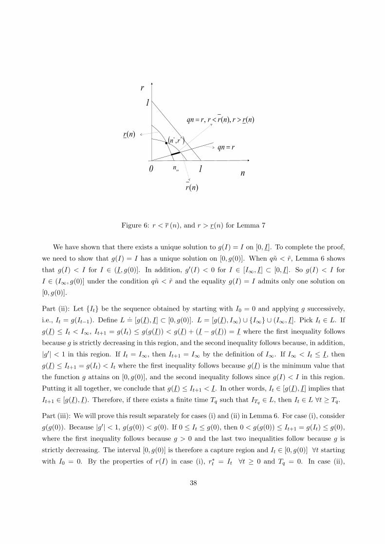
n
r
10
1
** ,rn
sun
)(nr
)(nr
rqn
)(),(, nrrnrrrqn
Figure 6: r < r (n), and r > r(n) for Lemma 7
We have shown that there exists a unique solution to g(I) = I on [0, I]. To complete the proof,
we need to show that g(I) = I has a unique solution on [0, g(0)]. When qn < r, Lemma 6 shows
that g(I) < I for I ∈ (I, g(0)]. In addition, g′(I) < 0 for I ∈ [I∞, I] ⊂ [0, I]. So g(I) < I for
I ∈ (I∞, g(0)] under the condition qn < r and the equality g(I) = I admits only one solution on
[0, g(0)].
Part (ii): Let It be the sequence obtained by starting with I0 = 0 and applying g successively,
i.e., It = g(It−1). Define L.= [g(I), I] ⊂ [0, g(0)]. L = [g(I), I∞) ∪ I∞ ∪ (I∞, I]. Pick It ∈ L. If
g(I) ≤ It < I∞, It+1 = g(It) ≤ g(g(I)) < g(I) + (I − g(I)) = I where the first inequality follows
because g is strictly decreasing in this region, and the second inequality follows because, in addition,
|g′| < 1 in this region. If It = I∞, then It+1 = I∞ by the definition of I∞. If I∞ < It ≤ I, then
g(I) ≤ It+1 = g(It) < It where the first inequality follows because g(I) is the minimum value that
the function g attains on [0, g(0)], and the second inequality follows since g(I) < I in this region.
Putting it all together, we conclude that g(I) ≤ It+1 < I. In other words, It ∈ [g(I), I] implies that
It+1 ∈ [g(I), I). Therefore, if there exists a finite time Tq such that ITq ∈ L, then It ∈ L ∀t ≥ Tq.
Part (iii): We will prove this result separately for cases (i) and (ii) in Lemma 6. For case (i), consider
g(g(0)). Because |g′| < 1, g(g(0)) < g(0). If 0 ≤ It ≤ g(0), then 0 < g(g(0)) ≤ It+1 = g(It) ≤ g(0),
where the first inequality follows because g > 0 and the last two inequalities follow because g is
strictly decreasing. The interval [0, g(0)] is therefore a capture region and It ∈ [0, g(0)] ∀t starting
with I0 = 0. By the properties of r(I) in case (i), r∗t = It ∀t ≥ 0 and Tq = 0. In case (ii),
38
g(I0) = g(0) > I. We need to prove that there exists a Tq such that It > I if 1 ≤ t ≤ Tq − 1,
and ITq ∈ [g(I), I]. To prove this, let us start by supposing that no such Tq exists. Then I < It ≤g(0) ∀t ≥ 1. In this region, It+1 = g(It) < It, so It is a strictly decreasing sequence. Because
this sequence is in the bounded interval I < It ≤ g(0), it must converge to I, that is, limt→∞It = I.
However, I cannot be a limit point of this sequence since g(I) < I. By contradiction, it cannot
be true that I < It ≤ g(0) ∀t ≥ 1, and there exists a finite Tq such that ITq ≤ I. In addition,
since g increasing on (I, g(0)], g(I) ≥ g(I) ∀I ∈ (I, g(0)], so ITq = g(ITq−1) ≥ g(I). We therefore
conclude that there exists a finite Tq such that ITq ∈ [g(I), I]. By (ii), It ∈ [g(I), I] ∀t ≥ Tq and
r∗t = It by the properties of r∗(I) on [0, I] in case (ii) of Lemma 6. Finally, since I∞ ≤ min(g(0), I)
is the unique point such that g(I) = I, limt→∞It = I∞.
Proof of Proposition 1: The proof of this proposition draws on Lemma 6 which characterizes
the policy function g when c(q) < v(q) and on Lemma 7 that characterizes the optimal path when
c(q) < v(q) and qn < r.
Derivation of (4). From Lemmas 2 and 3, it follows that we can restrict our attention to cases
where q ∈ Q and from Lemma 7, it follows that we can split problem (1) in two parts when
qn < r. In particular, for t ≥ Tq, we can focus on solutions of the form rt = It and It+1 = g(It) =
It + qnt − rt = qnt. For simplicity, the feasible region is suppressed in the maximization problems
below.
Vβ (q).= max
Tq−1∑
t=0
βtπ (nt, rt, q) + βTqVβ
(ITq , q
), (A-21)
where
Vβ
(ITq , q
) .= max
∞∑
τ=0
βτπ(nTq+τ , ITq+τ , q
)
= max
(π(nTq , ITq , q
)+
∞∑
τ=0
βτ+1π(nTq+τ+1, qnTq+τ , q
))
(A-22)
and
ITq = qn0 +
Tq−1∑
t=1
(qnt − rt) (A-23)
We now establish (4) in two steps, first for the case where t ≥ Tq and then for the case 0 ≤ t < Tq.
In the case that Tq = 0, the part 0 ≤ t < Tq can be omitted.
Taking the derivative of Vβ (I, q) with respect to I and evaluating it at I = ITq , we obtain:
∂
∂IVβ
(ITq , q
)=
∂π(n∗
Tq, ITq , q
)
∂r(A-24)
Taking the derivative of the sum in the right-hand side of (A-22) with respect to nTq+τ and
using the chain rule for τ ≥ 0, we obtain first order conditions that are satisfied by the optimal
39
sequence ν∗t , t ≥ Tq:
βτ∂π(n∗
Tq+τ , r∗Tq+τ
)
∂n+ βτ+1q
∂π(n∗
Tq+τ+1, r∗Tq+τ+1
)
∂r= 0, for τ = 0, 1, ... (A-25)
or, equivalently,
∂R(n∗
T+τ , r∗T+τ
)
∂n+ βq
∂R(n∗
T+τ+1, r∗T+τ+1
)
∂r= c (q) , for τ = 0, 1, ... (A-26)
We have thus established (4) for t ≥ Tq. Let us now turn to t < Tq. Taking the derivative of
the sum in A-21 with respect to nt, t = 0, 1, ..Tq − 1, we obtain βt ∂π(nt,rt)∂n + βTq
∂Vβ(ITq ,q)∂I
∂ITq
∂nt=
βt ∂π(nt,rt)∂n + qβTq
∂Vβ(ITq ,q)∂I , t = 0, 1, ..Tq−1, where the equality follows because
∂ITq
∂nt= q by the
definition of ITq in A-23.
Similarly, taking the derivative of the sum in A-21 with respect to rt, t = 1, 2, ..Tq−1, we obtain
βt ∂π(nt,rt)∂r + βTq
∂Vβ(ITq ,q)∂I
∂ITq
∂rt= βt ∂π(nt,rt)
∂r − βTq∂Vβ(ITq ,q)
∂I , t = 1, 2, ..Tq−1.
The optimal sequence ν∗t , t = 0, 1, . . . , Tq − 1 satisfies the first order conditions obtained by
equating these expressions to 0. Using r∗0 = 0, A-24 and dividing through by βt, we can write:
∂π(n∗t ,r∗t ,q)∂n + qβTq−t
∂π(n∗
Tq,r∗Tq
,q)
∂r = 0, t = 0, 1, ..., Tq − 1
∂π(n∗t ,r∗t ,q)∂r − βTq−t
∂π(n∗
Tq,r∗Tq
,q)
∂r = 0, t = 1, 2, ..., Tq − 1
Substituting the second set of equalities into the first set, we find
∂π (n∗t , r
∗t , q)
∂n+ q
∂π (n∗t , r
∗t , q)
∂r, t = 0, 1, 2, . . . , Tq − 1. (A-27)
From the second set of equalities, we find that
βTq−t∂π(n∗
Tq, ITq , q
)
∂r=
∂π (n∗t , r
∗t , q)
∂r= β
∂π(n∗
t+1, r∗t+1, q
)
∂r, t = 1, ..., Tq − 1 (A-28)
Substituting in (A-27), we obtain
∂π (n∗t , r
∗t , q)
∂n+ qβ
∂π(n∗
t+1, r∗t+1, q
)
∂r, t = 0, 1, 2, . . . , Tq − 1
Thus, we have
∂R (n∗t , r
∗t )
∂n+ βq
∂R(n∗
t+1, r∗t+1
)
∂r= c (q) for t = 0, 1, ..., Tq − 1, (A-29)
Together with (A-26), we obtain (4).
Derivation of (5). We again proceed in two parts. For t ≥ Tq, we focus on solutions of the
form rt = It and It+1 = g(It) = It + qnt − rt = qnt. It is convenient to define the following
40

recursive relationship for t ≥ Tq: Vβ (It, q) = max0≤nt+It≤1
[π (nt, It, q) + βVβ (qnt, q)]. Let n∗(It) =
argmax0≤nt+It≤1
[π (nt, It, q) + βVβ (qnt, q)]. By Assumption 1, we are assured that n∗ is an interior solution
and satisfies the first-order condition∂[π(nt,It,q)+βVβ(qnt,q)]
∂n = 0. We can further write Vβ (It, q) =
π (n∗t , It, q) + βVβ (qn∗
t , q) ∀t ≥ Tq.
Taking the derivative of this expression with respect to q for each t ≥ Tq, and simplifying using
the first order conditions satisfied by n∗t , we obtain
βτ ∂Vβ
(ITq+τ , q
)
∂q− βτ+1 ∂Vβ
(ITq+τ+1, q
)
∂q= βτ
∂π(n∗
Tq+τ , ITq+τ , q)
∂q+ βτ+1 ∂Vβ
(ITq+τ+1, q
)
∂In∗
Tq+τ
for τ ≥ 0. Adding these equalities over τ ≥ 0 and taking the limit as τ → ∞, we obtain
∂Vβ
(ITq , q
)
∂q=
∞∑
τ=0
βτ
∂π(n∗
Tq+τ , ITq+τ , q)
∂q+ β
∂Vβ
(ITq+τ+1, q
)
∂In∗
Tq+τ
.
By definition, π(n∗Tq+τ , ITq+τ , q) = R(n∗
Tq+τ , ITq+τ ) − cn(q)n∗t+τ − cr(q)r
∗t+τ , so
∂π(n∗T+τ ,IT+τ ,q)
∂q =
−c′n(q)n∗t+τ − c′r(q)r
∗t+τ . In addition,
∂π(n∗T+τ ,IT+τ ,q)
∂r =∂R(n∗
T+τ ,IT+τ )
∂r − cr(q). Using (A-24),
∂
∂IVβ
(ITq+τ+1, q
)=
∂π(n∗
Tq+τ+1, ITq+τ+1, q)
∂r. (A-30)
Putting these two together, we find
∂Vβ
(ITq , q
)
∂q=
∞∑
τ=0
βτ
β
∂R(n∗
Tq+τ+1, r∗Tq+τ+1, q
)
∂r− βcr (q) − c′n (q)
n∗
Tq+τ − c′r (q) r∗Tq+τ
(A-31)
We now turn to t < Tq. Let us first rewrite A-21: Vβ (q) =∑Tq−1
t=0 βtπ (n∗t , r
∗t , q)+βTqVβ
(ITq , q
)=
∑Tq−1t=0 βtπ (n∗
t , r∗t , q) + βTqVβ
(qn∗
0 +∑Tq−1
t=1 (qn∗t − r∗t ) , q
). We find
∂Vβ (q)
∂q=
Tq−1∑
t=0
βt ∂π (n∗t , r
∗t , q)
∂q+ βTq
∂Vβ(ITq , q)
∂I
Tq−1∑
t=0
n∗t + βTq
∂Vβ(ITq , q)
∂q
where we usedd(I0+
∑Tq−1t=0 (qn∗
t−r∗t ),q)
dq =∑Tq−1
t=0 n∗t . Collecting terms, and using A-24 and A-31, we
obtain
∂Vβ (q)
∂q=
Tq−1∑
t=0
βt
βTq−t
∂π(n∗
Tq, ITq , q
)
∂r− c′n (q)
n∗
t − c′r (q) r∗t
+βTq
∞∑
τ=0
βτ
β
∂π(n∗
Tq+τ+1, ITq+τ+1, q)
∂r− c′n (q)
n∗
Tq+τ − c′r (q) r∗Tq+τ
41
or with (A-28) we obtain:
∂Vβ (q)
∂q=
Tq−1∑
t=0
βt
((β
∂π(n∗
t+1, r∗t+1, q
)
∂r− c′n (q)
)n∗
t − c′r (q) r∗t
)
+βTq
∞∑
τ=0
βτ
β
∂π(n∗
Tq+τ+1, ITq+τ+1, q)
∂r− c′n (q)
n∗
Tq+τ − c′r (q) r∗Tq+τ
Finally, we can rewrite the previous expression using the definition π (n, r, q) = R (n, r)− cn (q) n−cr (q) r:
∂Vβ (q)
∂q=
Tq−1∑
t=0
βt
((β
∂R(n∗
t+1, r∗t+1
)
∂r− βcr (q) − c′n (q)
)n∗
t − c′r (q) r∗t
)
+βTq
∞∑
τ=0
βτ
β
∂R(n∗
Tq+τ+1, ITq+τ+1
)
∂r− βcr (q) − c′n (q)
n∗
Tq+τ − c′r (q) r∗Tq+τ
.
Note that the terms in the latter expression have the same structure for 0 ≤ t < Tq as well as for
Tq ≤ t. Thus, we have obtained (5):
∂Vβ (q)
∂q=
∞∑
t=0
βt
((β
∂R(n∗
t+1, r∗t+1
)
∂r− βcr (q) − c′n (q)
)n∗
t − c′r (q) r∗t
).
Proof of Proposition 2:
The function Vβ(q) was defined exclusive of the initial fixed investment cost k(q); the discounted
profit at time 0 equals Vβ(q)− k(q). A sufficient condition for the existence of a q∗ > 0 is therefore
V ′β(0) − k′(0) > 0.
Let us evaluate V ′β(0). As q = 0, and I0 = 0, we have that r∗t = 0 ∀t ≥ 0. Evaluating (4) at
q = 0 gives∂R(ν∗
t )∂n = c (0) ∀t ≥ 0. By the definition of nsu, ν∗
t = (nsu, 0) ∀t ≥ 0. Evaluating (5) at
q = 0 and ν∗t = (nsu, 0) ∀t ≥ 0, we find
V ′β (0) =
1
1 − β
(β
(∂R (nsu, 0)
∂r− cr (0)
)− c′n (0)
)nsu.
We will use Lemma 4 to evaluate ∂R(nsu,0)∂r . Since the case r = 0 corresponds to having θh = θl,
using A-2, we have [∂R(nsu,0)∂n , ∂R(nsu,0)
∂r ] = [GN (θh) , GR (θh)], or, ∂R(nsu,0)∂r = (1 − δ) ∂R(nsu,0)
∂n by
the definition of GR. Therefore,
V ′β (0) =
1
1 − β
(β
((1 − δ)
∂R (nsu, 0)
∂n− cr (0)
)− c′n (0)
)nsu.
Since by definition, ∂R(nsu,0)∂n = cn (0), we obtain V ′
β (0) = 11−β (β(1 − δ) cn(0) − cr (0) − c′n (0))nsu.
It follows that ∆.= V ′
β(0)− k′(0) = 11−β (β(1 − δ) cn(0) − cr (0) − c′n (0))nsu − k′(0) > 0 is a suf-
ficient condition for q∗ > 0.
42
Proof of Proposition 3. We first derive dnsu
dκ . If β (1 − δ) cn (0) − cr (0) > c′n (0), the sign
of d∆dκ is identical to the sign of dnsu
dκ . By definition, nsu is determined by ∂R(nsu,0)∂n = cn (0).
For F (θ) = 1 − (1 − θ)κ ∈ Fκ, the marginal consumer, θsu, is defined by nsu = (1 − θsu)κ.
From A-2, we know that ∂R(nsu,0)∂n = GN (θsu). Using A-4, we obtain θsu − 1−θsu
κ = cn (0)
or θsu = 1+cn(0)κ1+κ . Plugging θsu into nsu = (1 − θsu)κ, we obtain nsu =
((1−cn(0))κ
1+κ
)κ. Fi-
nally, dnsu
dκ =(
(1−cn(0))κ1+κ
)κ (ln(
(1−cn(0))κ1+κ
)+ 1
1+κ
). Since the first term is non-negative, we ob-
tain that dnsu
dκ < 0 if and only if cn (0) > 1 − 1+κκ e−1/(1+κ). As 0 > 1 − 1+κ
κ e−1/(1+κ) and
cn (0) ≥ 0, the latter condition is always satisfied. This completes our proof that dnsu
dκ < 0,
or, that d∆dκ < 0 if β (1 − δ) cn (0) − cr (0) > c′n (0). We now consider d∆
dcn(0) .d∆
dcn(0) = β(1 −δ)nsu(cn(0)) + (β (1 − δ) cn (0) − cr (0) − c′n (0)) dnsu
dcn(0) . The first term is positive. dnsu
dcn(0) =
−κ( (1−cn(0))κ1+κ )κ−1 κ
1+κ < 0. We conclude that depending on the magnitude of dnsu
dcn(0) ,d∆
dcn(0) could
be either positive or negative.
Proof of Proposition 4. Recall that∂π(n∗
t ,r∗t )∂n + βq
∂π(n∗t+1,r∗t+1)∂r = 0 ∀t (4). With Lemma 7, we
know that ν∞ = (n∞, qn∞) = ν∗(I∞) exists and is unique. Following Stokey and Lucas (1989,
section 6.4), we approximate the previous expression using Taylor series expansion around ν∞ for
t ≥ Tq. We obtain the following second order linear difference equation:
0 =∂2π (n∞, qn∞)
∂n2(n∗
t − n∞) +∂2π (n∞, qn∞)
∂n∂r(r∗t − qn∞)
+βq∂2π (n∞, qn∞)
∂r∂n
(n∗
t+1 − n∞
)+ βq
∂2π (n∞, qn∞)
∂r2
(r∗t+1 − qn∞
).
Recall that r∗t = It and qn∗t = r∗t+1 for t ≥ Tq (Lemma 7). Let us define zt
.= n∗
t − n∞. Then, the
previous equation can be written as:(
∂2π (n∞, qn∞)
∂n2+ βq2 ∂2π (n∞, qn∞)
∂r2
)zt+q
∂2π (n∞, qn∞)
∂n∂rzt−1+βq
∂2π (n∞, qn∞)
∂r∂nzt+1 = 0,∀t ≥ Tq
(A-32)
with zTq−1 =ITq
q − n∞. The solution of A-32 is of the form zt = azt−Tqa + bz
t−Tq
b where za and zb
are the roots of the characteristic equation(
∂2π (n∞, qn∞)
∂n2+ βq2 ∂2π (n∞, qn∞)
∂r2
)z + q
∂2π (n∞, qn∞)
∂n∂r+ βq
∂2π (n∞, qn∞)
∂r∂nz2 = 0. (A-33)
Note that, by definition of π(ν) the Hessian of π(ν) is equal to the Hessian of R(ν). Let us define
R∞.= R (n∞, qn∞). Then
za,b =−(∂2R∞
∂n2 + βq2 ∂2R∞
∂r2 ) ±√(
∂2R∞
∂n2 + βq2 ∂2R∞
∂r2
)2− 4βq2
(∂2R∞
∂n∂r
)2
2βq ∂2R∞
∂n∂r
= −γ ±√
γ2 − 1β
with γ.= 1
2βq
∂2R∞
∂n2 +βq2 ∂2R∞
∂r2
∂2R∞∂n∂r
. The roots za and zb are real if√
β > 1γ , or
√β(
∂2R∞
∂n2 + βq2 ∂2R∞
∂r2
)<
2βq ∂2R∞
∂n∂r , or ∂2R∞
∂n2 + βq2 ∂2R∞
∂r2 − 2√
βq ∂2R∞
∂n∂r < 0. The latter inequality can be rewritten as
43
[1,−√
βq]H
[1
−√βq
]< 0 with H =
[∂2R∞
∂n2∂2R∞
∂n∂r∂2R∞
∂n∂r∂2R∞
∂r2
]. Remember that H is negative definite.
Therefore we conclude that the inequality is satisfied and the roots of (A-33) are real. In addition,
both roots are negative with zb < za. Note that zazb =(−γ +
√γ2 − 1
β
)(−γ −
√γ2 − 1
β
)= 1
β ,
from which it follows that |zb| = 1β|za|
. Hence, if |za| < 1, then |zb| > 1. Let us now show that
|za| < 1. Since za < 0, |za| = γ −√
γ2 − 1β . |za| − 1 < 0 ⇔ γ − 1 <
√γ2 − 1
β ⇔ q (β + 1) ∂2R∞
∂n∂r >
∂2R∞
∂n2 + βq2 ∂2R∞
∂r2 . The left-hand side of the last inequality is linear in β. It is satisfied for β = 0,
as q ∂2R∞
∂n∂r > ∂2R∞
∂n2 by Property 4. It is also satisfied for β = 1, as 0 > ∂2R∞
∂n2 + q2 ∂2R∞
∂r2 − 2q ∂2R∞
∂n∂r =[
1 −q]H
[1
−q
], which is negative since H is negative definite. We conclude that |za| < 1,
|zb| > 1 and that limt→∞
∣∣ztb
∣∣ = +∞. Since zt = azt−Tqa + bz
t−Tq
b and n∗t and n∞ are finite, we
must have that b = 0. Consequently, n∗t = n∞ + azt−Tq . The constant a is determined using
the boundary condition zTq−1 =ITq
q − n∞: a = za(ITq
q − n∞). If Tq = 0, the linearization A-32
holds for all t ≥ 0 with initial condition I0 = 0, which yields a = −zan∞. Therefore, we obtain
n∗t = n∞
(1 − zt+1
a
)t ≥ 0.
We will now evaluate γ for F ∈ Fκ. Since the marginal consumers (θl,∞, θh,∞) corresponding
to ν∞ satisfy n∞ = 1 − F (θh,∞) and r∞ = F (θh,∞) − F (θl,∞), we obtain
γ =1
2βq
((G′
N (θh,∞) − G′R (θh,∞))
∂θh,∞
∂n + G′R (θl,∞)
∂θl,∞
∂n
G′R (θl,∞)
∂θl,∞
∂r
+ βq2
)
from (A-3). As F ∈ Fκ we can use (A-4) and (A-5) to obtain
γ =1
2βq
(−δ 1
κ (1 − θh,∞)1−κ − (1 − δ) 1κ (1 − θl,∞)1−κ
− (1 − δ) 1κ (1 − θl,∞)1−κ + βq2
).
With (A-15), which, written as a function of (θl,∞, θh,∞) is equivalent to1−θh,∞
1−θl,∞= (1 + q)−
1κ , we
obtain
γ =1
2βq
(δ
1 − δ(1 + q)−
1κ(1−κ) + 1 + βq2
).
Finally, note that when κ = 1, R (ν) is a quadratic function and the linearization is thus exact.
Proof of Proposition 5. This proof is done in two steps. First, we characterize an approximation
of q∗ for β ≈ 1. Second, we show how this approximation depends on κ. In previous results
developed for a given remanufacturability level q, ν∗t was determined for q, but this dependence
was suppressed in the notation. From now on, we work with q∗, so ν∗t is determined for q∗. We
again suppress this dependence in the notation.
Step 1a. Approximate characterization of q∗:
44
Since r∗0 = 0, we can rewrite (5), evaluated at q∗, as
∂Vβ (q∗)
∂q= (1 − β)
∞∑
t=0
βt
((β
∂R(n∗
t+1, r∗t+1
)
∂r− βcr (q∗) − c′n (q∗)
)n∗
t − βc′r (q∗) r∗t+1
).
Multiplying this equation by 1 − β, and separating it into two parts, we obtain
(1 − β)∂Vβ (q∗)
∂q= (1 − β)
Tq−1∑
t=0
βt
((β
∂R(n∗
t+1, r∗t+1
)
∂r− βcr (q∗) − c′n (q∗)
)n∗
t − βc′r (q∗) r∗t+1
)
+ (1 − β)∞∑
t=Tq
βt
((β
∂R(n∗
t+1, q∗n∗
t
)
∂r− βcr (q∗) − c′n (q∗)
)n∗
t − βq∗c′r (q∗)n∗t
).
We find that limβ→1− (1 − β)∂Vβ(q∗)
∂q
= limβ→1− (1 − β)∞∑
t=Tq
βt
((β
∂R(n∗
t+1, q∗n∗
t
)
∂r− βcr (q∗) − c′n (q∗)
)n∗
t − βq∗c′r (q∗) n∗t
)
since the first term above is finite. q∗ satisfies the first-order condition∂Vβ(q)
∂q = k′ (q), or,
(1 − β)∂Vβ(q∗)
∂q = (1 − β) k′ (q∗). Then limβ→1− (1 − β)∂Vβ(q∗)
∂q = 0. From the previous expres-
sion, we have
limβ→1− (1 − β)∞∑
t=Tq
βt
((β
∂R(n∗
t+1, q∗n∗
t
)
∂r− βcr (q∗) − c′n (q∗)
)n∗
t − βq∗c′r (q∗) n∗t
)= 0, or,
limβ→1− (1 − β)∞∑
t=Tq
βt
(β
∂R(n∗
t+1, q∗n∗
t
)
∂r− c′ (q∗)
)n∗
t = 0. (A-34)
We approximate∂R(n∗
t+1,q∗n∗t )
∂r around ν∗∞ = (n∗
∞, q∗n∗∞)
.= ν∗(I∞(q∗)) using Taylor series expan-
sion:
∂R(n∗
t+1, q∗n∗
t
)
∂r=
∂R∞
∂r+
∂2R∞
∂r∂n
(n∗
t+1 − n∞
)+ q∗
∂2R∞
∂r2(n∗
t − n∗∞) + o(||ν∗
t+1 − ν∗∞||), (A-35)
where R∞.= R(ν∗
∞). Substituting into A-34 and collecting terms, we find
0 = limβ→1−(1 − β)
(β
∂R∞
∂r− c′ (q∗)
) ∞∑
t=Tq
βtn∗t
+limβ→1− (1 − β)∞∑
t=Tq
βt+1
(∂2R∞
∂r∂n
(n∗
t+1 − n∗∞
)+ q∗
∂2R∞
∂r2(n∗
t − n∗∞) + o(||ν∗
t+1 − ν∗∞||)
)n∗
t .
From Lemma 6, we have that at I, (A-7) is satisfied and (A-8) is satisfied with equality, therefore∂π(n∗(I),I)
∂n +q ∂π(n∗(I),I)∂r = 0. Remember from Lemma 7 that ∂π(n∗(I∞),I∞)
∂n +qβ ∂π(n∗(I∞),I∞)∂r = 0 with
I∞ = qn∗(I∞) (A-19). Therefore, as β → 1−, I → I∞. Thus for t ≥ Tq,(n∗
t+1, q∗n∗
t
)→ (n∗
∞, q∗n∗∞)
45
as β → 1− and the second term in parentheses converges to 0 in the last equality. Since n∗t > 0 ∀t,
expressing the dependence of q∗ on the parameter β with the expression q∗β, we conclude that the
following must hold for the first term to also be equal to 0:
limβ→1−
β∂R∞
(n∗∞, q∗βn∗
∞
)
∂r− c′
(q∗β)
= 0.
Therefore, for β ≈ 1, β∂R∞(n∗
∞,q∗βn∗∞)
∂r ≈ c′(q∗β). Let q∗ be such that
β∂R∞ (n∗
∞, q∗n∗∞)
∂r= c′(q∗). (A-36)
q∗ approximates the optimal remanufacturability level q∗. With (A-19) evaluated at q∗, we obtain
∂R∞ (n∗∞, q∗n∗
∞)
∂n+ q∗β
∂R∞ (n∗∞, q∗n∗
∞)
∂r= c (q∗) ,
which, with (A-36) gives∂R∞ (n∗
∞, q∗n∗∞)
∂n= c (q∗) − q∗c′ (q∗) . (A-37)
In conclusion, (A-36) and (A-37) approximately determine (q∗, n∗∞). This completes our approxi-
mate characterization of q∗.
We will now specialize this characterization to F ∈ F κ. The marginal consumers(θ∞,∗l , θ∞,∗
h
)
are defined by n∗∞ =
(1 − θ∞,∗
h
)κand r∗∞ =
(1 − θ∞,∗
l
)κ −(1 − θ∞,∗
h
)κfor F ∈ Fκ. We can rewrite
(A-36) and (A-37) as a function of(θ∞,∗l , θ∞,∗
h , q∗):
βGR
(θ∞,∗l
)= c′ (q∗) and δGN
(θ∞,∗h
)+ GR
(θ∞,∗l
)= c (q∗) − q∗c′ (q∗) .
Furthermore, we can write A-15 as a function of(θ∞,∗l , θ∞,∗
h , q∗):
(1−θ∞,∗l
)κ
(1−θ∞,∗h
)κ = 1 + q∗. Defining
cl (q).= c′(q)
β and ch (q).= c (q) − (1 + βq) c′(q)
β , we obtain that the triple(θ∞,∗l , θ∞,∗
h , q∗)
satisfies
the following conditions:
(1 − δ)GN (θl) = cl (q) and δGN (θh) = ch (q) (A-38)
1 − θl
1 − θh= (1 + q)
1κ . (A-39)
With Lemma 4, we have that GN (θ) = θ − 1−θκ . Substituting in (A-38), solving for (θl, θh) and
substituting these expressions into A-39, we find that the following condition that must be satisfied
by q∗:
1 − cl(q)1−δ
1 − ch(q)δ
= (1 + q)1κ . (A-40)
This completes our approximate characterization of q∗ for F ∈ Fκ and β ≈ 1.
Step 2. Characterizing q∗ as a function of κ.
46
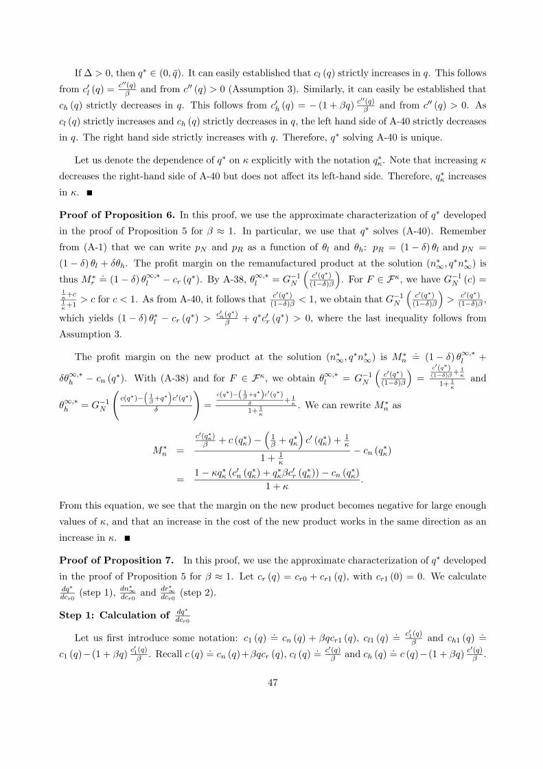
If ∆ > 0, then q∗ ∈ (0, q). It can easily established that cl (q) strictly increases in q. This follows
from c′l (q) = c′′(q)β and from c′′ (q) > 0 (Assumption 3). Similarly, it can easily be established that
ch (q) strictly decreases in q. This follows from c′h (q) = − (1 + βq) c′′(q)β and from c′′ (q) > 0. As
cl (q) strictly increases and ch (q) strictly decreases in q, the left hand side of A-40 strictly decreases
in q. The right hand side strictly increases with q. Therefore, q∗ solving A-40 is unique.
Let us denote the dependence of q∗ on κ explicitly with the notation q∗κ. Note that increasing κ
decreases the right-hand side of A-40 but does not affect its left-hand side. Therefore, q∗κ increases
in κ.
Proof of Proposition 6. In this proof, we use the approximate characterization of q∗ developed
in the proof of Proposition 5 for β ≈ 1. In particular, we use that q∗ solves (A-40). Remember
from (A-1) that we can write pN and pR as a function of θl and θh: pR = (1 − δ) θl and pN =
(1 − δ) θl + δθh. The profit margin on the remanufactured product at the solution (n∗∞, q∗n∗
∞) is
thus M∗r
.= (1 − δ) θ∞,∗
l − cr (q∗). By A-38, θ∞,∗l = G−1
N
(c′(q∗)(1−δ)β
). For F ∈ Fκ, we have G−1
N (c) =1κ+c
1κ+1
> c for c < 1. As from A-40, it follows that c′(q∗)(1−δ)β < 1, we obtain that G−1
N
(c′(q∗)(1−δ)β
)> c′(q∗)
(1−δ)β ,
which yields (1 − δ) θ∗l − cr (q∗) > c′n(q∗)β + q∗c′r (q∗) > 0, where the last inequality follows from
Assumption 3.
The profit margin on the new product at the solution (n∗∞, q∗n∗
∞) is M∗n
.= (1 − δ) θ∞,∗
l +
δθ∞,∗h − cn (q∗). With (A-38) and for F ∈ Fκ, we obtain θ∞,∗
l = G−1N
(c′(q∗)(1−δ)β
)=
c′(q∗)(1−δ)β
+ 1κ
1+ 1κ
and
θ∞,∗h = G−1
N
(c(q∗)−
(1β
+q∗)c′(q∗)
δ
)=
c(q∗)−( 1β
+q∗)c′(q∗)δ
+ 1κ
1+ 1κ
. We can rewrite M∗n as
M∗n =
c′(q∗κ)β + c (q∗κ) −
(1β + q∗κ
)c′ (q∗κ) + 1
κ
1 + 1κ
− cn (q∗κ)
=1 − κq∗κ (c′n (q∗κ) + q∗κβc′r (q∗κ)) − cn (q∗κ)
1 + κ.
From this equation, we see that the margin on the new product becomes negative for large enough
values of κ, and that an increase in the cost of the new product works in the same direction as an
increase in κ.
Proof of Proposition 7. In this proof, we use the approximate characterization of q∗ developed
in the proof of Proposition 5 for β ≈ 1. Let cr (q) = cr0 + cr1 (q), with cr1 (0) = 0. We calculatedq∗
dcr0(step 1), dn∗
∞
dcr0and dr∗∞
dcr0(step 2).
Step 1: Calculation of dq∗
dcr0
Let us first introduce some notation: c1 (q).= cn (q) + βqcr1 (q), cl1 (q)
.=
c′1(q)β and ch1 (q)
.=
c1 (q)−(1 + βq)c′1(q)
β . Recall c (q).= cn (q)+βqcr (q), cl (q)
.= c′(q)
β and ch (q).= c (q)−(1 + βq) c′(q)
β .
47
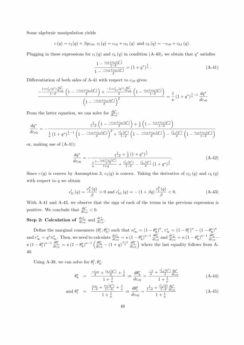
Some algebraic manipulation yields
c (q) = c1(q) + βqcr0, cl (q) = cr0 + cl1 (q) and ch (q) = −cr0 + ch1 (q) .
Plugging in these expressions for cl (q) and ch (q) in condition (A-40), we obtain that q∗ satisfies
1 − cr0+cl1(q∗)
1−δ
1 − −cr0+ch1(q∗)δ
= (1 + q∗)1κ . (A-41)
Differentiation of both sides of A-41 with respect to cr0 gives:
−1+c′l1(q∗) dq∗
dcr01−δ
(1 − −cr0+ch1(q∗)
δ
)+
−1+c′h1(q∗) dq∗
dcr0δ
(1 − cr0+cl1(q∗)
1−δ
)
(1 − −cr0+ch1(q∗)
δ
)2 =1
κ(1 + q∗)
1κ−1 dq∗
dcr0
From the latter equation, we can solve for dq∗
dcr0:
dq∗
dcr0= −
11−δ
(1 − −cr0+ch1(q∗)
δ
)+ 1
δ
(1 − cr0+cl1(q
∗)1−δ
)
1κ (1 + q∗)
1κ−1(1 − −cr0+ch1(q∗)
δ
)2+
c′l1(q∗)
1−δ
(1 − −cr0+ch1(q∗)
δ
)− c′
h1(q∗)
δ
(1 − cr0+cl1(q∗)
1−δ
)
or, making use of (A-41):
dq∗
dcr0= −
11−δ + 1
δ (1 + q∗)1κ
1κ
1−cr0+cl1(q∗)
1−δ
1+q +c′l1(q∗)
1−δ − c′h1(q∗)
δ (1 + q∗)1κ
. (A-42)
Since c (q) is convex by Assumption 3, c1(q) is convex. Taking the derivative of cl1 (q) and ch (q)
with respect to q we obtain
c′l1 (q) =c′′1 (q)
β> 0 and c′h1 (q) = − (1 + βq)
c′′1 (q)
β< 0. (A-43)
With A-41 and A-43, we observe that the sign of each of the terms in the previous expression is
positive. We conclude that dq∗
dcr0< 0.
Step 2: Calculation of dn∗∞
dcr0and dr∗∞
dcr0.
Define the marginal consumers (θ∗l , θ∗h) such that n∗
∞ = (1 − θ∗h)κ, r∗∞ = (1 − θ∗l )κ − (1 − θ∗h)κ
and r∗∞ = q∗n∗∞. Then, we need to calculate dn∗
∞
dcr0= κ (1 − θ∗h)κ−1 dθ∗
h
dcr0and dr∗∞
dcr0= κ (1 − θ∗h)κ−1 dθ∗
h
dcr0−
κ (1 − θ∗l )κ−1 dθ∗
l
dcr0= κ (1 − θ∗h)κ−1
(dθ∗
h
dcr0− (1 + q)
κ−1κ
dθ∗l
dcr0
)where the last equality follows from A-
40.
Using A-38, we can solve for θ∗l , θ∗h:
θ∗h =−cr0
δ + ch1(q∗)
δ + 1κ
1 + 1κ
⇒ dθ∗hdcr0
=−1δ +
c′h1(q∗)
δdq∗
dcr0
1 + 1κ
(A-44)
and θ∗l =
cr01−δ + cl1(q∗)
(1−δ) + 1κ
1 + 1κ
⇒ dθ∗ldcr0
=1
1−δ +c′l1(q)1−δ
dq∗
dcr0
1 + 1κ
(A-45)
48
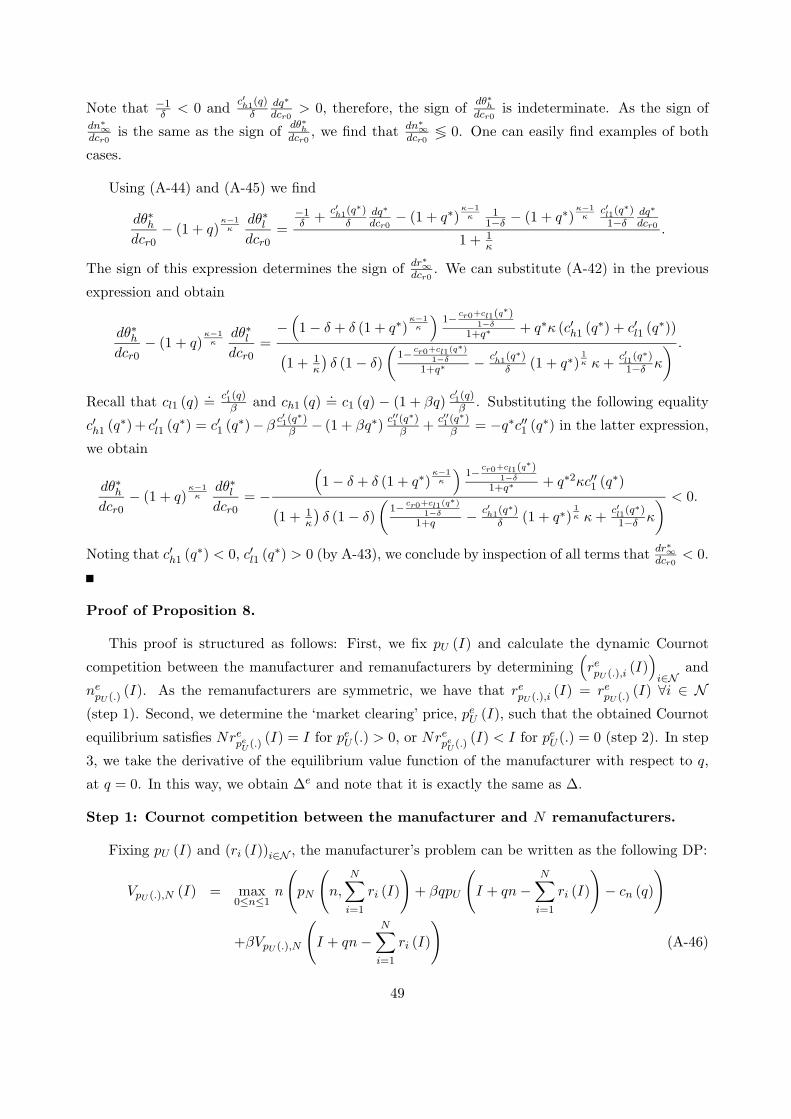
Note that −1δ < 0 and
c′h1(q)
δdq∗
dcr0> 0, therefore, the sign of
dθ∗h
dcr0is indeterminate. As the sign of
dn∗∞
dcr0is the same as the sign of
dθ∗h
dcr0, we find that dn∗
∞
dcr0≶ 0. One can easily find examples of both
cases.
Using (A-44) and (A-45) we find
dθ∗hdcr0
− (1 + q)κ−1
κdθ∗ldcr0
=−1δ +
c′h1(q
∗)δ
dq∗
dcr0− (1 + q∗)
κ−1κ 1
1−δ − (1 + q∗)κ−1
κc′l1(q∗)1−δ
dq∗
dcr0
1 + 1κ
.
The sign of this expression determines the sign of dr∗∞dcr0
. We can substitute (A-42) in the previous
expression and obtain
dθ∗hdcr0
− (1 + q)κ−1
κdθ∗ldcr0
=−(1 − δ + δ (1 + q∗)
κ−1κ
)1−
cr0+cl1(q∗)1−δ
1+q∗ + q∗κ (c′h1 (q∗) + c′l1 (q∗))
(1 + 1
κ
)δ (1 − δ)
(1−
cr0+cl1(q∗)
1−δ
1+q∗ − c′h1(q∗)
δ (1 + q∗)1κ κ +
c′l1(q∗)
1−δ κ
) .
Recall that cl1 (q).=
c′1(q)β and ch1 (q)
.= c1 (q) − (1 + βq)
c′1(q)β . Substituting the following equality
c′h1 (q∗)+ c′l1 (q∗) = c′1 (q∗)−βc′1(q
∗)β − (1 + βq∗)
c′′1 (q∗)β +
c′′1 (q∗)β = −q∗c′′1 (q∗) in the latter expression,
we obtain
dθ∗hdcr0
− (1 + q)κ−1
κdθ∗ldcr0
= −
(1 − δ + δ (1 + q∗)
κ−1κ
)1−
cr0+cl1(q∗)1−δ
1+q∗ + q∗2κc′′1 (q∗)
(1 + 1
κ
)δ (1 − δ)
(1−
cr0+cl1(q∗)
1−δ
1+q − c′h1(q∗)
δ (1 + q∗)1κ κ +
c′l1(q
∗)
1−δ κ
) < 0.
Noting that c′h1 (q∗) < 0, c′l1 (q∗) > 0 (by A-43), we conclude by inspection of all terms that dr∗∞dcr0
< 0.
Proof of Proposition 8.
This proof is structured as follows: First, we fix pU (I) and calculate the dynamic Cournot
competition between the manufacturer and remanufacturers by determining(repU (.),i (I)
)
i∈Nand
nepU (.) (I). As the remanufacturers are symmetric, we have that re
pU (.),i (I) = repU (.) (I) ∀i ∈ N
(step 1). Second, we determine the ‘market clearing’ price, peU (I), such that the obtained Cournot
equilibrium satisfies Nrepe
U(.) (I) = I for pe
U (.) > 0, or Nrepe
U(.) (I) < I for pe
U (.) = 0 (step 2). In step
3, we take the derivative of the equilibrium value function of the manufacturer with respect to q,
at q = 0. In this way, we obtain ∆e and note that it is exactly the same as ∆.
Step 1: Cournot competition between the manufacturer and N remanufacturers.
Fixing pU (I) and (ri (I))i∈N , the manufacturer’s problem can be written as the following DP:
VpU (.),N (I) = max0≤n≤1
n
(pN
(n,
N∑
i=1
ri (I)
)+ βqpU
(I + qn −
N∑
i=1
ri (I)
)− cn (q)
)
+βVpU (.),N
(I + qn −
N∑
i=1
ri (I)
)(A-46)
49

i.e. the manufacturer chooses for every I a new product quantity of n. Fixing pU (I), n (I) and
(rj (I))j∈N ,j 6=i, the remanufacturer’s problem can be written as the following DP:
VpU (.),R,i (I) = maxri
ri
pR
n (I) , ri +
N∑
j=1,j 6=i
rj (I)
− pU (I) − cr (q)
+βVpU (.),R,i
I + qn (I) − ri −
N∑
j=1,j 6=i
rj (I)
(A-47)
i.e. each remanufacturer chooses for every I a remanufacturing quantity ri. For a fixed pU (I),
let nepU (.) (I) be the maximizer of (A-46), with (ri (I))i∈N =
(repU (.),i (I)
)
i∈Nand let be re
pU (.),i (I)
the maximizer of (A-47), for n (I) = nepU (.) (I) and (rj (I))j∈N ,j 6=i =
(repU (.),j (I)
)
j∈N ,j 6=i. Then,
(ne
pU (.) (I) ,(repU (.),i (I)
)
i∈N
)determine the dynamic Cournot equilibrium for a fixed pU (I). ne
pU (.) (I)
satisfies the FOC of (A-46) with respect to n:
0 = pN
(n,
N∑
i=1
repU (.),i (I)
)− cn (q) + βqpU
(I + qn −
N∑
i=1
repU (.),i (I)
)
+n
∂pN
(n,∑N
i=1 repU (.),i (I)
)
∂n+ βq2p′U
(I + qn −
N∑
i=1
repU (.),i (I)
)
+βqd
dIVpU (.),N
(I + qn −
N∑
i=1
repU (.),i (I)
)
and repU (.),i (I) satisfies the FOC of (A-47) with respect to r:
0 = pR
ne
pU (.) (I) , r +N∑
j=1,j 6=i
repU (.),j (I)
− cr (q) − pU (I)
+r∂pR
(ne
pU (.) (I) , r +∑N
j=1,j 6=i repU (.),j (I)
)
∂r
−βd
dIVpU (.),R
I + qne
pU (.) (I) − r −N∑
j=1,j 6=i
repU (.),j (I)
Using the symmetry of (A-47), let us suppress the index i and use repU (.) (I) instead. The previous
equations reduce then to:
0 = pN
(ne
pU (.) (I) , NrepU (.) (I)
)− cn (q) + βqpU
(I + qne
pU (.) (I) − NrepU (.) (I)
)
+n
∂pN
(ne
pU (.) (I) , NrepU (.) (I)
)
∂n+ βq2p′U
(I + qne
pU (.) (I) − NrepU (.) (I)
)
+βqd
dIVpU (.),N
(I + qne
pU (.) (I) − NrepU (.) (I)
)(A-48)
50
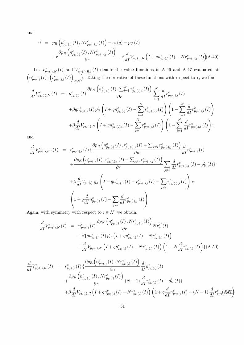
and
0 = pR
(ne
pU (.) (I) , NrepU (.),j (I)
)− cr (q) − pU (I)
+r∂pR
(ne
pU (.) (I) , NrepU (.),j (I)
)
∂r− β
d
dIVpU (.),R
(I + qne
pU (.) (I) − NrepU (.),j (I)
)(A-49)
Let V epU (.),N (I) and V e
pU (.),R,i (I) denote the value functions in A-46 and A-47 evaluated at(ne
pU (.) (I) ,(repU (.),i (I)
)
i∈N
). Taking the derivative of these functions with respect to I, we find
d
dIV e
pU (.),N (I) = nepU (.) (I)
∂pN
(ne
pU (.) (I) ,∑N
i=1 repU (.),i (I)
)
∂r
N∑
i=1
d
dIrepU (.),i (I)
+βqnepU (.) (I) p′U
(I + qne
pU (.) (I) −N∑
i=1
repU (.),i (I)
)(1 −
N∑
i=1
d
dIrepU (.),i (I)
)
+βd
dIVpU (.),N
(I + qne
pU (.),i (I) −N∑
i=1
repU (.),i (I)
)(1 −
N∑
i=1
d
dIrepU (.),i (I)
);
and
d
dIV e
pU (.),R,i (I) = repU (.),i (I)
∂pR
(ne
pU (.) (I) , repU (.),i (I) +
∑j 6=i r
epU (.),j (I)
)
∂n
d
dIne
pU (.) (I)
+∂pR
(ne
pU (.) (I) , repU (.),i (I) +
∑j 6=i r
epU (.),j (I)
)
∂r
∑
j 6=i
d
dIrepU (.),j (I) − p′U (I)
+βd
dIVpU (.),R,i
I + qne
pU (.) (I) − repU (.),i (I) −
∑
j 6=i
repU (.),j (I)
∗
1 + q
d
dIne
pU (.) (I) −∑
j 6=i
d
dIrepU (.),j (I)
Again, with symmetry with respect to i ∈ N , we obtain:
d
dIV e
pU (.),N (I) = nepU (.) (I)
∂pN
(ne
pU (.) (I) , NrepU (.) (I)
)
∂rNre
p′ (I)
+βqnepU (.) (I) p′U
(I + qne
pU (.) (I) − NrepU (.) (I)
)
+d
dIVpU (.),N
(I + qne
pU (.) (I) − NrepU (.) (I)
)(1 − N
d
dIrepU (.) (I)
)(A-50)
d
dIV e
pU (.),R (I) = repU (.) (I)
∂pR
(ne
pU (.) (I) , NrepU (.) (I)
)
∂n
d
dIne
pU (.) (I)
+∂pR
(ne
pU (.) (I) , NrepU (.) (I)
)
∂r(N − 1)
d
dIrepU (.) (I) − p′U (I)
+βd
dIVpU (.),R
(I + qne
pU (.) (I) − NrepU (.) (I)
)(1 + q
d
dIne
pU (.) (I) − (N − 1)d
dIrepU (.) (I)
)(A-51)
51

We thus have four equations (A-46), (A-47), (A-50) and (A-51) determining the four unknowns
nepU (.) (I), re
pU (.) (I), ddI V e
N (I) and ddI V e
R (I), for a given pU (I).
Step 2: Equilibrium peU (I).
As mentioned above, the ‘market clearing’ price, peU (I) is such that the obtained Cournot
equilibrium satisfies Nrepe
U(.) (I) = I for pe
U (.) > 0, or Nrepe
U(.) (I) < I for pe
U (.) = 0. Let (ne(I), re(I))
denote (nepU (.) (I) , re
pU (.) (I)) and (V e′R (I) , V e′
N (I)) denote(
ddI V e
peU
(.),R (I) , ddI V e
peU
(.),N (I)).
Consider peU (I) > 0 and Nre (I) = I. Substituting these in (A-46), (A-47), (A-50) and (A-51),
we obtain:
pN (ne(I), I) − cn (q) + βqpeU (qne(I)) + ne(I)
(∂pN (ne(I),I)
∂n + βq2pe′U (qne(I))
)+ βqV e′
N (qne(I)) = 0
pR (ne(I), I) − cr (q) − peU (I) + I
N∂pR(ne(I),I)
∂r − βV e′R (qne(I)) = 0
V e′N (I) = ne(I)∂pN (ne(I),I)
∂r
V e′R (I) = I
N
(∂pR(ne(I),I)
∂n ne′(I) + ∂pR(ne(I),I)∂r
N−1N − pe′
U (I))
+ βV e′R (qne(I))
(1N + qne′(I)
)
(A-52)
The solution to this set of four equations determines the four unknowns ne (I) , peU (I), V e′
N (I) and
V e′R (I). In the next step, we study the case of I = 0 and q = 0. Under these conditions, we have
that∑N
i=1 rei (0) = 0. We will use (A-52), and validate that pe
U (0) > 0.
Step 3: Derivative of V eN (I, q) with respect to q evaluated at q = 0.
In this step, we reintroduce the dependence of all previous expressions with respect to q. Taking
the partial derivative of V eN (I, q) with respect to q yields
∂V eN (I, q)
∂q= ne (I)
(−c′n (q) + βpe
U (qne (I)) + βqne (I) pe′U (qne (I))
)
+βne (I)∂V e
N (I + qne (I) − Nre (I) , q)
∂I+ β
∂V eN (I + qne (I) − Nre (I) , q)
∂q.
Evaluated for I = 0 and q = 0, can write the previous expression as
(1 − β)∂V e
N (0, 0)
∂q= ne(0)
(βpe
U (0) − c′n (q))
+ βne(0)∂V e
N (0, 0)
∂I. (A-53)
Substituting I = 0 and q = 0 in the first equation of (A-52), we obtain pN (ne(0), 0) − cn (0) +
ne(0)∂pN (ne(0),0)∂n = 0, which can be rewritten as ∂R(ne(0),0)
∂n = cn (0), and is solved by nsu (see
definition of nsu). Substituting I = 0 and q = 0 in the fourth equation of (A-52), we obtain
V e′R (0) = βV e′
R (0) 1N , from which it follows that V e′
R (0) = 0. Plugging the latter result in the
second equation of (A-52), we obtain pR (nsu, 0) − cr (0) = peU (0).
Using the proof of Lemma 4, we see that pR (nsu, 0) = (1 − δ) pN (nsu, 0) and that pN (nsu, 0) >∂R(nsu,0)
∂n . Therefore, peU (0) = (1 − δ) pN (nsu, 0)−cr (0) > (1 − δ) ∂R(nsu,0)
∂n −cr (0) = (1 − δ) cn (0)−cr (0). Thus, if (1 − δ) cn (0) > cr (0), then pe
U (0) > 0, which validates our assumption in step 2.
52
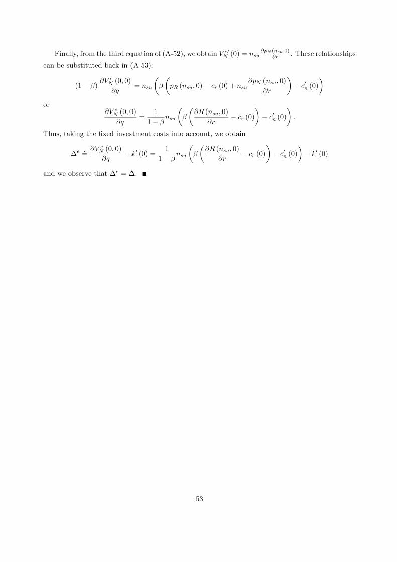
Finally, from the third equation of (A-52), we obtain V e′N (0) = nsu
∂pN (nsu,0)∂r . These relationships
can be substituted back in (A-53):
(1 − β)∂V e
N (0, 0)
∂q= nsu
(β
(pR (nsu, 0) − cr (0) + nsu
∂pN (nsu, 0)
∂r
)− c′n (0)
)
or∂V e
N (0, 0)
∂q=
1
1 − βnsu
(β
(∂R (nsu, 0)
∂r− cr (0)
)− c′n (0)
).
Thus, taking the fixed investment costs into account, we obtain
∆e .=
∂V eN (0, 0)
∂q− k′ (0) =
1
1 − βnsu
(β
(∂R (nsu, 0)
∂r− cr (0)
)− c′n (0)
)− k′ (0)
and we observe that ∆e = ∆.
53