Factors Affecting Product Supply in the Domestic Agrarian

http://rwe.sciedupress.com Research in World Economy Vol. 11, No. 5; Special Issue, 2020

Published by Sciedu Press 246 ISSN 1923-3981 E-ISSN 1923-399X

Factors Affecting Product Supply in the Domestic Agrarian Market in

Azerbaijan

Sugra Ingilab Humbatova1,2,3 & Natig Gadim-Oglu Hajiyev3,4

1 Department of Economy and Management, International Center for Graduate Education, Azerbaijan State

University of Economics (UNEC), Baku, Azerbaijan

2 Department of World Economy, Baku Engineering University (BEU), Khirdalan, Absheron, Azerbaijan

3 Ministry of Agriculture of Azerbaijan, Agrarian Science and Innovation Center, Azerbaijan

4 Department of Regulation of Economy, Azerbaijan State University of Economics (UNEC), Baku, Azerbaijan

Correspondence: Natig Gadim-Oglu Hajiyev, Istiqlaliyyat Str. 6, Baku, AZ-1001, Azerbaijan.

Received: July 1, 2020 Accepted: August 14, 2020 Online Published: September 3, 2020

doi:10.5430/rwe.v11n5p246 URL: https://doi.org/10.5430/rwe.v11n5p246

Abstract

The purpose of the study was to study, analyze, evaluate and forecast the factors affecting the formation of product

supply in the domestic agrarian market. Socio-economic aspects of the factors influencing the growth of product

supply in agrarian market in the country were considered for the purpose of the research. Statistical and econometric

analysis was carried out by the method of generalization, grouping, systematic approach, the role and place of factors

influencing the growth of product supply in agrarian market. The methodology used is based on econometric analysis

of time series. The first step involves the formation of an order of integration of variables included in the model and

utilizing several unit root tests such as the Augmented Dickey-Fuller (ADF), Phillips-Perron (PP) and

Kwiatkowski-Phillips-Schmidt-Shin (KPSS) tests. The cointegration approach is based on the ARDL model and the

boundary test. The relative volatility of some indicators, which indirectly depends on oil prices, has led to some

limitations in the study. The originality of the research is a complex statistical and econometric analysis of the factors

influencing the increase of product supply in the domestic agricultural market, and the scientific novelty is the

determination of the dependence of product supply in the agricultural sector on government support, including

investment. The application of the article in the development of this section on the impact of agricultural supply on

food security is of practical importance.

Keywords: agriculture, agrarian market, econometric analysis, product supply, government support

1. Introduction

The situation in the agricultural sector affects the socio–economic development of the whole economy. The specific

role assigned to the agricultural sector is conditioned, on the one hand, by the production of food products as a basis

for the reproduction of human life and labor, and, on the other hand, by the production of raw materials for other

industries. In other words, in essence, the development of the agricultural sector determines the level of economic

security of the country, including food security. Today, the development of the agrarian sector is one of the main

priorities of the state's socio–economic and agrarian policy. When analyzing and solving the problem of development

of the agrarian sector and the formation and increase of product supply in the agrarian market, it is necessary to study

them comprehensively with the solution of the problems of food security, employment in agriculture, increase of

incomes of those engaged in agrarian production.

2. Literature Review

In recent decades, the potential contribution of agriculture to economic growth has been the subject of great

controversy among representatives of developing economies (Titus, 2009). Some scholars argue that economic

growth depends on the development of the agricultural sector (Schultz, 2002). Proponents argue that investment in

agriculture is accompanied by the creation of institutions and infrastructure in other sectors, which is the basis for

national economic growth (Timmer, 1995; Timmer,2002; Gardner et al., 2001). Researchers have noted that growth

in the agricultural sector can play a catalytic role through resource conditions for the transition to rural incomes and

the industrial economy (Eicher and Staatz, 1990; Dowrick and Gemmell, 1991; Datt and Ravallion, 1998; Thirtle et



al., 2003). The focus of many developing countries on industrial development before the agricultural sector has led to

some contrasts in economic growth and excessive differences in income distribution. Others have shown that there is

a positive link between agriculture and economic growth, and that agriculture has an impact on economic growth

(Wang et al., 2010).

Many scientists have turned to econometrics in their research in this area. For example, an econometric analysis of

the relationship between the agricultural, industrial, and service sectors to GDP growth (Mirza and Moyen, 2015)

concludes that any change in agricultural sector strategy will affect the economy and the majority of the population

(Alam, 2008). In addition, the relationship between the agricultural production, services and trade sectors in Poland

and Romania was analyzed using the complex regression equation of the impact of agriculture on GDP in China and

the three African Sahara (SSA) countries (Andzio–Bika et al., 2004). evaluated by econometric model (Subramaniam

and Reed.2009).

Conducted an econometric analysis of the relationship between per capita income, agriculture and manufacturing

sectors in India (Singapore, 2015), empirical analysis of Nigeria's contribution to economic growth in agriculture

(Tolulope and Chinonso, 2013), Nigeria's contribution to economic growth in agricultural credit (Anthony, 2010),

Inter–sectoral adjustment and economic growth in Saudi Arabia have been analyzed as a basis for a successful long–

term development strategy (Abdulkarim et al., 2014).

3. Methodology and Methods

The data were obtained from the State Statistics Committee of Azerbaijan.

Table 1. Data and internet resource

Melon products MP www.stat.gov.az

Production of cereals and legumes PCL www.stat.gov.az

Harvesting of autumn wheat HAW www.stat.gov.az

Collection of potatoes CP www.stat.gov.az

Harvesting of vegetables HV www.stat.gov.az

Harvesting of fruits and berries HFB www.stat.gov.az

Harvesting of grapes HG www.stat.gov.az

Harvesting of sugar beet HSB www.stat.gov.az

Meat production MtP www.stat.gov.az

Milk production MkP www.stat.gov.az

Egg production WP www.stat.gov.az

Bovine cattle BC www.stat.gov.az

Sheep and goats SG www.stat.gov.az

Birds B www.stat.gov.az

Planting area PA www.stat.gov.az

Technique Park TP www.stat.gov.az

Agricultural workers AW www.stat.gov.az

Import of agricultural machinery for land IAML www.stat.gov.az

Import of equipment for processing of agricultural products IEPAP www.stat.gov.az

Import of equipment for the food industry IEFI www.stat.gov.az

3.1 Methodology

The supply of products in the agricultural market includes many agricultural products in all categories of production:

production of cereals and legumes, total harvest of winter wheat, potatoes, vegetables, fruits and berries, grapes, sugar

beets, meat, milk and eggs, including The main factors influencing the dynamics of the economy, including GDP and

gross agricultural output by all categories of farms, are the number of cattle, sheep and goats, birds in all categories,

agricultural machinery for cultivation, cultivation of agricultural crops. areas, agriculture, forestry and fisheries

investment, the fleet of major types of agricultural machinery, the number of employees in agriculture, forestry and



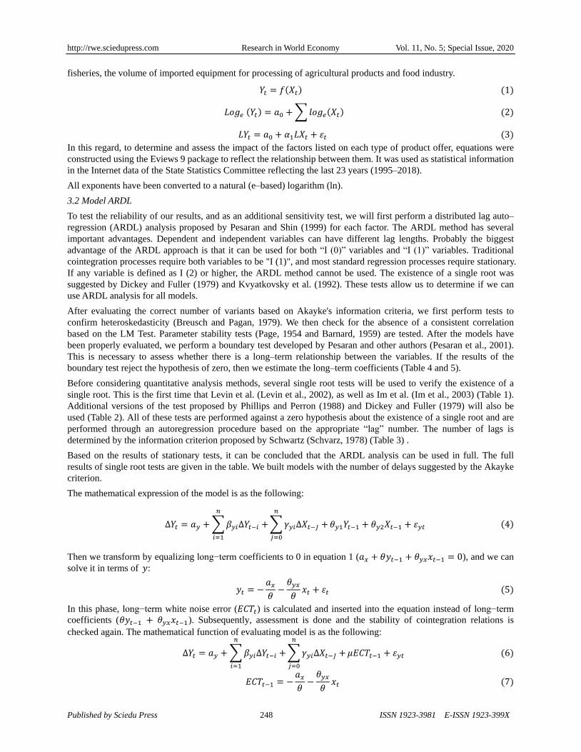
fisheries, the volume of imported equipment for processing of agricultural products and food industry.

𝑌𝑡 = 𝑓(𝑋𝑡) (1)

𝐿𝑜𝑔𝑒 (𝑌𝑡) = 𝑎0 +∑𝑙𝑜𝑔𝑒(𝑋𝑡) (2)

𝐿𝑌𝑡 = 𝑎0 + 𝛼1𝐿𝑋𝑡 + 𝜀𝑡 (3)

In this regard, to determine and assess the impact of the factors listed on each type of product offer, equations were

constructed using the Eviews 9 package to reflect the relationship between them. It was used as statistical information

in the Internet data of the State Statistics Committee reflecting the last 23 years (1995–2018).

All exponents have been converted to a natural (e–based) logarithm (ln).

3.2 Model ARDL

To test the reliability of our results, and as an additional sensitivity test, we will first perform a distributed lag auto–

regression (ARDL) analysis proposed by Pesaran and Shin (1999) for each factor. The ARDL method has several

important advantages. Dependent and independent variables can have different lag lengths. Probably the biggest

advantage of the ARDL approach is that it can be used for both “I (0)” variables and “I (1)” variables. Traditional

cointegration processes require both variables to be "I (1)", and most standard regression processes require stationary.

If any variable is defined as I (2) or higher, the ARDL method cannot be used. The existence of a single root was

suggested by Dickey and Fuller (1979) and Kvyatkovsky et al. (1992). These tests allow us to determine if we can

use ARDL analysis for all models.

After evaluating the correct number of variants based on Akayke's information criteria, we first perform tests to

confirm heteroskedasticity (Breusch and Pagan, 1979). We then check for the absence of a consistent correlation

based on the LM Test. Parameter stability tests (Page, 1954 and Barnard, 1959) are tested. After the models have

been properly evaluated, we perform a boundary test developed by Pesaran and other authors (Pesaran et al., 2001).

This is necessary to assess whether there is a long–term relationship between the variables. If the results of the

boundary test reject the hypothesis of zero, then we estimate the long–term coefficients (Table 4 and 5).

Before considering quantitative analysis methods, several single root tests will be used to verify the existence of a

single root. This is the first time that Levin et al. (Levin et al., 2002), as well as Im et al. (Im et al., 2003) (Table 1).

Additional versions of the test proposed by Phillips and Perron (1988) and Dickey and Fuller (1979) will also be

used (Table 2). All of these tests are performed against a zero hypothesis about the existence of a single root and are

performed through an autoregression procedure based on the appropriate “lag” number. The number of lags is

determined by the information criterion proposed by Schwartz (Schvarz, 1978) (Table 3) .

Based on the results of stationary tests, it can be concluded that the ARDL analysis can be used in full. The full

results of single root tests are given in the table. We built models with the number of delays suggested by the Akayke

criterion.

The mathematical expression of the model is as the following:

𝑌𝑡 = 𝑎 +∑ 𝑌𝑡 +

1

∑ 𝑋𝑡 +

0

1𝑌𝑡 1 + 2𝑋𝑡 1 + 𝜀 𝑡 (4)

Then we transform by equalizing long−term coefficients to 0 in equation 1 (𝑎 + 𝑡 1 + 𝑡 1 = ), and we can

solve it in terms of :

𝑡 = 𝑎 𝑡 + 𝜀𝑡 (5)

In this phase, long−term white noise error ( 𝑡) is calculated and inserted into the equation instead of long−term

coefficients ( 𝑡 1 + 𝑡 1). Subsequently, assessment is done and the stability of cointegration relations is

checked again. The mathematical function of evaluating model is as the following:

𝑌𝑡 = 𝑎 +∑ 𝑌𝑡 +

1

∑ 𝑋𝑡 +

0

𝑡 1 + 𝜀 𝑡 (6)

𝑡 1 = 𝑎 𝑡 (7)



So, 𝑡 or 𝑡 is true value of dependent variable. (

𝑡) is calculated value according to long−term equation

(equation 1). In equation 3, if is between 1 and and statistically important, then the cointegration realtions are

constant. Deviation for short term period is inclined to be corrected towards long term relation. In case any serious

calculation error is not noted, is getting close to coefficient in equation 1, sometimes gets equal value.

At the first phase, regression analysis for non−original stationary but the same−level differentiated stationary (I(1))

variables is assessed. So, for the case of two variables:

𝑡 = 𝛼0 + 𝛼1 𝑡 + 𝜀𝑡 (8)

Thus, 𝛼0 and 𝛼1 − regression coefficients, and – dependent and independent variables, 𝜀 – white noise error, – time. Having assessed regsression analysis, the next phase is to check whether 𝜀 is white noise error. If 𝜀𝑡 is

stationary, there will be cointegration relations among these variables. Accordingly, it will be considered as long−term

equations. At the last phase, ECM is assessed by using delayed white noise error (𝜀𝑡 1) and converting cause−effect

relations into stationary one.

𝑌𝑡 = 𝑎 +∑ 𝑌𝑡 +

1

∑ 𝑋𝑡 +

0

𝑡 1 + 𝜀 𝑡 (9)

Thus, 𝑎 , , coefficiants are mentioned. is a optimum delayed measure and 𝜀 is a white noise error of

the model. In case of having constant cointegration relations, Error Correction Term – ECT, thus 𝑡 1 coefficient

is negative and statistically important. Usually, this changes 1 and If it is greater than 1 this correction

process is going to be high.

4. Empirical Results

4.1 Results of Unit Root Tests

As mentioned earlier, we begin by testing the integration of different variables using ADF, PP, and KPSS tests. The

results of the three single root tests are given in Table 1 and Table 2. Approximately all three tests give the same

results, confirming the reliability of our results. We can assume that none of the variables are integrated into the

second level.

Table 1. Unit root tests Panel

Variable Levin, Lin and

Chu t

Im, Pesaran and

Schin W–stat

ADF–Fischer Chi

Square

PP–Fischer Chi

Square

Conclusion

LMP –5.87618*** –4.03569*** 69.6466*** 27.2097* I(0)

LPCL –5.51027*** –3.22822*** 62.4679*** 19.4140 I(1)

In first difference –11.2449*** –10.0091*** 102.774*** 114.758***

LHAW –5.72631*** –3.64076*** 65.5986*** 21.3751 I(1)


LCP –6.41613*** –4.59198*** 75.9687*** 32.1249** I(0)

LHV –5.48198*** –3.59204*** 65.1545*** 24.4587* I(0)

LHFB –5.26788*** –3.10996*** 61.9616*** 17.8688 I(1)


LHG –5.50569*** –3.70833*** 66.2244*** 20.2523 I(1)


LHSB –5.42467*** –3.30749*** 62.9427*** 19.0989 I(1)


LMtP –5.67425*** –4.35735*** 34.0310*** 77.3266*** I(0)

LMkP –2.43421** –1.28490 9.83982* 19.3031*** I(0)

LWP –3.84042*** –2.01582* 15.4843** 15.4009** I(0)

Note: values in the parenthesis represent the p value. * and ** indicate statistical significance at the respected

0.05 and 0.01 levels of significance.



Table 2. Unit Root Tests (ADF, PP, KPSS)

ADF Phillips–Perron KPSS

Level 1st difference Level 1st difference Level 1st difference

LMP Intercept –3.672634** –2.826665* –3.986381*** –2.779897* 0.525222** 0.494147** I(0)

Trend & Intercept –1.661652 –3.739991** –1.741905 –3.655090** 0.167639** 0.084111

None 1.713418 –2.668529** 1.263599 –2.591958**

LPCL Intercept –1.669227 –5.173644*** –1.983024 –6.238471*** 0.632894** 0.500000** I(1)

Trend & Intercept –2.367686 –4.721812*** –2.393640 –10.23087*** 0.163990** 0.500000***

None 1.492375 –4.763710*** 3.513391 –4.786334***

LHAW Intercept –2.692781* –4.537878*** –2.589663 –7.683177*** 0.579224** 0.500000** I(0)

Trend & Intercept –3.073752 –4.413949** –2.942564 –8.095731*** 0.126401* 0.500000**

None 0.695636 –4.568118*** 2.087992 –5.278137***

LCP Intercept –5.052829*** –1.583892 –5.052829*** –3.200009** 0.510241** 0.564407** I(0)

Trend & Intercept –2.065379 –4.754600*** –2.261149 –4.752371*** 0.184279** 0.145119*

None –0.240001** –2.118538** 1.499286 –3.030740***

LHV Intercept –4.142045*** –5.271260*** –3.363969** –5.142171*** 0.603988** 0.367830* I(0)

Trend & Intercept –3.223991 –3.950730** –2.135698 –5.178652*** 0.167128** 0.134206*

None 1.948755 –1.893647* 2.570608 –4.458042***

LHFB Intercept –1.412475 –7.426656*** –1.256485 –9.993472*** 0.698321** 0.251701 I(0)

Trend & Intercept –3.510947* –7.446849*** –3.510947* –17.50699*** 0.156314** 0.402438**

None 3.010484 –5.657066*** 4.423357 –5.591175***

LHG Intercept –2.259763 –3.429420** –2.261873 –3.356813** 0.160782 0.462268* I(0)

Trend & Intercept –4.785879*** –4.316617** –2.960291 –4.377748** 0.148096** 0.171902**

None –0.808248 –3.496559*** –0.694555 –3.425024***

LHSB Intercept –1.865900 –4.918137*** –1.865900 –4.915771*** 0.540506** 0.101148 I(1)

Trend & Intercept –2.203451 –4.826083*** –2.253532 –4.824879*** 0.128110* 0.048218

None 0.655944 –4.886455*** 0.710225 –4.886455***

LMtP Intercept –3.153891** –3.179911** –8.982006*** –3.043430** 0.706960** 0.505161** I(0)

Trend & Intercept –1.790276 –4.175078** –1.938488 –4.287385** 0.179437** 0.191809**

None 8.096754 –1.696549* 6.549402 –1.286720

LMkP Intercept –0.933688 –3.797633*** –0.933688 –3.797633*** 0.706708** 0.144888 I(0)

Trend & Intercept –3.508246* –4.032167** –1.522557 –4.032167** 0.064590 0.093693

None 12.84266 –1.152463 12.84266 –0.648381

LWP Intercept –0.579388 –4.512587*** –0.400480 –5.945121*** 0.694680** 0.267084 I(0)

Trend & Intercept –3.770215** –4.341819** –2.626947 –5.713731*** 0.102925 0.265775***

None 2.727636 –3.496253 5.902792 –3.469321***

LBC Intercept –3.787048*** 3.163740 –5.826452*** –0.276897 0.674576** 0.661100** I(0)

Trend & Intercept 1.904157 –5.809286*** 5.049311 –5.642330*** 0.193263** 0.131984*

None –3.336230*** –1.165348 3.680886 –1.084073

LSG Intercept –4.676262*** –0.637542 –4.173382*** –0.704705 0.643082** 0.593403** I(0)

Trend & Intercept –0.432821 –3.366218* 0.998314 –4.685849*** 0.190570** 0.127772*

None 0.060277 –0.862921 2.843871 –0.820877

LB Intercept –5.052829*** –1.583892 –5.052829*** –3.200009** 0.510241** 0.564407** I(0)

Trend & Intercept –2.065379 –4.754600*** –2.261149 –4.752371*** 0.184279** 0.145119**

None –0.240001 –2.118538** 1.499286 –3.030740***

LPA Intercept –0.469814 –4.247930*** –0.559355 –4.234967*** 0.605123** 0.152014 I(1)

Trend & Intercept –2.795675 –4.341401** –2.699713 –4.391597** 0.078160 0.097288

None 0.962586 –4.175466*** 1.085959 –4.160613**

LTP Intercept –2.111025 –3.930289*** –2.138881 –3.930868*** 0.473754** 0.185176 I(1)

Trend & Intercept –1.726842 –4.107091*** –1.862931 –4.057927** 0.141264* 0.063890

None –0.321736 –4.039617*** –0.328185 –4.040257***

LAW Intercept 0.792477 –6.918204*** 0.792477 –6.918204*** 0.669293** 0.479422** I(1)

Trend & Intercept –3.128392 –7.724645*** –3.168316 –9.519979*** 0.171378** 0.090568

None 2.060966 –5.130067*** 2.457790 –5.086439***

LIAML Intercept –2.190783 –5.568428*** –2.917890* –5.667217*** 0.679513** 0.500000** I(0)



Trend & Intercept –3.986444** –6.839234*** –3.236761 –10.16664*** 0.144527* 0.500000***

None 0.915576 –4.254482*** 1.405578 –4.714391***

LIEPAP Intercept –11.12009*** –4.638987*** –2.715192* –4.638987*** 0.574978** 0.282622 I(0)

Trend & Intercept –6.278620*** –5.656698*** –1.464107 –6.489772*** 0.171095** 0.140342*

None 0.987038 –4.273847*** 0.987038 –4.272079***

LIEFI Intercept –2.287770 –3.837543*** –2.214773 –5.691819*** 0.454186* 0.256797 I(1)

Trend & Intercept –2.490288 –4.026699** –2.509444 –7.318474*** 0.156570** 0.180017**

None 0.389327 –5.261758*** 0.961876 –5.631332***

Note: values in the parenthesis represent the p value. *, ** and *** indicate statistical significance at the

respected 0.1, 0.05, and 0.01 levels of significance.

4.2 VAR Lag Order Selection Criteria

In order to determine optimal lag for ARDL model, VAR Lag Order Selection Criteria was employed and we got the

below−mentioned results (Table 3).

According to Table 3, optimum lag period for all models is 1 (lag=1) based on 2 accepted information criteria (AIC and

SC).

Table 3. VAR Lag order selection criteria

Lag LogL LR FPE AIC SC HQ

LMP 1 98.70357 176.4856* 7.11e–11* –3.713354* –0.948672* –3.018044*

LPCL 1 90.67892 148.2528* 1.43e–10* –3.015558* –0.250877* –2.320249*

LHAW 1 94.05860 150.2221* 1.07e–10* –3.309443* –0.544762* –2.614134*

LCP 1 98.01940 155.7278* 7.55e–11* –3.653861* –0.889179* –2.958551*

LHV 1 98.59811 145.1637* 7.18e–11* –3.704183* –0.939502* –3.008874*

LHFB 1 112.7470 154.8050* 2.10e–11* –4.934518* –2.169836* –4.239208*

LHG 1 81.87888 159.1856* 3.07e–10* –2.250337* 0.514344* –1.555028*

LHSB 1 64.46104 140.0340* 1.40e–09* –0.735743* 2.028939* –0.040433*

LMtP 1 253.9867 201.7985* 1.76e–14* –20.34667* –19.35929* –20.09835*

LMkP 1 148.8730 191.8811* 7.87e–09* –12.98845* –12.69090* –12.91836*

LWP 1 45.34422 107.6644* 9.62e–05* –3.576748* –3.279191* –3.506652*

* indicates lag order selected by the criterion

LR: sequential modified LR test statistic (each test at 5% level)

FPE: Final prediction error

AIC: Akaike information criterion

SC: Schwarz information criterion

HQ: Hannan–Quinn information criterion

Table 4. Bounds test

ARDL Bounds Test Null Hypothesis of No

Long–Run Relationship

ARDL(1,1,1,0,1,1,1) C @TREND1 3.448147 Failed to reject

ARDL(1, 0, 0, 1, 0)2 4.111522* Rejected

ARDL(1, 0, 0, 0, 0, 0, 0) 3 2.463027 Failed to reject

ARDL(1, 0, 1, 0, 0, 0, 0) 3 4.540147*** Rejected

ARDL(1, 1, 1, 1, 1, 1) 4 2.198584 Failed to reject

ARDL(1, 1, 0, 1)6 3.689006 Failed to reject

ARDL(1, 1, 0, 1, 0, 1, 1) 2 3.466548 Failed to reject

ARDL(1, 0, 0, 0, 1, 0) 5 2.289684 Failed to reject

ARDL(1, 0, 1, 1)6 1.629670 Failed to reject

ARDL(1, 0)7 0.319185 Failed to reject



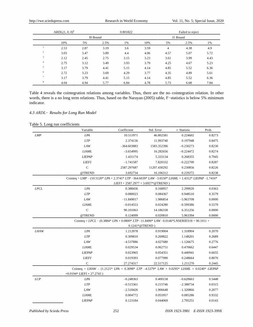
ARDL(1, 0, 0)8 0.801822 Failed to reject

I0 Bound I1 Bound

10% 5% 2.5% 1% 10% 5% 2.5% 1%

1 2.53 2.87 3.19 3.6 3.59 4 4.38 4.9 2 3.03 3.47 3.89 4.4 4.06 4.57 5.07 5.72 3 2.12 2.45 2.75 3.15 3.23 3.61 3.99 4.43 4 2.75 3.12 3.49 3.93 3.79 4.25 4.67 5.23 5 3.17 3.79 4.41 5.15 4.14 4.85 5.52 6.36 6 2.72 3.23 3.69 4.29 3.77 4.35 4.89 5.61 7 3.17 3.79 4.41 5.15 4.14 4.85 5.52 6.36 8 4.04 4.94 5.77 6.84 4.78 5.73 6.68 7.84

Table 4 reveals the cointegration relations among variables. Thus, there are the no–cointegration relation. In other

words, there is a no long term relations. Thus, based on the Narayan (2005) table, F−statistics is below 5% minimum

indicator.

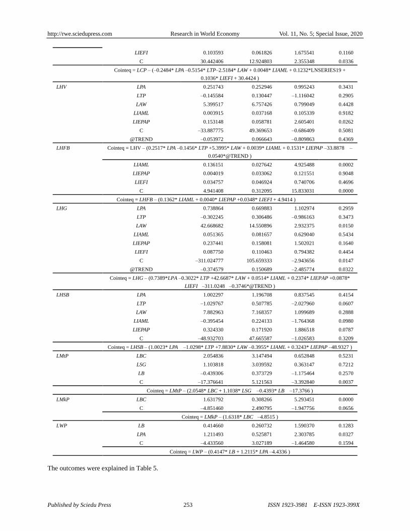
4.3 ARDL− Results for Long Run Model

Table 5. Long run coefficients

Variable Coefficient Std. Error t−Statistic Prob.

LMP LPA 10.511971 46.802581 0.224602 0.8273

LTP 2.374136 11.993740 0.197948 0.8475

LAW –364.603883 1583.352396 –0.230273 0.8230

LIAML –3.654995 16.282656 –0.224472 0.8274

LIEPAP 1.431174 5.333134 0.268355 0.7945

LIEFI –1.741587 7.820332 –0.222700 0.8287

C 2587.297687 11207.430292 0.230856 0.8226

@TREND 3.692734 16.106312 0.229272 0.8238

Cointeq = LMP – (10.5120* LPA + 2.3741* LTP –364.6039* LAW –3.6550* LIAML + 1.4312* LIEPAP –1.7416*

LIEFI + 2587.2977 + 3.6927*@TREND )

LPCL LPA 0.388436 0.168957 2.299020 0.0363

LTP 0.080023 0.084367 0.948510 0.3579

LAW –11.849017 1.986854 –5.963708 0.0000

LIAML –0.014553 0.024280 –0.599386 0.5579

C 90.101063 14.186338 6.351256 0.0000

@TREND 0.124099 0.020810 5.963394 0.0000

Cointeq = LPCL – (0.3884* LPA + 0.0800* LTP –11.8490* LAW –0.0146*LNSERIES18 + 90.1011 +

0.1241*@TREND )

LHAW LPA 1.212078 0.919004 1.318904 0.2070

LTP 0.309810 0.269822 1.148201 0.2689

LAW –4.537886 4.027680 –1.126675 0.2776

LIAML 0.029534 0.062751 0.470662 0.6447

LIEPAP 0.023965 0.054351 0.440941 0.6655

LIEFI 0.019393 0.077990 0.248664 0.8070

C 27.274317 22.517125 1.211270 0.2445

Cointeq = LHAW – (1.2121* LPA + 0.3098* LTP –4.5379* LAW + 0.0295* LIAML + 0.0240* LIEPAP

+0.0194* LIEFI + 27.2743 )

LCP LPA –0.248363 0.400158 –0.620663 0.5448

LTP –0.515361 0.215746 –2.388734 0.0315

LAW –2.518426 1.906648 –1.320866 0.2077

LIAML 0.004772 0.055957 0.085286 0.9332

LIEPAP 0.123184 0.044069 2.795251 0.0143



LIEFI 0.103593 0.061826 1.675541 0.1160

C 30.442406 12.924803 2.355348 0.0336

Cointeq = LCP – (–0.2484* LPA –0.5154* LTP–2.5184* LAW + 0.0048* LIAML + 0.1232*LNSERIES19 +

0.1036* LIEFI + 30.4424 )

LHV LPA 0.251743 0.252946 0.995243 0.3431

LTP –0.145584 0.130447 –1.116042 0.2905

LAW 5.399517 6.757426 0.799049 0.4428

LIAML 0.003915 0.037168 0.105339 0.9182

LIEPAP 0.153148 0.058781 2.605401 0.0262

C –33.887775 49.369653 –0.686409 0.5081

@TREND –0.053972 0.066643 –0.809863 0.4369

LHFB Cointeq = LHV – (0.2517* LPA –0.1456* LTP +5.3995* LAW + 0.0039* LIAML + 0.1531* LIEPAP –33.8878 –

0.0540*@TREND )

LIAML 0.136151 0.027642 4.925488 0.0002

LIEPAP 0.004019 0.033062 0.121551 0.9048

LIEFI 0.034757 0.046924 0.740706 0.4696

C 4.941408 0.312095 15.833031 0.0000

Cointeq = LHFB – (0.1362* LIAML + 0.0040* LIEPAP +0.0348* LIEFI + 4.9414 )

LHG LPA 0.738864 0.669883 1.102974 0.2959

LTP –0.302245 0.306486 –0.986163 0.3473

LAW 42.668682 14.550896 2.932375 0.0150

LIAML 0.051365 0.081657 0.629040 0.5434

LIEPAP 0.237441 0.158081 1.502021 0.1640

LIEFI 0.087750 0.110463 0.794382 0.4454

C –311.024777 105.659333 –2.943656 0.0147

@TREND –0.374579 0.150689 –2.485774 0.0322

Cointeq = LHG – (0.7389*LPA –0.3022* LTP +42.6687* LAW + 0.0514* LIAML + 0.2374* LIEPAP +0.0878*

LIEFI –311.0248 –0.3746*@TREND )

LHSB LPA 1.002297 1.196708 0.837545 0.4154

LTP –1.029767 0.507785 –2.027960 0.0607

LAW 7.882963 7.168357 1.099689 0.2888

LIAML –0.395454 0.224133 –1.764368 0.0980

LIEPAP 0.324330 0.171920 1.886518 0.0787

C –48.932703 47.665587 –1.026583 0.3209

Cointeq = LHSB – (1.0023* LPA –1.0298* LTP +7.8830* LAW –0.3955* LIAML + 0.3243* LIEPAP –48.9327 )

LMtP LBC 2.054836 3.147494 0.652848 0.5231

LSG 1.103818 3.039592 0.363147 0.7212

LB –0.439306 0.373729 –1.175464 0.2570

C –17.376641 5.121563 –3.392840 0.0037

Cointeq = LMtP – (2.0548* LBC + 1.1038* LSG –0.4393* LB –17.3766 )

LMkP LBC 1.631792 0.308266 5.293451 0.0000

C –4.851460 2.490795 –1.947756 0.0656

Cointeq = LMkP – (1.6318* LBC –4.8515 )

LWP LB 0.414660 0.260732 1.590370 0.1283

LPA 1.211493 0.525871 2.303785 0.0327

C –4.433560 3.027189 –1.464580 0.1594

Cointeq = LWP – (0.4147* LB + 1.2115* LPA –4.4336 )

The outcomes were explained in Table 5.



4.4 ARDL Model. ARDL− Results Error Correction (Short Run) Model

Table 6. Coefficients ARDL model

Model 1 Model 2 Model 3 Model 4 Model 5 Model 6 Model 7 Model 8 Model 9 Model 10 Model 11

DMP (–1) –0.437344

MP 0.468559

DPCL (–1) –0.337866

PCL 0.504374

DLHAW(–1) –0.549072

LHAW 0.861523

DLCP(–1) –0.357183

LCP 0.445034

DLHV(–1) –0.163041

LHV 0.805676

DLHFB (–1) –0.274946

LHFB 0.424065

DLHG (–1) –0.659486

LHG –0.124458

DLHSB (–1) –0.849175

LHSB 1.082191

DLMtP (–1) –0.111604

LMtP 0.082670

DLMkP (–1) 0.164587

LMkP –0.009118

DLWP (–1) –0.043939

LWP 0.138804

DLBC 0.830547 0.109013

DLSG 0.402297

DLB 0.068482 0.196362

LBC 0.580681 –0.278581 0.000672

LSG 0.265494

LB –0.059995 0.026714

DLPA 0.594545 0.783195 0.044960 0.392275 0.415085 –0.750729 3.563394 0.272092

DLTP –0.066996 –0.208843 0.027866 –0.149153 –0.131104 0.451781 –2.003352

AW 2.581221 –1.363666 0.803528 2.774211 2.714445 –1.316579 40.46012

DLIAML –0.054175 0.040287 0.019236 0.049452 –0.017428 0.038012 –0.044960 –0.155800

DLIEPAP 0.114799 0.011786 0.079863 0.082827 0.032582 –0.108723 0.418113

DLIEFI –0.010697 0.031669 0.078288 0.415085 –0.063366 –0.140212 0.002853

LPA –0.815803 –0.431030 0.383223 –0.293663 –0.131104 –0.156860 1.312192 –0.230959

LTP 0.118491 0.228220 0.086748 0.133060 2.714445 –0.340704 1.674977

LAW 1.170691 0.935868 –1.889671 2.353774 –0.017428 –2.898081 –0.260007

LIAML 0.079012 –0.044057 0.006904 –0.072456 0.082827 –0.049923 0.104635 –0.180047

LIEPAP –0.227911 –0.013664 –0.045954 0.415085 –0.026900 0.005358 –0.219591

LIEFI –0.012153 –0.091187 –0.114110 2.80E–05 0.125274 0.000570

C –5.257942 –9.616749 5.692757 –17.48425 –4.582364 –2.005777 24.58894 –27.25057 –0.229272 0.087282 0.580227

The results of ARDL model coefficients (Table 6).



Table 7. Estimates of the correlation coefficients (long–term and short–term)

Model 1 Model 2 Model 3 Model 4 Model 5 Model 6 Model 7 Model 8 Model 9 Model 10 Model 11

DMP (–1) 0.835256

DPCL (–1) –0.089364

DLHAW(–1) 0.340866

DLCP(–1) 0.309127

DLHV(–1) –0.100540

DLHFB (–1) –0.289217

DLHG (–1) 0.245767

DLHSB 8(–1) 0.254903

DLMtP (–1) 0.028095

DLMkP (–1) 0.152961

DLWP (–1) –0.032334

DLBC –0.080204

DLSG 0.349820

DLB 0.070588 0.024456 0.097499

DLPA –0.178966 0.937083 0.369308 0.087747 0.207382 –0.202667 –0.311982 –0.089801 0.319188

DLTP –0.292370 –0.214101 0.059442 –0.174340 –0.060702 0.132118 –0.270396

DLAW 10.69479 –2.502179 –6.002750 0.820588 4.425060 4.880925 –3.742556 –0.625368

DLIAML 0.025156 0.034191 0.025874 0.006788 –0.010195 0.028884 –0.028801 0.034728

DLIEPAP 0.119206 –0.044324 0.102522 0.082063 0.017245 –0.084309 0.081158 –0.008268

DLIEFI 0.084189 0.043484 0.117222 –0.056691 –0.141276 0.008784 0.002541

ECT (–1) –0.697214 –0.496543 –0.689227 –0.620078 –0.193119 –0.524031 –0.557041 –0.931577 –0.284903 –0.006221 –0.205384

C –0.120952 0.037047 0.047544 –0.012666 –0.005897 0.049796 0.008864 0.050303 0.041405 0.032860 0.045709

The resuls of short−term and ECM model have been illustrated (Table 7).

On the other hand, etc. coefficient is negative in all cases. Although ECM coefficient factors are not important,

according to Pesaran and others (2001) they pave the way for having the cointegration relations because of negativity.

4.5 Diagnostic Test

Table 8. Diagnostic test results (F and LM Version)

Heteroskedasticity Test:

ARCH

Heteroskedasticity Test:

Breusch–Pagan–Godfrey

Breusch–Godfrey LM test

for serial correlation

Jarque–Bera

Probability

GUSUM /

GUSUM of

Squares F–Statistic Observed

R–Squared

F–Statistic Observed

R–Squared

F–Statistic Observed

R–Squared

LMP 0.689678

(0.4161)

0.733357

(0.3918)

0.542666

(0.8467)

10.10655

(0.6852)

0.420526

(0.6723)

2.467040

(0.2913)

4.373767

(0.112266)

stability/

stability

LPCL 0.402523

(0.5330)

0.434040

(0.5100)

0.605442

(0.7429)

5.066828

(0.6518)

1.202614

(0.3317)

3.591004

(0.1660)

1.347036

(0.509912)

stability/

stability

LHAW 0.652621

(0.4287)

0.695198

(0.4042)

0.341436

(0.9220)

3.161071

(0.8697)

1.865424

(0.1940)

5.128820

(0.0770)

0.096543

(0.952875)

stability/

stability

LCP 0.562288

(0.4621)

0.601603

(0.4380)

0.753968

(0.6466)

6.925513

(0.5447)

0.901402

(0.4318)

3.004063

(0.2227)

3.474044

(0.176044)

stability/

stability

LHV 0.082566

(0.7768)

0.090449

(0.7636)

2.205338

(0.1097)

16.69242

(0.1615)

1.937024

(0.2060)

7.504020

(0.0235)

0.957749

(0.619480)

stability/

stability

LHFB 3.716349

(0.0652)

3.198018

(0.0505)

1.615326

(0.2068)

8.676449

(0.1926)

0.615658

(0.5543)

1.859343

(0.3947)

0.950244

(0.621809)

stability/

stability

LHG 3.010162

(0.0981)

2.878014

(0.0898)

1.842642

(0.1705)

15.83750

(0.1988)

8.947005

(0.0091)

15.89411

(0.0004)

1.483988

(0.476164)

stability/

stability

LHSB 0.679472 0.722861 0.919705 6.907030 0.479179 1.579142 4.245980 stability/



(0.4195) (0.3952) (0.5184) (0.4386) (0.6298) (0.4540) (0.119673) no stability

LMtP 1.128286

(0.3008)

1.174837

(0.2784)

1.119387

(0.3944)

6.800193

(0.3397)

3.060068

(0.0790)

6.996132

(0.0303)

0.857478

(0.651330)

stability/

no stability

LMkP 0.962387

(0.3383)

1.010024

(0.3149)

0.017797

(0.9824)

0.040861

(0.9798)

0.264201

(0.7707)

0.655926

(0.7704)

1.373572

(0.503191)

stability/

no stability

LWP 0.955526

(0.3400)

1.003151

(0.3165)

1.651524

(0.2111)

4.757135

(0.1905)

1.523206

(0.2463)

3.495262

(0.1742)

1.619058

(0.445068)

stability/

stability

Regression equations are adequate. It also passes all the diagnostic tests against serial correlation (Durbin Watson test

and Breusch−Godfrey test), heteroscedasticity (White Heteroskedasticity Test), and normality of errors (Jarque−Bera

test). The Ramsey RESET test also suggests that the model is well specified. All the results of these tests are shown in

Table 8. The stability of the long−run coefficient is tested by the short−run dynamics. Once the ECM model has been

estimated, the cumulative sum of recursive residuals (CUSUM) and the CUSUM of square (CUSUMSQ) tests are

applied to assess the parameter stability (Pesaran and Pesaran, 1997). The results indicate the absence of any instability

of the coefficients because the plot of the CUSUM and CUSUMSQ statistic fall inside the critical bands of the 5%

confidence interval of parameter stability.

5. Conclusıon

The results of the study show that the gross agricultural output and gross agricultural output, the production of cereals

and legumes, winter wheat, potatoes, vegetables, fruits and berries, grapes, sugar beets, meat, milk and eggs The

number of people working in agriculture, forestry and fisheries, the number of cattle, sheep and goats, the number of

agricultural machinery, as well as the number of agricultural machinery for land cultivation, agriculture, forestry and

fisheries investment Intensive factors, such as the fleet of basic agricultural machinery, the processing of agricultural

products and the import of equipment for the food industry, also need to be addressed.

References

Abdulkarim, A. K., Al–shihri, F. S., & Ahmed, S. M. (2014). Inter–Sectoral Linkages and Economic Growth in Saudi

Arabia: Toward a Successful Long–term Development Strategy. International Journal of Science and Research

3(8), 1654-1659. Retrieved from https://www.ijsr.net/archive/v3i8/MDIwMTU3ODk=.pdf

Alam, G. (2008). The role of technical and vocational education in the national development of Bangladesh.

International Journal of Work–Integrated Learning, 9(1), 25. Retrieved from

https://www.ijwil.org/files/APJCE_09_1_25_44.pdf

Anthony, E. (2010). Agricultural credit and economic growth in Nigeria: An empirical analysis. Business and

Economics Journal, 14(1), 1-7.

Barnard, G. A. (1959). Control charts and stochastic processes. Journal of the Royal Statistical Society: Series B

(Methodological), 21(2), 239-257. https://doi.org/10.1111/j.2517-6161.1959.tb00336.x

Breusch, T. S., & Pagan, A. R. (1979). A simple test for heteroscedasticity and random coefficient variation.

Econometrica: Journal of the Econometric Society, 1287-1294. https://doi.org/10.2307/1911963

Datt, G., & Ravallion, M. (1998). Farm productivity and rural poverty in India. The Journal of Development Studies,

34(4), 62-85. https://doi.org/10.1080/00220389808422529

Dickey, D. A., & Fuller, W. A. (1979). Distribution of the estimators for autoregressive time series with a unit root.

Journal of the American Statistical Association, 74(366a), 427-431.

https://doi.org/10.1080/01621459.1979.10482531

Dowrick, S., & Gemmell, N. (1991). Industrialisation, catching up and economic growth: a comparative study across

the world's capitalist economies. The Economic Journal, 101(405), 263-275. https://doi.org/10.2307/2233817

Eicher, C. K. (1990). Agricultural development in the Third World, edited by Carl K. Eicher & John M. Staatz. The

Johns Hopkins studies in development. Retrieved from https://ru.booksc.xyz/book/50056655/d86841

Gardner, B. L., Rausser, G. C., Pingali, P. L., & Evenson, R. E. (Eds.) (2001). Handbook of Agricultural Economics:

Agriculture and Its External Linkages (Vol. 2). Elsevier.

Gollin, D., Parente, S. L., & Rogerson, R. (2002). The role of agriculture in development. American Economic Review,

https://www.ijsr.net/archive/v3i8/MDIwMTU3ODk=.pdf

https://www.ijwil.org/files/APJCE_09_1_25_44.pdf

https://ru.booksc.xyz/book/50056655/d86841



92(2), 160-164. https://doi.org/10.1257/000282802320189177

Im, K. S., Pesaran, M. H., & Shin, Y. (2003). Testing for unit roots in heterogeneous panels. Journal of Econometrics,

115(1), 53-77.

Kwiatkowski, D., Phillips, P. C., Schmidt, P., & Shin, Y. (1992). Testing the null hypothesis of stationarity against the

alternative of a unit root root: How sure are we that economic time series have a unit root?. Journal of

Econometrics, 54(1–3), 159-178. https://doi.org/10.1016/0304-4076(92)90104-Y

Levin, A., Lin, C. F., & Chu, C. S. J. (2002). Unit root tests in panel data: asymptotic and finite–sample properties.

Journal of Econometrics, 108(1), 1-24. https://doi.org/10.1016/S0304-4076(01)00098-7

MacKinnon, J. G. (1996). Numerical distribution functions for unit root and cointegration tests. Journal of Applied

Econometrics, 11(6), 601-618.

https://doi.org/10.1002/(SICI)1099-1255(199611)11:6<601::AID-JAE417>3.0.CO;2-T

Mirza Md. Moyen Uddin. (2015). Causal relationship between agriculture, industry and services sector for GDP

growth in Bangladesh: An econometric investigation. Journal of Poverty, Investment and Development, 8,

124-130. Retrieved from

http://citeseerx.ist.psu.edu/viewdoc/download?doi=10.1.1.676.6370&rep=rep1&type=pdf

Narayan, P. K. (2005). The saving and investment nexus for China: evidence from cointegration tests. Applied

Economics, 37(17), 1979-1990. https://doi.org/10.1080/00036840500278103

Page, E. S. (1954). Continuous inspection schemes. Biometrika, 41(1/2), 100-115.

https://doi.org/10.1093/biomet/41.1-2.100

Pesaran, M. H., & Shin, Y. (1999). An Autoregressive Distributed Lag Modelling Approach to Cointegration Analysis.

In S. Strom (Ed.), Econometrics and Economic Theory in the 20th Century: The Ragnar Frisch Centennial

Symposium (chp. 11). Cambridge: Cambridge University Press. Retrieved from


Pesaran, M. H., Shin, Y., & Smith, R. J. (2001). Bounds testing approaches to the analysis of level relationships.

Journal of Applied Econometrics, 16(3), 289-326. https://doi.org/10.1002/jae.616

Phillips, P. C., & Perron, P. (1988). Testing for a unit root in time series regression. Biometrika, 75(2), 335-346.

https://doi.org/10.1093/biomet/75.2.335

Schultz, T. W. (1964). Transforming traditional agriculture. Transforming traditional agriculture. Retrieved from

https://www.cabdirect.org/cabdirect/abstract/19641802933

Schwarz, G. (1978). Estimating the dimension of a model. The Annals of Statistics, 6(2), 461-464.

https://doi.org/10.1214/aos/1176344136

Singariya, M., & Sinha, N. (2015). Relationships among per capita GDP, agriculture and manufacturing sectors in

India. Journal of Finance and Economics, 3(2), 36-43.

Subramaniam, V., & Reed, M. R. (2009). Agricultural inter–sectoral linkages and its contribution to economic growth

in the transition countries (No. 1005–2016–79162). Contributed Paper Prepared for Presentation at the

International Association of Agricultural Economists Conference, Beijing, China, August 16-22.

Thirtle, C., Lin, L., & Piesse, J. (2003). The impact of research–led agricultural productivity growth on poverty

reduction in Africa, Asia and Latin America. World Development, 31(12), 1959-1985.

https://doi.org/10.1016/j.worlddev.2003.07.001

Timmer, C. P. (1995). Getting agriculture moving: do markets provide the right signals?. Food policy, 20(5), 455-482.

https://doi.org/10.1016/0306-9192(95)00038-G

Timmer, C. P. (2002). Agriculture and economic development. Handbook of Agricultural Economics, 2, 1487-1546.

https://doi.org/10.1016/S1574-0072(02)10011-9

Titus, O. A. (2009). Does agriculture really matter for economic growth in developing countries? (No. 319–2016–

9808). Selected Paper prepared for presentation at the American Agricultural Economics Association Annual

Meeting, Milwaukee, WI, July 28. Retrieved from




https://www.cabdirect.org/cabdirect/abstract/19641802933




Tolulope O., & Etumnu, C. (2013). Contribution of Agriculture to Economic Growth in Nigeria, The 18th Annual

Conference of the African Econometric Society (AES) Accra, Ghana at the session organized by the Association

for the Advancement of African Women Economists (AAAWE), 22nd and 23rd July. Retrieved from

https://pdfs.semanticscholar.org/1b7b/284b899d9cc59eba44c29fbc6db898946320.pdf

Wilfrid, A. B. H. L., & Edwige, K. (2004). Role of agriculture in economic development of developing countries: case

study of China and Sub–Saharan Africa (SSA). Journal of Agriculture and Social Research (JASR), 4(2), 1-18.

https://doi.org/10.4314/jasr.v4i2.2811

Notes

Note 1. This is an example.

Note 2. This is an example for note 2.

Copyrights

Copyright for this article is retained by the author(s), with first publication rights granted to the journal.

This is an open-access article distributed under the terms and conditions of the Creative Commons Attribution

license (http://creativecommons.org/licenses/by/4.0/).

https://pdfs.semanticscholar.org/1b7b/284b899d9cc59eba44c29fbc6db898946320.pdf

Documents

Factors Affecting Product Supply in the Domestic Agrarian