Embed Size (px)
Citation preview

I
Facial Pose Estimation and Face
Recognition from Three-
Dimensional Data
����������� � ����
����� ������������� �"!�#%$'&)(*�%�,+-&)./�0&�12 �034+5�6��78.9+;:�&<(>=?+5$A@91
2 � .�$'(?&)BC�
D #�EF#/=G$IH%J�J/K
D $'� &<=?+L=M! (?&)=,&).�$'&)NO$'� 2 ��34+P�Q��78.9+;:�&)(?=?+5$A@+L.R! BS(T$U+-BC���V#��6�W+5�Q�X�Y&).�$Z����$'� &[(?&)\�#�+-(>&<��&).�$'=��U� (I$'� &[N�&CE (?&)&[���
2 B�=G$'&)(?=+L.
���,+-&)./�0&
]_^-`�a?b-c/dfegaih�eFj�kSlGm�n opo�q

II
Abstract
Face recognition from 3D shape information has been proposed as a method of biometric
identification in recent times. This thesis presents a 3D face recognition system capable
of recognizing the identity of an individual from his/her 3D facial scan in any pose across
the view-sphere, by suitably comparing it with a set of models stored in a database. The
system makes use of only 3D shape information ignoring textural information
completely.
Firstly, the thesis proposes a generic learning strategy using support vector regression
[11] to estimate the approximate pose of a 3D scan. The support vector machine (SVM)
is trained on range images in several poses, belonging to a small set of individuals. This
thesis also examines the relationship between size of the range image and the accuracy of
the pose prediction from the scan.
Secondly, a hierarchical two-step strategy is proposed to normalize a facial scan to a
nearly frontal pose before performing recognition. The first step consists of a coarse
normalization making use of either the spatial relationships between salient facial
features or the generic learning algorithm using the SVM. This is followed by an iterative
technique to refine the alignment to the frontal pose, which is basically an improved form
of the Iterated Closest Point Algorithm [17]. The latter step produces a residual error
value, which can be used as a metric to gauge the similarity between two faces. Our two-
step approach is experimentally shown to outdo both the individual normalization
methods in terms of recognition rates, over a very wide range of facial poses. Our
strategy has been tested on a large database of 3D facial scans in which the training and
test images of each individual were acquired at significantly different times, unlike
several existing 3D face recognition methods.

III
Résumé
Récemment, la reconnaissance de visages avec de l’ information 3D a été proposé comme
une méthode d’authentification biométrique. Cette thèse décrit un système
d’ identification du visage 3D capable d’ identifier un individu de son balayage facial 3D
dans n’ importe quelle pose, à travers la sphère de vue, en le comparant à un ensemble de
modèles stockés dans une base de données. Le système emploie seulement l’ information
3D et ignore complètement la texture du visage.
D’abord, la thèse propose une stratégie générique d’apprentissage pour déterminer la
pose approximative d’un balayage 3D. La stratégie emploie un « Support Vector
Machine », qui est entraîné avec les images 3D appartenant à quelques individus dans
plusieurs poses. De même, la thèse examine le rapport entre l’exactitude d’estimation de
la pose et la taille de l’ image.
Deuxièmement, une technique hiérarchique de normalisation de pose est proposée pour
aligner un balayage facial sur une pose presque frontale, avant d’exécuter l’algorithme
d’ identification. La première étape consiste d’un alignement brut utilisant des rapports
spatiaux entre les saillants points du visage ou utilisant l’algorithme générique
d’apprentissage avec le « Support Vector Machine ». Ceci est suivi d’une méthode
itérative pour raffiner l’alignement. Cette étape est une forme améliorée de l’algorithme
« Iterated Closest Point » (ICP). La dernière étape produit une valeur d’erreur résiduelle
qui peut être employée comme une métrique pour quantifier la similitude entre deux
visages. Cette technique de normalisation en deux étapes est expérimentalement prouvée
de pouvoir surpasser les deux méthodes autonomes en termes de pourcentages
d’ identification obtenus, à travers plusieurs poses. Notre méthode à été examinée avec
une grande base de données, dans laquelle les images de formation et d’essai ont été
acquises à des heures différentes, contrairement aux systèmes existants d’ identification
du visage 3D.

IV
Acknowledgements First of all, I would like to thank my supervisor Professor Martin Levine for having
introduced me to such an exciting research topic, for his close guidance and
interactiveness throughout this thesis, and for his vast experience in the field of computer
vision. I would also like to thank my co-supervisor Professor Gregory Dudek for his
encouragement, cooperation and insightful comments.
This thesis is dedicated to my father Vilas, my mother Lalita and my younger brother
Varun. My parents have always shown me by way of example the meaning of thorough
professionalism, efficiency and cheerful spirit, in the face of all odds. The moral support
and encouragement given to me by my parents and brother is invaluable. For all this, I
shall always be grateful.
I would like to express my gratitude to several professors at McGill University, for
having shaped my understanding of the various aspects of computer vision: Prof. Doina
Precup and her student Bohdana Ratitch for artificial intelligence and probabilistic
reasoning, Prof. Michael Langer for computational perception, Prof. Martin Levine for
image processing, Prof. Stefan Langerman for computational geometry, Prof. Kaleem
Siddiqi for shape analysis and Prof. James Clark for statistical computer vision.
All through the course of the thesis, interactions with my friends have always proven
beneficial to me. Bhavin Shastri, Jisnu Bhattacharya, Gurman Singh Gill and Chris
(Yingfeng) Yu, thank you so much for your help and cooperation, and for so much fun!
And Ishana, thanks a lot for having helped me with the French abstract of the thesis. It
also gives me pleasure to take a sentence of appreciation for the ever-popular Gurman,
for having helped me in so many ways: for having shown me some fine details pertaining
to OpenGL, and for his friendly and thoughtful advice. His sense of humor has never
ceased to amaze me!

V
Table of Contents Abstract .......................................................................................................II
Résumé.......................................................................................................III
Acknowledgements.................................................................................... IV
List of Figures..........................................................................................VIII
List of Tables...............................................................................................X
Chapter One: Introduction............................................................................ 1
(1.1) Thesis Outline.................................................................................................3
(1.2) Contributions of the Thesis .............................................................................5
Chapter Two: Survey of 3D Face Recognition Techniques.......................... 7
(2.1) PCA Based Methods............................................................................................7
(2.2) Methods using Curvature.....................................................................................9
(2.3) Using Contours..................................................................................................11
(2.4) Methods Using Point Signatures........................................................................11
(2.5) Using Kimmel’s Eigenforms .............................................................................14
(2.6) Methods Based on Iterated Closest Point ...........................................................15
(2.7) Morphable Models.............................................................................................16
(2.8) Discussion.........................................................................................................19
(2.9) Overview of the Recognition Method Followed.................................................20
Chapter Three: Facial Pose Estimation .......................................................22
(3.1) Need for Facial Pose Estimation Techniques.................................................22
(3.2) Review of Existing Literature........................................................................23
(3.2.1) Feature-Based Methods..............................................................................23
(3.2.2) Appearance Based Methods.......................................................................24
(3.3) Approach Followed ...........................................................................................27
(3.4) Using Support Vector Regression......................................................................27
(3.4.1) Theory of Support Vector Regression ........................................................28

VI
(3.4.2) Motivation for using Support Vector Regression........................................30
(3.4.3) Experimental Setup....................................................................................31
(3.4.4) Use of Discrete Wavelet Transform ...........................................................31
(3.4.5) Sources of Data..........................................................................................32
(3.4.6) Pre-Processing of Data for Pose Estimation Experiments...........................34
(3.4.7) Training Using Support Vector Regression ................................................35
(3.4.8) Testing Using Support Vector Regression..................................................35
(3.5) Discriminant Isometric Mapping...................................................................43
(3.5.1) ISOMAP....................................................................................................43
(3.5.2) Discriminant ISOMAP...............................................................................44
(3.5.3) Motivation for Using Discriminant ISOMAP in Face Pose Estimation.......45
(3.5.4) Use of Discriminant Isometric Mapping for Pose Estimation .....................46
(3.5.5) Results with Discriminant ISOMAP...........................................................46
(3.6) Conclusions ..................................................................................................49
Chapter Four: 3D Face Recognition............................................................50
(4.1) Introduction.......................................................................................................50
(4.2) Feature-Based Method.......................................................................................51
(4.2.1) Facial Feature Detection ............................................................................51
(4.2.2) Facial Normalization and Recognition.........................................................53
(4.3) Results using the Feature-Based Method............................................................57
(4.4) Global Approach ...............................................................................................58
(4.4.1) Iterated Closest Point Algorithm..................................................................59
(4.4.2) Variant of ICP.............................................................................................60
(4.4.3) Improving Algorithm Speed ........................................................................62
(4.5) Experimental Results using the Global Approach ..............................................64
(4.5.1) Recognition Rate versus Pose......................................................................65
(4.5.2) The Two-step Cascade.................................................................................66
(4.5.3) Dealing with Missing Points........................................................................69
(4.5.4) Error Histograms.........................................................................................69
(4.5.5) Effect of Image Size on Recognition Rate..................................................71

VII
(4.5.6) Effect of Number of Gallery Images on Recognition Rate..........................71
(4.5.7) Implications for Expression Invariance........................................................72
(4.6) Conclusion ........................................................................................................75
Chapter Five: Conclusions and Future Work...............................................78
Citations .....................................................................................................83

VIII
List of Figures
Figure 1: Definition of Point Signature 13
Figure 2: Mean Face (Freiburg Database) 33
Figure 3:Sample Faces from the Freiburg Database 33
Figure 4: Faces from Notre Dame Database 33
Figure 5: Pose Estimation Accuracy versus Angular Sampling (Freiburg Database) 37
Figure 6: Error Histogram (Y-angle, Freiburg Database) 38
Figure 7: Error Histogram (X-angle, Freiburg Database) 39
Figure 8: Effect of Input Size on Accuracy of Estimation of Y-angle 41
Figure 9: Effect of Input Size on Accuracy of Estimation of X-angle 41
Figure 10:Pose Estimation Accuracy (Y-angle) vs. Number of Principal Components 42
Figure 11:Pose Estimation Accuracy (X-angle) vs. Number of Principal Components 42
Figure 12: Pose Estimation Accuracy (Y-angle) versus Number of neighbors (Freiburg Database)
48
Figure 13:Pose Estimation Accuracy (Y-angle) versus Number of neighbors (Notre Dame Database)
48
Figure 14:Depth Map 55
Figure 15: Red regions indicate concavities. Notice the two large concavities near the inner eye corners.
55
Figure 16: All Major Concave regions, each labeled with a different color 56
Figure 17: Distinct concavities: The blue and yellow regions represent the left and right inner eye concavities, respectively.
56
Figure 18: Face After Normalization 57
Figure 19: Face After Cropping 57
Figure 20: Cropped Models from the Notre Dame database 65
Figure 21: Cropped probe images from the Notre Dame database 65
Figure 22: Residual Error Histogram for images of the SAME people 70
Figure 23:Residual Error Values between different images of different persons 70
Figure 24: Residual Error Histogram for images of the SAME (left) and DIFFERENT (right) people shown together for comparison
71

IX
Figure 25: Recognition Rate versus Image Size 74
Figure 26: Recognition Rate versus Number of Training Images 74
Figure 27: Two scans of the same person with different facial expressions 75
Figure 28: Removal of non-rigid regions of the face (portions below the four dark lines)
75

X
List of Tables Table 1: Survey of Existing 3D Face Recognition Techniques
19
Table 2: Pose Estimation Results
38
Table 3: Recognition Rates with ICP, ICP Variant and LMICP
68
Table 4: Recognition Rates with ICP and the ICP Variants after applying the feature-based method as an initial step
68
Table 5: Recognition rates with ICP and ICP variant after applying SVR as the initial step
68

Chapter 1: Introduction ________________________________________________________________________
1
Chapter One: Introduction
Within the field of computer vision, a considerable amount of research has been
performed in recent times on automated methods for recognizing the identity of
individuals from their facial images. The major motivating factors for this are the
understanding of human perception, and a number of security and surveillance
applications such as access to ATMs, airport security, tracking of individuals and law-
enforcement. The human face remains one of the most popular cues for identity
recognition in biometrics, despite the existence of alternative technologies such as
fingerprint or iris recognition. The major reason for this is the non-intrusive nature of
face recognition methods, which makes them especially suitable to tracking applications.
Other biometric methods do not possess these advantages. For instance, iris recognition
methods require the users to place their eyes carefully relative to a camera [1]. Similarly,
fingerprint recognition methods require the users to make explicit physical contact with
the surface of a sensor [2].
Nevertheless, despite the above-mentioned advantages of face recognition as a method of
biometric identification, there are some issues that can seriously affect the performance
of a face recognition system. The appearance of the human face is subject to several
different changes owing to a combination of factors such as head pose, expressions,
illumination, occlusions, make-up and aging. To be of use in the real world, a face
recognition system should be robust to such changes. Traditionally, face recognition has
been performed using 2D images of a person, the reason being the cost-effectiveness and
easy availability of 2D sensors such as digital cameras. However, 2D face recognition
techniques are known to suffer from the above-mentioned drawbacks and are particularly
sensitive to changes in illumination [10]. In the recent past, increasingly cheaper and
advanced three-dimensional sensors have been released in the market [3]. Therefore, face
recognition from data obtained from three-dimensional scanners has been proposed as a
viable alternative to 2D methods. Three-dimensional scanners have the ability to capture
the complete geometry of a person’s head and thus induce insensitivity to facial

Chapter 1: Introduction ________________________________________________________________________
2
appearance under varied illumination conditions. The second advantage of such a
technology is the ease of accurate three-dimensional pose-normalization. This is unlike
pose-normalization from 2D images, which is easily prone to errors due to the fact that a
2D image is basically a projection of a 3D object in the real world. Nevertheless, it
should be noted that any 3D face recognition system would still need to employ methods
to explicitly take care of changes due to head pose, facial expression, scanner noise,
occlusion and aging.
There exist a number of techniques for the acquisition of three-dimensional data. These
can be broadly classified into passive and active methods. Passive data acquisition
methods obtain 3D shape information from visual cues. These visual cues include
shading [4], texture [5], motion [6] and inter-reflections [7]. The human brain uses these
as cues to gauge the 3D shape of an object from its 2D image. Passive reconstruction
methods seek to mimic the processes employed by the brain. Nonetheless, passive
techniques rely heavily on assumptions such as a Lambertian reflectance model for shape
from shading [8]. On the other hand, active methods acquire 3D spatial information by
employing external agents such as structured light, X-rays, lasers or magnetic forces.
Active methods are further classified as tomographic methods, laser range finders and
structured light scanners. Tomographic methods are the costliest and also the most
accurate, and are widely used in the medical imaging domain. They include techniques
such as computerized tomography (which uses X-rays), positron emission tomography
and magnetic resonance imaging. Laser range finders cast laser beams on the object to be
scanned and employ sensors to gather the reflected light and estimate the depth
information. In structured light scanners, a sequence of gray-coded fringe patterns of
increasing frequency is projected onto the object’s surface. The patterns reflected by the
object are gathered by a sensor and converted into a sequence of bit planes, which are
used to obtain 3D depth information.
Most active 3D data acquisition methods suffer from drawbacks such as high cost and
lack of portability [9]. Recently, a novel technique to obtain 3D information has been
proposed by the company Canesta Inc [3]. Canesta is in the process of developing a

Chapter 1: Introduction ________________________________________________________________________
3
highly compact and portable 3D sensor, which would send out low power laser beams
onto an object’s surface. It would then obtain its depth value by measuring the time taken
for the laser beam ejected by the device to reflect off the object’s surface and reach the
sensory element of the device. Such a scanner has the potential of becoming a compact
and user-friendly technique for acquiring depth information. It is expected that this
technology would provide great impetus to developments in various branches of 3D
computer vision, including 3D face recognition.
(1.1) Thesis Outline
The purpose of this thesis is two-fold. Firstly, it aims to examine machine learning
techniques to correlate 3D facial shape with its 3D pose, and use this correlation to
estimate the approximate pose of any face, given just the 3D shape information of the
face. The range of poses considered includes the entire view-sphere. Secondly, it surveys
and critiques existing methods of facial recognition that make use of purely 3D shape
information. Furthermore, a new approach for pose-invariant face recognition has been
proposed, which combines two existing methods in cascade. The technique is briefly
described further on in this section and detailed in chapter (4) along with experimental
results. In most face recognition systems, facial texture (i.e., 2D facial images) has been
primarily used as the cue for recognition. However, facial texture is known to be sensitive
to incident illumination, which can seriously hamper the performance of a face
recognition system [10]. On the other hand, depth information is inherently unaffected by
incident lighting. For these reasons, textural information has been ignored in this thesis
and only the depth information has been considered both for pose estimation and face
recognition.
This thesis is organized as follows. Chapter (2) presents a detailed critique of all the
existing methods of 3D face recognition, including a tabular comparison of their
performance. It also gives a brief skeleton of the recognition approach adopted in the
thesis. Chapter (3) firstly surveys existing methods of facial pose estimation from 2D and
3D data. It also describes the learning approach adopted in the thesis for the task of
generic facial pose estimation. It presents a detailed report of the accuracy of the pose

Chapter 1: Introduction ________________________________________________________________________
4
estimation results thus obtained. In addition to this, experimental results showing the
relationship between range-image sizes and pose prediction accuracy are presented. We
also perform some experiments, which show that mapping the images onto a lower
dimensional space using PCA reduces computational cost with a very small reduction in
accuracy.
Chapter (4) examines two methods for facial recognition - a feature-based method and a
global one. Both these techniques aim to align facial surfaces with one another and then
employ a similarity metric for performing recognition. The first method is based on
detection of salient facial features and subsequent normalization of facial images based
on spatial relationships between the features. Our results indicate that feature-based
alignment methods are quite susceptible to noise in the data around the individual
feature-points and lead to a very coarse alignment. This reduces the recognition rates
obtained. Hence we adopt a “global” approach, which treats the facial image as one entity
instead of trying to locate individual facial points. This method is a simple modification
to an existing algorithm for aligning two 3D surfaces with one another, called the iterated
closest point (ICP) algorithm, which was originally proposed by Besl and McKay [17].
The proposed modification improves the performance of the original algorithm by the
inclusion of heuristics to minimize the influence of outliers and by making use of local
surface properties. However, the global approach suffers from the drawback of possibly
getting stuck in a local minimum [17]. Hence, a hybrid approach, which combines the
feature-based and global methods, is discussed and a detailed report of the recognition
results is presented. The feature-based method is used as a preliminary step to align the
facial surfaces coarsely and the global method is adopted to refine the alignment further.
The hybrid approach is able to overcome the problems with the two individual algorithms
and is experimentally shown to outperform them. A recognition rate of 91.5% is obtained
on a very large database of facial range-images using the hybrid method. Following this,
the variation in recognition rate over a wide range of poses is examined. In order to
improve the performance of the system over a wider range of views (for instance, profile
views), we suggest the employment of the learning approach based on support vector

Chapter 1: Introduction ________________________________________________________________________
5
regression (from Chapter (3)) as the first step of the hybrid method (in place of the
feature-based technique).
Chapter (5) presents the conclusions of the thesis and some pointers for possible future
work.
(1.2) Contributions of the Thesis
The contributions of this thesis are as follows:
• Firstly, the thesis presents a machine learning approach to predict the approximate
pose of any face from its 3D facial scans. The learning algorithm is trained on
several different poses of the faces of just a few individuals and can reliably
predict the pose angles of any given 3D scan. It is based on the technique of
support vector regression [11]. Ours is the first attempt to relate typical 3D facial
shapes in different poses across the view-sphere with the pose angles themselves.
We have obtained an accuracy of 96% to 98% for the estimation of the facial pose
within an error of +/- 9 degrees.
• We present a set of experiments to test the effect of various factors on the
accuracy of pose estimation results. These factors include variation in angular
sampling during the SVM training and the change in the size of the range image.
Furthermore, we note that the speed of pose estimation can be improved by
mapping the facial images onto a lower dimensional space using dimensionality
reduction techniques such as PCA with a very small reduction in accuracy.
• Additionally, we have examined a new classification technique called
discriminant isometric mapping [15] for the purpose of facial pose classification.
While this method has shown promising results, it is seen to be computationally
very expensive for the problem at hand, especially if the size of the training set is
very large.

Chapter 1: Introduction ________________________________________________________________________
6
• For the purpose of exact alignment of facial surfaces, we have suggested a simple
variant of the ICP algorithm (originally proposed by Besl and McKay [17]). The
variant makes use of heuristics to remove outliers in the data and takes into
consideration local surface properties so as to yield a better alignment between the
surfaces. Different ways of speeding up the registration process have also been
suggested.
• Finally, we propose a hybrid pose-invariant face recognition strategy that is
capable of recognizing faces of individuals at any pose over the view-sphere. The
strategy consists of two steps: an initialization step consisting of feature-based
normalization or support vector regression (from Chapter (3)) and a refinement
step, consisting of the ICP variant described before. Existing 3D face recognition
techniques are restricted to recognition from 3D facial scans of near-frontal views
([27], [28], [32], [35]). The hybrid pose-normalization strategy that we have
proposed does not suffer from this restriction. It has been tested on a large
database of facial scans of 200 individuals, obtained from Notre Dame University
[23]. Following the study mentioned in [23], ours is the largest 3D face
recognition system so far. However, unlike [23], our system is fully automated
and performs nearly as well in terms of the obtained recognition rate. Unlike most
existing 3D face recognition systems (with the sole exception of [23]), our
algorithm has been tested on a database where the time difference between
acquisition of gallery and probe images is significant.
Thus, the combination of the learning-based pose estimation approach, the feature-based
method for facial normalization and the suggested ICP variant gives us a completely
pose-invariant face recognition system, which is the main contribution of this thesis.

Chapter 2: Survey ________________________________________________________________________
7
Chapter Two: Survey of 3D Face Recognition Techniques
Although the first attempts at 3D face recognition are over a decade old, not many papers
have been published on this topic. The purpose of this chapter is to summarize and
critique existing literature on 3D face recognition. Traditionally, method for face
recognition have been broadly classified into two categories: the “appearance-based”
methods, which treat the face as a global entity, and “feature-based methods” which
locate individual facial features and use spatial relationships between them as a measure
of facial similarity. This chapter surveys the existing approaches belonging to both these
categories and presents a tabular comparison (see Table 1). At the end, it gives a brief
overview of the recognition method adopted in this thesis and compares it with existing
techniques. The results obtained upon using the method proposed in the thesis have also
been compared to the results obtained with traditional 2D face recognition systems, as
reported by the Face Recognition Vendor Test, 2002 [44].
(2.1) PCA Based Methods
Principal Components Analysis (PCA) was first used for the purpose of face recognition
with 2D images in the paper by Turk and Pentland [18]. The technique has been applied
to recognition from 3D data by Hesher and Srivastava [19]. Their database consists of
222 range-images of 37 different people. The different images of one and the same
person have 6 different facial expressions. The range-images are normalized for pose
changes by first detecting the nasal bridge and then aligning it with the Y-axis. An
eigenspace is then created from the “normalized” range-images and used to project the
images onto a lower dimensional space. Using exactly one gallery image per person, a
face recognition rate of 83% is obtained.

Chapter 2: Survey ________________________________________________________________________
8
PCA has also been used by Tsalakanidou et al [19] on a set of 295 frontal 3D images,
each belonging to a different person. They choose one range-image each of 40 different
people to build an eigenspace for training. Their test set consists of artificially rotated
range-images of all the 295 people in the database, varying the angle of rotation around
the Y-axis from 2 to 10 degrees. For the 2-degree rotation case, they claim a recognition
rate of 93%, but the recognition rate drops to 85% for rotations larger than 10 degrees.
Yet another study using PCA on 3D data has been reported by Achermann et al [21].
They have used the PCA technique to build an eigenspace out of 5 poses each of 24
different people. Their method has been tested on 5 different poses each of the same
people. The poses of the test images seem to lie in between the different training poses.1
The authors report a recognition rate of 100% on their data set using PCA with 5 training
images per person. They have also applied the method of Hidden Markov Models on
exactly the same data set and report recognition results of 89.17% for the Hidden Markov
Models’ method using 5 training images per person.
None of the above experiments specifies the time-span between the collection of the
training and testing images for the same person. The inclusion of sufficient time gaps
between the collection of training and testing images is a vital component of the well-
known FERET protocol for face recognition [22]. Furthermore, in the work by
Tsalakanidou et al [20], the range image database consisted of only one image per person,
thereby making the training and test source data nearly identical. The test images were
actually created by synthetically manipulating the training images and therefore do not
represent the natural variations in the appearance of a human face over a period of time.
The method of facial normalization adopted by Hesher et al [19] consists merely of
alignment of the nasal ridge with the Y-axis. However, this does not adequately
compensate for changes in yaw, as it is possible for the nasal line to be aligned with the
Y-axis even when the face has undergone yaw rotations.
1 No specific data are provided in this paper.

Chapter 2: Survey ________________________________________________________________________
9
Chang et al [23] report the largest study on 3D face recognition till date, which is based
on a total of 951 range-images of 277 different people [23]. Using a single gallery image
per person, and multiple probes, each taken at different time intervals as compared to the
gallery, they have obtained a face recognition rate of 92.8% by performing PCA using
just the shape information. They have also examined the effect of spatial resolution (in X,
Y and Z directions) on the accuracy of recognition. However, they perform manual facial
pose normalization by aligning the line joining the centers of the eyes with the X-axis,
and the line joining the base of the nose and the chin with the Y-axis. Manual
normalization is not feasible in a real system, besides being prone to human error in
marking feature points.
The papers by Tsalakanidou [20] as well as Chang [23] claim a better recognition rate
when 3D and the corresponding 2D face data are combined, resulting in a multi-modal
recognition system. In both studies the recognition rates using just 3D information were
higher than the recognition rates obtained by using just the 2D (texture) information.
(2.2) Methods using Curvature
Surface properties such as maximum and minimum principal curvatures allow
segmentation of the surface into regions of concavity, convexity and saddle points, and
thus offer good discriminatory information for object recognition purposes. Tanaka et al
[24] calculate the maximum and minimum principal curvature maps from the depth maps
of faces. From these curvature maps, they extract the facial ridge and valley lines. The
former are a set of vectors that correspond to local maxima in the values of the minimum
principal curvature. The latter are a set of vectors that correspond to local minima in the
values of the maximum principal curvature. From the knowledge of the ridge and valley
lines, they construct extended Gaussian images (EGI) for the face by mapping each of the
principal curvature vectors onto two different unit spheres, one for the ridge lines and the
other for the valley lines. Matching between model and test range images is performed
using Fisher’s spherical correlation [25], a rotation-invariant similarity measure, between
the respective ridge and valley EGI. This algorithm has been tested on a total of 37 range-
images, with each image belonging to a different person and 100% accuracy has been

Chapter 2: Survey ________________________________________________________________________
10
reported. The variation between training and test images in terms of head pose and time-
difference in acquisition has again been left unspecified. Moreover, extraction of the
ridge and valley lines requires the curvature maps to be thresholded. This is a clear
disadvantage because there is no explicit rule to obtain an ideal threshold, and the
location of the ridge and valley lines are very sensitive to the chosen value. Lee and
Milios [26] obtain convex regions from the facial surface using curvature relationships to
represent distinct facial regions. Each convex region is represented by an EGI by
performing a one-to-one mapping between points in those regions and points on the unit
sphere that have the same surface normal. The similarity between two convex regions is
evaluated by correlating their Extended Gaussian images. To establish the
correspondence between two faces, a graph-matching algorithm is employed to correlate
the set of only the convex regions in the two faces (ignoring the non-convex regions). It
is assumed that the convex regions of the face are more insensitive to changes in facial
expression than the non-convex regions. Hence their method has some degree of
expression invariance. However, they have tested their algorithm on range-images of
only 6 people and no results have been explicitly reported.
Feature-based methods aim to locate salient facial features such as the eyes, nose and
mouth using geometrical or statistical techniques. Commonly, surface properties such as
curvature are used to localize facial features by segmenting the facial surface into
concave and convex regions and making use of prior knowledge of facial morphology,
[27], [28]. For instance, the eyes are detected as concavities (which correspond to
positive values of both mean and Gaussian curvature) near the base of the nose.
Alternatively, the eyebrows can be detected as distinct ridge-lines near the nasal base.
The mouth corners can also be detected as symmetrical concavities near the base of the
nose. After locating salient facial landmarks, feature vectors are created based on spatial
relationships between these landmarks. These spatial relationships could be in the form of
distances between two or more points, areas of certain regions, or the values of the angles
between three or more salient feature-points. Gordon [27] creates a feature-vector of 10
different distance values to represent a face, whereas Moreno et al [28] create an 86-
valued feature vector. Moreno et al [28] basically segment the face into 8 different

Chapter 2: Survey ________________________________________________________________________
11
regions and two distinct lines, and their feature-vector includes the area of each region
and the distance between the center of mass of the different regions as well as angular
measures. In both [27] and [28], each feature is given an importance value or weight,
which is obtained from its discriminatory value as determined by Fisher’s criterion [29].
The similarity between gallery and probe images is calculated as the similarity between
the corresponding weighted feature-vectors. Gordon [27] reports a recognition rate of
91.7% on a dataset of 25 people, whereas Moreno et al [28] report a rate of 78% on a
dataset of 420 range-images of 60 individuals in two different poses (looking up and
down) and with five different expressions. Again, neither of these methods has explicitly
taken into account the factor of time variation between gallery and probe images, nor
have they given details about the pose difference between the training and test images. A
major disadvantage of these methods is that location of accurate feature-points (as well as
points such as centroids of facial regions) is highly susceptible to noise, especially
because curvature is a second derivative. This leads to errors in the localization of facial
features, which are further increased with even small pose changes that can cause partial
occlusion of some features, for instance downward facial tilts that partially conceal the
eyes. Hence the feature-based methods described in [27] and [28] lack robustness.
(2.3) Using Contours
Lee [30] et al perform face recognition by locating the nasal tip in the depth map,
followed by extraction of facial contour lines at a series of different depth values. They
have reported a rank-five recognition rate of 94% on a very small dataset. This method is
clearly sensitive to the discretization in the depth values. It would also not be robust in
cases where range images of a person were obtained with scanners with different depth
resolutions.
(2.4) Methods Using Point Signatures
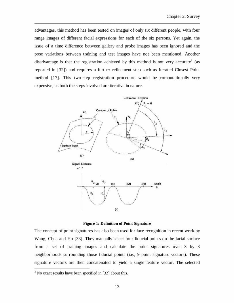
The concept of point signatures was proposed by Chua and Jarvis for the purpose of
object recognition from range data [31]. Consider the point p on the surface of an object
with a sphere of radius r placed around it (see Figure 1). The intersection of this sphere

Chapter 2: Survey ________________________________________________________________________
12
with the surface of the object is a curve C whose orientation can be defined by a normal
vector 1n , a reference vector 2n and their cross product. The vector 1n is the unit vector
normal to a plane P fitted through the curve C . A new plane 1P is defined by translating
the plane P to the point p in the direction of the normal vector 1n . The perpendicular
projection of the curve C onto the plane 1P forms the curve 1C with the projection
distance of the points on 1C forming a signed distance profile. The reference direction
2n is defined as the unit vector from p to the projected point on 1C which gives the
largest positive distance. Every point on the curve C is characterized by the signed
distance from itself to its corresponding point on the curve 1C and the clockwise rotation
from the direction 1n around the direction 2n . In typical implementations, the points on
the curve C are chosen at equal angular intervals θ∆ from 0 to 360 degrees. Thus, the
signature of each point can be represented as a vector of values )( id θ for i ranging from
0 to 360 degrees in steps of θ∆ .
A major advantage of the concept of point signature is its translation and rotation
invariance, without relying on any surface derivatives. Matching between two object
surfaces is performed by calculating the point signatures at each point on the two surfaces
and then correlating the point signature vectors to establish correspondence between the
points on both surfaces. From this, the relative motion between the two surfaces can be
estimated and finally the surfaces can be registered to evaluate an appropriate similarity
measure.
The concept of point signatures was extended to expression-invariant 3D face recognition
by Chua, Han and Ho [32]. For this purpose, the facial surface is treated as a non-rigid
surface. A heuristic function is first used to identify and eliminate the non-rigid regions
on the two facial surfaces (further details in [32]). Correspondence is established between
the rigid regions of the two facial surfaces by means of correlation between the respective
point signature vectors and other criteria such as distance, and finally the optimal
transformation between the surfaces is estimated in an iterative manner. Despite its
Chapter 2: Survey ________________________________________________________________________
13
advantages, this method has been tested on images of only six different people, with four
range images of different facial expressions for each of the six persons. Yet again, the
issue of a time difference between gallery and probe images has been ignored and the
pose variations between training and test images have not been mentioned. Another
disadvantage is that the registration achieved by this method is not very accurate2 (as
reported in [32]) and requires a further refinement step such as Iterated Closest Point
method [17]. This two-step registration procedure would be computationally very
expensive, as both the steps involved are iterative in nature.
Figure 1: Definition of Point Signature
The concept of point signatures has also been used for face recognition in recent work by
Wang, Chua and Ho [33]. They manually select four fiducial points on the facial surface
from a set of training images and calculate the point signatures over 3 by 3
neighborhoods surrounding those fiducial points (i.e., 9 point signature vectors). These
signature vectors are then concatenated to yield a single feature vector. The selected 2 No exact results have been specified in [32] about this.

Chapter 2: Survey ________________________________________________________________________
14
fiducial points include the nasal tip, the nasal base and the two outer eye corners. A
separate eigenspace is built from the point signatures in the 3 by 3 neighborhood
surrounding each fiducial point in each range-image. Thus, four different eigenspaces are
constructed in total. Given a test range image, the four fiducial points are first located.
For this, point signatures are calculated at the 3 by 3 neighborhood surrounding every
facial point, and represented as a single vector. The distance from feature space (DFFS)
[18] value is calculated between the vector at each point and the four eigenspaces. The
fiducial points correspond to those points at which the DFFS value with respect to the
appropriate eigenspace is minimal. For face matching, classification is performed using
support vector machines [11], with the input consisting of the point signature vectors at
the 3 by 3 neighborhoods surrounding the four fiducial points. The maximum recognition
rate with three training images and three test images per person is reported to be around
85%. The different images collected for each person show some variation in terms of
facial expressions. The authors do not mention the time gaps between the acquisition of
gallery and probe images, and they do not specify the effect of important parameters such
as the radius of the sphere required for calculating the point signatures. Furthermore, their
research takes into account information at only four fiducial points on the surface of the
face, which would seem to be inadequate from the point of view of robust facial
discrimination. They have also not given any statistical analysis of the errors in
localization of the facial feature points and its effect on recognition accuracy. It should be
noted that in a separate set of experiments, the authors have also made use of the
corresponding texture information besides the 3D shape, leading to a combined
recognition rate of around 91%.
(2.5) Using Kimmel’s Eigenforms
A novel non-rigid object recognition technique has been proposed by Kimmel et al in
[34]. It has been applied to the problem of expression-invariant face recognition in [35].
In this method, the facial surface is represented by a matrix of pair wise geodesic
distances between surface points. If the facial surface consists of N points, this leads to

Chapter 2: Survey ________________________________________________________________________
15
an N x N matrix of geodesic distances, that is each individual point is effectively
represented as an N -tuple. This matrix is then projected onto a three-dimensional space
using a distance-preserving dimensionality reduction technique such as Multidimensional
Scaling [37]. Geodesic distances are essentially invariant to translation, rotation and any
surface deformation that does not involve tearing. As a result, the lower-dimensional
embedding is also invariant to all these transformations, and therefore provably invariant
to changes in facial expression. This three-dimensional embedding has therefore been
called the “bending invariant canonical form”. These bending invariant canonical forms
are then aligned (further details in [36]) and interpolated onto a Cartesian grid giving a
“canonical image”. An eigenspace is created from the canonical images of the gallery
images of each person. The probe images are subjected to the same transformations and
are used for matching. Despite the inherent advantages of this technique and its
robustness to facial expressions, no recognition results whatsoever have been reported in
either [34] or [35].
(2.6) Methods Based on Iterated Closest Point
The Iterated Closest Point (ICP) algorithm was proposed by Besl and McKay [17] for the
purpose of registering rigid 3D point clouds (free-form surfaces). Given two 3D surfaces
to be registered, this method treats one of the surfaces as the model surface and the other
as the probe. It aims to iteratively move the probe so that it is aligned as close to the
model as possible. The method employs the nearest Euclidian neighbor heuristic to
establish a rough correspondence between points on the two surfaces. In other words, for
each point on the probe surface, it computes the closest point on the model surface and
treats that as the corresponding point. The pairs of roughly corresponding points are
given as input to a least-squares technique to estimate the relative motion. This motion is
then applied to the probe surface and the mean squared error between the corresponding
points on the probe and the model is computed. These four steps are repeated until the
change in the mean squared error between successive iterations drops below a certain
threshold. Besl and McKay explicitly prove that the mean squared error between the

Chapter 2: Survey ________________________________________________________________________
16
corresponding points in the two surfaces undergoes a monotonic decrease until it reaches
a local minimum [17]. However, the ICP algorithm assumes that the two surfaces are
initially in approximate alignment, and it can fail under noise or occlusion [17]. Chen and
Medioni [38] have proposed a modification to this method, which involves point to plane
distances instead of point-to-point distances. Their method is known to be less
susceptible to local minima, but it suffers from the problem of much slower speed [38].
Lu, Colbry and Jain have also used an ICP-based method for facial surface registration in
[39] and [40]. They have employed a feature-based algorithm followed by a hybrid ICP
algorithm that alternates in successive iterations between the method proposed by Besl &
McKay [17] and the method proposed by Chen and Medioni [38]. In this way they are
able to make use of the advantages of both algorithms: the greater speed of the algorithm
by Besl and McKay [17], and the greater accuracy of the method by Chen and Medioni
[38]. Their hybrid ICP algorithm has been tested on a database of 18 different individuals
with frontal gallery images and probe images involving pose and expression variations. A
probe image is registered with each of the 18 gallery images and the gallery giving the
lowest residual error is the one that is considered to be the best match. Using the residual
error alone, they obtain a recognition rate of 79.3%. They improve this recognition rate to
84% by further incorporating information such as shape index and texture.
(2.7) Morphable Models
Although the focus of this thesis is face recognition from only 3D shape information, for
the sake of completeness, we present a very brief overview of the technique of morphable
models, proposed by Romdhani, Vetter and Blanz, which makes use of a statistical 3D
model to perform recognition from 2D images [41], [42]. Basically, they use an
appearance-based method for face recognition and construct a morphable model for the
synthesis of 3D faces. A morphable face model is constructed by transforming the shape
and texture (regarded as albedo values) of a set of exemplars of 3D face models into a
vector space representation. This transformation to an orthogonal co-ordinate system,
formed by eigenvectors is performed using Principal Components Analysis [18]. The

Chapter 2: Survey ________________________________________________________________________
17
novel shape and texture of any face can now be expressed as a linear combination of the
shape and texture eigenvectors. The shape and texture coefficients of the morphable
model constitute a pose, scale and illumination-invariant low dimensional encoding of the
identity of a face. This is because the shape and texture eigenvectors are derived from
characteristics pertaining only to identity (3D shape and albedo). It is these coefficients
that are used to recognize faces. The morphable face model is generative, which means
that it can produce photo-realistic face images. The model undergoes a rendering process
that transforms the given face shape and texture vectors into an image. The 3D shape is
subjected to rigid transformations and perspective projection to yield the 2D image co-
ordinates. Expressing an input image in terms of model parameters is performed using an
analysis-by-synthesis loop in which an image is generated in each iteration using the
current estimate of the model parameters. Then, the difference between the model image
and the input image is computed, and an update of the model parameters that reduces this
difference is performed. This is a minimization problem whose cost function is the image
difference between the image rendered by the model and the input image. The shape and
pose parameters are updated using the shape error estimated by the optical flow between
the rendered image and the input image. Finally, the obtained shape and texture
coefficients corresponding to the input image are matched with those of a known
individual. The matching criterion used is a simple nearest neighbor classification rule
using a correlation-based similarity measure. The results reported in [42] using this
technique are from the CMU-PIE database [43] consisting of images of 68 individuals
with lighting, pose and expression variations. Using a single frontal gallery image per
individual, a recognition rate of 97% has been reported for frontal probe images. The
recognition rate drops down to 91% and 60% respectively when semi-profile and profile
images are used.

Chapter 2: Survey ________________________________________________________________________
18
Reference 2D
or
3D
or
both
Number of
individuals
Number
of
training
images
per
individual
Number
of test
images
Manual or
automatic
pose
normalization
Time gap
between
training
and test
image
acquisition
Recognition
rate with
one training
image at
rank one
[19]
(2002)
3D 37 1 185 Automated Not given 83%
[19]
(2003)
3D 295 1 295 Not done No time
gap, test
images
generated
by rotating
training
images
93% for 2-3
degree
rotation, to
85% for 10
degree
rotation
[19]
(2003)
Both 295 1 295 Not done No time
gap, test
images
generated
by rotating
training
images
97.5%
[20]
(1997)
3D 24 5 120 Automated Not
specified
100%
[22]
(2003)
3D 200 1 870 Manual 6 to 13
weeks
92.8%
[22]
(2003)
2D
and
3D
200 1 870 Manual 6 to 13
weeks
98%
[23]
(1998)
3D 37 1 37 Automated Not
specified
100%
[25] 3D 6 1 6 Automated Not Not reported
Chapter 2: Survey ________________________________________________________________________
19
(1990) specified
[26]
(1991)
3D 26 26 24 Automated Not
specified
100%
[27]
(2003)
3D 60 1 360 Automated Not
specified
78%
[29]
(2003)
3D 35 1 70 Automated Not
specified
94% at rank
5
[31]
(2000)
3D 6 4 6 Automated Not
specified
100%
[32]
(2002)
3D 50 1 250 Automated Not
specified
85%
[32]
(2002)
Both 50 1 250 Automated Not
specified
91%
[34]
(2003)
3D 157 Not
specified
Not
specified
Automated Not
specified
Not
specified
[38]
(2004)
3D 18 1 63 Automated Not
specified
79.37%
[38]
(2004)
Both 18 1 63 Automated Not
specified
84.13%
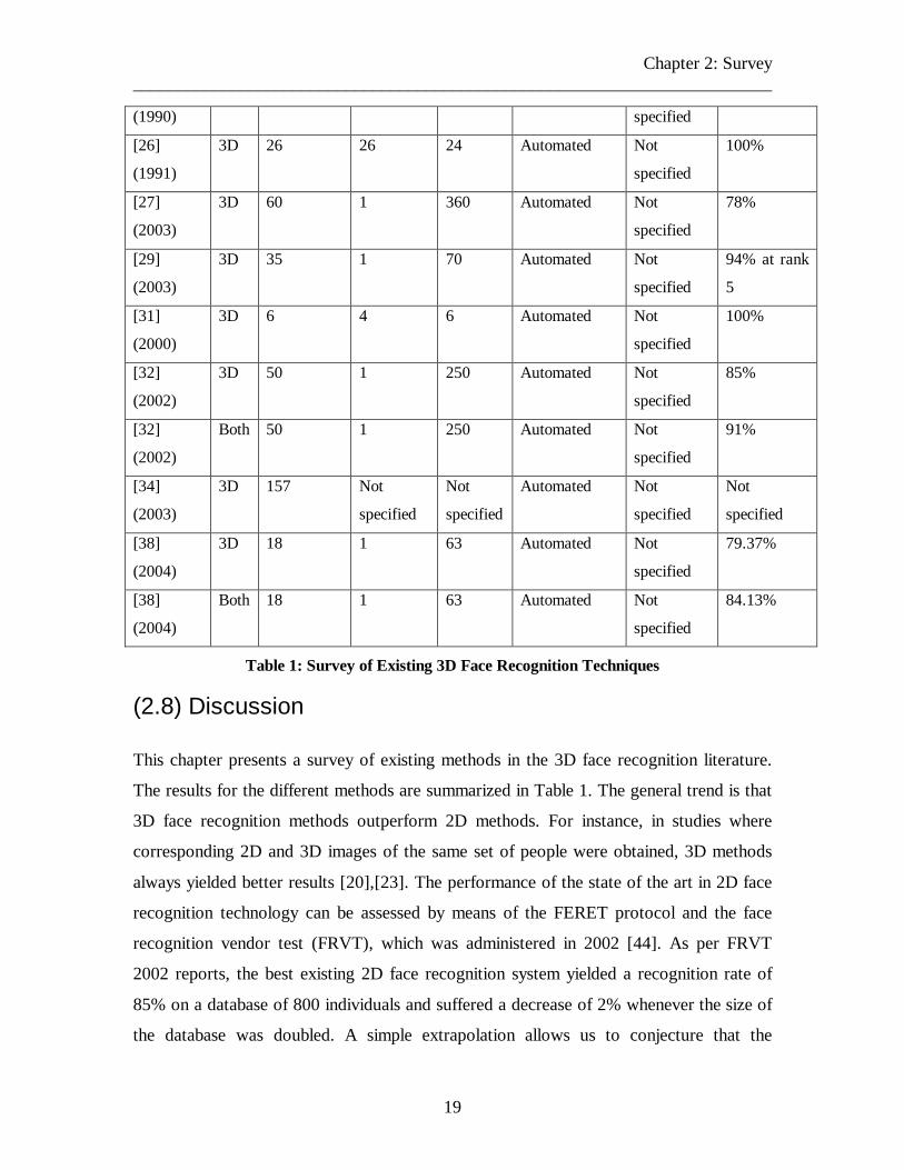
Table 1: Survey of Existing 3D Face Recognition Techniques
(2.8) Discussion
This chapter presents a survey of existing methods in the 3D face recognition literature.
The results for the different methods are summarized in Table 1. The general trend is that
3D face recognition methods outperform 2D methods. For instance, in studies where
corresponding 2D and 3D images of the same set of people were obtained, 3D methods
always yielded better results [20],[23]. The performance of the state of the art in 2D face
recognition technology can be assessed by means of the FERET protocol and the face
recognition vendor test (FRVT), which was administered in 2002 [44]. As per FRVT
2002 reports, the best existing 2D face recognition system yielded a recognition rate of
85% on a database of 800 individuals and suffered a decrease of 2% whenever the size of
the database was doubled. A simple extrapolation allows us to conjecture that the

Chapter 2: Survey ________________________________________________________________________
20
performance of this system on a database of 200 individuals would be around 89%. On
the other hand, the largest 3D face recognition system (developed by Chang [23]) yields a
performance of about 92.8% on a database of 200 individuals, thereby outdoing the best
existing 2D face recognition method. A combination of 2D and 3D methods has been
reported to yield much higher rates than either 2D or 3D alone [23],[20], [33] (also see
Table 1). However, it should be noted that the focus of this thesis is to make use of only
3D shape information, ignoring texture completely.
(2.9) Overview of the Recognition Method Followed
Before a facial scan under test can be matched to a database of individuals, the scan must
be normalized for pose variations. In this thesis, a fully automated facial normalization
step is employed in order to align a range-image under test to as closely frontal a pose as
possible. The normalization step consists of two stages. In the first stage, salient feature
points are detected and a coarse normalization of the probe-images is performed. In the
second stage, the normalization is further refined using an extension of the ICP algorithm
[17] that has been proposed in this thesis. The original ICP algorithm uses only the
coordinates of the points on the surface in order to establish point-to-point
correspondence. The proposed extension additionally incorporates local surface
properties such as local moment invariants and surface curvature in order to improve the
correspondence step of the ICP algorithm. It also employs simple heuristics to discard
outliers in the data. This version of ICP is shown to outperform the original algorithm and
is used as a subsequent step, after feature-based normalization. The integrated two-stage
algorithm yields very low point-to-point residual error values when the images being
matched belong to one and the same person, and higher values if the images belong to
different individuals. Hence the error values can be treated as reliable similarity metrics
to ascertain identity.
It should be noted that the feature-based method requires the detection of both the eyes
on the facial surface and therefore will fail for extreme profile views of the face (typically
beyond +/- 50 degrees of yaw). To perform recognition from facial scans in such views,

Chapter 2: Survey ________________________________________________________________________
21
the feature-based step can be replaced by the learning method for pose-estimation
described in chapter (3). This approach, which uses support vector regression [11], can
robustly predict the approximate pose within an error of +/- 9 degrees. Using the
predicted pose values, the facial scan can be rotated to a near frontal pose.
The basic strategy employed here is most similar to the method adopted by Lu and Jain in
their very recent work [39]. However, their method does not incorporate local surface
properties during the ICP iterations. Instead, they make use of curvature (and texture)
information in addition to the final residual error as a combined similarity metric. Our
algorithm has been tested on a database containing many more individuals and yields
much superior results (a recognition rate of 91.5%). Furthermore, as will be detailed in
chapter (4), we have also measured the recognition rates for different poses of the probe
images. The methods for face recognition adopted in this thesis, along with the
corresponding results, are described in more detail in Chapter (4).
To summarize, our method has the following advantages over existing 3D face
recognition methods:
• It has given a high recognition rate of 91.5% on a large database of 200
individuals. The recognition rate is slightly less than that reported in [23] but their
method requires manual intervention, unlike ours, which is fully automated.
• It has been tested on a database [23] in which there was a significant time gap
(ranging from 6 to 13 weeks) between the acquisition of the gallery and probe
images. Most existing 3D face recognition methods have not ensured this (see
Table 1).
• It is robust to a wide range of poses including extreme profile views by
incorporation of the learning-based pose prediction algorithm discussed in
Chapter (3).
Chapter 3: Facial Pose Estimation ________________________________________________________________________
22
Chapter Three: Facial Pose Estimation
This chapter firstly discusses the basic need for pose estimation techniques in a face
recognition system. It also reviews existing techniques for facial pose estimation from 2D
and 3D data. Thereafter, the approach adopted in the thesis for determining facial pose is
explained in detail. It is observed that there is an inherent similarity between the facial
shapes of different people in similar poses. A machine learning technique is followed to
make use of this similarity in order to arrive at a generic relationship between 3D facial
shape and 3D facial pose. Experimental results on the accuracy of the method are
reported in detail on a large test set. This is followed by an examination of the effect of
range image size on the accuracy of the pose estimation results. Some experimental
results are reported on the effect that dimensionality reduction of facial range images
(using PCA) has on the accuracy of pose estimation.
(3.1) Need for Facial Pose Estimation Techniques Although 3D face recognition methods are more or less invariant to changes in
illumination, variation in facial pose still remains a major issue. It has been observed that
face recognition techniques are very sensitive to even minor head rotations. This gives
rise to the need for a robust and automated system to obtain accurate head pose. Facial
pose estimation can also be a vital step in effective view-invariant face detection from 2D
or 3D scenes or face tracking and surveillance applications. The estimation of pose is
generally a more difficult problem in 2D owing to changes in illumination. In 3D, the
problem is ostensibly simpler as 3D data are independent of illumination. However the
distribution of 3D facial shapes across the view-sphere is still quite complex. Differences
in individual identity, facial expression and occlusions further contribute to this
complexity. All these factors give rise to the basic need for developing a module that can
perform estimation of facial pose to a good degree of approximation, in a manner that is
independent of identity.

Chapter 3: Facial Pose Estimation ________________________________________________________________________
23
(3.2) Review of Existing Literature
The problem of identity invariant facial pose estimation has not received much attention
in the computer vision literature. The existing pose estimation methods can be broadly
classified into feature-based and appearance-based methods. Feature-based methods
try to estimate pose based on geometric relationships between certain salient facial
features, whereas the latter category treats the face as a global entity. The following
subsections present a detailed review of the methods adopted for facial pose estimation
from 2D as well as 3D data. Many of the techniques for facial pose estimation from 2D
data are, however, also readily extensible to 3D data.
(3.2.1) Feature-Based Methods
The feature-based methods try to automatically locate salient facial features such as the
eyes, the nose and the mouth in the facial range or intensity image. The facial pose is then
calculated based upon the spatial arrangement of these features in comparison to that of a
reference face. Examples of existing feature-based methods include [45], [46]. In [45],
Krüger et al have used the method of elastic bunch graphs to locate faces in images and
ascertain their pose. They represent the face as a connected graph whose nodes consist of
Gabor jets. Different graph models are required for facial images in different poses. The
main drawback of this method is that it is computationally very demanding. In [46],
Hattori et al estimate the position of the eyes and eyebrow ridges from range and
intensity images. From this information, they estimate the facial vertical symmetry plane
and calculate the pose of the face from the equation of this plane. However, the basic
drawback of this and other feature-based methods is that the feature-detectors are
inherently sensitive to noise in data or minor aberrations. Furthermore, the apparent shape
of the individual facial features itself undergoes changes across the view-sphere. For
instance, the apparent shape of the eyes or the mouth is significantly different in profile
views or views with a large tilt as compared to exactly frontal poses. Owing to this fact,
these methods will be prone to produce several false matches if the range of poses is very
large. Hence feature-based methods should be used only in cases where the approximate
pose of the face is known, or where the range of poses to be dealt with is restricted.

Chapter 3: Facial Pose Estimation ________________________________________________________________________
24
(3.2.2) Appearance Based Methods
In contrast to feature-based methods, the appearance-based methods consider the facial
image as a global entity. Many of these methods make use of some learning algorithm to
develop a relationship between faces and poses. The basic assumption underlying most of
these methods is that faces of different individuals in similar poses show a marked
similarity [16]. In fact, images of different individuals in similar poses are in closer
resemblance with each other as compared to those of the same individual in different
poses [16]. This assumption holds true generally only for significant changes in pose.
The earliest work on this problem (from 2D images) was by Pentland and Moghaddam,
and was based on Principal Components Analysis (PCA) [47]. They introduce the
concept of view-based Eigenspaces. They take an ensemble of images of people in
different poses from –90 to +90 degrees around the Y-axis with an angular sampling of
10 degrees and construct a view-based eigenspace for images in each pose. The pose of a
test-face is estimated by calculating its distance to each view-based Eigenspace, and
selecting the pose-class with the least distance. The performance of a view-based face
detector using this technique can be further improved by using calculating the likelihood
value that a test-face belongs to a certain pose-class. The pose-class with the maximum
likelihood value is selected. This method has been proposed by Moghaddam and
Pentland in [48].
Nayar and Murase [49] perform object pose estimation and recognition simultaneously
by creating a universal Eigenspace. The universal Eigenspace is created from an
ensemble of images of various objects, each in different poses. This method is trivially
extensible to poses of human faces. Srinivasan and Boyer [50] have replaced the distance
from feature space metric used in [47] by an energy function, which is basically equal to
the norm of the vector of eigen-coefficients of a test-image projected onto a particular
view-based Eigenspace. This energy function is directly proportional to the similarity
between the test-image and the templates of that pose-class and can be used for the
purpose of pose-estimation.

Chapter 3: Facial Pose Estimation ________________________________________________________________________
25
In [51], Wei et al also propose a pose estimation method that is based on Principal
Components Analysis [18]. They first use orientation-specific Gabor filters to normalize
the facial images for changes in illumination and then create view-based eigen-spaces out
of these filtered images. They use both distance from feature space (DFFS) and distance
in feature space (DIFS) as a combined metric to determine pose [51]. Their paper claims
a superior performance to ordinary view-based Eigenspaces owing to the pre-processing
step wherein they achieve illumination invariance. In [52], the PCA step to determine
facial pose is preceded by a stage involving the computation of a three-level discrete
wavelet transform (instead of Gabor filters). The Eigenspaces are computed out of only
the LL sub-bands of the facial images to make the algorithm more robust to noise and
illumination.
It has been claimed that the distribution of faces with changes in illumination and
expression is too complex to be modeled adequately by linear techniques such as PCA
[53]. In [53], a kernel-based machine learning approach called Kernel Principal
Components Analysis (KPCA) is followed to obtain a non-linear mapping between faces
and poses. Facial images are collected in different poses from 0 to 90 degrees around the
Y-axis in steps of 10 degrees. For each view, KPCA is performed by mapping the images
in the input space to a higher-dimensional space using a kernel function. This is followed
by PCA on the higher-dimensional space to ultimately obtain lower-dimensional eigen-
coefficients per training sample. A support vector classifier [11] is then trained to
recognize the feature-vectors of each single view using vectors of that view as positive
examples, and vectors of other views as negative examples. Thus given a test image, its
projection onto each KPCA space is calculated to obtain the respective feature-vectors.
The pose of the test image is predicted from the cumulative output of all the view-based
support vector classifiers. The results obtained with this method are 97.52% within a +/-
10-degree accuracy. However, the main disadvantage of this method is the computation
of a pair wise kernel distance matrix, whose size increases quadratically with the number
of training images per view. Secondly, it also requires the training images to be present in
memory at the time of actual pose estimation.
Chapter 3: Facial Pose Estimation ________________________________________________________________________
26
Nandy and Ben-Arie create a 3D volumetric frequency-domain representation of an
object denoted as VFR [54]. The VFR of an object represents both its spatial structure as
well the “continuum” of the 2D discrete Fourier Transform of its views. Pose estimation
is carried out by using a VFR model constructed from a person’s 3D scan. Gray-level
images of the person are used to index into this VFR model employing the Fourier Slice
Theorem.
Krüger et al have combined Gabor Wavelets with RBF networks to create Gabor Wavelet
networks for the purpose of pose estimation [55]. This method suffers from poor
generality, as neural networks do not generalize well to previously unseen facial images.
Furthermore, neural networks suffer from several convergence-related issues at the time
of training. Computation of Gabor Wavelets is also quite expensive.
Support Vector Machines (SVMs) have been used in the past for the purpose of pose
estimation. Huang et al [56] used SVMs to classify three different poses around the Y-
axis, separated by 30 degrees. Support vector classification (SVC) can be
computationally cumbersome, especially if the number of pose-classes is high, as it
requires a “one-against-rest” or “one-against-one” classification method to be employed.
Support vector regression (SVR) is an interesting alternative that has been used for facial
pose estimation from 2D Sobel edge-images, by Gong et al [57]. They have applied it to a
training set consisting of yaw changes from -90 to +90 and tilt changes from –30 to +30
degrees, and claim an average pose estimation error of 10 degrees for either angle.
Very little research has been done so far on estimation of the pose from any arbitrary 3D
scan of a human head, though many of the above-mentioned techniques are easily
extensible to 3D data as well. Existing methods for 3D data include one by Sarris et al
[59], wherein an ellipsoid is fit to a set of 3D points lying on a human face. The pose is
estimated from the major and minor axes of this ellipsoid. Another method includes a
head-tracking system developed by Malassiotis and Strintzis [58]. Their method consists
of projecting the 3D human head onto a previously created pose eigen-space. The pose of

Chapter 3: Facial Pose Estimation ________________________________________________________________________
27
the rotating head is estimated continuously by calculating the likelihood that the head
belongs to a certain pose, and also making use of a state transition model, thereby taking
into account the pose of the rotating head at the previous instant. However this method
does not solve the problem of estimating the pose of a single 3D scan based on the typical
shape of a face in a certain pose.
(3.3) Approach Followed
In this thesis, we assume that there is an inherent similarity between the 3D shape of
faces of different individuals in similar poses and use a learning method to exploit this.
We use a combination of the Discrete Wavelet Transform [60] and either Support Vector
Regression [11] or Discriminant Isometric Mapping [15], to arrive at a generic
relationship between faces and poses, the latter being defined in terms of the angles of
rotation around the Y- and X-axes. The method described in this thesis is the first attempt
to develop such a generic relationship between pose and 3D facial shapes in different
poses. It is specifically designed to predict the pose from a single 3D scan of a person,
making use of only the model developed by the machine-learning algorithm.
(3.4) Using Support Vector Regression
This section describes the pose estimation module using support vector regression.
Firstly, the theory of support vector regression is briefly reviewed followed by a
description of the experimental set-up. The use of the discrete wavelet transform as a pre-
processing step is discussed. The data set on which the learning algorithm was trained
and tested is described and the results of the pose estimation accuracy are presented. This
is followed by a series of experiments that show how the accuracy of the results varies
with different factors: namely, with the change in angular sampling between successive
poses during training, with the change in input image size and also with reduction in the
dimensionality of the input patterns.
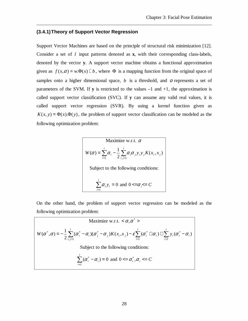
Chapter 3: Facial Pose Estimation ________________________________________________________________________
28
(3.4.1) Theory of Support Vector Regression
Support Vector Machines are based on the principle of structural risk minimization [12].
Consider a set of l input patterns denoted as x, with their corresponding class-labels,
denoted by the vector y. A support vector machine obtains a functional approximation
given as bxwxf +Φ= )(.),( α , where Φ is a mapping function from the original space of
samples onto a higher dimensional space, b is a threshold, and α represents a set of
parameters of the SVM. If y is restricted to the values –1 and +1, the approximation is
called support vector classification (SVC). If y can assume any valid real values, it is
called support vector regression (SVR). By using a kernel function given as
)().(),( yxyxK ΦΦ= , the problem of support vector classification can be modeled as the
following optimization problem:
Maximize w.r.t. α
),(2
1)(
1,1jijij
l
jii
l
ii xxKyyW αααα ��
==
−=
Subject to the following conditions:
01
=�
=i
l
ii yα and Ci<=<=α0
On the other hand, the problem of support vector regression can be modeled as the
following optimization problem:
Maximize w.r.t. >< *,αα
���===
−++−−−−=l
iiii
l
iiijijj
l
jiii yxxKW
1
*
1
**
1,
** )()(),()()(2
1),( ααααεαααααα
Subject to the following conditions:
0)(1
* =−�
=i
l
ii αα and Cii <=<= αα ,0 *

Chapter 3: Facial Pose Estimation ________________________________________________________________________
29
Here the factor C denotes a tradeoff between the simplicity of the function f and the
amount to which deviations larger than ε (the regression error) will be tolerated. The
basic aim of support vector regression is to find a function )(xf , which has a deviation
of not more than ε from the provided output values for all the training samples and
which at the same time is as “flat” as possible. This corresponds to having a minimal
norm of the vector w in the expression bxwxf +Φ= )(.),( α .
The solution to this problem is given by the following equation:
bxxKxfl
iiii +−= �
=),()()(
1
* αα
In most cases, only a small fraction of the training samples have non-zero values of α . It
is solely these examples that influence the final decision function, and these are referred
to as the “support vectors” . In any regression or classification function, a smaller number
of support vectors is desirable to obtain as simple a function as possible. A large number
of support vectors is an indication of overfitting.
The significance of using kernel functions is that they perform an implicit (and efficient)
mapping onto a higher dimensional space and improve the separability between the
different classes of the training data [11], [13]. It is the kernel functions that allow the
support vector machine to fit non-linear functions on the training data. For a set of
training points denoted as u , the computation of a mapping )(uφ onto a higher
dimensional feature space, followed by SVR in that space, would be computationally
very expensive [11],[13]. Kernels are an elegant workaround as they allow computation
of the inner product ),()().( 2121 uuKuu =φφ without ever explicitly computing the
mapping φ . This property holds true for all kernels that satisfy Mercer’s condition [13].
The reader is referred to [11], [12], [13] for the finer mathematical treatment and proofs
of all the aforementioned results.

Chapter 3: Facial Pose Estimation ________________________________________________________________________
30
(3.4.2) Motivation for using Support Vector Regression In this thesis, support vector machines have been employed to create a generic model to
learn the relationship between faces and their respective poses. The basic reason for
preferring them over other popular learning techniques such as neural networks are
outlined below:
• Support vector machines allow the fitting of highly non-linear functions to the
training data without getting stuck in local minima [14].
• They require tweaking of a very small number of parameters [14].
• Results of the SVM optimizations are not dependent upon issues such as the
starting point as in the case of neural networks. The final results are independent
of the specific algorithm being used for the optimization [14].
• The basic functioning of the SVM is independent of the choice of the kernel
function [14].
• In most cases, as described in the above section, only a small percentage of
training examples actual influence the function estimation. This fact makes SVMs
a computationally much more efficient alternative in comparison to other learning
techniques such as KPCA which do not discard the “unimportant” training
examples [53]. Moreover, the latter method requires the calculation of a pair wise
distance matrix between all the training points.
• Support vector machines using kernel functions are preferable to linear methods
such as PCA for the purpose of pose estimation. This is because the complexity of
pose distribution of human faces under varying identity, expression or occlusion
cannot be adequately modeled by linear methods [53].
It should be noted that as the pose of a face is a continuous real-valued entity, regression
is preferable to classification for the specific purpose of pose-estimation.

Chapter 3: Facial Pose Estimation ________________________________________________________________________
31
(3.4.3) Experimental Setup
To be able to predict the pose of any given face, the support vector machine first needs to
be trained on a set of labeled examples. These examples consist of several poses of a
chosen number of faces. The poses in the training set must cover the entire range of
poses, which the support vector machine has to “ learn” . The facial images in different
poses are labeled by the appropriate angles. Using a suitably chosen kernel, the support
vector machine then uses these examples to learn a model. The model learnt by the SVM
is tested on a large number of poses of a set of “test faces” . All the test faces belong to
individuals strictly different from those included in the training set. The poses considered
consist of combined rotations around the Y-axis (called “yaw”) and rotations around the
X-axis (called “tilt” ). Basically, two different support vector machines are employed, one
to predict the yaw and the other to predict the value of the tilt.
The structure of the training and test sets employed in this thesis is described in detail in
sections (3.4.5) and (3.4.7).
(3.4.4) Use of Discrete Wavelet Transform
A discrete wavelet transform (using Daubechies-1 wavelets, also called Haar wavelets) is
performed on all the range-images before giving them as input to the SVM, both at the
time of training as well as testing. The discrete wavelet transform decomposes an image
into four different sub-bands: the LL sub-band, which consists of low frequency
components in both row and column directions, the HH sub-band which consists only of
high frequency components in both directions, and the HL and LH sub-bands which
consists of low-frequency components in exactly one of the two directions. Of all the four
sub-bands, the LL sub-band is the one that is most noise-free. In all the experiments, only
the LL sub-bands have been given as an input to the SVM.
One major advantage of using the Discrete Wavelet Transform is that it improves
computational efficiency greatly. A single-level DWT gives rise to an LL sub-band that is
one-fourth the size of the original image. In all the experiments, the level of wavelet

Chapter 3: Facial Pose Estimation ________________________________________________________________________
32
decomposition was chosen to be three, giving rise to an LL sub-band that is 64 times
smaller in size than the original image. The second advantage of using the DWT is that
the low frequency information in the LL sub-bands is known to accentuate pose-specific
details, suppress individual facial details, and be relatively invariant to facial expressions
[52]. Convolving the images with Gabor wavelets is also another method of accentuating
pose-specific information, as reported in [51]. However this method is computationally
expensive and also requires careful selection of various Gabor wavelet parameters such
as center frequency, scale and kernel-size.
(3.4.5) Sources of Data
The data for the experiments in this thesis was collected from two sources, the first being
the set of eigenvectors of manually aligned 3D shapes of human faces, provided by the
University of Freiburg [41]. As per the morphing method explained in [41], 100 new
faces were obtained. The morphing method consists primarily of taking a linear
combination of the provided eigenvectors to generate new shapes. The geometry of a face
can be represented as a shape vector ),,( iii ZYXS = where 1=i to N . The mean shape
as well as the shape eigenvectors can all be expressed in this format. A new and realistic
looking facial shape can be generated using the formula ii
M
iimeannew SSS σα
�
=+=
1
where
meanS is the mean shape (shown in Figure 2), M is the total number of shape eigenvectors
(49 in this case), iS are the eigenvectors, iσ are the eigenvalues, and iα are coefficients
that are randomly picked between +3 and –3. In this way, several new and realistic-
looking facial shapes can be easily created. All the faces thus morphed were in exact
frontal pose (0 degree head rotation about either axis).
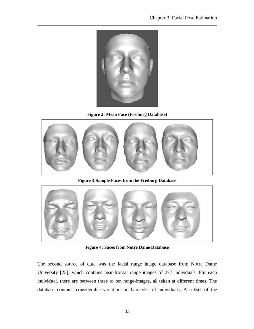
Chapter 3: Facial Pose Estimation ________________________________________________________________________
33
Figure 2: Mean Face (Freiburg Database)
Figure 3:Sample Faces from the Freiburg Database
Figure 4: Faces from Notre Dame Database
The second source of data was the facial range image database from Notre Dame
University [23], which contains near-frontal range images of 277 individuals. For each
individual, there are between three to ten range-images, all taken at different times. The
database contains considerable variations in hairstyles of individuals. A subset of the

Chapter 3: Facial Pose Estimation ________________________________________________________________________
34
range-images in this database also contains slightly different expressions for one and the
same individual.
(3.4.6) Pre-Processing of Data for Pose Estimation Experiments
Since the faces of the Freiburg database were in the form of point-clouds, a surface
reconstruction step was necessary. This was performed using the “Power Crust Surface
Reconstruction Algorithm” [66]. To obtain training data in all possible poses for the
pose-estimation experiments, the facial surfaces were suitably projected onto different
view-planes across the view-sphere using the well-known Z buffer algorithm [67]. This is
actually equivalent to rotating the facial surface, but is much more efficient to implement.
The view-sphere was suitably sampled so as to obtain all views of the face corresponding
to combined rotations from 0 to +90 degrees around the Y- and from -30 to +30 degrees
around the X-axis in steps of δ degrees.
For the purpose of generating a good data set for pose-estimation, an initial step that
involved manual alignment of the range images of the Notre Dame database was
required, in order to try to create nearly exact frontal poses. For this the positions of the
eyes were marked manually, the line joining the eyes was aligned with the horizontal and
the nasal ridge was aligned with a fixed line, at 30 degrees w.r.t. the Y-axis. Range
images that contained holes (missing data) were passed through a simple averaging filter.
Portions of the images exterior to the facial contour were manually cropped. Different
poses of each face were generated by projection onto different view-planes, as described
above.
Finally, all range images were resized to 160 by 160, taking care to preserve the aspect
ratio and padding an appropriate number of zeroes. A few faces from the Freiburg and
Notre Dame databases, after the application of filtering and pre-processing techniques,
are shown in Figure 3 and Figure 4.
Chapter 3: Facial Pose Estimation ________________________________________________________________________
35
(3.4.7) Training Using Support Vector Regression
For the purpose of training, two different SVMs were used in the pose estimation
experiments. One was for learning a relationship between range images and their Y-
angle, and the other for learning the relationship between range images and their X-angle.
The available data were divided into non-intersecting training and test sets. The training
data consisted of all poses from 0 to +90 degrees around the Y-axis and -30 to +30
degrees around the X-axis in steps of three degrees. Fifty individuals each from the
Freiburg and Notre Dame databases were selected. The rest of the faces were used for
testing. Two different SVM-based estimators were developed using the LIBSVM
package [68]. A radial basis function kernel given by ))(exp(),( 2yxyxK −−= γ with
parameters γ = 0.03125 was chosen for both estimators. The parameter C for the SVM
was selected to be 64, and the value of the regression-marginε was chosen to be 1.0.
These values were found by means of cross-validation on the training data using a simple
“grid-search” tool provided within the LIBSVM package [68]. The original range images
of size 160 by 160 were converted to sub-bands of size 20 x 20 after level-3 wavelet
decomposition. Each range image was thus represented as a 1 x 400 vector. These
vectors, labeled by their pose, were given as input to the SVMs. The number of support
vectors was observed to be approximately 12% and 14% of the number of training
samples when creating a functional approximation for the Y- and X-angle, respectively.
(3.4.8) Testing Using Support Vector Regression The functions yielded by the SVM were tested on all of the different poses of the test
faces. The test images were also decomposed using a level 3 discrete Haar wavelet
transform and the LL sub-band was given as input to the SVM for testing. The test set
always consisted of individuals different from those in the training set. To confirm the
stability of the approach, the individuals in the training and test sets were randomly
exchanged. The experiments were repeated over 30 times. The pose-estimates were
compared with the known ground-truth values of both the Y- and X-angles in every
single run.

Chapter 3: Facial Pose Estimation ________________________________________________________________________
36
Experimental Results with SVR
A detailed study was performed that tested the effect of variations in the following
parameters on the accuracy of the model created by the SVM:
1) Angular Sampling in both the directions
2) Range-image size
3) Dimensionality Reduction
Angular Sampling
Initial experiments were performed with the angular sampling size δ� to determine its
optimum value. Figure 5 illustrates the variation of regression accuracy with respect toδ .
Clearly, the mean error in pose estimation bears a direct linear relationship with the
angular sampling. A value of δ =3 degrees provides the best performance. Thus, in all the
experiments reported below, angular sampling is set to 3 degrees to obtain as accurate a
pose model as possible, albeit at the cost of greater training time and required storage.
Smaller values of δ did not improve the performance much further as seen in Figure 5
and the training time and storage were significantly higher. Table 2 summarizes the
average pose-estimation results obtained over all 30 runs3. It should be noted that the
results did not vary widely across the 30 different runs. This confirms the stability of the
model.
The histograms of estimation error versus head pose angle (yaw and tilt) are shown in
Figure 6 and Figure 7 respectively. For the Freiburg database, the mean error (i.e., mean
value of the absolute difference between the actual and predicted pose) is 2.8 degrees and
2.58 degrees for the Y- and X-angles, respectively. For the Notre Dame database, the
mean error is 3.2 degrees and 2.72 degrees for the Y- and X-angles respectively. The
mean error reported in [58] is less than 2 degrees. However, as noted in section (3.2.2),
3 For δ=3 degrees.
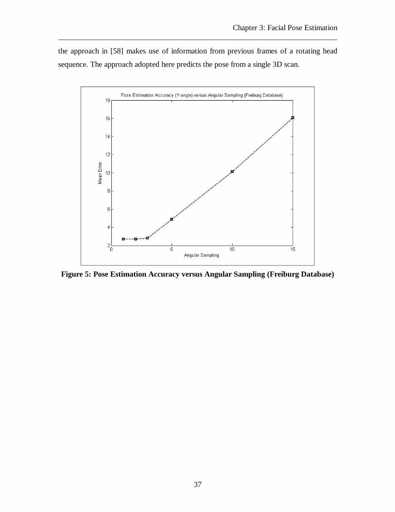
Chapter 3: Facial Pose Estimation ________________________________________________________________________
37
the approach in [58] makes use of information from previous frames of a rotating head
sequence. The approach adopted here predicts the pose from a single 3D scan.
Figure 5: Pose Estimation Accuracy versus Angular Sampling (Freiburg Database)
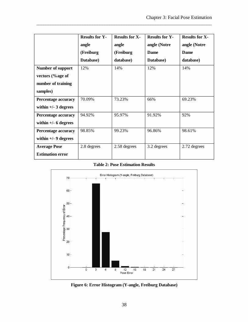
Chapter 3: Facial Pose Estimation ________________________________________________________________________
38
Results for Y-
angle
(Freiburg
Database)
Results for X-
angle
(Freiburg
database)
Results for Y-
angle (Notre
Dame
Database)
Results for X-
angle (Notre
Dame
database)
Number of support
vectors (%age of
number of training
samples)
12% 14% 12% 14%
Percentage accuracy
within +/- 3 degrees
70.09% 73.23% 66% 69.23%
Percentage accuracy
within +/- 6 degrees
94.92% 95.97% 91.92% 92%
Percentage accuracy
within +/- 9 degrees
98.85% 99.23% 96.86% 98.61%
Average Pose
Estimation error
2.8 degrees 2.58 degrees 3.2 degrees 2.72 degrees
Table 2: Pose Estimation Results
Figure 6: Error Histogram (Y-angle, Freiburg Database)

Chapter 3: Facial Pose Estimation ________________________________________________________________________
39
Figure 7: Error Histogram (X-angle, Freiburg Database)
Effect of range image size
In order to examine the effect of range image scale on facial pose estimation from range
data, the same experiments were performed on range images of different sizes: 320 x 320,
240 x 240, 160 x 160, 100 x 100, 80 x 80 and 64 x 64. The range images of each size
were decomposed by a level-3 Haar wavelet transform, to yield patterns of size 40 x 40,
30 x 30, 20 x 20, 13 x 13, 10 x 10 and 8 x 8 respectively. Figure 8 and Figure 9 graph the
relationship between estimation accuracy and sub-band size. It is observed that sub-bands
of size 20 x 20 (160 x 160 range images) yield the greatest pose estimation accuracy
within +/- 9 degrees. For sizes larger than 20 x 20, individual-specific details interfere
with pose estimation. Sizes smaller than 20 x 20 become progressively less adequate to
clearly discriminate between poses differing by around 9 degrees4.
4 Other methods of downsizing the images were not tested.
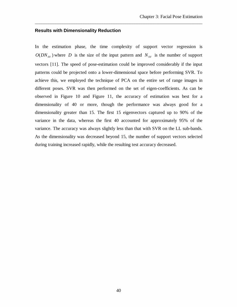
Chapter 3: Facial Pose Estimation ________________________________________________________________________
40
Results with Dimensionality Reduction
In the estimation phase, the time complexity of support vector regression is
)( SVDNO where D is the size of the input pattern and SVN is the number of support
vectors [11]. The speed of pose-estimation could be improved considerably if the input
patterns could be projected onto a lower-dimensional space before performing SVR. To
achieve this, we employed the technique of PCA on the entire set of range images in
different poses. SVR was then performed on the set of eigen-coefficients. As can be
observed in Figure 10 and Figure 11, the accuracy of estimation was best for a
dimensionality of 40 or more, though the performance was always good for a
dimensionality greater than 15. The first 15 eigenvectors captured up to 90% of the
variance in the data, whereas the first 40 accounted for approximately 95% of the
variance. The accuracy was always slightly less than that with SVR on the LL sub-bands.
As the dimensionality was decreased beyond 15, the number of support vectors selected
during training increased rapidly, while the resulting test accuracy decreased.
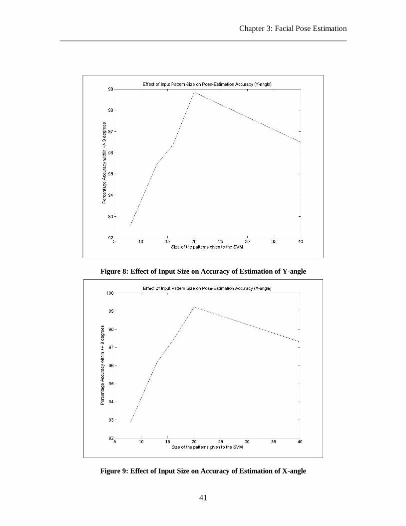
Chapter 3: Facial Pose Estimation ________________________________________________________________________
41
Figure 8: Effect of Input Size on Accuracy of Estimation of Y-angle
Figure 9: Effect of Input Size on Accuracy of Estimation of X-angle
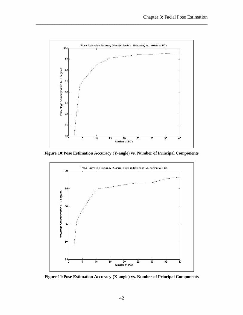
Chapter 3: Facial Pose Estimation ________________________________________________________________________
42
Figure 10:Pose Estimation Accuracy (Y-angle) vs. Number of Principal Components
Figure 11:Pose Estimation Accuracy (X-angle) vs. Number of Principal Components

Chapter 3: Facial Pose Estimation ________________________________________________________________________
43
(3.5) Discriminant Isometric Mapping
Discriminant Isometric Mapping is a new classification technique in pattern recognition
proposed in [15], where it has been applied for the purpose of face recognition. In this
thesis, it has been applied for the purpose of facial pose classification. A brief overview
of the theory of isometric mapping (ISOMAP) and discriminant isometric mapping is
presented in the following two sections.
(3.5.1) ISOMAP
ISOMAP is a nonlinear dimensionality reduction algorithm proposed by de Silva and
Tenenbaum [61]. Consider a densely sampled set of N points lying on a complex D-
dimensional manifold. The geometry of this manifold can be modeled well using the
geodesic distances between the N points, i.e. the distance between the points over the
surface of the manifold. The ISOMAP algorithm aims to obtain a matrix containing the
pair wise geodesic distances between all N points. First, the algorithm calculates the K
nearest Euclidean neighbors of each point (or alternatively, all Euclidian neighbors lying
within a radius of ε from each point on the manifold) and creates a neighborhood graph
in which each point represents a vertex. Each vertex is connected to its nearest neighbors
by edges weighted by the corresponding Euclidian distance. It is assumed that the
Euclidian distance is a good approximation of the geodesic distance between any points
and its nearest neighbors on the manifold. The geodesic distance between the “far-away”
points is calculated using Floyd’s algorithm [62] or Djikstra’s shortest path algorithm
[63] on the weighted neighborhood graph. The method of multidimensional scaling
(MDS) [64] is then applied to the matrix of geodesic distances in order to obtain a lower-
dimensional representation of the original manifold. While computing the lower-
dimensional projection, MDS minimizes the difference between the Euclidian distances
between points in the lower-dimensional space and the geodesic distances between the
corresponding points on the higher-dimensional manifold. The value of the parameter K
(or ε ) needs to be chosen by the user by trial and error. If the value of K is too large, the

Chapter 3: Facial Pose Estimation ________________________________________________________________________
44
geodesic distances may not be very well approximated due to short-circuiting. If it is too
small, it may lead to disconnected components in the graph. A good heuristic is to select
the smallest value of K that does not lead to any disconnected components in the graph.
Sometimes, for certain values of K , only a small fraction of points are disconnected from
the graph. In such cases, those points can “deleted” and ignored in further analysis [61].
(3.5.2) Discriminant ISOMAP
Consider N points, belonging to one of c different classes, all lying on a D-dimensional
manifold. Discriminant ISOMAP replaces the final MDS step of ISOMAP by Fisher’s
Linear Discriminant Analysis (LDA) [29]. Each point ix on the high-dimensional
manifold is treated as a N -dimensional vector iv of geodesic distances to other points.
LDA is then applied to this set of N -vectors. The between-class scatter matrix BS and
within-class scatter matrix WS are calculated as follows:
)')((
)')((
1 1
1
ijij
c
i
N
jW
ii
c
iiB
xxS
NS
µµ
µµµµ
−−=
−−=
� �
�
= =
=
Here, µ is the mean of all samples, iµ is the mean of all samples in the ‘ i’ th class, and
iN is the number of samples in the ‘ i’ th class. The projection matrix W is chosen to be
the one, which maximizes the ratio of the between-class scatter to the within-class scatter.
As per [29], W turns out to be the set of generalized eigenvectors of the between-class
and within-class scatter matrices corresponding to the m largest generalized eigenvalues.
As the number of classes is c , the number of non-zero generalized eigenvalues is only
1−c [29]. The lower-dimensional projection of the data point ix is given as ii Wvy = . In
this lower-dimensional space, the mean values of the samples in all the different classes
are separated as far as possible. Sometimes the matrix WS turns out to be singular. To

Chapter 3: Facial Pose Estimation ________________________________________________________________________
45
avoid this, one can use the techniques mentioned in [65] or add a small regularization
constant r to the diagonal elements of WS in order to make the eigenvalue problem more
stable.
(3.5.3) Motivation for Using Discriminant ISOMAP in Face Pose Estimation
Though ISOMAP has shown promise as a dimensionality reduction technique, it can be
sub-optimal from the point of view of a classification application [15]. Given an
ensemble of faces in different poses, one could make the assumption that the faces
represent points on a high dimensional manifold. Furthermore, it could be conjectured
that different faces in similar poses would lie closer together on the manifold. In other
words, the geodesic distance vectors for different faces in similar poses would bear an
inherent similarity with each other. ISOMAP projects these geodesic distance vectors
onto a lower dimensional space in a distance-preserving fashion. Thus, ISOMAP allows
similar points to cluster together in the lower dimensional space. This is however
assuming that the geodesic distance vectors have been accurately estimated. This
assumption in turn would be true if the number of data points sampled from the manifold
is large. The reason is that the graph would provide better and better approximate to the
“true” geodesic distance, as the number of points increases [61]. However, in case of very
high dimensional manifolds, it is difficult to obtain a very dense sampling of the manifold
and hence the number of points is small. Under such circumstances, the geodesic
distances obtained by applying Floyd’s or Djikstra’s algorithm may be inaccurate, and
hence ISOMAP may fail to appropriately project these points from the manifold onto the
lower-dimensional space. In problems such as face pose estimation, it is often difficult to
obtain a very large number of samples. Under such circumstances, the basic ISOMAP
algorithm would therefore be unsuitable. However discriminant ISOMAP would take into
account the distance between the centers of each different class and hence give better
classification results as reported in [15].

Chapter 3: Facial Pose Estimation ________________________________________________________________________
46
(3.5.4) Use of Discriminant Isometric Mapping for Pose Estimation
A set of different poses of a number of different individuals, labeled by the appropriate
pose angles, is first wavelet transformed. The LL sub-bands of these images at level three
are given to the discriminant isometric mapping routine to obtain a set of geodesic
distance vectors. These vectors are mapped onto a lower-dimensional space using FLD.
For testing, a facial scan, whose pose is to be determined, is wavelet transformed, and its
LL sub-band is obtained. The geodesic distance to the LL sub-bands of other training
images is determined. This geodesic distance vector is then mapped onto a lower-
dimensional space by projection onto the FLD matrix, giving a set of lower-dimensional
coordinates. The dimensionality of this space is equal to the number of classes (poses)
minus 1. A simple nearest-neighbor’s search in this space would yield the true pose of the
scan.
It should be noted that in comparison to support vector regression, discriminant isometric
mapping has some inherent limitations. It firstly requires the calculation of a pair-wise
geodesic distance matrix which is expensive in terms of both memory and time,
especially when the number of training samples is very high. At the time of actual pose-
estimation, all training samples need to be loaded into memory in order to obtain the
vector of geodesic distances. This further adds to the computational complexity of this
method.
(3.5.5) Results with Discriminant ISOMAP
The training data for pose estimation experiments with discriminant ISOMAP consisted
of all poses from 0 to 90 degrees around the Y-axis in steps of 3 degrees (i.e. 31 poses),
of 50 faces from the Freiburg database and 50 faces from the Notre Dame database. The
remaining faces were used for the purpose of testing. The original range images of the
different faces in different poses were pre-processed as described in section (3.4.6) and
decomposed by the level-3 discrete wavelet transform to yield 20 by 20 LL sub-bands.
The sub-bands were represented by 1 by 400 vector so that each image can be considered
as a point on a 400-dimensional manifold.

Chapter 3: Facial Pose Estimation ________________________________________________________________________
47
Discriminant ISOMAP was then applied to the pre-processed training set. The geodesic
distance matrix was calculated and each point was represented as a vector of geodesic
distances to other points. Geodesic distance vectors corresponding to faces in the same
pose were treated as members of one and the same class. As there are only 31 different
classes, the projection matrix W yielded by LDA will be a 30 by N matrix, i.e. these
vectors were mapped onto a lower-dimensional space using LDA. The dimensionality of
this space is 30, i.e. one less than the number of classes.
The pose estimation results in terms of percentage estimation accuracy within an absolute
error of 9 degrees versus the number of nearest Euclidian neighbors (i.e. K) varied from
10 to 40 have been shown in Figure 12 and Figure 13. The accuracy of the pose
estimation results is sensitive to the value of K . Figure 12 and Figure 13 show the
variation in the pose estimation accuracy with respect to K . The results shown are an
average of over 20 runs on both databases, choosing a different set of training and test
individuals each time. On an average, the best performance was observed for a value of K
= 25 for the Notre Dame database and K = 15 for the Freiburg database. However other
values of K between 10 and 50 still gave acceptable results. The accuracy of pose
estimation within +/- 9 degrees varied from 94% to 96% for the Notre Dame database
and 95% to 97% for the Freiburg database, across the 20 runs.
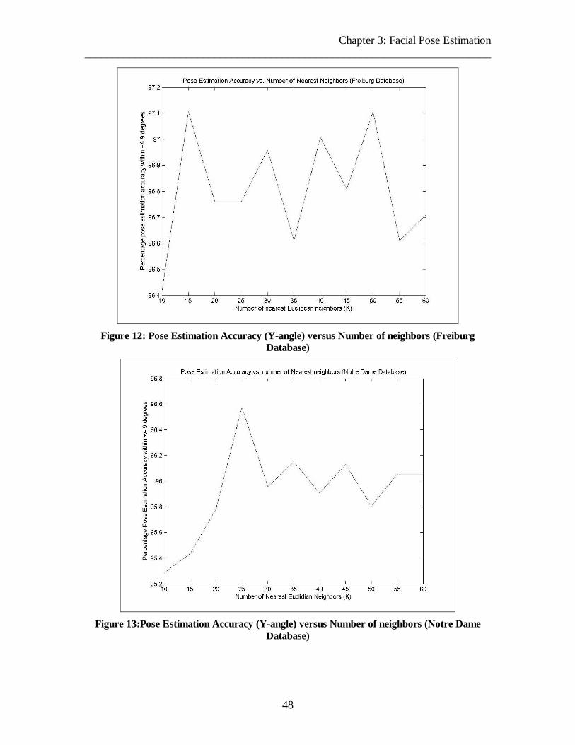
Chapter 3: Facial Pose Estimation ________________________________________________________________________
48
Figure 12: Pose Estimation Accuracy (Y-angle) versus Number of neighbors (Freiburg Database)
Figure 13:Pose Estimation Accuracy (Y-angle) versus Number of neighbors (Notre Dame Database)

Chapter 3: Facial Pose Estimation ________________________________________________________________________
49
(3.6) Conclusions
We conclude the following based on the observations given in this chapter:
1) The accuracy of pose estimation is the highest for an angular sampling of 3
degrees in both directions. Smaller sampling intervals do not improve the
accuracy, and only add to the computational cost.
2) Facial pose discrimination is highly reliable only for differences of 9 degrees in
either direction, as seen from the error histogram and tables. The original
assumption was that faces of different people in similar poses are more similar to
each other than poses of the same person in significantly different poses. The
results reinforce this belief.
3) Input sizes of 20 by 20 are sufficient for good pose estimation. Further reduction
in size causes depreciation in the ability to discriminate between poses that are 9
degrees apart. For larger input sizes, details specific to each individual begin
interfering with the SVM’s regression capabilities and there is a slight drop in the
pose estimation accuracy.
4) Dimensionality reduction with simple PCA speeds up the regression process with
a small decrease in accuracy.
5) Support Vector Regression is more suitable for pose-estimation than Discriminant
Isometric Mapping for reasons of computational efficiency. Also, the latter
requires all training images to be present in memory during the pose estimation
process in order to calculate the feature vector of the test pose. Moreover, the
results obtained upon using the latter are dependent upon the correct choice of the
number of nearest neighbors.

Chapter 4: 3D Face Recognition ________________________________________________________________________
50
Chapter Four: 3D Face Recognition
(4.1) Introduction
This chapter describes the methods implemented in the thesis for the purpose of face
recognition from 3D data. To perform recognition, an attempt is made to normalize the
probe image to a near frontal pose, where after a suitable similarity metric is employed to
compare the probe with a set of models from a database, so as to ascertain its correct
identity. Two methods are implemented for the purpose of normalization of a facial range
image to a frontal pose. The first is a feature-based technique, whereas the second follows
a global approach to align the facial surfaces using the Iterated Closest Point Algorithm
[17]. The disadvantages of both methods are discussed. The feature-based method is seen
to be highly susceptible to noise and results in a coarse normalization. The ICP algorithm
by itself is known to be prone to local minima [17]. Hence, a new hybrid method is
proposed, which first normalizes the facial image using feature-points, followed by a
more refined alignment using ICP. The hybrid method yields a better recognition rate
than either of the stand-alone techniques. Furthermore, an improved variant of ICP is
suggested. The proposed variant incorporates local surface properties such as local
moment invariants and surface curvature in order to improve the performance of ICP. It
also employs simple heuristics to discard outliers in the data. It is shown to outperform
the original algorithm. This chapter describes all of these techniques in detail. The
description of the individual algorithms is followed by a discussion of the experimental
results and a study of the effect of pose- and scale-variation on the recognition
performance.
It should be noted that the feature-based method used here requires the location of both
the eyes on the facial surface. Hence it would fail for facial poses with large yaw values
where one of the eyes is no more clearly visible. In such cases, for the first step of the
hybrid method, feature-based normalization could be replaced by the learning approach
using support vector regression, which has been described in detail in Chapter (3). This

Chapter 4: 3D Face Recognition ________________________________________________________________________
51
sort of a cascaded system using SVR as the first step followed by ICP is then capable of
matching a probe image in any pose across the view-sphere with the database consisting
of gallery images, for the purpose of view-invariant face recognition.
(4.2) Feature-Based Method
The aim of the face recognition system is to match the 3D scan of a face in any pose with
a set of models of different individuals (in frontal pose) stored in a database. For accurate
matching, it is important to normalize the images for geometric misalignments. This can
be done by detecting a few salient facial features and making use of the knowledge of
spatial relationships between them. These facial features include the two inner eye
corners and the nasal tip. The latter is located by making use of the fact that it is the
highest point on the range map. Similarly, analysis of the curvature map of the facial
range image facilitates the location of the eye concavities at the base (top) of the nose.
The inner eye corners lie within these concavities, but their exact location is difficult to
ascertain easily. Hence, all points within the left and right eye concavities are paired as
“candidate eye corners” . Anthropometric constraints are employed to prune the number
of possible candidate pairs. The facial range image is normalized for pose by performing
simple geometrical transformations, based on the position of the nasal tip and the position
of each such pair of “candidate eye corners” . The range image is appropriately cropped
and compared with the models stored in the database by means of a simple pixel-by-pixel
Euclidian distance function. All these steps are repeated for every possible pair of eye
corners. At the end, the model with the least distance value is taken as the correct identity
of the facial scan under test. This entire process is described in more detail in the ensuing
sections.
(4.2.1) Facial Feature Detection
We have implemented a method of facial feature detection that uses surface curvature
properties, adopting the approach that has been followed in [27] and [28]. This technique
of facial feature detection involves calculation of second derivatives (for curvature
computation). Despite the susceptibility of curvature to noise, we prefer it here to other

Chapter 4: 3D Face Recognition ________________________________________________________________________
52
existing feature detection methods such as eigen-templates [47]. This is owing to the
following reasons:
• The eigen-templates’ method requires extensive training, which involves accurate
manual marking of feature templates such as the eyes or the nose from a set of
facial range images.
• The eigen-templates’ method is extremely sensitive to facial scale changes, and
errors due to varying feature size or translation and head-rotation. The method
using curvatures is invariant to changes in scale, rotation and translation.
It is observed that there are distinct concavities at the eye corners near the base of the
nose on either side (i.e. the inner eye corners). A concavity occurs at regions where both
the mean curvature and the Gaussian curvature are greater than zero. Given a range
image ‘S’ , we can calculate the mean curvature H and the Gaussian curvature K at each
point as follows:
)5.1()^1(2
)1(2)1(22
22
yx
xxyxyyxyyx
SS
SSSSSSSH
++++−+
=
2)^1( 22
2
yx
xyyyxx
SS
SSSK
++−
=
Here xS and yS are the first derivatives of S in the X and Y directions at that particular
point, and xxS , yyS , xyS represent the corresponding second derivatives in the
appropriate directions.
Consider the depth map of a face as shown in Figure 14. Using the above formulae, we
can calculate the mean and Gaussian curvature at every pixel in the depth map and then
detect concave regions in the face. Owing to factors such as noise and minor depressions
on the facial surface, several small concave regions are detected all over the face (see
Figure 15). To detect the eyes, the following algorithm is adopted:

Chapter 4: 3D Face Recognition ________________________________________________________________________
53
1. Use a simple connected components analysis to label all coherent concave
regions. (See Figure 16).
2. Discard all concave regions smaller than say T pixels (T is chosen to be 5), as
these regions most likely correspond to noise. Concave regions such as those at
the inner eye corners, the nostrils and the mouth corners are much larger.
3. Discard all concave regions below the nasal tip. See Figure 17. Of the remaining
regions, select the two that are closest to the nasal tip and lying on either side of
the nasal ridge. This finally leads to two approximately symmetric concavities.
4. The inner eye corners lie within these two concave regions. In order to find exact
eye corners, pairs are formed between every point in the left concavity and every
point in the right concavity. Anthropometric constraints are taken into
consideration so as to prune the number of “candidate eye corner pairs” . These
constraints are as follows:
• The distance 1d between the left eye corner and the nasal tip, and the
distance 2d between the right eye corner and the nasal tip, should differ
by a very small value less than a threshold 1τ .
• Let 1θ be the angle between the nasal line and the line joining the nasal tip
and the left inner eye corner. Let 2θ be defined similarly for the right eye.
The angles 1θ and 2θ should have a difference below a certain threshold
2τ .
The location of the exact eye corners is performed simultaneously with recognition as
described in the following section. (The values of 1τ and 2τ are chosen to be 0.01).
(4.2.2) Facial Normalization and Recognition
Next, the face is normalized and recognition is performed during the normalization
process itself, as described in the sequence of steps given below:
• The line joining a pair of candidate eye corners is aligned with the X-axis using a
simple 3D rotation matrix.

Chapter 4: 3D Face Recognition ________________________________________________________________________
54
• The nasal ridge is located by first detecting the nasal tip (using the fact that it is
the highest point in the nasal region) and then employing a least-squares line
fitting algorithm to predict the position of the nasal base (between the eyebrows).
The nasal ridge is aligned with the Y-axis using a 3D transformation, and the face
is given a reverse tilt of about 20 degrees to align it to a completely frontal view.
• Then, the translation normalization is applied. All facial points are interpolated
onto a 150 by 150 grid taking into account aspect ratio and using the required zero
padding. The entire range image is translated such that the nasal tip always
coincides with the central pixel. If the Z value at the nasal tip is denoted as p, then
the value of 100-p is added to all facial points so as to normalize for translation in
the Z direction. (See Figure 18).
• Using the locations of the eye corners and the nasal tip in addition to knowledge
of facial anthropometry, a cropping function is applied to automatically discard
the portions of the range image that lie outside the facial contour. (See Figure 19).
• The normalized image is compared (in terms of pixel by pixel Euclidian distance)
with every gallery image from the database and the distances are recorded.
• The above five steps are repeated for every single candidate pair of points from
the left and right eye concavities. The candidate pair which gives the least
Euclidian distance to any of the models is chosen to be the correct pair of inner
eye corners, ideally giving the correct facial identity as well as the exact pose.
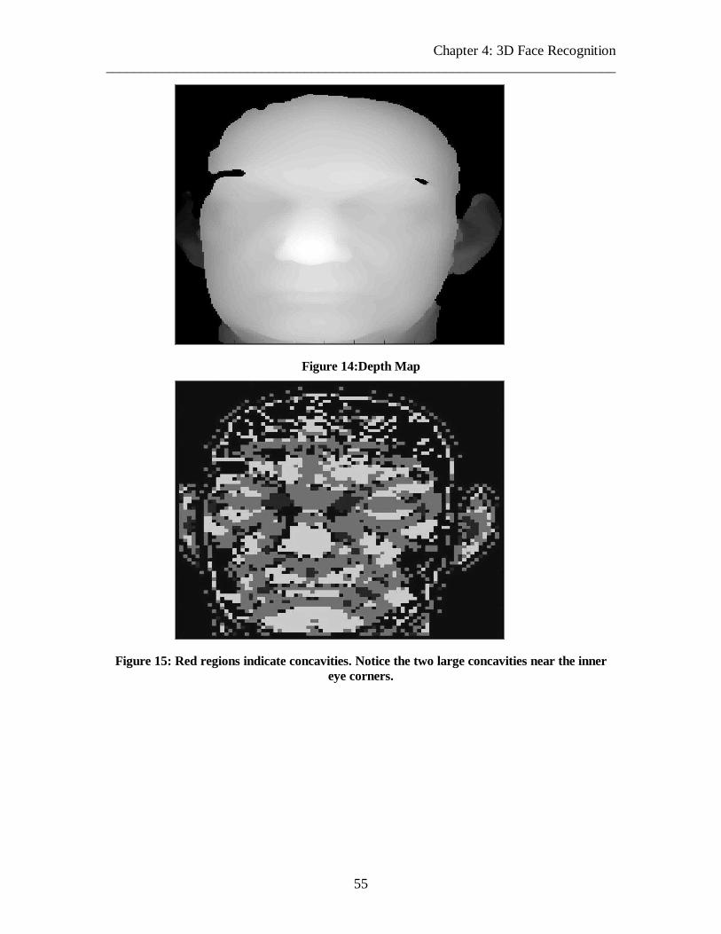
Chapter 4: 3D Face Recognition ________________________________________________________________________
55
Figure 14:Depth Map
Figure 15: Red regions indicate concavities. Notice the two large concavities near the inner eye corners.
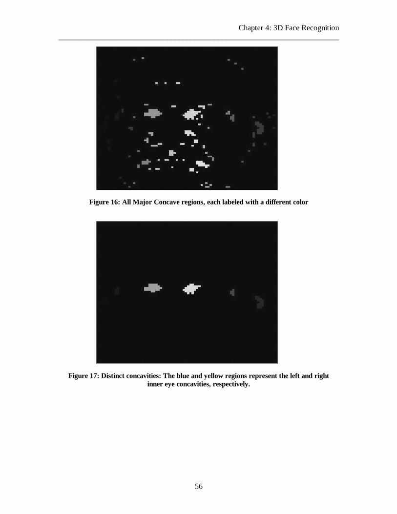
Chapter 4: 3D Face Recognition ________________________________________________________________________
56
Figure 16: All Major Concave regions, each labeled with a different color
Figure 17: Distinct concavities: The blue and yellow regions represent the left and right inner eye concavities, respectively.
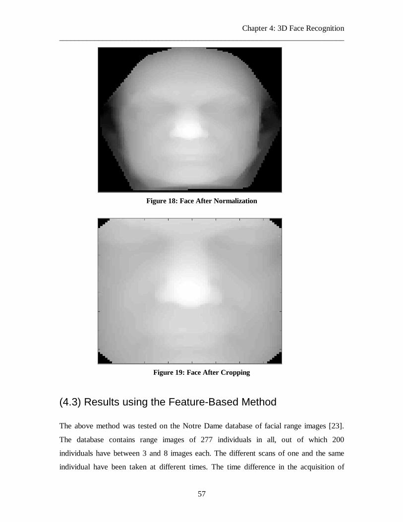
Chapter 4: 3D Face Recognition ________________________________________________________________________
57
Figure 18: Face After Normalization
Figure 19: Face After Cropping
(4.3) Results using the Feature-Based Method
The above method was tested on the Notre Dame database of facial range images [23].
The database contains range images of 277 individuals in all, out of which 200
individuals have between 3 and 8 images each. The different scans of one and the same
individual have been taken at different times. The time difference in the acquisition of

Chapter 4: 3D Face Recognition ________________________________________________________________________
58
these images ranges from 6 up to 13 weeks [23]. All images in this database were taken
by means of a Minolta Vivid 900 range scanner [69]. There are 77 individuals having
only one range image, and they have not been considered in the experiments conducted
as part of this thesis. For the other 200 individuals, exactly one of the different range
images per person is chosen as the gallery or training image. The gallery images are all in
frontal pose. The remaining images of each person act as probes or testing images. Given
a probe, it was matched to each of the 200 models by means of a pixel-by-pixel Euclidian
distance as explained in the previous section. The model that gave the least distance was
chosen to be the true identity of the probe.
It was observed that the facial feature detection method largely failed for images from
this database. The eye-concavities were always located accurately. However the angle
made by the eye-line with the X-axis was miscalculated due to noise present in the depth
values. As a result the Euclidian matches failed to give correct identity results. In fact, the
eye lines as detected by this method in different range images of one and the same
individual were found to be inconsistent. The resulting face recognition accuracy
considering the 200 individuals was only 58%. The conclusion that can be drawn is that
individual feature points are difficult to locate accurately and that the resulting
normalization is highly coarse, which leads to very poor performance in terms of
recognition rates.
(4.4) Global Approach
Three-dimensional face (or object) recognition is known to be extremely sensitive to the
slightest changes in pose. In order to develop a robust recognition system, it is of utmost
importance that the facial surfaces are registered as accurately as possible. As seen from
the previous section, feature based methods yield a very coarse alignment. For the
purpose of refining the alignment thus obtained, a variant of the Iterated Closest Point
Algorithm (which was proposed by Besl and McKay [17]) is applied. Basically, ICP is a
global matching algorithm and does not rely on the detection of just a few fiducial points,
consequently being more advantageous in terms of robustness to noise. Another major
advantage of ICP is that it does not require any prior training on a database, unlike

Chapter 4: 3D Face Recognition ________________________________________________________________________
59
methods such as PCA [19]. However, as will be discussed in sub-section (4.3.2), ICP has
a couple of disadvantages. A set of modifications is proposed so as to be able to
overcome these drawbacks, giving rise to a variant of ICP, which is experimentally
shown to perform better than the original, in section (4.5). A two-step cascade algorithm
is proposed and its results have also been discussed further on.
(4.4.1) Iterated Closest Point Algorithm
The basic ICP algorithm has been briefly described in the literature review in Chapter (2).
A more detailed description is presented here for the sake of completeness. Assume a
model M of a face containing MN points. Consider a probe scan D containing DN
points, which we have to register with the model. The basic steps of the ICP algorithm
are given below:
1. For each point in the scan D , find the closest point in the scan M . This
establishes a rough correspondence between the points in scan D and scan M .
2. Using the above correspondence, estimate the relative motion between the two
scans by using a least-squares technique such as singular value decomposition.
For this, the points of scan M and scan D are centered by subtracting their
respective centroids, cm and cd . Let the centered set of points be denoted as m
and d . The covariance matrix K is then calculated from these points. Using
singular value decomposition, the covariance matrix K is expressed in the form
USVK = where S is a matrix of singular values, V is a right orthogonal matrix
and U contains the orthogonal bases. The rotation between M and D can then be
expressed as 'VUR = and the translation between the two frames is then
computed as cdRcmT *−= .
3. The motion ),( TR calculated in step (2) is applied to the data set D .
4. Using the knowledge of the correspondence established in step (1), the mean
squared error is calculated between the points of M and D .
5. Steps (1) to (4) are repeated until a convergence criterion is satisfied. The
convergence criterion chosen in our implementation is that the change in error
between two consecutive iterations should be less than a certain tolerance value

Chapter 4: 3D Face Recognition ________________________________________________________________________
60
ζ and that this condition should be satisfied for a set of at least 8 successive pairs
of iterations.
It should be noted that the motion estimated in every iteration is applied only to scan D ,
whereas scan M is always kept fixed. Scan M is often called as the “model” , whereas
scan D is called the “data” . Besl and McKay have proved that ICP converges to a local
minimum, and that the mean-squared error between the two surfaces being registered
undergoes a monotonic decrease at successive iterations [17]. It is also observed that the
decrease in error between two consecutive iterations is very large initially, where after it
begins to drop significantly [17].
(4.4.2) Variant of ICP
The basic iterated closest point algorithm is known to suffer from a number of
drawbacks, as follows:
1. The algorithm assumes that for every point in the scan D, there necessarily exists
a corresponding point in the scan M. This may not be strictly true for significant
out of plane rotations of the facial scan, which leads to occlusion of certain facial
features, or in case of noise or artifacts in the scanned data. Such points are called
outliers. For instance, if a probe image has a high out-of-plane rotation, it may
contain points at the edge of the face, which do not correspond to any particular
point on the surface of the model (which is in frontal pose).
2. The algorithm is prone to getting stuck in a local minimum if the two datasets
being aligned are not in approximate alignment initially [17].
3. The algorithm ascertains correspondence solely based on the criterion of
Euclidian distance between the X, Y and Z coordinates of the points, without
taking into consideration of local shape information.
To improve on the above drawbacks, we have proposed a variant of the ICP algorithm, in
which we have incorporated the following changes:

Chapter 4: 3D Face Recognition ________________________________________________________________________
61
• Determining the Corresponding Points: Traditionally, the closest points are
determined by finding the Euclidian distances between points in the two scans,
making use of just the X, Y and Z coordinates. However, one can easily exploit
the fact that ICP is trivially extensible to points in a higher-dimensional space. In
order to improve the correspondence established in each iteration, some properties
of the neighborhood surrounding each point in the two 3D scans being registered
can also be taken into account. These properties include the following:
1. Mean Curvature
2. Gaussian curvature
3. The three local second order moment-invariants that were proposed by
Sadjadi and Hall [75].
In other words, every 3D point is effectively being treated as a point in 8
dimensions given as ),,,,,,,( 35241321 JJJKHzyxP ααααα= , where ),( KH
represents the mean and Gaussian curvature, respectively, ),,( 321 JJJ represents
the three second-order moment-invariants in 3D, and α indicates the weight given
to each surface property. The mean and Gaussian curvatures are calculated using
the formulae mentioned in Section (4.2.1). The second order moment invariants
are given as follows [75]:
2011200
2101020
21100020111011100020202003
0112
1012
1102
0020200022000202002
0020202001
2 µµµµµµµµµµµµµµµµµµµµµ
µµµ
−−−+=
−−−++=
++=
J
J
J
Here pqrµ denotes the centralized moment in 3D given as
),,()()()( zyxzzyyxx rqppqr ρµ −−−= �����
where ),,( zyxρ is a piecewise continuous function that has a value of 1 over a
spherical neighborhood around the central point ),,( zyx and 0 elsewhere.
The value of α is chosen to be equal to the reciprocal of the difference between
the maximum and minimum values of that particular property in the model scan.

Chapter 4: 3D Face Recognition ________________________________________________________________________
62
It should be noted that surface curvature and the moment-invariants are all
rotationally invariant. Hence, it is not necessary to compute these feature values at
the data points in each successive iteration. The idea of using curvature values
besides the point coordinates for ascertaining correspondence was implemented in
prior work on surface registration by Feldmar and Ayache [71].
• Eliminating outliers: Outliers, that is, point pairs that are incorrectly detected as
being in correspondence, can cause incorrect registration. To eliminate as many
outliers as possible, the following heuristic is used. Let the distances between
each point in the data and its closest point in the model be represented as the array
Dist . While computing the motion between the two scans, we can ignore all
those point pairs for which the distance value is greater than σ5.2 . Here σ is the
standard deviation of the values in Dist calculated using robust methods that
make use of the median of the distances (denoted as med ) which is always less
sensitive to noise than the mean [72]. The exact relationship between the median
of the distances and the value of σ is given as med4826.1=σ . This heuristic has
been suggested in an ICP variant put forth by Zhang [69] and Masuda [72].
• Duplicate correspondences: It is always possible that one and the same point
belonging to the model happens to lie closest to more than one point in the scan
D. Under such circumstances, only the point pair with the least distance is
considered and the remaining point pairs are discarded while calculating the
motion using SVD.
(4.4.3) Improving Algorithm Speed
The computationally most expensive step in each iteration of the ICP algorithm and all its
variants is the one involving determination of the corresponding point pairs5. If the model
and the data contain MN and DN points respectively, then the time complexity of the
5 It was observed that a single registration between a pair of range-images took between 6 to 14 seconds on a Pentium III, 700 MHz.

Chapter 4: 3D Face Recognition ________________________________________________________________________
63
correspondence calculation is )( DM NNO . This is prohibitively expensive even for
moderately sized 3D scans, if a naïve search method is used. A much better alternative is
to make use of an efficient geometric data structure such as the k-d tree [73], as has been
suggested by Zhang [69]. The k-d tree is a generic data structure where k denotes the
dimensionality of the data stored in each leaf of the tree (in our case k = 8). K-d trees are
known to be very efficient for dimensions of less than 20. A single k-d tree is constructed
out of each model in the database. The time for the construction of the k-d tree is
))log(( MM NKNO and the average time for a single nearest neighbor query is
))(log( MNO . This leads to an average speedup of )log( M
M
N
N per iteration. In this thesis,
we have implemented the k-d tree algorithm outlined by Bentley [74].
Another heuristic can be adopted in order to further speed up the process, ensuring no
loss of accuracy whatsoever. It can be observed that in the initial stages of the ICP
algorithm, the established correspondence is quite coarse. Under such circumstances, we
carry out the initial registrations on a down-sampled version of the model and data. In our
implementation, both scans have been down-sampled by a factor of 2 in the X and Y
directions. As the change in mean squared error obtained over two consecutive iterations
drops below a certain pre-defined threshold (chosen to be 0.1), we switch to the scans
with the original resolution. During the initial iterations, the search time is improved by a
factor of more than 4 per iteration, owing to the fact that down-sampled images are being
used. Two separate k-d trees are created in this case, one for the down-sampled model
and the other for the model with full resolution.
A third interesting strategy for improving the speed of registration between two surfaces
is to neglect those points on the probe that lie on planar regions. We say that a point lies
on a planar region of the surface if the value of the curvature )( 22
21 κκκ += sqrt at that
point is less than a small threshold (say 0.02), where 1κ and 2κ are the two principal
curvatures. Thus registration is performed using only those points that have curvature
values above a certain threshold. Typically, around 40% of the facial points are seen to

Chapter 4: 3D Face Recognition ________________________________________________________________________
64
lie in planar regions. If these points are not considered (during the computation of the
motion parameters by SVD), we need to perform a smaller number of closest point
searches in each iteration, resulting in speed-up of nearly 1.5 times as compared to the
original algorithm. The motivation for not using the planar points is that they do not
represent any particular distinct feature on the surface of the face. Incorporation of this
strategy did not cause any reduction in the recognition rate.
(4.5) Experimental Results using the Global Approach
All experiments for face recognition were carried out on images from the Notre Dame
Database [23], as described in section (4.3). The probe images were first coarsely
normalized using the facial features method described in section (4.2) and cropped. The
model images were in frontal pose as described before and similarly cropped. The
cropping was essential to avoid interference due to different hairstyles of one and the
same individual. Sample images of the cropped models and their respective probes from
the Notre Dame database are shown in Figure 20 and Figure 21. Next, the ICP algorithm
was applied in order to register the probe one by one with each of the gallery images
stored in the database. The experimental results were recorded. The experiments were
repeated once again, employing the proposed ICP variant, instead of the original version
of ICP. The final recognition results obtained were 83.87% with ICP and 91.5% with the
modified version of ICP as shown in Table 3.
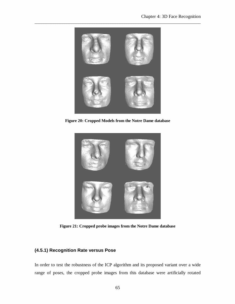
Chapter 4: 3D Face Recognition ________________________________________________________________________
65
Figure 20: Cropped Models from the Notre Dame database
Figure 21: Cropped probe images from the Notre Dame database
(4.5.1) Recognition Rate versus Pose
In order to test the robustness of the ICP algorithm and its proposed variant over a wide
range of poses, the cropped probe images from this database were artificially rotated

Chapter 4: 3D Face Recognition ________________________________________________________________________
66
through angles of 20, 30, 40 and 50 degrees around the Y-axis, and projected onto the
front viewing plane using the Z-buffer algorithm [74]. These rotated probe images were
then used as input to the recognition system. The images were directly given as input to
the ICP algorithm for registration with the model faces (which are in frontal pose). Such
an experiment facilitated the measurement of the maximum angle over which the ICP
algorithm and its proposed variant produced acceptable results. Table 3 shows the effect
of these rotations on the overall recognition rate. In all cases, the suggested ICP variant
outperformed the original algorithm proposed by Besl and McKay [17] in terms of the
obtained recognition rate. These results have also been compared to those obtained using
a surface registration algorithm called LMICP proposed by Fitzgibbon [76]. This
algorithm is similar to ICP except that it makes use of the iterative Levenberg-Marquardt
optimization algorithm [77] for computation of the motion between the two scans. The
ICP variant suggested in this thesis outperforms LMICP as well. Moreover, the suggested
ICP variant shows a fairly graceful degradation in performance as the angle of rotation
increases. LMICP [76] performs slightly better than ICP [17] in terms of the obtained
recognition rate. However, it is much slower owing to the fact that it requires several
closest point computations in each iteration for the purpose of calculating the partial
derivatives required in each step of the Levenberg-Marquardt optimization [76].
(4.5.2) The Two-step Cascade
From Table 3 it is observed that both ICP as well as the proposed variant are susceptible
to local minima, owing to which the recognition rate suffers as the pose difference
between the probes and the models increases, though the degradation in performance
with the ICP variant is much less. This forms a major motivating factor to use the feature-
based step before applying the ICP variant forming a two-step cascade. Employment of
such a scheme increases the recognition rate by a few percent. The overall recognition
rate is dependent upon the accuracy of both the stages in the cascade. The rate will suffer
considerably if the feature-based method predicts the pose erroneously. However it was
observed that for probes with yaw rotation beyond 20 degrees, employment of the
feature-based initialization helped increase the performance figures on an average up to

Chapter 4: 3D Face Recognition ________________________________________________________________________
67
81.5% when ICP was used as the second step, and up to 86% when the ICP variant was
used for refinement of normalization. These results are shown in Table 4.
It should be noted that the pose estimation module using support vector regression
(described in chapter (3)) could also be used as the first step, replacing the feature-based
method. This is because the pose estimation technique using support vector regression is
able to predict the facial pose very reliably within an error of 9 degrees. Using this
learning-based approach as the first stage has several advantages over using the feature-
based stage. We know that the latter requires the detection of both eye-concavities in
order to perform coarse normalization. For yaw changes beyond 50 degrees, one of the
two eyes is no more visible. For such cases, the feature-based method cannot be used,
whereas the method using support vector machines will still predict the approximate pose
of the facial scan. When such a learning scheme is incorporated, we now obtain a face
recognition system that performs robustly over a very wide range of facial poses. As has
been shown in Table 5, one can observe that the recognition rate in this case is high even
from probe images at extreme profile views.

Chapter 4: 3D Face Recognition ________________________________________________________________________
68
Face Recognition Rates (Percentage) Angle of rotation of probes
(Around Y-axis) ICP ICP Variant LMICP
+/- 10 degrees 83.8 91.5 84.2
+/- 20 degrees 80.5 90 80.5
+/- 30 degrees 78.5 86.6 78.4
+/- 40 degrees 76.3 84 76.4
+/- 50 degrees 73.5 81.5 74.5
Table 3: Recognition Rates with ICP, ICP Variant and LMICP
Face Recognition Rates
(Percentage)
Angle of rotation of probes
(Around Y-axis)
Features +
ICP
Features +
ICP Variant
+/- 10 degrees 83.8 91.5
+/- 20 degrees 82.5 90.5
+/- 30 degrees 81.5 88.3
+/- 40 degrees 78.5 86
+/- 50 degrees 77 84.5
Table 4: Recognition Rates with ICP and the ICP Variants after applying the feature-based method as an initial step
Face Recognition Rates (Percentage) Angle of rotation of probes
(Around Y-axis) SVR + ICP SVR + ICP Variant
+/- 10 degrees 83.8 91.5
Angles between +/- 20 to +/- 50 degrees 81.16 88
Angles between +/- 50 to +/- 90 degrees 80.5 87
Table 5: Recognition rates with ICP and ICP variant after applying SVR as the initial step

Chapter 4: 3D Face Recognition ________________________________________________________________________
69
(4.5.3) Dealing with Missing Points
Facial scans with large yaw rotations invariably contain “missing points” as nearly half
the face is occluded from the scanner. After applying the coarse registration in the first
step (using either method) on scans with large yaw, one can observe triangulation
artifacts in the near-frontal image thus obtained. In order to prevent such points from
hampering an optimal registration, we can first detect the nasal ridge and discard the
points that originally belonged to the “more occluded” side of the face. Thereafter, we
make use of the fact that the human face is symmetric6 about the nasal ridge and register
just half the probe image with the models in the database. Moreover, we can consider just
one half of each model scan from the database (which further improves the registration
efficiency).
(4.5.4) Error Histograms
The recognition rates obtained by employing all the above-mentioned iterative
registration algorithms are dependent upon the residual error values obtained at
convergence. These values are analyzed below for the proposed ICP variant. Histograms
are plotted for the residual error values when the surfaces being registered belong to one
and the same person, and also when they belong to different people. The histograms are
plotted in Figure 22 and Figure 23, while Figure 24 shows both histograms overlaid on
top of one another, for easier comparison. As expected, the residual error values are much
less when the facial surfaces being registered belonged to one and the same person as
compared to those obtained for different people. The difference between the average
error values recorded for the same and different people is an entire order of magnitude. In
the former case, the error values are concentrated between 0.1 and 0.8, whereas in the
latter case they lie mostly between 1 and 6.
6 Though the symmetry assumption may not strictly hold true in reality, we contend that this is a reasonable assumption to make, for all practical purposes.
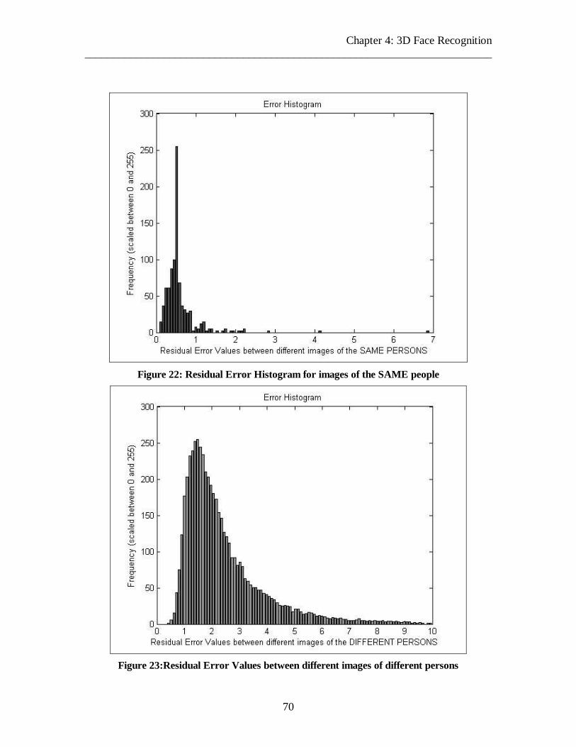
Chapter 4: 3D Face Recognition ________________________________________________________________________
70
Figure 22: Residual Error Histogram for images of the SAME people
Figure 23:Residual Error Values between different images of different persons
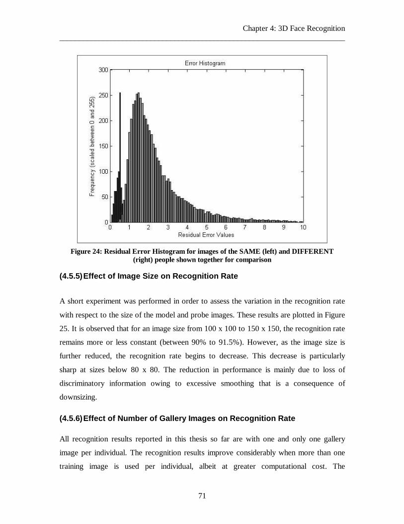
Chapter 4: 3D Face Recognition ________________________________________________________________________
71
Figure 24: Residual Error Histogram for images of the SAME (left) and DIFFERENT (right) people shown together for comparison
(4.5.5) Effect of Image Size on Recognition Rate
A short experiment was performed in order to assess the variation in the recognition rate
with respect to the size of the model and probe images. These results are plotted in Figure
25. It is observed that for an image size from 100 x 100 to 150 x 150, the recognition rate
remains more or less constant (between 90% to 91.5%). However, as the image size is
further reduced, the recognition rate begins to decrease. This decrease is particularly
sharp at sizes below 80 x 80. The reduction in performance is mainly due to loss of
discriminatory information owing to excessive smoothing that is a consequence of
downsizing.
(4.5.6) Effect of Number of Gallery Images on Recognition Rate All recognition results reported in this thesis so far are with one and only one gallery
image per individual. The recognition results improve considerably when more than one
training image is used per individual, albeit at greater computational cost. The

Chapter 4: 3D Face Recognition ________________________________________________________________________
72
computational cost increases because each time, the probe image has to be registered one-
by-one with multiple gallery images per individual. The variation in recognition rate
versus the number of training images per individual is shown in Figure 26. The reader is
reminded that these training images were taken on different occasions within a 13-week
period.
(4.5.7) Implications for Expression Invariance
The ICP algorithm and the suggested variant assume that the two surfaces being matched
differ only by a rigid transformation. However, human facial expressions are a non-rigid
transformation and can cause considerable changes in appearance. Under such cases,
these algorithms may fail to register the two facial surfaces optimally, causing reduction
in recognition rates. There are two possible ways to overcome this problem. The first is to
modify the error function for computing the transformation between the facial surfaces,
so as to accommodate non-rigid changes. Such an approach would require knowledge of
the facial musculature and movements of the various regions of the face in order to arrive
at a robust function that would be able to simulate realistic facial expressions.
In this thesis, we adopt a much simpler approach. One can observe that certain regions of
the face are more “deformable” than others. For instance, the topology of areas such as
the cheeks or the lips undergoes far greater change with normal facial expressions, than
regions such as the nose, the eyebrow-ridges, the forehead or the chin. Therefore, by
assigning a lower importance (or “weight” ) to the facial points around the mouth or the
cheeks, one can induce a degree of expression invariance in the algorithm. (Such
modifications have been suggested in previous research on 3D face recognition, for
instance by Gordon in [27] and Lee and Milios in [26]). In other words, while calculating
the mean squared residual error at the end of each iteration, the errors for the set of points
that lie in the non-rigid areas of the probe scan are weighted by a factor λ that is less than
one. Thus, the formula for the calculation of the mean squared error between two scans
can be written as follows:

Chapter 4: 3D Face Recognition ________________________________________________________________________
73
2_
1
2_
1
)()( i
NONRIGIDN
iii
RIGIDN
ii PMPMMSE −+−= ��
==λ
Here iM and iP refer to corresponding points on the model and probe scans respectively.
The value of λ in the above expression should always be between zero and one. If it is
equal to 1, it is the same as giving the same weight to all areas of the face. If λ is equal
to 0, it is the same as totally discarding non-rigid areas of the face.
In order to fully automate the process of discarding non-rigid regions, we employ a facial
feature detector to detect the location of the nose, eyes or the mouth (see Figure 28). We
then apply simple heuristics to identify the deformable regions of the face and finally
perform the registration.
Experiments for testing this technique were performed on the entire Notre Dame
database. The value of λ was varied from 0 to 1 in steps of 0.1 and recognition rate was
measured for each different value of this parameter. It was observed that the recognition
rate actually dropped from 91.5% to around 89.4% if the non-rigid regions were totally
discarded (i.e. λ was set to 0). This was owing to the fact that some discriminatory
information was lost when totally discarding areas such as the cheek and the mouth. The
best recognition rate (92.3%) was attained when λ was set to a value of 0.3. We would
additionally like to mention that the value of λ might be dependent on the actual database
on which the experiments were performed. However, owing to the fact that the quantity
of data is very large, we would conjecture that this value is stable for the general case as
well. For all values of this parameter less than or equal to 0.5, it was observed that
different scans of one and the same individual carrying significantly different facial
expressions were always registered to lower residual error values than before the
employment of this heuristic. Figure 27 shows a pair of scans of the same person with
discernibly different facial expression. Figure 28 shows the lines of demarcation between
the rigid and non-rigid regions of the face.
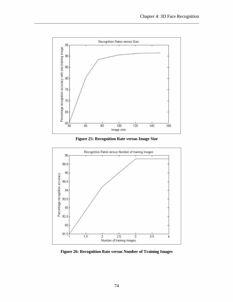
Chapter 4: 3D Face Recognition ________________________________________________________________________
74
Figure 25: Recognition Rate versus Image Size
Figure 26: Recognition Rate versus Number of Training Images
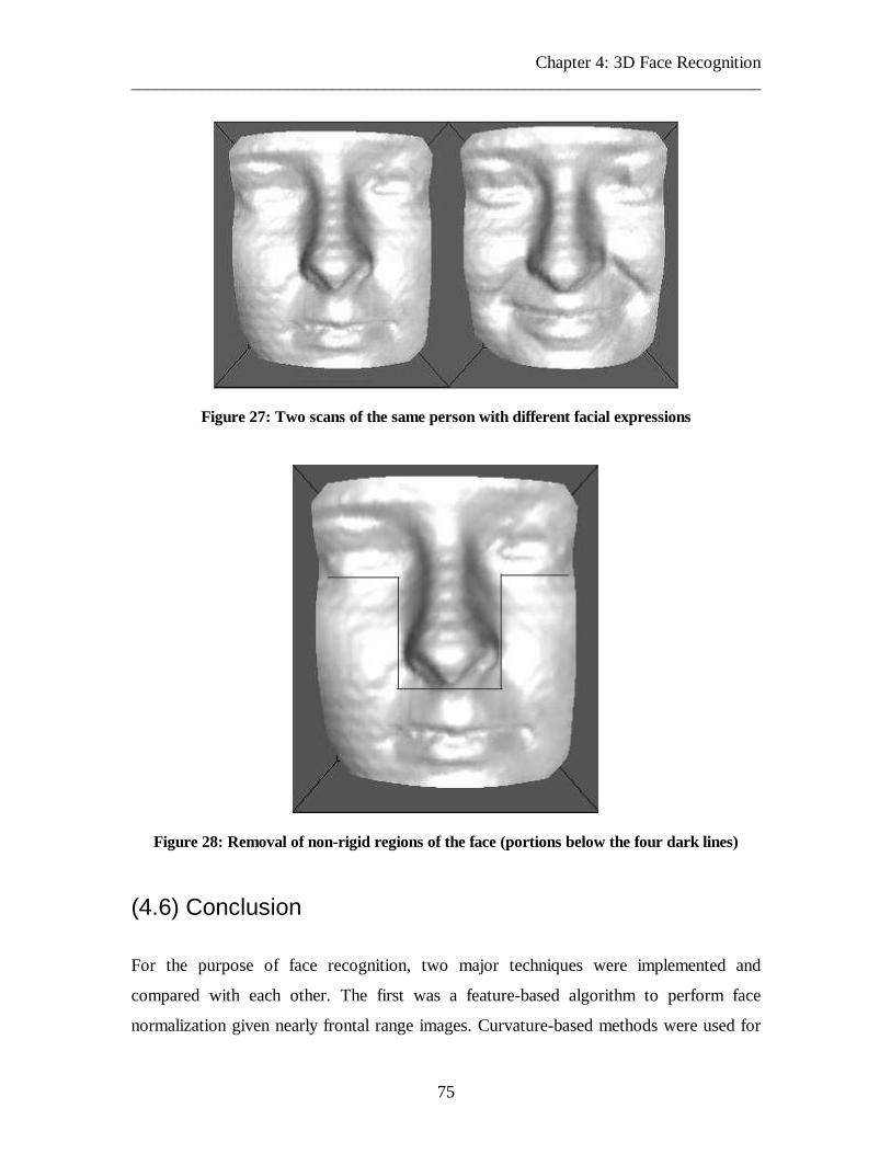
Chapter 4: 3D Face Recognition ________________________________________________________________________
75
Figure 27: Two scans of the same person with different facial expressions
Figure 28: Removal of non-rigid regions of the face (portions below the four dark lines)
(4.6) Conclusion
For the purpose of face recognition, two major techniques were implemented and
compared with each other. The first was a feature-based algorithm to perform face
normalization given nearly frontal range images. Curvature-based methods were used for

Chapter 4: 3D Face Recognition ________________________________________________________________________
76
facial feature localization. It was observed that feature-based methods are too sensitive to
noise and small artifacts that are common in range data, consequently giving poor
recognition results.
Instead, a global iterative approach has been adopted after an initial coarse normalization
(using the feature-based alignment), which significantly improved the recognition rates
over a wide range of poses. The global algorithm is a modification of the well-known ICP
algorithm [17]. The modified version of the algorithm uses local surface properties for
establishing the correspondence between points on the two surfaces being registered. It
also employs methods to reject outliers. The proposed variant outperforms existing
algorithms such as ICP [17] and LMICP [76] over a wide range of poses.
To improve registration speed, a geometric data structure called the k-d tree has been
used as suggested in [69]. Additionally, a simple heuristic has been incorporated, which
involves using down-sampled images during the initial iterations of the registration
process, until the change in residual error in successive iterations falls below a specified
threshold. Employment of this heuristic does not cause any reduction in recognition
accuracy.
The recognition results obtained were tested over a wide range of poses of the probe
images. Experimental results are also reported, showing the effect of variation in image
size and variation in the number of training images per individual on the overall
recognition rate. A simple method for incorporating some amount of expression
invariance in the face recognition algorithm has been discussed. Using this approach, an
increase in recognition rate up to 92.3% was observed.
In addition to all these experiments, we have quantified the effect of increase in pose
difference between the probe and gallery images on the face recognition rate. We observe
that the feature-based method cannot be used for recognition from extreme profile views
of the face. Alternatively, we propose the use of support vector regression (described in
detail in Chapter (3)) as the initial step, which makes our system robust to a very wide

Chapter 4: 3D Face Recognition ________________________________________________________________________
77
range of poses, yielding good recognition rates even from extreme profile views of the
face.

Chapter 5: Conclusions ________________________________________________________________________
78
Chapter Five: Conclusions and Future Work
In this section, we present the conclusions of the thesis. We first briefly summarize its
accomplishments, and further present a brief comparison regarding the use of range
versus texture data from the point of view of face recognition. Lastly, we mention some
of the limitations of the present study and outline directions for future work.
Thesis Summary
This thesis presents a learning approach using support vector machines to predict the
approximate pose (in terms of angles of rotation around two axes) of any face from its 3D
scan. Experimental results relating range image size to the accuracy of pose prediction
have been discussed. Similarly, results of the effect of dimensionality reduction on the
pose estimation performance have been given.
A two-stage facial normalization technique has been proposed and implemented, with a
view to aligning the 3D scan of any face to a near-frontal view. The normalization
process consists of an initial stage consisting of alignment based on location of three
salient feature points, or based on the pose angles predicted using the support vector
machine. The second stage in the normalization process refines the angle estimate in
order to bring the 3D scan as close to a completely frontal view as possible. For this, a
robust variant of the Iterated Closest Point algorithm is proposed and employed. The
algorithm uses local surface properties to improve the correspondences during the ICP
iterations. It also incorporates simple heuristics to improve upon computational
efficiency. A simple way to induce a degree of expression invariance to the registration
process has also been put forth. The entire iterative registration process yields residual
error values, which are used as metrics to test the similarity between the 3D scan under
test and the facial models (one each per individual) stored in a database. Unlike several
existing 3D face recognition systems, the technique in the thesis is robust over a wide

Chapter 5: Conclusions ________________________________________________________________________
79
range of poses spanning the complete view-sphere. If support vector regression is used as
the initial stage of the normalization cascade, our system performs well in terms of
recognition, even from extreme profile views of the face. Additionally, our approach has
been tested on a large database in which the gallery and probe images have been acquired
at significantly different times [23].
Range versus Texture Data for Face Recognition
The thesis completely ignores texture information, in any form, for face recognition. The
results with range data are encouraging given the complexity of the database the
experiments were performed on. However, it is also interesting to examine the merits and
demerits of using range data compared to texture data for the purpose of face recognition.
Firstly, range data are largely invariant to incident illumination given that the scanner
captures the 3D geometry of the face with a relatively uniform and constant light source..
Thus one would expect 3D face recognition rates to be more stable than conventional 2D
methods even in outdoor lighting. Secondly, the presence of 3D information facilitates
proper pose normalization since a correction for out-of-plane rotation is now possible.
This is not as easily possible using intensity images, as they are a projection of a 3D
object onto a plane. Accurate pose correction in 2D would require multiple training or
gallery images, each one sampled at a different pose, whereas a single range-image is
sufficient in the 3D case. Despite these inherent advantages, 3D face recognition systems
have limitations, often imposed by the quality of the 3D sensor. For instance, the outputs
of 3D sensors are often noisy, containing spikes or holes or triangulation artifacts in
certain regions of the face, such as the eyes, eyebrows, beards or moustaches. These
artifacts are uncommon with 2D sensors. In the case of 3D sensors such as stereo
cameras, a major issue is the effect of illumination conditions on the quality of the output
of the sensor [81]. Secondly, from the point of view of human perception, a range image
offers far less discriminatory information than an intensity image (regardless of the
incident illumination). These issues may be the reasons why 3D face recognition rates are
not as high as those reported on 2D data. The trend in face recognition has shifted
towards multi-modality wherein both range and texture data of the face are used in

Chapter 5: Conclusions ________________________________________________________________________
80
association with fused classifiers [20], [23]. The results using multiple data inputs have
been shown to be clearly superior to those with only range or only texture. However, the
issue of correction for illumination effects on the texture data before employment of the
combined classifiers needs to be sufficiently elaborated.
Scope for Future Work
The present study has some limitations, such as the high computational cost of the
recognition method, the problem of expression invariance over a wide range of emotions
and the effect of occlusions. In the following paragraphs, we briefly discuss these issues
and point out ways and means for further improvement.
(1) Efficiency Considerations:
Despite the several different methods employed to improve the computational costs (see
section (4.4.3)), ICP remains an inefficient algorithm, especially from the point of view
of a real-time recognition application. This is because every probe image has to be
matched to each one of the models stored in the database. Each of these matches is
iterative and the total time required is therefore extremely high. One potential solution
could be to locate salient feature points on all range images and use a rigid transformation
(SVD for instance) to perform range-image alignment. This would reduce the iterative
ICP procedure to a single-step procedure. However, as seen in the thesis, accurate
location of the feature points is a non-trivial problem despite the incorporation of
anthropometric heuristics. Similar results have been reported in [28] and [40].
Development of robust algorithms to solve this problem would be a challenging direction
for future research. Combining both range and texture information might prove beneficial
for improving the accuracy of feature point detectors. Recently, a new technique has been
developed for detecting points of interest in color (and gray-scale) images using local
symmetries [84]. The salient points detected by this method are shown to be more stable
and “distinctive” than just corners or edges [84]. Extension of such a technique to range

Chapter 5: Conclusions ________________________________________________________________________
81
data (or a combination of range and texture data) would be an interesting experiment
from the point of view of robust facial feature-point detection.
(2) Expression Invariance:
Future work can include improvement of the largely empirical method in section (4.5.8)
for inducing invariance to facial expression. An interesting way to address the problem of
facial expressions would be to explore the possibility of the application of non-rigid
matching techniques, such as thin plate splines (TPS’s) [79]. TPS’s are a class of non-
rigid mapping algorithms, which have the desirable property of splitting any given
deformation into an affine and a non-affine component. Algorithms such as those
proposed in [78] have incorporated TPS’s within the ICP framework to estimate non-
rigid deformation and correspondence simultaneously, and have been applied to solve the
problem of non-rigid registration of brain MRI of different subjects. These algorithms
could be extended to optimally register faces of one and the same individual with
different facial expression. An important point to be noted here is that such a method
would have to be modified suitably so as to reliably distinguish between non-rigid shape
changes due to identity and non-rigid shape changes due to facial expression.
The second way to solve the problem of variations in facial geometry due to expression
would be the employment of Kimmel’s method of canonical signatures derived from
geodesic distances, which are known to be invariant to all isometric deformations [34].
This method has the added advantage of computational efficiency, as it is a non-iterative
technique.
For either approach, it would be interesting to test the algorithm for 3D face recognition
purposes by checking its effectiveness across different types of emotions (such as smiles,
frowns or larger facial distortions due to surprise or anger, or facial deformations during
speech). However, such a study would require collecting a suitable 3D database
containing different range images of one and the same individual with several different

Chapter 5: Conclusions ________________________________________________________________________
82
types of facial expressions or generation of such a database from range images by
employing techniques of facial animation such as [82], [83].
(3) Effect of occlusions:
Another interesting extension to the thesis would be to explore to what extent the
occlusion of some portions of the face such as the eyes or nose (due to spectacles or
scarves) affects the quality of facial surface registration, and to incorporate recognition
methods that would be provably robust to large occlusions of features in the face, using a
parts-based approach such as non-negative matrix factorization [80].
Concluding Remarks
In this thesis we have presented a 3D face recognition system using a two-step pose
normalization technique and analyzed its merits and limitations. Based on the discussions
in this chapter, we conclude that 3D face recognition (either stand-alone or in conjunction
with 2D recognition techniques) has the potential of becoming an important method of
biometric authentication in the real world. However a significant amount of research
would be required on the improvement of 3D sensing technology and on development of
more efficacious algorithms along the aforementioned lines, in order to create a system
that is capable of recognizing the identity of individuals in a manner that is robust,
efficient (in terms of real-time computation) and fully automatic.

Citations ________________________________________________________________________
83
Citations
[1] “The Iris Recognition Homepage”, http://www.iris-recognition.org/
[2] D. Maltoni, D. Maio, A. Jain and S. Prabhakar, “Handbook of Fingerprint
Recognition” , Springer Verlag, 2003.
[3] “Canesta Inc.” , http://www.canesta.com/sensors.htm/
[4] R. Zhang, P. Tsai, J. Cryer and M. Shah, “Shape from Shading: A Survey” , IEEE
Transactions on Pattern Analysis and Machine Intelligence, Vol. 21, No. 8, pp.
690-706, 1999.
[5] J. Aloimonos, “Shape from Texture” , Biological Cybernetics, Vol. 58, pp. 345-
360, 1988.
[6] T. Huang and A. Netravali, “Motion and Structure from Feature Correspondence:
A Review”, Proceedings of the IEEE, Vol. 82, No. 2, pp. 252-268, 1994.
[7] S. Nayar, K. Ikeuchi and T. Kanade, “Shape from Interreflections” , International
Journal of Computer Vision, Vol. 6, No. 3, pp. 173-195, 1991.
[8] S. Seitz, “An Overview of Passive Vision Techniques” , Carnegie Mellon
University, http://www.cs.cmu.edu/~seitz, 1999.
[9] T. Fromherz, “Shape from Multiple Cues for 3D-Enhanced Face Recognition” ,
PhD Thesis, University of Zurich, 1996.
[10] J. Daugman, “Face and Gesture Recognition: Overview”, IEEE Transactions on
Pattern Analysis and Machine Intelligence, Vol. 19. No. 7, pp. 675-676, 1997.
[11] C. Burges, “A Tutorial on Support Vector Machines for Pattern Recognition” ,
Data Mining and Knowledge Discovery, Vol. 2, No. 2, pp. 121-167, 1998.
[12] V. Vapnik, “Statistical Learning Theory” , John Wiley and Sons, New York, 1998.
[13] A. Schmola and A. Scholkopf, “A Tutorial on Support Vector Regression” ,
NeuroCOLT2 Technical Report NC2-TR-1998-030, 1998.
[14] K. Bennet and C. Campbell, “Support Vector Machines: Hype or Hallelujah?”
SIGKDD Explorations, Vol. 2, No.2, pp. 1-13, 2000.
[15] M. Yang, “Discriminant Isometric Mapping for Face Recognition” , Lecture Notes
in Computer Science, Springer Verlag.

Citations ________________________________________________________________________
84
[16] J. Sherrah, S. Gong and E. Ong, “Face Distributions in Similarity Space Under
Varying Head Pose”, Image and Vision Computing, Vol. 19, pp. 807-819, 2001.
[17] P. Besl and N. McKay, “A Method for Registration of 3D Shapes” , IEEE
Transactions on Pattern Analysis and Machine Intelligence, Vol. 14, No. 2, pp.
239-256, 1992.
[18] M. Turk and A. Pentland, “Eigenfaces for Recognition” , Journal of Cognitive
Neuroscience, Vol. 3, pp. 71-86, 1994.
[19] C. Hesher, A. Srivastava and G. Erlebacher, “Principal Component Analysis of
Range Images for Facial Recognition” , Proceedings of CISST, Las Vegas, June
2002.
[20] F. Tsalakanidou, D. Tzovaras and M. Strintzis, “Use of Depth and Color
Eigenfaces for Face Recognition” , Pattern Recognition Letters, Vol. 24, pp. 1427-
1435, 2003.
[21] B. Achermann, X. Jiang and H. Bunke, “Face Recognition using Range Images” ,
Proceedings of the International Conference on Virtual Systems and Multimedia,
pp. 129-136, 1997.
[22] P. Jonathan Phillips, H. Moon, S. Rizvi and P. Rauss, “The FERET Evaluation
Methodology for Face-Recognition Algorithms”, IEEE Transactions on Pattern
Analysis and Machine Intelligence, Vol. 22, No. 10, pp. 1090-1104, October 2000.
[23] K. Chang, K. Bowyer and P. Flynn, “Face Recognition Using 2D and 3D Facial
Data” , 2003 Multimodal User Authentication Workshop, pp. 25-32, December
2003.
[24] H. Tanaka, M. Ikeda and H. Chiaki, “Curvature-Based Face Surface Recognition
Using Spherical Correlation Principal Directions for Curved Object Recognition” ,
Proceedings of the 3rd International Conference on Automated Face and Gesture
Recognition, pp. 372-377, 1998.
[25] Fisher and Lee, “Correlation Coefficients for Random Variables on a Unit Sphere
or Hypersphere” , Biometrica, No. 73, pp. 159-164, 1986.
[26] J. Lee and E. Milios, “Matching Range Images for Human Faces” , Proceedings of
the International Conference on Computer Vision, pp. 722-726, 1990.

Citations ________________________________________________________________________
85
[27] G. Gordon, “Face Recognition Based on Depth Maps and Surface Curvature” ,
Geometric Methods in Computer Vision: SPIE, pp. 1-12, 1991.
[28] A. Moreno, A. Sanchez, J. Velez and F. Diaz, “Face Recognition using 3D
Surface-extracted Descriptors” , Proceedings of Irish Machine Vision and Image
Processing Conference, September 2003.
[29] R. Duda and P. Hart, “Pattern Classification and Scene Analysis” , New York:
Wiley and Sons, 1973.
[30] Y. Lee, K. Park, J. Shim and T. Yi, “3D Face Recognition using Statistical
Multiple Features for Local Depth Information” , Proceedings of the 16th
International Conference on Vision Interface, June 2003.
[31] C. Chua and R. Jarvis. “Point Signatures: A New Representation For 3D Object
Recognition” , International Journal Computer Vision, Vol. 25, No. 1, pp. 63-85,
1997.
[32] C. Chua, F. Han, Y. Ho, “3D Human Face Recognition Using Point Signature” ,
Proceedings of the 4th IEEE International Conference on Automatic Face and
Gesture Recognition, pp. 233-239, 2000.
[33] Y. Wang, C. Chua and Y. Ho, “Facial Feature Detection and Face Recognition
from 2D and 3D Images” , Pattern Recognition Letters, Vol. 23, pp. 1191-1202,
2002.
[34] A. Elad and R. Kimmel, “On Bending Invariant Signatures for Surfaces” , IEEE
Transactions on Pattern Analysis and Machine Intelligence, Vol. 25, No. 10, pp.
1285-1295, October 2003.
[35] A. Bronstein, M. Bronstein and R. Kimmel, “Expression Invariant 3D Face
Recognition” , Proceedings of the Audio and Video Based Biometric Person
Authentication, pp. 62-69, 2003.
[36] A. Tal, M. Elad and S. Ar, “Content-based Retrieval of VRML Based Objects –
an Iterative and Interactive Approach”, EG Multimedia, 97, 2001.
[37] J. Kruskal and M. Wish, “Multidimensional Scaling” , Sage, 1978.
[38] Y. Chen and G. Medioni, “Object Modeling by Registration of Multiple Range
Images” , Proceedings of the International Conference on Robotics and
Automation, 1991.

Citations ________________________________________________________________________
86
[39] X. Lu, D. Colbry and A. Jain, “Three Dimensional Model-Based Face
Recognition” , Proceedings of the International Conference on Pattern
Recognition, 2004.
[40] X. Lu, D. Colbry and A. Jain, “Matching 2.5D Scans for Face Recognition” ,
Proceedings of the International Conference on Biometric Authentication (ICBA),
2004.
[41] V. Blanz and T. Vetter, “A Morphable Model for the Synthesis of 3D Faces” ,
Proceedings of SIGGRAPH, pp. 353-360, July 1999.
[42] S. Romdhani, V. Blanz and T. Vetter, “Face Identification by Fitting a 3D
Morphable Model using Linear Shape and Texture Error Functions” , Proceedings
of the European Conference on Computer Vision, pp. 3-19, 2002.
[43] T. Sim, S. Baker and M. Bsat, “The CMU Pose, Illumination and Expression
(PIE) Database of Human Faces” , Technical Report CMU-R1-TR-01-02, CMU
2000.
[44] P. Phillips, P. Grother, R. Michaels, D. Blackburn, E. Tabassi and J. Bone,
“FRVT 2002: A Overview and Summary” , March 2003.
[45] N. Krüger, M. Pötzsch, C. von der Malsburg, “Determination of Face Position and
Pose with a learned Representation based on labeled Graphs” , Image and Vision
Computing, Vol. 15, No. 10, pp. 741-748, 1997.
[46] K. Hattori, S. Matsumori and Y. Sato, “Estimating Pose of Human Face Based on
Symmetry Plane using Range and Intensity Image”, Proceedings of the
International Conference on Pattern Recognition, pp. 1183-1187, 1998.
[47] A. Pentland, B. Moghaddam and T. Starner, “View-based and Modular
Eigenspaces” , Proceedings of the International Conference on Computer Vision
and Pattern Recognition, 1994.
[48] B. Moghaddam and A. Pentland, “Probabilistic Visual Learning for Object
Representation” , IEEE Transactions on Pattern Analysis and Machine
Intelligence, Vol. 19, No. 7, pp. 696-710, 1997.
[49] H. Murase and S. K. Nayar, “Visual learning and recognition of 3-D objects from
appearance”, International Journal of Computer Vision, Vol. 14, pp. 5-24, 1995.
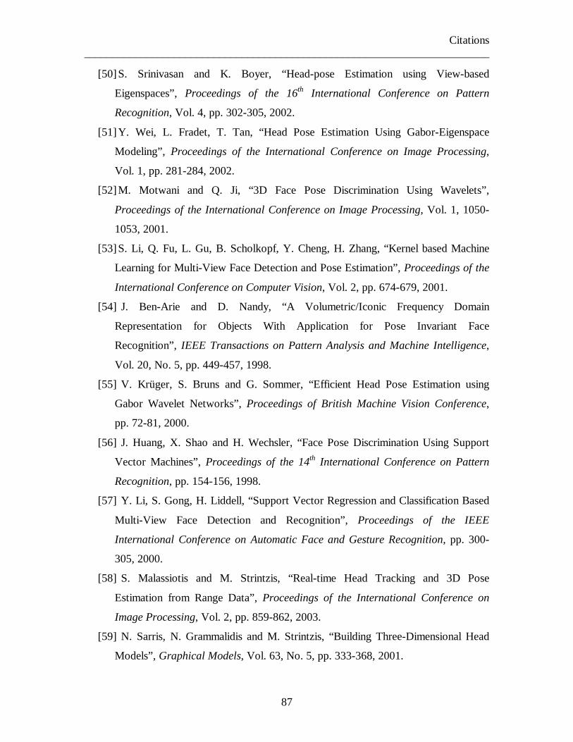
Citations ________________________________________________________________________
87
[50] S. Srinivasan and K. Boyer, “Head-pose Estimation using View-based
Eigenspaces” , Proceedings of the 16th International Conference on Pattern
Recognition, Vol. 4, pp. 302-305, 2002.
[51] Y. Wei, L. Fradet, T. Tan, “Head Pose Estimation Using Gabor-Eigenspace
Modeling” , Proceedings of the International Conference on Image Processing,
Vol. 1, pp. 281-284, 2002.
[52] M. Motwani and Q. Ji, “3D Face Pose Discrimination Using Wavelets” ,
Proceedings of the International Conference on Image Processing, Vol. 1, 1050-
1053, 2001.
[53] S. Li, Q. Fu, L. Gu, B. Scholkopf, Y. Cheng, H. Zhang, “Kernel based Machine
Learning for Multi-View Face Detection and Pose Estimation” , Proceedings of the
International Conference on Computer Vision, Vol. 2, pp. 674-679, 2001.
[54] J. Ben-Arie and D. Nandy, “A Volumetric/Iconic Frequency Domain
Representation for Objects With Application for Pose Invariant Face
Recognition” , IEEE Transactions on Pattern Analysis and Machine Intelligence,
Vol. 20, No. 5, pp. 449-457, 1998.
[55] V. Krüger, S. Bruns and G. Sommer, “Efficient Head Pose Estimation using
Gabor Wavelet Networks” , Proceedings of British Machine Vision Conference,
pp. 72-81, 2000.
[56] J. Huang, X. Shao and H. Wechsler, “Face Pose Discrimination Using Support
Vector Machines” , Proceedings of the 14th International Conference on Pattern
Recognition, pp. 154-156, 1998.
[57] Y. Li, S. Gong, H. Liddell, “Support Vector Regression and Classification Based
Multi-View Face Detection and Recognition” , Proceedings of the IEEE
International Conference on Automatic Face and Gesture Recognition, pp. 300-
305, 2000.
[58] S. Malassiotis and M. Strintzis, “Real-time Head Tracking and 3D Pose
Estimation from Range Data” , Proceedings of the International Conference on
Image Processing, Vol. 2, pp. 859-862, 2003.
[59] N. Sarris, N. Grammalidis and M. Strintzis, “Building Three-Dimensional Head
Models” , Graphical Models, Vol. 63, No. 5, pp. 333-368, 2001.

Citations ________________________________________________________________________
88
[60] S. Mallat, “A Theory for Multiresolution Signal Decomposition: the Wavelet
Representation” , IEEE Transactions on Pattern Analysis and Machine
Intelligence, Vol. 11, No. 7, pp. 674-693, 1989.
[61] J. Tenenbaum, Vin de Silva, J. Langford, “A Global Geometric Framework for
Nonlinear Dimensionality Reduction” , Science, Vol. 290, pp. 2319-2323, 2000.
[62] T. Cormen, C. Leiserson, and R. Rivest, “Introduction to Algorithms”, The MIT
Press and McGraw-Hill Book Company, 1989.
[63] E. Dijkstra, “A Note on Two Problems in Connection with Graphs” , Numerische
Mathematik, Vol. 1, pp. 269-271, 1959.
[64] F. Young and R. Hamer, “Multidimensional Scaling: History, Theory and
Applications” , Erlbaum Assoc., New York, 1987.
[65] P. Belhumeur, J. Hespanha and D. Kriegman, “Eigenfaces vs. Fisherfaces:
Recognition Using Class-Specific Linear Projection” , IEEE Transactions on
Pattern Analysis and Machine Intelligence, pp. 711-720, 1997.
[66] N. Amenta, S. Choi and R. Kolluri, “The Power Crust” , Sixth ACM Symposium
on Solid Modeling and Applications, pp. 249-260, 2001.
[67] E. Catmull, “A Sub-Division Algorithm for Computer Display of Curved
Surfaces” , PhD Thesis, Department of Computer Science, University of Utah, Salt
Lake City, USA.
[68] C. Chang and C. Lin, “LIBSVM: a Library for Support Vector Machines” ,
http://www.csie.ntu.edu.tw/~cjlin/libsvm/, 2001.
[69] “Minolta Vivid 900 Range Scanner” ,
http://ph.konicaminolta.com.hk/eng/industrial/3d.htm
[70] Z. Zhang, “On Local Matching of Free-form Curves” , Proceedings of the British
Machine Vision Conference, pp.347-356, 1992.
[71] J. Feldmar and N. Ayache, “Rigid, Affine and Locally Affine Registration of
Free-form Surfaces” , International Journal of Computer Vision, Vol. 18, No.2, pp.
99-119, 1996.
[72] T. Masuda, K. Sakaue and N. Yokoya, “Registration and Integration of Multiple
Range Images for 3D Model Construction” , Proceedings of the International
Conference on Computer Vision and Pattern Recognition, pp. 879-883, 1996.

Citations ________________________________________________________________________
89
[73] F. Preparata and M. Shamos, “Computational Geometry” , Springer Verlag, 1985.
[74] J. Bentley, “K-d Trees for Semidynamic Point Sets” , Proceedings of the 6th
Annual Symposium on Computational Geometry, pp. 187-197, 1990.
[75] F. A. Sadjadi and E. L Hall, “Three-dimensional Moment Invariants” , IEEE
Transactions on Pattern Analysis and Machine Intelligence, Vol. 2, No. 2, pp.
127-136, March 1980.
[76] A. Fitzgibbon, “Robust Registration of 2D and 3D Point Sets” , Proceedings of the
British Machine Vision Conference, pp. 411-420, 2001.
[77] W. Press, S.Teukolsky, W. Fetterling and B. Flannery, “Numerical Recipes in C:
The Art of Scientific Computing” , Cambridge University Press, Cambridge, 1992.
[78] H. Chui and A. Rangarajan, “A New Algorithm for Non-rigid Point Matching” ,
IEEE Conference on Computer Vision and Pattern Recognition, Vol. 2, pp. 44-51,
2000.
[79] F. Bookstein, “Principal Warps: Thin-plate splines and the decomposition of
deformations” , IEEE Transactions on Pattern Analysis and Machine Intelligence,
Vol. 11, No. 6, pp. 567-585, June 1989.
[80] D. Guillamet and J. Vitria, “Classifying Faces with Non-negative Matrix
Factorization” , Proceedings of the 5th Catalan Conference for Artificial
Intelligence, pp. 24-31, 2002.
[81] W. Boehler and A. Marbs, “3D Scanning Instruments” , International Workshop
on Scanning for Cultural Heritage Recording, Corfu, Greece, 2002.
[82] F. Parkes and K. Waters, “Computer Facial Animation” , A. K. Peters Ltd., 1996.
[83] S. Platt and N. Badler, “Animating Facial Expression” , ACM Computer
Graphics, Vol. 15, August 1981.
[84] G. Heidemann, “Focus-of-attention from Local Color Symmetries” , IEEE
Transactions on Pattern Analysis and Machine Intelligence, Vol. 26, No. 7, pp.
817-830, July 2004.