Embed Size (px)
Citation preview
Face Recognition:
Two-Dimensional and
Three-Dimensional Techniques
Thomas David Heseltine BSc. Hons.
The University of York
Department of Computer Science
- For the Qualification of PhD. -
- September 2005 -
Abstract
- 2 -
ABSTRACT
We explore the field of automated face recognition. Beginning with a survey of
existing methods applied to two-dimensional (2D) and three-dimensional (3D) face
data, we focus on subspace techniques, investigating the use of image pre-processing
applied as a preliminary step in order to reduce error rates. We implement the eigenface
and Fisherface methods of face recognition, computing False Acceptance Rates (FAR)
and False Rejection Rates (FRR) on a standard test set of images that pose typical
difficulties for recognition. Applying a range of image processing techniques we
demonstrate that performance is highly dependant on the type of pre-processing used
and that Equal Error Rates (EER) of the eigenface and Fisherface methods can be
reduced from 25.5% to 20.4% and 20.1% to 17.8% respectively, using our own
specialised methods of image processing. However, with error rates still too high for
use in many proposed applications we identify the use of 3D face models as a potential
solution to the problems associated with lighting conditions and head orientation.
Adapting the appearance-based subspace methods previously examined, for application
to 3D face surfaces, introducing the necessary orientation normalisation and format
conversion procedures, we show that low error rates can be achieved using surface
shape alone, despite variations in head orientation and expression. In addition, these
techniques are invariant to lighting conditions as no colour or texture information is
used in the recognition process.
We introduce a 3D face database providing 3D texture mapped face models, as well as
2D images captured at the same instant. This database facilitates a direct comparison of
3D and 2D techniques, which has not previously been possible. Contrasting the range
of face recognition systems we explore methods of combining multiple systems in order
to exploit the advantage of several methods in a single unified system. Various methods
of system combination are tested, including combination by dimensional accumulation,
elimination and genetic selection. This research leads to an innovative multi-subspace
face recognition method capable of combining 2D and 3D data, producing state-of-the-
art error rates, with a clear advantage over single subspace systems: The lowest EER
achieved using 2D, 3D and 2D Projection methods are 9.55%, 10.41% and 7.86%
respectively, yet multi-subspace combination reduces this error down to 4.50% on the
same test data.

Abstract
- 3 -
Continuing research into the use of 3D face models we develop an additional novel
method of recognition, based on the correlation of isoradius contour signal ensembles,
which possesses significant advantages over other methods in that orientation
normalisation is encapsulated within the recognition process and hence not required as a
preliminary alignment procedure. It is also able to simultaneously utilise information
from many data modalities, such as colour, texture, shape and temperature, giving great
potential as an aid to facial orientation normalisation or as a separate 3D object
recognition technique in its own right.

Table of Content
- 4 -
TABLE OF CONTENT
ABSTRACT 2
TABLE OF CONTENT 4
L IST OF FIGURES 9
L IST OF TABLES 18
ACKNOWLEDGMENTS 19
AUTHOR ’S DECLARATION 20
1 INTRODUCTION 21
1.1 FACE RECOGNITION AS A BIOMETRIC 22
1.2 THESIS RATIONALE 26
1.3 RESEARCH GOALS 29
2 THESIS STRUCTURE 31
3 LITERATURE REVIEW 35
3.1 2D APPROACHES 35
3.1.1 APPEARANCE-BASED SUBSPACE METHODS 41
3.2 3D APPROACHES 48
3.3 RECOGNITION DIFFICULTIES 56
3.4 HUMAN FACIAL PERCEPTION 57
3.5 SUMMARY OF PERFORMANCE 60
4 TWO-DIMENSIONAL FACE RECOGNITION 62
4.1 FEATURE LOCALIZATION 64
4.2 THE DIRECT CORRELATION APPROACH 66
4.2.1 VERIFICATION TESTS 67
4.2.2 RESULTS 72
4.3 THE EIGENFACE APPROACH 74
4.3.1 PRELIMINARY EXPERIMENTATION 76
4.3.2 IMAGE RESOLUTION AND CROP REGION INVESTIGATION 78
4.3.3 IMAGE PRE-PROCESSING RESULTS 82

Table of Content
- 5 -
4.3.4 CONCLUSION 85
4.4 THE FISHERFACE APPROACH 87
4.5 IMAGE PRE-PROCESSING TECHNIQUES 89
4.5.1 COLOUR NORMALISATION METHODS 90
4.5.2 STATISTICAL METHODS 93
4.5.3 CONVOLUTION METHODS 96
4.5.4 METHOD COMBINATIONS 99
4.6 IMPROVING AND COMPARING 2D FACE RECOGNITION 102
4.6.1 TEST PROCEDURE 102
4.6.2 CONCLUSION 104
5 THREE-DIMENSIONAL FACE RECOGNITION 107
5.1 3D FACE MODELS 108
5.1.1 DATA ACQUISITION 108
5.1.2 CAPTURE CONDITIONS 109
5.1.3 3D FACE DATA 111
5.2 ORIENTATION NORMALISATION 115
5.2.1 NOSE TIP LOCALISATION 116
5.2.2 ROLL CORRECTION 118
5.2.3 TILT CORRECTION 119
5.2.4 PAN CORRECTION 119
5.2.5 FINE TUNING AND BACK-CHECKING 120
5.3 3D SURFACE REPRESENTATIONS 122
5.3.1 DEPTH MAP GENERATION 122
5.3.2 3D SURFACE PROCESSING 124
5.4 DIRECT CORRELATION 129
5.5 THE EIGENSURFACE APPROACH 132
5.5.1 VERIFICATION OF FACIAL SURFACES 132
5.5.2 EVALUATION PROCEDURE 133
5.5.3 RESULTS 134
5.5.4 CONCLUSION 136
5.6 THE FISHERSURFACE APPROACH 138
5.6.1 EVALUATION PROCEDURE 140

Table of Content
- 6 -
5.6.2 RESULTS 141
5.6.3 CONCLUSION 142
5.7 IRAD F ACE CONTOURS 144
5.7.1 PREVIOUS WORK 145
5.7.2 THE IRAD CONTOUR REPRESENTATION 147
5.7.3 ISORADIUS CONTOUR GENERATION 147
5.7.4 SIGNAL EXTRACTION 151
5.7.5 IRAD COMPARISON 155
5.7.6 DEALING WITH NOISE 159
5.7.7 IRAD VARIANCE DUE TO FACIAL EXPRESSION 161
5.7.8 RESULTS 162
5.7.9 SUMMARY 165
6 2D-3D FACE RECOGNITION 167
6.1 RECOGNITION USING 3D TEXTURE MAP PROJECTIONS 168
7 COMBINING METHODS OF FACE RECOGNITION 171
7.1 COMBINING 2D FACE RECOGNITION 172
7.1.1 THE EIGENFACE AND FISHERFACE METHODS 173
7.1.2 TEST DATA 174
7.1.3 ANALYSIS OF FACE RECOGNITION SYSTEMS 175
7.1.4 COMBINING SYSTEMS 181
7.1.5 THE TEST PROCEDURE 183
7.1.6 RESULTS 184
7.1.7 CONCLUSION 189
7.2 COMBINING 3D FACE RECOGNITION 193
7.2.1 TEST DATA 194
7.2.2 SURFACE SPACE ANALYSIS 194
7.2.3 COMBINING SYSTEMS 196
7.2.4 THE TEST PROCEDURE 199
7.2.5 RESULTS 200
7.2.6 CONCLUSION 203

Table of Content
- 7 -
7.3 METHODS OF COMBINATION OPTIMISATION 205
7.3.1 COMBINATION BY DIMENSIONAL ELIMINATION 206
7.3.2 COMBINATION BY DIMENSIONAL ACCUMULATION 207
7.3.3 COMBINATORIAL OPTIMISATION BY GENETIC SELECTION 208
7.3.4 RESULTS COMPARISON 210
7.4 COMBINING 2D AND 3D FACE RECOGNITION 210
7.4.1 RESULTS 211
7.5 PRE-TRAINING COMBINATION 217
8 FINAL COMPARATIVE EVALUATION 222
8.1 DATABASE SPECIFICATION 223
8.2 VERIFICATION RESULTS 225
8.3 IDENTIFICATION RESULTS 228
8.3.1 TWO-DIMENSIONAL SYSTEMS 229
8.3.2 THREE-DIMENSIONAL SYSTEMS 230
8.3.3 TWO-DIMENSIONAL TEXTURE PROJECTIONS 232
8.3.4 MULTI-SUBSPACE SYSTEMS 234
8.3.5 CROSS COMPARISON 237
8.4 CONCLUSION 240
9 FINAL CONCLUSIONS AND FUTURE WORK 243
9.1 PROGRESS ACHIEVED 243
9.2 2D FACE RECOGNITION 246
9.3 3D FACE RECOGNITION 247
9.4 MULTIPLE SUBSPACE COMBINATIONS 249
9.5 COMPARATIVE EVALUATION 250
9.6 FUTURE RESEARCH 251
10 APPENDICES 255
I - 3D FACE DATABASE STORAGE 255
II - 3D FACE DB METADATA 256

Table of Content
- 8 -
III - AURA G RAPH MATCHER RESULTS 257
IV – VERIFICATION ERROR RATES OF 2D MULTI -SUBSPACE SYSTEM 258
V – VERIFICATION ERROR RATES OF 3D MULTI -SUBSPACE SYSTEM 259
VI – VERIFICATION ERROR RATES OF 2D PROJECTION MULTI -SUBSPACE SYSTEM 260
VII – V ERIFICATION ERROR RATES OF 3D AND 2D PROJECTION MULTI -SUBSPACE
SYSTEM 261
VIII – V ERIFICATION ERROR RATES OF 3D, 2D AND 2D PROJECTION MULTI -
SUBSPACE SYSTEM 262
11 DEFINITIONS 263
12 REFERENCES 264

Table of Content
- 9 -
LIST OF FIGURES
Figure 3-1 - The 22 geometrical features used by Brunelli and Poggio [ 30 ] to
distinguish faces. .....................................................................................................36
Figure 3-2 - Vector representations of images and there image space locations. ...........42
Figure 3-3 – PCA applied to reduce image space dimensions while maintaining high
image seperation......................................................................................................43
Figure 3-4 - Faces detected (left) by using the eigenface face-map (right).....................44
Figure 3-5 - Two examples of dimensionality reduction. On the left the projection
causes the two classes to overlap, whereas the projection used on the right
maintains the class separation. ................................................................................46
Figure 3-6 - When faces are not viewed in their natural state, the ability of the human
visual system to distinguish between them is reduced. The modifications to the
image on the right are scarcely noticeable, until the images are rotated by 180°. ..59
Figure 4-1 - The average eyes. Used as a template for eye detection. ...........................64
Figure 4-2 – Distance to the eye template for successful detections (top) indicating
variance due to noise and failed detections (bottom) showing credible variance due
to miss-detected features. ........................................................................................65
Figure 4-3 - Eye template weights used to give higher priority to those pixels that best
represent the eyes. ...................................................................................................66
Figure 4-4 Algorithm for computing false acceptance rates and false rejection rates for
a typical one-to-one verification application...........................................................69
Figure 4-5 - Example Error Rate Curve produced by the verification test. ....................70
Figure 4-6 - Example error rate curve as a function of the score threshold. ...................71
Figure 4-7 - Error rate curve produced by the direct correlation method using no image
pre-processing. ........................................................................................................72
Figure 4-8 - Average face image and the first 5 eigenfaces defining a face space with
no image pre-processing..........................................................................................75
Figure 4-9 - Test images and their face space projections. ............................................76

Table of Content
- 10 -
Figure 4-10 - Example test set images for a single person (first 6 repeated on two days).
.................................................................................................................................77
Figure 4-11 - Error rates from various thresholds using an eigenface system with no
image pre-processing...............................................................................................78
Figure 4-12 - Error rate curves for the 2D eigenface system, when applied to faces
images of various crop regions. The legends indicate the upper-left and lower-
right coordinates of the crop regions, relative to the original image size................79
Figure 4-13 - Error rate curves for the 2D eigenface system, when applied to faces
images of various resolutions. The graph on the right shows the region between
33.5% and 34.5% error rates of the graph on the left..............................................81
Figure 4-14 - Example results of the image pre-processing methods applied to a face
image. ......................................................................................................................83
Figure 4-15 - EER Results for various image processing methods (13,380 verification
operations). ..............................................................................................................84
Figure 4-16 - Error rates for baseline system, most successful pre-processing and image
crop..........................................................................................................................85
Figure 4-17 - The first five Fisherfaces, defining a face space with no image pre-
processing................................................................................................................88
Figure 4-18 - No image processing ................................................................................90
Figure 4-19 - Blue component of intensity normalisation (Intensity)............................91
Figure 4-20 - Sum of red and green components (Chromaticities) ................................91
Figure 4-21 - Grey world normalisation..........................................................................91
Figure 4-22 - Blue component of comprehensive normalisation (Comprehensive) .......92
Figure 4-23 - Sum of the red and green components of a comprehensive normalised
image (Comprehensive chromes)............................................................................92
Figure 4-24 - Image hue ..................................................................................................93
Figure 4-25 - Brightness and gamma invariant hue ........................................................93
Figure 4-26 - Normalised intensity moments (Brightness) .............................................94
Figure 4-27 - Normalised image brightness (Brightness mean)......................................94

Table of Content
- 11 -
Figure 4-28 - Normalisation of intensity moments of pixel rows (Horizontal brightness)
.................................................................................................................................94
Figure 4-29 - Normalisation of intensity moments of pixel columns (Vertical brightness)
.................................................................................................................................95
Figure 4-30 - Normalisation of intensity moments of individual local regions (Local
brightness) ...............................................................................................................95
Figure 4-31 - Normalisation of pixel brightness for individual local regions (Local
brightness mean)......................................................................................................95
Figure 4-32 - Smooth filtering.........................................................................................96
Figure 4-33 - Application of the ‘smooth more’ image filter..........................................96
Figure 4-34 - Application of the ‘blur’ image filter ........................................................97
Figure 4-35 - Application of the ‘edge’ image filter .......................................................97
Figure 4-36 - Application of the ‘Edge more’ image filter .............................................97
Figure 4-37 - Application of the ‘find edges’ image filter .............................................98
Figure 4-38 - Application of the ‘contour’ image filter ..................................................98
Figure 4-39 - Application of the ‘detail’ image filter......................................................98
Figure 4-40 - Application of the ‘sharpen’ image filter ..................................................99
Figure 4-41- Application of the ‘emboss’ image filter....................................................99
Figure 4-42 Application of the ‘contour’ and ‘smooth’ image filters .............................99
Figure 4-43 Application of the ‘smooth’ and ‘contour’ image filters. .........................100
Figure 4-44 Application of the ‘local brightness’ and ‘smooth’ image processing
techniques..............................................................................................................100
Figure 4-45 Application of the ‘local brightness’ and ‘contour’ image pre-processing
techniques..............................................................................................................100
Figure 4-46 Summation of the ‘contour’ and ‘local brightness’ image pre-processing
techniques..............................................................................................................100
Figure 4-47 Application of the ‘contour’ and ‘smooth’ image filters summed with the
‘local brightness’ transformation...........................................................................101

Table of Content
- 12 -
Figure 4-48 Application of ‘smooth’, ‘local brightness’ and ‘contour’ image pre-
processing..............................................................................................................101
Figure 4-49 Error Rates of face recognition methods using the best performing image
pre-processing techniques .....................................................................................103
Figure 4-50 Equal Error Rates of face recognition methods used with a range of image
pre-processing techniques .....................................................................................104
Figure 5-1 3D Camera and example 3D face data formats ..........................................112
Figure 5-2 Example point cloud of 3D face model .......................................................113
Figure 5-3 All capture conditions collected in the UOY 3D Face Database................114
Figure 5-4 - 3D facial surface data viewed with and without texture mapping............116
Figure 5-5 3D face cropping ........................................................................................117
Figure 5-6 Nose tip localisation algorithm...................................................................118
Figure 5-7 3D orientation normalisation about the z-axis.............................................118
Figure 5-8 3D orientation normalisation about the x-axis............................................119
Figure 5-9 3D orientation normalisation about the y-axis............................................120
Figure 5-10 3D face model smoothing algorithm ........................................................122
Figure 5-11 OBJ to depth map conversion routine. .....................................................123
Figure 5-12 Original 3D face model (left two), orientation normalised 3D face model
and depth map representation (right two)..............................................................124
Figure 5-13 Error rate curves of the best three performing surface representations....130
Figure 5-14 Bar chart of the EER for each surface representation...............................131
Figure 5-15 Average face surface depth map and first seven eigensurfaces................132
Figure 5-16. Face models taken from the UOY 3D face database...............................133
Figure 5-17. Error rate curves for the base line depth map system...............................135
Figure 5-18. EERs of all 3D face recognition systems using a variety of surface
representations and distance metrics (right) ..........................................................136
Figure 5-19 The average surface (left) and first five Fishersurfaces (right) ................139

Table of Content
- 13 -
Figure 5-20 Example face models taken from The University of York 3D face database
...............................................................................................................................140
Figure 5-21 Flow chart of system evaluation procedure..............................................141
Figure 5-22 EERs of Fishersurface and eigensurface systems using two distance
metrics ...................................................................................................................141
Figure 5-23 Fishersurface system error curves using two distance metrics and surface
representations.......................................................................................................142
Figure 5-24 Contour generation using the intersection of a sphere on the face surface
...............................................................................................................................148
Figure 5-25 IRAD contour generation algorithm.........................................................148
Figure 5-26 Interpolation of contour points between vertices in the original 3D point
cloud ......................................................................................................................149
Figure 5-27 Generation of an IRAD contour relative to the nose tip...........................150
Figure 5-28 Irregular contour points interpolated from existing vertex mesh.............150
Figure 5-29 IRAD contours invariant to rotation in 3D space .....................................151
Figure 5-30 Surface normals used as an measurement of contour shape.....................152
Figure 5-31 Example signal extracted from an IRAD contour ....................................153
Figure 5-32 Two IRAD contour signals generated from the same contour using
different delta (step) values ...................................................................................154
Figure 5-33 An IRAD contour signal ensemble, describing the shape of a 3D face
surface ...................................................................................................................155
Figure 5-34 Three contour signals generated from different nose tip locations on the
same 3D face model ..............................................................................................156
Figure 5-35 Variations in IRAD contour signal due to nose tip locations and rotations
in 3D space ............................................................................................................157
Figure 5-36 Example effect of noise reduction on the 3D face surface using a simple
local averaging technique......................................................................................159
Figure 5-37 Method of combating the problem of partial IRAD contour signals........161
Table of Content
- 14 -
Figure 5-38 Possible modelling of IRAD contour variation due to changes in facial
expression..............................................................................................................162
Figure 5-39 Error curves for six individual IRAD contour signals..............................163
Figure 5-40 Bar chart of EER for each individual IRAD contour signal at various radii
from the nose tip....................................................................................................164
Figure 5-41 Error curve generated from combining multiple IRAD contour signals ..165
Figure 6-1 Two-dimensional face images (left), the equivalent 3D texture mapped
models before orientation normalisation (centre) and after normalisation (right) 169
Figure 6-2 Bar chart of EERs produced by various 2D face recognitions systems and
the equivalent 2D projection systems....................................................................170
Figure 7-1 The average face (left) and first four eigenfaces (right) computed with no
image pre-processing.............................................................................................174
Figure 7-2 The first five Fisherfaces, defining a face space with no image pre-
processing. .............................................................................................................174
Figure 7-3 EERs of eigenface and Fisherface systems using a range of image
processing techniques............................................................................................177
Figure 7-4 Discriminant values of the eigenface face space dimensions using no image
pre-processing. ......................................................................................................178
Figure 7-5 Ten greatest discriminant values of dimensions from Fisherface face spaces
using a range of image pre-processing techniques. ...............................................180
Figure 7-6 Scatter graph showing the correlation between the global discriminant value
and EER of Fisherface systems. ............................................................................181
Figure 7-7 Face space dimensional combination by accumulation algorithm, based on
an FLD fitness criteria. ..........................................................................................183
Figure 7-8 Flow chart of face recognition evaluation procedure. ................................184
Figure 7-9 Error rate curves of the best single, weighted and multi-subspace eigenface
systems ..................................................................................................................185
Figure 7-10 Error rate curves of Fisherface systems, produced when applied to test set
B. ...........................................................................................................................186
Table of Content
- 15 -
Figure 7-11 Face space dimensions included () in the final multi-subspace Fisherface
face space used to produce the results shown in Figure 7-9..................................187
Figure 7-12 Error rate curves of best single and multi-subspace Fisherface systems
applied to three test sets.........................................................................................188
Figure 7-13 Example face models taken from the University of York 3D Face Database
...............................................................................................................................194
Figure 7-14 - Equal error rates of Fishersurface systems applied to test set A. ............195
Figure 7-15 - Top ten discriminant values of all Fishersurface dimensions. ................196
Figure 7-16 Face space combination by dimensional accumulation algorithm, using the
EER as a fitness criteria.........................................................................................199
Figure 7-17 Flow chart of system evaluation procedure..............................................200
Figure 7-18 Face space dimensions included (x) in the multi-subspace Fishersurface
systems ..................................................................................................................201
Figure 7-19 Error curves comparing multi-subspace (dashed lines) and individual (solid
lines) systems using the Euclidean (top) and cosine (bottom) distance measures.
...............................................................................................................................202
Figure 7-20 Face space combination by dimensional elimination algorithm, using the
EER as a fitness criteria.........................................................................................206
Figure 7-21 Face space dimensions used in the final multi-subspace system produced
using the combination by elimination method. .....................................................207
Figure 7-22 Face space dimensions used in the final multi-subspace system produced
using the combination by accumulation method. ..................................................208
Figure 7-23 Face space dimensions used in the final multi-subspace system produced
using the combination by genetic selection method..............................................209
Figure 7-24 Error curves produced by 2D and 3D multi-subspace systems using each of
the three methods of dimensional combination.....................................................210
Figure 7-25 Error rate curves of 2D projection multi-subspace systems produced using
the three methods of dimensional combination.....................................................212

Table of Content
- 16 -
Figure 7-26 Comparison of error rate curves of multi-subspace 3D and 2D projection
systems produced using the three methods of dimensional combination..............214
Figure 7-27 Error rate curves of multi-subspace systems produced using the three
methods of dimensional combination across all face data types...........................215
Figure 7-28 Comparison of error rate curves of the most effective of each type of multi-
subspace system. ...................................................................................................216
Figure 7-29 Illustration of the process used to carry out pre-training combination.....218
Figure 7-30 Comparison of error rate curves produced by post-training and pre-training
combination systems. ............................................................................................219
Figure 8-1 Example image capture conditions and data types present in the database
used for the final comparative evaluation. ............................................................224
Figure 8-2 EERs of each multi-subspace system applied to the final evaluation test set.
...............................................................................................................................225
Figure 8-3 Error rate curves of the most effective face recognition systems using each
type of face data and combinations of those systems............................................226
Figure 8-4 EERs of the most effective face recognition systems using each type of face
data and combinations of those systems................................................................227
Figure 8-5 Cumulative match curves of the three most effective 2D face recognition
systems. .................................................................................................................229
Figure 8-6 Cumulative match rates of 2D face recognition systems............................230
Figure 8-7 Cumulative match curves of the three most effective 3D face recognition
systems. .................................................................................................................231
Figure 8-8 Cumulative match rates of 3D face recognition systems............................231
Figure 8-9 Cumulative match curves of the three most effective 2D projection face
recognition systems. ..............................................................................................232
Figure 8-10 Cumulative match rates of 2D projection face recognition systems. .......233
Figure 8-11 Comparison of cumulative match rates of 2D and 2D projection face
recognition systems. ..............................................................................................233

Table of Content
- 17 -
Figure 8-12 Cumulative match curves of combination face recognition systems using
the accumulation method of dimensional combination.........................................234
Figure 8-13 Cumulative match curves of combination face recognition systems using
the elimination method of dimensional combination. ...........................................235
Figure 8-14 Cumulative match curves of combination face recognition systems using
the genetic method of dimensional combination...................................................236
Figure 8-15 Cumulative match rates of face recognition system combinations. .........236
Figure 8-16 Cumulative match rates of the most effective multi-subspace systems using
each type of face data. ...........................................................................................237
Figure 8-17 Cumulative match curves of the most effective face recognition systems
and system combinations.......................................................................................238
Figure 8-18 Cumulative match curves over the top ten ranks produced by the most
effective signle subspace face recognition systems and multi-subspace systems.239
Figure 8-19 Correlation analysis between verification and identification error rates. .240

Table of Content
- 18 -
LIST OF TABLES
Table 3-1 Evaluation of the discriminating ability of features extracted from 3D facial
data, as presented in Gordon’s paper [ 4 ]. .............................................................55
Table 4-1 - Image capture conditions..............................................................................76
Table 4-2. Image capture conditions included in the database test set.........................102
Table 5-1 All image capture conditions included in the UOY 3D Face Database.......111
Table 5-2 Definition of data set B of the UOY 3D Face Database. .............................111
Table 5-3 3D face surface representations ...................................................................128
Table 7-1. Image capture conditions included in the database training and test sets....175
Table 7-2 Time complexities of pre-training and post-training combination algorithms
...............................................................................................................................197
Table 10-1 File storage convention used for the UOY 3D Face Database. ..................256
Table 10-2 – Results of proof-of-concept identification tests using the AURA graph
matcher taken from Turner [ 47 ]. .........................................................................257

Acknowledgments
- 19 -
ACKNOWLEDGMENTS
Firstly I would like to thank my PhD supervisor Dr. Nick Pears. His guidance and
encouragement have been central to the success of our research, while his experience
and knowledge have provided a source of inspiration, without which few of our
discoveries would have come to fruition.
I would also like to thank Prof. Jim Austin, head of the Advanced Computer
Architecture Group, for his faith in my ability and providing the opportunities to apply
my work in real applications. I wish him the best of luck with all his future endeavours.
The Advanced Computer Architecture Group and Cybula team have provided me with
an interesting, stimulating and above all, friendly environment in which to work. Their
support has been invaluable throughout my PhD, making my time in York both
enjoyable and memorable. Their capabilities are second to none and they deserve great
success in everything they take on.
I extend my appreciation to my parents, for their advice, understanding and patience
during my studies. Without their support I would not have been able to achieve any of
the goals I set out to complete.
Finally, I would like to thank the University of York Jiu Jitsu club, for providing the
necessary relief outside of the academic world. My experience of university life would
not have been the same, were it not for the dedication of the club and its instructors.

Author’s Declaration
- 20 -
AUTHOR’S DECLARATION
Many of the findings resulting from the investigations described throughout this thesis
have previously been presented at academic conferences and documented in the
accompanying proceedings. As a result, various sections of this thesis share substantial
content with our previously published work. Specifically, the following papers feature
much of the work described here:
• Evaluation of image pre-processing techniques for eigenface-based face
recognition [ 14 ]
• Face Recognition: A Comparison of Appearance-based Approaches[ 15 ]
• Three-Dimensional Face Recognition: An Eigensurface Approach [ 16 ]
• Combining multiple face recognition systems using Fisher’s linear
discriminant [ 35]
• Three-Dimensional Face Recognition: A Fishersurface Approach [ 17 ]
• Three-Dimensional Face Recognition Using Surface Space
Combinations [ 21 ]
In addition, some content is also shared with one of our research papers currently under
review, entitled ‘Three-Dimensional Face Recognition Using Combinations of Multi-
Feature Surface Subspace Components,’ submitted to Image and Vision Computing
2005. Finally, extracts have been taken from our Literature Review, Qualifying
Dissertation and Thesis Proposal documents previously submitted to the University of
York Computer Science Department at intervals during our research project. All work
included is our own.

Introduction
- 21 -
11 II nnttrr oodduucctt iioonn
In the early years of the 21st century, we find ourselves continually moving further away
from the necessity of physical human interaction playing a major part of menial
everyday tasks. Striding ever closer to an automated society, we interact more
frequently with mechanical agents, anonymous users and the electronic information
sources of the World Wide Web, than with our human counterparts. It is therefore
perhaps ironic that identity has become such an important issue in the 21st century. It
would seem that in an age where fraud is costing the public billions of pounds every
year and even the most powerful nations are powerless against a few extremists with a
flight ticket, it is not who we are that is important, but rather, that we are who we claim
to be. For these reasons, biometric authentication has already begun a rapid growth in a
wide range of market sectors and will undoubtedly continue to do so, until biometric
scans are as commonplace as swiping a credit card or scrawling a signature.
Face recognition has been described as the Holy Grail of biometric identification
systems, due to a number of significant advantages over other methods of identification
(as well as the difficulties encountered in the quest to obtain a practical working
system). However, with the current state of the art, these advantages do not include
operating performance in terms of recognition accuracy. When compared with other
identification technologies, face recognition cannot compete with the low error rates
achieved using iris or fingerprint systems. However, no other biometric technology can
match face recognition for its convenience of identification ‘at-a-glance’ or the
advantages offered in being analogous to our own method of identification, used by
humans from the moment we first glance upon our parents’ faces.
In this thesis we explore research carried out in the field of automated face recognition,
identifying the problems encountered and the most promising methods of overcoming
these difficulties. Taking this knowledgebase as a starting point, we strive to improve
the current start of the art, with the ultimate aim of producing a highly effective face
recognition algorithm, for use in such application areas as secure site access, suspect
identification and surveillance. It is likely that the techniques developed throughout this
thesis will have several potential areas of application other than those already
mentioned. These would include such topics as image compression, video encoding,
Introduction
- 22 -
image and shape reconstruction and image archiving. Although all worthy of study,
each additional application area would entail additional tests and evaluation procedures,
so in the interest of time we limit ourselves to the two applications of identification and
verification.
11..11 FFaaccee RReeccooggnnii tt iioonn aass aa BBiioommeettrr iicc
Strictly, the term biometrics describes the quantifiable characteristics used in measuring
features of biological organisms. However, recently the term is more commonly used to
describe the variation in biological characteristics of humans, used to differentiate
between people. Some such measurements are now finding a use in automated security
and surveillance systems, which use biometrics to verify an individual’s identity against
some claimed persona at a secure site access terminal or searching a database of known
subjects to identify an individual from some previously captured biometric data.
Interest in biometrics has grown as the technology has become more readily available
and error rates have decreased.
Throughout this thesis we refer to a system’s ability to recognise a given subject. We
define recognition, in the context of biometric systems, as the capability to perform
verification and identification. Verification is the process of comparing one biometric
pattern with another biometric pattern, resulting in either a rejection or acceptance
decision. Whereas identification is the process of comparing one biometric pattern with
a set of two or more biometric patterns in order to determine the most likely match.
Over time, the need for passwords, swipe cards and pin numbers is slowly being
replaced by uniquely identifying biometrics. Although public acceptance and the
general understanding of the capabilities of this new technology hinder the switch from
legacy systems, there are still great incentives to use biometrics:
• Increased security. Swipe cards and PIN numbers can easily be obtained
by potential intruders, whereas acquiring a subject’s biometric requires
specialist knowledge and equipment, and in most cases would not be
possible without alerting the subject’s attention.
• Reduced fraud. It becomes extremely difficult for somebody to willingly
give up his or her biometric data, so sharing identities (for “buddy
punching” in time and attendance systems) is virtually impossible. In

Introduction
- 23 -
addition, because it becomes necessary to expose one’s own biometric
data (i.e. your own face), potential fraudsters are reluctant to attempt
false verification.
• Cost reduction. By replacing plastic swipe cards, all cost associated with
producing, distributing and replacing a lost card is completely
eliminated.
In addition to the advantages mentioned above, once a biometric identification system is
in place, other advantages begin to emerge. For example, there are known cases of
large corporations discovering several of their employees were in fact the same person,
having managed to obtain numerous identities on the company payroll system:
something easily identified when several employees appear to have the same facial
biometric. What’s more, without the biometric system in place, any intentional
misleading could have been difficult to prove, putting the incident down to a clerical
error, but the ability to view the same face logged in as multiple people is extremely
convincing evidence.
These incentives have lead to several biometric options emerging over the last few
years. The most common being fingerprint, face and iris recognition but other examples
included the retina, voice, skin texture, ear shape, gait (walking stride), hand geometry,
vein pattern, thermal signature and hand-written signature. Each has its own advantages
and may be particularly suited towards specific applications. For example, fingerprint
scanners are small, light and relatively cheap, allowing for integration into a wide range
of mobile devices. The iris pattern is so complex and diverse that a false match is
unlikely to occur even between millions of subjects (although there are reports of high
enrolment failure rates), whereas the less accurate thermal signature can be taken in the
dark from a distance: ideal for covert operation.
Face recognition, although not necessarily suitable for all applications, does have
several key advantages over the other biometrics mentioned above, which we now
discuss in detail:
Non-intrusive. Whereas most biometrics require some degree of user interaction in
order to acquire biometric data, such as looking into an eye scanner or placing a finger
on a fingerprint reader, accurate face recognition can be performed by simply glancing
at a camera from a distance. This non-contact biometric acquisition is highly desirable

Introduction
- 24 -
when subjects being scanned are customers, that may have some reluctance due to the
big-brother stigma or associated criminality-surrounding acquisition of personal data
and therefore the whole process needs to be kept as convenient as possible. This
capability can be taken a step further, using strategic camera placement to perform
recognition even without the subject’s knowledge. An obvious example would be
CCTV cameras monitoring an area for known criminals or tracking a suspected terrorist
from one location to another.
Public acceptance. It has become apparent that face recognition systems generally
receive a higher level of public acceptance than most other biometrics. This is perhaps
partly due to the non-intrusive nature of face recognition as described above, but may
also be the result of greater understanding and empathy of how the technology is
capable of recognising a face; it is well known that the public fear what they do not
understand. Another factor is the association that other biometrics have with crime (i.e.
fingerprints). Whatever the reason, people have become accustomed to their facial
image being required by numerous organisations and few people now object to looking
at a camera for the purpose of biometric recognition. It is another thing entirely to
require a more committed action on behalf of the subject, such as leaning into an eye
scanner or making contact with some other scanning device. With many obvious
benefits of integrating biometrics into governmental organisations (such as the NHS,
welfare system or national ID cards), public acceptance is an important factor if these
systems are to be implemented nationwide.
Existing databases. One key hold-up for any large organisation considering
implementation of a biometric system is the amount of time required in collection of a
biometric database. Consider a police force using an iris recognition system. It would
take a number of years before the database was of sufficient size to be useful in
identifying suspects. Whereas large databases of high quality face images are already in
place, so the benefits of installing a face recognition system are gained immediately
after installation.
Analogy to human perception. Perhaps the greatest advantage, (which is also often the
most ignored) is that the biometric data required for face recognition (an image of a
face) is recognisable by humans. This allows for an additional level of backup, should
the system fail. A human reviewing the same biometric source (the reference image and
live query image) can always manually check any identification or verification result.

Introduction
- 25 -
Whereas any decision made by other biometric recognition systems, such as iris or
fingerprint, would require an expert to provide any reliable confirmation. A second
product of this duality with the human method of recognition is that the biometric data
can be distributed to other organisations (from a police department to the airport
authorities for example) and still be useful even if the other organisations do not have a
face recognition system in operation.
A complete biometric face recognition system encompasses three main procedures. The
preliminary step of face detection (which may include some feature localisation) is often
necessary if no manual (human) intervention is to be employed. This involves the
extraction of a face image from a larger scene. Many methods have been applied to this
problem: template-based techniques, motion detection, skin tone segmentation,
principal component analysis, and classification by neural networks to name but a few.
All of which present the difficult task of classifying “non-face” images from those areas
of a complex scene that do contain a face. This procedure is greatly aided if the
conditions under which image acquisition is performed can be controlled. Therefore, it
is not surprising that many algorithms currently available are only applicable to specific
situations. Assumptions are made regarding the orientation and size of the face in the
image, lighting conditions, background and subject co-operation.
The next procedure is that of searching and matching, often termed identification. This
stage takes the probe image extracted from the scene during the face detection stage,
and compares it with a database of known people (previously enrolled), searching for
the closest matching images, thus identifying the most likely matching people. An
important point regarding this process is that it does not produce a definitive ‘yes’ or
‘no’ decision as to whether any two images are of the same person or not. Instead the
process simply indicates which images match the probe image more closely than the
others do.
The final procedure is verification. This describes the process by which two face
images are compared, producing a ‘yes’ or ‘no’ decision as to whether the images are of
the same person. The process requires a query image (usually the live captured image)
and a single pre-selected gallery image (also referred to as the target image). This pre-
selection can take place in a number of ways: a swipe card or pin number indicating the
appropriate gallery image; an automated identification procedure as described above,
selecting the most likely match from an image set; a manually selected image offered as
Introduction
- 26 -
a potential match. The two images in question are then compared producing a “same
person” or “different people” classification. This decision is often made by application
of a threshold to a similarity (or dissimilarity) score, such as that produced in the
identification process. By adjusting this threshold value, one can change the balance
between the number of false acceptances and false rejections.
11..22 TThheessiiss RRaatt iioonnaallee
Face recognition has recently become a very active research area, partly because of the
increased interest in biometric security systems in general, but also because of recent
advances that have taken the state-of-the-art far beyond the initial attempts of using
direct image comparison. However, perhaps one of the main driving forces behind the
exploration of face recognition technologies is because the human vision system is
capable of recognising faces to such a high degree of accuracy, under conditions that
put current systems to shame. Not wanting to be beaten by human evolution, the
computer vision community has applied a great deal of resources to improving face
recognition such that it has now arisen as a separate field in its own right. Obviously,
face recognition has strong links to the more general area of pattern recognition and it is
from this research field that many face recognition methods were originally derived.
Although the restricted variance between different face patterns, well known operating
difficulties and target applications has meant that what may have begun as standard
pattern recognition methods have been refined to such an extent that they become
specialised face recognition techniques in their own right.
Despite significant advances having been made in two-dimensional face recognition
technology, it has yet to be put to wide use in commerce or industry. Notwithstanding
the range of advantages offered by face recognition, other biometrics are often chosen
for applications in which a face recognition system would have seemed ideal. This is
primarily because the error rates of current face recognition systems are still too high for
many of the applications in mind. These high error rates stem from the consistent
problem that face recognition systems are highly sensitive to the environmental
circumstances under which face images are acquired. For example, head orientation,
partial occlusion, expression and lighting conditions can all adversely affect recognition
performance. Using standard 2D intensity images captured using a digital camera, in
order to reduce error rates, it is necessary to maintain a consistent facial orientation for
Introduction
- 27 -
both the query and gallery image. Even small changes in facial orientation can greatly
reduce system effectiveness. This situation is worsened by the fact that facial
expressions change from one image to another, as can light direction and intensity,
increasing the chance of a false rejection or false acceptance (when both the enrolment
image and live image are subject to the same extreme conditions).
The Face Recognition Vender Tests [ 1 ] and Face Recognition Grand Challenge [ 2 ]
identify a number of particular areas in which further advancement is required in order
to expand the number of successful applications. These include the general need to
lower FARs and FRRs, the capability to operate in sunlight and at various non-frontal
poses, but also to improve our understanding of the effects of demographic factors, the
ability to predict performance on very large gallery sets and why using multiple images
from video footage did not improve performance. Our research addresses the first three
of these points, improving general FAR/FRR performance of 2D and 3D systems, the
use of 3D shape data to improve robustness to lighting conditions and correcting
orientation of facial pose.
In an attempt to overcome these problems, biometrics integrators have devised
increasingly creative methods of controlling the acquisition environment in the various
application scenarios. For example, LCD displays forcing the user to manoeuvre their
head into specific positions, carefully placed cameras and artificial lighting are often
employed to create consistent capture conditions. However, facial expression has
proved to be much harder to control and in order to reduce error rates for such
applications as secure site access, it is necessary to specify a required facial expression
(usually neutral). Unfortunately, these approaches remove one of the key advantages of
facial recognition i.e. no need for subject co-operation, rendering such systems less
suitable for surveillance applications. Therefore, any improvement in the ability of face
recognition systems to operate under a range of lighting conditions, facial expressions
and head orientations will allow for a much wider application of the technology. In
particular, automated surveillance of known criminals and terrorists in high-security
areas would be of great value, but is not yet feasible using current face recognition
methods. Any improvement allowing operation in such applications would also benefit
less critical systems, such as time and attendance and site access programs. If error
rates could be reduced to match those of other biometrics, then the other advantages of
face recognition can be exploited without the cost of reduced overall accuracy.

Introduction
- 28 -
We suggest that three-dimensional (3D) facial surface data could be used to combat
some of the problems mentioned above. Firstly, when dealing with purely geometrical
data, rather than the intensity information presented in two-dimensional images, lighting
conditions do not effect the biometric data being compared (providing that the 3D facial
surface can still be constructed accurately by the 3D capture device). The problem of
facial orientation can also be compensated for, as the facial surface can be rotated in 3D
space such that the orientation of the query model matches that of the gallery model.
Changes in facial expressions, however, are still likely to cause degradation in
performance. Although, the additional light-invariant geometrical measurements,
together with the colour and texture data, may be sufficiently information rich to allow
variability in facial expression, while still maintaining a low error rate.
Compared to the wealth of research carried out into 2D face recognition, there has been
relatively little research into 3D facial recognition. There appears to be three main
reasons for this:
• Availability of data. 2D images of faces are readily available on-line and
easily created with use of a standard camera. 3D facial surface data,
however, is scarcely available, if at all, and creation of such data can be a
complex and expensive process.
• Range of applications. 3D recognition limits the possible applications to
time and attendance, surveillance (in a highly controlled environment)
and security applications, due to the need for specially dedicated
equipment. This can be seen as particularly limiting, when compared to
2D methods, which could be applied to searching, indexing and sorting
the existing image archives of legacy systems.
• Human analogy. Humans are capable of recognising a face in a
photograph (a 2D image) to a high degree of accuracy. This has lead to
the notion that a 2D image is all that is necessary for a machine to
recognise a face.
Methods for comparing and matching 3D surfaces are plentiful [ 75 ] [ 76 ] [ 77 ] [ 78 ]
(including graph matching approaches [ 79 ] [ 80 ] [ 81 ]: a typical representation for
surface structure) and well documented, but few have been applied to the problem of 3D
face recognition. It is also possible that existing 2D face recognition methods may be

Introduction
- 29 -
applicable to the 3D data (particularly the appearance-based approaches), and be able to
take advantage of the extra depth information. Therefore, initial development of 3D
face recognition systems will be relatively straightforward, allowing comparison
between current methods of face recognition, augmented to three dimensions.
Until recently, methods of 3D capture have usually required the use of laser scanning
equipment. Such equipment, although highly accurate, may not be safe for human
facial capture as the laser may damage the eye. Also, a scan can take significant time to
complete, requiring the subject to remain perfectly still during this time, which would
be unsuitable for some of the application scenarios in mind. Stereovision systems are
able to capture at a faster rate, without the need of a laser. However, such systems
require identification of areas of high contrast and distinctive local patterns; something
that cheeks and forehead lack. For these reasons 3D facial recognition has remained
relatively unexplored. The research that has been carried out in this area has had to rely
on a very limited amount of facial surface data [ 3 ] [ 4 ][ 5 ][ 6 ][ 7 ][ 8 ] or made use of
a single generic facial surface to enhance two-dimensional approaches by correcting
pose or predicting lighting conditions [ 9] [ 10 ][ 11 ].
The emergence of new 3D capture equipment, such as the enhanced stereo vision
system by Camera Metrix and Vision RT, InSpeck’s illumination projection system and
the Geometrix FaceVision200 has meant that population of a large database of 3D facial
surfaces has now become viable. As the cost of this equipment falls, its use in
application areas such as site access and surveillance becomes a distinct possibility.
In summary, the large amount of research that has already gone into two-dimensional
face recognition provides a solid, well-documented background from which to begin,
with the remaining problems of lighting conditions, facial orientation and expression
presenting an initial set of suitably challenging goals, whereas the largely unexplored
area of 3D face recognition, held back by lack of suitable 3D-capture technology,
provides an area of research with high potential for significant advancement.
11..33 RReesseeaarr cchh GGooaallss
This thesis aims to cover a wide range of face recognition techniques, including the
technical background, ideas, concepts and some of the more practical issues involved.
The emphasis will be on research into methods of improving existing systems, while
introducing new approaches and investigating unexplored areas of research. Although

Introduction
- 30 -
the focus will tend towards the theoretical, we will prototype the algorithms as
verification and identification applications applied to real-world data. We will also
touch upon some of the more practical implementation issues that arise when using such
systems in the real world, highlighting any additional work or technology that must be
realised before a final application is implemented. The ultimate aim will be to produce
a fully functional face recognition engine (providing the core verification and
identification functions), which is not impaired by some of the shortcomings of existing
face recognition systems.
More specifically, we aim to address the following issues:
• Give an overview of existing face recognition systems and the current state
of research in this field.
• Identify the problems associated with existing face recognition systems and
possible avenues of research that may help to address these issues.
• Improve the effectiveness of existing face recognition algorithms, by
introduction of additional processing steps or adaptation of the method.
• Design and implement novel face recognition approaches, taking advantage
of the newly emerging 3D-capture technology.
• Analyse and evaluate a range of face recognition systems applied to both
two-dimensional and 3D data, in order to identify the advantages and
disadvantages offered by the various approaches.
• Determine the most effective method of combining methodologies from the
range of face recognition techniques, in order to achieve a more effective
face recognition system.
• Evaluate this final face recognition system and present results in a standard
format that may be compared with other existing face recognition systems.
• Identify limitations of the final face recognition system and propose a line of
further research to combat these limitations.

Thesis Structure
- 31 -
22 TThheessiiss SSttrr uuccttuurree
The structure of this thesis is directly based around the collection of investigations that
took place as part of the larger scale research project working towards 3D face
recognition and understanding of how this performs when compared to 2D face
recognition. We began with the motivation that significant improvements in face
recognition technology could be achieved by exploiting the emerging technology of 3D
scanning devices. However, the path to achieving this covered a number of sub-goals
that separated nicely into smaller investigations, each uncovering new elements of
knowledge that would aid us in our quest for the final system, but also worthy
investigations in their own right.
Many of these investigations were presented at academic conferences and published in
the accompanying proceedings. Therefore, each chapter of this thesis often shares a
substantial amount of content with a corresponding published research paper. Details of
these publications are provided for each chapter below. This approach does mean that
some duplication occurs across multiple sections of the thesis. However, rather than
attempt to dissect and merge sections, which would otherwise form a neat and complete
account of the experiment carried out, we have left these chapters whole. The benefit of
this approach is that each main chapter can be read as a single unit, together with
overviews of the previous work necessary to fully understand the methods discussed.
The reader can then refer to previous chapters for a more in-depth discussion, should
they require a more thorough explanation.
It should also be noted that a number of earlier investigations are carried out on
different data sets, preventing a direct comparison of the results obtained. The reason
for this is that much of the research was being completed as data slowly became
available throughout the research project (particularly for the 3D face models, which we
gathered ourselves over a prolonged period). Rather than delay experimentation until a
standard fixed dataset could be established, we commenced with each investigation at
the earliest opportunity. It is only for this reason that we were able to progress as far as
we have, resulting in the completion of fully functional 3D face recognition system.
However, we recognised that the problem of incomparable results must be addressed in
order to maximise the value of the research completed. Therefore in section 8 we carry
Thesis Structure
- 32 -
out a final comparative evaluation of the different systems, when applied to a fixed
standard dataset.
Chapter 3 - Literature review
We separate the literature review into three distinctive sections, focussing on Two-
Dimensional Face Recognition in section 3.1, 3D Face Recognition in section 3.2 and
other related research in sections 3.3 and 3.4.
Chapter 4 - Two-dimensional face recognition
As a preliminary project we implemented three appearance-based face recognition
systems: the direct correlation approach described in section 4.2; the eigenface method
introduced by Turk and Pentland [ 48 ], detailed in section 4.3; and the Fisherface
method discussed in section 4.4. We tested the performance on a number of test sets
and attempted to reduce error rates using the standard image processing methods
described in section 4.5. Our improvements to the eigenface and Fisherface systems
were documented and presented at the International Conference on Image and Graphics
and the International Conference on Digital Image Computing: Techniques and
Applications respectively and published in the conference proceedings [ 14 ][ 15 ].
In these investigations we were able to show that the pre-processing methods we
designed (specifically for difficult capture conditions), were able to improve the
capability of standard face recognition systems, from a level at which they would not
have been useful in a real world environment, to a point where they could be
successfully applied in some commercial applications.
Chapter 5 - Three-dimensional Face Recognition
In this chapter we follow a similar line of research to that applied to two-dimensional
approaches in exploring methods of 3D face recognition. However, it was thought that
due to the unfamiliar nature, an additional section was required discussing the
intricacies of 3D face models. These facial surfaces are discussed in section 5.1,
followed by the alignment procedure in section 5.2. We then present work investigating
three 3D face recognition methods: a direct correlation method in section 5.4; the
application of Principal Component Analysis (PCA), termed the eigensurface method is
described in section 5.5; and the LDA extension leading to the Fishersurface method
described in section 5.6. Our eigensurface method has been presented at the
Thesis Structure
- 33 -
International Conference on Image Processing in Singapore in 2004 and later published
in the conference proceedings [ 16 ]. Likewise, the Fishersurface investigations were
documented and published in the Proceedings of the International Conference on Image
Analysis and Recognition [ 17 ] .
As with the two-dimensional systems, a range of image processing techniques has been
applied in an attempt to improve recognition accuracy. These are discussed in detail in
section 5.3. Finally, we introduce a fourth novel approach to 3D face recognition in
section 5.7, derived from the knowledge and experience gained in production of those
methods described in previous sections. We term this technique the Iso-radius method.
The investigations in this chapter have made a significant contribution to the relatively
small area of 3D face recognition, showing that PCA based methods in 2D systems can
also be applied to 3D face data. Since our initial findings, other researchers have
carried out similar investigations [ 6 ], drawing similar conclusions. In addition to this
adaptation of 2D appearance-based approaches to 3D data, we have also introduced an
innovative method using Iso-radius contours.
Chapter 6 - 2D-3D Face Recognition
In this chapter we address an issue that has arisen from the introduction of 3D face
recognition systems. Due to the extent and availability of two-dimensional images
currently in use within industry, there are significant advantages in being able to process
two-dimensional images. In section 6, we discuss an innovation that bridges the gap
between two-dimensional and 3D systems, allowing two-dimensional images to be
matched against 3D models.
Chapter 7 - Combining Methods of Face Recognition
Here we introduce a novel method of combining multiple face recognition systems.
The concept being that the benefits offered by numerous image sub-spaces could be
amalgamated into a unified composite subspace system with a reduced error rate.
Combinations are computed post-PCA and LDA, avoiding the polynomial space-time
complexity in training on multiple image representations.
We begin by applying this combination algorithm to two-dimensional face recognition
systems in section 7.1, before applying similar techniques to 3D systems in section 7.2,
the results of which have been published in [ 21 ]. In section 7.3 we then go on to

Thesis Structure
- 34 -
discuss improvements over the combination method, by using a genetic algorithm.
Finally, we apply this improved algorithm to the combination of two-dimensional and
3D systems, creating a recognition methods based on shape and texture.
In this chapter we were able to demonstrate that this combination method not only
improves 2D and 3D face recognition systems, far beyond previous levels of
performance, but may also be applied across 2D and 3D data together, producing error
rates that are state-of-the-art.
Chapter 8 - Final Comparative Evaluation
As mentioned earlier, one problem that has arisen due to the unavailability of data on
which to test face recognition systems, is the continual adjustment of our test sets from
one investigation to another. In this chapter we reconcile this issue by carrying out a
final evaluation of the best systems from each chapter, compared on a common dataset.
Therefore, this chapter provides a direct comparison of 2D, 3D and multi-subspace
systems on a level which has not previously been possible: the various data types were
captured in the same instant and therefore all results are a true comparison of
performance across systems.
Chapter 9 – Final Conclusions and Future Work
In the final chapter we summarise the discoveries made throughout the research
presented in this thesis. We draw conclusions from the results obtained and predict
their impact on the research field, before suggesting the most promising avenues of
future research.
Literature Review
- Page 3355 --
3 LL ii tteerr aattuurree RReevviieeww
In this section we explore some of the existing face recognition literature relevant to our
own investigations. Research in automated methods of face recognition are said to have
begun in the 1960s with the pioneering work of Bledsoe [ 18 ], although the first fully
functional implementation of an automated face recognition system was not produced
until Kanade’s paper [ 19 ] in 1977. Since then, the huge majority of face recognition
research has focused on 2D images, with relatively little work exploring the possibilities
offered by 3D data. Although, as we near the completion of our thesis this area has
become substantially more active, with some papers becoming available showing strong
parallels to the work presented here and further reinforcing our own findings.
Many of the methods of 3D facial surface recognition that do exist have been developed
along very different lines of research to that of 2D images. For these reasons, we
explore 2D and 3D face recognition in two separate sections (3.1, and 3.2), before
discussing the problems these systems must overcome in section 3.3, if any significant
improvement is to be achieved and what steps have already been taken to combat these
limitations. In section 3.4 we then discuss some of the research carried out by Hancock,
Burton and Bruce [ 12 ] [ 13 ] that relate some of these 2D methods to the human visual
system.
33..11 22DD AApppprr ooaacchheess
We give a brief overview of 2D face recognition methods, including feature analysis,
neural networks, graph matching and Support Vector Machines, as well as some of the
more recent Bayesian approaches and Active Appearance Models. For each category
we discuss some of the most relevant papers and specific techniques used. However,
most focus is applied to the subspace methods because of the relatively simple
implementation, which could be adapted to work with either 2D or 3D data. For a more
detailed insight into alternative methods of 2D face recognition we refer the reader to
Zhao et al, who provide a very comprehensive literature survey in the ACM Computing
Surveys [ 20 ] with additional elaboration regarding some key issues in face recognition
by Zhao and Chellappa in their paper ‘Image-based Face Recognition: Issues and
Methods’.
Literature Review
- Page 3366 --
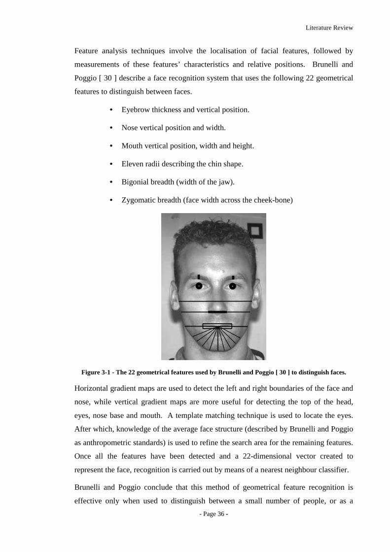
Feature analysis techniques involve the localisation of facial features, followed by
measurements of these features’ characteristics and relative positions. Brunelli and
Poggio [ 30 ] describe a face recognition system that uses the following 22 geometrical
features to distinguish between faces.
• Eyebrow thickness and vertical position.
• Nose vertical position and width.
• Mouth vertical position, width and height.
• Eleven radii describing the chin shape.
• Bigonial breadth (width of the jaw).
• Zygomatic breadth (face width across the cheek-bone)
Figure 3-1 - The 22 geometrical features used by Brunelli and Poggio [ 30 ] to distinguish faces.
Horizontal gradient maps are used to detect the left and right boundaries of the face and
nose, while vertical gradient maps are more useful for detecting the top of the head,
eyes, nose base and mouth. A template matching technique is used to locate the eyes.
After which, knowledge of the average face structure (described by Brunelli and Poggio
as anthropometric standards) is used to refine the search area for the remaining features.
Once all the features have been detected and a 22-dimensional vector created to
represent the face, recognition is carried out by means of a nearest neighbour classifier.
Brunelli and Poggio conclude that this method of geometrical feature recognition is
effective only when used to distinguish between a small number of people, or as a
Literature Review
- Page 3377 --
preliminary screening step, before further classification is performed by another
recognition algorithm. By itself, there does not appear to be enough information within
these 22 geometrical features to classify a large number of people.
Localisation and analysis of these multiple facial features bares some similarity to a
graph matching approaches, which require the construction of a face image graph
representation. Such graphs may encode information based on colour, texture, edge
maps or feature location, but does not necessarily attempt localisation of a specific
facial feature, instead relying on detection of more generic image features such as edge
boundaries, corners and certain texture patterns. The graphs should attempt to collapse
any variance between images of the same person, while emphasising differences
between different people. Recognition is then performed using standard graph-
matching techniques. There are two main difficulties encountered with graph matching
approaches. Firstly, deciding how to generate the nodes of the graph. There are a
limited number of robustly detected features on the face and too few nodes will cause
different graphs to be indistinguishable. Whereas trying to use too many features, some
of which may vary in location size and colour, may cause two graphs of the same face
to have very different structures. Secondly, if the graph is being constructed from a 2D
image of a face, a model may be required to predict the variations in graph structure
caused by varying orientations of the face.
Wiskott et al [ 37 ] present a face recognition method using ‘elastic bunch graphs’. An
attempt is made to recognise faces from a large database containing single images of
people, despite differences in facial expression and head orientation. These variances
are collapsed by extraction of face descriptions in the form of image graphs. The N
nodes of an image graph are made up of a set of fiducial points defined on a face. Some
of which are easily located (e.g. pupils, corners of mouth, tip of nose etc.), while others
are defined as the centre of gravity of these points (e.g. forehead, cheeks, chin etc.).
Each of these nodes is labelled with a jet. A jet being defined as a set of 40 complex
coefficients describing a small patch of grey values around a single pixel, based on a
Gabor wavelet transform. The arcs of image graphs are labelled with two-dimensional
distance vectors, describing the relative locations of the pixels described by the jets at
the graph nodes.
Wiskott et al represents the general face structure in the form of a face bunch graph.
This structure is effectively a collection of image graphs as described above, taken from
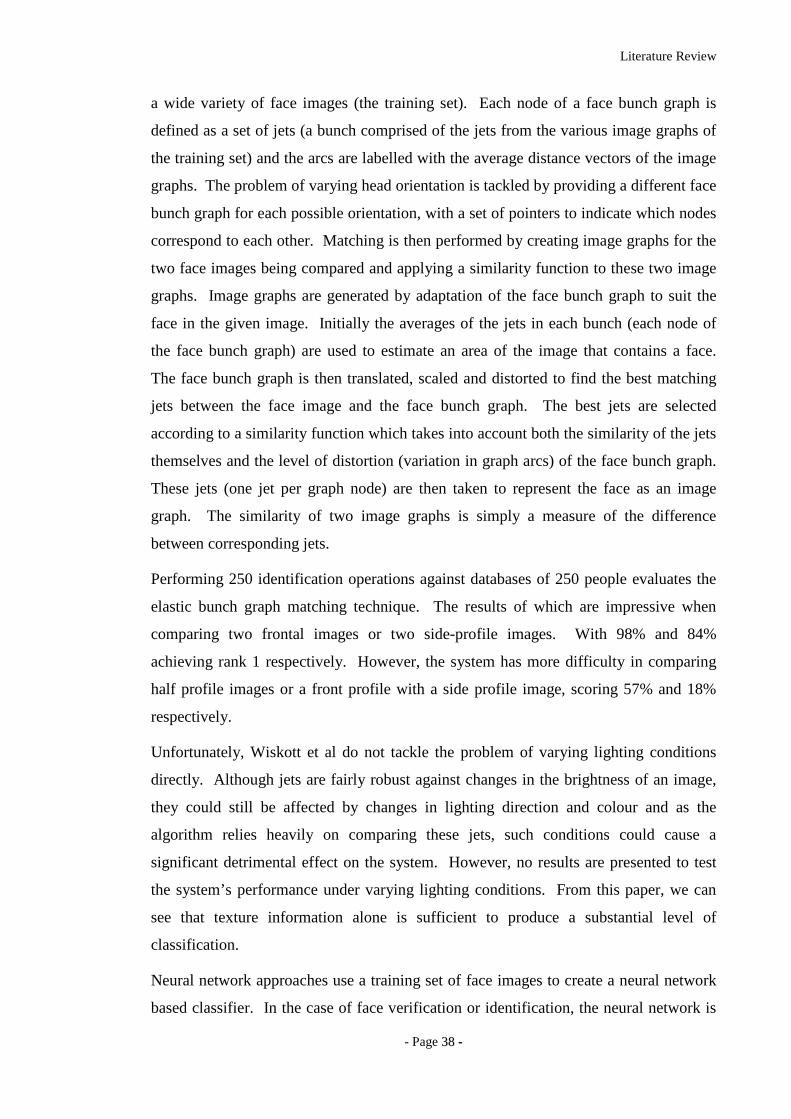
Literature Review
- Page 3388 --
a wide variety of face images (the training set). Each node of a face bunch graph is
defined as a set of jets (a bunch comprised of the jets from the various image graphs of
the training set) and the arcs are labelled with the average distance vectors of the image
graphs. The problem of varying head orientation is tackled by providing a different face
bunch graph for each possible orientation, with a set of pointers to indicate which nodes
correspond to each other. Matching is then performed by creating image graphs for the
two face images being compared and applying a similarity function to these two image
graphs. Image graphs are generated by adaptation of the face bunch graph to suit the
face in the given image. Initially the averages of the jets in each bunch (each node of
the face bunch graph) are used to estimate an area of the image that contains a face.
The face bunch graph is then translated, scaled and distorted to find the best matching
jets between the face image and the face bunch graph. The best jets are selected
according to a similarity function which takes into account both the similarity of the jets
themselves and the level of distortion (variation in graph arcs) of the face bunch graph.
These jets (one jet per graph node) are then taken to represent the face as an image
graph. The similarity of two image graphs is simply a measure of the difference
between corresponding jets.
Performing 250 identification operations against databases of 250 people evaluates the
elastic bunch graph matching technique. The results of which are impressive when
comparing two frontal images or two side-profile images. With 98% and 84%
achieving rank 1 respectively. However, the system has more difficulty in comparing
half profile images or a front profile with a side profile image, scoring 57% and 18%
respectively.
Unfortunately, Wiskott et al do not tackle the problem of varying lighting conditions
directly. Although jets are fairly robust against changes in the brightness of an image,
they could still be affected by changes in lighting direction and colour and as the
algorithm relies heavily on comparing these jets, such conditions could cause a
significant detrimental effect on the system. However, no results are presented to test
the system’s performance under varying lighting conditions. From this paper, we can
see that texture information alone is sufficient to produce a substantial level of
classification.
Neural network approaches use a training set of face images to create a neural network
based classifier. In the case of face verification or identification, the neural network is
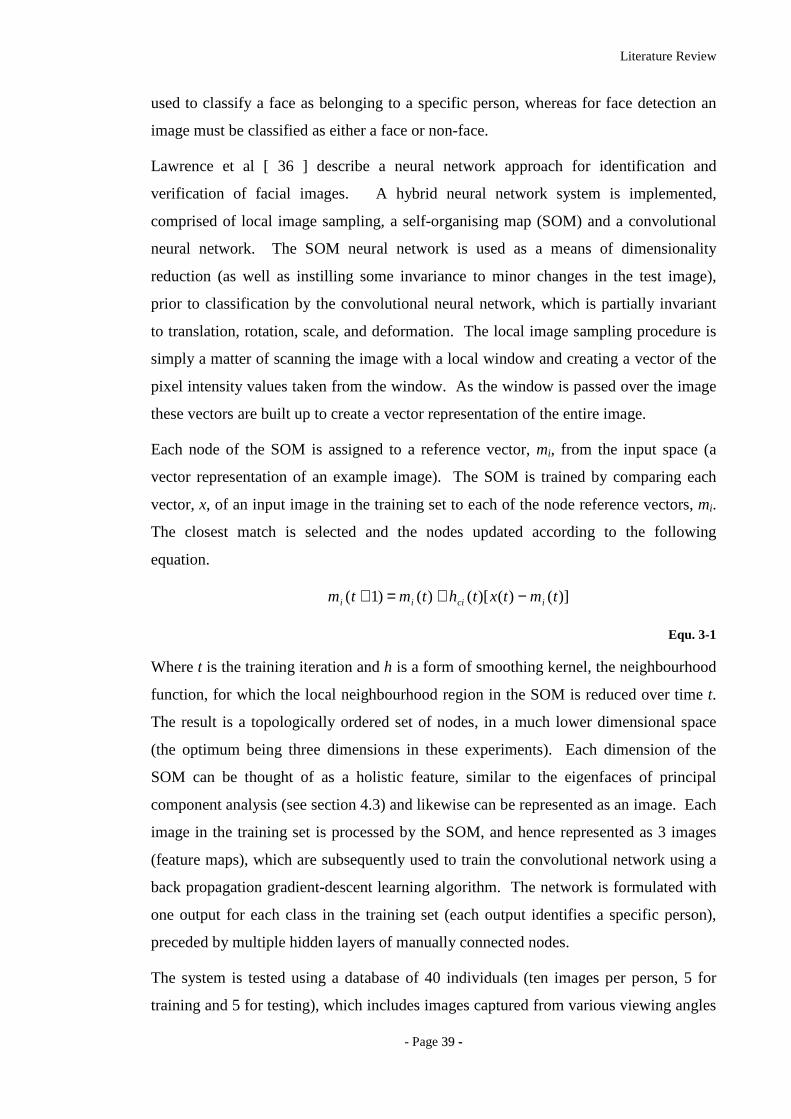
Literature Review
- Page 3399 --
used to classify a face as belonging to a specific person, whereas for face detection an
image must be classified as either a face or non-face.
Lawrence et al [ 36 ] describe a neural network approach for identification and
verification of facial images. A hybrid neural network system is implemented,
comprised of local image sampling, a self-organising map (SOM) and a convolutional
neural network. The SOM neural network is used as a means of dimensionality
reduction (as well as instilling some invariance to minor changes in the test image),
prior to classification by the convolutional neural network, which is partially invariant
to translation, rotation, scale, and deformation. The local image sampling procedure is
simply a matter of scanning the image with a local window and creating a vector of the
pixel intensity values taken from the window. As the window is passed over the image
these vectors are built up to create a vector representation of the entire image.
Each node of the SOM is assigned to a reference vector, mi, from the input space (a
vector representation of an example image). The SOM is trained by comparing each
vector, x, of an input image in the training set to each of the node reference vectors, mi.
The closest match is selected and the nodes updated according to the following
equation.
)]()()[()()1( tmtxthtmtm iciii −+=+
Equ. 3-1
Where t is the training iteration and h is a form of smoothing kernel, the neighbourhood
function, for which the local neighbourhood region in the SOM is reduced over time t.
The result is a topologically ordered set of nodes, in a much lower dimensional space
(the optimum being three dimensions in these experiments). Each dimension of the
SOM can be thought of as a holistic feature, similar to the eigenfaces of principal
component analysis (see section 4.3) and likewise can be represented as an image. Each
image in the training set is processed by the SOM, and hence represented as 3 images
(feature maps), which are subsequently used to train the convolutional network using a
back propagation gradient-descent learning algorithm. The network is formulated with
one output for each class in the training set (each output identifies a specific person),
preceded by multiple hidden layers of manually connected nodes.
The system is tested using a database of 40 individuals (ten images per person, 5 for
training and 5 for testing), which includes images captured from various viewing angles
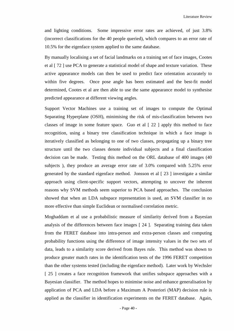
Literature Review
- Page 4400 --
and lighting conditions. Some impressive error rates are achieved, of just 3.8%
(incorrect classifications for the 40 people queried), which compares to an error rate of
10.5% for the eigenface system applied to the same database.
By manually localising a set of facial landmarks on a training set of face images, Cootes
et al [ 72 ] use PCA to generate a statistical model of shape and texture variation. These
active appearance models can then be used to predict face orientation accurately to
within five degrees. Once pose angle has been estimated and the best-fit model
determined, Cootes et al are then able to use the same appearance model to synthesise
predicted appearance at different viewing angles.
Support Vector Machines use a training set of images to compute the Optimal
Separating Hyperplane (OSH), minimising the risk of mis-classification between two
classes of image in some feature space. Guo et al [ 22 ] apply this method to face
recognition, using a binary tree classification technique in which a face image is
iteratively classified as belonging to one of two classes, propagating up a binary tree
structure until the two classes denote individual subjects and a final classification
decision can be made. Testing this method on the ORL database of 400 images (40
subjects ), they produce an average error rate of 3.0% compared with 5.25% error
generated by the standard eigenface method. Jonsson et al [ 23 ] investigate a similar
approach using client-specific support vectors, attempting to uncover the inherent
reasons why SVM methods seem superior to PCA based approaches. The conclusion
showed that when an LDA subspace representation is used, an SVM classifier in no
more effective than simple Euclidean or normalised correlation metric.
Moghaddam et al use a probabilistic measure of similarity derived from a Bayesian
analysis of the differences between face images [ 24 ]. Separating training data taken
from the FERET database into intra-person and extra-person classes and computing
probability functions using the difference of image intensity values in the two sets of
data, leads to a similarity score derived from Bayes rule. This method was shown to
produce greater match rates in the identification tests of the 1996 FERET competition
than the other systems tested (including the eigenface method). Later work by Wechsler
[ 25 ] creates a face recognition framework that unifies subspace approaches with a
Bayesian classifier. The method hopes to minimise noise and enhance generalisation by
application of PCA and LDA before a Maximum A Posteriori (MAP) decision rule is
applied as the classifier in identification experiments on the FERET database. Again,
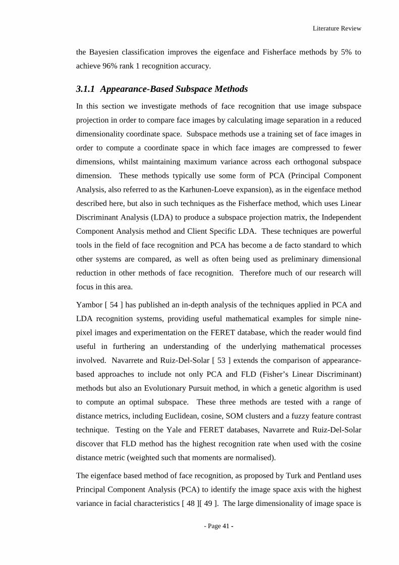
Literature Review
- Page 4411 --
the Bayesien classification improves the eigenface and Fisherface methods by 5% to
achieve 96% rank 1 recognition accuracy.
3.1.1 Appearance-Based Subspace Methods
In this section we investigate methods of face recognition that use image subspace
projection in order to compare face images by calculating image separation in a reduced
dimensionality coordinate space. Subspace methods use a training set of face images in
order to compute a coordinate space in which face images are compressed to fewer
dimensions, whilst maintaining maximum variance across each orthogonal subspace
dimension. These methods typically use some form of PCA (Principal Component
Analysis, also referred to as the Karhunen-Loeve expansion), as in the eigenface method
described here, but also in such techniques as the Fisherface method, which uses Linear
Discriminant Analysis (LDA) to produce a subspace projection matrix, the Independent
Component Analysis method and Client Specific LDA. These techniques are powerful
tools in the field of face recognition and PCA has become a de facto standard to which
other systems are compared, as well as often being used as preliminary dimensional
reduction in other methods of face recognition. Therefore much of our research will
focus in this area.
Yambor [ 54 ] has published an in-depth analysis of the techniques applied in PCA and
LDA recognition systems, providing useful mathematical examples for simple nine-
pixel images and experimentation on the FERET database, which the reader would find
useful in furthering an understanding of the underlying mathematical processes
involved. Navarrete and Ruiz-Del-Solar [ 53 ] extends the comparison of appearance-
based approaches to include not only PCA and FLD (Fisher’s Linear Discriminant)
methods but also an Evolutionary Pursuit method, in which a genetic algorithm is used
to compute an optimal subspace. These three methods are tested with a range of
distance metrics, including Euclidean, cosine, SOM clusters and a fuzzy feature contrast
technique. Testing on the Yale and FERET databases, Navarrete and Ruiz-Del-Solar
discover that FLD method has the highest recognition rate when used with the cosine
distance metric (weighted such that moments are normalised).
The eigenface based method of face recognition, as proposed by Turk and Pentland uses
Principal Component Analysis (PCA) to identify the image space axis with the highest
variance in facial characteristics [ 48 ][ 49 ]. The large dimensionality of image space is
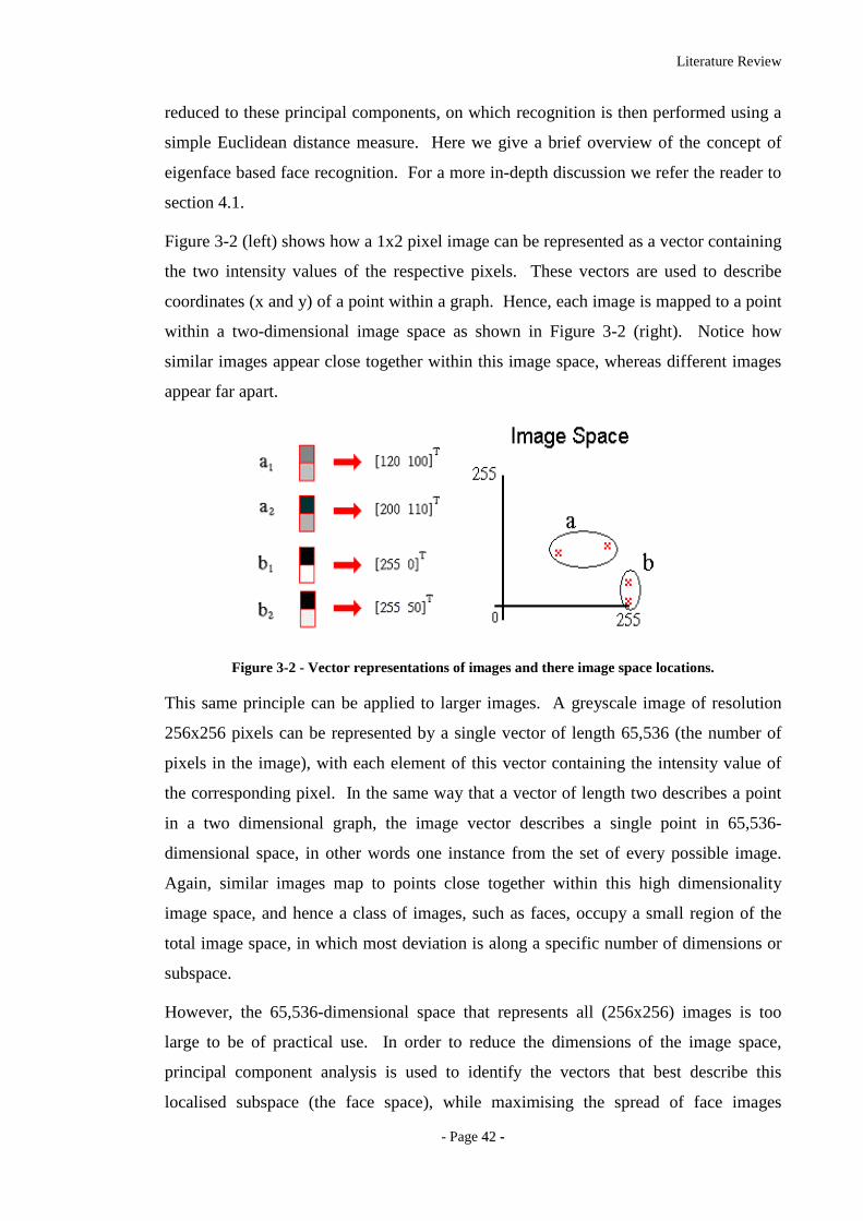
Literature Review
- Page 4422 --
reduced to these principal components, on which recognition is then performed using a
simple Euclidean distance measure. Here we give a brief overview of the concept of
eigenface based face recognition. For a more in-depth discussion we refer the reader to
section 4.1.
Figure 3-2 (left) shows how a 1x2 pixel image can be represented as a vector containing
the two intensity values of the respective pixels. These vectors are used to describe
coordinates (x and y) of a point within a graph. Hence, each image is mapped to a point
within a two-dimensional image space as shown in Figure 3-2 (right). Notice how
similar images appear close together within this image space, whereas different images
appear far apart.
Figure 3-2 - Vector representations of images and there image space locations.
This same principle can be applied to larger images. A greyscale image of resolution
256x256 pixels can be represented by a single vector of length 65,536 (the number of
pixels in the image), with each element of this vector containing the intensity value of
the corresponding pixel. In the same way that a vector of length two describes a point
in a two dimensional graph, the image vector describes a single point in 65,536-
dimensional space, in other words one instance from the set of every possible image.
Again, similar images map to points close together within this high dimensionality
image space, and hence a class of images, such as faces, occupy a small region of the
total image space, in which most deviation is along a specific number of dimensions or
subspace.
However, the 65,536-dimensional space that represents all (256x256) images is too
large to be of practical use. In order to reduce the dimensions of the image space,
principal component analysis is used to identify the vectors that best describe this
localised subspace (the face space), while maximising the spread of face images
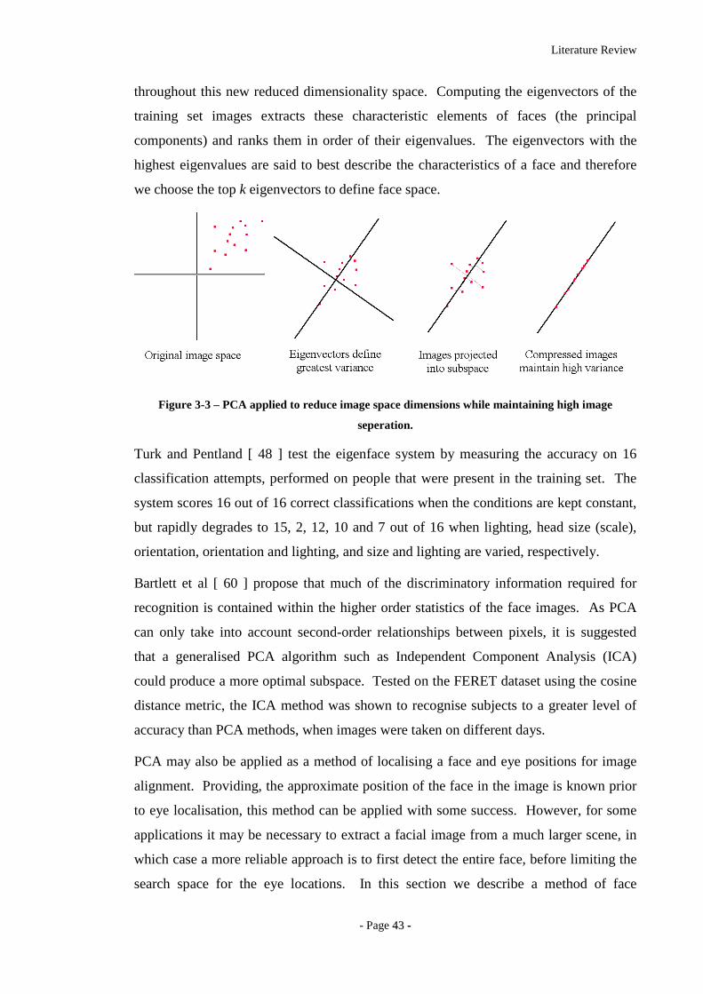
Literature Review
- Page 4433 --
throughout this new reduced dimensionality space. Computing the eigenvectors of the
training set images extracts these characteristic elements of faces (the principal
components) and ranks them in order of their eigenvalues. The eigenvectors with the
highest eigenvalues are said to best describe the characteristics of a face and therefore
we choose the top k eigenvectors to define face space.
Figure 3-3 – PCA applied to reduce image space dimensions while maintaining high image
seperation.
Turk and Pentland [ 48 ] test the eigenface system by measuring the accuracy on 16
classification attempts, performed on people that were present in the training set. The
system scores 16 out of 16 correct classifications when the conditions are kept constant,
but rapidly degrades to 15, 2, 12, 10 and 7 out of 16 when lighting, head size (scale),
orientation, orientation and lighting, and size and lighting are varied, respectively.
Bartlett et al [ 60 ] propose that much of the discriminatory information required for
recognition is contained within the higher order statistics of the face images. As PCA
can only take into account second-order relationships between pixels, it is suggested
that a generalised PCA algorithm such as Independent Component Analysis (ICA)
could produce a more optimal subspace. Tested on the FERET dataset using the cosine
distance metric, the ICA method was shown to recognise subjects to a greater level of
accuracy than PCA methods, when images were taken on different days.
PCA may also be applied as a method of localising a face and eye positions for image
alignment. Providing, the approximate position of the face in the image is known prior
to eye localisation, this method can be applied with some success. However, for some
applications it may be necessary to extract a facial image from a much larger scene, in
which case a more reliable approach is to first detect the entire face, before limiting the
search space for the eye locations. In this section we describe a method of face
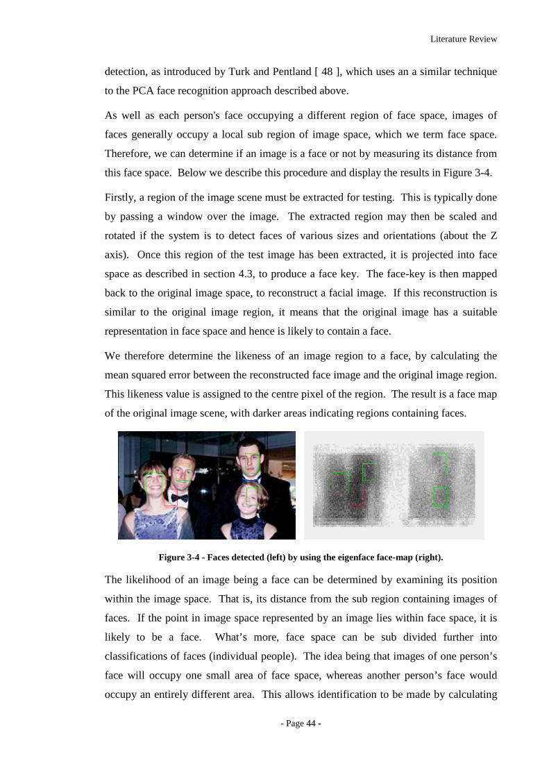
Literature Review
- Page 4444 --
detection, as introduced by Turk and Pentland [ 48 ], which uses an a similar technique
to the PCA face recognition approach described above.
As well as each person's face occupying a different region of face space, images of
faces generally occupy a local sub region of image space, which we term face space.
Therefore, we can determine if an image is a face or not by measuring its distance from
this face space. Below we describe this procedure and display the results in Figure 3-4.
Firstly, a region of the image scene must be extracted for testing. This is typically done
by passing a window over the image. The extracted region may then be scaled and
rotated if the system is to detect faces of various sizes and orientations (about the Z
axis). Once this region of the test image has been extracted, it is projected into face
space as described in section 4.3, to produce a face key. The face-key is then mapped
back to the original image space, to reconstruct a facial image. If this reconstruction is
similar to the original image region, it means that the original image has a suitable
representation in face space and hence is likely to contain a face.
We therefore determine the likeness of an image region to a face, by calculating the
mean squared error between the reconstructed face image and the original image region.
This likeness value is assigned to the centre pixel of the region. The result is a face map
of the original image scene, with darker areas indicating regions containing faces.
Figure 3-4 - Faces detected (left) by using the eigenface face-map (right).
The likelihood of an image being a face can be determined by examining its position
within the image space. That is, its distance from the sub region containing images of
faces. If the point in image space represented by an image lies within face space, it is
likely to be a face. What’s more, face space can be sub divided further into
classifications of faces (individual people). The idea being that images of one person’s
face will occupy one small area of face space, whereas another person’s face would
occupy an entirely different area. This allows identification to be made by calculating

Literature Review
- Page 4455 --
the distance between image locations in face space with a known person’s location in
face space.
The Fisherface based method of face recognition as described by Belhumeur et al [ 27
], uses both PCA and LDA to produce a linear projection into a low dimensional
subspace, similar to that used in the eigenface method. However, the Fisherface method
is able to take advantage of ‘within-class’ information to maximise class separation.
This means that the training set for the Fisherface method can utilise multiple images of
each person to determine within-class variation (whereas eigenface typically uses only
one image per person), allowing any variation between images of the same person to be
minimised in the classification process. This is the Fisherface method’s main advantage
over the eigenface method. We are able to specify (by providing examples in the
training set) how a person’s face may change from one image to another, due to
variations in lighting conditions facial expression and even small changes in orientation.
The idea being, that by providing a set of images of each person taken under various
lighting conditions and facial expressions, this method becomes more immune to such
changes.
Belhumeur et al [ 27 ] point out that the eigenface method maximises the total scatter
across all faces within face space, thus retaining some of the unwanted variations
(caused by lighting and facial expression). For example, if one of the faces within the
training set had an open mouth, this 'feature' would contribute to the scatter of the face
images within face space, meaning that an open mouth is identified as a discriminating
characteristic between people. Anyone with an open mouth would therefore begin to
look similar (within face space). Whereas the Fisherface method could use multiple
images of a person with an open and closed mouth to enforce the fact that the
appearance of a mouth can change from one image to another, in which case it will have
little influence in the classification process.
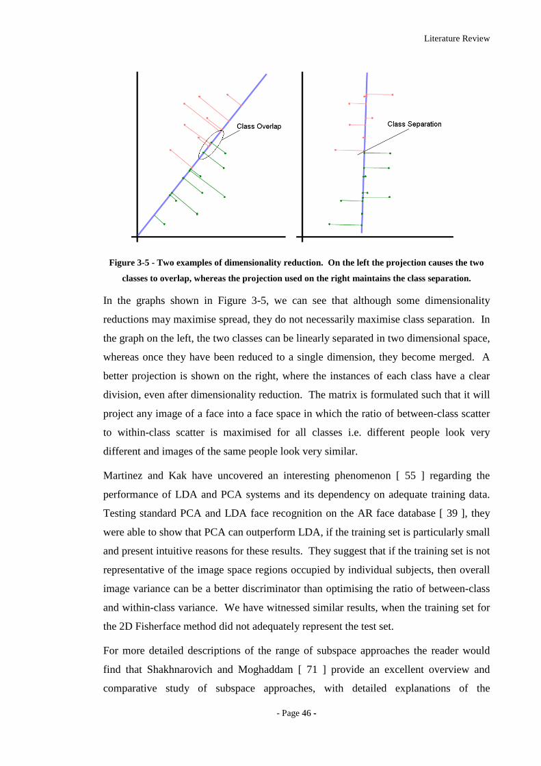
Literature Review
- Page 4466 --
Figure 3-5 - Two examples of dimensionality reduction. On the left the projection causes the two
classes to overlap, whereas the projection used on the right maintains the class separation.
In the graphs shown in Figure 3-5, we can see that although some dimensionality
reductions may maximise spread, they do not necessarily maximise class separation. In
the graph on the left, the two classes can be linearly separated in two dimensional space,
whereas once they have been reduced to a single dimension, they become merged. A
better projection is shown on the right, where the instances of each class have a clear
division, even after dimensionality reduction. The matrix is formulated such that it will
project any image of a face into a face space in which the ratio of between-class scatter
to within-class scatter is maximised for all classes i.e. different people look very
different and images of the same people look very similar.
Martinez and Kak have uncovered an interesting phenomenon [ 55 ] regarding the
performance of LDA and PCA systems and its dependency on adequate training data.
Testing standard PCA and LDA face recognition on the AR face database [ 39 ], they
were able to show that PCA can outperform LDA, if the training set is particularly small
and present intuitive reasons for these results. They suggest that if the training set is not
representative of the image space regions occupied by individual subjects, then overall
image variance can be a better discriminator than optimising the ratio of between-class
and within-class variance. We have witnessed similar results, when the training set for
the 2D Fisherface method did not adequately represent the test set.
For more detailed descriptions of the range of subspace approaches the reader would
find that Shakhnarovich and Moghaddam [ 71 ] provide an excellent overview and
comparative study of subspace approaches, with detailed explanations of the

Literature Review
- Page 4477 --
mathematical techniques involved in PCA, LDA and ICA methods as well as Bayesian
approaches and modular face recognition algorithms. For performance evaluations, a
comparison of results produced by many face recognition systems on a common
database is provided in the documentation of the Face Recognition Vendor Tests [ 1 ].
Although including systems implemented by commercial organisations (and therefore
not disclosing exact details of the method used), the FRVT does give a good indication
of the current error rates of state-of-the-art systems and provides a benchmark by which
to gauge the potential of any new method.
Literature Review
- Page 4488 --
33..22 33DD AApppprr ooaacchheess
Although limited when compared with the wealth of research applied to 2D face
recognition, there are a number of investigations that demonstrate how geometric facial
structure can be used to aid recognition. Zhao and Chellappa [ 9 ] use a generic 3D face
model to normalise facial orientation and lighting direction prior to recognition,
increasing accuracy from approximately 81% (correct match within rank of 25) to 100%
when applied to the Weizmann database. A generic 3D face model is scaled and
aligned to match a 2D target image. If the head is not orientated appropriately (frontal
profile), Zhao and Chellappa use the generic 3D face model, together with light source
direction and pose estimations, to compensate by producing a prototype image of the
frontal pose equivalent. Face recognition is then performed on this prototype image.
Similar improvements are witnessed in the Face Recognition Vendor Test [ 1 ], showing
that pose correction using Romdhani et al’s 3D morphable model technique [ 10 ]
reduces error rates when applied to the FERET database. This method is analysed and
discussed in more detail by Blanz et al [ 11 ], using a 3D morphable face model to aid in
identification of 2D face images. Beginning with an initial estimate of lighting
direction and face shape, Blanz et al iteratively alters shape and texture parameters of
the morphable face model, minimising difference to the two-dimensional image. These
parameters are then taken as features for identification, resulting in 82.6% correct
identifications on a test set of 68 people.
This same technique of generating 3D morphable models from 2D images has been
utilised in other experiments, such as Huang et al’s component based face recognition
approach using 3D morphable models to improve recognition accuracy when pose and
illumination are unknown [ 56 ]. Taking a Support Vector Machine (SVM) approach
developed in previous work [ 58 ], in which a face image is decomposed into smaller
components interconnected by a flexible geometric model, Huang et al tackle the
problem of a large training set requisite by synthesising many 2D training images from
3D face models under varying pose and virtual lighting conditions. The 3D morphable
model is initially generated from three 2D images as described in Blanz and Vetter’s
earlier research [ 57 ], before numerous face images are synthesised. These images are
then separated into components and used to train a second-degree polynomial SVM
Literature Review
- Page 4499 --
classifier. Recognition accuracy is reported at 90%, compared with a comparable global
face recognition method achieving 40%.
Bronstein et al [ 59 ] uses photometric stereo techniques to compute facial surface shape
from numerous 2D images, acquired under varying lighting conditions. Surface
gradient is used by a Fast Marching on Triangulated Domains (FMTD) algorithm to
produce a map of geodesic distances across the facial surface without the need to
reconstruct an actual 3D face model. Moments of a cononical form of this geodesic
map are extracted as a face signature and compared using the Euclidean distance metric.
Taking images of seven subjects from the Yale Face Database, Bronstein et al were able
to show that within-class and between-class standard deviations were improved by an
order of magnitude, compared with the direct comparison of facial surface gradients.
Although these methods show that knowledge of 3D face shape can aid normalisation
for two-dimensional face recognition systems, none of the methods mentioned so far
use actual geometric structure to perform recognition. However, the research does
demonstrate that 3D facial information can be used extremely effectively to eliminate
some of the problems encountered with 2D recognition (i.e. pose and illumination),
even when only a generic 3D model is used. It is likely that if the actual geometric
shape information of a subjects face contributed to the recognition process further
improvements could be made.
To test the use of geometric shape data for recognition a preliminary investigation was
carried out at the University of York by Turner and Austin [ 46 ] exploring the
possibilities of using AURA (Advanced Uncertain Reasoning Architecture) [ 46 ][ 47 ]
technology in conjunction with a graph-matching algorithm to perform face recognition.
AURA is an architecture based on a pattern-matching concept utilising correlation
matrix memories, with the key advantage of an extremely efficient hardware
implementation, in the form of the Presence PCI card (or more recently the Presence II
card) [ 62 ]. These devices are able to search onboard memory extremely quickly for
matching patterns. What’s more, because these devices are able to operate in parallel, a
large database of face models may be distributed between several Presence II cards.
The matching algorithm used the Relaxation By Elimination (RBE) graph matching
techniques. This algorithm has several properties that make it particularly suitable for
face recognition. Firstly, the neural network architecture (Correlation Matrix
Memories) of the AURA system means that even noisy or incomplete data (e.g. caused

Literature Review
- Page 5500 --
by wearing glasses, non-frontal head orientation or bright specula reflection) can still
result in a successful match. Anomalies are effectively ignored and performance
degrades gracefully in the presence of increasing noise and occlusion.
Although limited in terms of test data, the investigation demonstrated that the AURA
graph matcher is capable of distinguishing between facial surfaces based on 3D
geometry alone. However, the research was not pursued much further, as error rates
remained relatively high compared to the more promising avenues of the eigensurface
and Fishersurface methods (see sections 5.5 and 5.6). Despite this, because AURA
architecture is able to operate independently of the CPU, it could be used to search a
database of face models, pruning the most unlikely matches from the search space as an
initial screening step. A large database could then be reduced to a small set of possible
matches before a more rigorous algorithm is applied. Hence, allowing matching
techniques that may not scale well to be applied to large databases. We supply the
results of this investigation in Appendix II.
Beumier and Acheroy also make use of 3D surface information, by performing face
recognition using a surface matching approach on the 3D facial structure [ 5 ][ 3 ].
These 3D facial surfaces are generated from a single image taken of a person’s face,
onto which structured light (stripes) are projected. The 3D structure of the face is
computed by measuring the deformation of the stripes across the face. Some orientation
normalisation is then required to ensure a consistent fronto-parallel view. This
normalisation is performed by generating some initial parameters for the three angles of
rotation and three directions of translation (based on nose detection, forehead and cheek
angle), before refining the search until the minimum distance is found between the two
facial surfaces being compared.
The paper describes various methods of matching the 3D facial surfaces. However, few
methods were successful due to the nature of the 3D data obtained (which often
contained high levels of noise). Curvature analysis proved ineffective, (again due to the
noise present in the 3D surface). Feature extraction also proved difficult, probably due
to the lack of detail in the model, resulting in the nose being the only reliably located
feature. Despite this, they still managed to produce some good results using two
methods of surface matching by means of comparing profiles extracted from the 3D
facial surface. The first method extracts 15 profiles, by taking the intersection of the
facial surface with evenly spaced vertical planes. These profile curves are compared by

Literature Review
- Page 5511 --
dividing the area between the curves by the arc length, giving a distance measure.
Beumier and Acheroy carry out verification tests on a database of 30 people, giving an
EER between 9% and 13% when using automatic alignment, but dropping to between
3.25% and 6% if manual alignment is used.
The second method is to take one central profile and two lateral profiles, which are
converted into one-dimensional vectors of local curvature values. The left and right
lateral profiles are averaged to give a mean lateral profile. Facial surfaces are then
compared by calculating the difference between these curvature values of the central
and mean lateral profile. This method gives improved EERs of between 7.25% and 9%
on the automatically aligned surfaces and between 6.25% and 9.5% on the manually
aligned surfaces.
Although the database used is too small to make any firm conclusions, Beumier and
Acheroy’s research does suggest that:
• There is enough information to achieve a high level of face recognition
accuracy in the facial 3D geometrical structure alone.
• A high level of accuracy (low levels of noise, missing data, spikes etc.)
and precision (depth resolution) of the 3D data is essential for good
performance.
• Few features can be reliably localised based on the geometrical structure
alone. Therefore, a system that relies heavily on locating many features
and measuring distances between them is likely to produce poor results.
• The performance of the orientation normalisation procedure has a
significant influence on the overall system performance.
Another approach is taken by Chua et al [ 8 ], using point signature as a non-rigid object
representation, on which recognition can then be performed. Chua et al treats the face
recognition problem as a 3D recognition problem of non-rigid surfaces. By observing
range data of various facial expressions, it is noted that certain areas of the face remain
rigid while other areas are able to deform significantly. An attempt is made to extract
these rigid areas of the face for recognition, thus creating a system that is invariant to
facial expression. It is also hoped that by ignoring large areas of the face that are

Literature Review
- Page 5522 --
unstable, the size of the models used for comparison will be greatly reduced, leading to
a decrease in recognition time and space complexity.
The characteristic used to identify these rigid areas of faces and ultimately to distinguish
between faces is the point signature, which describes the depth values surrounding the
local region of a specific point on the facial surface. The point signature for any point p
on a facial surface, is defined as a discrete set of values d(
i) where 0 <
i < 360 and
= 10. Each value d(
i) is the distance from a point at angle
i on a 3D curve C (defined
as the intersection of a sphere of radius r, centred at point p, with the facial surface) to
the corresponding point on the perpendicular projection of the 3D curve C`. The
comparison of two point signatures ds(
i) and dm(
i) is performed using the following
equation.
θθεθθ nidd itolimis ,...,1)()()( =∀<−
Equ. 3-2
Where tol(
i) is a set of tolerance values configured to produce the best acceptance and
rejection rates. For a more in-depth discussion of point signature generation and
comparison, we refer the reader to Chua et al's paper [ 8 ]. The first stage of point
signature based recognition is the registration of 3D faces: performed by finding 3
points on each of two facial surfaces for which the following constraints hold:
• The point signatures of corresponding points match.
• The distances between the 3 points on one face, and the 3 points on the
other face are within an error tolerance (possibly under various scales).
Once the three corresponding points on each face have been found the two facial
surfaces can be aligned. Distances between the two facial surfaces are then measured
according to a Gaussian distribution model and areas with a low distance measure are
extracted as rigid areas. Two facial surfaces are compared by extracting the rigid areas
of the face then generating point signatures for all points on the remaining facial
surface. This set is reduced to a set of unique point signatures, which are then compared
to the corresponding point signatures on the other facial surface.
Chua et al gather results from a set of range images taken from 6 different people. A
total of 30 range images are used (four different expressions for each person, plus one
probe image). The probe image is identified correctly for all six people. However, the
Literature Review
- Page 5533 --
separation of scores is not particularly large. With the correct scores ranging from
93.75 % to 78.85% and the highest incorrect score being 76.92%.
Coombes et al [ 32 ] present a method of mathematically describing facial surface
shape, based on differential geometry. Curvature analysis is performed on a depth map
of the facial surface, to produce segmentation into one of eight fundamental surface
types. Coombes et al stress the need for the depth map of a facial surface to be created
from a specific viewpoint, therefore giving the prerequisite of some 3D facial
alignment. They also describes several methods of computing the curvature of the
facial surface and describe the advantages of a method developed by Coombes and
Richards, which takes into account the possible error due to lack of detail when surfaces
are at a sharp angle to the viewpoint.
The facial surface can be segmented into the eight surface types, based on the sign of
the curvature: peak, ridge, saddle ridge, minimal, pit, valley, saddle valley and flat.
Coombes et al suggest that two faces may be distinguished by comparing which regions
of the two faces are classified as the various surface types. Prior to two facial surfaces
being compared, they must first be registered. This is done by manually selecting
several corresponding feature locations on each face, which are then used to scale,
translate and rotate, such that two facial surfaces are aligned. Using this method, 3D
facial surfaces have been produced for the average female and average male face,
showing distinct differences in chin structure, nose shape, forehead shape and cheek
bone position. A quantitative analysis of the average male and average female facial
surfaces shows that the main differences are of prominence or retrusion in specific areas
of the face.
Hesher et al [ 6 ] use PCA of depth maps and a Euclidean distance metric to perform
identification with 94% accuracy on 37 face models (when training is performed on the
gallery set). Our own investigations of a similar method are presented in section 5.5
(also published by Heseltine et al [ 16 ]), showing how different surface representations
and distance measures affect recognition, reducing the EER from 19.1% to 12.7% when
applied to a test set of 290 face models acquired under difficult capture conditions such
as variations in head angle and expressions.
Gordon [ 4 ] takes a feature based approach, based on both depth and curvature
information. It is stated that curvature data is easily derived from the range data, and

Literature Review
- Page 5544 --
has substantial advantages. It has the potential for higher accuracy in describing surface
based events and it is better suited to describing properties around facial regions such as
the cheeks, forehead and chin. It is also viewpoint invariant. Gordon uses facial feature
localisation and absolute measurements (millimetres rather than pixels) to calculate a set
of feature descriptors from the 3D data.
The usefulness of a feature for the purpose of classification is dependent on its ability to
discriminate between people. To evaluate the set of features, a value is calculated
indicating the level of discrimination for each feature, this property is Fishers linear
discriminant (FLD), as shown in the equation below.
∑ ∑
∑
= Φ∈
=
−
−=
c
i xin
c
ii
i
imx
mmd
1
21
1
2
)(
)(
Equ. 3-3
Where d describes the discriminating power of a feature , between c different classes
(people). i is the set (size ni) of feature values of class i, and mi and m are the means
of i and feature values of all classes respectively. The features tested by Gordon are
shown in Table 3-1.
Gordon continues to create a face recognition system by means of a simple Euclidean
distance measure in feature space. Several combinations of features are tested using a
database of 24 facial surfaces (8 different people), defining a correct recognition if the
subject was selected as the top match from the database (lowest distance measure).
Results range from 70.8% to 100% correct recognition, with the best score achieved by
using the first 6 features of Table 3-1. A linear degradation was observed when using
greater or fewer features.
Bronstein et al have investigated the use of texture mapped 3D face models focusing on
expression invariant face recognition [ 61 ] using geometric invariants of the face
extracted from 3D face data for non-rigid surface comparisons. By using isometric
surface signatures known as bending-invariant cononical forms, generated by
dimensionality reduction through multidimensional scaling, Bronstein et al compare
signatures by a weighted Euclidean distance metric. Testing the method on a database
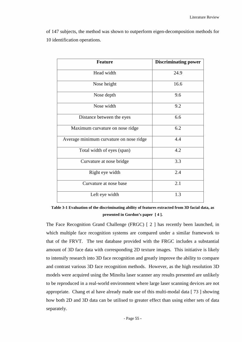
Literature Review
- Page 5555 --
of 147 subjects, the method was shown to outperform eigen-decomposition methods for
10 identification operations.
Feature Discriminating power
Head width 24.9
Nose height 16.6
Nose depth 9.6
Nose width 9.2
Distance between the eyes 6.6
Maximum curvature on nose ridge 6.2
Average minimum curvature on nose ridge 4.4
Total width of eyes (span) 4.2
Curvature at nose bridge 3.3
Right eye width 2.4
Curvature at nose base 2.1
Left eye width 1.3
Table 3-1 Evaluation of the discriminating ability of features extracted from 3D facial data, as
presented in Gordon’s paper [ 4 ].
The Face Recognition Grand Challenge (FRGC) [ 2 ] has recently been launched, in
which multiple face recognition systems are compared under a similar framework to
that of the FRVT. The test database provided with the FRGC includes a substantial
amount of 3D face data with corresponding 2D texture images. This initiative is likely
to intensify research into 3D face recognition and greatly improve the ability to compare
and contrast various 3D face recognition methods. However, as the high resolution 3D
models were acquired using the Minolta laser scanner any results presented are unlikely
to be reproduced in a real-world environment where large laser scanning devices are not
appropriate. Chang et al have already made use of this multi-modal data [ 73 ] showing
how both 2D and 3D data can be utilised to greater effect than using either sets of data
separately.
Literature Review
- Page 5566 --
33..33 RReeccooggnnii tt iioonn DDii ff ff iiccuull tt iieess
The problems caused by changes in lighting conditions have been well researched.
Adini, Moses and Ullman suggest that the difference (mean square intensity difference
on a pixel basis) between images of one face under different illumination conditions are
greater than the differences between images of different faces under the same
illumination conditions [ 26 ]. It has been attempted, with some success, to identify and
compensate for the effect of lighting conditions in various face recognition systems.
Zhao and Chellappa use a generic 3D surface of a face, together with a varying albedo
reflectance model and a Lambertian physical reflectance model to compensate for both
the lighting and head orientation [ 9 ], before applying a recognition system based on
LDA.
Much research has also been carried out to improve eigenface recognition systems.
Cutler has shown that it can successfully be applied to infrared images [ 7 ], resulting in
a much decreased error rate. This shows that an artificial infrared light source could be
used to reduce the effect of external light sources, producing an accurate system for use
in security applications such as site access. However, the use of such a light source is
not always practical, particularly if the camera is far from the subject.
Pentland, Moghaddam and Starner extended their eigenface system to include multiple
viewing angles of a person’s face [ 40 ], improving the system performance when
applied to faces of various orientations. This was done by gathering several training
sets, each containing images of people's faces from a specific angle. When recognition
is performed, the face image is projected into the appropriate face space (depending on
the orientation of the face in the image determined according to the distance from face
space). Although this method does expand the systems capabilities, as the angle of
orientation deviates from the fronto-parallel view, the system’s performance degrades.
Pentland et al also incorporate a modular eigenface system [ 40 ], which significantly
improves the overall performance, although it does not tackle the lighting problem
directly. Belhumeur, Hespanha and Kreigman use Fisher’s linear discriminant to
capture similarities between multiple images in each class (per person) [ 27 ], hoping to
discount variations due to lighting from the defined subspace. Their results show a
significant improvement over the standard eigenface approach (from 20% to less than
Literature Review
- Page 5577 --
2% error rate). However, it does not overcome the problem of changes in lighting
conditions.
33..44 HHuummaann FFaacciiaall PPeerr cceepptt iioonn
In this section we take a slight deviation from the computer science perspective and
review some literature that focuses on the ability of the human visual system to perform
face recognition. Whether or not this line of investigation will prove useful in the quest
to design an improved automatic face recognition technique remains to be seen,
however we must remember that one of the main driving forces behind automated face
recognition research is that we (humans) recognise people by a similar means.
Automatic face recognition systems will always have this analogy to human perception,
meaning a systems decision can easily be verified by a human operator. In addition,
this concept provides some comfort in that we are not trying to tackle an impossible
problem, a system has already been created that can perform this task: the human brain.
However, we must be cautious regarding this statement. We are all aware of our
impressive ability to recognise a close friend in a blurred image, partially occluded with
dark glasses, at a glance across a crowded room, even if we have not seen them for
several years (something that is far beyond the capability of any existing face
recognition system). On the other hand, our face recognition ability can be surprisingly
poor, given just a single photograph of somebody we have never met we often fail to
recognise another image if a small change in lighting has occurred, conversely we can
easily misidentify somebody because of a similar moustache, hairstyle or other features.
If we relate this to our expectation of an automated face recognition system (instant
recognition from a single reference image when compared against thousands of images
in unknown conditions), perhaps automated systems have already surpassed human
recognition. If so, this is a persuasive argument for adoption of a face recognition
system in any scenario where identification is currently carried out by a human operator.
For these reasons, this topic is worthy of some attention, in particular with regard to the
following questions:
• How do humans recognise faces?
• Is there any correlation between human perception and automatic
methods of recognition?

Literature Review
- Page 5588 --
• Is there any value in attempting to emulate methods of human face
recognition in order to improve existing systems?
• How good is human face recognition and at what point does an
automated method become more effective than a human operator?
Burton et al [ 70 ] shows that familiarity of faces is very important for human facial
recognition, especially when image quality is poor. By testing the ability of humans to
recognise faces in poor quality security videos it was shown that if a person is familiar
with a subject they can be recognised to a high degree of success (even in very poor
conditions), compared to people who were unfamiliar with the subject (including police
officers experienced in forensic identification). By performing two experiments, either
obscuring the body of the subject (to eliminate cues from gait and clothing) or just the
face region, Burton et al demonstrates that the face is by far the primary cue for
recognition.
Another paper by Burton et al [ 69 ] has shown that a cognitive model of face
recognition in combination with PCA can be used to simulate computation of
familiarity, perhaps suggesting some commonality between the holistic appearance-
based PCA methods of face recognition and the feature extraction of human facial
perception. Hancock, Bruce and Burton [ 12 ][ 13 ] extend this comparison, contrasting
the capabilities of the human visual system to that of PCA methods of face recognition,
focusing on the psychological plausibility of the approach. They state that although
PCA alone is not a plausible model of the processes involved in the human visual
system, it does have many strong similarities due to its inherent global representation
and the holistic nature of human facial perception. It is also noted that a human’s ability
to recognise faces does not rely on individual measurements of internal features, as we
are still capable of recognising line drawings of faces, although it becomes significantly
harder without the additional texture and shading information. Likewise, our own
research has demonstrated that it becomes extremely difficult to recognise people using
geometric structure alone (see Figure 5-3 in which all 3D models are of the same
person). The human visual system also appears to be strongly adapted to distinguishing
between (natural) faces to a much higher accuracy than other objects. Error rates
increase when trying to recognise faces from photographic negatives, even though all
the structural and texture information is still present. This suggests that a human’s
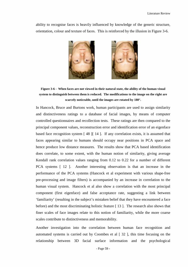
Literature Review
- Page 5599 --
ability to recognise faces is heavily influenced by knowledge of the generic structure,
orientation, colour and texture of faces. This is reinforced by the illusion in Figure 3-6.
Figure 3-6 - When faces are not viewed in their natural state, the ability of the human visual
system to distinguish between them is reduced. The modifications to the image on the right are
scarcely noticeable, until the images are rotated by 180°.
In Hancock, Bruce and Burtons work, human participants are used to assign similarity
and distinctiveness ratings to a database of facial images, by means of computer
controlled questionnaires and recollection tests. These ratings are then compared to the
principal component values, reconstruction error and identification error of an eigenface
based face recognition system [ 48 ][ 14 ]. If any correlation exists, it is assumed that
faces appearing similar to humans should occupy near positions in PCA space and
hence produce low distance measures. The results show that PCA based identification
does correlate, to some extent, with the human notion of similarity, giving average
Kendall rank correlation values ranging from 0.12 to 0.22 for a number of different
PCA systems [ 12 ]. Another interesting observation is that an increase in the
performance of the PCA systems (Hancock et al experiment with various shape-free
pre-processing and image filters) is accompanied by an increase in correlation to the
human visual system. Hancock et al also show a correlation with the most principal
component (first eigenface) and false acceptance rate, suggesting a link between
‘familiarity’ (resulting in the subject’s mistaken belief that they have encountered a face
before) and the most discriminating holistic feature [ 13 ]. The research also shows that
finer scales of face images relate to this notion of familiarity, while the more coarse
scales contribute to distinctiveness and memorability.
Another investigation into the correlation between human face recognition and
automated systems is carried out by Coombes et al [ 32 ], this time focusing on the
relationship between 3D facial surface information and the psychological
Literature Review
- Page 6600 --
distinctiveness of a face. Ten human judges were used to rate faces according to how
distinctive the facial image appeared to them. By comparing these distinctiveness
ratings with the 3D facial surface data, it was discovered (as one may have assumed)
that the more distinctive the face, the more the 3D facial surface deviated from the
average facial surface. In particular, the more distinctive faces were composed of fewer
flat surfaces in the lower regions of the facial surface.
33..55 SSuummmmaarr yy ooff PPeerr ffoorr mmaannccee
From the various papers described above, it is apparent that 2D face recognition has
achieved a reasonably high level of performance, particularly using the eigenface and
Fisherface appearance-based approaches. However, the error rates still being produced
by these systems do not seem to compare to the level that the human visual system is
able to discriminate between faces (although this statement is quite subjective). The
error rates are also still too high to be considered for many of the potential applications
of face recognition. We see that neural network approaches are well suited towards face
detection, which is a critical preliminary step to successful face recognition, but no
system has been presented which utilises the benefits offered by such a system prior to
any further verification or identification procedures. On a similar note, we have also
seen how feature analysis, although not accurate enough to perform a high level of
recognition of its own, could be used as a preliminary screening step.
Many researchers suggest that the main problem to be overcome by 2D face recognition
systems is that of lighting conditions. If this were to be achieved, face recognition
would become a much more attractive biometric for the purposes of verification for site
access. However, for face recognition to be used in a surveillance application, the
problem of facial expression and facial orientation must also be solved. Some attempts
have been made to combat both of these problems, with limited success. It is surprising
that image pre-processing, colour normalisation and lighting correction as used with
photo processing systems has not been applied more readily as a preliminary step to
appearance-based approaches (at most those explored use simple histogram equalisation
or brightness and contrast adjustment), as it is likely that such additional processing
could improve both the eigenface and Fisherface methods. Although Adini, Moses and
Ullman point out that there is no image representation that can be completely invariant
to lighting conditions, they do show that different representations of images, on which

Literature Review
- Page 6611 --
lighting has less of an affect, can significantly reduce the difference between two
images of the same face [ 26 ].
3D facial recognition has been identified as a viable biometric, with the potential for
high performance classification. However, very few 3D facial recognition systems have
been implemented and those that have been tested have only been applied to small
databases. Nevertheless, the results have all been promising. It is also evident that
subspace approaches could be equally applicable to 3D facial surface information,
although a large database of 3D face models is required to facilitate further research in
this area. The need for a common test database has been a recurring factor in many of
the papers discussed here and although the FRVT [ 1 ] and FERET database [ 44 ] have
gone some way to addressing these issues they are more often utilised in commercial
tests rather than adopted in research investigations and this makes cross-method
comparison very subjective. Some of the more common databases currently used for
2D face recognition are:
• The FERET database [ 41 ]
• The AR Face Database [ 39 ]
• The XM2VTS database. [ 66 ]
• The Psychological Image Collections at Sterling (PICS) [ 64 ]
• The UMIST Face Database [ 65 ]
• The Yale Face Database [ 67 ]
Although more researchers are beginning to make use of such databases for 2D face
recognition, the same problem can now be seen arising in the 3D field. Further
complicated by the greater variety of 3D data formats and the need for simultaneously
acquired 2D images. The Face Recognition Grand Challenge (FRGC) [ 2 ] does look
set to address some of these points, providing a defined testing methodology and 3D
face data with accompanying 2D images, although the database will not be available in
sufficient time for our own investigations and therefore we have had to address this
problem ourselves (see section 5.1).
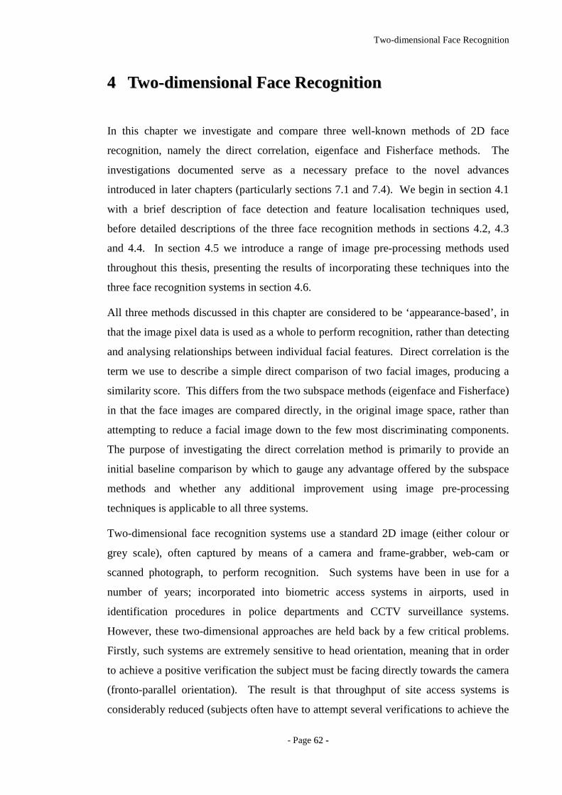
Two-dimensional Face Recognition
- Page 6622 --
44 TTwwoo--ddiimmeennssiioonnaall FFaaccee RReeccooggnnii tt iioonn
In this chapter we investigate and compare three well-known methods of 2D face
recognition, namely the direct correlation, eigenface and Fisherface methods. The
investigations documented serve as a necessary preface to the novel advances
introduced in later chapters (particularly sections 7.1 and 7.4). We begin in section 4.1
with a brief description of face detection and feature localisation techniques used,
before detailed descriptions of the three face recognition methods in sections 4.2, 4.3
and 4.4. In section 4.5 we introduce a range of image pre-processing methods used
throughout this thesis, presenting the results of incorporating these techniques into the
three face recognition systems in section 4.6.
All three methods discussed in this chapter are considered to be ‘appearance-based’, in
that the image pixel data is used as a whole to perform recognition, rather than detecting
and analysing relationships between individual facial features. Direct correlation is the
term we use to describe a simple direct comparison of two facial images, producing a
similarity score. This differs from the two subspace methods (eigenface and Fisherface)
in that the face images are compared directly, in the original image space, rather than
attempting to reduce a facial image down to the few most discriminating components.
The purpose of investigating the direct correlation method is primarily to provide an
initial baseline comparison by which to gauge any advantage offered by the subspace
methods and whether any additional improvement using image pre-processing
techniques is applicable to all three systems.
Two-dimensional face recognition systems use a standard 2D image (either colour or
grey scale), often captured by means of a camera and frame-grabber, web-cam or
scanned photograph, to perform recognition. Such systems have been in use for a
number of years; incorporated into biometric access systems in airports, used in
identification procedures in police departments and CCTV surveillance systems.
However, these two-dimensional approaches are held back by a few critical problems.
Firstly, such systems are extremely sensitive to head orientation, meaning that in order
to achieve a positive verification the subject must be facing directly towards the camera
(fronto-parallel orientation). The result is that throughput of site access systems is
considerably reduced (subjects often have to attempt several verifications to achieve the

Two-dimensional Face Recognition
- Page 6633 --
correct orientation) and surveillance systems rely on luck that the subject will face the
camera. The second major problem is lighting conditions. If the subject is enrolled in
an environment with different lighting conditions (including direction, intensity and
colour) to that when verification is performed, the subject is often falsely rejected.
In this chapter we explore three two-dimensional appearance-based methods of face
recognition, describing the theory and mathematical concepts behind each in sections
4.2, 4.3 and 4.4. We perform some preliminary experimentation using each of the three
methods on a small test set of facial images, providing an initial baseline indication of
how each system performs and the level of results that may be expected from such
experimentation. A more thorough comparison of the three systems on a common data
set is provided in section 4.6. For completeness sake, we also briefly cover the
necessary preliminary requirements of feature localisation in section 4.1. However, we
do not spend significant time researching or improving the method described,
considering it to be another topic worthy of further study in a separate project.
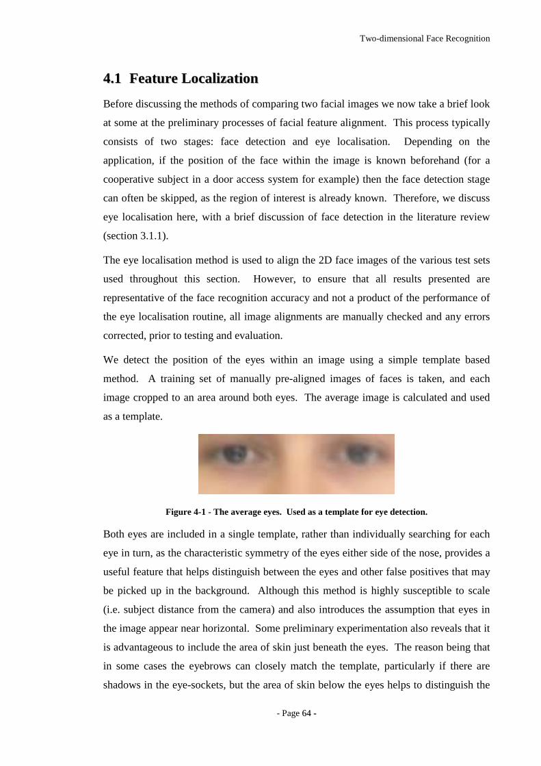
Two-dimensional Face Recognition
- Page 6644 --
44..11 FFeeaattuurr ee LL ooccaall iizzaatt iioonn
Before discussing the methods of comparing two facial images we now take a brief look
at some at the preliminary processes of facial feature alignment. This process typically
consists of two stages: face detection and eye localisation. Depending on the
application, if the position of the face within the image is known beforehand (for a
cooperative subject in a door access system for example) then the face detection stage
can often be skipped, as the region of interest is already known. Therefore, we discuss
eye localisation here, with a brief discussion of face detection in the literature review
(section 3.1.1).
The eye localisation method is used to align the 2D face images of the various test sets
used throughout this section. However, to ensure that all results presented are
representative of the face recognition accuracy and not a product of the performance of
the eye localisation routine, all image alignments are manually checked and any errors
corrected, prior to testing and evaluation.
We detect the position of the eyes within an image using a simple template based
method. A training set of manually pre-aligned images of faces is taken, and each
image cropped to an area around both eyes. The average image is calculated and used
as a template.
Figure 4-1 - The average eyes. Used as a template for eye detection.
Both eyes are included in a single template, rather than individually searching for each
eye in turn, as the characteristic symmetry of the eyes either side of the nose, provides a
useful feature that helps distinguish between the eyes and other false positives that may
be picked up in the background. Although this method is highly susceptible to scale
(i.e. subject distance from the camera) and also introduces the assumption that eyes in
the image appear near horizontal. Some preliminary experimentation also reveals that it
is advantageous to include the area of skin just beneath the eyes. The reason being that
in some cases the eyebrows can closely match the template, particularly if there are
shadows in the eye-sockets, but the area of skin below the eyes helps to distinguish the
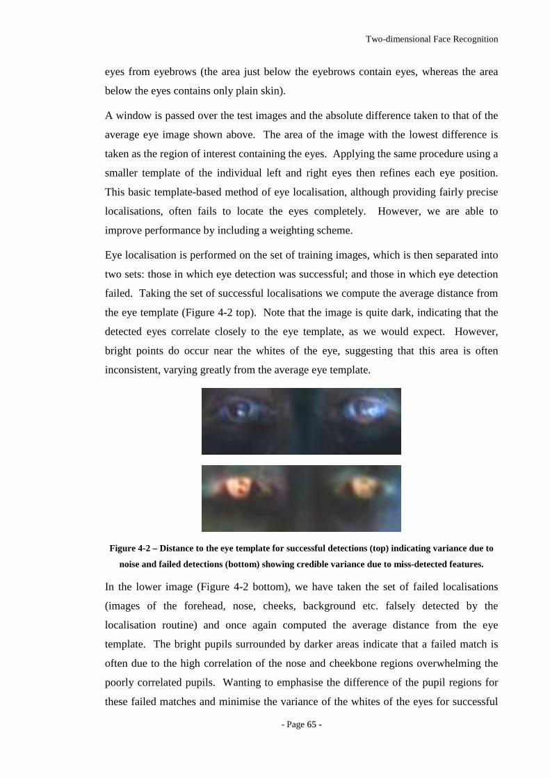
Two-dimensional Face Recognition
- Page 6655 --
eyes from eyebrows (the area just below the eyebrows contain eyes, whereas the area
below the eyes contains only plain skin).
A window is passed over the test images and the absolute difference taken to that of the
average eye image shown above. The area of the image with the lowest difference is
taken as the region of interest containing the eyes. Applying the same procedure using a
smaller template of the individual left and right eyes then refines each eye position.
This basic template-based method of eye localisation, although providing fairly precise
localisations, often fails to locate the eyes completely. However, we are able to
improve performance by including a weighting scheme.
Eye localisation is performed on the set of training images, which is then separated into
two sets: those in which eye detection was successful; and those in which eye detection
failed. Taking the set of successful localisations we compute the average distance from
the eye template (Figure 4-2 top). Note that the image is quite dark, indicating that the
detected eyes correlate closely to the eye template, as we would expect. However,
bright points do occur near the whites of the eye, suggesting that this area is often
inconsistent, varying greatly from the average eye template.
Figure 4-2 – Distance to the eye template for successful detections (top) indicating variance due to
noise and failed detections (bottom) showing credible variance due to miss-detected features.
In the lower image (Figure 4-2 bottom), we have taken the set of failed localisations
(images of the forehead, nose, cheeks, background etc. falsely detected by the
localisation routine) and once again computed the average distance from the eye
template. The bright pupils surrounded by darker areas indicate that a failed match is
often due to the high correlation of the nose and cheekbone regions overwhelming the
poorly correlated pupils. Wanting to emphasise the difference of the pupil regions for
these failed matches and minimise the variance of the whites of the eyes for successful
Two-dimensional Face Recognition
- Page 6666 --
matches, we divide the lower image values by the upper image to produce a weights
vector as shown in Figure 4-3. When applied to the difference image before summing a
total error, this weighting scheme provides a much improved detection rate.
Figure 4-3 - Eye template weights used to give higher priority to those pixels that best represent the
eyes.
44..22 TThhee DDii rr eecctt CCoorr rr eellaatt iioonn AApppprr ooaacchh
We begin our investigation into face recognition with perhaps the simplest approach,
known as the direct correlation method (also referred to as template matching by
Brunelli and Poggio [ 29 ]) involving the direct comparison of pixel intensity values
taken from facial images. We use the term ‘Direct Correlation’ to encompass all
techniques in which face images are compared directly, without any form of image
space analysis, weighting schemes or feature extraction, regardless of the distance
metric used. Therefore, we do not infer that Pearson’s correlation is applied as the
similarity function (although such an approach would obviously come under our
definition of direct correlation). We typically use the Euclidean distance as our metric
in these investigations (inversely related to Pearson’s correlation and can be considered
as a scale and translation sensitive form of image correlation), as this persists with the
contrast made between image space and subspace approaches in later sections.
Firstly, all facial images must be aligned such that the eye centres are located at two
specified pixel coordinates and the image cropped to remove any background
information. These images are stored as greyscale bitmaps of 65 by 82 pixels and prior
to recognition converted into a vector of 5330 elements (each element containing the
corresponding pixel intensity value). Each corresponding vector can be thought of as
describing a point within a 5330 dimensional image space. This simple principle can
easily be extended to much larger images: a 256 by 256 pixel image occupies a single
point in 65,536-dimensional image space and again, similar images occupy close points
within that space. Likewise, similar faces are located close together within the image
space, while dissimilar faces are spaced far apart. Calculating the Euclidean distance d,
Two-dimensional Face Recognition
- Page 6677 --
between two facial image vectors (often referred to as the query image q, and gallery
image g), we get an indication of similarity. A threshold is then applied to make the
final verification decision.
gqd −= )()( rejectthresholddacceptthresholdd ⇒>∧⇒≤ .
Equ. 4-1
4.2.1 Verification Tests
The primary concern in any face recognition system is its ability to correctly verify a
claimed identity or determine a person's most likely identity from a set of potential
matches in a database. In order to assess a given system’s ability to perform these tasks,
a variety of evaluation methodologies have arisen. Some of these analysis methods
simulate a specific mode of operation (i.e. secure site access or surveillance), while
others provide a more mathematical description of data distribution in some
classification space. In addition, the results generated from each analysis method may
be presented in a variety of formats.
Throughout the experimentations in this thesis, we primarily use the verification test as
our method of analysis and comparison, although we also use Fisher’s Linear
Discriminant to analyse individual subspace components in section 7 and the
identification test for the final evaluations described in section 8.
The verification test measures a system’s ability to correctly accept or reject the
proposed identity of an individual. At a functional level, this reduces to two images
being presented for comparison, for which the system must return either an acceptance
(the two images are of the same person) or rejection (the two images are of different
people). The test is designed to simulate the application area of secure site access. In
this scenario, a subject will present some form of identification at a point of entry,
perhaps as a swipe card, proximity chip or PIN number. This number is then used to
retrieve a stored image from a database of known subjects (often referred to as the target
or gallery image) and compared with a live image captured at the point of entry (the
query image). Access is then granted depending on the acceptance/rejection decision.
The results of the test are calculated according to how many times the accept/reject
decision is made correctly.

Two-dimensional Face Recognition
- Page 6688 --
In order to execute this test we must first define our test set of face images. Although
the number of images in the test set does not affect the results produced (as the error
rates are specified as percentages of image comparisons), it is important to ensure that
the test set is sufficiently large such that statistical anomalies become insignificant (for
example, a couple of badly aligned images matching well). Also, the type of images
(high variation in lighting, partial occlusions etc.) will significantly alter the results of
the test. Therefore, in order to compare multiple face recognition systems, they must be
applied to the same test set. However, it should also be noted that if the results are to be
representative of system performance in a real world situation, then the test data should
be captured under precisely the same circumstances as in the application environment.
On the other hand, if the purpose of the experimentation is to evaluate and improve a
method of face recognition, which may be applied to a range of application
environments, then the test data should present the range of difficulties that are to be
overcome. This may mean including a greater percentage of ‘difficult’ images than
would be expected in the perceived operating conditions and hence higher error rates in
the results produced.
Below we provide the algorithm for executing the verification test. The algorithm is
applied to a single test set of face images, using a single function call to the face
recognition algorithm: CompareFaces(FaceA, FaceB). This call is used to compare two
facial images, returning a distance score indicating how dissimilar the two face images
are: the lower the score the more similar the two face images. Ideally, images of the
same face should produce low scores, while images of different faces should produce
high scores.
Every image is compared with every other image, no image is compared with itself and
no pair is compared more than once (we assume that the relationship is symmetrical).
Once two images have been compared, producing a similarity score, the ground-truth is
used to determine if the images are of the same person or different people. In practical
tests this information is often encapsulated as part of the image filename (by means of a
unique person identifier). Scores are then stored in one of two lists: a list containing
scores produced by comparing images of different people and a list containing scores
produced by comparing images of the same person. The final acceptance/rejection
decision is made by application of a threshold. Any incorrect decision is recorded as
either a false acceptance or false rejection. The false rejection rate (FRR) is calculated
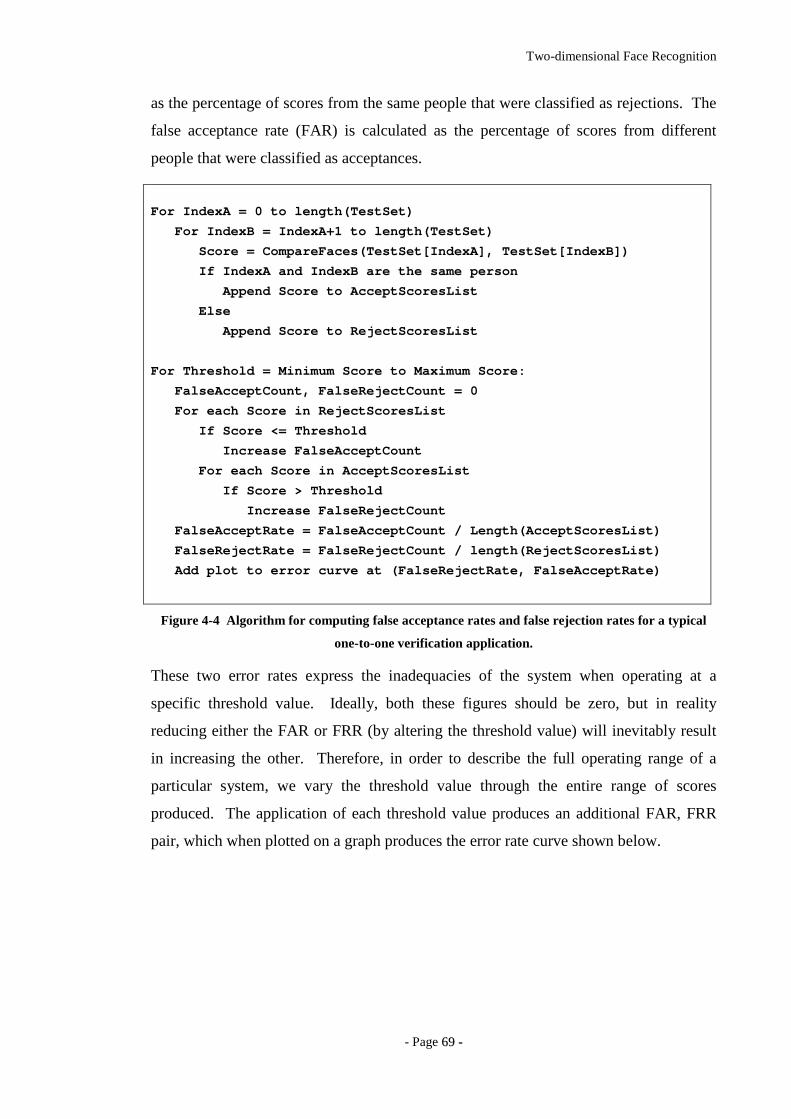
Two-dimensional Face Recognition
- Page 6699 --
as the percentage of scores from the same people that were classified as rejections. The
false acceptance rate (FAR) is calculated as the percentage of scores from different
people that were classified as acceptances.
For IndexA = 0 to length(TestSet)
For IndexB = IndexA+1 to length(TestSet)
Score = CompareFaces(TestSet[IndexA], TestSet [IndexB])
If IndexA and IndexB are the same person
Append Score to AcceptScoresList
Else
Append Score to RejectScoresList
For Threshold = Minimum Score to Maximum Score:
FalseAcceptCount, FalseRejectCount = 0
For each Score in RejectScoresList
If Score <= Threshold
Increase FalseAcceptCount
For each Score in AcceptScoresList
If Score > Threshold
Increase FalseRejectCount
FalseAcceptRate = FalseAcceptCount / Length(Acce ptScoresList)
FalseRejectRate = FalseRejectCount / length(Reje ctScoresList)
Add plot to error curve at (FalseRejectRate, Fal seAcceptRate)
Figure 4-4 Algorithm for computing false acceptance rates and false rejection rates for a typical
one-to-one verification application.
These two error rates express the inadequacies of the system when operating at a
specific threshold value. Ideally, both these figures should be zero, but in reality
reducing either the FAR or FRR (by altering the threshold value) will inevitably result
in increasing the other. Therefore, in order to describe the full operating range of a
particular system, we vary the threshold value through the entire range of scores
produced. The application of each threshold value produces an additional FAR, FRR
pair, which when plotted on a graph produces the error rate curve shown below.
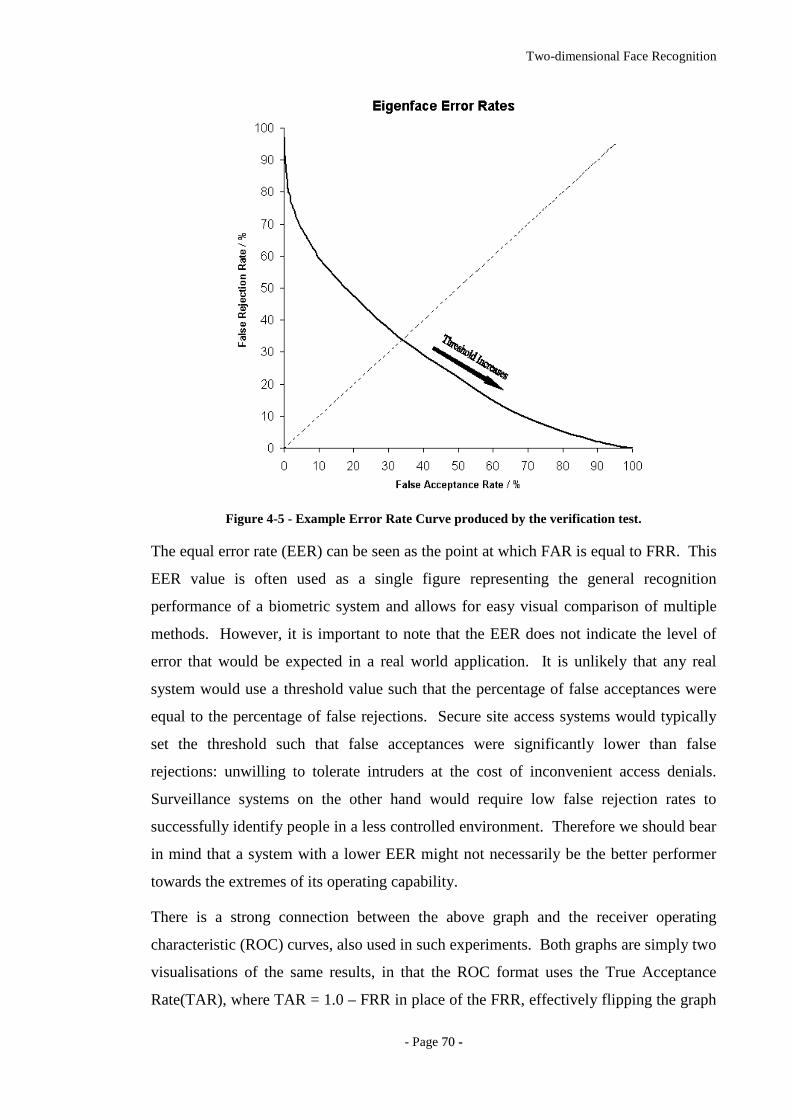
Two-dimensional Face Recognition
- Page 7700 --
Figure 4-5 - Example Error Rate Curve produced by the verification test.
The equal error rate (EER) can be seen as the point at which FAR is equal to FRR. This
EER value is often used as a single figure representing the general recognition
performance of a biometric system and allows for easy visual comparison of multiple
methods. However, it is important to note that the EER does not indicate the level of
error that would be expected in a real world application. It is unlikely that any real
system would use a threshold value such that the percentage of false acceptances were
equal to the percentage of false rejections. Secure site access systems would typically
set the threshold such that false acceptances were significantly lower than false
rejections: unwilling to tolerate intruders at the cost of inconvenient access denials.
Surveillance systems on the other hand would require low false rejection rates to
successfully identify people in a less controlled environment. Therefore we should bear
in mind that a system with a lower EER might not necessarily be the better performer
towards the extremes of its operating capability.
There is a strong connection between the above graph and the receiver operating
characteristic (ROC) curves, also used in such experiments. Both graphs are simply two
visualisations of the same results, in that the ROC format uses the True Acceptance
Rate(TAR), where TAR = 1.0 – FRR in place of the FRR, effectively flipping the graph
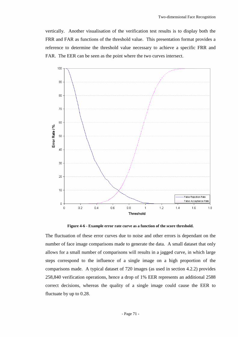
Two-dimensional Face Recognition
- Page 7711 --
vertically. Another visualisation of the verification test results is to display both the
FRR and FAR as functions of the threshold value. This presentation format provides a
reference to determine the threshold value necessary to achieve a specific FRR and
FAR. The EER can be seen as the point where the two curves intersect.
Figure 4-6 - Example error rate curve as a function of the score threshold.
The fluctuation of these error curves due to noise and other errors is dependant on the
number of face image comparisons made to generate the data. A small dataset that only
allows for a small number of comparisons will results in a jagged curve, in which large
steps correspond to the influence of a single image on a high proportion of the
comparisons made. A typical dataset of 720 images (as used in section 4.2.2) provides
258,840 verification operations, hence a drop of 1% EER represents an additional 2588
correct decisions, whereas the quality of a single image could cause the EER to
fluctuate by up to 0.28.
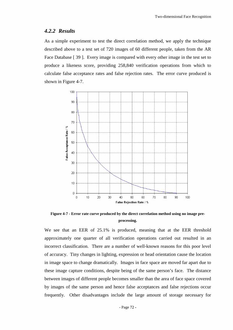
Two-dimensional Face Recognition
- Page 7722 --
4.2.2 Results
As a simple experiment to test the direct correlation method, we apply the technique
described above to a test set of 720 images of 60 different people, taken from the AR
Face Database [ 39 ]. Every image is compared with every other image in the test set to
produce a likeness score, providing 258,840 verification operations from which to
calculate false acceptance rates and false rejection rates. The error curve produced is
shown in Figure 4-7.
Figure 4-7 - Error rate curve produced by the direct correlation method using no image pre-
processing.
We see that an EER of 25.1% is produced, meaning that at the EER threshold
approximately one quarter of all verification operations carried out resulted in an
incorrect classification. There are a number of well-known reasons for this poor level
of accuracy. Tiny changes in lighting, expression or head orientation cause the location
in image space to change dramatically. Images in face space are moved far apart due to
these image capture conditions, despite being of the same person’s face. The distance
between images of different people becomes smaller than the area of face space covered
by images of the same person and hence false acceptances and false rejections occur
frequently. Other disadvantages include the large amount of storage necessary for

Two-dimensional Face Recognition
- Page 7733 --
holding many face images and the intensive processing required for each comparison,
making this method unsuitable for applications applied to a large database. In section
4.3 we explore the eigenface method, which attempts to address some of these issues.
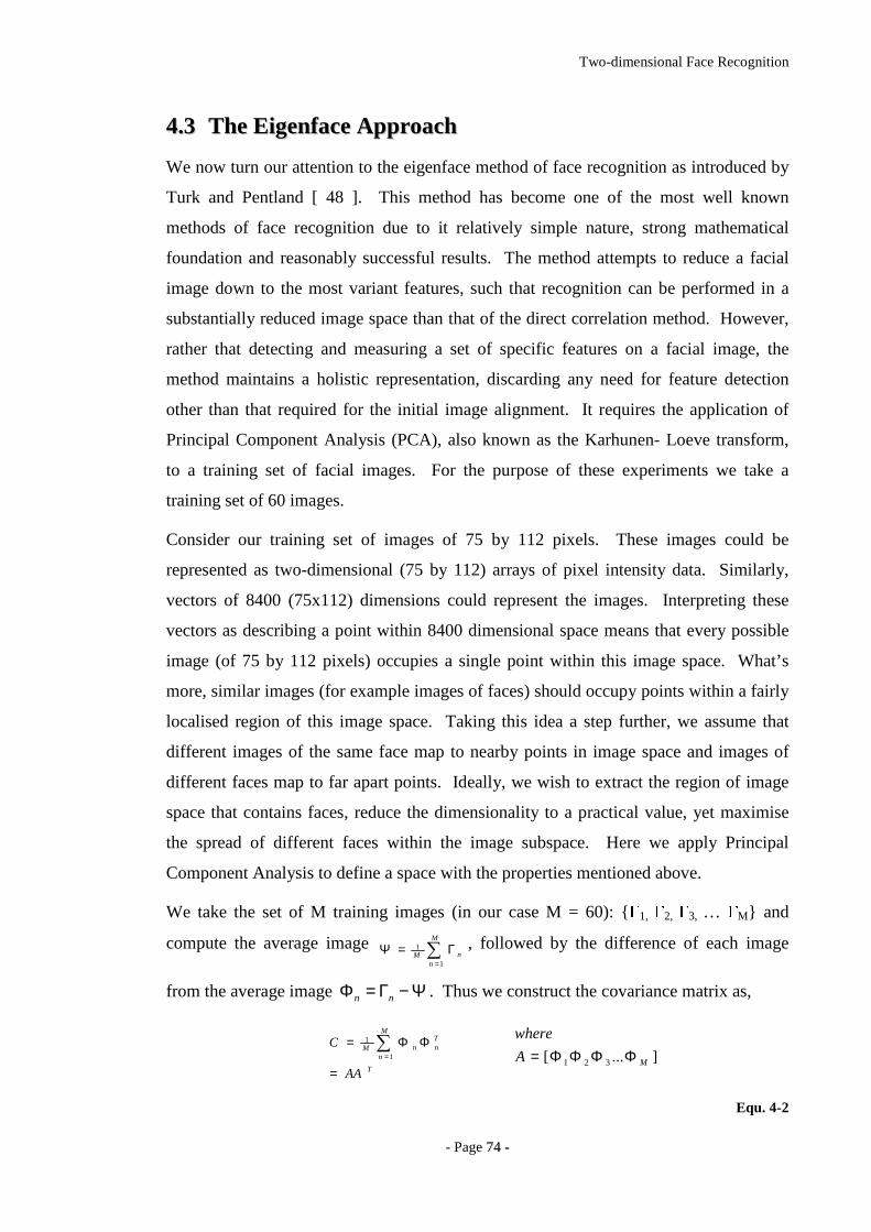
Two-dimensional Face Recognition
- Page 7744 --
44..33 TThhee EEiiggeennffaaccee AApppprr ooaacchh
We now turn our attention to the eigenface method of face recognition as introduced by
Turk and Pentland [ 48 ]. This method has become one of the most well known
methods of face recognition due to it relatively simple nature, strong mathematical
foundation and reasonably successful results. The method attempts to reduce a facial
image down to the most variant features, such that recognition can be performed in a
substantially reduced image space than that of the direct correlation method. However,
rather that detecting and measuring a set of specific features on a facial image, the
method maintains a holistic representation, discarding any need for feature detection
other than that required for the initial image alignment. It requires the application of
Principal Component Analysis (PCA), also known as the Karhunen- Loeve transform,
to a training set of facial images. For the purpose of these experiments we take a
training set of 60 images.
Consider our training set of images of 75 by 112 pixels. These images could be
represented as two-dimensional (75 by 112) arrays of pixel intensity data. Similarly,
vectors of 8400 (75x112) dimensions could represent the images. Interpreting these
vectors as describing a point within 8400 dimensional space means that every possible
image (of 75 by 112 pixels) occupies a single point within this image space. What’s
more, similar images (for example images of faces) should occupy points within a fairly
localised region of this image space. Taking this idea a step further, we assume that
different images of the same face map to nearby points in image space and images of
different faces map to far apart points. Ideally, we wish to extract the region of image
space that contains faces, reduce the dimensionality to a practical value, yet maximise
the spread of different faces within the image subspace. Here we apply Principal
Component Analysis to define a space with the properties mentioned above.
We take the set of M training images (in our case M = 60): 1, 2, 3, … M and
compute the average image ∑=
Γ=ΨM
nnM
1
1 , followed by the difference of each image
from the average image Ψ−Γ=Φ nn . Thus we construct the covariance matrix as,
T
M
n
TnnM
AA
C
=
ΦΦ= ∑=1
1 ]...[ 321 MA
where
ΦΦΦΦ=
Equ. 4-2
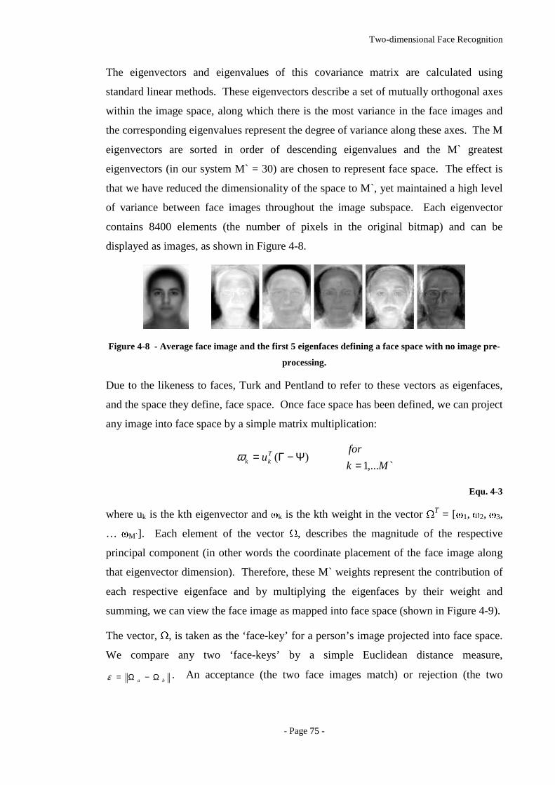
Two-dimensional Face Recognition
- Page 7755 --
The eigenvectors and eigenvalues of this covariance matrix are calculated using
standard linear methods. These eigenvectors describe a set of mutually orthogonal axes
within the image space, along which there is the most variance in the face images and
the corresponding eigenvalues represent the degree of variance along these axes. The M
eigenvectors are sorted in order of descending eigenvalues and the M` greatest
eigenvectors (in our system M` = 30) are chosen to represent face space. The effect is
that we have reduced the dimensionality of the space to M`, yet maintained a high level
of variance between face images throughout the image subspace. Each eigenvector
contains 8400 elements (the number of pixels in the original bitmap) and can be
displayed as images, as shown in Figure 4-8.
Figure 4-8 - Average face image and the first 5 eigenfaces defining a face space with no image pre-
processing.
Due to the likeness to faces, Turk and Pentland to refer to these vectors as eigenfaces,
and the space they define, face space. Once face space has been defined, we can project
any image into face space by a simple matrix multiplication:
)( Ψ−Γ= Tkk uω
`,...1 Mk
for
=
Equ. 4-3
where uk is the kth eigenvector and k is the kth weight in the vector T = [1, 2, 3,
… M`]. Each element of the vector
, describes the magnitude of the respective
principal component (in other words the coordinate placement of the face image along
that eigenvector dimension). Therefore, these M` weights represent the contribution of
each respective eigenface and by multiplying the eigenfaces by their weight and
summing, we can view the face image as mapped into face space (shown in Figure 4-9).
The vector,
, is taken as the ‘face-key’ for a person’s image projected into face space.
We compare any two ‘face-keys’ by a simple Euclidean distance measure,
ba Ω−Ω=ε . An acceptance (the two face images match) or rejection (the two
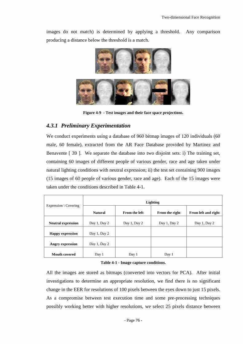
Two-dimensional Face Recognition
- Page 7766 --
images do not match) is determined by applying a threshold. Any comparison
producing a distance below the threshold is a match.
Figure 4-9 - Test images and their face space projections.
4.3.1 Preliminary Experimentation
We conduct experiments using a database of 960 bitmap images of 120 individuals (60
male, 60 female), extracted from the AR Face Database provided by Martinez and
Benavente [ 39 ]. We separate the database into two disjoint sets: i) The training set,
containing 60 images of different people of various gender, race and age taken under
natural lighting conditions with neutral expression; ii) the test set containing 900 images
(15 images of 60 people of various gender, race and age). Each of the 15 images were
taken under the conditions described in Table 4-1.
Lighting Expression \ Covering
Natural From the left From the right From left and right
Neutral expression Day 1, Day 2 Day 1, Day 2 Day 1, Day 2 Day 1, Day 2
Happy expression Day 1, Day 2
Angry expression Day 1, Day 2
Mouth covered Day 1 Day 1 Day 1
Table 4-1 - Image capture conditions.
All the images are stored as bitmaps (converted into vectors for PCA). After initial
investigations to determine an appropriate resolution, we find there is no significant
change in the EER for resolutions of 100 pixels between the eyes down to just 15 pixels.
As a compromise between test execution time and some pre-processing techniques
possibly working better with higher resolutions, we select 25 pixels distance between
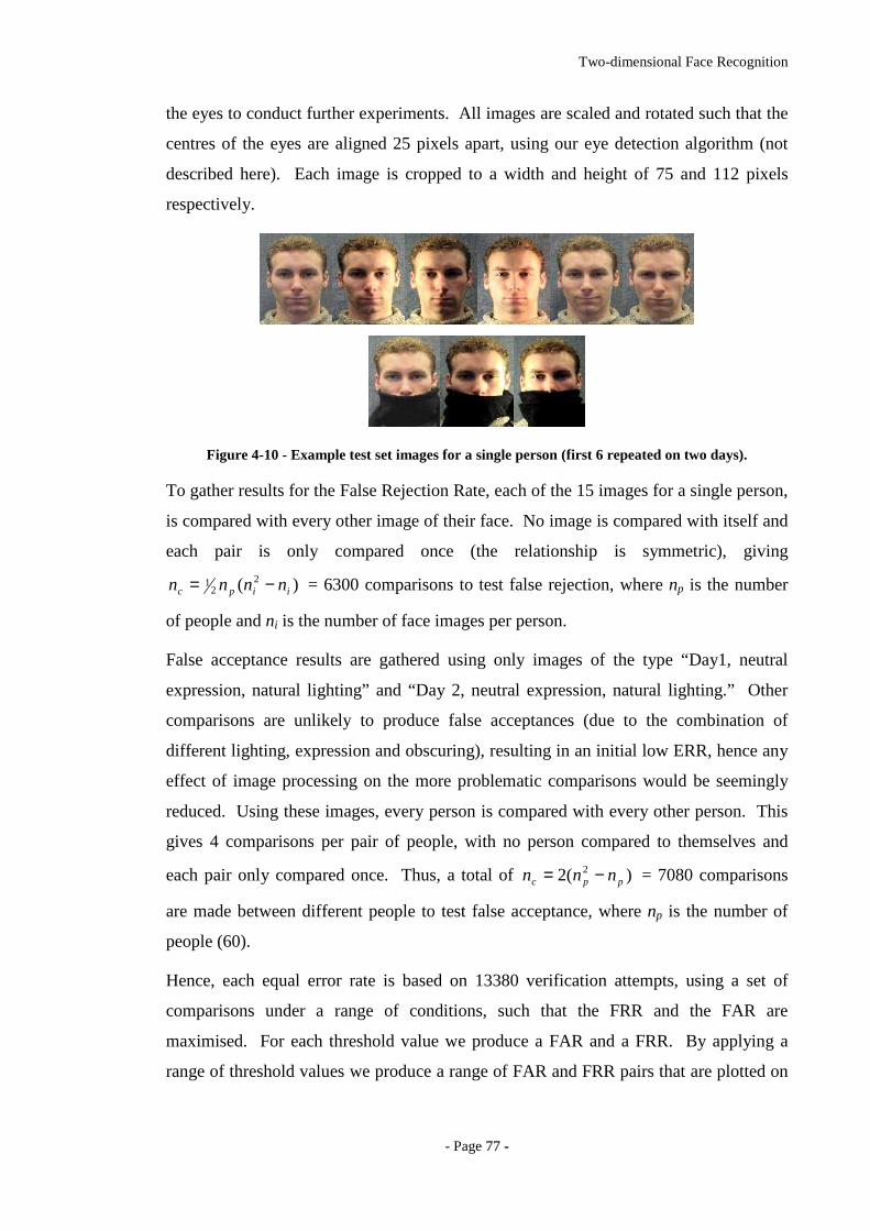
Two-dimensional Face Recognition
- Page 7777 --
the eyes to conduct further experiments. All images are scaled and rotated such that the
centres of the eyes are aligned 25 pixels apart, using our eye detection algorithm (not
described here). Each image is cropped to a width and height of 75 and 112 pixels
respectively.
Figure 4-10 - Example test set images for a single person (first 6 repeated on two days).
To gather results for the False Rejection Rate, each of the 15 images for a single person,
is compared with every other image of their face. No image is compared with itself and
each pair is only compared once (the relationship is symmetric), giving
)( 22
1iipc nnnn −= = 6300 comparisons to test false rejection, where np is the number
of people and ni is the number of face images per person.
False acceptance results are gathered using only images of the type “Day1, neutral
expression, natural lighting” and “Day 2, neutral expression, natural lighting.” Other
comparisons are unlikely to produce false acceptances (due to the combination of
different lighting, expression and obscuring), resulting in an initial low ERR, hence any
effect of image processing on the more problematic comparisons would be seemingly
reduced. Using these images, every person is compared with every other person. This
gives 4 comparisons per pair of people, with no person compared to themselves and
each pair only compared once. Thus, a total of )(2 2ppc nnn −= = 7080 comparisons
are made between different people to test false acceptance, where np is the number of
people (60).
Hence, each equal error rate is based on 13380 verification attempts, using a set of
comparisons under a range of conditions, such that the FRR and the FAR are
maximised. For each threshold value we produce a FAR and a FRR. By applying a
range of threshold values we produce a range of FAR and FRR pairs that are plotted on
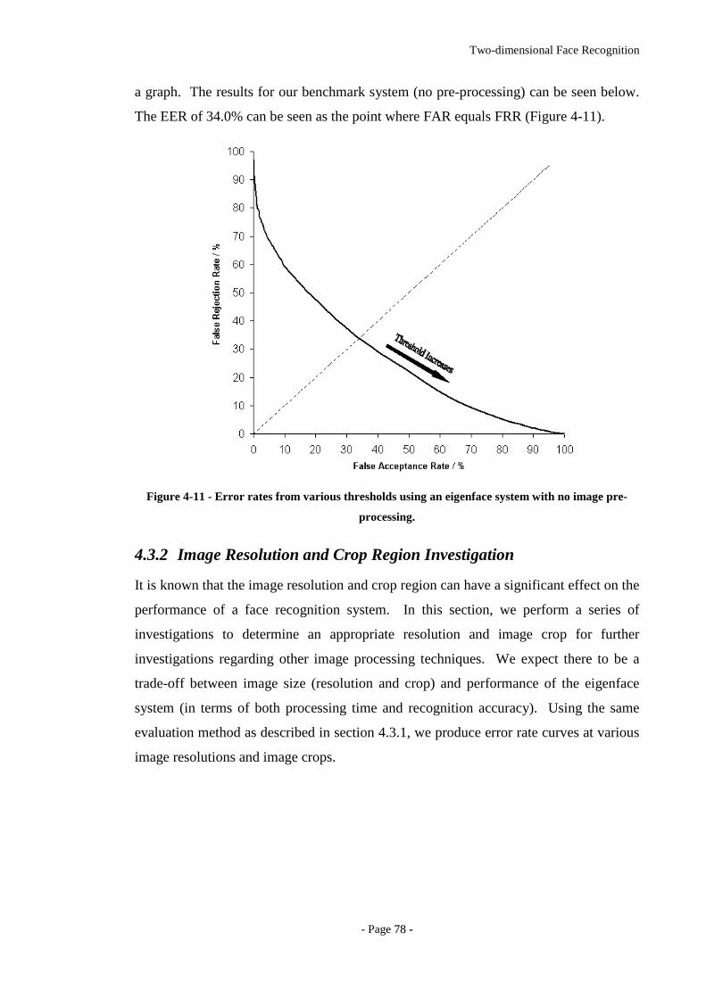
Two-dimensional Face Recognition
- Page 7788 --
a graph. The results for our benchmark system (no pre-processing) can be seen below.
The EER of 34.0% can be seen as the point where FAR equals FRR (Figure 4-11).
Figure 4-11 - Error rates from various thresholds using an eigenface system with no image pre-
processing.
4.3.2 Image Resolution and Crop Region Investigation
It is known that the image resolution and crop region can have a significant effect on the
performance of a face recognition system. In this section, we perform a series of
investigations to determine an appropriate resolution and image crop for further
investigations regarding other image processing techniques. We expect there to be a
trade-off between image size (resolution and crop) and performance of the eigenface
system (in terms of both processing time and recognition accuracy). Using the same
evaluation method as described in section 4.3.1, we produce error rate curves at various
image resolutions and image crops.
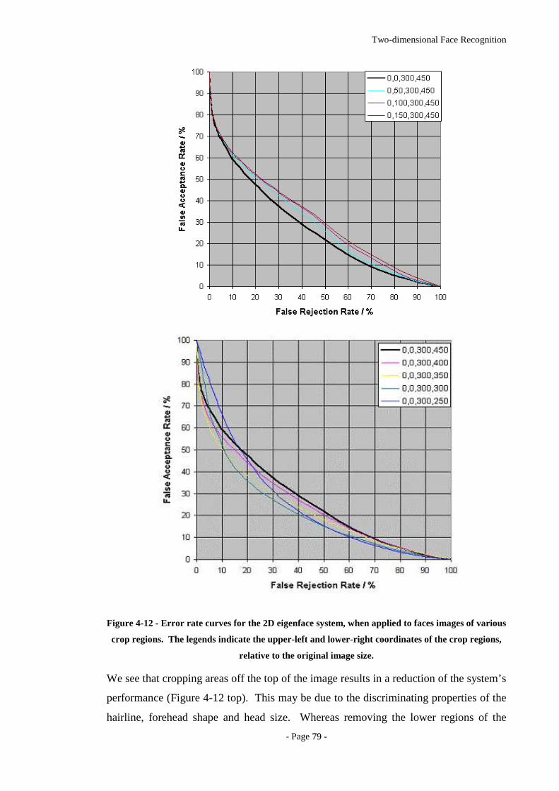
Two-dimensional Face Recognition
- Page 7799 --
Figure 4-12 - Error rate curves for the 2D eigenface system, when applied to faces images of various
crop regions. The legends indicate the upper-left and lower-right coordinates of the crop regions,
relative to the original image size.
We see that cropping areas off the top of the image results in a reduction of the system’s
performance (Figure 4-12 top). This may be due to the discriminating properties of the
hairline, forehead shape and head size. Whereas removing the lower regions of the

Two-dimensional Face Recognition
- Page 8800 --
image seems to have a positive impact on the systems error rates (Figure 4-12 bottom).
This is most likely due to the mouth area being the most flexible part of the face, which
changes most dramatically with different facial expressions. Despite these
improvements, we decide to keep the original area of the image, without applying any
cropping. Although we have demonstrated that the crop region significantly affects the
error rates, and indeed the error rate could be improved by removing the lower regions
of the face, it is our goal to overcome these problems by creating a more discriminating
image representation. If such a representation is found, the lower regions of the face
may begin to provide a positive contribution to the system performance. Once the best
image pre-processing method has been found, we can then test various crop regions
again, for any further improvement in performance (see section 5.1.2).

Two-dimensional Face Recognition
- Page 8811 --
Figure 4-13 - Error rate curves for the 2D eigenface system, when applied to faces images of various
resolutions. The graph on the right shows the region between 33.5% and 34.5% error rates of the
graph on the left.
Two-dimensional Face Recognition
- Page 8822 --
We find there is no significant change in the EER for resolutions of 100 pixels between
the eyes down to just 10 pixels (from 34.1 percent, down to 33.9 percent). Even more
surprising, is that the reduction in resolution appears to actually improve the system’s
performance (although only by a small degree). This may be due to the smoothing and
noise reduction side effects of the sub-sampling algorithm. As a compromise between
test execution time and some pre-processing techniques possibly working better with
higher resolutions, we select 25 pixels distance between the eyes to conduct all further
experiments. All images are scaled and rotated such that the centres of the eyes are
aligned 25 pixels apart, using our eye detection algorithm (see section 4.1.1). Each
image has a width and height of 75 and 112 pixels respectively.
4.3.3 Image Pre-processing Results
Various image pre-processing methods are often said to aid face recognition by
normalising various environmental influences, reducing noise or making distinguishing
features more explicit. For example edge detection techniques are thought to improve a
face recognition systems ability to cope with variations in lighting conditions (by
reducing an image to the shape and position of edges alone, rather than the colour and
texture of the face). On the other hand, colour normalisation methods may improve
recognition by trying to extract the ‘true colour’ of facial regions, regardless of lighting
conditions. Smoothing and blurring techniques can help by reducing noise from the
camera CCD and may also offer some resistance to small movements, rotations and
expression changes.
All of these image pre-processing techniques produce very different effects on face
images, and depending on the circumstances in which a system is expected to operate,
may either help or hinder performance. What’s more, there is surprisingly little
literature exploring how image-processing effects differ across the three variations of
appearance-based approaches discussed here. With such a variety of image processing
methods and a variety of reasons why each may improve performance, we are motivated
to test a large range of standard techniques.
Having tested the baseline eigenface system on raw image data and identified a suitable
resolution at which to conduct further investigations, in order to ascertain the effects of
image pre-processing, we now present results for a range of image processing
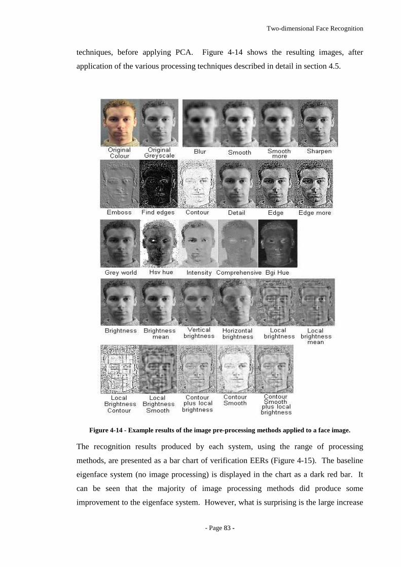
Two-dimensional Face Recognition
- Page 8833 --
techniques, before applying PCA. Figure 4-14 shows the resulting images, after
application of the various processing techniques described in detail in section 4.5.
Figure 4-14 - Example results of the image pre-processing methods applied to a face image.
The recognition results produced by each system, using the range of processing
methods, are presented as a bar chart of verification EERs (Figure 4-15). The baseline
eigenface system (no image processing) is displayed in the chart as a dark red bar. It
can be seen that the majority of image processing methods did produce some
improvement to the eigenface system. However, what is surprising is the large increase
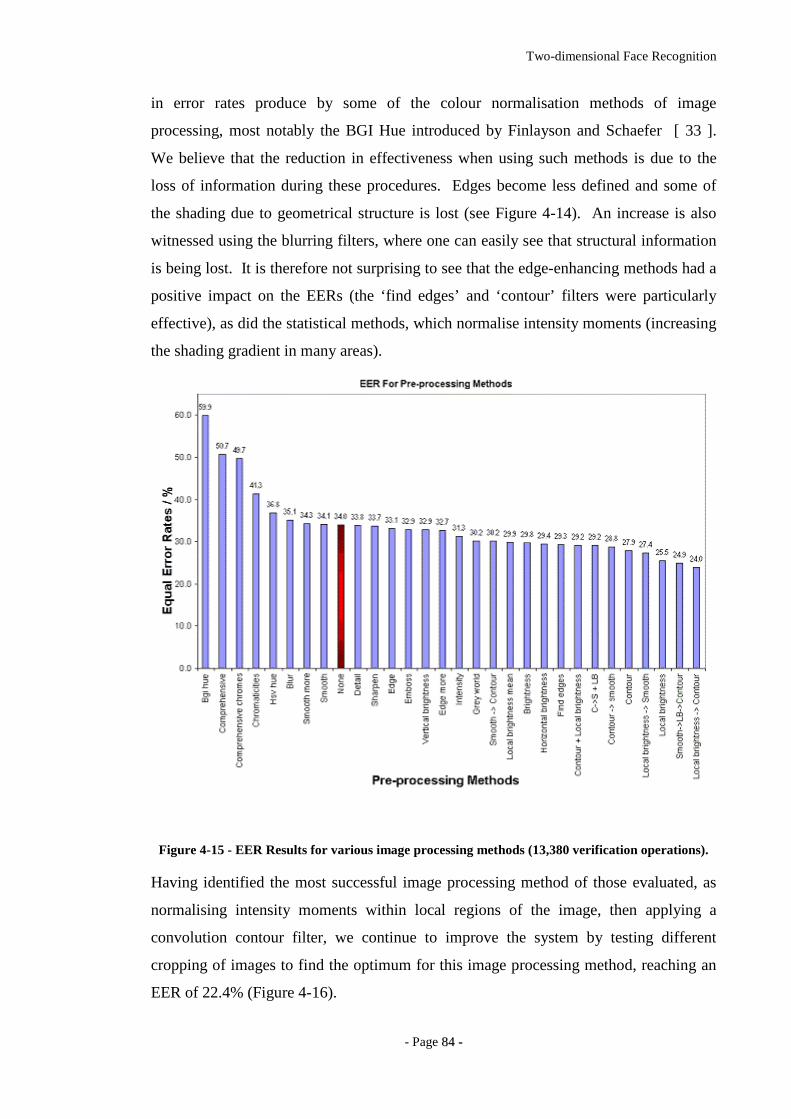
Two-dimensional Face Recognition
- Page 8844 --
in error rates produce by some of the colour normalisation methods of image
processing, most notably the BGI Hue introduced by Finlayson and Schaefer [ 33 ].
We believe that the reduction in effectiveness when using such methods is due to the
loss of information during these procedures. Edges become less defined and some of
the shading due to geometrical structure is lost (see Figure 4-14). An increase is also
witnessed using the blurring filters, where one can easily see that structural information
is being lost. It is therefore not surprising to see that the edge-enhancing methods had a
positive impact on the EERs (the ‘find edges’ and ‘contour’ filters were particularly
effective), as did the statistical methods, which normalise intensity moments (increasing
the shading gradient in many areas).
Figure 4-15 - EER Results for various image processing methods (13,380 verification operations).
Having identified the most successful image processing method of those evaluated, as
normalising intensity moments within local regions of the image, then applying a
convolution contour filter, we continue to improve the system by testing different
cropping of images to find the optimum for this image processing method, reaching an
EER of 22.4% (Figure 4-16).
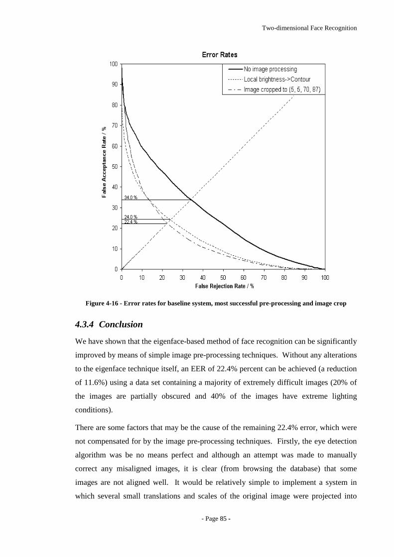
Two-dimensional Face Recognition
- Page 8855 --
Figure 4-16 - Error rates for baseline system, most successful pre-processing and image crop
4.3.4 Conclusion
We have shown that the eigenface-based method of face recognition can be significantly
improved by means of simple image pre-processing techniques. Without any alterations
to the eigenface technique itself, an EER of 22.4% percent can be achieved (a reduction
of 11.6%) using a data set containing a majority of extremely difficult images (20% of
the images are partially obscured and 40% of the images have extreme lighting
conditions).
There are some factors that may be the cause of the remaining 22.4% error, which were
not compensated for by the image pre-processing techniques. Firstly, the eye detection
algorithm was be no means perfect and although an attempt was made to manually
correct any misaligned images, it is clear (from browsing the database) that some
images are not aligned well. It would be relatively simple to implement a system in
which several small translations and scales of the original image were projected into

Two-dimensional Face Recognition
- Page 8866 --
face space for each recognition attempt (taking the lowest distance value returned),
hence compensating for any inaccuracies in the alignment procedure.
Comparable EER reductions have been witnessed in similar PCA methods of face
recognition, such as Pentland et al’s modular eigenspace system [ 40 ] and in
Belhumeur et al’s comparison to Fisher faces [ 27 ]. It is likely that the image pre-
processing methods described could be of similar benefit to these algorithms, and result
in a greatly improved face recognition system.
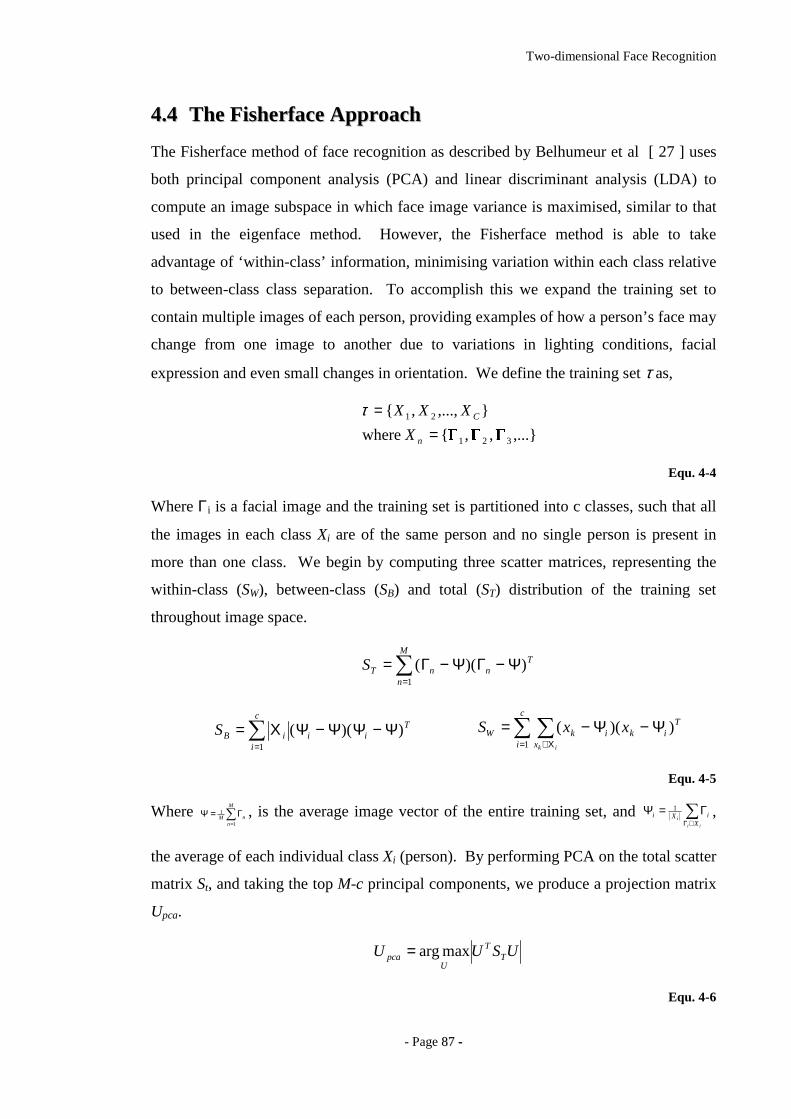
Two-dimensional Face Recognition
- Page 8877 --
44..44 TThhee FFiisshheerr ffaaccee AApppprr ooaacchh
The Fisherface method of face recognition as described by Belhumeur et al [ 27 ] uses
both principal component analysis (PCA) and linear discriminant analysis (LDA) to
compute an image subspace in which face image variance is maximised, similar to that
used in the eigenface method. However, the Fisherface method is able to take
advantage of ‘within-class’ information, minimising variation within each class relative
to between-class class separation. To accomplish this we expand the training set to
contain multiple images of each person, providing examples of how a person’s face may
change from one image to another due to variations in lighting conditions, facial
expression and even small changes in orientation. We define the training set τ as,
,...,, where
,...,,
321
21 =
=
n
C
X
XXXτ
Equ. 4-4
Where Γi is a facial image and the training set is partitioned into c classes, such that all
the images in each class Xi are of the same person and no single person is present in
more than one class. We begin by computing three scatter matrices, representing the
within-class (SW), between-class (SB) and total (ST) distribution of the training set
throughout image space.
∑=
Ψ−ΓΨ−Γ=M
n
TnnTS
1
))((
∑=
Ψ−ΨΨ−ΨΧ=c
i
TiiiBS
1
))((
∑ ∑= Χ∈
Ψ−Ψ−=c
i x
TikikW
ik
xxS1
))((
Equ. 4-5
Where ∑=
Γ=ΨM
nnM
1
1 , is the average image vector of the entire training set, and ∑∈Γ
Γ=Ψii
iX
iXi1 ,
the average of each individual class Xi (person). By performing PCA on the total scatter
matrix St, and taking the top M-c principal components, we produce a projection matrix
Upca.
USUU TT
Upca maxarg=
Equ. 4-6
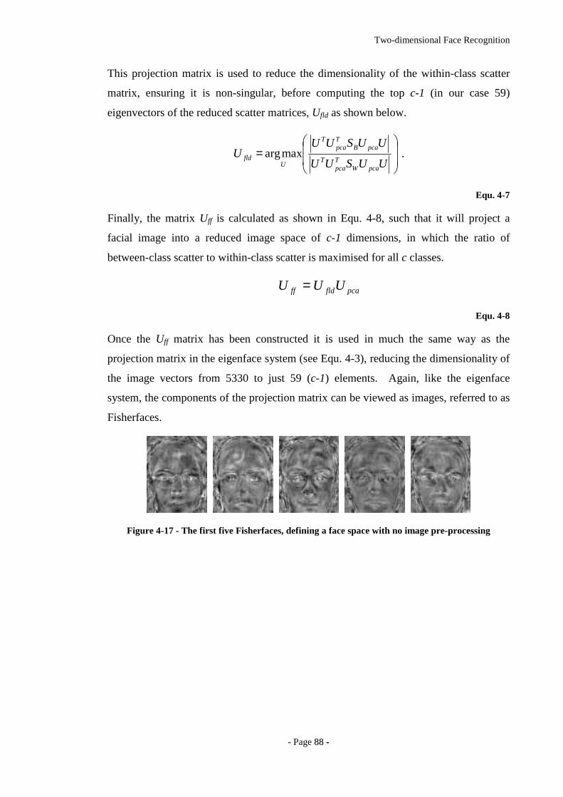
Two-dimensional Face Recognition
- Page 8888 --
This projection matrix is used to reduce the dimensionality of the within-class scatter
matrix, ensuring it is non-singular, before computing the top c-1 (in our case 59)
eigenvectors of the reduced scatter matrices, Ufld as shown below.
. maxarg
=
UUSUU
UUSUUU
pcaWTpca
T
pcaBTpca
T
Ufld
Equ. 4-7
Finally, the matrix Uff is calculated as shown in Equ. 4-8, such that it will project a
facial image into a reduced image space of c-1 dimensions, in which the ratio of
between-class scatter to within-class scatter is maximised for all c classes.
pcafldff UUU =
Equ. 4-8
Once the Uff matrix has been constructed it is used in much the same way as the
projection matrix in the eigenface system (see Equ. 4-3), reducing the dimensionality of
the image vectors from 5330 to just 59 (c-1) elements. Again, like the eigenface
system, the components of the projection matrix can be viewed as images, referred to as
Fisherfaces.
Figure 4-17 - The first five Fisherfaces, defining a face space with no image pre-processing
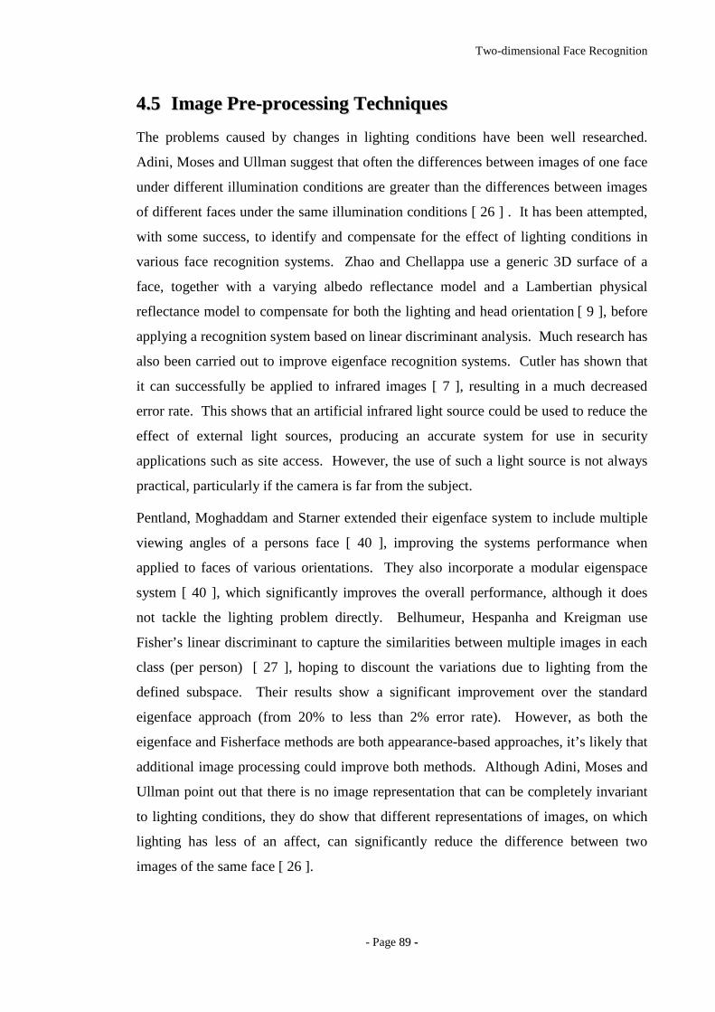
Two-dimensional Face Recognition
- Page 8899 --
44..55 II mmaaggee PPrr ee--pprr oocceessssiinngg TTeecchhnniiqquueess
The problems caused by changes in lighting conditions have been well researched.
Adini, Moses and Ullman suggest that often the differences between images of one face
under different illumination conditions are greater than the differences between images
of different faces under the same illumination conditions [ 26 ] . It has been attempted,
with some success, to identify and compensate for the effect of lighting conditions in
various face recognition systems. Zhao and Chellappa use a generic 3D surface of a
face, together with a varying albedo reflectance model and a Lambertian physical
reflectance model to compensate for both the lighting and head orientation [ 9 ], before
applying a recognition system based on linear discriminant analysis. Much research has
also been carried out to improve eigenface recognition systems. Cutler has shown that
it can successfully be applied to infrared images [ 7 ], resulting in a much decreased
error rate. This shows that an artificial infrared light source could be used to reduce the
effect of external light sources, producing an accurate system for use in security
applications such as site access. However, the use of such a light source is not always
practical, particularly if the camera is far from the subject.
Pentland, Moghaddam and Starner extended their eigenface system to include multiple
viewing angles of a persons face [ 40 ], improving the systems performance when
applied to faces of various orientations. They also incorporate a modular eigenspace
system [ 40 ], which significantly improves the overall performance, although it does
not tackle the lighting problem directly. Belhumeur, Hespanha and Kreigman use
Fisher’s linear discriminant to capture the similarities between multiple images in each
class (per person) [ 27 ], hoping to discount the variations due to lighting from the
defined subspace. Their results show a significant improvement over the standard
eigenface approach (from 20% to less than 2% error rate). However, as both the
eigenface and Fisherface methods are both appearance-based approaches, it’s likely that
additional image processing could improve both methods. Although Adini, Moses and
Ullman point out that there is no image representation that can be completely invariant
to lighting conditions, they do show that different representations of images, on which
lighting has less of an affect, can significantly reduce the difference between two
images of the same face [ 26 ].
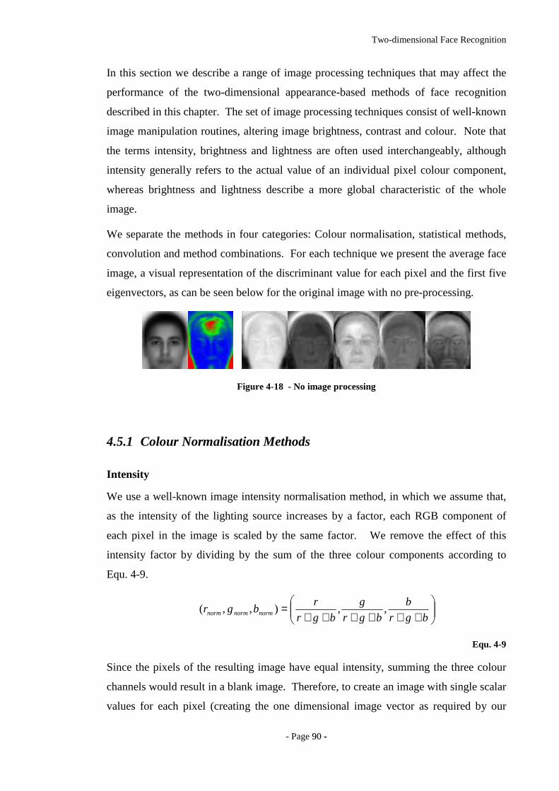
Two-dimensional Face Recognition
- Page 9900 --
In this section we describe a range of image processing techniques that may affect the
performance of the two-dimensional appearance-based methods of face recognition
described in this chapter. The set of image processing techniques consist of well-known
image manipulation routines, altering image brightness, contrast and colour. Note that
the terms intensity, brightness and lightness are often used interchangeably, although
intensity generally refers to the actual value of an individual pixel colour component,
whereas brightness and lightness describe a more global characteristic of the whole
image.
We separate the methods in four categories: Colour normalisation, statistical methods,
convolution and method combinations. For each technique we present the average face
image, a visual representation of the discriminant value for each pixel and the first five
eigenvectors, as can be seen below for the original image with no pre-processing.
Figure 4-18 - No image processing
4.5.1 Colour Normalisation Methods
Intensity
We use a well-known image intensity normalisation method, in which we assume that,
as the intensity of the lighting source increases by a factor, each RGB component of
each pixel in the image is scaled by the same factor. We remove the effect of this
intensity factor by dividing by the sum of the three colour components according to
Equ. 4-9.
++++++=
bgr
b
bgr
g
bgr
rbgr normnormnorm ,,),,(
Equ. 4-9
Since the pixels of the resulting image have equal intensity, summing the three colour
channels would result in a blank image. Therefore, to create an image with single scalar
values for each pixel (creating the one dimensional image vector as required by our
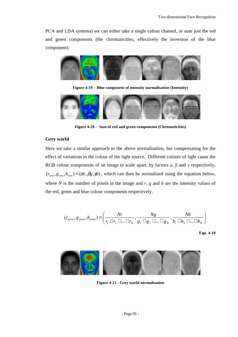
Two-dimensional Face Recognition
- Page 9911 --
PCA and LDA systems) we can either take a single colour channel, or sum just the red
and green components (the chromaticities, effectively the inversion of the blue
component).
Figure 4-19 - Blue component of intensity normalisation (Intensity)
Figure 4-20 - Sum of red and green components (Chromaticities)
Grey world
Here we take a similar approach to the above normalisation, but compensating for the
effect of variations in the colour of the light source. Different colours of light cause the
RGB colour components of an image to scale apart, by factors , and respectively,
),,(),,( bgrbgr newnewnew γβα= , which can then be normalised using the equation below,
where N is the number of pixels in the image and r, g and b are the intensity values of
the red, green and blue colour components respectively.
+++++++++=
NNNnormnormnorm bbb
Nb
ggg
Ng
rrr
Nrbgr
...,
...,
...),,(
212121
Equ. 4-10
Figure 4-21 - Grey world normalisation
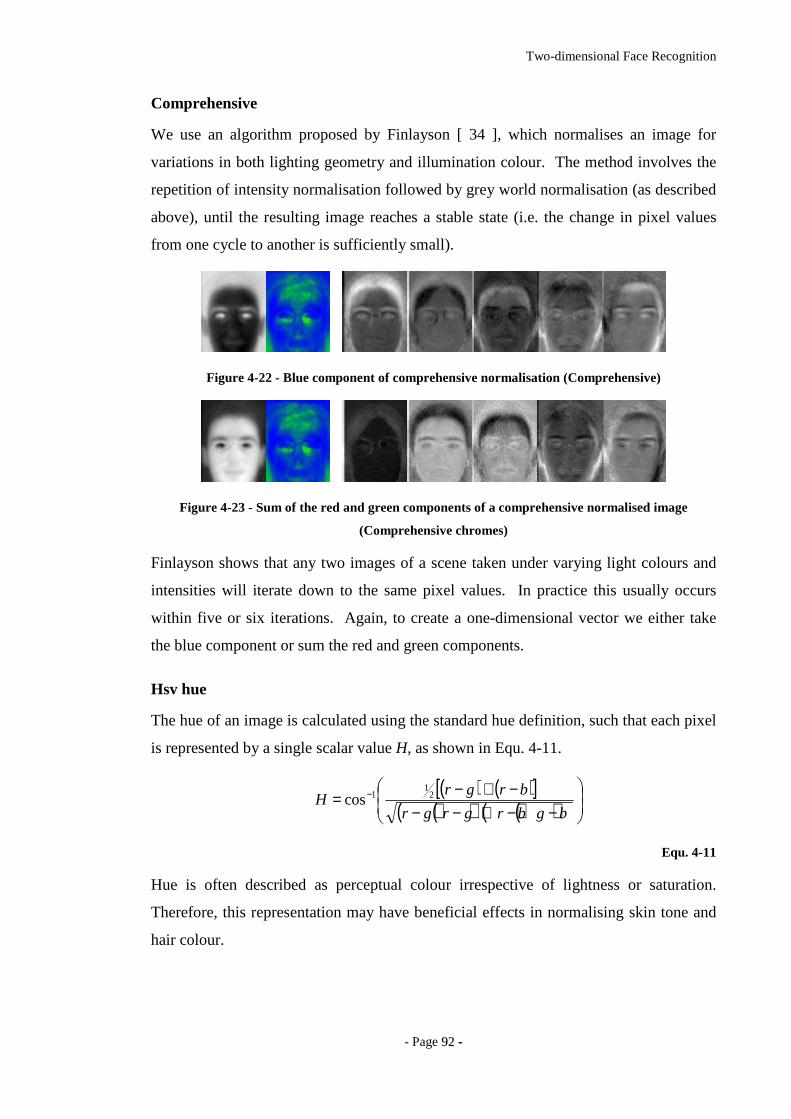
Two-dimensional Face Recognition
- Page 9922 --
Comprehensive
We use an algorithm proposed by Finlayson [ 34 ], which normalises an image for
variations in both lighting geometry and illumination colour. The method involves the
repetition of intensity normalisation followed by grey world normalisation (as described
above), until the resulting image reaches a stable state (i.e. the change in pixel values
from one cycle to another is sufficiently small).
Figure 4-22 - Blue component of comprehensive normalisation (Comprehensive)
Figure 4-23 - Sum of the red and green components of a comprehensive normalised image
(Comprehensive chromes)
Finlayson shows that any two images of a scene taken under varying light colours and
intensities will iterate down to the same pixel values. In practice this usually occurs
within five or six iterations. Again, to create a one-dimensional vector we either take
the blue component or sum the red and green components.
Hsv hue
The hue of an image is calculated using the standard hue definition, such that each pixel
is represented by a single scalar value H, as shown in Equ. 4-11.
( ) ( )[ ]( )( ) ( )( )
−−+−−−+−= −
bgbrgrgr
brgrH 2
11cos
Equ. 4-11
Hue is often described as perceptual colour irrespective of lightness or saturation.
Therefore, this representation may have beneficial effects in normalising skin tone and
hair colour.
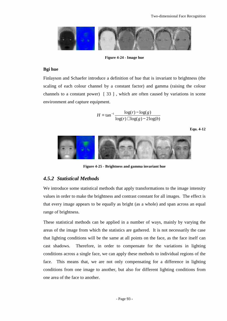
Two-dimensional Face Recognition
- Page 9933 --
Figure 4-24 - Image hue
Bgi hue
Finlayson and Schaefer introduce a definition of hue that is invariant to brightness (the
scaling of each colour channel by a constant factor) and gamma (raising the colour
channels to a constant power) [ 33 ] , which are often caused by variations in scene
environment and capture equipment.
)log(2)log()log(
)log()log(tan 1
bgr
grH
−+−= −
Equ. 4-12
Figure 4-25 - Brightness and gamma invariant hue
4.5.2 Statistical Methods
We introduce some statistical methods that apply transformations to the image intensity
values in order to make the brightness and contrast constant for all images. The effect is
that every image appears to be equally as bright (as a whole) and span across an equal
range of brightness.
These statistical methods can be applied in a number of ways, mainly by varying the
areas of the image from which the statistics are gathered. It is not necessarily the case
that lighting conditions will be the same at all points on the face, as the face itself can
cast shadows. Therefore, in order to compensate for the variations in lighting
conditions across a single face, we can apply these methods to individual regions of the
face. This means that, we are not only compensating for a difference in lighting
conditions from one image to another, but also for different lighting conditions from
one area of the face to another.
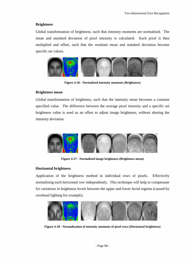
Two-dimensional Face Recognition
- Page 9944 --
Brightness
Global transformation of brightness, such that intensity moments are normalised. The
mean and standard deviation of pixel intensity is calculated. Each pixel is then
multiplied and offset, such that the resultant mean and standard deviation become
specific set values.
Figure 4-26 - Normalised intensity moments (Brightness)
Brightness mean
Global transformation of brightness, such that the intensity mean becomes a constant
specified value. The difference between the average pixel intensity and a specific set
brightness value is used as an offset to adjust image brightness, without altering the
intensity deviation.
Figure 4-27 - Normalised image brightness (Brightness mean)
Horizontal brightness
Application of the brightness method to individual rows of pixels. Effectively
normalising each horizontal row independently. This technique will help to compensate
for variations in brightness levels between the upper and lower facial regions (caused by
overhead lighting for example).
Figure 4-28 - Normalisation of intensity moments of pixel rows (Horizontal brightness)
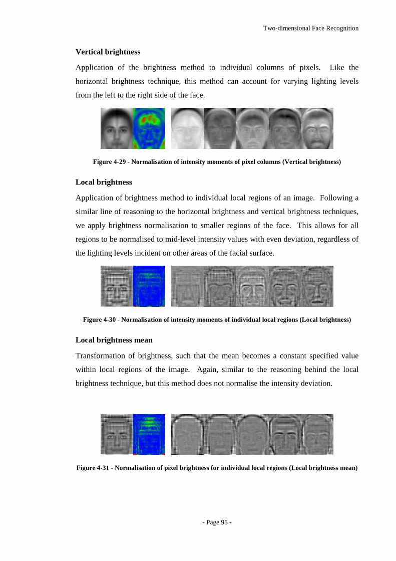
Two-dimensional Face Recognition
- Page 9955 --
Vertical brightness
Application of the brightness method to individual columns of pixels. Like the
horizontal brightness technique, this method can account for varying lighting levels
from the left to the right side of the face.
Figure 4-29 - Normalisation of intensity moments of pixel columns (Vertical brightness)
Local brightness
Application of brightness method to individual local regions of an image. Following a
similar line of reasoning to the horizontal brightness and vertical brightness techniques,
we apply brightness normalisation to smaller regions of the face. This allows for all
regions to be normalised to mid-level intensity values with even deviation, regardless of
the lighting levels incident on other areas of the facial surface.
Figure 4-30 - Normalisation of intensity moments of individual local regions (Local brightness)
Local brightness mean
Transformation of brightness, such that the mean becomes a constant specified value
within local regions of the image. Again, similar to the reasoning behind the local
brightness technique, but this method does not normalise the intensity deviation.
Figure 4-31 - Normalisation of pixel brightness for individual local regions (Local brightness mean)
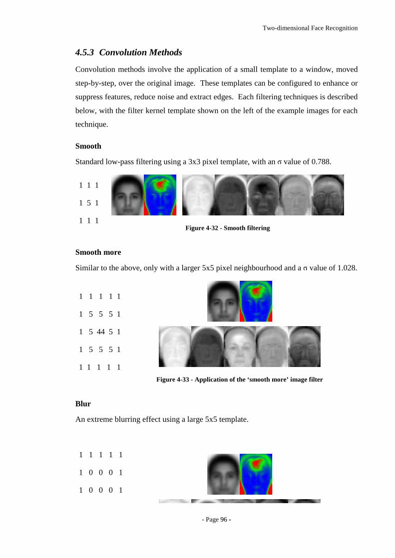
Two-dimensional Face Recognition
- Page 9966 --
4.5.3 Convolution Methods
Convolution methods involve the application of a small template to a window, moved
step-by-step, over the original image. These templates can be configured to enhance or
suppress features, reduce noise and extract edges. Each filtering techniques is described
below, with the filter kernel template shown on the left of the example images for each
technique.
Smooth
Standard low-pass filtering using a 3x3 pixel template, with an value of 0.788.
1 1 1
1 5 1
1 1 1
Figure 4-32 - Smooth filtering
Smooth more
Similar to the above, only with a larger 5x5 pixel neighbourhood and a value of 1.028.
1 1 1 1 1
1 5 5 5 1
1 5 44 5 1
1 5 5 5 1
1 1 1 1 1
Figure 4-33 - Application of the ‘smooth more’ image filter
Blur
An extreme blurring effect using a large 5x5 template.
1 1 1 1 1
1 0 0 0 1
1 0 0 0 1
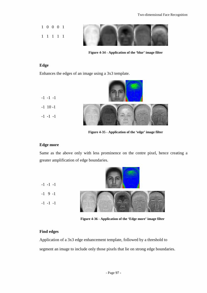
Two-dimensional Face Recognition
- Page 9977 --
1 0 0 0 1
1 1 1 1 1
Figure 4-34 - Application of the ‘blur’ image filter
Edge
Enhances the edges of an image using a 3x3 template.
-1 -1 -1
-1 10 -1
-1 -1 -1
Figure 4-35 - Application of the ‘edge’ image filter
Edge more
Same as the above only with less prominence on the centre pixel, hence creating a
greater amplification of edge boundaries.
-1 -1 -1
-1 9 -1
-1 -1 -1
Figure 4-36 - Application of the ‘Edge more’ image filter
Find edges
Application of a 3x3 edge enhancement template, followed by a threshold to
segment an image to include only those pixels that lie on strong edge boundaries.
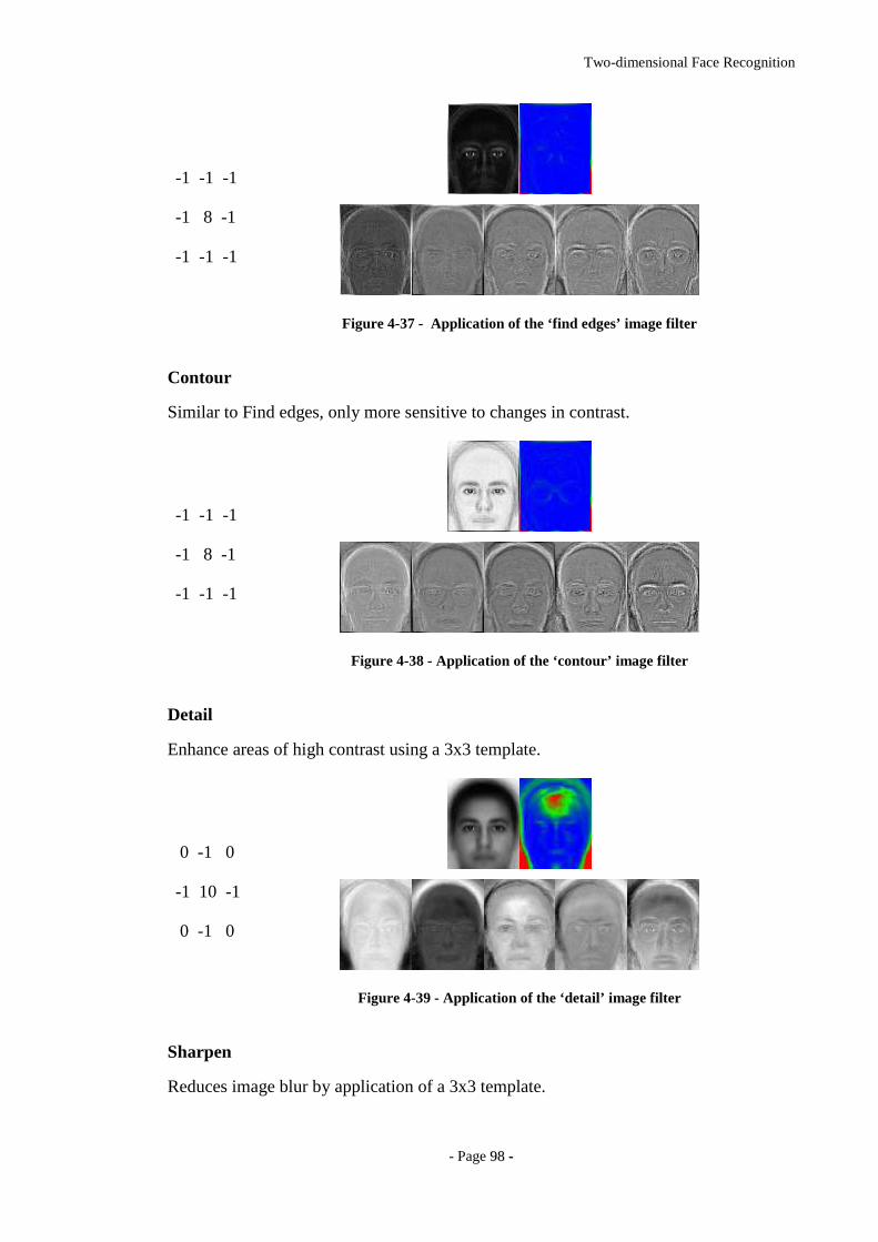
Two-dimensional Face Recognition
- Page 9988 --
-1 -1 -1
-1 8 -1
-1 -1 -1
Figure 4-37 - Application of the ‘find edges’ image filter
Contour
Similar to Find edges, only more sensitive to changes in contrast.
-1 -1 -1
-1 8 -1
-1 -1 -1
Figure 4-38 - Application of the ‘contour’ image filter
Detail
Enhance areas of high contrast using a 3x3 template.
0 -1 0
-1 10 -1
0 -1 0
Figure 4-39 - Application of the ‘detail’ image filter
Sharpen
Reduces image blur by application of a 3x3 template.
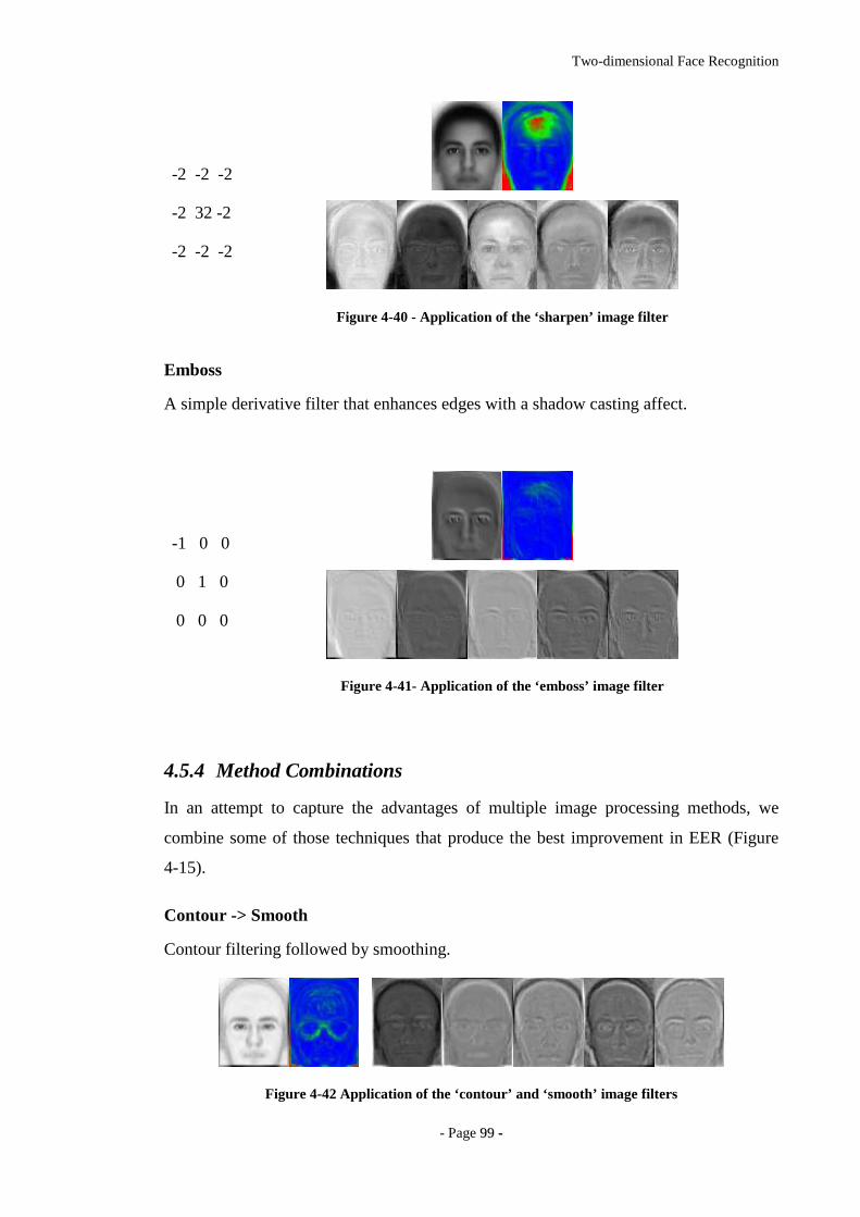
Two-dimensional Face Recognition
- Page 9999 --
-2 -2 -2
-2 32 -2
-2 -2 -2
Figure 4-40 - Application of the ‘sharpen’ image filter
Emboss
A simple derivative filter that enhances edges with a shadow casting affect.
-1 0 0
0 1 0
0 0 0
Figure 4-41- Application of the ‘emboss’ image filter
4.5.4 Method Combinations
In an attempt to capture the advantages of multiple image processing methods, we
combine some of those techniques that produce the best improvement in EER (Figure
4-15).
Contour -> Smooth
Contour filtering followed by smoothing.
Figure 4-42 Application of the ‘contour’ and ‘smooth’ image filters
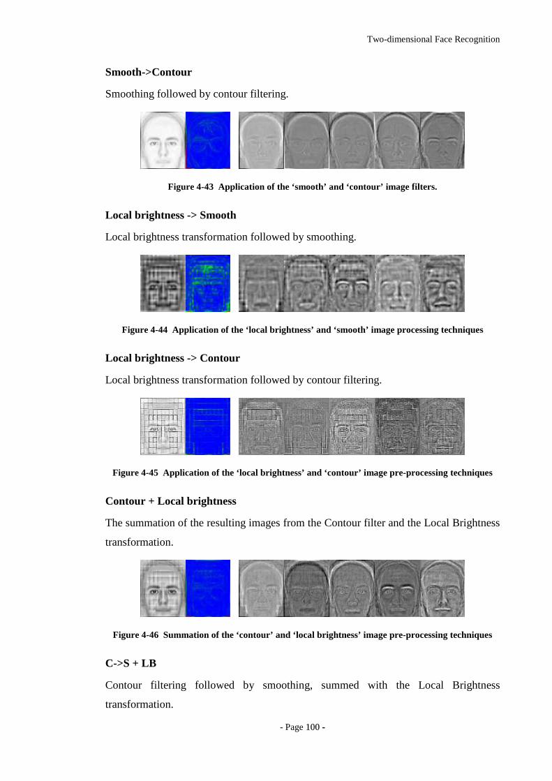
Two-dimensional Face Recognition
- Page 110000 --
Smooth->Contour
Smoothing followed by contour filtering.
Figure 4-43 Application of the ‘smooth’ and ‘contour’ image filters.
Local brightness -> Smooth
Local brightness transformation followed by smoothing.
Figure 4-44 Application of the ‘local brightness’ and ‘smooth’ image processing techniques
Local brightness -> Contour
Local brightness transformation followed by contour filtering.
Figure 4-45 Application of the ‘local brightness’ and ‘contour’ image pre-processing techniques
Contour + Local brightness
The summation of the resulting images from the Contour filter and the Local Brightness
transformation.
Figure 4-46 Summation of the ‘contour’ and ‘local brightness’ image pre-processing techniques
C->S + LB
Contour filtering followed by smoothing, summed with the Local Brightness
transformation.
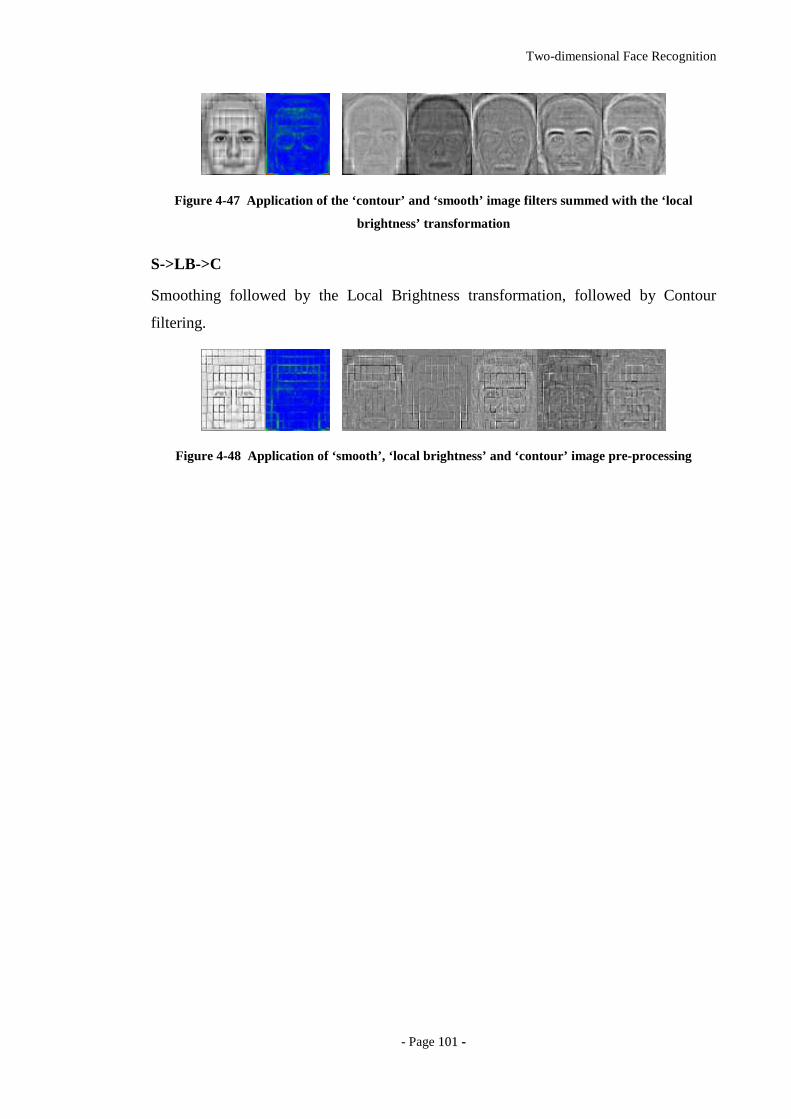
Two-dimensional Face Recognition
- Page 110011 --
Figure 4-47 Application of the ‘contour’ and ‘smooth’ image filters summed with the ‘local
brightness’ transformation
S->LB->C
Smoothing followed by the Local Brightness transformation, followed by Contour
filtering.
Figure 4-48 Application of ‘smooth’, ‘local brightness’ and ‘contour’ image pre-processing
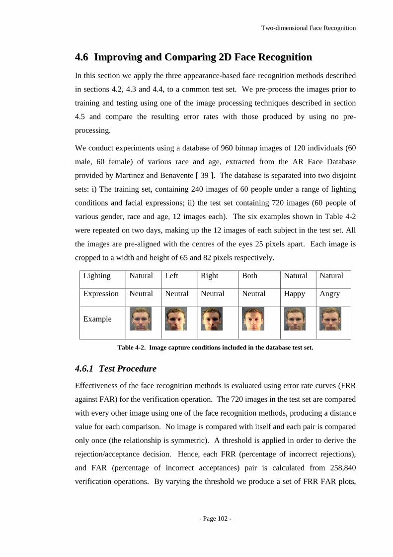
Two-dimensional Face Recognition
- Page 110022 --
44..66 II mmpprr oovviinngg aanndd CCoommppaarr iinngg 22DD FFaaccee RReeccooggnnii tt iioonn
In this section we apply the three appearance-based face recognition methods described
in sections 4.2, 4.3 and 4.4, to a common test set. We pre-process the images prior to
training and testing using one of the image processing techniques described in section
4.5 and compare the resulting error rates with those produced by using no pre-
processing.
We conduct experiments using a database of 960 bitmap images of 120 individuals (60
male, 60 female) of various race and age, extracted from the AR Face Database
provided by Martinez and Benavente [ 39 ]. The database is separated into two disjoint
sets: i) The training set, containing 240 images of 60 people under a range of lighting
conditions and facial expressions; ii) the test set containing 720 images (60 people of
various gender, race and age, 12 images each). The six examples shown in Table 4-2
were repeated on two days, making up the 12 images of each subject in the test set. All
the images are pre-aligned with the centres of the eyes 25 pixels apart. Each image is
cropped to a width and height of 65 and 82 pixels respectively.
Lighting Natural Left Right Both Natural Natural
Expression Neutral Neutral Neutral Neutral Happy Angry
Example
Table 4-2. Image capture conditions included in the database test set.
4.6.1 Test Procedure
Effectiveness of the face recognition methods is evaluated using error rate curves (FRR
against FAR) for the verification operation. The 720 images in the test set are compared
with every other image using one of the face recognition methods, producing a distance
value for each comparison. No image is compared with itself and each pair is compared
only once (the relationship is symmetric). A threshold is applied in order to derive the
rejection/acceptance decision. Hence, each FRR (percentage of incorrect rejections),
and FAR (percentage of incorrect acceptances) pair is calculated from 258,840
verification operations. By varying the threshold we produce a set of FRR FAR plots,
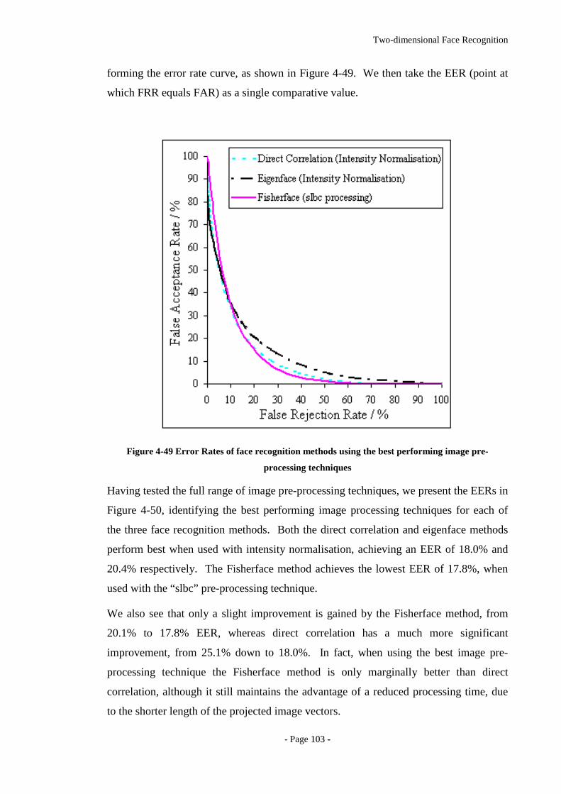
Two-dimensional Face Recognition
- Page 110033 --
forming the error rate curve, as shown in Figure 4-49. We then take the EER (point at
which FRR equals FAR) as a single comparative value.
Figure 4-49 Error Rates of face recognition methods using the best performing image pre-
processing techniques
Having tested the full range of image pre-processing techniques, we present the EERs in
Figure 4-50, identifying the best performing image processing techniques for each of
the three face recognition methods. Both the direct correlation and eigenface methods
perform best when used with intensity normalisation, achieving an EER of 18.0% and
20.4% respectively. The Fisherface method achieves the lowest EER of 17.8%, when
used with the “slbc” pre-processing technique.
We also see that only a slight improvement is gained by the Fisherface method, from
20.1% to 17.8% EER, whereas direct correlation has a much more significant
improvement, from 25.1% down to 18.0%. In fact, when using the best image pre-
processing technique the Fisherface method is only marginally better than direct
correlation, although it still maintains the advantage of a reduced processing time, due
to the shorter length of the projected image vectors.
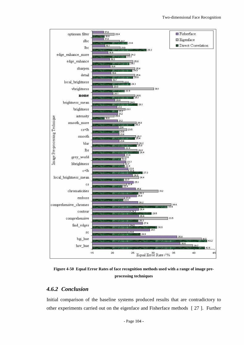
Two-dimensional Face Recognition
- Page 110044 --
Figure 4-50 Equal Error Rates of face recognition methods used with a range of image pre-
processing techniques
4.6.2 Conclusion
Initial comparison of the baseline systems produced results that are contradictory to
other experiments carried out on the eigenface and Fisherface methods [ 27 ]. Further

Two-dimensional Face Recognition
- Page 110055 --
investigation identified that the training set used for the Fisherface method did not
include sufficient examples of all conditions represented in the test data. In order for
the Fisherface method to perform recognition effectively, it is vital that the training set
is an adequate representation of the real application data. If such training data is not
available, or the real world image capture conditions cannot be predicted, the eigenface
and direct correlation methods are a better alternative. However, providing a suitable
training set is available, the Fisherface method has significantly lower error rates
(20.1%) than both the eigenface (25.5%) and direct correlation methods (25.1%), which
are comparable in terms of recognition accuracy.
Both methods have a space and time complexity of the same order, O(ni), where n is the
dimensionality of the face key data (or pixels in the image) and i the number of images
stored for comparison. However, with image vectors of 5330 elements (n), the
processing time and storage requirements of the direct correlation method are
significantly higher than the eigenface method, which uses vectors of only 59 elements.
Although the eigenface method has the additional training time of PCA, O(Mn2+n3),
where M is the number of items in the training set and n the dimensionality (pixels) of
the face images, the increased complexity at training is usually preferred over the
increased recognition time.
We have shown that the use of image pre-processing is able to significantly improve all
three methods of face recognition, reducing the EER of the eigenface, Fisherface and
direct correlation methods by 2.3, 5.1 and 7.1 percentage points respectively. However,
it has also become apparent that different image pre-processing techniques affect each
method of face recognition differently. Although some image processing techniques are
typically detrimental (blurring, smoothing, hue representations and comprehensive
normalisation) and others are generally beneficial (slbc, sharpen, detail, edge enhance)
to recognition, there are also techniques that will decrease error rates for some methods
while increasing error rates for others. The most prominent example of this is intensity
normalisation, which is evidently the best technique for both direct correlation and
eigenface methods, yet increases the EER for the Fisherface method.
This result suggests that although intensity normalisation is able to improve system
performance (supposedly by normalising lighting conditions), the LDA applied in the
Fisherface method is able to make better use of the non-normalised data. Therefore, it
must either be the case the intensity normalisation removes information that is useful for

Two-dimensional Face Recognition
- Page 110066 --
recognition (and utilised by the Fisherface method) or that the Fisherface method is able
to compensate for lighting variation more effectively than the intensity normalisation
algorithm.
Taking the best image pre-processing technique shows that the Fisherface method has
the lowest EER (17.8%), yet its lead over the other two methods is considerably
reduced. In this case, although much more computationally efficient, it is only
marginally better than direct correlation (EER 18.0%), but still maintains a significant
improvement over the eigenface method (EER 20.4%).
Further experimentation is required in order to identify which specific features are
enhanced by which pre-processing method and in what circumstances a given pre-
processing method is most effective. In addition, it may be the case that using a
different number of principal components will reduce error rates further, but this may
also be dependent on the pre-processing method used.
Three-Dimensional Face Recognition
- Page 110077 --
55 TThhrreeee--DDiimmeennssiioonnaall FFaaccee RReeccooggnnii tt iioonn
Despite significant advances in face recognition technology, it has yet to achieve the
levels of accuracy required for many commercial and industrial applications. This is
mainly due to the inaccuracies caused by the environmental circumstances under which
images are captured. Variation in lighting, facial expression and orientation all
significantly increase error rates, making it necessary to maintain consistent conditions
between query and gallery images for the system to function adequately. However, this
approach eliminates some of the key advantages offered by face recognition: a passive
biometric in the sense that it does not require subject co-operation.
The use of 3D face models is motivated by a number of factors. Firstly, by relying
purely on geometric shape, rather than colour and texture information, we render the
system invariant to lighting conditions. Secondly, the ability to rotate a facial structure
in 3D space, allowing for compensation of variations in pose, aids those methods
requiring alignment prior to recognition. Finally, the additional discriminatory depth
information in the facial surface structure, not available from two-dimensional images,
provides supplementary cues for recognition. As an example, eye separation can be
recovered from both sets of data, but nose depth can only easily be recovered from 3D
data. We do recognise however, that two-dimensional colour-texture information
provides a rich source of discriminatory information, which is forfeit if 3D data alone is
used. Therefore, the focus here is to first determine the ability of 3D data alone to form
the basis of a face recognition system, as compared to 2D systems. Additional research
can then identify methods of reintroducing normalised two-dimensional texture data in
order to reduce error rates further (see chapter 7.4).
We investigate the use of facial surface data, taken from 3D face models, as a substitute
for the more familiar two-dimensional images. In section 5.1 and 5.2 we discuss the 3D
face models used in systems development and how we achieve model alignment prior to
analysis and recognition. We then begin to explore 3D face recognition as we began
with 2D systems in section 4, using the simplest of recognition approaches: the direct
correlation method. In section 5.5 we continue the research pattern applied to 2D face
recognition, by taking the well-known eigenface method of face recognition, introduced
Three-Dimensional Face Recognition
- Page 110088 --
by Turk and Pentland [ 48 ] and adapt it for use on 3D data. Testing a range of surface
representations and distance metrics, we identify the most effective methods of
recognising faces using 3D surface structure. This experimentation is then extended to
use Linear Discriminant Analysis in section 5.6, before introducing a completely novel
approach (section 5.7), as a product of the experience gained from application of the
previous methodologies.
55..11 33DD FFaaccee MM ooddeellss
In order to evaluate and experiment with methods of 3D face recognition, we require a
large database of 3D face models. However, until recently, 3D capture methods have
been slow and cumbersome, requiring the subject to remain perfectly still. For these
reasons, 3D face recognition has remained relatively unexplored, when compared to the
wealth of research focusing on two-dimensional face recognition. Although some
investigations have experimented with 3D data, [ 3 ] [ 4 ][ 5 ][ 6 ][ 7 ][ 8 ] they have
had to rely on small test sets of 3D face models or used generic face models to enhance
two-dimensional images prior to recognition [ 9 ][ 10 ][ 11 ]. However, this research
demonstrates that the use of 3D information has the potential to improve face
recognition well beyond the current state of the art. With the emergence of new 3D
capture equipment, the population of a large 3D face database has now become viable.
Therefore, we have undertaken a project at The University of York to provide a database
of over five thousand 3D face models to facilitate research into 3D face recognition
technology [ 50 ]. The following section contains extracts from the requirement
specification used for acquisition of the 3D face database.
5.1.1 Data Acquisition
In this section we discuss the specifications of a database of 3D face models, intended
for use by Cybula Ltd, The University of York Computer Science, Electronics and
Psychology Departments. The University of York 3D Face Database (UOY3DFD) will
be used to facilitate research into such fields as automated face recognition, facial image
encoding and human facial perception. All data collected will be owned and managed
by Cybula Ltd. and made freely available to the other participants (mentioned above) for
academic research. It is intended that other researchers and companies will also be
granted access to the data for free or otherwise, if agreed by Cybula Ltd.

Three-Dimensional Face Recognition
- Page 110099 --
Multiple 3D models of each person are captured and stored in the Wavefront OBJ file
format [ 63 ] while corresponding texture images are stored in the bitmap file format.
The database is separated into two disjoint subsets:
• Set A is included to provide fast and efficient database population,
incorporating only the 15 most desired capture conditions.
• Set B is intended to provide some flexibility to the data acquisition
procedure. It has the option of containing a fewer or greater number of
models per person. This allows for more in-depth investigations or
capture sessions that may arise at exhibitions and conferences, where we
would be unable to capture all the models required in Set A, but could
take the opportunity to capture just a couple of models per person.
Software was written to facilitate a highly automated acquisition procedure for data Set
A. This software provides an electronic form to be filled out prior to each subject model
set acquisition. The information gathered is stored in a text file alongside each 3D
model and corresponding texture image. Face models are captured in a specific order
(following a predetermined script of capture conditions), as prompted by the acquisition
software. A consent agreement form was signed by each subject, prior to any image
acquisition. Files are automatically named and stored according to the criteria described
in Appendix I and II. The following information is stored about each subject:
• Gender
• Ethnicity
• Date of birth
• Age
• External features present
• Whether or not permission has been given by the subject to reproduce
their image in publications.
5.1.2 Capture Conditions
The database represents a range of age, gender, race and external features under a range
of controlled capture conditions, accepting the following limitations:
Three-Dimensional Face Recognition
- Page 111100 --
• The majority of subjects will be within the 18 to 60 years age range.
• We aim for an equal number of male and female subjects, although in the
interest of data quantity, some majority will be acceptable.
• For diversity of race we will initially rely on the diversity of the natural
population. However, should it be decided that a suitable representation
has not been obtained additional capture sessions will be undertaken.
• To capture 3D models of subjects with beards, glasses and other external
features, we will rely on the diversity of natural population and presence
of these features will be recorded in the database.
• No effort will be made to control lighting conditions other than ensuring
that lighting levels are within the operating capabilities of the 3D camera.
In order to generate face models at various head orientations, subjects were asked to
face reference points positioned roughly 45° above, below, to the left and right of the
camera, but no effort was made to enforce a precise angle of orientation.
Data Set A
Standard data set. Specified to encourage consistency of useful capture conditions.
Limited number of conditions to reduce capture time and increase throughput.
ID Description
01 Front facing, neutral expression, optimum distance from camera (1.7m
from unit to nose tip)
02 Neutral expression, (whole body) facing roughly 45 degrees left
03 Neutral expression, (whole body) left side profile (90 degrees left)
04 Neutral expression, (whole body) facing roughly 45 degrees right.
05 Neutral expression, (whole body) right side profile (90 degrees right)
06 Neutral expression, facing roughly 45 degrees up.
07 Neutral expression, facing roughly 45 degrees down.
08 Front facing, smiling.

Three-Dimensional Face Recognition
- Page 111111 --
09 Front facing, eyes closed.
10 Front facing, angry expression.
11 Front facing, neutral expression.
12 Front facing, eyebrows raised.
13 Front facing, mouth slightly parted.
14 Front facing, neutral expression, no glasses.
15 Front facing, neutral expression, no glasses, further away from the
camera (1.9m from unit to nose tip).
Table 5-1 All image capture conditions included in the UOY 3D Face Database.
Data Set B
Flexible data set. Specified to allow a broader range of capture conditions or data
acquisition sessions with very limited time and resources.
Set B is comprised of any conditions described in Set A. At least two models of each
person must be captured, but there is no limit on the maximum number of models per
person. In addition to the conditions described in Set A, additional conditions may be
included, in which case the condition details are recorded.
Table 5-2 Definition of data set B of the UOY 3D Face Database.
5.1.3 3D Face Data
In this section we now discuss the nature of the 3D face models being used in these
experiments. We describe the 3D-face model structure, multiple representations and
limitations in terms of resolution, noise and precision.
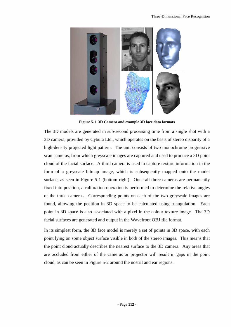
Three-Dimensional Face Recognition
- Page 111122 --
Figure 5-1 3D Camera and example 3D face data formats
The 3D models are generated in sub-second processing time from a single shot with a
3D camera, provided by Cybula Ltd., which operates on the basis of stereo disparity of a
high-density projected light pattern. The unit consists of two monochrome progressive
scan cameras, from which greyscale images are captured and used to produce a 3D point
cloud of the facial surface. A third camera is used to capture texture information in the
form of a greyscale bitmap image, which is subsequently mapped onto the model
surface, as seen in Figure 5-1 (bottom right). Once all three cameras are permanently
fixed into position, a calibration operation is performed to determine the relative angles
of the three cameras. Corresponding points on each of the two greyscale images are
found, allowing the position in 3D space to be calculated using triangulation. Each
point in 3D space is also associated with a pixel in the colour texture image. The 3D
facial surfaces are generated and output in the Wavefront OBJ file format.
In its simplest form, the 3D face model is merely a set of points in 3D space, with each
point lying on some object surface visible in both of the stereo images. This means that
the point cloud actually describes the nearest surface to the 3D camera. Any areas that
are occluded from either of the cameras or projector will result in gaps in the point
cloud, as can be seen in Figure 5-2 around the nostril and ear regions.
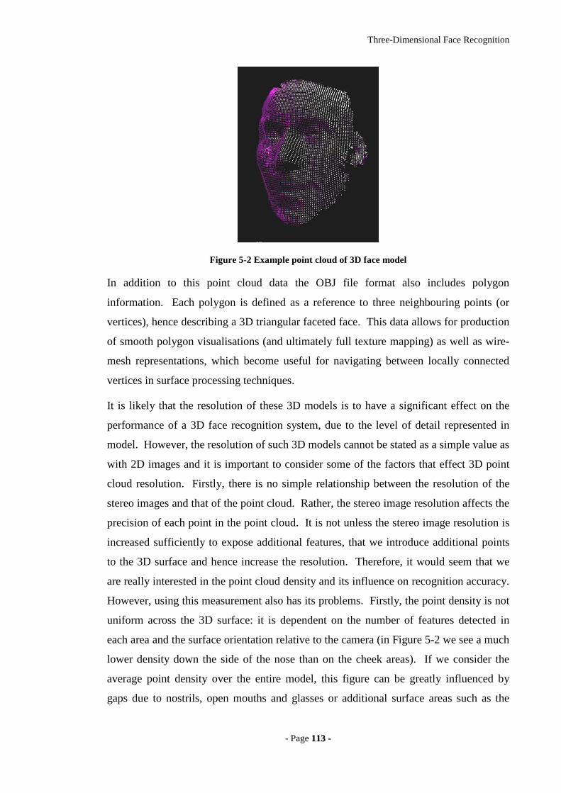
Three-Dimensional Face Recognition
- Page 111133 --
Figure 5-2 Example point cloud of 3D face model
In addition to this point cloud data the OBJ file format also includes polygon
information. Each polygon is defined as a reference to three neighbouring points (or
vertices), hence describing a 3D triangular faceted face. This data allows for production
of smooth polygon visualisations (and ultimately full texture mapping) as well as wire-
mesh representations, which become useful for navigating between locally connected
vertices in surface processing techniques.
It is likely that the resolution of these 3D models is to have a significant effect on the
performance of a 3D face recognition system, due to the level of detail represented in
model. However, the resolution of such 3D models cannot be stated as a simple value as
with 2D images and it is important to consider some of the factors that effect 3D point
cloud resolution. Firstly, there is no simple relationship between the resolution of the
stereo images and that of the point cloud. Rather, the stereo image resolution affects the
precision of each point in the point cloud. It is not unless the stereo image resolution is
increased sufficiently to expose additional features, that we introduce additional points
to the 3D surface and hence increase the resolution. Therefore, it would seem that we
are really interested in the point cloud density and its influence on recognition accuracy.
However, using this measurement also has its problems. Firstly, the point density is not
uniform across the 3D surface: it is dependent on the number of features detected in
each area and the surface orientation relative to the camera (in Figure 5-2 we see a much
lower density down the side of the nose than on the cheek areas). If we consider the
average point density over the entire model, this figure can be greatly influenced by
gaps due to nostrils, open mouths and glasses or additional surface areas such as the
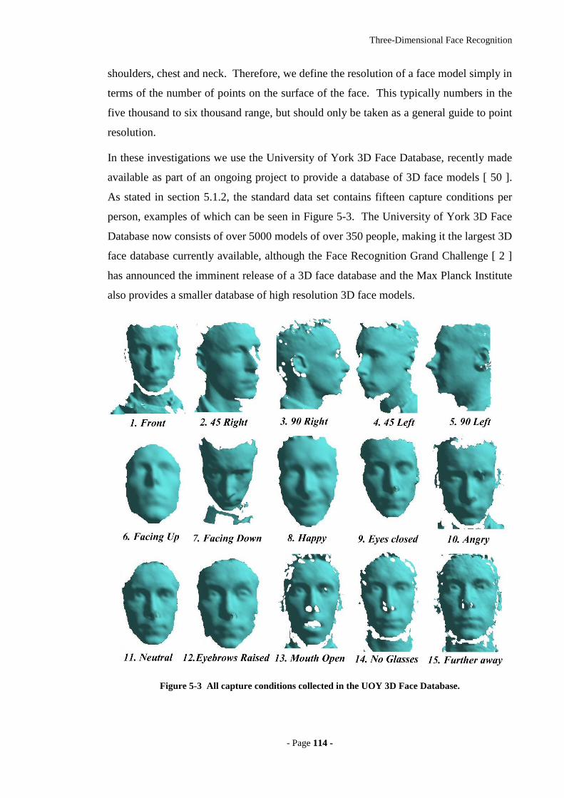
Three-Dimensional Face Recognition
- Page 111144 --
shoulders, chest and neck. Therefore, we define the resolution of a face model simply in
terms of the number of points on the surface of the face. This typically numbers in the
five thousand to six thousand range, but should only be taken as a general guide to point
resolution.
In these investigations we use the University of York 3D Face Database, recently made
available as part of an ongoing project to provide a database of 3D face models [ 50 ].
As stated in section 5.1.2, the standard data set contains fifteen capture conditions per
person, examples of which can be seen in Figure 5-3. The University of York 3D Face
Database now consists of over 5000 models of over 350 people, making it the largest 3D
face database currently available, although the Face Recognition Grand Challenge [ 2 ]
has announced the imminent release of a 3D face database and the Max Planck Institute
also provides a smaller database of high resolution 3D face models.
Figure 5-3 All capture conditions collected in the UOY 3D Face Database.

Three-Dimensional Face Recognition
- Page 111155 --
The research described in this thesis has been conducted as an ongoing series of sub-
projects running alongside the data collection efforts for the University of York 3D Face
Database. Because of this parallel progress, not all of the face data was available at the
beginning of the research and therefore different training and test sets have been used in
some of the experimentation. In particular, the earlier experiments were conducted
using a smaller test set. Although these experiments can be compared on a qualitative
basis, it does not provide the direct comparison necessary for a rigorous quantitative
scientific evaluation. Therefore, we address this issue in chapter 8, by performing a
final evaluation which compares the face recognition systems when applied to a
consistent set of test data.
55..22 OOrr iieennttaatt iioonn NNoorr mmaall iissaatt iioonn
As discussed earlier, 3D face recognition has the potential to compensate for variations
in head orientation from one face model acquisition to another. Unlike 2D images, 3D
face models can be rotated in 3D space, such that two facial surfaces become aligned
prior to recognition. Just as a 2D face recognition system could be made invariant to
scale and rotation around the z-axis by aligning two points on the face image, a 3D
system becomes invariant to scale and all directions of rotation by aligning three points
on the facial surface. However, for this to be successful, we must be able to consistently
localise these three points regardless of the orientation of the face at the time of capture.
This has proven to be a particularly difficult task worthy of further study as a separate
project and therefore we do not concentrate on the development of this process in any
great detail, choosing to focus on the recognition algorithm applied post-alignment.
However, rather than ignore the topic completely, we have developed a reasonably
robust 3D face model alignment algorithm, which functions adequately, given the
following assumptions:
• The tip of the nose is visible.
• The nose tip is the most protruding object on the 3D surface.
• The face is within 45 degrees of a front facing pose.
We apply the 3D orientation normalisation algorithm in a similar manner to the 2D
image alignment used in 2D face recognition systems. After localising facial landmarks,
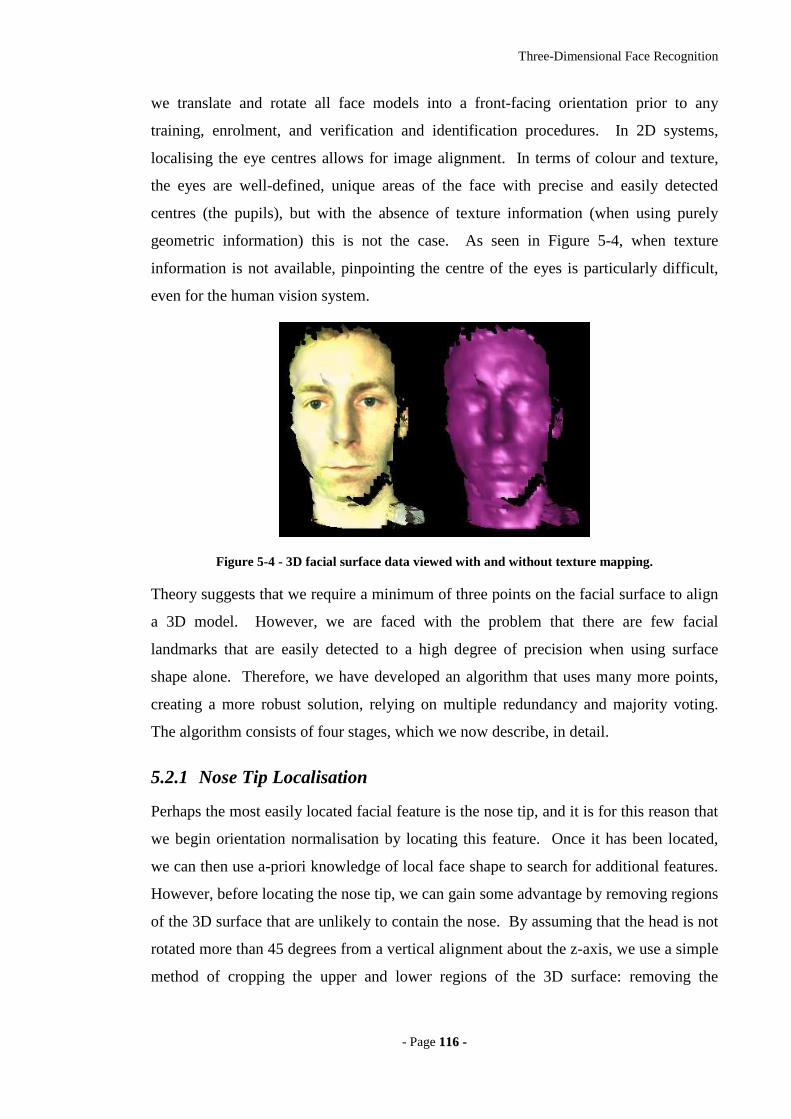
Three-Dimensional Face Recognition
- Page 111166 --
we translate and rotate all face models into a front-facing orientation prior to any
training, enrolment, and verification and identification procedures. In 2D systems,
localising the eye centres allows for image alignment. In terms of colour and texture,
the eyes are well-defined, unique areas of the face with precise and easily detected
centres (the pupils), but with the absence of texture information (when using purely
geometric information) this is not the case. As seen in Figure 5-4, when texture
information is not available, pinpointing the centre of the eyes is particularly difficult,
even for the human vision system.
Figure 5-4 - 3D facial surface data viewed with and without texture mapping.
Theory suggests that we require a minimum of three points on the facial surface to align
a 3D model. However, we are faced with the problem that there are few facial
landmarks that are easily detected to a high degree of precision when using surface
shape alone. Therefore, we have developed an algorithm that uses many more points,
creating a more robust solution, relying on multiple redundancy and majority voting.
The algorithm consists of four stages, which we now describe, in detail.
5.2.1 Nose Tip Localisation
Perhaps the most easily located facial feature is the nose tip, and it is for this reason that
we begin orientation normalisation by locating this feature. Once it has been located,
we can then use a-priori knowledge of local face shape to search for additional features.
However, before locating the nose tip, we can gain some advantage by removing regions
of the 3D surface that are unlikely to contain the nose. By assuming that the head is not
rotated more than 45 degrees from a vertical alignment about the z-axis, we use a simple
method of cropping the upper and lower regions of the 3D surface: removing the
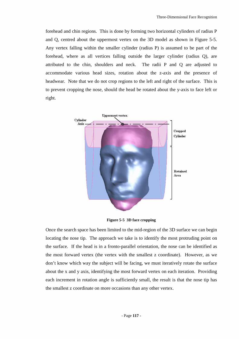
Three-Dimensional Face Recognition
- Page 111177 --
forehead and chin regions. This is done by forming two horizontal cylinders of radius P
and Q, centred about the uppermost vertex on the 3D model as shown in Figure 5-5.
Any vertex falling within the smaller cylinder (radius P) is assumed to be part of the
forehead, where as all vertices falling outside the larger cylinder (radius Q), are
attributed to the chin, shoulders and neck. The radii P and Q are adjusted to
accommodate various head sizes, rotation about the z-axis and the presence of
headwear. Note that we do not crop regions to the left and right of the surface. This is
to prevent cropping the nose, should the head be rotated about the y-axis to face left or
right.
Figure 5-5 3D face cropping
Once the search space has been limited to the mid-region of the 3D surface we can begin
locating the nose tip. The approach we take is to identify the most protruding point on
the surface. If the head is in a fronto-parallel orientation, the nose can be identified as
the most forward vertex (the vertex with the smallest z coordinate). However, as we
don’t know which way the subject will be facing, we must iteratively rotate the surface
about the x and y axis, identifying the most forward vertex on each iteration. Providing
each increment in rotation angle is sufficiently small, the result is that the nose tip has
the smallest z coordinate on more occasions than any other vertex.
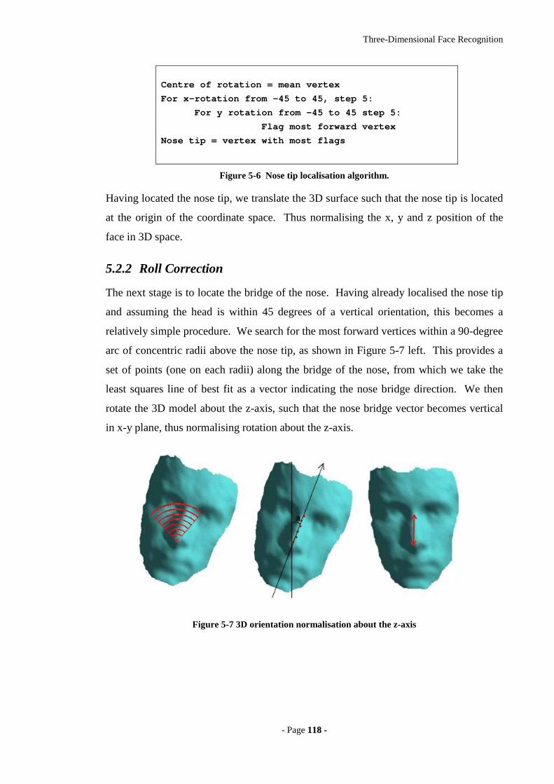
Three-Dimensional Face Recognition
- Page 111188 --
Centre of rotation = mean vertex
For x-rotation from –45 to 45, step 5:
For y rotation from –45 to 45 step 5:
Flag most forward vertex
Nose tip = vertex with most flags
Figure 5-6 Nose tip localisation algorithm.
Having located the nose tip, we translate the 3D surface such that the nose tip is located
at the origin of the coordinate space. Thus normalising the x, y and z position of the
face in 3D space.
5.2.2 Roll Correction
The next stage is to locate the bridge of the nose. Having already localised the nose tip
and assuming the head is within 45 degrees of a vertical orientation, this becomes a
relatively simple procedure. We search for the most forward vertices within a 90-degree
arc of concentric radii above the nose tip, as shown in Figure 5-7 left. This provides a
set of points (one on each radii) along the bridge of the nose, from which we take the
least squares line of best fit as a vector indicating the nose bridge direction. We then
rotate the 3D model about the z-axis, such that the nose bridge vector becomes vertical
in x-y plane, thus normalising rotation about the z-axis.
Figure 5-7 3D orientation normalisation about the z-axis
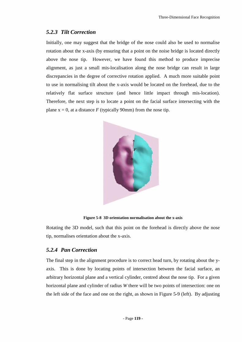
Three-Dimensional Face Recognition
- Page 111199 --
5.2.3 Tilt Correction
Initially, one may suggest that the bridge of the nose could also be used to normalise
rotation about the x-axis (by ensuring that a point on the noise bridge is located directly
above the nose tip. However, we have found this method to produce imprecise
alignment, as just a small mis-localisation along the nose bridge can result in large
discrepancies in the degree of corrective rotation applied. A much more suitable point
to use in normalising tilt about the x-axis would be located on the forehead, due to the
relatively flat surface structure (and hence little impact through mis-location).
Therefore, the next step is to locate a point on the facial surface intersecting with the
plane x = 0, at a distance F (typically 90mm) from the nose tip.
Figure 5-8 3D orientation normalisation about the x-axis
Rotating the 3D model, such that this point on the forehead is directly above the nose
tip, normalises orientation about the x-axis.
5.2.4 Pan Correction
The final step in the alignment procedure is to correct head turn, by rotating about the y-
axis. This is done by locating points of intersection between the facial surface, an
arbitrary horizontal plane and a vertical cylinder, centred about the nose tip. For a given
horizontal plane and cylinder of radius W there will be two points of intersection: one on
the left side of the face and one on the right, as shown in Figure 5-9 (left). By adjusting
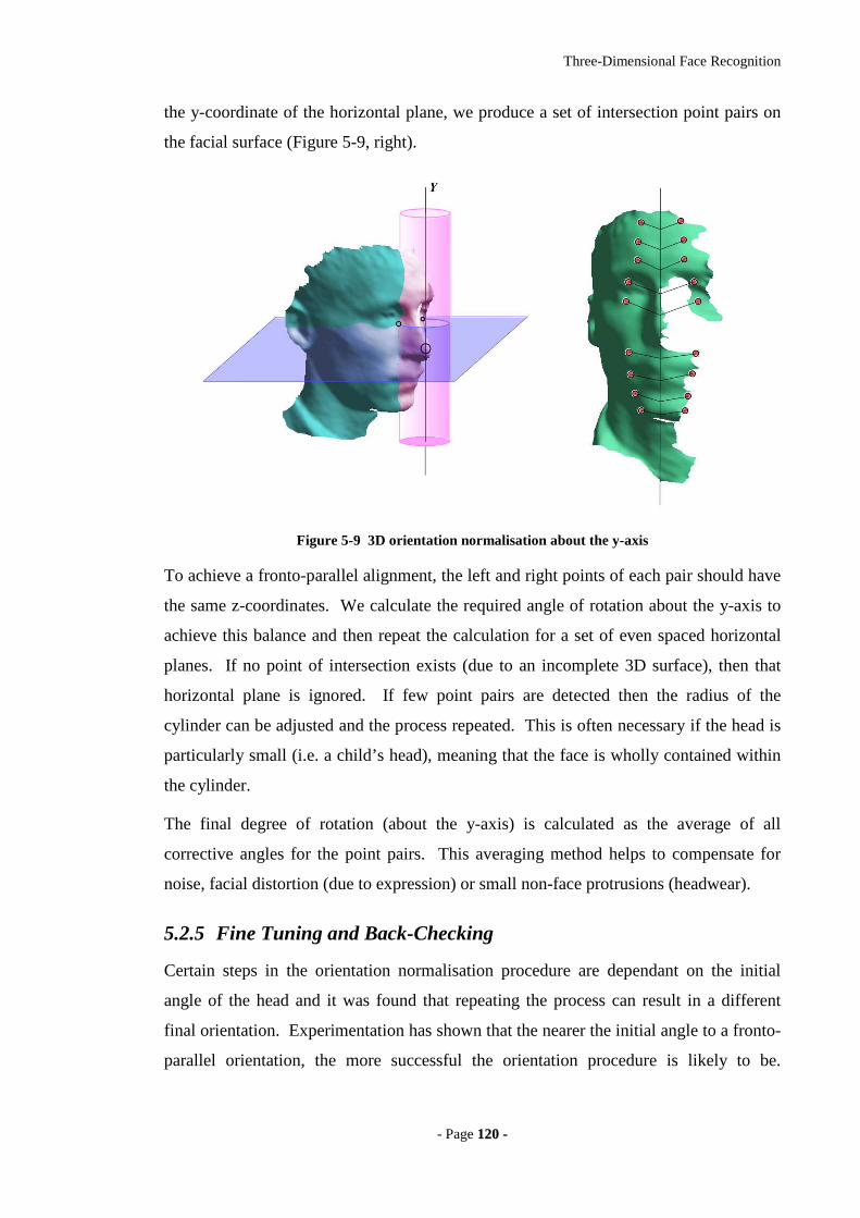
Three-Dimensional Face Recognition
- Page 112200 --
the y-coordinate of the horizontal plane, we produce a set of intersection point pairs on
the facial surface (Figure 5-9, right).
Figure 5-9 3D orientation normalisation about the y-axis
To achieve a fronto-parallel alignment, the left and right points of each pair should have
the same z-coordinates. We calculate the required angle of rotation about the y-axis to
achieve this balance and then repeat the calculation for a set of even spaced horizontal
planes. If no point of intersection exists (due to an incomplete 3D surface), then that
horizontal plane is ignored. If few point pairs are detected then the radius of the
cylinder can be adjusted and the process repeated. This is often necessary if the head is
particularly small (i.e. a child’s head), meaning that the face is wholly contained within
the cylinder.
The final degree of rotation (about the y-axis) is calculated as the average of all
corrective angles for the point pairs. This averaging method helps to compensate for
noise, facial distortion (due to expression) or small non-face protrusions (headwear).
5.2.5 Fine Tuning and Back-Checking
Certain steps in the orientation normalisation procedure are dependant on the initial
angle of the head and it was found that repeating the process can result in a different
final orientation. Experimentation has shown that the nearer the initial angle to a fronto-
parallel orientation, the more successful the orientation procedure is likely to be.

Three-Dimensional Face Recognition
- Page 112211 --
However, even if a successful alignment is not initially achieved, repeating the process
will usually improve the angle towards a more fronto-parallel orientation. This raises
the question of how to test for a correct alignment. Our chosen method is to compare
the depth map of an aligned 3D surface with the average face depth map. If the sum of
the square difference exceeds a given threshold, then the orientation normalisation
procedure can be repeated.
This method was chosen due to the quick and easy implementation and it is likely that
with a little more thought a much more robust method could be produced. One such
method could be to project the aligned face depth map into surface space (see section
4.1) and then compute the residual error, as described by Turk and Pentland [ 48 ]. This
would help with facial surfaces that may be substantially different from the average
face, yet still be face-shaped (and therefore represented in surface space). Another
orientation method may incorporate some of the IRAD techniques described in section
5.7, in which all three rotations are effectively detected simultaneously.

Three-Dimensional Face Recognition
- Page 112222 --
55..33 33DD SSuurr ffaaccee RReepprr eesseennttaatt iioonnss
In this section we describe the various representations of 3D surfaces used throughout
this thesis. We begin with a description of how depth maps are generated from the 3D
face models in section 5.3.1, before discussing the pre-processing techniques used to
generated other surface representations in section 5.3.2.
5.3.1 Depth Map Generation
3D surfaces can be stored in a variety of formats, including point clouds, meshes,
polygons, curve-splines etc., but it is the depth map representation that we choose as our
standard format for storage and processing. This is mainly due to its implementation as
a one-dimensional array, to which we can directly apply the direct correlation, PCA and
LDA algorithms used in the two-dimensional systems. Hence allowing a direct
comparison of the two approaches with little adaptation of the algorithms themselves.
In addition, the depth map representation can be conveniently stored as a greyscale
bitmap image, allowing for thumbnail browsing, cropping, scaling and filtering using
standard graphics packages and image processing libraries.
Prior to depth map generation it is often necessary to perform some form of smoothing
and noise reduction on the original 3D face model. A slight ripple effect is often
witnessed due to small inaccuracies in computation of point depth and areas of specula
reflection can result in spikes and pits. Such anomalies are easily removed using a two-
pass noise reduction procedure:
For each vertex in point cloud:
spike = maximum difference in depth to neighbour ing vertices
If absolute(spike) > N:
New vertex depth = average depth of neighbou ring vertices
For each vertex in point cloud:
New vertex depth = weighted average depth of nei ghbouring
vertices, where weighting is inversely proportio nal to
distance in the xy plane.
Figure 5-10 3D face model smoothing algorithm
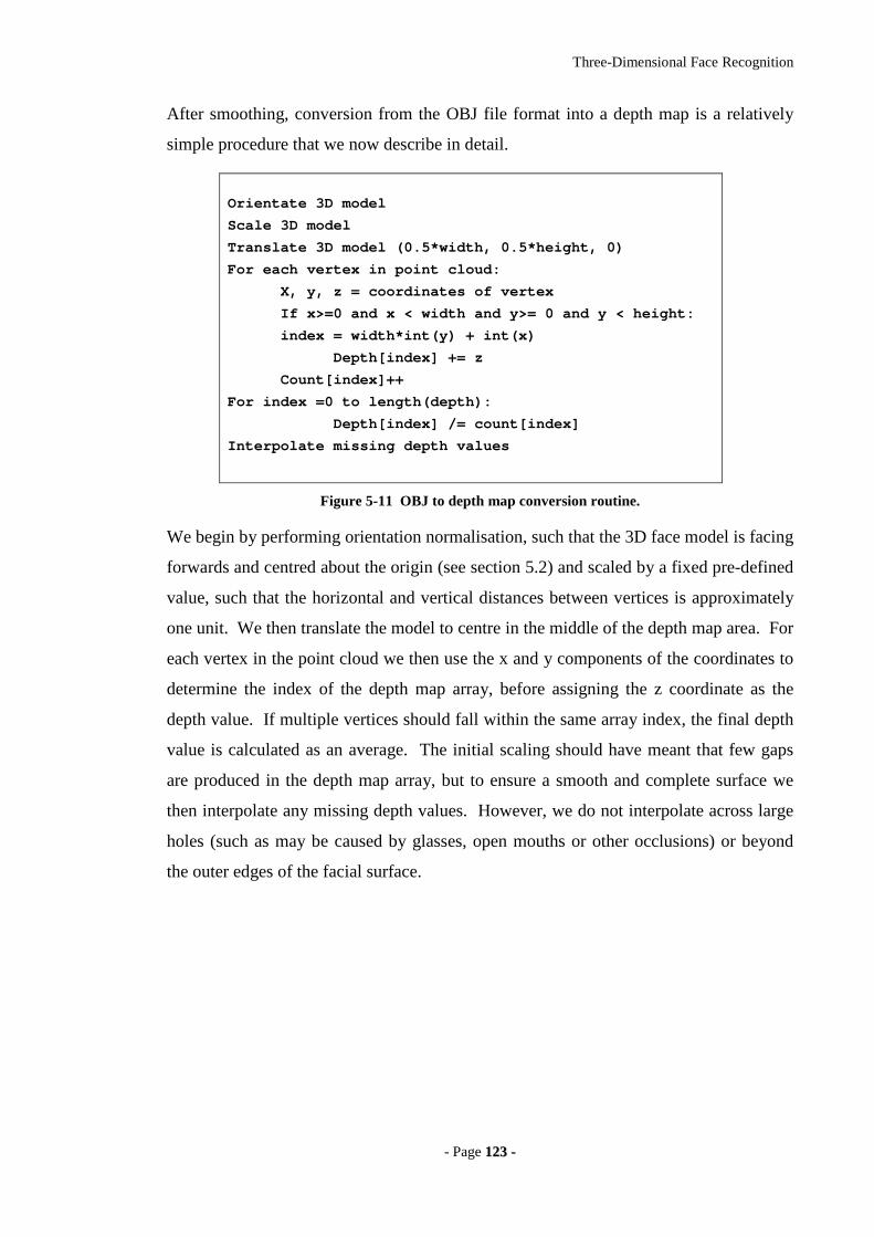
Three-Dimensional Face Recognition
- Page 112233 --
After smoothing, conversion from the OBJ file format into a depth map is a relatively
simple procedure that we now describe in detail.
Orientate 3D model
Scale 3D model
Translate 3D model (0.5*width, 0.5*height, 0)
For each vertex in point cloud:
X, y, z = coordinates of vertex
If x>=0 and x < width and y>= 0 and y < height:
index = width*int(y) + int(x)
Depth[index] += z
Count[index]++
For index =0 to length(depth):
Depth[index] /= count[index]
Interpolate missing depth values
Figure 5-11 OBJ to depth map conversion routine.
We begin by performing orientation normalisation, such that the 3D face model is facing
forwards and centred about the origin (see section 5.2) and scaled by a fixed pre-defined
value, such that the horizontal and vertical distances between vertices is approximately
one unit. We then translate the model to centre in the middle of the depth map area. For
each vertex in the point cloud we then use the x and y components of the coordinates to
determine the index of the depth map array, before assigning the z coordinate as the
depth value. If multiple vertices should fall within the same array index, the final depth
value is calculated as an average. The initial scaling should have meant that few gaps
are produced in the depth map array, but to ensure a smooth and complete surface we
then interpolate any missing depth values. However, we do not interpolate across large
holes (such as may be caused by glasses, open mouths or other occlusions) or beyond
the outer edges of the facial surface.
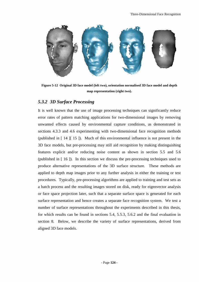
Three-Dimensional Face Recognition
- Page 112244 --
Figure 5-12 Original 3D face model (left two), orientation normalised 3D face model and depth
map representation (right two).
5.3.2 3D Surface Processing
It is well known that the use of image processing techniques can significantly reduce
error rates of pattern matching applications for two-dimensional images by removing
unwanted effects caused by environmental capture conditions, as demonstrated in
sections 4.3.3 and 4.6 experimenting with two-dimensional face recognition methods
(published in [ 14 ][ 15 ]). Much of this environmental influence is not present in the
3D face models, but pre-processing may still aid recognition by making distinguishing
features explicit and/or reducing noise content as shown in section 5.5 and 5.6
(published in [ 16 ]). In this section we discuss the pre-processing techniques used to
produce alternative representations of the 3D surface structure. These methods are
applied to depth map images prior to any further analysis in either the training or test
procedures. Typically, pre-processing algorithms are applied to training and test sets as
a batch process and the resulting images stored on disk, ready for eigenvector analysis
or face space projection later, such that a separate surface space is generated for each
surface representation and hence creates a separate face recognition system. We test a
number of surface representations throughout the experiments described in this thesis,
for which results can be found in sections 5.4, 5.5.3, 5.6.2 and the final evaluation in
section 8. Below, we describe the variety of surface representations, derived from
aligned 3D face models.
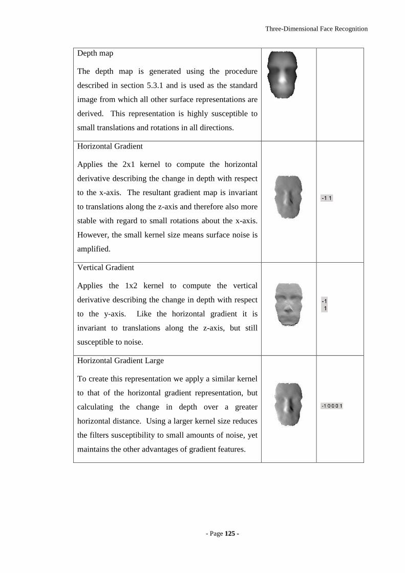
Three-Dimensional Face Recognition
- Page 112255 --
Depth map
The depth map is generated using the procedure
described in section 5.3.1 and is used as the standard
image from which all other surface representations are
derived. This representation is highly susceptible to
small translations and rotations in all directions.
Horizontal Gradient
Applies the 2x1 kernel to compute the horizontal
derivative describing the change in depth with respect
to the x-axis. The resultant gradient map is invariant
to translations along the z-axis and therefore also more
stable with regard to small rotations about the x-axis.
However, the small kernel size means surface noise is
amplified.
Vertical Gradient
Applies the 1x2 kernel to compute the vertical
derivative describing the change in depth with respect
to the y-axis. Like the horizontal gradient it is
invariant to translations along the z-axis, but still
susceptible to noise.
Horizontal Gradient Large
To create this representation we apply a similar kernel
to that of the horizontal gradient representation, but
calculating the change in depth over a greater
horizontal distance. Using a larger kernel size reduces
the filters susceptibility to small amounts of noise, yet
maintains the other advantages of gradient features.
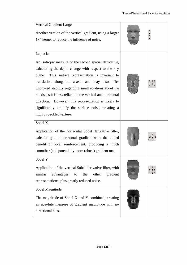
Three-Dimensional Face Recognition
- Page 112266 --
Vertical Gradient Large
Another version of the vertical gradient, using a larger
1x4 kernel to reduce the influence of noise.
Laplacian
An isotropic measure of the second spatial derivative,
calculating the depth change with respect to the x y
plane. This surface representation is invariant to
translation along the z-axis and may also offer
improved stability regarding small rotations about the
z-axis, as it is less reliant on the vertical and horizontal
direction. However, this representation is likely to
significantly amplify the surface noise, creating a
highly speckled texture.
Sobel X
Application of the horizontal Sobel derivative filter,
calculating the horizontal gradient with the added
benefit of local reinforcement, producing a much
smoother (and potentially more robust) gradient map.
Sobel Y
Application of the vertical Sobel derivative filter, with
similar advantages to the other gradient
representations, plus greatly reduced noise.
Sobel Magnitude
The magnitude of Sobel X and Y combined, creating
an absolute measure of gradient magnitude with no
directional bias.
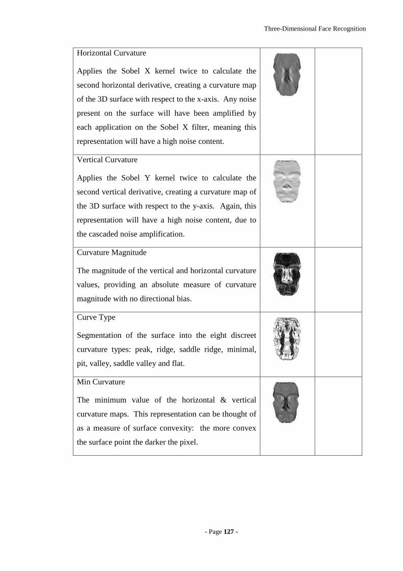
Three-Dimensional Face Recognition
- Page 112277 --
Horizontal Curvature
Applies the Sobel X kernel twice to calculate the
second horizontal derivative, creating a curvature map
of the 3D surface with respect to the x-axis. Any noise
present on the surface will have been amplified by
each application on the Sobel X filter, meaning this
representation will have a high noise content.
Vertical Curvature
Applies the Sobel Y kernel twice to calculate the
second vertical derivative, creating a curvature map of
the 3D surface with respect to the y-axis. Again, this
representation will have a high noise content, due to
the cascaded noise amplification.
Curvature Magnitude
The magnitude of the vertical and horizontal curvature
values, providing an absolute measure of curvature
magnitude with no directional bias.
Curve Type
Segmentation of the surface into the eight discreet
curvature types: peak, ridge, saddle ridge, minimal,
pit, valley, saddle valley and flat.
Min Curvature
The minimum value of the horizontal & vertical
curvature maps. This representation can be thought of
as a measure of surface convexity: the more convex
the surface point the darker the pixel.
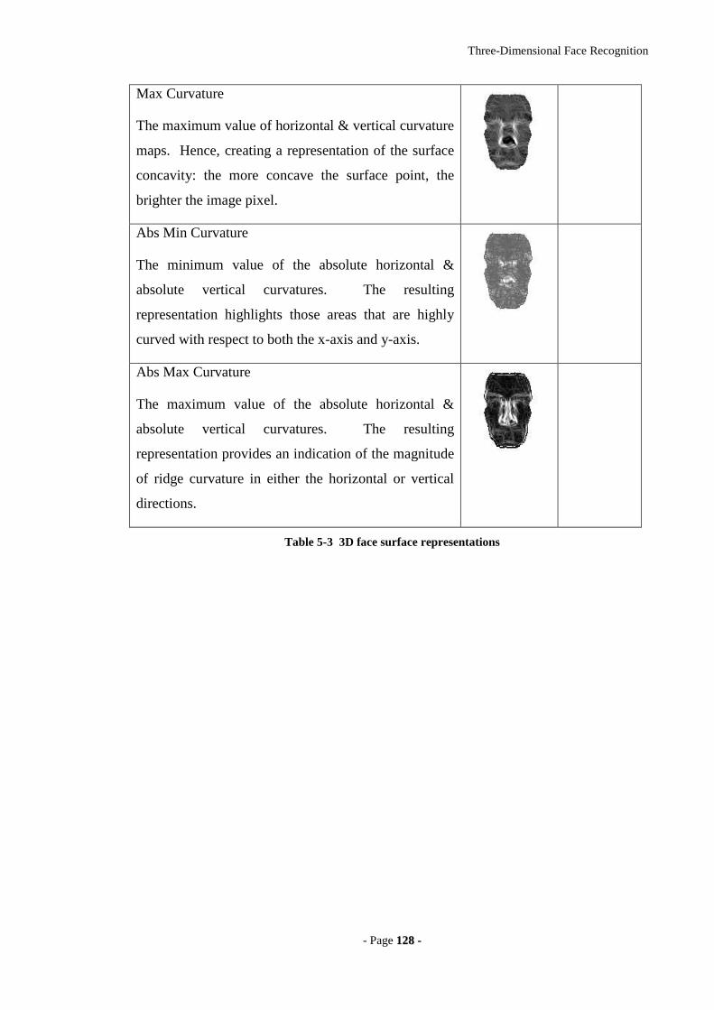
Three-Dimensional Face Recognition
- Page 112288 --
Max Curvature
The maximum value of horizontal & vertical curvature
maps. Hence, creating a representation of the surface
concavity: the more concave the surface point, the
brighter the image pixel.
Abs Min Curvature
The minimum value of the absolute horizontal &
absolute vertical curvatures. The resulting
representation highlights those areas that are highly
curved with respect to both the x-axis and y-axis.
Abs Max Curvature
The maximum value of the absolute horizontal &
absolute vertical curvatures. The resulting
representation provides an indication of the magnitude
of ridge curvature in either the horizontal or vertical
directions.
Table 5-3 3D face surface representations

Three-Dimensional Face Recognition
- Page 112299 --
55..44 DDii rr eecctt CCoorr rr eellaatt iioonn
The direct correlation approach is applied to 3D images (in the form of depth maps) as
for two-dimensional images: a simple direct comparison of the query and target images,
producing a difference value. However, in this case rather than using two-dimensional
intensity images of surface texture, we use 3D depth maps of the facial surface. Firstly,
3D face models are orientated to face directly forwards using our orientation
normalisation algorithm described in section 5.2, before being converted into a depth
map representation and compared using some distance metric and verified by
application of a threshold value. By altering this threshold value we are able to bias the
system towards either a low FAR (with a high FRR) or a low FRR (with a high FAR).
We experiment on a database of 290 depth maps, taken from the University of York 3D
Face Database, consisting of subjects of various race, age and gender with varying pose
and expression. No training set is required, as we do not perform any weighting or
image space analysis. Instead, this experimentation will provide an indication of the
effectiveness of a very rudimentary 3D face recognition system in its simplest form:
direction comparison of facial depth maps. We also demonstrate how various surface
representations result in different error rates, while referring the reading to section 5.3
for a detailed explanation of the various surface representations tested.
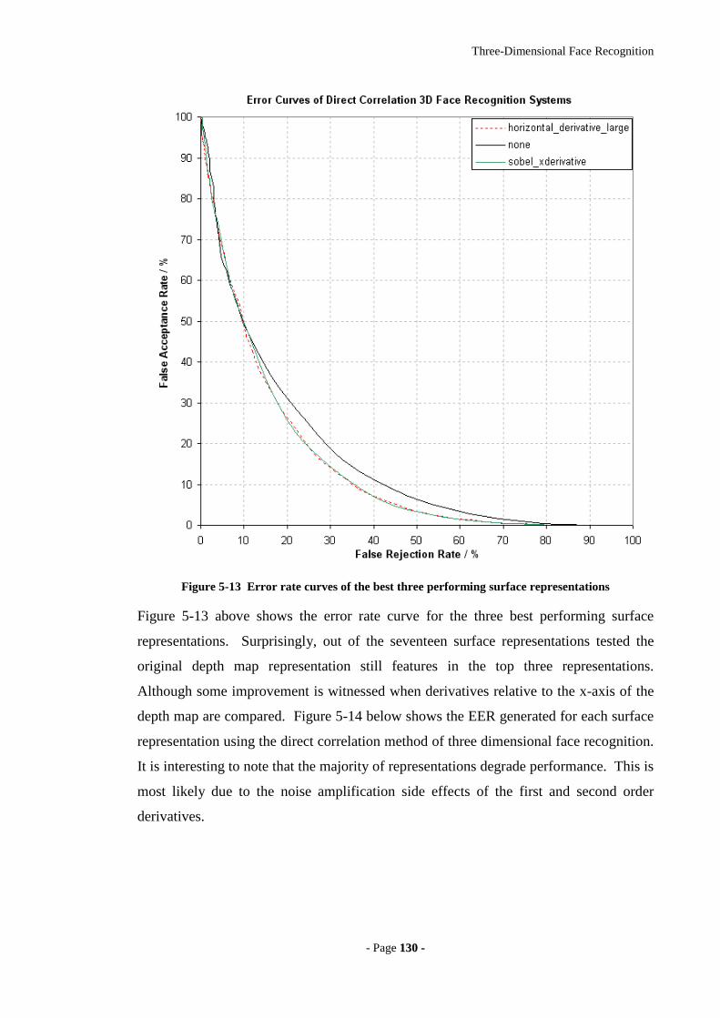
Three-Dimensional Face Recognition
- Page 113300 --
Figure 5-13 Error rate curves of the best three performing surface representations
Figure 5-13 above shows the error rate curve for the three best performing surface
representations. Surprisingly, out of the seventeen surface representations tested the
original depth map representation still features in the top three representations.
Although some improvement is witnessed when derivatives relative to the x-axis of the
depth map are compared. Figure 5-14 below shows the EER generated for each surface
representation using the direct correlation method of three dimensional face recognition.
It is interesting to note that the majority of representations degrade performance. This is
most likely due to the noise amplification side effects of the first and second order
derivatives.

Three-Dimensional Face Recognition
- Page 113311 --
Figure 5-14 Bar chart of the EER for each surface representation
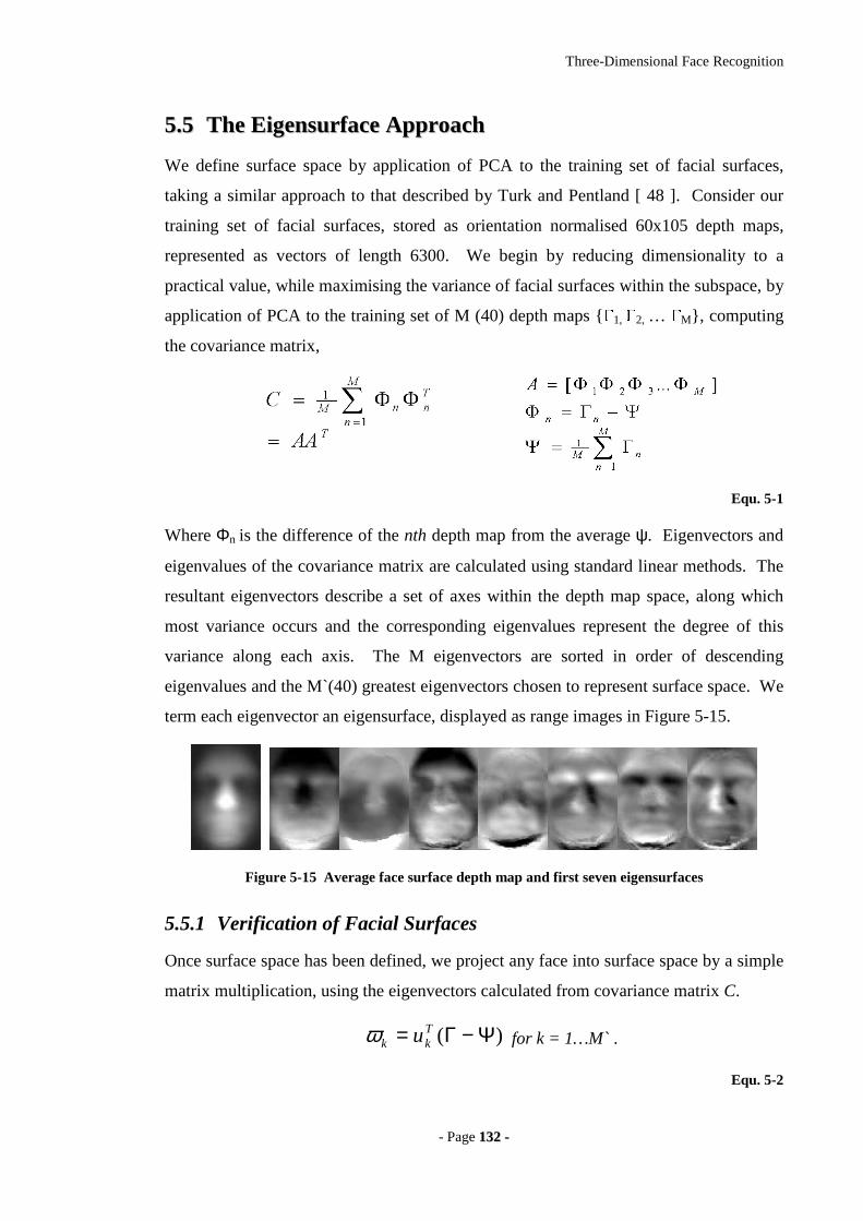
Three-Dimensional Face Recognition
- Page 113322 --
55..55 TThhee EEiiggeennssuurr ffaaccee AApppprr ooaacchh
We define surface space by application of PCA to the training set of facial surfaces,
taking a similar approach to that described by Turk and Pentland [ 48 ]. Consider our
training set of facial surfaces, stored as orientation normalised 60x105 depth maps,
represented as vectors of length 6300. We begin by reducing dimensionality to a
practical value, while maximising the variance of facial surfaces within the subspace, by
application of PCA to the training set of M (40) depth maps
1,
2, …
M, computing
the covariance matrix,
Equ. 5-1
Where Φn is the difference of the nth depth map from the average ψ. Eigenvectors and
eigenvalues of the covariance matrix are calculated using standard linear methods. The
resultant eigenvectors describe a set of axes within the depth map space, along which
most variance occurs and the corresponding eigenvalues represent the degree of this
variance along each axis. The M eigenvectors are sorted in order of descending
eigenvalues and the M`(40) greatest eigenvectors chosen to represent surface space. We
term each eigenvector an eigensurface, displayed as range images in Figure 5-15.
Figure 5-15 Average face surface depth map and first seven eigensurfaces
5.5.1 Verification of Facial Surfaces
Once surface space has been defined, we project any face into surface space by a simple
matrix multiplication, using the eigenvectors calculated from covariance matrix C.
)( Ψ−Γ= Tkk uω for k = 1…M .
Equ. 5-2
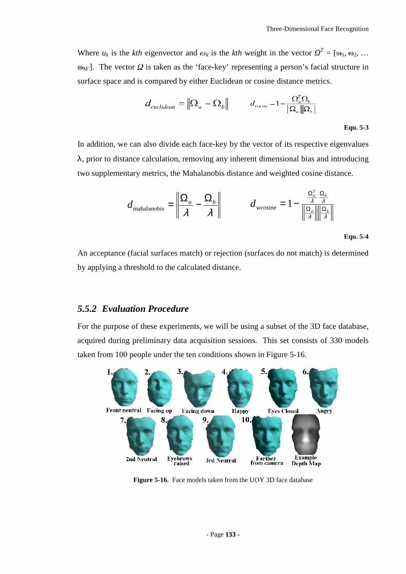
Three-Dimensional Face Recognition
- Page 113333 --
Where uk is the kth eigenvector and k is the kth weight in the vector T = [1, 2, … M`]. The vector
is taken as the ‘face-key’ representing a person’s facial structure in
surface space and is compared by either Euclidean or cosine distance metrics.
Equ. 5-3
In addition, we can also divide each face-key by the vector of its respective eigenvalues
λ, prior to distance calculation, removing any inherent dimensional bias and introducing
two supplementary metrics, the Mahalanobis distance and weighted cosine distance.
λλbad
Ω−Ω=smahalanobi λλ
λλba
bTa
d ΩΩ
ΩΩ
−= 1wcosine
Equ. 5-4
An acceptance (facial surfaces match) or rejection (surfaces do not match) is determined
by applying a threshold to the calculated distance.
5.5.2 Evaluation Procedure
For the purpose of these experiments, we will be using a subset of the 3D face database,
acquired during preliminary data acquisition sessions. This set consists of 330 models
taken from 100 people under the ten conditions shown in Figure 5-16.
Figure 5-16. Face models taken from the UOY 3D face database
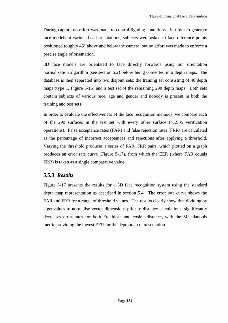
Three-Dimensional Face Recognition
- Page 113344 --
During capture no effort was made to control lighting conditions. In order to generate
face models at various head orientations, subjects were asked to face reference points
positioned roughly 45° above and below the camera, but no effort was made to enforce a
precise angle of orientation.
3D face models are orientated to face directly forwards using our orientation
normalisation algorithm (see section 5.2) before being converted into depth maps. The
database is then separated into two disjoint sets: the training set consisting of 40 depth
maps (type 1, Figure 5-16) and a test set of the remaining 290 depth maps. Both sets
contain subjects of various race, age and gender and nobody is present in both the
training and test sets.
In order to evaluate the effectiveness of the face recognition methods, we compare each
of the 290 surfaces in the test set with every other surface (41,905 verification
operations). False acceptance rates (FAR) and false rejection rates (FRR) are calculated
as the percentage of incorrect acceptances and rejections after applying a threshold.
Varying the threshold produces a series of FAR, FRR pairs, which plotted on a graph
produces an error rate curve (Figure 5-17), from which the EER (where FAR equals
FRR) is taken as a single comparative value.
5.5.3 Results
Figure 5-17 presents the results for a 3D face recognition system using the standard
depth map representation as described in section 5.4. The error rate curve shows the
FAR and FRR for a range of threshold values. The results clearly show that dividing by
eigenvalues to normalise vector dimensions prior to distance calculations, significantly
decreases error rates for both Euclidean and cosine distance, with the Mahalanobis
metric providing the lowest EER for the depth map representation.
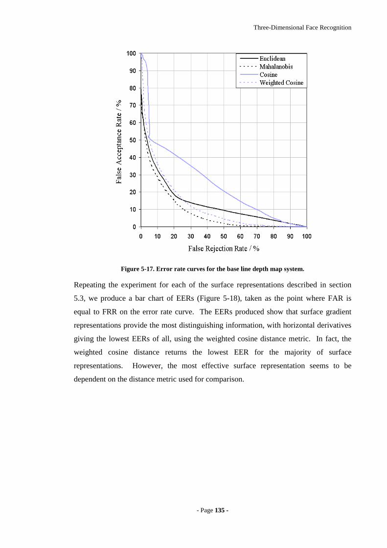
Three-Dimensional Face Recognition
- Page 113355 --
Figure 5-17. Error rate curves for the base line depth map system.
Repeating the experiment for each of the surface representations described in section
5.3, we produce a bar chart of EERs (Figure 5-18), taken as the point where FAR is
equal to FRR on the error rate curve. The EERs produced show that surface gradient
representations provide the most distinguishing information, with horizontal derivatives
giving the lowest EERs of all, using the weighted cosine distance metric. In fact, the
weighted cosine distance returns the lowest EER for the majority of surface
representations. However, the most effective surface representation seems to be
dependent on the distance metric used for comparison.
Three-Dimensional Face Recognition
- Page 113366 --
Figure 5-18. EERs of all 3D face recognition systems using a variety of surface representations and
distance metrics (right)
5.5.4 Conclusion
We have shown that a well-known two-dimensional face recognition method, namely
the eigenface method, can be adapted for use on 3D face models, which we name the
eigensurface method. Tests have been carried out on a large database of 3D facial
surfaces, captured under conditions that present typical difficulties when performing
recognition. The error rates produced from the 3D baseline system (19.1% EER using
Euclidean distance) are notably lower that those gathered in similar experiments using
two-dimensional images (25.5% EER) [ 15 ]. Although a more direct comparison is
required, using a common 2D/3D test database, in order to draw any quantitative
conclusions, initial results suggest that 3D face recognition has distinct advantages over
conventional two-dimensional approaches.
Experimenting with a number of surface representations, we have discovered that facial
surface gradient is more effective for recognition than depth and curvature
representations. In particular, horizontal gradients produce the lowest error rates,
seeming to indicate that horizontal derivatives provide more discriminatory information
than vertical. Another advantage is that gradients are likely to be more robust to
inaccuracies in the alignment procedure, as the derivatives will be invariant to
translations along the Z-axis.
Curvature representations do not seem to contain as much discriminatory information as
other surface representations. We find this surprising, as second derivatives should be
Three-Dimensional Face Recognition
- Page 113377 --
less sensitive to inaccuracies of orientation and translation along the Z-axis. However,
this could be a reflection of inadequate 3D model resolution and high noise content.
Testing four distance metrics has shown that the choice of method for face-key
comparisons has a considerable affect on resulting error rates. The Euclidean and cosine
metrics seem tailored to specific surface representations, suggesting that some create a
surface space in which between-class deviation is predominantly angular, whereas
others produce more radial deviation. It is also evident that dividing each face-key by
respective eigenvalues, normalising dimensional distribution, usually improves results
for both Euclidean and cosine distances. This indicates that the distribution along one
surface space dimension is not necessarily proportional to its discriminating ability and
that face-keys become more discriminative when all dimensions are weighted evenly.
However, this is not the case for some surface representations with higher EERs,
suggesting that these representations incorporate only a few dominant useful
components, which become masked when weighted evenly with the majority of less
discriminatory components.
Error rates of the best performing 3D eigensurface system (12.7% EER) are
substantially lower than the best two-dimensional systems (20.4% EER and 17.8%
EER) tested under similar circumstances in our previous investigations [ 14 ][ 15 ].
Although we recognise the differences between these experiments (most notably the
lack of a common 3D/2D test set), the results do show that geometric face structure is
useful for recognition when used independently from colour and texture and capable of
achieving high levels of accuracy. Given that the data capture method produces models
invariant to lighting conditions and provides the ability to recognise faces regardless of
pose, makes this system particularly attractive for use in security and surveillance
applications. However, more testing is required to identify the limitations of the
eigensurface method, although one obvious issue is the system’s reliance on accurate
orientation normalisation. Improved orientation normalisation techniques would likely
produce lower error rates or an alternative approach, in which an orientation invariant
representation was produced (removing the need to normalise orientation) may lead to
an improved recognition capability, as discussed in section 5.7.
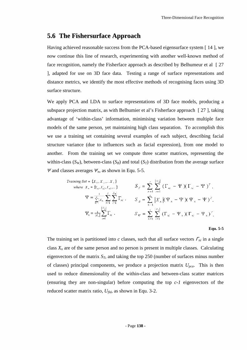
Three-Dimensional Face Recognition
- Page 113388 --
55..66 TThhee FFiisshheerr ssuurr ffaaccee AApppprr ooaacchh
Having achieved reasonable success from the PCA-based eigensurface system [ 14 ], we
now continue this line of research, experimenting with another well-known method of
face recognition, namely the Fisherface approach as described by Belhumeur et al [ 27
], adapted for use on 3D face data. Testing a range of surface representations and
distance metrics, we identify the most effective methods of recognising faces using 3D
surface structure.
We apply PCA and LDA to surface representations of 3D face models, producing a
subspace projection matrix, as with Belhumier et al’s Fisherface approach [ 27 ], taking
advantage of ‘within-class’ information, minimising variation between multiple face
models of the same person, yet maintaining high class separation. To accomplish this
we use a training set containing several examples of each subject, describing facial
structure variance (due to influences such as facial expression), from one model to
another. From the training set we compute three scatter matrices, representing the
within-class (SW), between-class (SB) and total (ST) distribution from the average surface and classes averages
n, as shown in Equ. 5-5.
Equ. 5-5
The training set is partitioned into c classes, such that all surface vectors Γni in a single
class Xn are of the same person and no person is present in multiple classes. Calculating
eigenvectors of the matrix ST, and taking the top 250 (number of surfaces minus number
of classes) principal components, we produce a projection matrix Upca. This is then
used to reduce dimensionality of the within-class and between-class scatter matrices
(ensuring they are non-singular) before computing the top c-1 eigenvectors of the
reduced scatter matrix ratio, Ufld, as shown in Equ. 3-2.
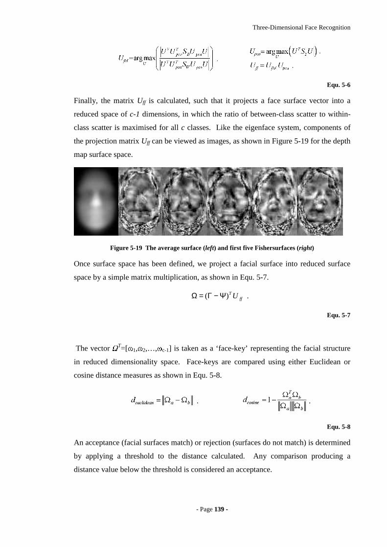
Three-Dimensional Face Recognition
- Page 113399 --
Equ. 5-6
Finally, the matrix Uff is calculated, such that it projects a face surface vector into a
reduced space of c-1 dimensions, in which the ratio of between-class scatter to within-
class scatter is maximised for all c classes. Like the eigenface system, components of
the projection matrix Uff can be viewed as images, as shown in Figure 5-19 for the depth
map surface space.
Figure 5-19 The average surface (left) and first five Fishersurfaces (right)
Once surface space has been defined, we project a facial surface into reduced surface
space by a simple matrix multiplication, as shown in Equ. 5-7.
ffTU)( Ψ−Γ=Ω .
Equ. 5-7
The vector T=[1,2,…,c-1] is taken as a ‘face-key’ representing the facial structure
in reduced dimensionality space. Face-keys are compared using either Euclidean or
cosine distance measures as shown in Equ. 5-8.
Equ. 5-8
An acceptance (facial surfaces match) or rejection (surfaces do not match) is determined
by applying a threshold to the distance calculated. Any comparison producing a
distance value below the threshold is considered an acceptance.
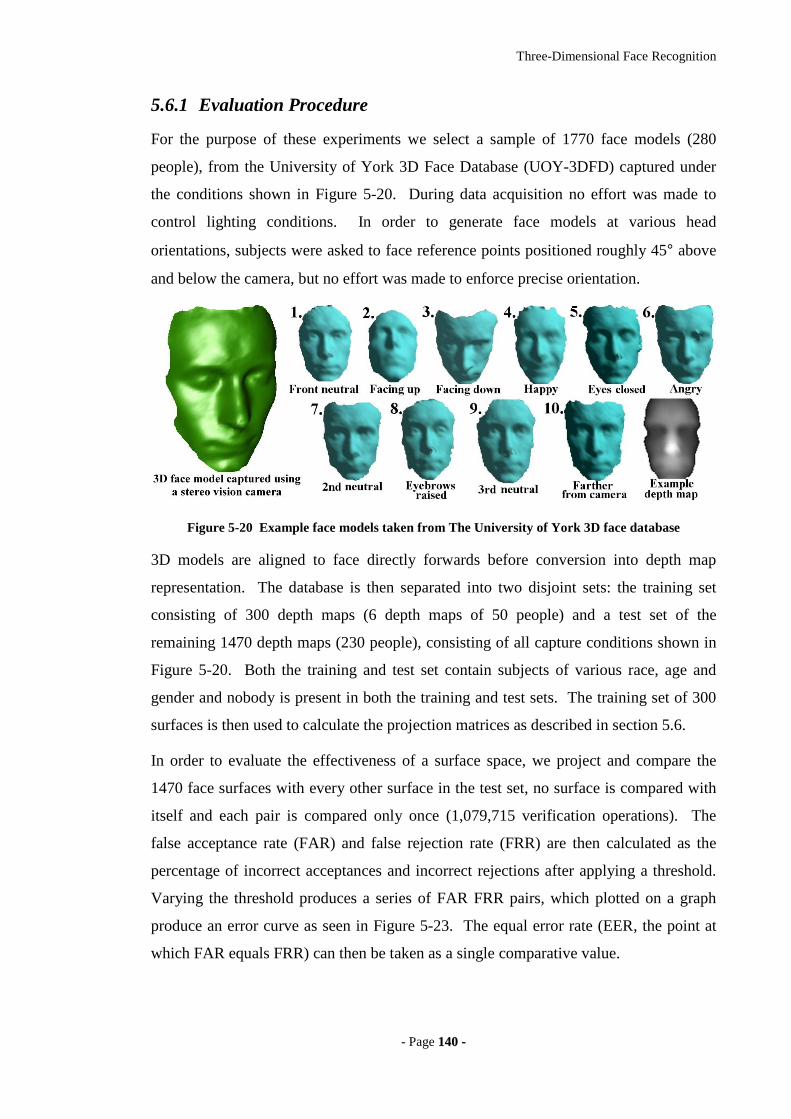
Three-Dimensional Face Recognition
- Page 114400 --
5.6.1 Evaluation Procedure
For the purpose of these experiments we select a sample of 1770 face models (280
people), from the University of York 3D Face Database (UOY-3DFD) captured under
the conditions shown in Figure 5-20. During data acquisition no effort was made to
control lighting conditions. In order to generate face models at various head
orientations, subjects were asked to face reference points positioned roughly 45° above
and below the camera, but no effort was made to enforce precise orientation.
Figure 5-20 Example face models taken from The University of York 3D face database
3D models are aligned to face directly forwards before conversion into depth map
representation. The database is then separated into two disjoint sets: the training set
consisting of 300 depth maps (6 depth maps of 50 people) and a test set of the
remaining 1470 depth maps (230 people), consisting of all capture conditions shown in
Figure 5-20. Both the training and test set contain subjects of various race, age and
gender and nobody is present in both the training and test sets. The training set of 300
surfaces is then used to calculate the projection matrices as described in section 5.6.
In order to evaluate the effectiveness of a surface space, we project and compare the
1470 face surfaces with every other surface in the test set, no surface is compared with
itself and each pair is compared only once (1,079,715 verification operations). The
false acceptance rate (FAR) and false rejection rate (FRR) are then calculated as the
percentage of incorrect acceptances and incorrect rejections after applying a threshold.
Varying the threshold produces a series of FAR FRR pairs, which plotted on a graph
produce an error curve as seen in Figure 5-23. The equal error rate (EER, the point at
which FAR equals FRR) can then be taken as a single comparative value.
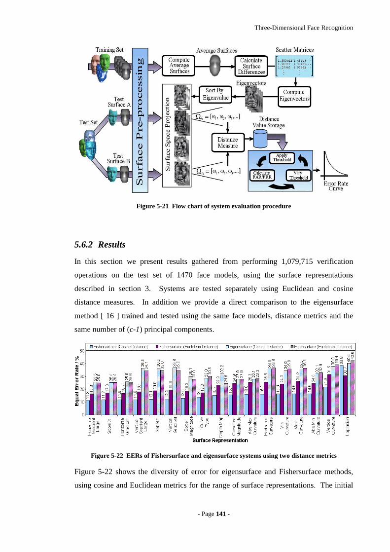
Three-Dimensional Face Recognition
- Page 114411 --
Figure 5-21 Flow chart of system evaluation procedure
5.6.2 Results
In this section we present results gathered from performing 1,079,715 verification
operations on the test set of 1470 face models, using the surface representations
described in section 3. Systems are tested separately using Euclidean and cosine
distance measures. In addition we provide a direct comparison to the eigensurface
method [ 16 ] trained and tested using the same face models, distance metrics and the
same number of (c-1) principal components.
Figure 5-22 EERs of Fishersurface and eigensurface systems using two distance metrics
Figure 5-22 shows the diversity of error for eigensurface and Fishersurface methods,
using cosine and Euclidean metrics for the range of surface representations. The initial
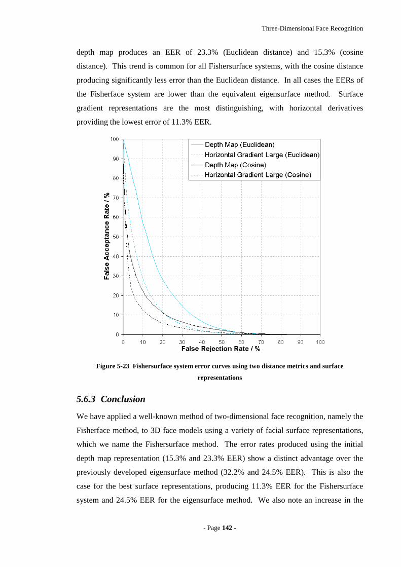
Three-Dimensional Face Recognition
- Page 114422 --
depth map produces an EER of 23.3% (Euclidean distance) and 15.3% (cosine
distance). This trend is common for all Fishersurface systems, with the cosine distance
producing significantly less error than the Euclidean distance. In all cases the EERs of
the Fisherface system are lower than the equivalent eigensurface method. Surface
gradient representations are the most distinguishing, with horizontal derivatives
providing the lowest error of 11.3% EER.
Figure 5-23 Fishersurface system error curves using two distance metrics and surface
representations
5.6.3 Conclusion
We have applied a well-known method of two-dimensional face recognition, namely the
Fisherface method, to 3D face models using a variety of facial surface representations,
which we name the Fishersurface method. The error rates produced using the initial
depth map representation (15.3% and 23.3% EER) show a distinct advantage over the
previously developed eigensurface method (32.2% and 24.5% EER). This is also the
case for the best surface representations, producing 11.3% EER for the Fishersurface
system and 24.5% EER for the eigensurface method. We also note an increase in the
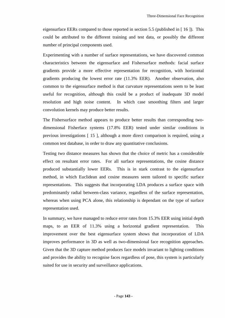
Three-Dimensional Face Recognition
- Page 114433 --
eigensurface EERs compared to those reported in section 5.5 (published in [ 16 ]). This
could be attributed to the different training and test data, or possibly the different
number of principal components used.
Experimenting with a number of surface representations, we have discovered common
characteristics between the eigensurface and Fishersurface methods: facial surface
gradients provide a more effective representation for recognition, with horizontal
gradients producing the lowest error rate (11.3% EER). Another observation, also
common to the eigensurface method is that curvature representations seem to be least
useful for recognition, although this could be a product of inadequate 3D model
resolution and high noise content. In which case smoothing filters and larger
convolution kernels may produce better results.
The Fishersurface method appears to produce better results than corresponding two-
dimensional Fisherface systems (17.8% EER) tested under similar conditions in
previous investigations [ 15 ], although a more direct comparison is required, using a
common test database, in order to draw any quantitative conclusions.
Testing two distance measures has shown that the choice of metric has a considerable
effect on resultant error rates. For all surface representations, the cosine distance
produced substantially lower EERs. This is in stark contrast to the eigensurface
method, in which Euclidean and cosine measures seem tailored to specific surface
representations. This suggests that incorporating LDA produces a surface space with
predominantly radial between-class variance, regardless of the surface representation,
whereas when using PCA alone, this relationship is dependant on the type of surface
representation used.
In summary, we have managed to reduce error rates from 15.3% EER using initial depth
maps, to an EER of 11.3% using a horizontal gradient representation. This
improvement over the best eigensurface system shows that incorporation of LDA
improves performance in 3D as well as two-dimensional face recognition approaches.
Given that the 3D capture method produces face models invariant to lighting conditions
and provides the ability to recognise faces regardless of pose, this system is particularly
suited for use in security and surveillance applications.

Three-Dimensional Face Recognition
- Page 114444 --
55..77 II RRAADD FFaaccee CCoonnttoouurr ss
In this section we propose a new technique for comparing 3D face models, which is
distinct from the appearance-based subspace methods discussed throughout the rest of
this thesis. This new approach is fuelled by our appreciation that subspace methods
require accurate alignment prior to recognition and the incentive to obviate this
requirement.
The goal was to create a representation of the face, capable of storing both geometric
shape and colour information, that is invariant to rotation and translation in 3D space,
requiring as little feature localisation and pre-registration as possible. In working
towards this goal we have produced a technique capable of recognising not only faces,
but any 3D object with at least one easily located feature. We call this technique the
Isoradius contours method, and we abbreviated this to the IRAD method.
The method is most effective when there is a distinctive and easily identified feature on
the surface of a 3D object that can be localised with high precision. In the case of the
human face, one such feature is the tip of the nose. We have already discussed
techniques for localising this feature in section 5.2.1 and we use those same procedures
to detect the required feature for the IRAD contours method. However, we will not
require the subsequent steps of locating the nose bridge and forehead or balancing the
left and right sides of the face (in other words orientation normalisation is not required)
before performing recognition: the IRAD contours method reduces the orientation
problem to a simple signal correlation at a later stage in the process.
Once the nose has been located we produce the IRAD contours. We define an IRAD
contour as the intersection of a sphere (radius r, centred at the nose tip), with the facial
surface. Hence, an IRAD contour forms a space curve, often in a closed loop on the 3D
surface for which each point is a distance r from the nose tip. By altering the radius r of
the intersecting sphere we are able to produce an IRAD contour passing through any
point of the object surface. Therefore, it is possible to represent the entire facial surface
as a set of IRAD contours, relative to the nose tip. By selecting several discreet radii,
we produce a set of IRAD contours from which signals are extracted. There may be one
signal from the IRAD contour, for example describing contour shape, or there may be
many signals, describing shape, texture, colour etc.

Three-Dimensional Face Recognition
- Page 114455 --
We discuss the details of generating the IRAD contours in section 5.7.3, before
describing the recognition component in terms of cross-correlating signal ensembles
extracted from these contours in section 5.7.5.
The use of the sphere is an important concept, as the spheres infinite rotational
symmetry means that the shape of the IRAD contour is independent of surface
orientation and hence invariant to subject pose. We are able to perform pose invariant
recognition, by reducing the alignment search space to a simple one-dimensional cross-
correlation process, with the potential to incorporate both geometric structure as ell as
colour and texture information. In addition there is also the potential for overcoming
the problems associated with facial expression (although this is yet to be tested), which
we discuss in section 5.7.7.
IRAD contours are not restricted to object recognition alone, but may also be used in
the registration process of a 3D object (such as a face) by determining the orientation
and facilitating alignment procedures prior to other methods of 3D face recognition as
discussed in this thesis.
5.7.1 Previous Work
Many methods of analysing and encoding 3D structure have been presented in the
literature. However, relatively little of this research has been applied to the problem of
face recognition. Gordon’s work [ 4 ], comprised the localisation of multiple 3D facial
features, such as the bridge of the nose, eye corners etc. before a comparison is made
based on the depth and curvature feature space. Other papers [ 61 ] [ 51 ] also use 3D
surfaces combined with 2D intensity information, although again these required the
localisation of multiple features before some form of registration takes place (i.e. image
alignment and 3D orientation).
In this thesis we have used 3D model object files consisting of interconnected vertices
as well as encoding this as normalised surface information in the form of depth maps.
Beumier and Acheroy [ 3 ] take profile contours as 3D features, Coombes et al [ 32 ]
extract segments based on curvature classification, whereas Heseltine [ 16 ] [ 17 ] (see
section 5.5 and 5.6) and Hesher [ 6 ] use principal components of surface shape as
features. The IRAD contour approach described here has some similarities to the splash
representations of Stein and Medioni [ 68 ], in which normal deviation across a small

Three-Dimensional Face Recognition
- Page 114466 --
3D surface patch is used for 3D object recognition. Stein and Medioni liken the surface
normal representation to the pattern produced by a ‘milk splash’ radiating out from a
central point of collision, as normals radiate out respective to a central reference normal.
Stenin and Medioni note that such representations are dependant on accurate
localisation of the central reference point, in the same way that our IRAD contours
method required the accurate localisation of the nose tip. However, the closest related
work to the our approach is the research carried out by Chua et al [ 8 ], using a 3D point
signature to recognise human faces. The concept of point signature was initially
discussed by Chau and Jarvis [ 31 ], investigating new approaches of recognising 3D
objects.
Chua et al produce a point signature for a point p on the 3D surface by intersecting a
sphere of radius r (centred at point p) to form a curve C. A plane of best-fit P, is then
approximated to this curve C, passing through point p. The signature is extracted as the
orthogonal distance from plane P to curve C, sampled at regular intervals for the full
range of 360 degrees about p. Because C is unlikely to be planar, the orthogonal
distance varies around the circumference: being positive when C is above the plane and
negative when below.
The approach taken by Chua et al varies from the IRAD contours method by two key
factors:
• Firstly, Chua et al generate a single signature for a specific point on the
facial surface. To perform recognition, many of these points are required
and hence multiple features must be detected. In contrast the IRAD
contours method generates multiple contours relative to a single point on
the 3D surface.
• In the point-signature method, the signature is measured according to the
orthogonal distance from the 3D surface to a best-fit plane. In contrast,
the IRAD contours methods extracts a signal describing the surface
normal variance across the surface contour.
Chua et al’s method suffers from the problem that any missing or deformed parts of the
surface can severely disrupt the signature extracted. This is because each signature is
measured relative to a best-fit plane passing through the point of interest. Any noise,
Three-Dimensional Face Recognition
- Page 114477 --
such as spikes or holes will effect the orientation of the best-fit plane and hence alter the
entire signature for that point. Such an effect will also occur due to changing surface
shape due to facial expressions and ageing. In contrast, the signal generated for one
area of the surface by the IRAD contours method, is not dependant on the surface shape
of the rest of the face. For example, the signal extracted across the rigid forehead area
will remain consistent, despite changes in the signal extracted from the same contour
across the more malleable mouth and cheek areas.
5.7.2 The IRAD Contour Representation
In these investigations we use the University of York 3D face database as described in
section 5.1.3. In particular we make use of the wire-mesh representation, in which each
vertex in the point cloud is connected to a number of neighbouring vertices on the facial
surface. We separate IRAD contour signal extraction into three conceptual stages:
• Nose tip detection.
• IRAD contour generation.
• Signal extraction.
We now discuss the contour generation and signal extraction stages in the sections
below, while referring the reader to section 5.2.1 for a discussion on localizing the nose
tip.
5.7.3 Isoradius Contour Generation
We define an ‘Isoradius Contour’ (or IRAD for short) as the locus across a 3D surface
that is at a constant distance from some point of interest (typically the tip of the nose for
face recognition) on the same 3D surface. One may think of this locus as the
intersection of a sphere (radius r, cantered at a point of interest p) with the 3D surface.
If the surface is planar, then this locus will be a circle in 3D space, also centred about p.
However, a non-planar surface will generate an irregular contour that meanders across
the surface at a constant distance r from p.
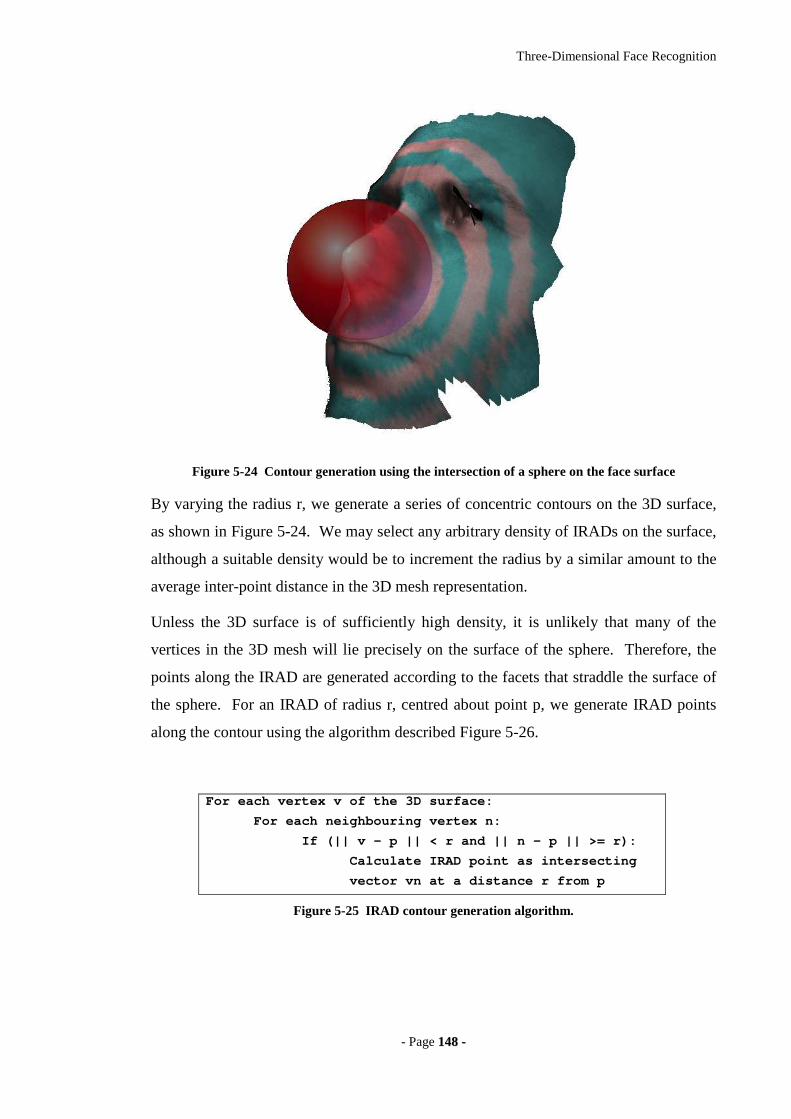
Three-Dimensional Face Recognition
- Page 114488 --
Figure 5-24 Contour generation using the intersection of a sphere on the face surface
By varying the radius r, we generate a series of concentric contours on the 3D surface,
as shown in Figure 5-24. We may select any arbitrary density of IRADs on the surface,
although a suitable density would be to increment the radius by a similar amount to the
average inter-point distance in the 3D mesh representation.
Unless the 3D surface is of sufficiently high density, it is unlikely that many of the
vertices in the 3D mesh will lie precisely on the surface of the sphere. Therefore, the
points along the IRAD are generated according to the facets that straddle the surface of
the sphere. For an IRAD of radius r, centred about point p, we generate IRAD points
along the contour using the algorithm described Figure 5-26.
For each vertex v of the 3D surface:
For each neighbouring vertex n:
If (|| v – p || < r and || n - p || >= r):
Calculate IRAD point as intersecting
vector vn at a distance r from p
Figure 5-25 IRAD contour generation algorithm.
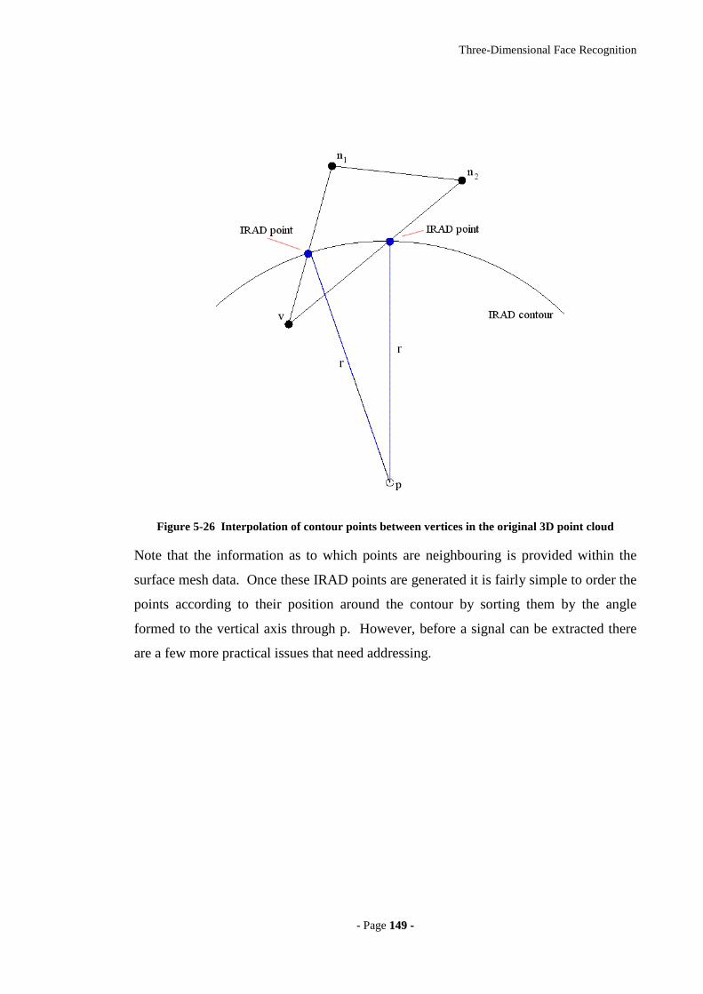
Three-Dimensional Face Recognition
- Page 114499 --
Figure 5-26 Interpolation of contour points between vertices in the original 3D point cloud
Note that the information as to which points are neighbouring is provided within the
surface mesh data. Once these IRAD points are generated it is fairly simple to order the
points according to their position around the contour by sorting them by the angle
formed to the vertical axis through p. However, before a signal can be extracted there
are a few more practical issues that need addressing.
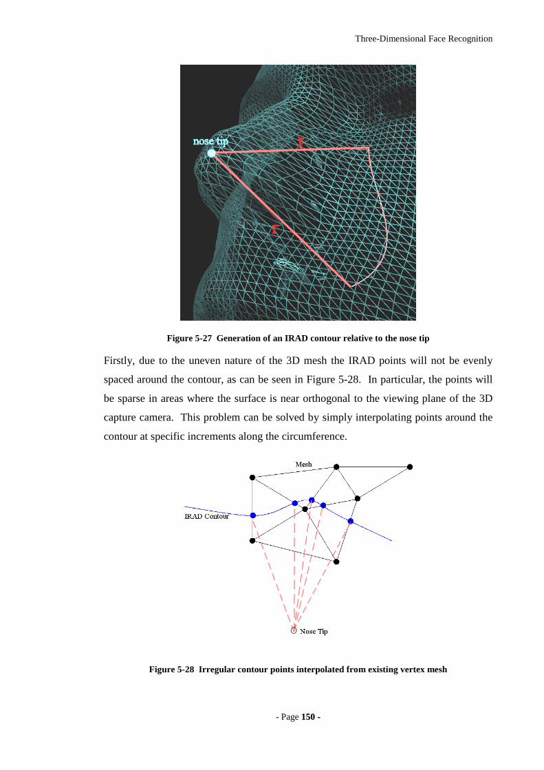
Three-Dimensional Face Recognition
- Page 115500 --
Figure 5-27 Generation of an IRAD contour relative to the nose tip
Firstly, due to the uneven nature of the 3D mesh the IRAD points will not be evenly
spaced around the contour, as can be seen in Figure 5-28. In particular, the points will
be sparse in areas where the surface is near orthogonal to the viewing plane of the 3D
capture camera. This problem can be solved by simply interpolating points around the
contour at specific increments along the circumference.
Figure 5-28 Irregular contour points interpolated from existing vertex mesh
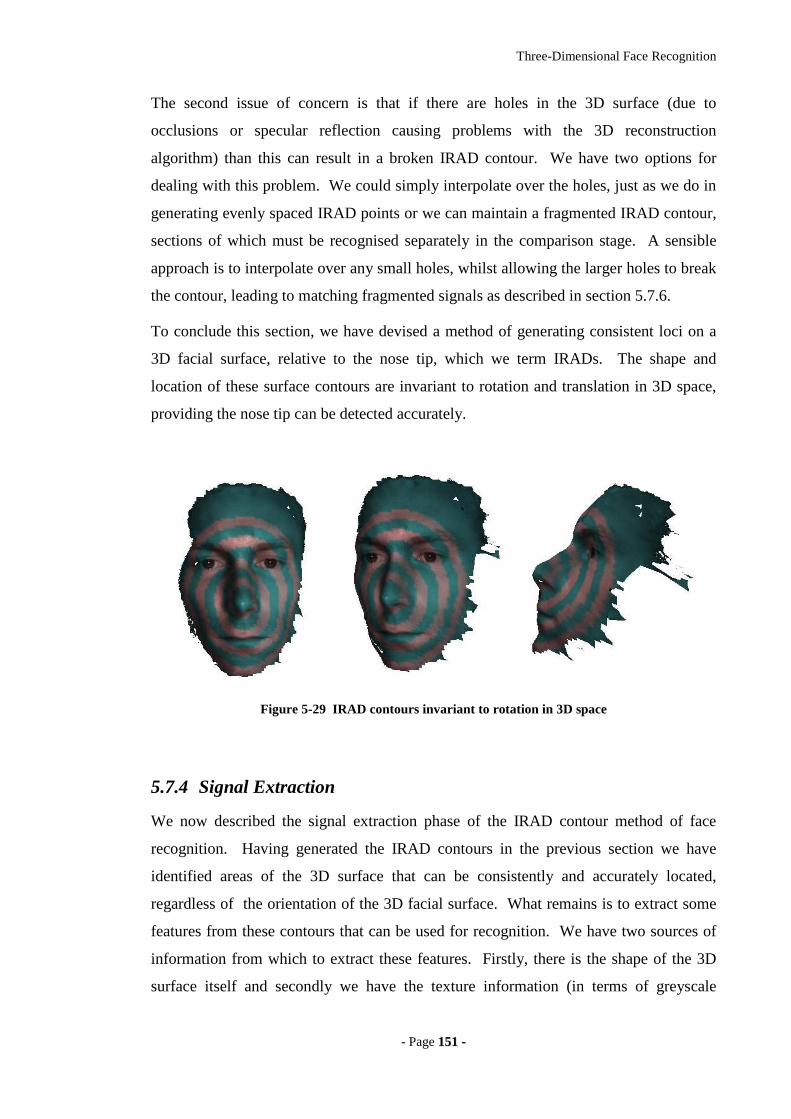
Three-Dimensional Face Recognition
- Page 115511 --
The second issue of concern is that if there are holes in the 3D surface (due to
occlusions or specular reflection causing problems with the 3D reconstruction
algorithm) than this can result in a broken IRAD contour. We have two options for
dealing with this problem. We could simply interpolate over the holes, just as we do in
generating evenly spaced IRAD points or we can maintain a fragmented IRAD contour,
sections of which must be recognised separately in the comparison stage. A sensible
approach is to interpolate over any small holes, whilst allowing the larger holes to break
the contour, leading to matching fragmented signals as described in section 5.7.6.
To conclude this section, we have devised a method of generating consistent loci on a
3D facial surface, relative to the nose tip, which we term IRADs. The shape and
location of these surface contours are invariant to rotation and translation in 3D space,
providing the nose tip can be detected accurately.
Figure 5-29 IRAD contours invariant to rotation in 3D space
5.7.4 Signal Extraction
We now described the signal extraction phase of the IRAD contour method of face
recognition. Having generated the IRAD contours in the previous section we have
identified areas of the 3D surface that can be consistently and accurately located,
regardless of the orientation of the 3D facial surface. What remains is to extract some
features from these contours that can be used for recognition. We have two sources of
information from which to extract these features. Firstly, there is the shape of the 3D
surface itself and secondly we have the texture information (in terms of greyscale
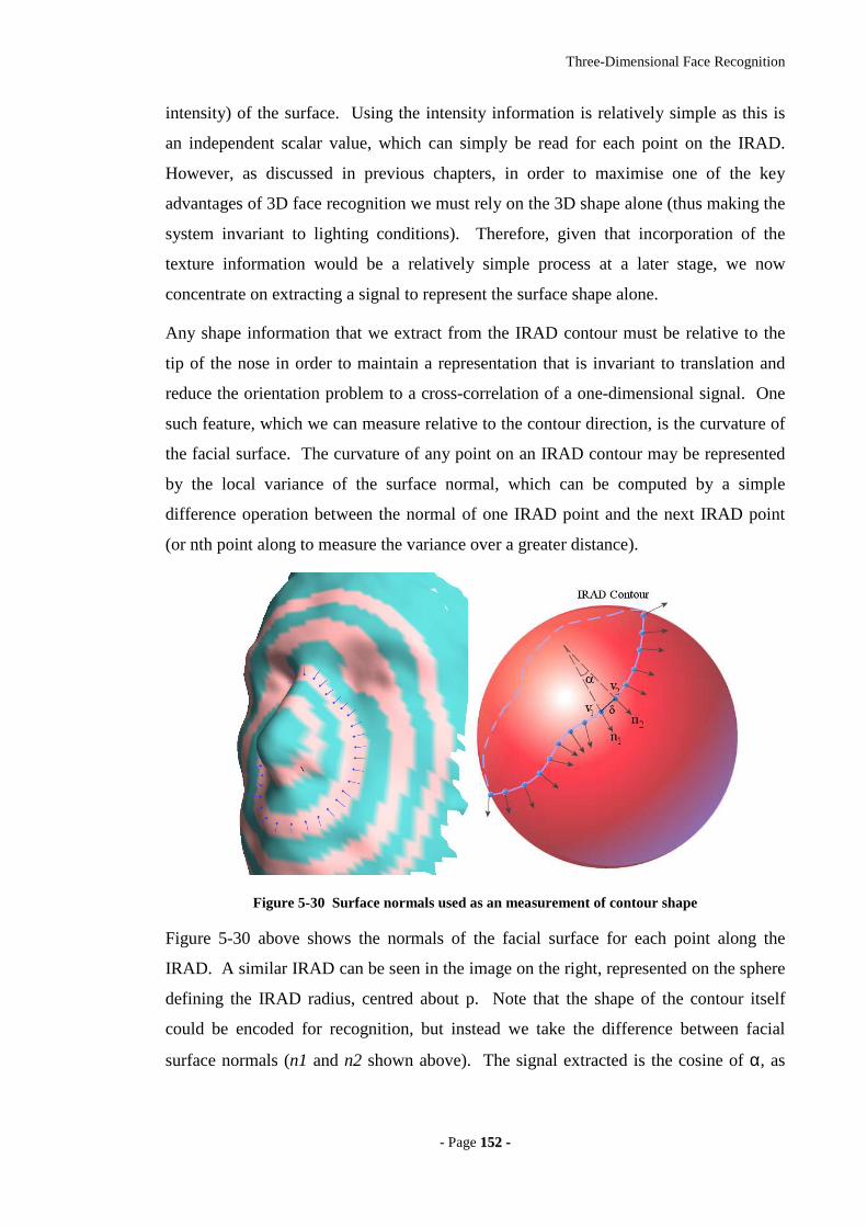
Three-Dimensional Face Recognition
- Page 115522 --
intensity) of the surface. Using the intensity information is relatively simple as this is
an independent scalar value, which can simply be read for each point on the IRAD.
However, as discussed in previous chapters, in order to maximise one of the key
advantages of 3D face recognition we must rely on the 3D shape alone (thus making the
system invariant to lighting conditions). Therefore, given that incorporation of the
texture information would be a relatively simple process at a later stage, we now
concentrate on extracting a signal to represent the surface shape alone.
Any shape information that we extract from the IRAD contour must be relative to the
tip of the nose in order to maintain a representation that is invariant to translation and
reduce the orientation problem to a cross-correlation of a one-dimensional signal. One
such feature, which we can measure relative to the contour direction, is the curvature of
the facial surface. The curvature of any point on an IRAD contour may be represented
by the local variance of the surface normal, which can be computed by a simple
difference operation between the normal of one IRAD point and the next IRAD point
(or nth point along to measure the variance over a greater distance).
Figure 5-30 Surface normals used as an measurement of contour shape
Figure 5-30 above shows the normals of the facial surface for each point along the
IRAD. A similar IRAD can be seen in the image on the right, represented on the sphere
defining the IRAD radius, centred about p. Note that the shape of the contour itself
could be encoded for recognition, but instead we take the difference between facial
surface normals (n1 and n2 shown above). The signal extracted is the cosine of α, as
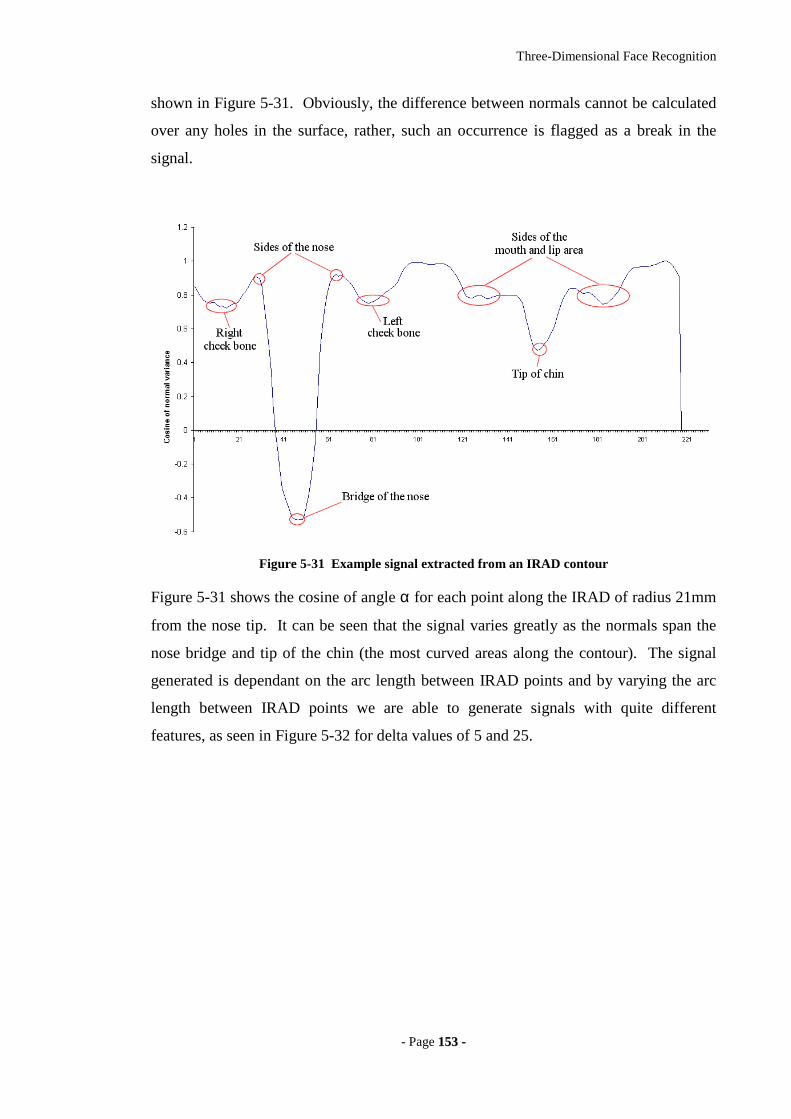
Three-Dimensional Face Recognition
- Page 115533 --
shown in Figure 5-31. Obviously, the difference between normals cannot be calculated
over any holes in the surface, rather, such an occurrence is flagged as a break in the
signal.
Figure 5-31 Example signal extracted from an IRAD contour
Figure 5-31 shows the cosine of angle α for each point along the IRAD of radius 21mm
from the nose tip. It can be seen that the signal varies greatly as the normals span the
nose bridge and tip of the chin (the most curved areas along the contour). The signal
generated is dependant on the arc length between IRAD points and by varying the arc
length between IRAD points we are able to generate signals with quite different
features, as seen in Figure 5-32 for delta values of 5 and 25.
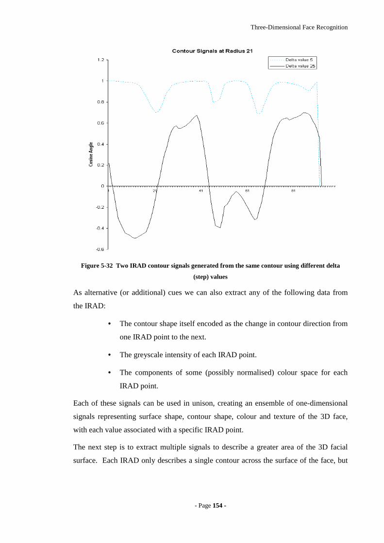
Three-Dimensional Face Recognition
- Page 115544 --
Figure 5-32 Two IRAD contour signals generated from the same contour using different delta
(step) values
As alternative (or additional) cues we can also extract any of the following data from
the IRAD:
• The contour shape itself encoded as the change in contour direction from
one IRAD point to the next.
• The greyscale intensity of each IRAD point.
• The components of some (possibly normalised) colour space for each
IRAD point.
Each of these signals can be used in unison, creating an ensemble of one-dimensional
signals representing surface shape, contour shape, colour and texture of the 3D face,
with each value associated with a specific IRAD point.
The next step is to extract multiple signals to describe a greater area of the 3D facial
surface. Each IRAD only describes a single contour across the surface of the face, but
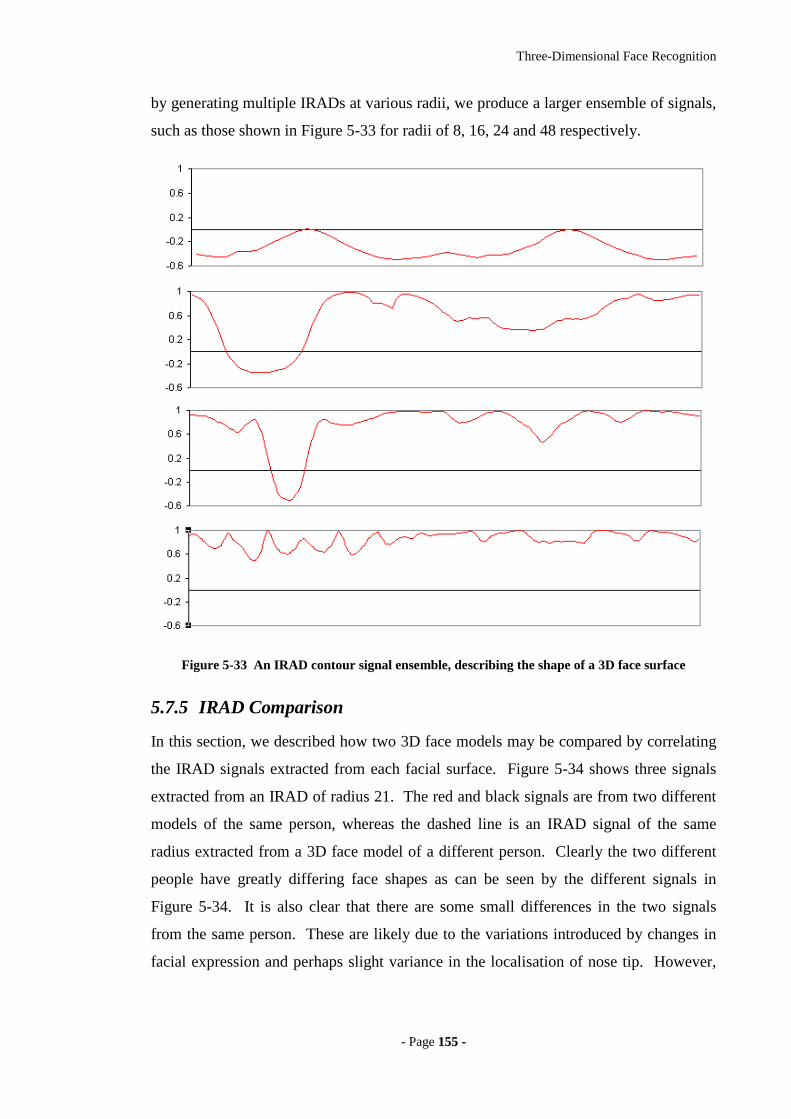
Three-Dimensional Face Recognition
- Page 115555 --
by generating multiple IRADs at various radii, we produce a larger ensemble of signals,
such as those shown in Figure 5-33 for radii of 8, 16, 24 and 48 respectively.
Figure 5-33 An IRAD contour signal ensemble, describing the shape of a 3D face surface
5.7.5 IRAD Comparison
In this section, we described how two 3D face models may be compared by correlating
the IRAD signals extracted from each facial surface. Figure 5-34 shows three signals
extracted from an IRAD of radius 21. The red and black signals are from two different
models of the same person, whereas the dashed line is an IRAD signal of the same
radius extracted from a 3D face model of a different person. Clearly the two different
people have greatly differing face shapes as can be seen by the different signals in
Figure 5-34. It is also clear that there are some small differences in the two signals
from the same person. These are likely due to the variations introduced by changes in
facial expression and perhaps slight variance in the localisation of nose tip. However,
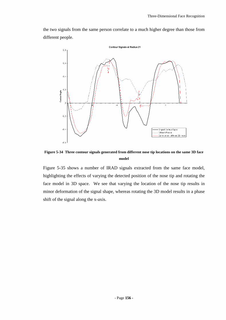
Three-Dimensional Face Recognition
- Page 115566 --
the two signals from the same person correlate to a much higher degree than those from
different people.
Figure 5-34 Three contour signals generated from different nose tip locations on the same 3D face
model
Figure 5-35 shows a number of IRAD signals extracted from the same face model,
highlighting the effects of varying the detected position of the nose tip and rotating the
face model in 3D space. We see that varying the location of the nose tip results in
minor deformation of the signal shape, whereas rotating the 3D model results in a phase
shift of the signal along the x-axis.
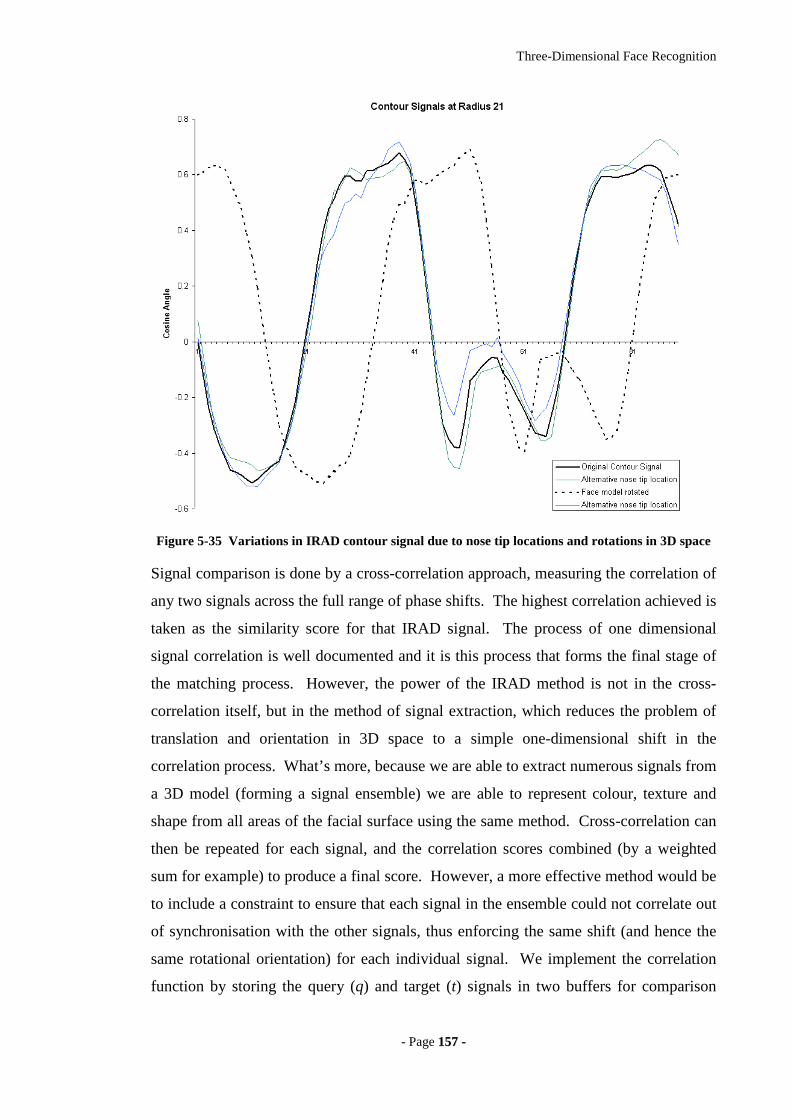
Three-Dimensional Face Recognition
- Page 115577 --
Figure 5-35 Variations in IRAD contour signal due to nose tip locations and rotations in 3D space
Signal comparison is done by a cross-correlation approach, measuring the correlation of
any two signals across the full range of phase shifts. The highest correlation achieved is
taken as the similarity score for that IRAD signal. The process of one dimensional
signal correlation is well documented and it is this process that forms the final stage of
the matching process. However, the power of the IRAD method is not in the cross-
correlation itself, but in the method of signal extraction, which reduces the problem of
translation and orientation in 3D space to a simple one-dimensional shift in the
correlation process. What’s more, because we are able to extract numerous signals from
a 3D model (forming a signal ensemble) we are able to represent colour, texture and
shape from all areas of the facial surface using the same method. Cross-correlation can
then be repeated for each signal, and the correlation scores combined (by a weighted
sum for example) to produce a final score. However, a more effective method would be
to include a constraint to ensure that each signal in the ensemble could not correlate out
of synchronisation with the other signals, thus enforcing the same shift (and hence the
same rotational orientation) for each individual signal. We implement the correlation
function by storing the query (q) and target (t) signals in two buffers for comparison
Three-Dimensional Face Recognition
- Page 115588 --
using the standard normalised cross correlation formula shown below, while we
iteratively increment an offset on one buffer, recording the maximum correlation value
for each rotation r, until the offset is equal to the length of the buffer.
ttqq
tqC
TT
T
r+
=
Equ. 5-9
This process has a high time complexity and some speed optimisations would be
required in order to search very large datasets. One such technique would be to
increment the offset in larger steps, then repeat the calculation for offsets close to the N
best correlation scores from the first pass. It may also be worthwhile implementing the
function using specialised hardware, allowing extremely fast comparisons or making
use of the Fast Fourier Transform. Finally, a number of pre-filters could be used to
eliminate unlikely matches, prior to performing the full correlation procedure. Such a
technique would mean computing a set of features from an IRAD signal. These features
may include such values as the maximum and minimum amplitude of signal peaks and
troughs, signal frequencies and surface path length, as well as using functions across
multiple IRADs, such as the ratio of IRAD lengths. These pre-filtering criteria should
be applied as weak constraints, before computing the full signal correlation. The
tolerance thresholds on the criteria may be set according to the maximum expected
within-class deviation, in order to ensure that no possible matches are eliminated.
The final step in computing some likeness score between to IRAD signal ensembles is
to combine the correlation scores from multiple signals into a single unified score. In
this chapter we investigate four of the simplest methods of combination:
• The sum of correlation scores from all IRADs.
• The sum of normalised (such that moments are equal) scores.
• The sum of scores from a subset of the most discriminatory IRADs.
• A weighed sum of scores (inversely proportional to the IRAD radius).
However, we do note that these combination functions are relatively unsophisticated
and that much more effective methods of combination may be found with further
investigation. Such methods may include a weighting based on the frequency and
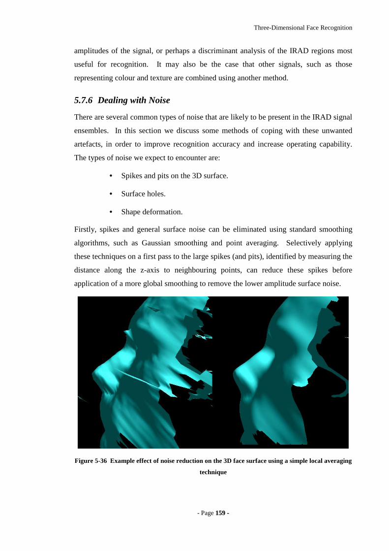
Three-Dimensional Face Recognition
- Page 115599 --
amplitudes of the signal, or perhaps a discriminant analysis of the IRAD regions most
useful for recognition. It may also be the case that other signals, such as those
representing colour and texture are combined using another method.
5.7.6 Dealing with Noise
There are several common types of noise that are likely to be present in the IRAD signal
ensembles. In this section we discuss some methods of coping with these unwanted
artefacts, in order to improve recognition accuracy and increase operating capability.
The types of noise we expect to encounter are:
• Spikes and pits on the 3D surface.
• Surface holes.
• Shape deformation.
Firstly, spikes and general surface noise can be eliminated using standard smoothing
algorithms, such as Gaussian smoothing and point averaging. Selectively applying
these techniques on a first pass to the large spikes (and pits), identified by measuring the
distance along the z-axis to neighbouring points, can reduce these spikes before
application of a more global smoothing to remove the lower amplitude surface noise.
Figure 5-36 Example effect of noise reduction on the 3D face surface using a simple local averaging
technique

Three-Dimensional Face Recognition
- Page 116600 --
Small holes in the surface resulting from missing polygons (typically due to failure in
finding a stereo correspondence) can easily be filled by computing an average central
point and connecting the mesh. However, larger holes occurring on one side of the
nose, because the subjects were facing to the left or right, or missing areas around the
eyes and forehead due to hair or glasses require a different approach. Our signal
matching procedure must be able to cope with partial signals, which do not complete a
loop on the surface. In Figure 5-37 below it can be seen how a complete signal would
be reduced to a partial signal as two unconnected surface areas. It is clear that the
partial signal would not fully correlate with the original signal. However, by splitting
the partial signal into two sub-signals at the point of the surface break, it is possible to
match the two sub-signals to a larger complete signal by correlating each one
individually. The rule applied in this scenario is to correlate partial signals in order of
signal length. Once a correlation is achieved, further correlations are performed using
any remaining sections of the signal not yet correlated.
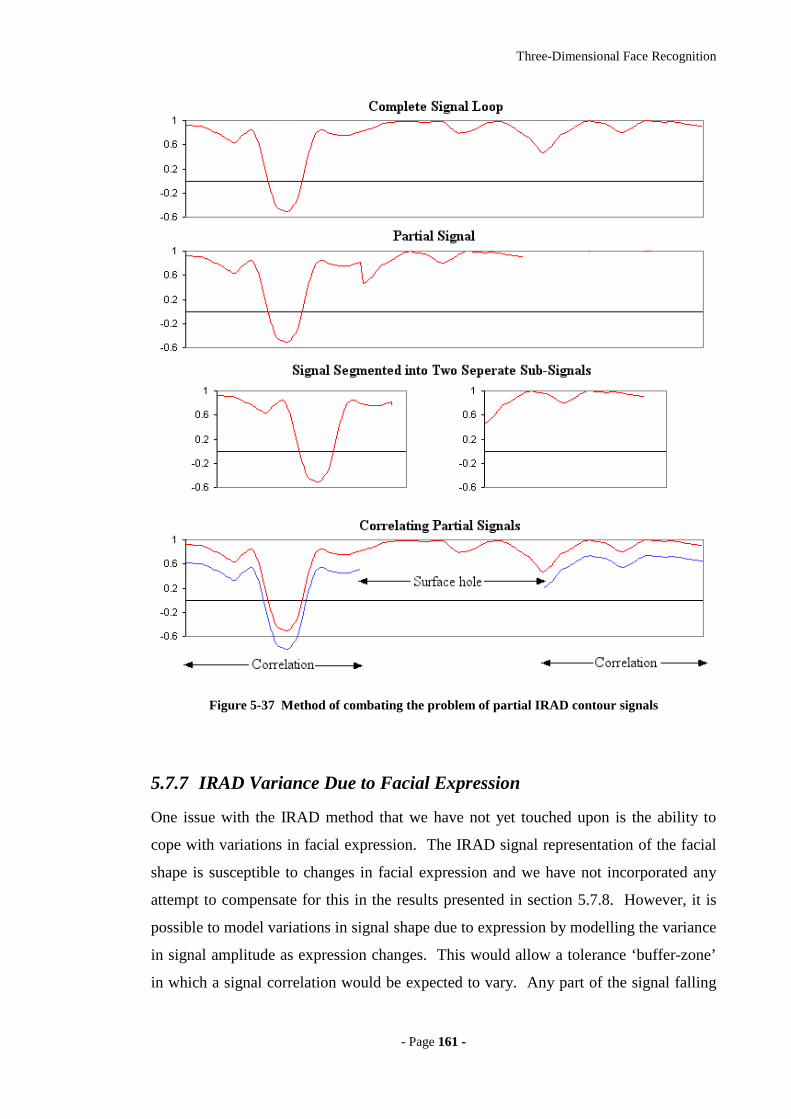
Three-Dimensional Face Recognition
- Page 116611 --
Figure 5-37 Method of combating the problem of partial IRAD contour signals
5.7.7 IRAD Variance Due to Facial Expression
One issue with the IRAD method that we have not yet touched upon is the ability to
cope with variations in facial expression. The IRAD signal representation of the facial
shape is susceptible to changes in facial expression and we have not incorporated any
attempt to compensate for this in the results presented in section 5.7.8. However, it is
possible to model variations in signal shape due to expression by modelling the variance
in signal amplitude as expression changes. This would allow a tolerance ‘buffer-zone’
in which a signal correlation would be expected to vary. Any part of the signal falling
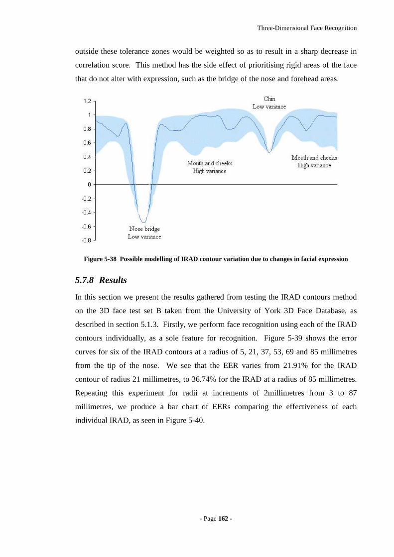
Three-Dimensional Face Recognition
- Page 116622 --
outside these tolerance zones would be weighted so as to result in a sharp decrease in
correlation score. This method has the side effect of prioritising rigid areas of the face
that do not alter with expression, such as the bridge of the nose and forehead areas.
Figure 5-38 Possible modelling of IRAD contour variation due to changes in facial expression
5.7.8 Results
In this section we present the results gathered from testing the IRAD contours method
on the 3D face test set B taken from the University of York 3D Face Database, as
described in section 5.1.3. Firstly, we perform face recognition using each of the IRAD
contours individually, as a sole feature for recognition. Figure 5-39 shows the error
curves for six of the IRAD contours at a radius of 5, 21, 37, 53, 69 and 85 millimetres
from the tip of the nose. We see that the EER varies from 21.91% for the IRAD
contour of radius 21 millimetres, to 36.74% for the IRAD at a radius of 85 millimetres.
Repeating this experiment for radii at increments of 2millimetres from 3 to 87
millimetres, we produce a bar chart of EERs comparing the effectiveness of each
individual IRAD, as seen in Figure 5-40.
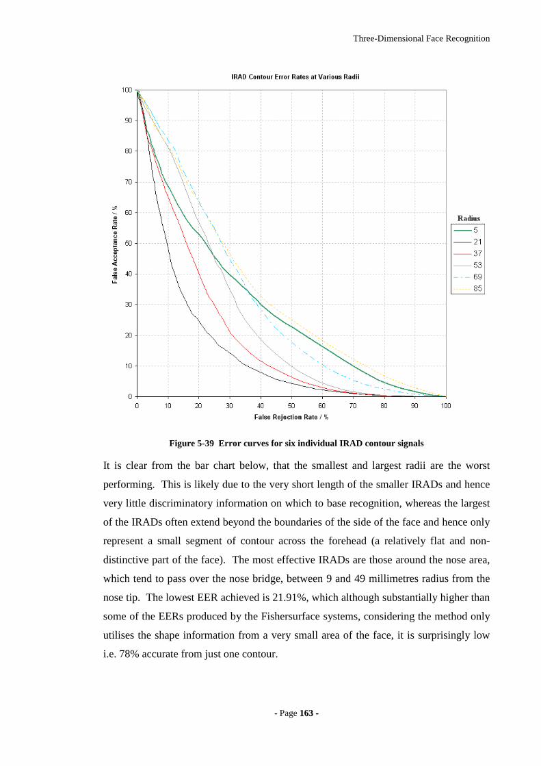
Three-Dimensional Face Recognition
- Page 116633 --
Figure 5-39 Error curves for six individual IRAD contour signals
It is clear from the bar chart below, that the smallest and largest radii are the worst
performing. This is likely due to the very short length of the smaller IRADs and hence
very little discriminatory information on which to base recognition, whereas the largest
of the IRADs often extend beyond the boundaries of the side of the face and hence only
represent a small segment of contour across the forehead (a relatively flat and non-
distinctive part of the face). The most effective IRADs are those around the nose area,
which tend to pass over the nose bridge, between 9 and 49 millimetres radius from the
nose tip. The lowest EER achieved is 21.91%, which although substantially higher than
some of the EERs produced by the Fishersurface systems, considering the method only
utilises the shape information from a very small area of the face, it is surprisingly low
i.e. 78% accurate from just one contour.

Three-Dimensional Face Recognition
- Page 116644 --
Figure 5-40 Bar chart of EER for each individual IRAD contour signal at various radii from the
nose tip
The next step is to combine the scores using the four methods described earlier, to base
the recognition on correlation of a signal ensemble (rather than a single IRAD).
However, to produce the results shown in Figure 5-41, we have not implemented the
rotational constraint that all IRADs must correlate ‘in-phase’. That is, the rotational
shift has been allowed to vary between signals i.e. the face is not considered as a rigid
body.
We see that summing the correlation scores from all IRADs produced, results in a
higher EER (25.40%) than using the best of the IRADs individually (21.91%). This
result is only marginally improved (to an EER of 23.12%) by normalising the scores
such that the average and standard deviation are equal for all signals prior to
combination. However, we have been successful in improving the EER (down to
20.56%) by summing only those scores from the best performing IRADs (at radii
between 9mm and 49mm). Finally, weighting the scores based on the inverse of the
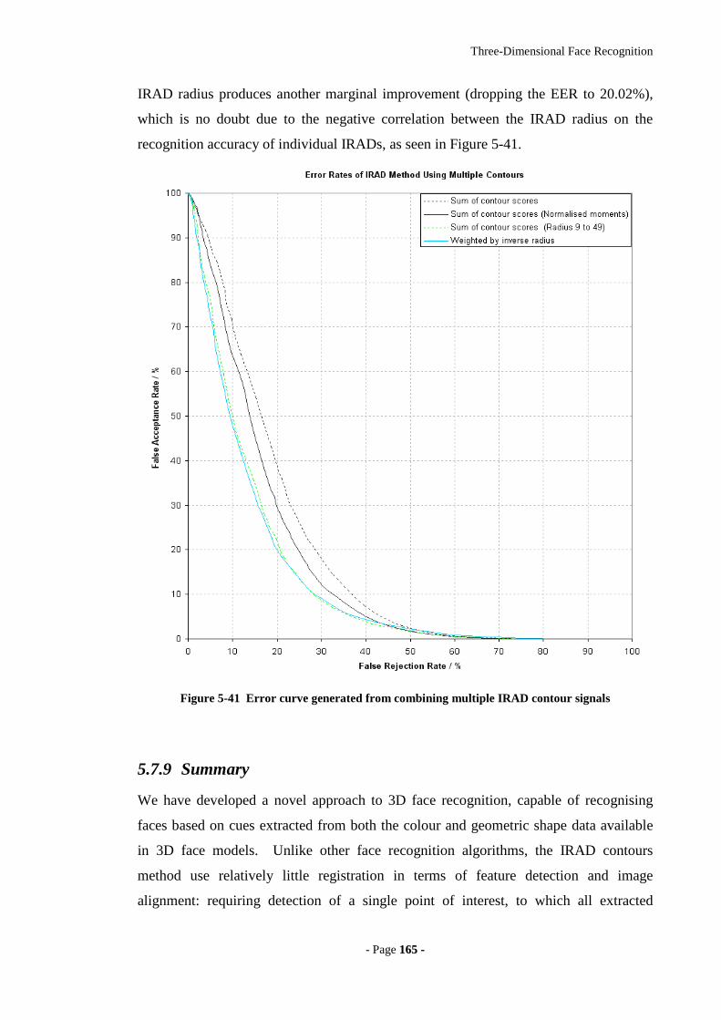
Three-Dimensional Face Recognition
- Page 116655 --
IRAD radius produces another marginal improvement (dropping the EER to 20.02%),
which is no doubt due to the negative correlation between the IRAD radius on the
recognition accuracy of individual IRADs, as seen in Figure 5-41.
Figure 5-41 Error curve generated from combining multiple IRAD contour signals
5.7.9 Summary
We have developed a novel approach to 3D face recognition, capable of recognising
faces based on cues extracted from both the colour and geometric shape data available
in 3D face models. Unlike other face recognition algorithms, the IRAD contours
method use relatively little registration in terms of feature detection and image
alignment: requiring detection of a single point of interest, to which all extracted

Three-Dimensional Face Recognition
- Page 116666 --
features are relative. In particular, the method reduces the problem of head orientation
to a one-dimensional shift in a simple cross-correlation process. The method is not only
applicable to faces, but can be used to recognise and register any 3D object. It may also
prove useful in providing the 3D model alignment required by other face recognition
methods, such as the Fishersurface method described in section 5.6.
Utilising the nose tip detection algorithm developed in previous sections, we have
demonstrated the application of the IRAD contours method to face recognition, using
geometric shape information alone, to produce signal ensembles from a range of
contours on the facial surface. The effectiveness of each contour for recognition is
dependant on the distance from the point of interest (in this case the nose tip), with
contours in the region between the nostrils and cheekbone being the most effective.
Experimentation with combining the scores from each signal in a signal ensemble has
shown that recognition accuracy can be improved by utilising signals extracted from
multiple IRAD contours. However, we have only applied very simple weighted sums in
order to achieve this improvement and it is likely that much greater reductions in error
rate could be achieved by using a more sophisticated weighting technique (perhaps
having been trained using an additional set of 3D face data). In addition to these
improvements, a further increase in accuracy is likely to occur when addition
information is extracted from the IRAD contours, such as colour and texture data.
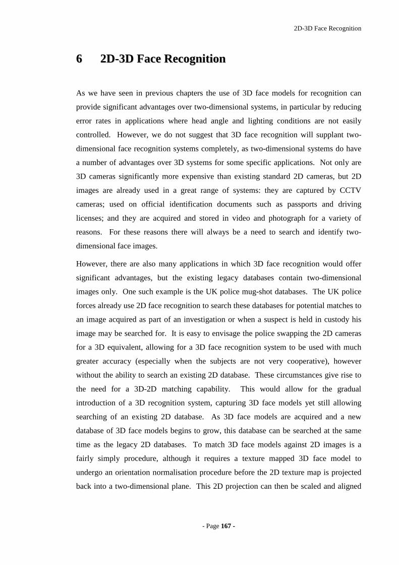
2D-3D Face Recognition
- Page 116677 --
66 22DD--33DD FFaaccee RReeccooggnnii tt iioonn
As we have seen in previous chapters the use of 3D face models for recognition can
provide significant advantages over two-dimensional systems, in particular by reducing
error rates in applications where head angle and lighting conditions are not easily
controlled. However, we do not suggest that 3D face recognition will supplant two-
dimensional face recognition systems completely, as two-dimensional systems do have
a number of advantages over 3D systems for some specific applications. Not only are
3D cameras significantly more expensive than existing standard 2D cameras, but 2D
images are already used in a great range of systems: they are captured by CCTV
cameras; used on official identification documents such as passports and driving
licenses; and they are acquired and stored in video and photograph for a variety of
reasons. For these reasons there will always be a need to search and identify two-
dimensional face images.
However, there are also many applications in which 3D face recognition would offer
significant advantages, but the existing legacy databases contain two-dimensional
images only. One such example is the UK police mug-shot databases. The UK police
forces already use 2D face recognition to search these databases for potential matches to
an image acquired as part of an investigation or when a suspect is held in custody his
image may be searched for. It is easy to envisage the police swapping the 2D cameras
for a 3D equivalent, allowing for a 3D face recognition system to be used with much
greater accuracy (especially when the subjects are not very cooperative), however
without the ability to search an existing 2D database. These circumstances give rise to
the need for a 3D-2D matching capability. This would allow for the gradual
introduction of a 3D recognition system, capturing 3D face models yet still allowing
searching of an existing 2D database. As 3D face models are acquired and a new
database of 3D face models begins to grow, this database can be searched at the same
time as the legacy 2D databases. To match 3D face models against 2D images is a
fairly simply procedure, although it requires a texture mapped 3D face model to
undergo an orientation normalisation procedure before the 2D texture map is projected
back into a two-dimensional plane. This 2D projection can then be scaled and aligned

2D-3D Face Recognition
- Page 116688 --
according to the eye locations and matched against a standard 2D image using the
techniques already discussed in section 4.
66..11 RReeccooggnnii tt iioonn UUssiinngg 33DD TTeexxttuurr ee MM aapp PPrr oojj eecctt iioonnss
In this section we explore another approach to face recognition that falls somewhere
between the two-dimensional and 3D approaches discussed so far, in that is uses the 3D
face model in order to perform orientation normalisation, before performing recognition
based on the two-dimensional texture data. Whereas the 3D systems explored in section
5 have all been intentionally applied to geometric structure alone (in order to become
invariant to lighting conditions). It may be that if the lighting conditions can be
controlled to some extent, then by ignoring the two-dimensional colour data held in the
texture map we are discarding a wealth of highly discriminatory information that could
be useful for recognition. We do address these issues in section 7.4, by reintroducing
the 2D texture information in combining two-dimensional and 3D systems. However, if
an existing 2D face recognition system is already in place, perhaps highly optimised for
specific circumstances (for a certain race under specific lighting conditions for
example), it may be preferential to continue using the two-dimensional system, rather
than gathering the necessary training data to optimise a new 3D system. Under these
circumstances it is still possible to gain some of the advantages offered by a 3D system
by utilising the 3D camera, without necessarily performing recognition on the surface
shape, but rely purely on the 2D texture map. Such a system would become more
resistant to variations in head orientation, yet still use the underlying 2D recognition
algorithm.
In order to implement such a system, the 3D camera would generate a texture mapped
3D face model, which would then undergo the orientation normalisation procedure
described in section 5.2. The texture of the resultant fronto-parallel 3D face model can
then be projected onto a 2D plane, creating a standard 2D image of the face. As well as
having the advantage of normalising head orientation this system also introduces two
other significant advantages. Firstly, the resultant image is to scale, meaning that the
actual size of the head and distance between the eyes can be used as features for
recognition. Secondly, because the orientation normalisation algorithm has already
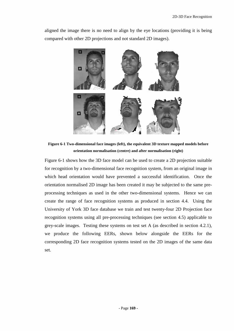
2D-3D Face Recognition
- Page 116699 --
aligned the image there is no need to align by the eye locations (providing it is being
compared with other 2D projections and not standard 2D images).
Figure 6-1 Two-dimensional face images (left), the equivalent 3D texture mapped models before
orientation normalisation (centre) and after normalisation (right)
Figure 6-1 shows how the 3D face model can be used to create a 2D projection suitable
for recognition by a two-dimensional face recognition system, from an original image in
which head orientation would have prevented a successful identification. Once the
orientation normalised 2D image has been created it may be subjected to the same pre-
processing techniques as used in the other two-dimensional systems. Hence we can
create the range of face recognition systems as produced in section 4.4. Using the
University of York 3D face database we train and test twenty-four 2D Projection face
recognition systems using all pre-processing techniques (see section 4.5) applicable to
grey-scale images. Testing these systems on test set A (as described in section 4.2.1),
we produce the following EERs, shown below alongside the EERs for the
corresponding 2D face recognition systems tested on the 2D images of the same data
set.
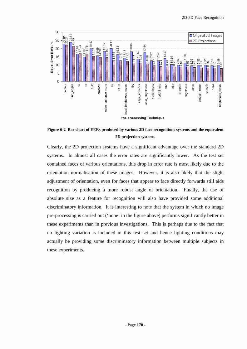
2D-3D Face Recognition
- Page 117700 --
Figure 6-2 Bar chart of EERs produced by various 2D face recognitions systems and the equivalent
2D projection systems.
Clearly, the 2D projection systems have a significant advantage over the standard 2D
systems. In almost all cases the error rates are significantly lower. As the test set
contained faces of various orientations, this drop in error rate is most likely due to the
orientation normalisation of these images. However, it is also likely that the slight
adjustment of orientation, even for faces that appear to face directly forwards still aids
recognition by producing a more robust angle of orientation. Finally, the use of
absolute size as a feature for recognition will also have provided some additional
discriminatory information. It is interesting to note that the system in which no image
pre-processing is carried out (‘none’ in the figure above) performs significantly better in
these experiments than in previous investigations. This is perhaps due to the fact that
no lighting variation is included in this test set and hence lighting conditions may
actually be providing some discriminatory information between multiple subjects in
these experiments.
Combining Methods of Face Recognition
- Page 117711 --
77 CCoommbbiinniinngg MM eetthhooddss ooff FFaaccee RReeccooggnnii tt iioonn
Up to this point we have discussed various approaches to face recognition and methods
of improving the performance of these systems by applying such things as image pre-
processing techniques and various distance metrics. We have also shown that the use of
3D face models can offer significant advantages over the 2D face images, thus
producing a new generation of face recognition systems, again using a variety of pre-
processing techniques to produce a variety of surface representations. These face
recognition systems has each been evaluated by producing the EER for a given test set,
resulting in a large range of error rates. What we have not considered, until this point,
is that each system may have its own advantages under certain conditions, or that
although one system may not perform well in terms of EERs, it may contain, within its
extracted feature space, some discriminating factor not considered in other systems that
use a different image (or surface) representation.
In this section we introduce methods of combining multiple face recognition systems,
hoping to consolidate the advantages of numerous systems into a single unified system
that outperforms any of its individual components. We begin by combining two-
dimensional face recognition systems in section 7.1, computing the best combinations
of eigenface and Fisherface systems, when applied to the AR face database of 2D
images. We then apply a similar strategy to 3D Fishersurface systems, testing both the
cosine and Euclidean distance measures in section 7.2. These two investigations lead
naturally to the combining of two-dimensional and 3D systems, creating a unified face
recognition method that utilises both 3D geometric structure as well as colour and
texture information. Such a system is presented in section 7.4.
We introduce some new terminology in this section that deserves some clarification.
We describe the method of amalgamating multiple face recognition systems as
‘subspace combination’ and the resultant combined subspace as a ‘composite subspace.’
When referring to a complete face recognition system that utilises a composite subspace
it is often termed a ‘multi-subspace system’ in contrast with the ‘single-subspace
systems’ described in previous chapters. Note that in many of the charts and figures we
use the abbreviation ‘combo X’ to denote a multi-subspace system in which
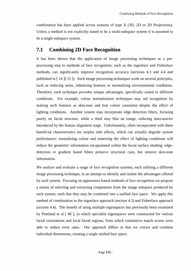
Combining Methods of Face Recognition
- Page 117722 --
combination has been applied across systems of type X (3D, 2D or 2D Projections).
Unless a method is not explicitly stated to be a multi-subspace system it is assumed to
be a single-subspace system.
77..11 CCoommbbiinniinngg 22DD FFaaccee RReeccooggnnii tt iioonn
It has been shown that the application of image processing techniques as a pre-
processing step to methods of face recognition, such as the eigenface and Fisherface
methods, can significantly improve recognition accuracy (sections 4.3 and 4.4 and
published in [ 14 ][ 15 ]). Such image processing techniques work on several principles,
such as reducing noise, enhancing features or normalising environmental conditions.
Therefore, each technique provides unique advantages, specifically suited to different
conditions. For example, colour normalisation techniques may aid recognition by
making such features as skin-tone and hair colour consistent despite the effect of
lighting conditions. Another system may incorporate edge detection filters, focusing
purely on facial structure, while a third may blur an image, reducing inaccuracies
introduced by the feature alignment stage. Unfortunately, often incorporated with these
beneficial characteristics are surplus side effects, which can actually degrade system
performance: normalising colour and removing the effect of lighting conditions will
reduce the geometric information encapsulated within the facial surface shading; edge-
detection or gradient based filters preserve structural cues, but remove skin-tone
information.
We analyse and evaluate a range of face recognition systems, each utilising a different
image processing technique, in an attempt to identify and isolate the advantages offered
by each system. Focusing on appearance based methods of face recognition we propose
a means of selecting and extracting components from the image subspace produced by
each system, such that they may be combined into a unified face space. We apply this
method of combination to the eigenface approach (section 4.3) and Fisherface approach
(section 4.4). The benefit of using multiple eigenspaces has previously been examined
by Pentland et al [ 40 ], in which specialist eigenspaces were constructed for various
facial orientations and local facial regions, from which cumulative match scores were
able to reduce error rates. Our approach differs in that we extract and combine
individual dimensions, creating a single unified face space.
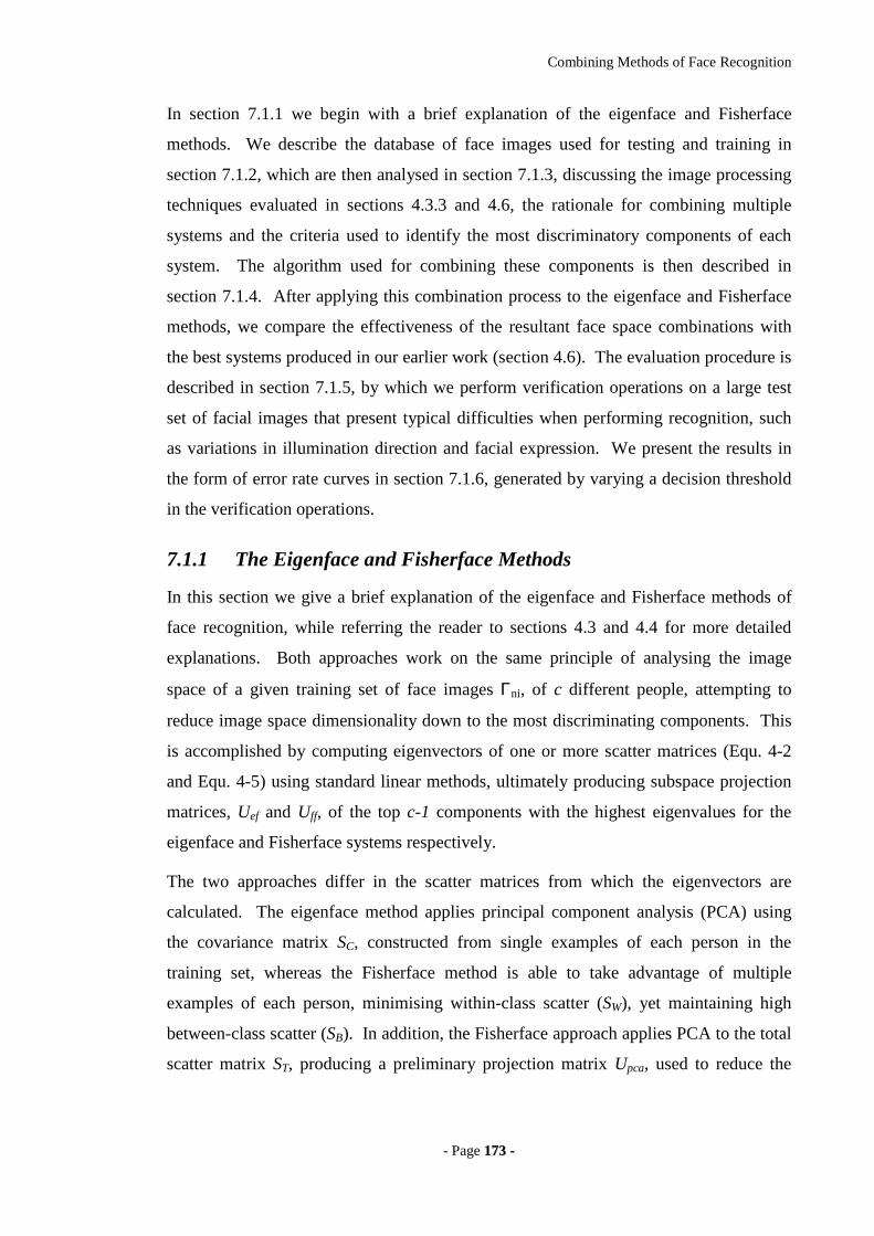
Combining Methods of Face Recognition
- Page 117733 --
In section 7.1.1 we begin with a brief explanation of the eigenface and Fisherface
methods. We describe the database of face images used for testing and training in
section 7.1.2, which are then analysed in section 7.1.3, discussing the image processing
techniques evaluated in sections 4.3.3 and 4.6, the rationale for combining multiple
systems and the criteria used to identify the most discriminatory components of each
system. The algorithm used for combining these components is then described in
section 7.1.4. After applying this combination process to the eigenface and Fisherface
methods, we compare the effectiveness of the resultant face space combinations with
the best systems produced in our earlier work (section 4.6). The evaluation procedure is
described in section 7.1.5, by which we perform verification operations on a large test
set of facial images that present typical difficulties when performing recognition, such
as variations in illumination direction and facial expression. We present the results in
the form of error rate curves in section 7.1.6, generated by varying a decision threshold
in the verification operations.
7.1.1 The Eigenface and Fisherface Methods
In this section we give a brief explanation of the eigenface and Fisherface methods of
face recognition, while referring the reader to sections 4.3 and 4.4 for more detailed
explanations. Both approaches work on the same principle of analysing the image
space of a given training set of face images Γni, of c different people, attempting to
reduce image space dimensionality down to the most discriminating components. This
is accomplished by computing eigenvectors of one or more scatter matrices (Equ. 4-2
and Equ. 4-5) using standard linear methods, ultimately producing subspace projection
matrices, Uef and Uff, of the top c-1 components with the highest eigenvalues for the
eigenface and Fisherface systems respectively.
The two approaches differ in the scatter matrices from which the eigenvectors are
calculated. The eigenface method applies principal component analysis (PCA) using
the covariance matrix SC, constructed from single examples of each person in the
training set, whereas the Fisherface method is able to take advantage of multiple
examples of each person, minimising within-class scatter (SW), yet maintaining high
between-class scatter (SB). In addition, the Fisherface approach applies PCA to the total
scatter matrix ST, producing a preliminary projection matrix Upca, used to reduce the
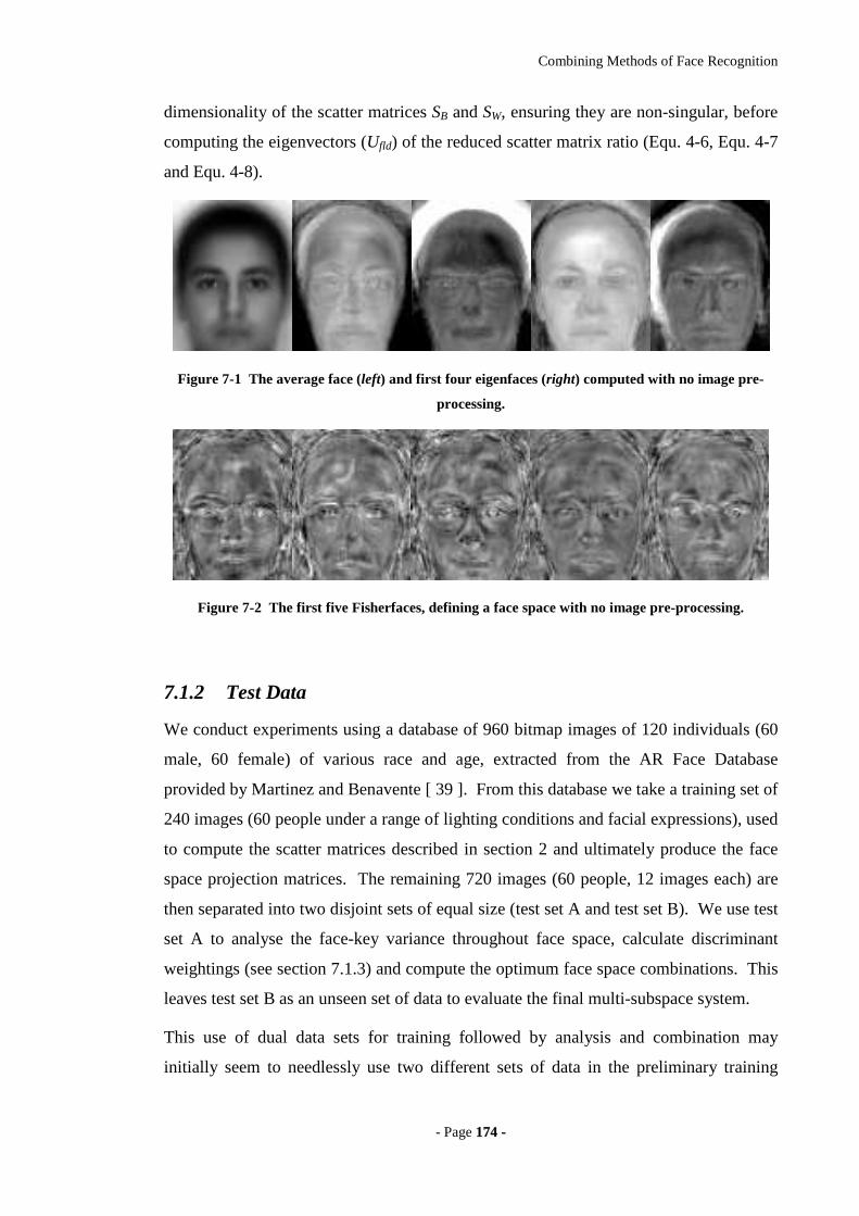
Combining Methods of Face Recognition
- Page 117744 --
dimensionality of the scatter matrices SB and SW, ensuring they are non-singular, before
computing the eigenvectors (Ufld) of the reduced scatter matrix ratio (Equ. 4-6, Equ. 4-7
and Equ. 4-8).
Figure 7-1 The average face (left) and first four eigenfaces (right) computed with no image pre-
processing.
Figure 7-2 The first five Fisherfaces, defining a face space with no image pre-processing.
7.1.2 Test Data
We conduct experiments using a database of 960 bitmap images of 120 individuals (60
male, 60 female) of various race and age, extracted from the AR Face Database
provided by Martinez and Benavente [ 39 ]. From this database we take a training set of
240 images (60 people under a range of lighting conditions and facial expressions), used
to compute the scatter matrices described in section 2 and ultimately produce the face
space projection matrices. The remaining 720 images (60 people, 12 images each) are
then separated into two disjoint sets of equal size (test set A and test set B). We use test
set A to analyse the face-key variance throughout face space, calculate discriminant
weightings (see section 7.1.3) and compute the optimum face space combinations. This
leaves test set B as an unseen set of data to evaluate the final multi-subspace system.
This use of dual data sets for training followed by analysis and combination may
initially seem to needlessly use two different sets of data in the preliminary training
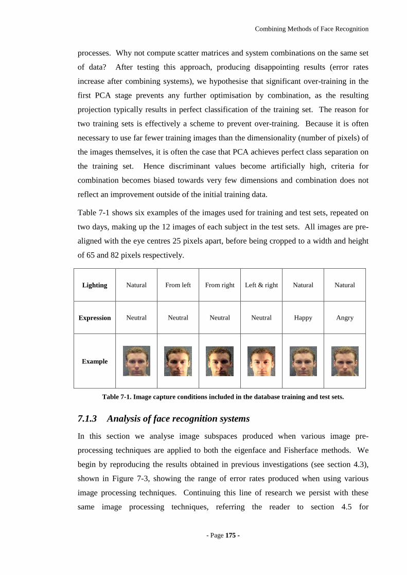
Combining Methods of Face Recognition
- Page 117755 --
processes. Why not compute scatter matrices and system combinations on the same set
of data? After testing this approach, producing disappointing results (error rates
increase after combining systems), we hypothesise that significant over-training in the
first PCA stage prevents any further optimisation by combination, as the resulting
projection typically results in perfect classification of the training set. The reason for
two training sets is effectively a scheme to prevent over-training. Because it is often
necessary to use far fewer training images than the dimensionality (number of pixels) of
the images themselves, it is often the case that PCA achieves perfect class separation on
the training set. Hence discriminant values become artificially high, criteria for
combination becomes biased towards very few dimensions and combination does not
reflect an improvement outside of the initial training data.
Table 7-1 shows six examples of the images used for training and test sets, repeated on
two days, making up the 12 images of each subject in the test sets. All images are pre-
aligned with the eye centres 25 pixels apart, before being cropped to a width and height
of 65 and 82 pixels respectively.
Lighting Natural From left From right Left & right Natural Natural
Expression Neutral Neutral Neutral Neutral Happy Angry
Example
Table 7-1. Image capture conditions included in the database training and test sets.
7.1.3 Analysis of face recognition systems
In this section we analyse image subspaces produced when various image pre-
processing techniques are applied to both the eigenface and Fisherface methods. We
begin by reproducing the results obtained in previous investigations (see section 4.3),
shown in Figure 7-3, showing the range of error rates produced when using various
image processing techniques. Continuing this line of research we persist with these
same image processing techniques, referring the reader to section 4.5 for

Combining Methods of Face Recognition
- Page 117766 --
implementation details, while here we focus on the effect and methodologies of
combining multiple systems, rather than the image processing techniques themselves.
Figure 7-3 clearly shows that the choice of image processing technique has a significant
effect on the performance of both the eigenface and Fisherface approaches, with detail
enhancement filters providing the lowest EER when used in conjunction with the
Fisherface approach. However, we find it surprising that some image processing
techniques give such poor performance, especially when designed specifically to
compensate for conditions known to be a source of error in face recognition systems.
For example, we see that intensity normalisation increases error rates for Fisherface-
based systems, despite being the best performing image processing technique for
eigenface-based recognition. Hence, it is apparent that this processing technique is able
to preserve discriminatory information, while normalising lighting effects, yet is
unsuitable for Fisherface-based recognition. We now carry out further investigation
into the discriminating ability of each face recognition system by applying Fisher’s
Linear Discriminant (FLD), as used by Gordon [ 4 ] to analyse 3D face features, to
individual components (single dimensions) of each face space. Focusing on a single
face space dimension we calculate the discriminant d, describing the discriminating
power of that dimension, between c people in test set A.
∑ ∑
∑
= Φ∈Φ
=
−
−=
c
i xi
c
ii
i
imx
mmd
1
21
1
2
)(
)(
Equ. 7-1
Where m is the mean value of that dimension in the face-keys of test set A, mi the
within-class mean of class i and i the set of vector elements taken from the face-keys
of class i.
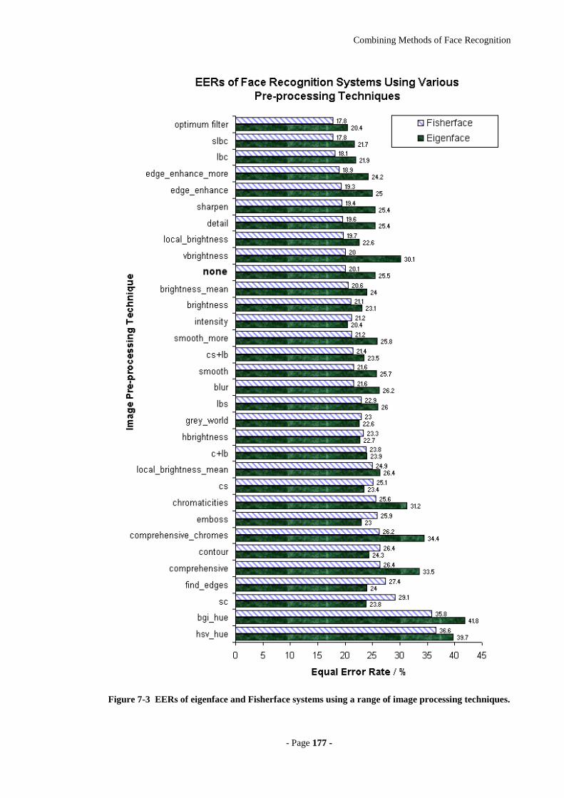
Combining Methods of Face Recognition
- Page 117777 --
Figure 7-3 EERs of eigenface and Fisherface systems using a range of image processing techniques.

Combining Methods of Face Recognition
- Page 117788 --
Applying Equ. 7-1 to each dimension of the eigenface face space (using no image pre-
processing), provides a set of discriminant values as shown in Figure 7-4. Looking at
the range of discriminant values, we note that the higher discriminants appear at the
lower end of the face space. This is exactly as we would expect, showing that the order
of principal components, in terms of eigenvalues, is broadly related to that dimensions
discriminating ability.
Figure 7-4 Discriminant values of the eigenface face space dimensions using no image pre-
processing.
However, it can also be seen that certain dimensions produce very low discriminant
values. In Figure 7-4 we see that the third principal component in particular has a very
low discriminating ability, despite its relatively high eigenvalue. This highlights some
problems in the eigenface training method, in that the third dimension obviously
represents something of high variance in the training set that has little or no use in
discriminating between different people. In other words, it is a feature of the
environmental capture conditions. Applying Equ. 7-1 to each dimension in the
assortment of Fisherface systems, we see similar results to those of the eigenface
systems, with a wide range of discriminant values across the different image processing
techniques. Figure 7-5 shows the top ten dimensions with the highest discriminant
value from each Fisherface system.
It is clear that although some image processing techniques do not perform well in the
face recognition tests, producing high EERs as seen in Figure 7-3 some of their face-key
components do contain highly discriminatory information. We hypothesise that the
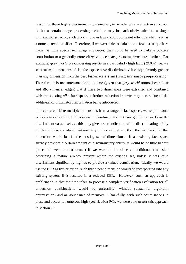
Combining Methods of Face Recognition
- Page 117799 --
reason for these highly discriminating anomalies, in an otherwise ineffective subspace,
is that a certain image processing technique may be particularly suited to a single
discriminating factor, such as skin tone or hair colour, but is not effective when used as
a more general classifier. Therefore, if we were able to isolate these few useful qualities
from the more specialised image subspaces, they could be used to make a positive
contribution to a generally more effective face space, reducing error rates further. For
example, grey_world pre-processing results in a particularly high EER (23.0%), yet we
see that two dimensions of this face space have discriminant values significantly greater
than any dimension from the best Fisherface system (using slbc image pre-processing).
Therefore, it is not unreasonable to assume (given that grey_world normalises colour
and slbc enhances edges) that if these two dimensions were extracted and combined
with the existing slbc face space, a further reduction in error may occur, due to the
additional discriminatory information being introduced.
In order to combine multiple dimensions from a range of face spaces, we require some
criterion to decide which dimensions to combine. It is not enough to rely purely on the
discriminant value itself, as this only gives us an indication of the discriminating ability
of that dimension alone, without any indication of whether the inclusion of this
dimension would benefit the existing set of dimensions. If an existing face space
already provides a certain amount of discriminatory ability, it would be of little benefit
(or could even be detrimental) if we were to introduce an additional dimension
describing a feature already present within the existing set, unless it was of a
discriminant significantly high as to provide a valued contribution. Ideally we would
use the EER as this criterion, such that a new dimension would be incorporated into any
existing system if it resulted in a reduced EER. However, such an approach is
problematic in that the time taken to process a complete verification evaluation for all
dimension combinations would be unfeasible, without substantial algorithm
optimisations and an abundance of memory. Thankfully, with such optimisations in
place and access to numerous high specification PCs, we were able to test this approach
in section 7.3.
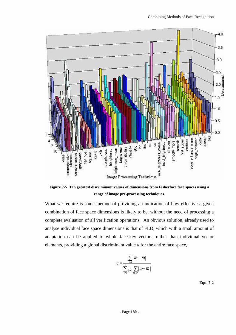
Combining Methods of Face Recognition
- Page 118800 --
Figure 7-5 Ten greatest discriminant values of dimensions from Fisherface face spaces using a
range of image pre-processing techniques.
What we require is some method of providing an indication of how effective a given
combination of face space dimensions is likely to be, without the need of processing a
complete evaluation of all verification operations. An obvious solution, already used to
analyse individual face space dimensions is that of FLD, which with a small amount of
adaptation can be applied to whole face-key vectors, rather than individual vector
elements, providing a global discriminant value d for the entire face space,
∑ ∑
∑
= Φ∈Φ
=
−
−=
c
ii
c
ii
i
i
d
1
1
1
ωωω
ωω
Equ. 7-2

Combining Methods of Face Recognition
- Page 118811 --
where ω is the face-key of some single or combined face space, to which we apply the
distance metric to the averageω and class average iω . Applying Equ. 7-2 to each
Fisherface system shown in Figure 7-3 and comparing the result with their respective
EERs, it becomes evident there is some correlation between this global discriminant
value and the effectiveness of a face recognition system, as seen in Figure 7-6.
Figure 7-6 Scatter graph showing the correlation between the global discriminant value and EER
of Fisherface systems.
7.1.4 Combining Systems
In this section we describe how the analysis methods discussed in section 7.1.3 are used
to combine multiple face recognition systems. Firstly, we need to address the problem
of prioritising face space dimensions. Because the average magnitude and deviation of
face-key vectors from a range of systems are likely to differ by some orders of
magnitude, certain dimensions will have a greater influence than others, even if the
discriminating abilities are evenly matched. To compensate for this effect, we
normalise moments by dividing each face-key element by its within-class standard

Combining Methods of Face Recognition
- Page 118822 --
deviation. However, in normalising these dimensions we have also removed any
prioritisation, such that all face space components are considered equal. Although not a
problem when applied to a single face space, when combining multiple dimensions we
would ideally wish to give greater precedence to the more reliable components.
Otherwise the situation is likely to arise when a large number of less discriminating (but
still useful) dimensions begin to outweigh the fewer more discriminating ones,
diminishing their influence on the verification operation and hence increasing error
rates.
In section 7.1.3 we showed how FLD could be used to measure the discriminating
ability of a single dimension from any given face space. We now apply this
discriminant value d (Equ. 7-1) as a weighting for each face space dimension,
prioritising those dimensions with the highest discriminating ability.
With this weighting scheme applied to all face-keys produced by each system, we can
begin to combine dimensions into a single unified face space. The criterion required for
a new dimension to be introduced to an existing face space is a resultant increase in the
global discriminant, calculated using Equ. 7-2. However, as can be seen from Figure
7-6 this method can only provide a rough indication of system effectiveness and if we
were to build up the combination from a single dimension, we may achieve a greater
discriminant but not necessarily the lowest EER. Therefore, in order to provide the
combination with the best head start, we initialise the dimension set with the best face
space achieved so far (intensity and slbc for eigenface and Fisherface systems
respectively). Beginning with this small preliminary set of dimensions (the face space
of the best eigenface or Fisherface system), we then iteratively test each additional
dimension from other face spaces for combination with the existing dimension set as
shown in the ‘combination by accumulation’ algorithm below.
The result is a new face space consisting of the dimensions taken from the best single
subspace system, plus a selection of additional dimensions from other systems. Each
new dimension will have increased the global discriminant, such that the final
combination has a significantly higher discriminant value and will therefore also have
reduced the EER when evaluated on test set B.
Combining Methods of Face Recognition
- Page 118833 --
Composite face space = face space dimensions of best single system
Calculate global FLD of composite face space
For each face space system:
For each dimension of face space system:
Concatenate new dimension onto composite face space
Calculate global FLD of composite face space
If global FLD has not increased:
Remove new dimension from composite face space
Save composite face space ready for evaluation
Figure 7-7 Face space dimensional combination by accumulation algorithm, based on an FLD
fitness criteria.
7.1.5 The Test Procedure
The effectiveness of the face recognition systems is evaluated by means of error rate
curves (FRR vs. FAR) generated by performing a large number of verification
operations on the database test sets. The images in the test set are verified against every
other image, producing a distance value. No image is compared with itself and each
pair is compared only once (the relationship is symmetric). This provides 64,620
verification operations when performed on all images in test set B or 258,840 operations
if both test sets A and B are combined. After calculating the distance values for each
comparison, a threshold is applied in order to derive the rejection/acceptance decision
for each image pair. FAR is calculated as the percentage of acceptance decisions when
images of different people are compared and FRR is the percentage of rejection
decisions when images of the same person are compared. By varying the threshold we
produce a set of FRR FAR plots, forming the error rate curve, as shown in Figure 7-9.
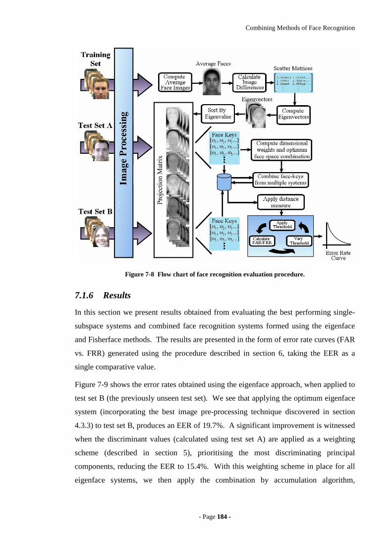
Combining Methods of Face Recognition
- Page 118844 --
Figure 7-8 Flow chart of face recognition evaluation procedure.
7.1.6 Results
In this section we present results obtained from evaluating the best performing single-
subspace systems and combined face recognition systems formed using the eigenface
and Fisherface methods. The results are presented in the form of error rate curves (FAR
vs. FRR) generated using the procedure described in section 6, taking the EER as a
single comparative value.
Figure 7-9 shows the error rates obtained using the eigenface approach, when applied to
test set B (the previously unseen test set). We see that applying the optimum eigenface
system (incorporating the best image pre-processing technique discovered in section
4.3.3) to test set B, produces an EER of 19.7%. A significant improvement is witnessed
when the discriminant values (calculated using test set A) are applied as a weighting
scheme (described in section 5), prioritising the most discriminating principal
components, reducing the EER to 15.4%. With this weighting scheme in place for all
eigenface systems, we then apply the combination by accumulation algorithm,
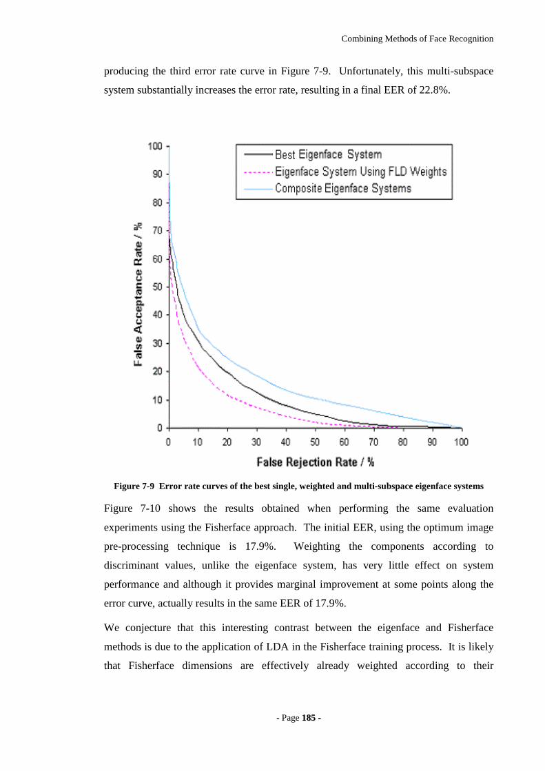
Combining Methods of Face Recognition
- Page 118855 --
producing the third error rate curve in Figure 7-9. Unfortunately, this multi-subspace
system substantially increases the error rate, resulting in a final EER of 22.8%.
Figure 7-9 Error rate curves of the best single, weighted and multi-subspace eigenface systems
Figure 7-10 shows the results obtained when performing the same evaluation
experiments using the Fisherface approach. The initial EER, using the optimum image
pre-processing technique is 17.9%. Weighting the components according to
discriminant values, unlike the eigenface system, has very little effect on system
performance and although it provides marginal improvement at some points along the
error curve, actually results in the same EER of 17.9%.
We conjecture that this interesting contrast between the eigenface and Fisherface
methods is due to the application of LDA in the Fisherface training process. It is likely
that Fisherface dimensions are effectively already weighted according to their
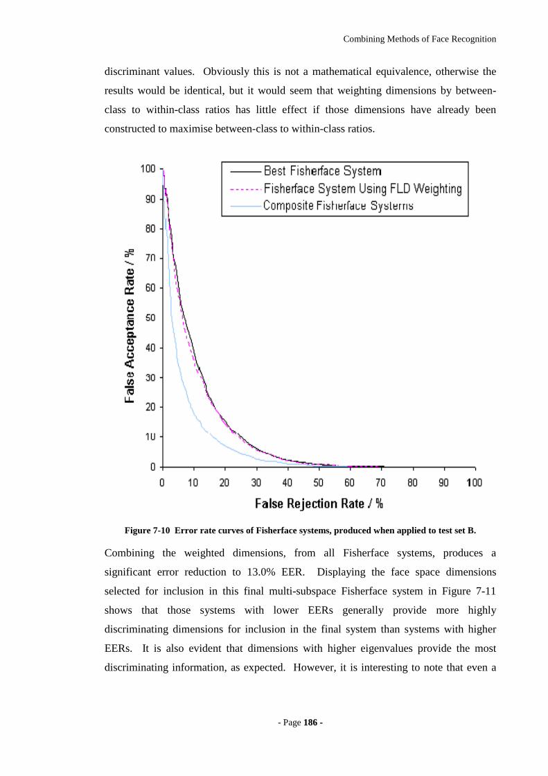
Combining Methods of Face Recognition
- Page 118866 --
discriminant values. Obviously this is not a mathematical equivalence, otherwise the
results would be identical, but it would seem that weighting dimensions by between-
class to within-class ratios has little effect if those dimensions have already been
constructed to maximise between-class to within-class ratios.
Figure 7-10 Error rate curves of Fisherface systems, produced when applied to test set B.
Combining the weighted dimensions, from all Fisherface systems, produces a
significant error reduction to 13.0% EER. Displaying the face space dimensions
selected for inclusion in this final multi-subspace Fisherface system in Figure 7-11
shows that those systems with lower EERs generally provide more highly
discriminating dimensions for inclusion in the final system than systems with higher
EERs. It is also evident that dimensions with higher eigenvalues provide the most
discriminating information, as expected. However, it is interesting to note that even a
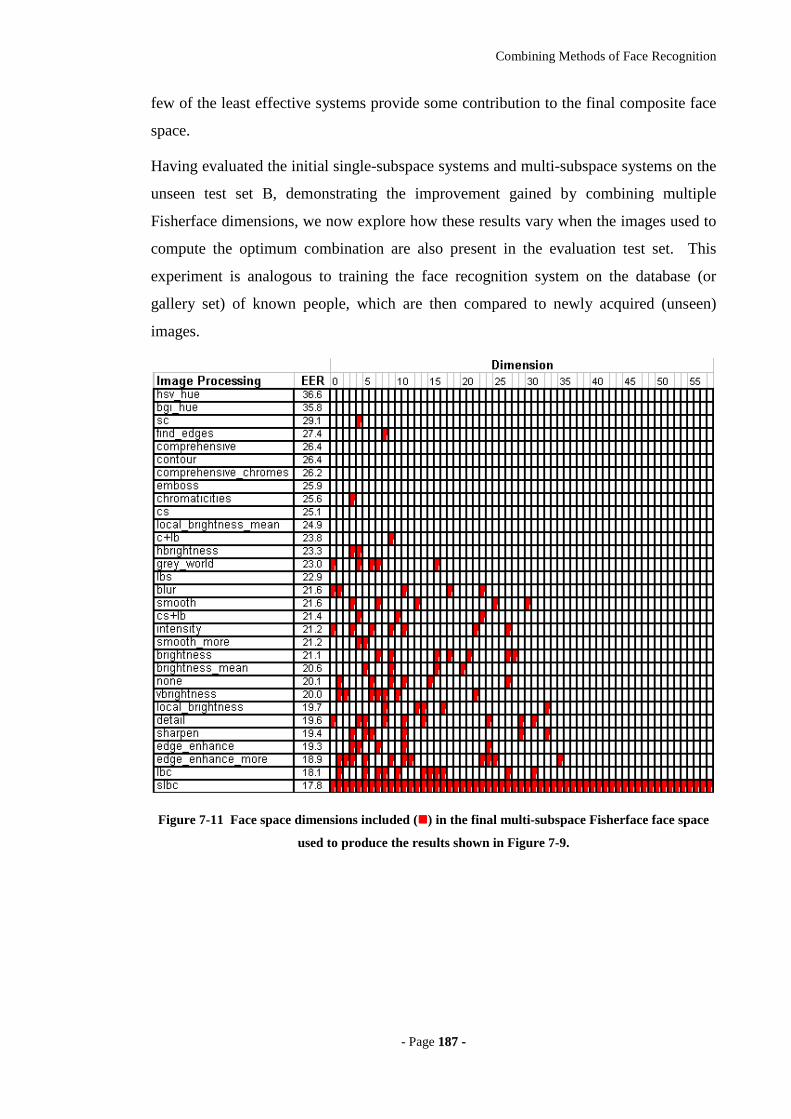
Combining Methods of Face Recognition
- Page 118877 --
few of the least effective systems provide some contribution to the final composite face
space.
Having evaluated the initial single-subspace systems and multi-subspace systems on the
unseen test set B, demonstrating the improvement gained by combining multiple
Fisherface dimensions, we now explore how these results vary when the images used to
compute the optimum combination are also present in the evaluation test set. This
experiment is analogous to training the face recognition system on the database (or
gallery set) of known people, which are then compared to newly acquired (unseen)
images.
Figure 7-11 Face space dimensions included () in the final multi-subspace Fisherface face space
used to produce the results shown in Figure 7-9.
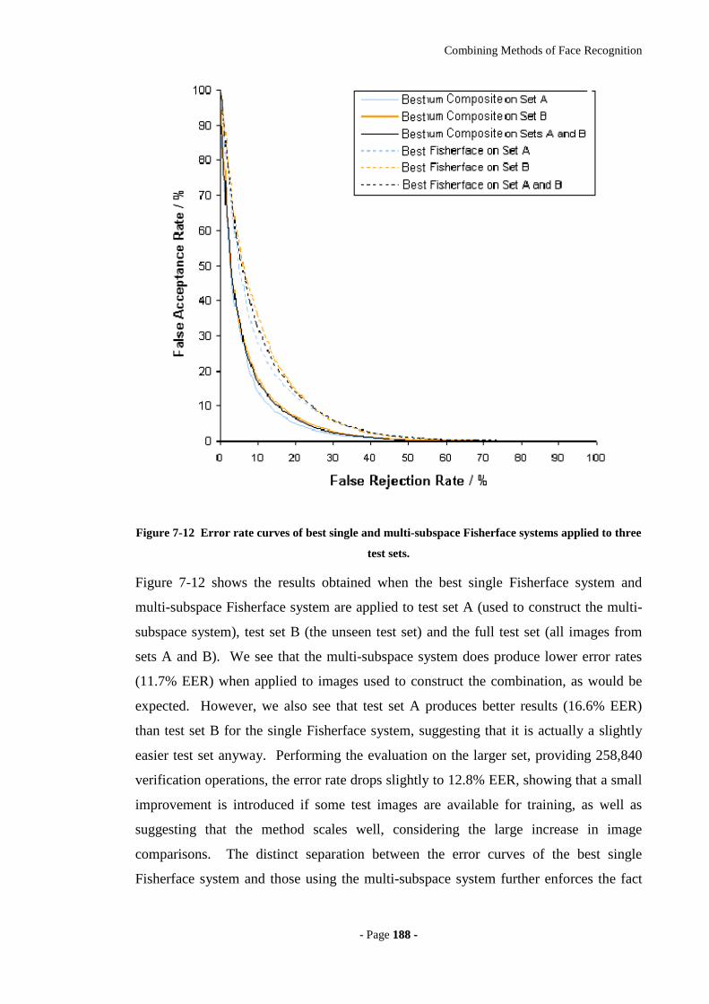
Combining Methods of Face Recognition
- Page 118888 --
Figure 7-12 Error rate curves of best single and multi-subspace Fisherface systems applied to three
test sets.
Figure 7-12 shows the results obtained when the best single Fisherface system and
multi-subspace Fisherface system are applied to test set A (used to construct the multi-
subspace system), test set B (the unseen test set) and the full test set (all images from
sets A and B). We see that the multi-subspace system does produce lower error rates
(11.7% EER) when applied to images used to construct the combination, as would be
expected. However, we also see that test set A produces better results (16.6% EER)
than test set B for the single Fisherface system, suggesting that it is actually a slightly
easier test set anyway. Performing the evaluation on the larger set, providing 258,840
verification operations, the error rate drops slightly to 12.8% EER, showing that a small
improvement is introduced if some test images are available for training, as well as
suggesting that the method scales well, considering the large increase in image
comparisons. The distinct separation between the error curves of the best single
Fisherface system and those using the multi-subspace system further enforces the fact
Combining Methods of Face Recognition
- Page 118899 --
that combining multiple face space dimensions provides a substantial advantage over
individual systems that use a single image processing technique.
7.1.7 Conclusion
We have highlighted the importance of using image processing as a pre-processing step
to two well-known methods of face recognition (eigenface and Fisherface) and
discussed the possibilities of combining face space dimensions of multiple systems in
an attempt to utilise the advantages offered by numerous image processing techniques.
Using FLD as an analysis tool we have confirmed the hypothesis that although an image
subspace may not perform well when used for recognition, it may harbour highly
discriminatory components that could complement other more superior systems and
hence we have shown the potential to improve recognition error rates by combining
multiple dimensions from a range of face recognition systems.
Using this method of FLD analysis, we have overcome two problems presented when
combining face recognition systems. Firstly, using the respective discriminant values to
weight face space dimensions, according to their discriminating ability, has allowed us
to combine multiple dimensions yet maintain a bias towards those that present the most
distinguishing features. We have shown this weighting scheme to be highly beneficial
when used with the best single eigenface system, reducing the EER from 19.7% to
15.4%, but have little influence on the effectiveness of individual Fisherface systems
(probably because the subspace computation process has already accounted for
between-class to within-class ratios). Secondly, applying FLD to entire face-keys and
comparing these global discriminant values with the EERs of existing systems has
demonstrated how this analysis can be used to provide a rough indication of the
effectiveness of a given face recognition system, requiring significantly less processing
time than completing a full set of verification operations on the same data. Using this
global discriminant as criteria for selecting face space dimensions as potential sources
of additional discriminatory information to an existing system has enabled an iterative
approach of appending new face space dimensions to existing combinations, increasing
the global discriminant value and hence improving the performance of the multi-
subspace face recognition system.
Combining Methods of Face Recognition
- Page 119900 --
Testing this method of combination on face space representations produced using the
eigenface approach has shown it to be ineffective for this method of face recognition,
increasing the EER significantly from 15.4% to 22.8%. However, applying the same
combination process to Fisherface systems has shown that combining multiple face
spaces can improve system performance substantially, reducing the EER from 17.9%
down to 13.0%.
This key difference between the eigenface and Fisherface approaches is of particular
interest and at first thought perhaps quite surprising. In order to understand this
phenomenon, we must consider the method of combination used. We have created a
criterion in which face space dimensions are incorporated into an existing set if they
increase the discriminant of the composite face space. This criterion only takes into
account the discriminating ability of the new dimension when compared with the level
of discrimination already achieved within the existing combination. It does not allow
for the inter-dependency of features or the possibility that features represented in the
additional dimension may already be present in the existing combination face space.
For example, consider a composite face space, in which its current set of dimensions
encapsulates such features as the nose base width, bridge curvature and nose length.
Now suppose we identify a new dimension for inclusion in the face space, representing
the more general feature of nose shape, which due to its high between-class variance
will increases the global discriminant. However, this new dimension represents a
feature that is largely dependent on those already represented in the face space.
Therefore the discriminatory information available in this new dimension is
predominantly redundant, meaning that the only real contribution to the multi-subspace
system is the additional noise of within-class variance.
This reasoning begins to uncover the grounds for failing to successfully combine
multiple eigenface systems. The eigenface approach creates a face space that
maximises image distribution, but uses no examples of within-class variance, therefore
doing nothing to reduce noise or environmental features. Any dimension combined
with an existing face space not only introduces the primary discriminating feature
(which may have been present beforehand anyway) but also incorporates substantial
within-class variance. Adini et al [ 26 ] have shown that differences due to lighting
conditions and facial expression are greater than the differences between images of

Combining Methods of Face Recognition
- Page 119911 --
different people, suggesting that the noise introduced when combining dimensions will
be more diverse and cumulative than the discriminating features, which will often
reoccur and hence be redundant. The Fisherface approach differs in its ability to
formulate face space such that within-class variation is minimised relative to between-
class variation, hence reducing environmental influence, allowing multiple dimensions
to combine with relatively little increase in noise content. Therefore, even if the
dimension contribution is redundant, little degradation is introduced.
The criterion used to select dimensions is obviously an important factor in the
combination process. In this section we develop a method of using FLD to predict
system effectiveness, which due to its short processing time allows many combinations
to be tested in a relatively small amount of time, yet we see from Figure 7-6 that the
system with the greatest discriminant value does not necessarily have the lowest EER.
Therefore it is highly likely that other face space combinations exist that will produce a
lower EER than the best combination presented so far in the thesis. Such a face space
combination could easily be found if a more accurate representation of system
effectiveness was used in the combination selection criteria. One obvious choice is the
EER itself. Although this would take an extremely long time to process, once the
dimensions have been identified, the multi-subspace projection matrix can be stored for
latter use and providing the training set is sufficiently large and varied, re-training and
re-combining would not be required.
We have already shown that image processing improves the Fisherface method of face
recognition from an EER of 20.1% using no image processing, to 17.8% using the best
processing technique. We have extended this line of research to show that creating a
face space combination, incorporating multiple Fisherface systems reduces the EER
further, down to 12.8% when tested on a large amount of data presenting typical
difficulties when performing recognition. Evaluating this system at its fundamental
level, using 258,840 verification operations between face images, demonstrates that
combining multiple face space dimensions improves the effectiveness of the core face
recognition engine. We have not applied any additional heuristics, typically
incorporated into fully functional commercial and industrial systems. For example, we
have not experimented with different distance metrics, multiple facial alignments,
optimising crop regions or storing multiple gallery images. All of which are known to

Combining Methods of Face Recognition
- Page 119922 --
improve error rates and can easily be applied to the multi-subspace face recognition
systems presented here. With these additional measures in place, it is likely that the
improvements made to the core recognition engine will bring the error rates of fully
functional commercial and industrial systems substantially closer to those required for
the application scenarios in mind.
Combining Methods of Face Recognition
- Page 119933 --
77..22 CCoommbbiinniinngg 33DD FFaaccee RReeccooggnnii tt iioonn
In section 5.3 we demonstrated how the use of various surface representations affects
the performance of 3D face recognition systems and in analysing these various filtering
techniques we have seen how the discriminating abilities vary. What we have not
considered, until now, is how these various representations may be combined to further
advantage.
In this section we expand on earlier investigations involving the use of facial surface
data, derived from 3D face models (generated using a stereo vision 3D camera), as a
substitute for the more familiar two-dimensional images. Previous investigations
(section 5.5 and published in [ 16 ]), have shown how different surface representations
and distance measures affect recognition, reducing the EER from 19.1% to 12.7% when
applied to a difficult test set of 290 face models. However, the focus of this research
has been on identifying optimum surface representations, with little regard for the
advantages offered by each individual representation.
We suggest that different surface representations may be specifically suited to different
capture conditions or certain facial characteristics, despite a general weakness for
overall recognition. For example, curvature representations may aid recognition by
making the system more robust to inaccuracies in 3D orientation but are highly sensitive
to noise. Another representation may enhance nose shape, but lose information
regarding jaw structure.
We now carry out similar investigations as those applied to two-dimensional
recognition in section 7.1 and published by Heseltine et al [ 35 ]. We analyse and
evaluate a variety of 3D Fishersurface [ 17 ] face recognition systems, each
incorporating a different surface representation of facial structure. We propose a means
of identifying and extracting components from the 3D surface subspace produced by
each system, such that they may be combined into a single unified subspace. Pentland
et al [ 40 ] have previously examined the benefit of using multiple eigenspaces, in
which specialist subspaces were constructed for various facial orientations, from which
cumulative match scores were able to reduce error rates. Our approach differs in that
we extract and combine individual dimensions, creating a single unified surface space,
as applied to two-dimensional images in previous investigations [ 35 ].
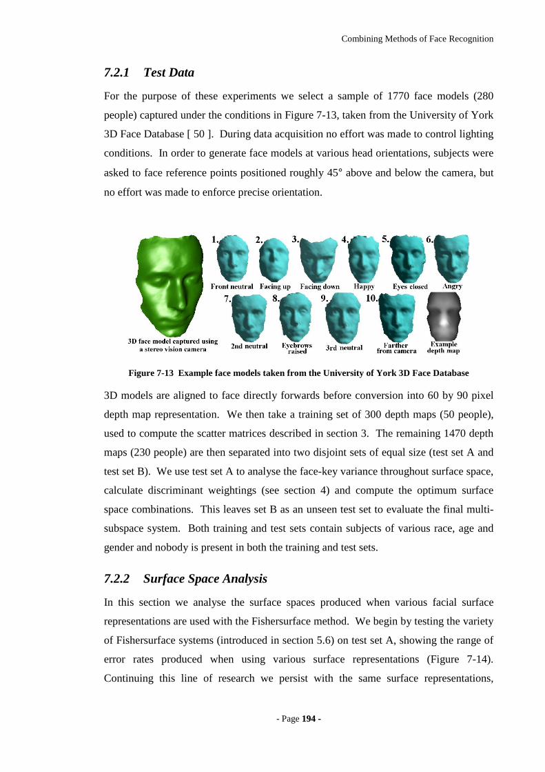
Combining Methods of Face Recognition
- Page 119944 --
7.2.1 Test Data
For the purpose of these experiments we select a sample of 1770 face models (280
people) captured under the conditions in Figure 7-13, taken from the University of York
3D Face Database [ 50 ]. During data acquisition no effort was made to control lighting
conditions. In order to generate face models at various head orientations, subjects were
asked to face reference points positioned roughly 45° above and below the camera, but
no effort was made to enforce precise orientation.
Figure 7-13 Example face models taken from the University of York 3D Face Database
3D models are aligned to face directly forwards before conversion into 60 by 90 pixel
depth map representation. We then take a training set of 300 depth maps (50 people),
used to compute the scatter matrices described in section 3. The remaining 1470 depth
maps (230 people) are then separated into two disjoint sets of equal size (test set A and
test set B). We use test set A to analyse the face-key variance throughout surface space,
calculate discriminant weightings (see section 4) and compute the optimum surface
space combinations. This leaves set B as an unseen test set to evaluate the final multi-
subspace system. Both training and test sets contain subjects of various race, age and
gender and nobody is present in both the training and test sets.
7.2.2 Surface Space Analysis
In this section we analyse the surface spaces produced when various facial surface
representations are used with the Fishersurface method. We begin by testing the variety
of Fishersurface systems (introduced in section 5.6) on test set A, showing the range of
error rates produced when using various surface representations (Figure 7-14).
Continuing this line of research we persist with the same surface representations,
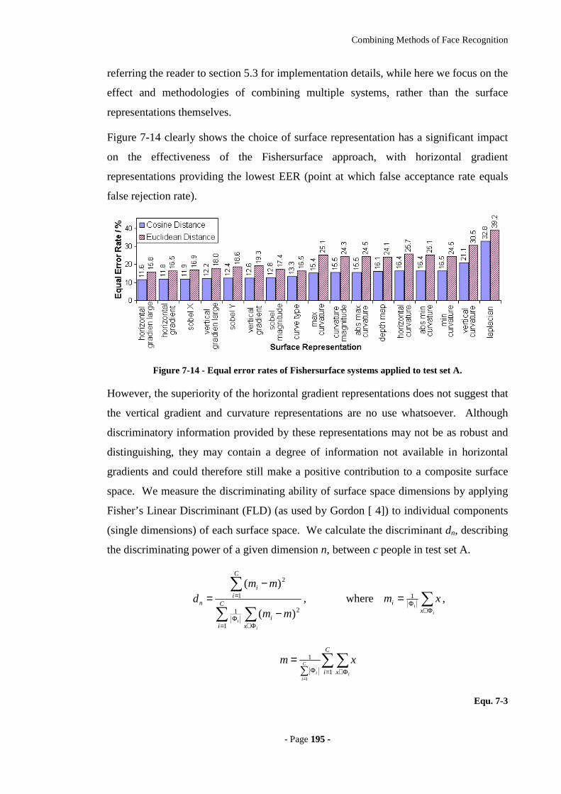
Combining Methods of Face Recognition
- Page 119955 --
referring the reader to section 5.3 for implementation details, while here we focus on the
effect and methodologies of combining multiple systems, rather than the surface
representations themselves.
Figure 7-14 clearly shows the choice of surface representation has a significant impact
on the effectiveness of the Fishersurface approach, with horizontal gradient
representations providing the lowest EER (point at which false acceptance rate equals
false rejection rate).
Figure 7-14 - Equal error rates of Fishersurface systems applied to test set A.
However, the superiority of the horizontal gradient representations does not suggest that
the vertical gradient and curvature representations are no use whatsoever. Although
discriminatory information provided by these representations may not be as robust and
distinguishing, they may contain a degree of information not available in horizontal
gradients and could therefore still make a positive contribution to a composite surface
space. We measure the discriminating ability of surface space dimensions by applying
Fisher’s Linear Discriminant (FLD) (as used by Gordon [ 4]) to individual components
(single dimensions) of each surface space. We calculate the discriminant dn, describing
the discriminating power of a given dimension n, between c people in test set A.
∑ ∑
∑
= Φ∈Φ
=
−
−= C
i xi
C
ii
n
i
imm
mmd
1
21
1
2
)(
)(, where ∑
Φ∈Φ=
i
ix
i xm 1 ,
∑∑= Φ∈Φ∑
==
C
i x i
C
ii
xm1
1
1
Equ. 7-3
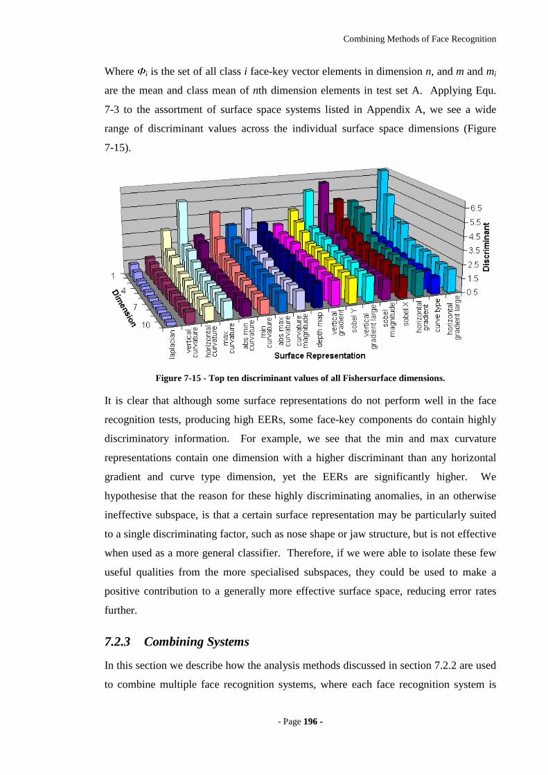
Combining Methods of Face Recognition
- Page 119966 --
Where i is the set of all class i face-key vector elements in dimension n, and m and mi
are the mean and class mean of nth dimension elements in test set A. Applying Equ.
7-3 to the assortment of surface space systems listed in Appendix A, we see a wide
range of discriminant values across the individual surface space dimensions (Figure
7-15).
Figure 7-15 - Top ten discriminant values of all Fishersurface dimensions.
It is clear that although some surface representations do not perform well in the face
recognition tests, producing high EERs, some face-key components do contain highly
discriminatory information. For example, we see that the min and max curvature
representations contain one dimension with a higher discriminant than any horizontal
gradient and curve type dimension, yet the EERs are significantly higher. We
hypothesise that the reason for these highly discriminating anomalies, in an otherwise
ineffective subspace, is that a certain surface representation may be particularly suited
to a single discriminating factor, such as nose shape or jaw structure, but is not effective
when used as a more general classifier. Therefore, if we were able to isolate these few
useful qualities from the more specialised subspaces, they could be used to make a
positive contribution to a generally more effective surface space, reducing error rates
further.
7.2.3 Combining Systems
In this section we describe how the analysis methods discussed in section 7.2.2 are used
to combine multiple face recognition systems, where each face recognition system is
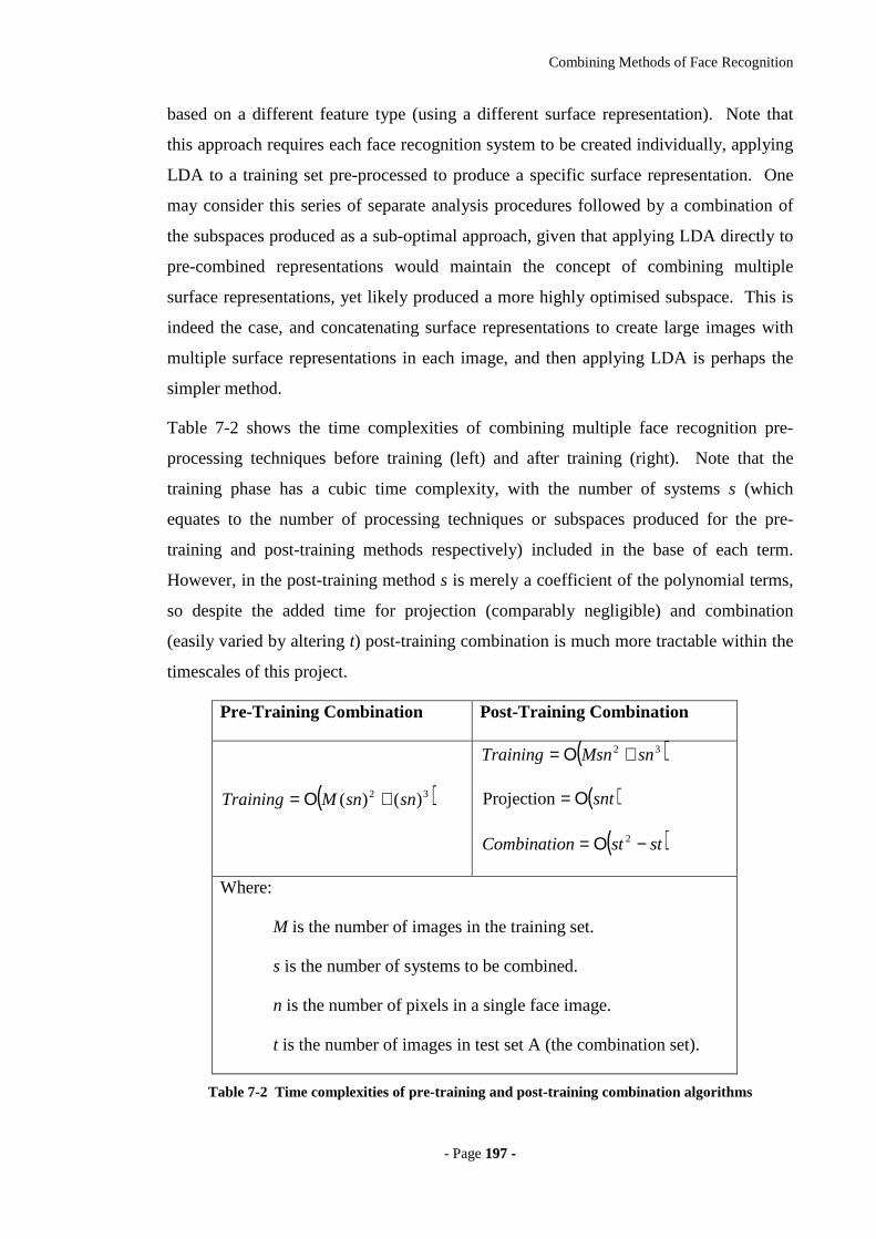
Combining Methods of Face Recognition
- Page 119977 --
based on a different feature type (using a different surface representation). Note that
this approach requires each face recognition system to be created individually, applying
LDA to a training set pre-processed to produce a specific surface representation. One
may consider this series of separate analysis procedures followed by a combination of
the subspaces produced as a sub-optimal approach, given that applying LDA directly to
pre-combined representations would maintain the concept of combining multiple
surface representations, yet likely produced a more highly optimised subspace. This is
indeed the case, and concatenating surface representations to create large images with
multiple surface representations in each image, and then applying LDA is perhaps the
simpler method.
Table 7-2 shows the time complexities of combining multiple face recognition pre-
processing techniques before training (left) and after training (right). Note that the
training phase has a cubic time complexity, with the number of systems s (which
equates to the number of processing techniques or subspaces produced for the pre-
training and post-training methods respectively) included in the base of each term.
However, in the post-training method s is merely a coefficient of the polynomial terms,
so despite the added time for projection (comparably negligible) and combination
(easily varied by altering t) post-training combination is much more tractable within the
timescales of this project.
Pre-Training Combination Post-Training Combination
( )32 )()( snsnMTraining +Ο=
( )32 snMsnTraining +Ο=
( )sntΟ=Projection
( )ststnCombinatio −Ο= 2
Where:
M is the number of images in the training set.
s is the number of systems to be combined.
n is the number of pixels in a single face image.
t is the number of images in test set A (the combination set).
Table 7-2 Time complexities of pre-training and post-training combination algorithms
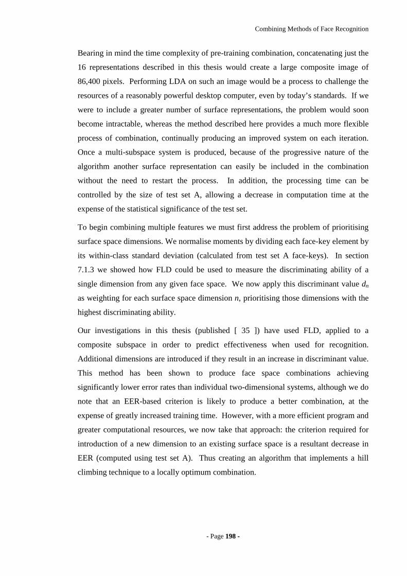
Combining Methods of Face Recognition
- Page 119988 --
Bearing in mind the time complexity of pre-training combination, concatenating just the
16 representations described in this thesis would create a large composite image of
86,400 pixels. Performing LDA on such an image would be a process to challenge the
resources of a reasonably powerful desktop computer, even by today’s standards. If we
were to include a greater number of surface representations, the problem would soon
become intractable, whereas the method described here provides a much more flexible
process of combination, continually producing an improved system on each iteration.
Once a multi-subspace system is produced, because of the progressive nature of the
algorithm another surface representation can easily be included in the combination
without the need to restart the process. In addition, the processing time can be
controlled by the size of test set A, allowing a decrease in computation time at the
expense of the statistical significance of the test set.
To begin combining multiple features we must first address the problem of prioritising
surface space dimensions. We normalise moments by dividing each face-key element by
its within-class standard deviation (calculated from test set A face-keys). In section
7.1.3 we showed how FLD could be used to measure the discriminating ability of a
single dimension from any given face space. We now apply this discriminant value dn
as weighting for each surface space dimension n, prioritising those dimensions with the
highest discriminating ability.
Our investigations in this thesis (published [ 35 ]) have used FLD, applied to a
composite subspace in order to predict effectiveness when used for recognition.
Additional dimensions are introduced if they result in an increase in discriminant value.
This method has been shown to produce face space combinations achieving
significantly lower error rates than individual two-dimensional systems, although we do
note that an EER-based criterion is likely to produce a better combination, at the
expense of greatly increased training time. However, with a more efficient program and
greater computational resources, we now take that approach: the criterion required for
introduction of a new dimension to an existing surface space is a resultant decrease in
EER (computed using test set A). Thus creating an algorithm that implements a hill
climbing technique to a locally optimum combination.

Combining Methods of Face Recognition
- Page 119999 --
Composite surface space = first dimension of best current system
Compute EER of composite surface space
For each surface representation system:
For each dimension of surface space:
Concatenate dimension onto composite surface space
Compute EER of composite surface space
If EER has not decreased:
Remove dimension from composite surface space
Save composite subspace ready for evaluation
Figure 7-16 Face space combination by dimensional accumulation algorithm, using the EER as a
fitness criteria
7.2.4 The Test Procedure
In order to evaluate the effectiveness of a surface space, we project and compare each
facial surface with every other surface in the test set, no surface is compared with itself
and each pair is compared only once. The false acceptance rate (FAR) and false
rejection rate (FRR) are then calculated as the percentage of incorrect acceptances and
incorrect rejections after applying a threshold. By varying the threshold, we produce a
series of FAR FRR pairs, which plotted on a graph produce an error curve as seen in
Figure 7-19. The equal error rate (EER, the point at which FAR equals FRR) can then
be taken as a single comparative value.
Using this test format we consider three separate data sets. The training set (τ) is used
solely to compute the scatter matrices and ultimately the projection matrix that defines
our surface subspace. The remaining data is separated into two disjoint test sets A and
B. Test set A is used to compute a FAR and FRR curves for each iteration of the
combination algorithm described above. The EER extracted from these graphs is then
used as the decision criterion as to whether a dimension is utilised or discarded. The
final test set B is used once the final combination has been computed, to provide a FAR,
FRR curve calculated using previously unseen test data.
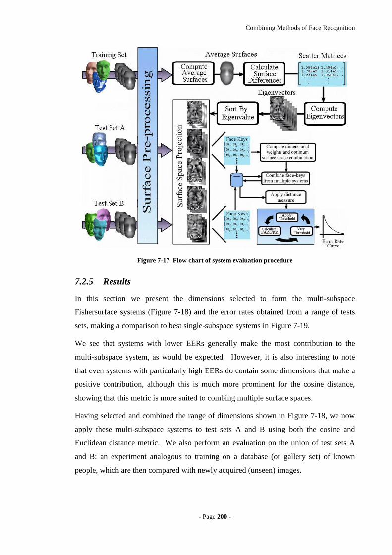
Combining Methods of Face Recognition
- Page 220000 --
Figure 7-17 Flow chart of system evaluation procedure
7.2.5 Results
In this section we present the dimensions selected to form the multi-subspace
Fishersurface systems (Figure 7-18) and the error rates obtained from a range of tests
sets, making a comparison to best single-subspace systems in Figure 7-19.
We see that systems with lower EERs generally make the most contribution to the
multi-subspace system, as would be expected. However, it is also interesting to note
that even systems with particularly high EERs do contain some dimensions that make a
positive contribution, although this is much more prominent for the cosine distance,
showing that this metric is more suited to combing multiple surface spaces.
Having selected and combined the range of dimensions shown in Figure 7-18, we now
apply these multi-subspace systems to test sets A and B using both the cosine and
Euclidean distance metric. We also perform an evaluation on the union of test sets A
and B: an experiment analogous to training on a database (or gallery set) of known
people, which are then compared with newly acquired (unseen) images.
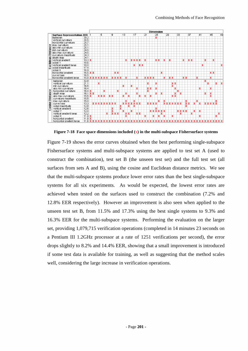
Combining Methods of Face Recognition
- Page 220011 --
Figure 7-18 Face space dimensions included (x) in the multi-subspace Fishersurface systems
Figure 7-19 shows the error curves obtained when the best performing single-subspace
Fishersurface systems and multi-subspace systems are applied to test set A (used to
construct the combination), test set B (the unseen test set) and the full test set (all
surfaces from sets A and B), using the cosine and Euclidean distance metrics. We see
that the multi-subspace systems produce lower error rates than the best single-subspace
systems for all six experiments. As would be expected, the lowest error rates are
achieved when tested on the surfaces used to construct the combination (7.2% and
12.8% EER respectively). However an improvement is also seen when applied to the
unseen test set B, from 11.5% and 17.3% using the best single systems to 9.3% and
16.3% EER for the multi-subspace systems. Performing the evaluation on the larger
set, providing 1,079,715 verification operations (completed in 14 minutes 23 seconds on
a Pentium III 1.2GHz processor at a rate of 1251 verifications per second), the error
drops slightly to 8.2% and 14.4% EER, showing that a small improvement is introduced
if some test data is available for training, as well as suggesting that the method scales
well, considering the large increase in verification operations.
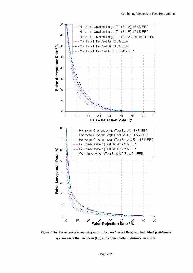
Combining Methods of Face Recognition
- Page 220022 --
Figure 7-19 Error curves comparing multi-subspace (dashed lines) and individual (solid lines)
systems using the Euclidean (top) and cosine (bottom) distance measures.
Combining Methods of Face Recognition
- Page 220033 --
7.2.6 Conclusion
We have shown how a well-known method of two-dimensional face recognition,
namely the Fisherface method, can be applied to 3D face models achieving reasonably
low error rates, depending on the surface representation used. Drawing on previous
investigations (section 7.1) combining face recognition eigenspaces [ 35 ], we have
applied the same principle to multiple 3D face recognition systems, showing that the
combination method is applicable to both two-dimensional and 3D data. Using FLD as
an analysis tool, we have confirmed the hypothesis that although some surface
representations may not perform well when used for recognition, they may harbour
highly discriminatory components that could complement other surface spaces.
Iteratively improving error rates on a small test set, we have built up a combination of
dimensions extracted from a variety of surface spaces, each utilising a different surface
representation. This method of combination has been shown to be most effective when
used with the cosine distance metric, in which a selection of 184 dimensions were
combined from 16 of the 17 surface spaces, reducing the EER from 11.6% to 8.2%.
Applying the same composite surface space to an unseen test set of data presenting
typical difficulties when performing recognition, we have demonstrated a similar
reduction in error from 11.5% to 9.3% EER.
Evaluating the multi-subspace system at its fundamental level, using 1,079,715
verification operations between 3D facial surfaces, demonstrates that combining
multiple surface space dimensions improves effectiveness of the core recognition
algorithm. Error rates have been significantly reduced to state-of-the-art levels, when
evaluated on a difficult test set including variations in expression and orientation.
However, we have not applied any additional heuristics, typically incorporated into
fully functional commercial and industrial systems. For example, we have not
experimented with multiple facial alignments, optimising crop regions or storing
multiple gallery images. All of which are known to improve error rates and can easily
be applied to the multi-subspace systems presented here. With these additional
measures in place, it is likely that the improvements made to the core algorithm will
propagate through to producing a highly effective face recognition system. Given the
fast 3D capture method, small face-keys of 184 vector elements (allowing extremely

Combining Methods of Face Recognition
- Page 220044 --
fast comparisons), invariance to lighting conditions and facial orientation, this system is
particularly suited to security and surveillance applications.
Combining Methods of Face Recognition
- Page 220055 --
77..33 MM eetthhooddss ooff CCoommbbiinnaatt iioonn OOpptt iimmiissaatt iioonn
In the previous section we discussed two methods of selecting a set of dimensions from
the complete collection of available face space and surface space systems and
combining them to produce a augmented feature space that produces lower error rates
than any of the individual systems alone. Some brief analysis and experimentation
demonstrates that although the global discriminant value can be used as a fast
approximation of system effectiveness, performing a complete evaluation and
subsequently using the EER as the selection criteria is a significantly more effective
selection criterion for the combination algorithm. Another aspect of the combination
algorithm, which we have not yet addressed, is the order in which each dimension is
selected and tested. Initial experimentation has indicated that this may be important, as
the value of contribution of any candidate dimension is dependant on those dimensions
already included in the existing composite subspace i.e. the optimisation is local, not
global.
Actually, we have already begun to touch upon this issue, although somewhat
indirectly, in the combination methods already discussed: it is precisely the reason we
begin our combination with all dimensions from the current best performing system.
Consider the case in which our composite face space consists of a single dimension,
selected by chance from the worst of the face space systems. The next dimension tested
for incorporation is almost certain to succeed (regardless of how discriminating it is), as
such few features are currently utilised and even the smallest amount of additional
discriminatory information would improve the system. On the other hand, once a
combination incorporates a large number of dimensions is becomes increasingly
unlikely that the next dimension will be of any benefit. These effects are witnessed in
that more dimensions nearer the start of the list are included than those towards the end,
as can be seen in section 7.1.6 and 7.2.5 (in which face space systems were considered
for combination in order of ascending EER).
Some additional experimentation has uncovered another phenomenon that we must also
consider here. It is possible that the incorporation of numerous dimensions into an
existing subspace will significantly improve results; yet incorporating any one of those
same dimensions individually can actually increase error rates. The combination
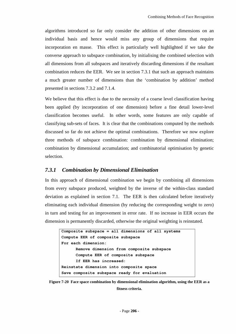
Combining Methods of Face Recognition
- Page 220066 --
algorithms introduced so far only consider the addition of other dimensions on an
individual basis and hence would miss any group of dimensions that require
incorporation en masse. This effect is particularly well highlighted if we take the
converse approach to subspace combination, by initialising the combined selection with
all dimensions from all subspaces and iteratively discarding dimensions if the resultant
combination reduces the EER. We see in section 7.3.1 that such an approach maintains
a much greater number of dimensions than the ‘combination by addition’ method
presented in sections 7.3.2 and 7.1.4.
We believe that this effect is due to the necessity of a coarse level classification having
been applied (by incorporation of one dimension) before a fine detail lower-level
classification becomes useful. In other words, some features are only capable of
classifying sub-sets of faces. It is clear that the combinations computed by the methods
discussed so far do not achieve the optimal combinations. Therefore we now explore
three methods of subspace combination: combination by dimensional elimination;
combination by dimensional accumulation; and combinatorial optimisation by genetic
selection.
7.3.1 Combination by Dimensional Elimination
In this approach of dimensional combination we begin by combining all dimensions
from every subspace produced, weighted by the inverse of the within-class standard
deviation as explained in section 7.1. The EER is then calculated before iteratively
eliminating each individual dimension (by reducing the corresponding weight to zero)
in turn and testing for an improvement in error rate. If no increase in EER occurs the
dimension is permanently discarded, otherwise the original weighting is reinstated.
Composite subspace = all dimensions of all systems
Compute EER of composite subspace
For each dimension:
Remove dimension from composite subspace
Compute EER of composite subspace
If EER has increased:
Reinstate dimension into composite space
Save composite subspace ready for evaluation
Figure 7-20 Face space combination by dimensional elimination algorithm, using the EER as a
fitness criteria.
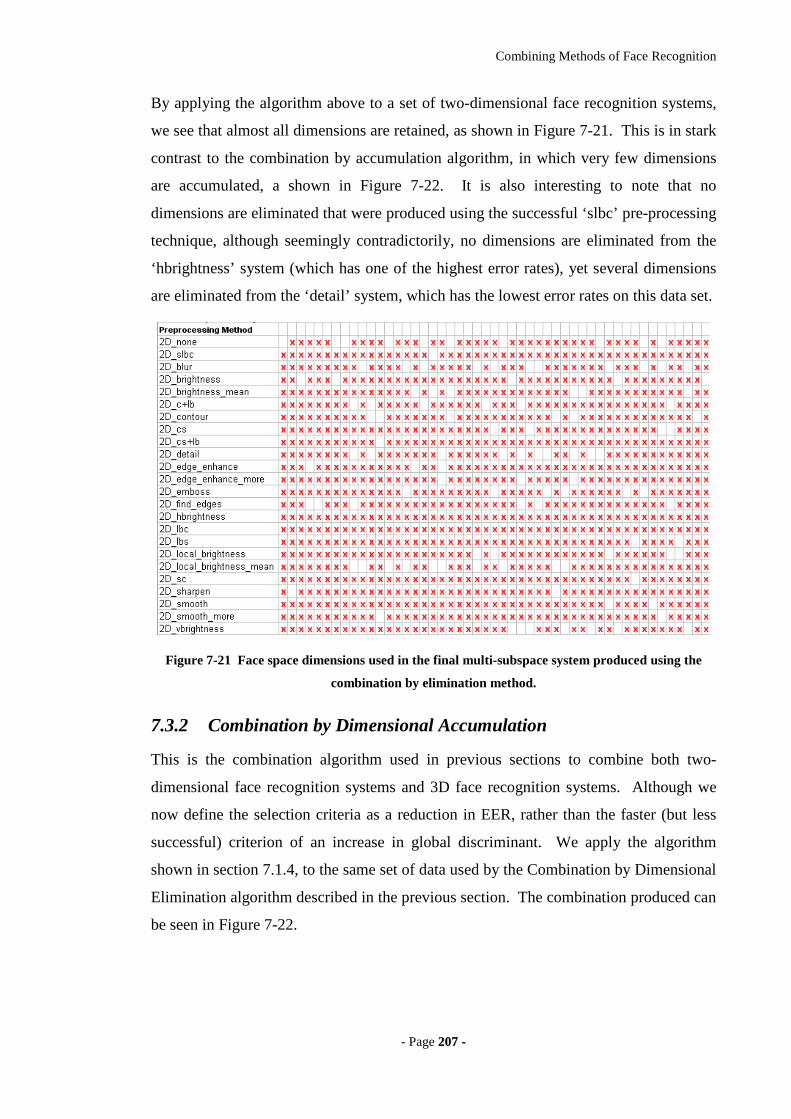
Combining Methods of Face Recognition
- Page 220077 --
By applying the algorithm above to a set of two-dimensional face recognition systems,
we see that almost all dimensions are retained, as shown in Figure 7-21. This is in stark
contrast to the combination by accumulation algorithm, in which very few dimensions
are accumulated, a shown in Figure 7-22. It is also interesting to note that no
dimensions are eliminated that were produced using the successful ‘slbc’ pre-processing
technique, although seemingly contradictorily, no dimensions are eliminated from the
‘hbrightness’ system (which has one of the highest error rates), yet several dimensions
are eliminated from the ‘detail’ system, which has the lowest error rates on this data set.
Figure 7-21 Face space dimensions used in the final multi-subspace system produced using the
combination by elimination method.
7.3.2 Combination by Dimensional Accumulation
This is the combination algorithm used in previous sections to combine both two-
dimensional face recognition systems and 3D face recognition systems. Although we
now define the selection criteria as a reduction in EER, rather than the faster (but less
successful) criterion of an increase in global discriminant. We apply the algorithm
shown in section 7.1.4, to the same set of data used by the Combination by Dimensional
Elimination algorithm described in the previous section. The combination produced can
be seen in Figure 7-22.
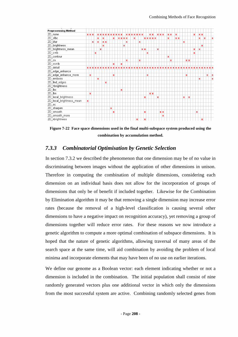
Combining Methods of Face Recognition
- Page 220088 --
Figure 7-22 Face space dimensions used in the final multi-subspace system produced using the
combination by accumulation method.
7.3.3 Combinatorial Optimisation by Genetic Selection
In section 7.3.2 we described the phenomenon that one dimension may be of no value in
discriminating between images without the application of other dimensions in unison.
Therefore in computing the combination of multiple dimensions, considering each
dimension on an individual basis does not allow for the incorporation of groups of
dimensions that only be of benefit if included together. Likewise for the Combination
by Elimination algorithm it may be that removing a single dimension may increase error
rates (because the removal of a high-level classification is causing several other
dimensions to have a negative impact on recognition accuracy), yet removing a group of
dimensions together will reduce error rates. For these reasons we now introduce a
genetic algorithm to compute a more optimal combination of subspace dimensions. It is
hoped that the nature of genetic algorithms, allowing traversal of many areas of the
search space at the same time, will aid combination by avoiding the problem of local
minima and incorporate elements that may have been of no use on earlier iterations.
We define our genome as a Boolean vector: each element indicating whether or not a
dimension is included in the combination. The initial population shall consist of nine
randomly generated vectors plus one additional vector in which only the dimensions
from the most successful system are active. Combining randomly selected genes from
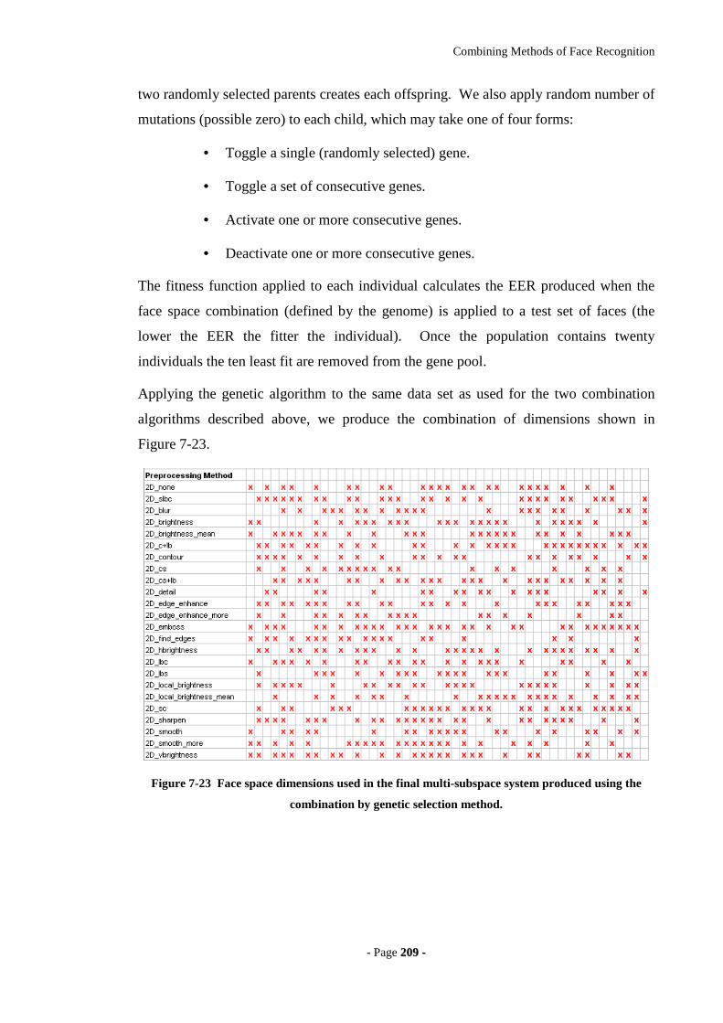
Combining Methods of Face Recognition
- Page 220099 --
two randomly selected parents creates each offspring. We also apply random number of
mutations (possible zero) to each child, which may take one of four forms:
• Toggle a single (randomly selected) gene.
• Toggle a set of consecutive genes.
• Activate one or more consecutive genes.
• Deactivate one or more consecutive genes.
The fitness function applied to each individual calculates the EER produced when the
face space combination (defined by the genome) is applied to a test set of faces (the
lower the EER the fitter the individual). Once the population contains twenty
individuals the ten least fit are removed from the gene pool.
Applying the genetic algorithm to the same data set as used for the two combination
algorithms described above, we produce the combination of dimensions shown in
Figure 7-23.
Figure 7-23 Face space dimensions used in the final multi-subspace system produced using the
combination by genetic selection method.
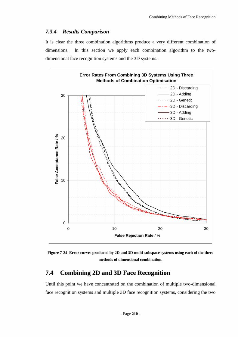
Combining Methods of Face Recognition
- Page 221100 --
7.3.4 Results Comparison
It is clear the three combination algorithms produce a very different combination of
dimensions. In this section we apply each combination algorithm to the two-
dimensional face recognition systems and the 3D systems.
Error Rates From Combining 3D Systems Using Three Methods of Combination Optimisation
0
10
20
30
0 10 20 30
False Rejection Rate / %
Fal
se A
ccep
tan
ce R
ate
/ %
2D - Discarding
2D - Adding
2D - Genetic
3D - Discarding
3D - Adding
3D - Genetic
Figure 7-24 Error curves produced by 2D and 3D multi-subspace systems using each of the three
methods of dimensional combination.
77..44 CCoommbbiinniinngg 22DD aanndd 33DD FFaaccee RReeccooggnnii tt iioonn
Until this point we have concentrated on the combination of multiple two-dimensional
face recognition systems and multiple 3D face recognition systems, considering the two
Combining Methods of Face Recognition
- Page 221111 --
data types separately in the hope that different representations of the same data may
encapsulation different features, which can subsequently be combined to improve
recognition accuracy. We now extend this approach to combine 3D systems with two-
dimensional systems in order to take advantage of both the geometrical shape available
from 3D face models as well as the colour and texture information provided by two-
dimensional images. It is likely that such a system will produce reductions in error
rates, as it is probable that many features of the two types of data are mutually exclusive
and therefore combine to great benefit. The combination of these two types of data is
viable as the 3D camera used to create 3D face models is capable of capturing both 3D
shape data and two-dimensional texture images simultaneously. Therefore, a 2D/3D
hybrid system is applicable to real world applications without the need for any
additional equipment.
There are a number of ways in which we can utilise the two-dimensional data provided
by the 3D camera. Firstly, we could simply use the standard 2D images, extract the face
and align the images according to the position of the eyes, as with the two-dimensional
systems already described in section 4. However, as the 3D face models produced are
texture mapped with the 2D images another possibility presents itself. We have
previously discussed the possibility of matching two-dimensional projections of a
texture mapped 3D model in section 6.1. This approach effectively allows standard
two-dimensional recognition methods to gain the advantage of 3D orientation
normalisation and hence expand the range of facial orientations that can be recognised.
We therefore have three paradigms of data that may be combined into a unified system:
3D depth maps, 2D images and 2D projections.
7.4.1 Results
In this section we present the error rates produced when two-dimensional and 3D face
recognition systems are combined and tested on the same data set as described in 7.3
(test set B). We apply the three combination algorithms to all pre-processing techniques
and surface representations using test set A as the combination analysis data, before
computing the error curve using test set B.
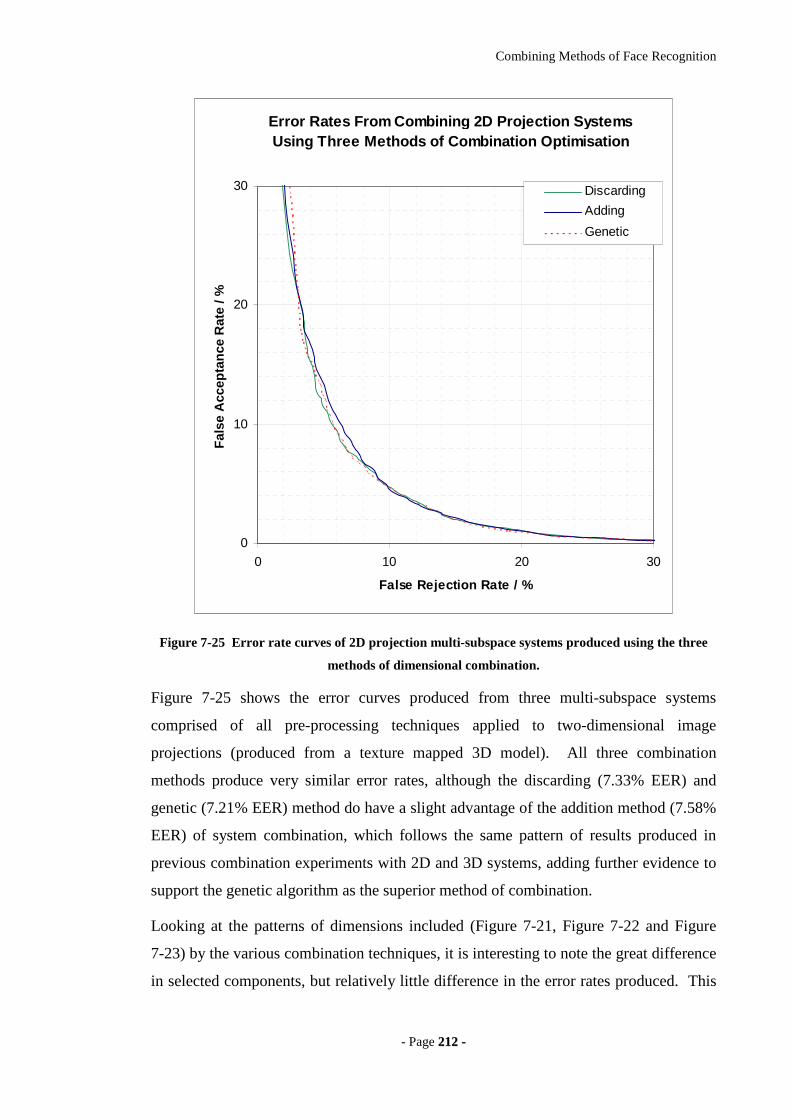
Combining Methods of Face Recognition
- Page 221122 --
Error Rates From Combining 2D Projection Systems Using Three Methods of Combination Optimisation
0
10
20
30
0 10 20 30
False Rejection Rate / %
Fal
se A
ccep
tan
ce R
ate
/ %
Discarding
Adding
Genetic
Figure 7-25 Error rate curves of 2D projection multi-subspace systems produced using the three
methods of dimensional combination.
Figure 7-25 shows the error curves produced from three multi-subspace systems
comprised of all pre-processing techniques applied to two-dimensional image
projections (produced from a texture mapped 3D model). All three combination
methods produce very similar error rates, although the discarding (7.33% EER) and
genetic (7.21% EER) method do have a slight advantage of the addition method (7.58%
EER) of system combination, which follows the same pattern of results produced in
previous combination experiments with 2D and 3D systems, adding further evidence to
support the genetic algorithm as the superior method of combination.
Looking at the patterns of dimensions included (Figure 7-21, Figure 7-22 and Figure
7-23) by the various combination techniques, it is interesting to note the great difference
in selected components, but relatively little difference in the error rates produced. This

Combining Methods of Face Recognition
- Page 221133 --
suggests that the fitness function of the combination search space has many peaks of
similar magnitude, scattered throughout the search space. This makes it particularly
difficult to find the optimum without a global search (unfeasible at current processing
speeds).
In Figure 7-26 we have continued this line of investigation to combine 3D data (using
the various surface representations discussed in section 5.3) and the projected 2D
texture image. Therefore, we utilise both the geometric shape data, as well as the
orientation normalised two-dimensional texture information in a single system. Again
we test all three methods of combination.
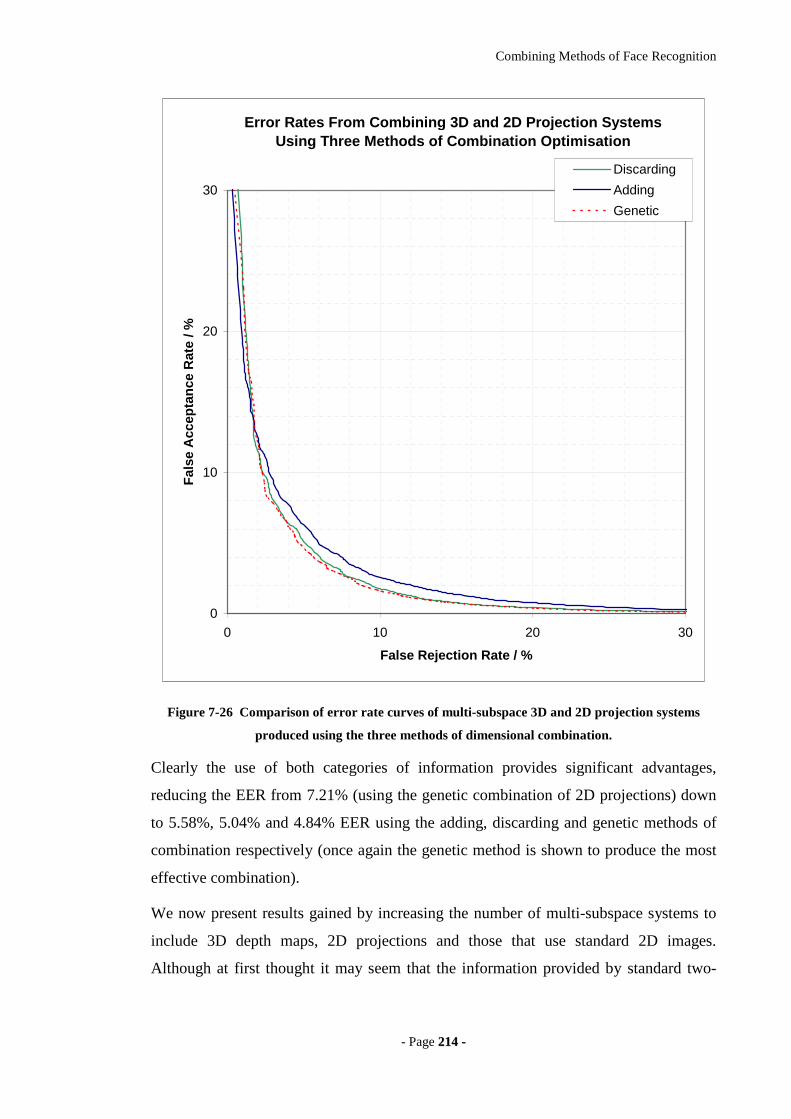
Combining Methods of Face Recognition
- Page 221144 --
Error Rates From Combining 3D and 2D Projection Systems Using Three Methods of Combination Optimisation
0
10
20
30
0 10 20 30
False Rejection Rate / %
Fal
se A
ccep
tan
ce R
ate
/ %Discarding
Adding
Genetic
Figure 7-26 Comparison of error rate curves of multi-subspace 3D and 2D projection systems
produced using the three methods of dimensional combination.
Clearly the use of both categories of information provides significant advantages,
reducing the EER from 7.21% (using the genetic combination of 2D projections) down
to 5.58%, 5.04% and 4.84% EER using the adding, discarding and genetic methods of
combination respectively (once again the genetic method is shown to produce the most
effective combination).
We now present results gained by increasing the number of multi-subspace systems to
include 3D depth maps, 2D projections and those that use standard 2D images.
Although at first thought it may seem that the information provided by standard two-
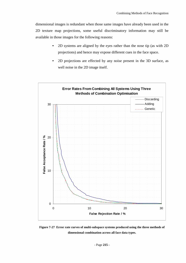
Combining Methods of Face Recognition
- Page 221155 --
dimensional images is redundant when those same images have already been used in the
2D texture map projections, some useful discriminatory information may still be
available in those images for the following reasons:
• 2D systems are aligned by the eyes rather than the nose tip (as with 2D
projections) and hence may expose different cues in the face space.
• 2D projections are effected by any noise present in the 3D surface, as
well noise in the 2D image itself.
Error Rates From Combining All Systems Using Three Methods of Combination Optimisation
0
10
20
30
0 10 20 30
False Rejection Rate / %
Fal
se A
ccep
tan
ce R
ate
/ %
Discarding
Adding
Genetic
Figure 7-27 Error rate curves of multi-subspace systems produced using the three methods of
dimensional combination across all face data types.
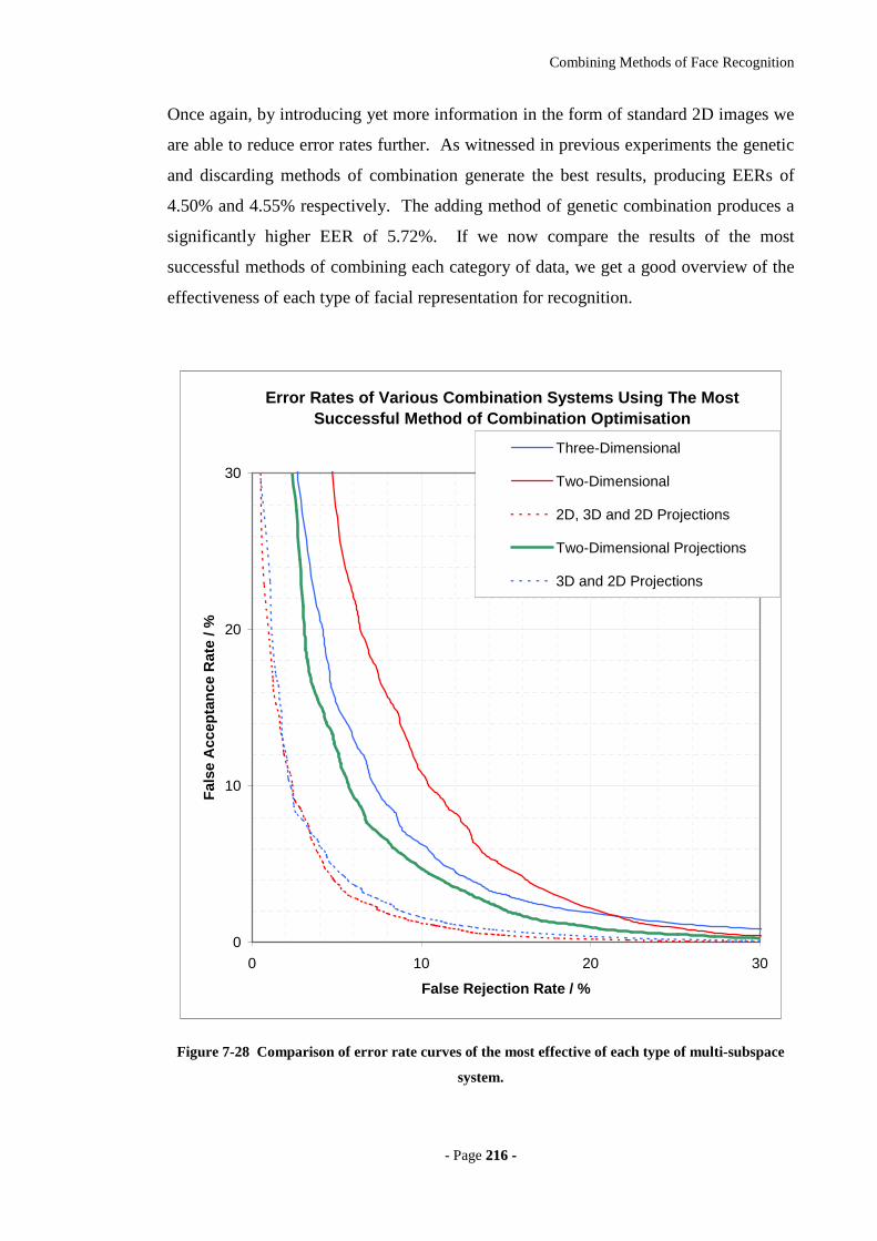
Combining Methods of Face Recognition
- Page 221166 --
Once again, by introducing yet more information in the form of standard 2D images we
are able to reduce error rates further. As witnessed in previous experiments the genetic
and discarding methods of combination generate the best results, producing EERs of
4.50% and 4.55% respectively. The adding method of genetic combination produces a
significantly higher EER of 5.72%. If we now compare the results of the most
successful methods of combining each category of data, we get a good overview of the
effectiveness of each type of facial representation for recognition.
Error Rates of Various Combination Systems Using The Most Successful Method of Combination Optimisation
0
10
20
30
0 10 20 30
False Rejection Rate / %
Fal
se A
ccep
tan
ce R
ate
/ %
Three-Dimensional
Two-Dimensional
2D, 3D and 2D Projections
Two-Dimensional Projections
3D and 2D Projections
Figure 7-28 Comparison of error rate curves of the most effective of each type of multi-subspace
system.
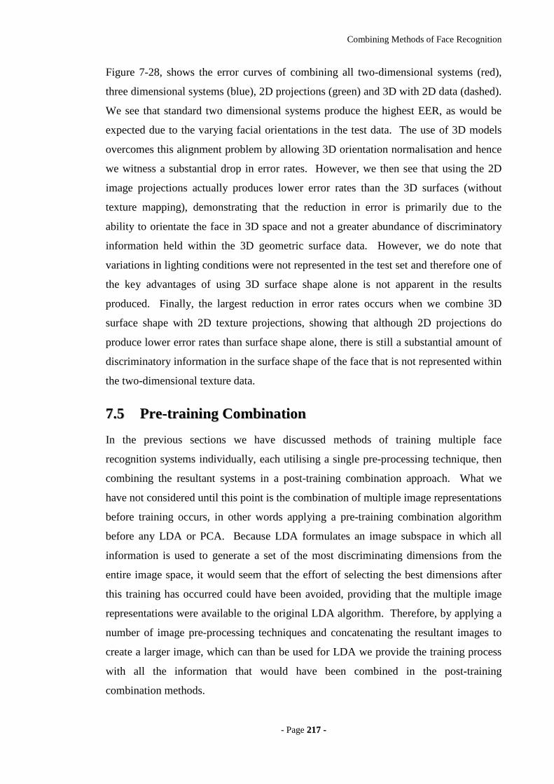
Combining Methods of Face Recognition
- Page 221177 --
Figure 7-28, shows the error curves of combining all two-dimensional systems (red),
three dimensional systems (blue), 2D projections (green) and 3D with 2D data (dashed).
We see that standard two dimensional systems produce the highest EER, as would be
expected due to the varying facial orientations in the test data. The use of 3D models
overcomes this alignment problem by allowing 3D orientation normalisation and hence
we witness a substantial drop in error rates. However, we then see that using the 2D
image projections actually produces lower error rates than the 3D surfaces (without
texture mapping), demonstrating that the reduction in error is primarily due to the
ability to orientate the face in 3D space and not a greater abundance of discriminatory
information held within the 3D geometric surface data. However, we do note that
variations in lighting conditions were not represented in the test set and therefore one of
the key advantages of using 3D surface shape alone is not apparent in the results
produced. Finally, the largest reduction in error rates occurs when we combine 3D
surface shape with 2D texture projections, showing that although 2D projections do
produce lower error rates than surface shape alone, there is still a substantial amount of
discriminatory information in the surface shape of the face that is not represented within
the two-dimensional texture data.
77..55 PPrr ee--tt rr aaiinniinngg CCoommbbiinnaatt iioonn
In the previous sections we have discussed methods of training multiple face
recognition systems individually, each utilising a single pre-processing technique, then
combining the resultant systems in a post-training combination approach. What we
have not considered until this point is the combination of multiple image representations
before training occurs, in other words applying a pre-training combination algorithm
before any LDA or PCA. Because LDA formulates an image subspace in which all
information is used to generate a set of the most discriminating dimensions from the
entire image space, it would seem that the effort of selecting the best dimensions after
this training has occurred could have been avoided, providing that the multiple image
representations were available to the original LDA algorithm. Therefore, by applying a
number of image pre-processing techniques and concatenating the resultant images to
create a larger image, which can than be used for LDA we provide the training process
with all the information that would have been combined in the post-training
combination methods.
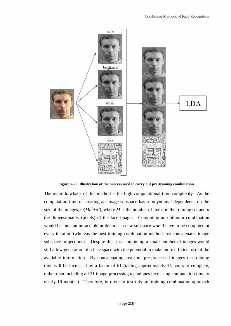
Combining Methods of Face Recognition
- Page 221188 --
Figure 7-29 Illustration of the process used to carry out pre-training combination.
The main drawback of this method is the high computational time complexity. As the
computation time of creating an image subspace has a polynomial dependence on the
size of the images, O(Mn2+n3), where M is the number of items in the training set and n
the dimensionality (pixels) of the face images. Computing an optimum combination
would become an intractable problem as a new subspace would have to be computed at
every iteration (whereas the post-training combination method just concatenates image
subspace projections). Despite this, just combining a small number of images would
still allow generation of a face space with the potential to make more efficient use of the
available information. By concatenating just four pre-processed images the training
time will be increased by a factor of 61 (taking approximately 15 hours to complete,
rather than including all 31 image-processing techniques increasing computation time to
nearly 10 months). Therefore, in order to test this pre-training combination approach
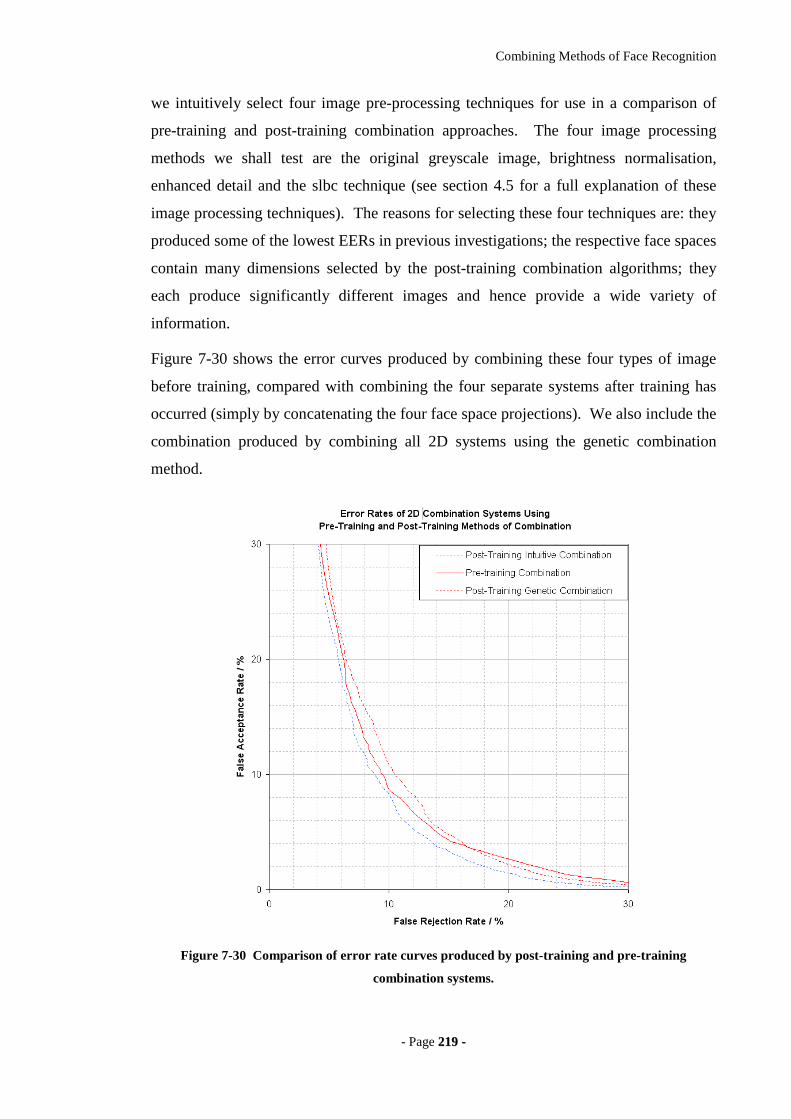
Combining Methods of Face Recognition
- Page 221199 --
we intuitively select four image pre-processing techniques for use in a comparison of
pre-training and post-training combination approaches. The four image processing
methods we shall test are the original greyscale image, brightness normalisation,
enhanced detail and the slbc technique (see section 4.5 for a full explanation of these
image processing techniques). The reasons for selecting these four techniques are: they
produced some of the lowest EERs in previous investigations; the respective face spaces
contain many dimensions selected by the post-training combination algorithms; they
each produce significantly different images and hence provide a wide variety of
information.
Figure 7-30 shows the error curves produced by combining these four types of image
before training, compared with combining the four separate systems after training has
occurred (simply by concatenating the four face space projections). We also include the
combination produced by combining all 2D systems using the genetic combination
method.
Figure 7-30 Comparison of error rate curves produced by post-training and pre-training
combination systems.
Combining Methods of Face Recognition
- Page 222200 --
This experiment has produced some interesting results. Firstly, we see that the
combination computed by the genetic combination algorithm is not optimal. Even
though the genetic combination contains various dimensions from all twenty-four 2D
systems (10.33% EER), a simple intuitive selection of just four systems produces a
lower EER of 9.26%, suggesting that the evolution methods used in the genetic
algorithm could be improved by toggling all dimensions from a entire face space in a
single mutation. More surprisingly we see that the error rates produced by combining
the four systems before training are higher (with an EER of 9.66%) than those produced
by combining the four systems after training. There are a number of possible reasons
for this outcome:
• The two-stage training process of the post-training combination method
acts as a filtering mechanism for any features that have been over-trained
on the test data, whereas any such features will remain in the pre-training
combination method.
• By concatenating four images before applying LDA we have supplied
significantly more data, much of which is simply a different
representation of the same (possibly biased) information, giving extra
weight to what may actually be poor features for discrimination if
applied to a different set of data.
• Because each image is derived from the same original image it may be
that the noise to signal ratio is substantially increased through
concatenation, leading to a relatively poor subspace. However, by
performing LDA on the individual smaller images with a better signal to
noise ratio, several more effective subspaces are produced.
• It is well known that PCA and LDA methods ideally need a collection of
training images similar in quantity to the dimensionality of the data for a
statistically significant analysis. This is typically not the case with face
recognition systems, worsened by increasing the image size by a factor
of four.
• The combination process accumulates dimensions based on the same
criteria used to evaluate performance (the EER). This combination

Combining Methods of Face Recognition
- Page 222211 --
process may therefore be more suited to producing a better subspace
(according to the evaluation criteria) than PCA and LDA, which merely
attempt to produce greatest between-class scatter. Such representations
are not necessarily optimal for classification due to subspace manifolds
and local clustering.
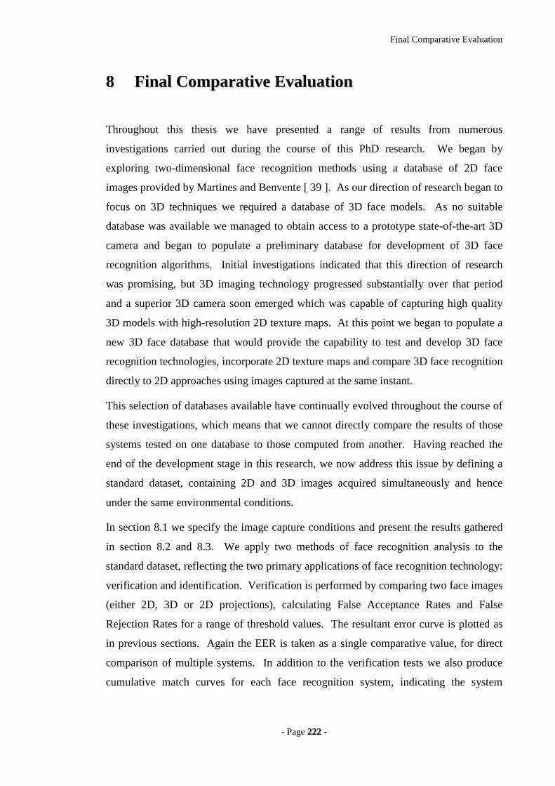
Final Comparative Evaluation
- Page 222222 --
88 FFiinnaall CCoommppaarr aatt iivvee EEvvaalluuaatt iioonn
Throughout this thesis we have presented a range of results from numerous
investigations carried out during the course of this PhD research. We began by
exploring two-dimensional face recognition methods using a database of 2D face
images provided by Martines and Benvente [ 39 ]. As our direction of research began to
focus on 3D techniques we required a database of 3D face models. As no suitable
database was available we managed to obtain access to a prototype state-of-the-art 3D
camera and began to populate a preliminary database for development of 3D face
recognition algorithms. Initial investigations indicated that this direction of research
was promising, but 3D imaging technology progressed substantially over that period
and a superior 3D camera soon emerged which was capable of capturing high quality
3D models with high-resolution 2D texture maps. At this point we began to populate a
new 3D face database that would provide the capability to test and develop 3D face
recognition technologies, incorporate 2D texture maps and compare 3D face recognition
directly to 2D approaches using images captured at the same instant.
This selection of databases available have continually evolved throughout the course of
these investigations, which means that we cannot directly compare the results of those
systems tested on one database to those computed from another. Having reached the
end of the development stage in this research, we now address this issue by defining a
standard dataset, containing 2D and 3D images acquired simultaneously and hence
under the same environmental conditions.
In section 8.1 we specify the image capture conditions and present the results gathered
in section 8.2 and 8.3. We apply two methods of face recognition analysis to the
standard dataset, reflecting the two primary applications of face recognition technology:
verification and identification. Verification is performed by comparing two face images
(either 2D, 3D or 2D projections), calculating False Acceptance Rates and False
Rejection Rates for a range of threshold values. The resultant error curve is plotted as
in previous sections. Again the EER is taken as a single comparative value, for direct
comparison of multiple systems. In addition to the verification tests we also produce
cumulative match curves for each face recognition system, indicating the system

Final Comparative Evaluation
- Page 222233 --
effectiveness in searching a large database of facial images to identify the correct
subject.
88..11 DDaattaabbaassee SSppeeccii ff iiccaatt iioonn
For the purpose of these experiments we select a sample of 1770 faces (280 people)
captured under the conditions in Figure 8-1, taken from the University of York 3D Face
Database [ 50 ]. Each face is represented by a standard two-dimensional greyscale
bitmap image, a 3D face model and a texture map projection of the orientation
normalised 3D model (also stored as a 2D greyscale bitmap). Figure 8-1 shows the
range of capture conditions present in the database, but we refer the reader to section 5.1
for a detailed explanation of how the data was acquired and the specific data formats.
A test set of 735 faces (115 people) is selected at random to compute error rates and
cumulative match rates, leaving the remaining 1035 faces (165 people) to use in training
the various face recognition systems. Typically, 300 of these faces are used to compute
the face space projection matrices, while the face space combination methods require
the additional faces in order to compute the best system combinations. The training and
test sets are completely disjoint, so that none of the faces (or the people) in the training
sets are present in the unseen test set.
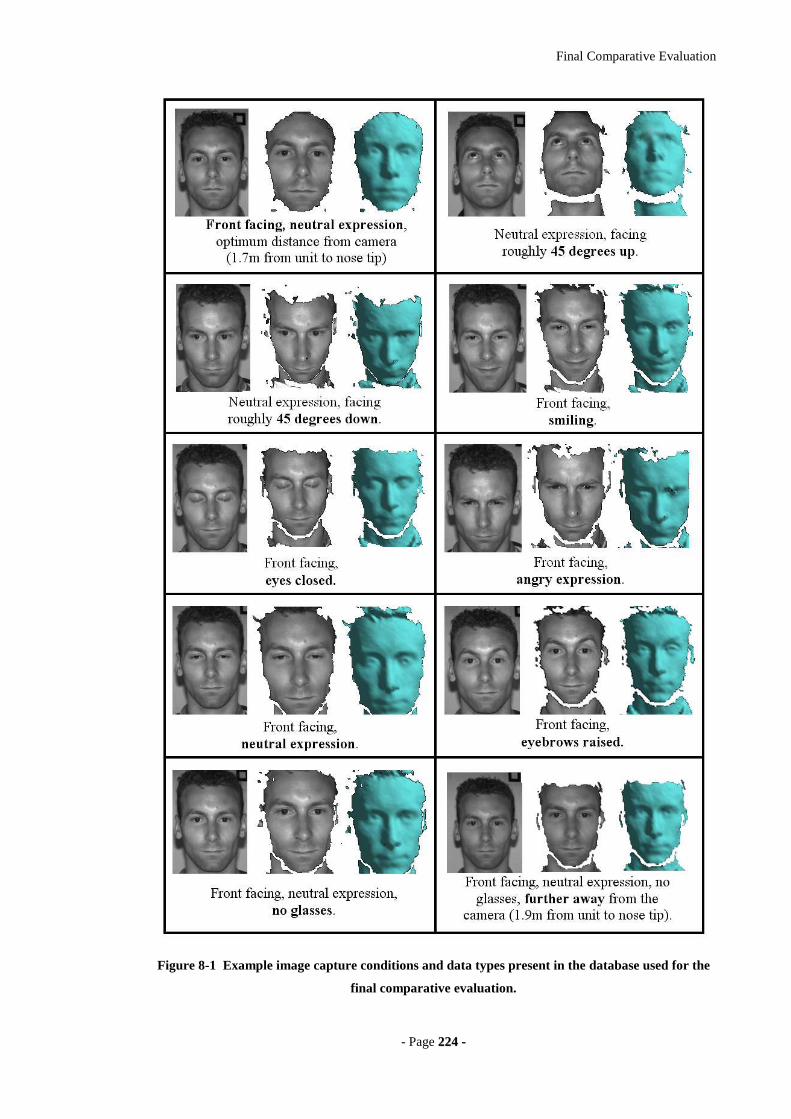
Final Comparative Evaluation
- Page 222244 --
Figure 8-1 Example image capture conditions and data types present in the database used for the
final comparative evaluation.
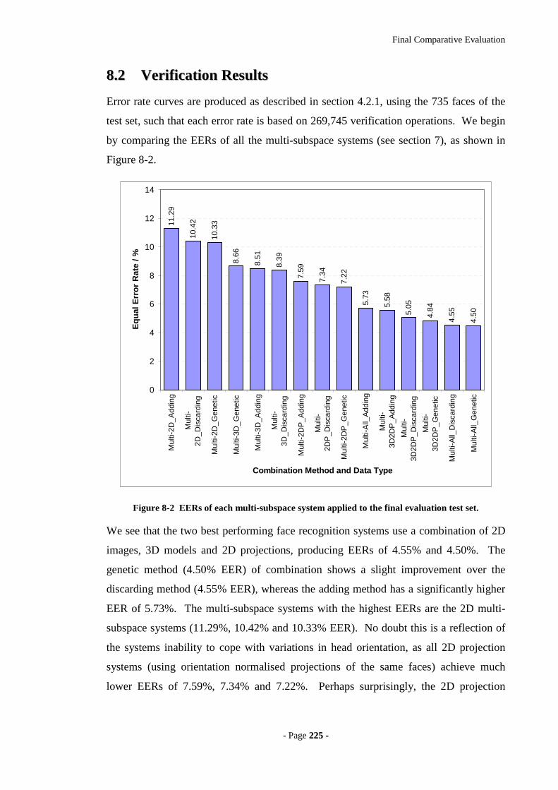
Final Comparative Evaluation
- Page 222255 --
88..22 VVeerr ii ff iiccaatt iioonn RReessuull ttss
Error rate curves are produced as described in section 4.2.1, using the 735 faces of the
test set, such that each error rate is based on 269,745 verification operations. We begin
by comparing the EERs of all the multi-subspace systems (see section 7), as shown in
Figure 8-2. 11
.29
10.4
2
10.3
3
8.66
8.51
8.39
7.59
7.34
7.22
5.73
5.58
5.05
4.84
4.55
4.50
0
2
4
6
8
10
12
14
Mul
ti-2D
_Add
ing
Mul
ti-2D
_Dis
card
ing
Mul
ti-2D
_Gen
etic
Mul
ti-3D
_Gen
etic
Mul
ti-3D
_Add
ing
Mul
ti-3D
_Dis
card
ing
Mul
ti-2D
P_A
ddin
g
Mul
ti-2D
P_D
isca
rdin
g
Mul
ti-2D
P_G
enet
ic
Mul
ti-A
ll_A
ddin
g
Mul
ti-3D
2DP
_Add
ing
Mul
ti-3D
2DP
_Dis
card
ing
Mul
ti-3D
2DP
_Gen
etic
Mul
ti-A
ll_D
isca
rdin
g
Mul
ti-A
ll_G
enet
icCombination Method and Data Type
Eq
ual
Err
or
Rat
e / %
Figure 8-2 EERs of each multi-subspace system applied to the final evaluation test set.
We see that the two best performing face recognition systems use a combination of 2D
images, 3D models and 2D projections, producing EERs of 4.55% and 4.50%. The
genetic method (4.50% EER) of combination shows a slight improvement over the
discarding method (4.55% EER), whereas the adding method has a significantly higher
EER of 5.73%. The multi-subspace systems with the highest EERs are the 2D multi-
subspace systems (11.29%, 10.42% and 10.33% EER). No doubt this is a reflection of
the systems inability to cope with variations in head orientation, as all 2D projection
systems (using orientation normalised projections of the same faces) achieve much
lower EERs of 7.59%, 7.34% and 7.22%. Perhaps surprisingly, the 2D projection
Final Comparative Evaluation
- Page 222266 --
systems outperform the systems that use 3D face models, demonstrating that the colour
and texture of the face is more discriminating than the face shape alone. However, as
variations in lighting condition were not included in the test set, we do expect to see
lower error rates from the 2D systems than if strong variations in lighting conditions
were included in the test data.
We now expand our comparison of face recognition systems to examine a greater range
of FARs and FRRs by looking at the full error curve of eight face recognition systems.
Figure 8-3 shows the best performing single-subspace 2D, 3D and 2D projection
systems, compared with the best performing multi-subspace 2D, 3D and 2D projection
systems.
Figure 8-3 Error rate curves of the most effective face recognition systems using each type of face
data and combinations of those systems.
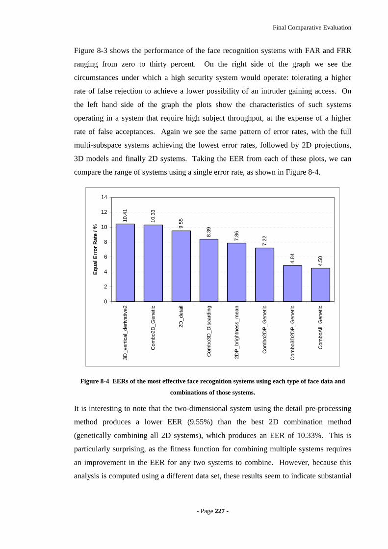
Final Comparative Evaluation
- Page 222277 --
Figure 8-3 shows the performance of the face recognition systems with FAR and FRR
ranging from zero to thirty percent. On the right side of the graph we see the
circumstances under which a high security system would operate: tolerating a higher
rate of false rejection to achieve a lower possibility of an intruder gaining access. On
the left hand side of the graph the plots show the characteristics of such systems
operating in a system that require high subject throughput, at the expense of a higher
rate of false acceptances. Again we see the same pattern of error rates, with the full
multi-subspace systems achieving the lowest error rates, followed by 2D projections,
3D models and finally 2D systems. Taking the EER from each of these plots, we can
compare the range of systems using a single error rate, as shown in Figure 8-4.
10.4
1
10.3
3
9.55
8.39
7.86
7.22
4.84
4.50
0
2
4
6
8
10
12
14
3D_v
ertic
al_d
eriv
ativ
e2
Com
bo2D
_Gen
etic
2D_d
etai
l
Com
bo3D
_Dis
card
ing
2DP
_brig
htne
ss_m
ean
Com
bo2D
P_G
enet
ic
Com
bo3D
2DP
_Gen
etic
Com
boA
ll_G
enet
ic
Eq
ual
Err
or
Rat
e / %
Figure 8-4 EERs of the most effective face recognition systems using each type of face data and
combinations of those systems.
It is interesting to note that the two-dimensional system using the detail pre-processing
method produces a lower EER (9.55%) than the best 2D combination method
(genetically combining all 2D systems), which produces an EER of 10.33%. This is
particularly surprising, as the fitness function for combining multiple systems requires
an improvement in the EER for any two systems to combine. However, because this
analysis is computed using a different data set, these results seem to indicate substantial

Final Comparative Evaluation
- Page 222288 --
over-training on the combination set, which means that when the system is then applied
to the unseen test set, the error rates are significantly higher.
88..33 II ddeenntt ii ff iiccaatt iioonn RReessuull ttss
The identification test evaluates the ability of a face recognition system to search a
database of faces and select the most likely matches to a given probe face. This method
of evaluation differs from the verification tests in that we are not interested in gaining a
definite acceptance/rejection decision for a pair of faces, but rather in producing an
ordered list in which the most likely match is placed highest in the list. For the
purposes of this investigation the test set is separated into a gallery set (the database of
faces to be searched) containing a single face from each of the 115 people in the training
set, and a probe set of the remaining 620 faces (of the same 115 people). We perform
these tests in a closed-world environment, such that we guarantee that the probe subject
is present in the gallery database. This format allows 620 identification operations to be
performed on a database of 115 people, totalling 71,300 face comparisons. We define a
cumulative match rate as the percentage of identification operations that returned the
correct match within the top N returned results. By varying N, we compute a
cumulative match rate for each rank, producing a cumulative match curve, as shown in
Figure 8-5. Finally, to provide a simpler method of comparison between systems we
extract the cumulative match rates for ranks 1, 5 and 10 for display in a bar chart as
shown in Figure 8-6.
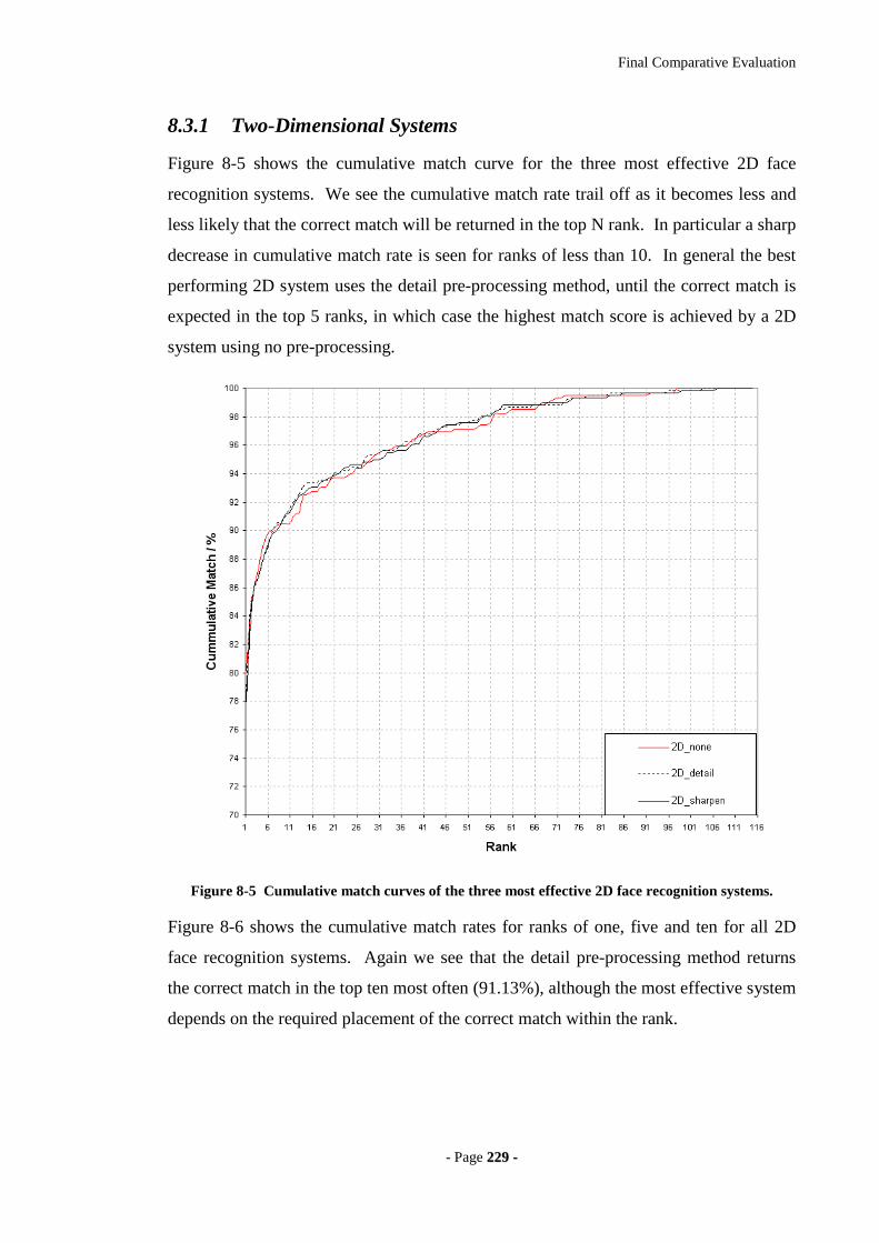
Final Comparative Evaluation
- Page 222299 --
8.3.1 Two-Dimensional Systems
Figure 8-5 shows the cumulative match curve for the three most effective 2D face
recognition systems. We see the cumulative match rate trail off as it becomes less and
less likely that the correct match will be returned in the top N rank. In particular a sharp
decrease in cumulative match rate is seen for ranks of less than 10. In general the best
performing 2D system uses the detail pre-processing method, until the correct match is
expected in the top 5 ranks, in which case the highest match score is achieved by a 2D
system using no pre-processing.
Figure 8-5 Cumulative match curves of the three most effective 2D face recognition systems.
Figure 8-6 shows the cumulative match rates for ranks of one, five and ten for all 2D
face recognition systems. Again we see that the detail pre-processing method returns
the correct match in the top ten most often (91.13%), although the most effective system
depends on the required placement of the correct match within the rank.
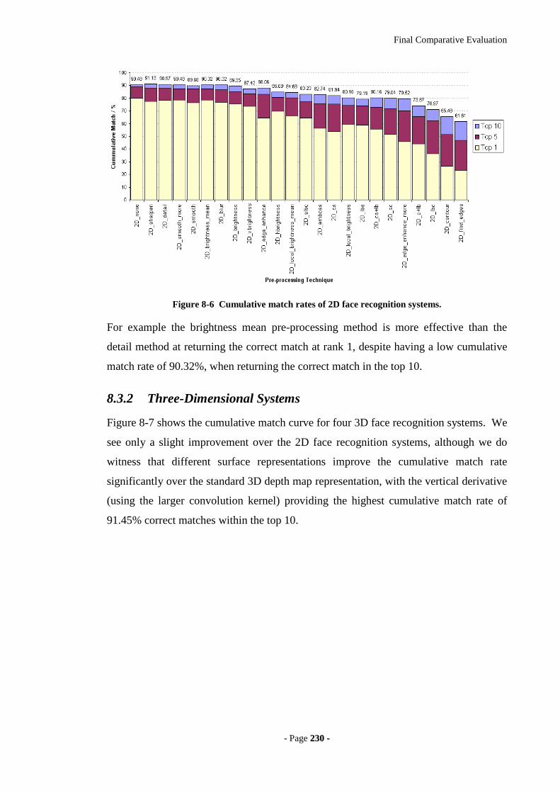
Final Comparative Evaluation
- Page 223300 --
Figure 8-6 Cumulative match rates of 2D face recognition systems.
For example the brightness mean pre-processing method is more effective than the
detail method at returning the correct match at rank 1, despite having a low cumulative
match rate of 90.32%, when returning the correct match in the top 10.
8.3.2 Three-Dimensional Systems
Figure 8-7 shows the cumulative match curve for four 3D face recognition systems. We
see only a slight improvement over the 2D face recognition systems, although we do
witness that different surface representations improve the cumulative match rate
significantly over the standard 3D depth map representation, with the vertical derivative
(using the larger convolution kernel) providing the highest cumulative match rate of
91.45% correct matches within the top 10.
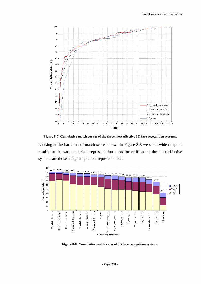
Final Comparative Evaluation
- Page 223311 --
Figure 8-7 Cumulative match curves of the three most effective 3D face recognition systems.
Looking at the bar chart of match scores shown in Figure 8-8 we see a wide range of
results for the various surface representations. As for verification, the most effective
systems are those using the gradient representations.
Figure 8-8 Cumulative match rates of 3D face recognition systems.
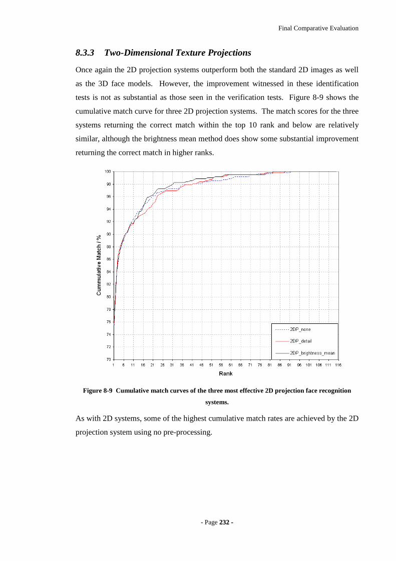
Final Comparative Evaluation
- Page 223322 --
8.3.3 Two-Dimensional Texture Projections
Once again the 2D projection systems outperform both the standard 2D images as well
as the 3D face models. However, the improvement witnessed in these identification
tests is not as substantial as those seen in the verification tests. Figure 8-9 shows the
cumulative match curve for three 2D projection systems. The match scores for the three
systems returning the correct match within the top 10 rank and below are relatively
similar, although the brightness mean method does show some substantial improvement
returning the correct match in higher ranks.
Figure 8-9 Cumulative match curves of the three most effective 2D projection face recognition
systems.
As with 2D systems, some of the highest cumulative match rates are achieved by the 2D
projection system using no pre-processing.
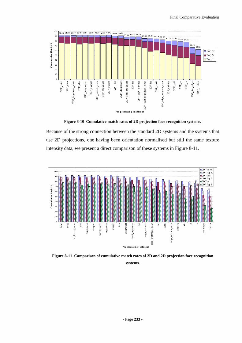
Final Comparative Evaluation
- Page 223333 --
Figure 8-10 Cumulative match rates of 2D projection face recognition systems.
Because of the strong connection between the standard 2D systems and the systems that
use 2D projections, one having been orientation normalised but still the same texture
intensity data, we present a direct comparison of these systems in Figure 8-11.
Figure 8-11 Comparison of cumulative match rates of 2D and 2D projection face recognition
systems.
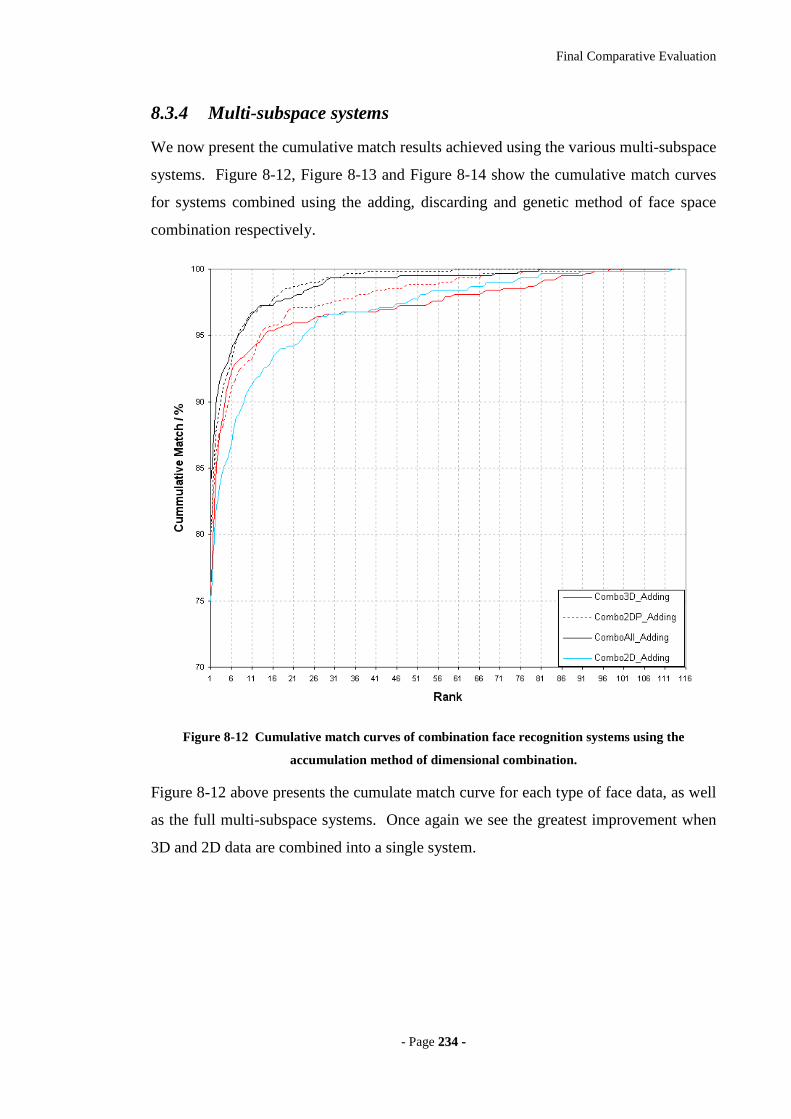
Final Comparative Evaluation
- Page 223344 --
8.3.4 Multi-subspace systems
We now present the cumulative match results achieved using the various multi-subspace
systems. Figure 8-12, Figure 8-13 and Figure 8-14 show the cumulative match curves
for systems combined using the adding, discarding and genetic method of face space
combination respectively.
Figure 8-12 Cumulative match curves of combination face recognition systems using the
accumulation method of dimensional combination.
Figure 8-12 above presents the cumulate match curve for each type of face data, as well
as the full multi-subspace systems. Once again we see the greatest improvement when
3D and 2D data are combined into a single system.
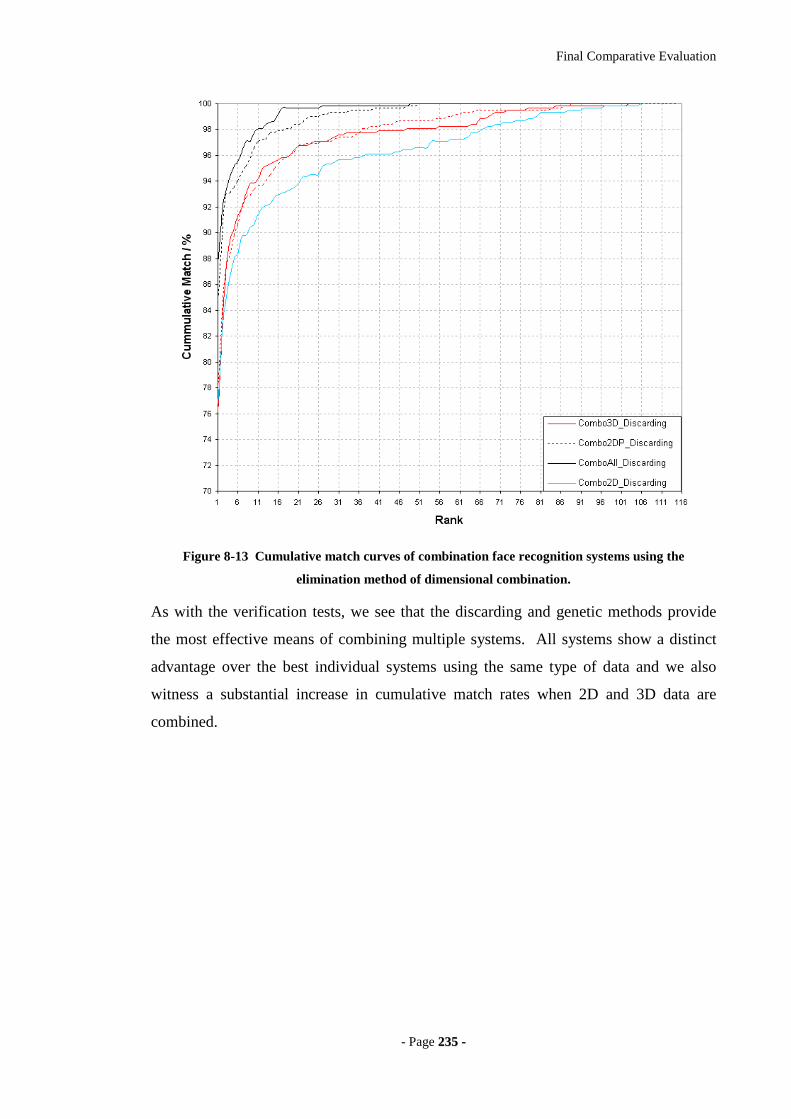
Final Comparative Evaluation
- Page 223355 --
Figure 8-13 Cumulative match curves of combination face recognition systems using the
elimination method of dimensional combination.
As with the verification tests, we see that the discarding and genetic methods provide
the most effective means of combining multiple systems. All systems show a distinct
advantage over the best individual systems using the same type of data and we also
witness a substantial increase in cumulative match rates when 2D and 3D data are
combined.
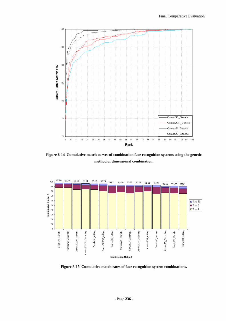
Final Comparative Evaluation
- Page 223366 --
Figure 8-14 Cumulative match curves of combination face recognition systems using the genetic
method of dimensional combination.
Figure 8-15 Cumulative match rates of face recognition system combinations.
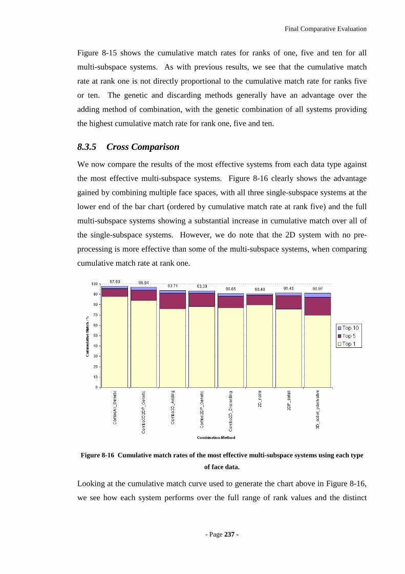
Final Comparative Evaluation
- Page 223377 --
Figure 8-15 shows the cumulative match rates for ranks of one, five and ten for all
multi-subspace systems. As with previous results, we see that the cumulative match
rate at rank one is not directly proportional to the cumulative match rate for ranks five
or ten. The genetic and discarding methods generally have an advantage over the
adding method of combination, with the genetic combination of all systems providing
the highest cumulative match rate for rank one, five and ten.
8.3.5 Cross Comparison
We now compare the results of the most effective systems from each data type against
the most effective multi-subspace systems. Figure 8-16 clearly shows the advantage
gained by combining multiple face spaces, with all three single-subspace systems at the
lower end of the bar chart (ordered by cumulative match rate at rank five) and the full
multi-subspace systems showing a substantial increase in cumulative match over all of
the single-subspace systems. However, we do note that the 2D system with no pre-
processing is more effective than some of the multi-subspace systems, when comparing
cumulative match rate at rank one.
Figure 8-16 Cumulative match rates of the most effective multi-subspace systems using each type
of face data.
Looking at the cumulative match curve used to generate the chart above in Figure 8-16,
we see how each system performs over the full range of rank values and the distinct
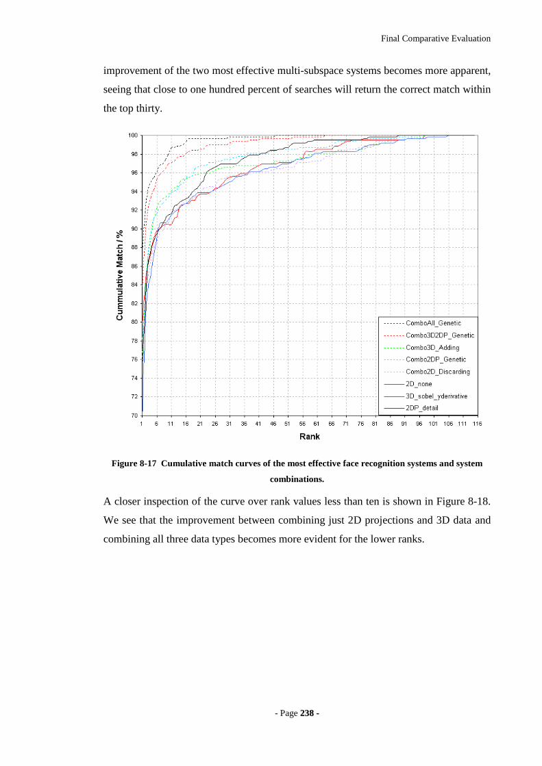
Final Comparative Evaluation
- Page 223388 --
improvement of the two most effective multi-subspace systems becomes more apparent,
seeing that close to one hundred percent of searches will return the correct match within
the top thirty.
Figure 8-17 Cumulative match curves of the most effective face recognition systems and system
combinations.
A closer inspection of the curve over rank values less than ten is shown in Figure 8-18.
We see that the improvement between combining just 2D projections and 3D data and
combining all three data types becomes more evident for the lower ranks.
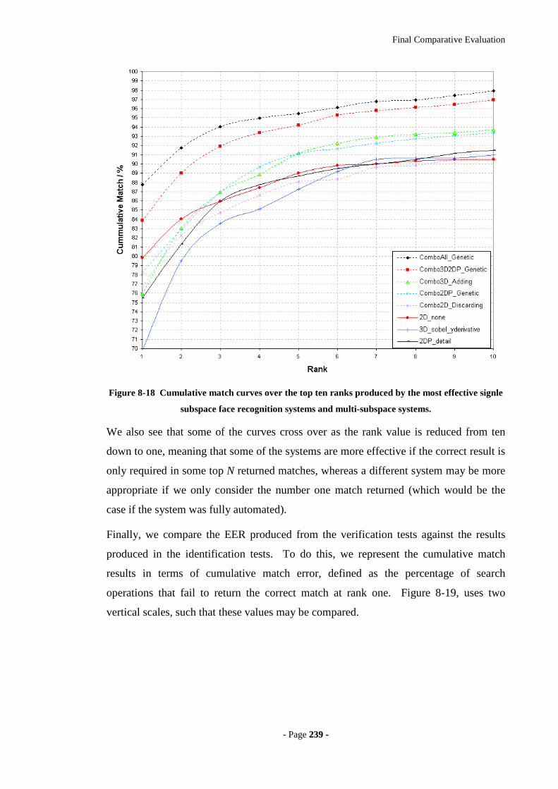
Final Comparative Evaluation
- Page 223399 --
Figure 8-18 Cumulative match curves over the top ten ranks produced by the most effective signle
subspace face recognition systems and multi-subspace systems.
We also see that some of the curves cross over as the rank value is reduced from ten
down to one, meaning that some of the systems are more effective if the correct result is
only required in some top N returned matches, whereas a different system may be more
appropriate if we only consider the number one match returned (which would be the
case if the system was fully automated).
Finally, we compare the EER produced from the verification tests against the results
produced in the identification tests. To do this, we represent the cumulative match
results in terms of cumulative match error, defined as the percentage of search
operations that fail to return the correct match at rank one. Figure 8-19, uses two
vertical scales, such that these values may be compared.
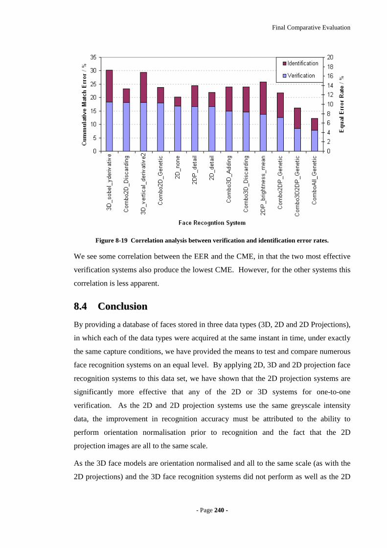
Final Comparative Evaluation
- Page 224400 --
Figure 8-19 Correlation analysis between verification and identification error rates.
We see some correlation between the EER and the CME, in that the two most effective
verification systems also produce the lowest CME. However, for the other systems this
correlation is less apparent.
88..44 CCoonncclluussiioonn
By providing a database of faces stored in three data types (3D, 2D and 2D Projections),
in which each of the data types were acquired at the same instant in time, under exactly
the same capture conditions, we have provided the means to test and compare numerous
face recognition systems on an equal level. By applying 2D, 3D and 2D projection face
recognition systems to this data set, we have shown that the 2D projection systems are
significantly more effective that any of the 2D or 3D systems for one-to-one
verification. As the 2D and 2D projection systems use the same greyscale intensity
data, the improvement in recognition accuracy must be attributed to the ability to
perform orientation normalisation prior to recognition and the fact that the 2D
projection images are all to the same scale.
As the 3D face models are orientation normalised and all to the same scale (as with the
2D projections) and the 3D face recognition systems did not perform as well as the 2D
Final Comparative Evaluation
- Page 224411 --
or 2D projections, this demonstrates that 3D face shape alone is not as discriminating as
colour and texture information.
However, this is providing the lighting conditions are relatively controlled. As each set
of faces for each person in the database were captured in the same session without
altering the lighting conditions, this did give the 2D face recognition systems a slight
advantage, as one of the key reasons for using surface shape alone in 3D face
recognition systems is to create a face recognition system that is invariant to variations
in lighting conditions. This is perhaps the reason behind the anomaly witnessed in the
identification experiments, where the 2D system with no pre-processing emerged as the
most effective for rank-one identification (except for combinations of 2D and 3D
systems). It is possible that this 2D system is using the lighting conditions on the face
as a cue for recognition and that because these lighting conditions may be quite unique
(due to the slow progressive changes in lighting throughout the captures sessions and
the height of the person meaning overhead lighting is reflected differently) they are very
useful for selecting a rank-one match. Whereas in order to achieve the higher
cumulative match rates for larger rank values, the system must be less reliant on the
chance that the lighting has remained constant and therefore other systems take the lead,
as seen when considering matches in the top ten: the 2D none system becomes the least
effective.
We have shown that combining multiple systems provides substantial benefits in terms
of verification and identification capabilities. In almost all cases combining multiple
systems provides a reduction in EER and CME, when compared to all individual
systems using the same type of data. A much greater improvement is then provided
when we bridge the gap between 2D and 3D data, by combining systems across these
data types. Combining 2D projection systems with 3D systems reduced the EER to
4.84% and improves the CMR-10 to 96.94%. The further improvement introduced
when standard 2D systems are included in the combination could be due to an increased
robustness to small inaccuracies in orientation normalisation (2D images are aligned by
the eyes rather than the nose tip), by effectively providing an alternative method of
alignment. Secondly, the orientations at which different people naturally position their
head may also be used as a cue for recognition. It may also be that variations in lighting
from one data collection location to another (represented in 2D images by small areas of

Final Comparative Evaluation
- Page 224422 --
background in the corners of the image) could aid recognition, as no subject was present
in more than one capture location.

Final Conclusions and Future Work
- Page 224433 --
99 FFiinnaall CCoonncclluussiioonnss aanndd FFuuttuurree WWoorr kk
We now bring a close to this thesis by summarising the discoveries and achievements
made throughout our research. In chapter 1 we outlined a number of goals that we
hoped to achieve and we now begin this chapter by considering our progress towards
each of these goals in relation to the relevant sections of this thesis. We then discuss
each of the technologies explored, again referring to individual chapters, summarising
the progress made. Finally, we draw overall conclusions from the results obtained and
predict their impact on the research field, before suggesting the most promising avenues
of future research.
99..11 PPrr ooggrr eessss AAcchhiieevveedd
Give an overview of existing face recognition systems and the current state of
research in this field.
In section 3 we reviewed the current literature regarding face recognition technology
and identified a number of promising methods worthy of further investigation. In
particular we focused on PCA and LDA approaches, such as the Eigenface and
Fisherface methods as discussed in sections 4.3 and 4.4 respectively. We carried out
experiments similar to those of other researches, reconfirming results on a standard
dataset and began to explore some ways of improving these systems.
Identify the problems associated with existing face recognition systems and
possible avenues of research that may help to address these issues.
Among the available literature it was clear that several issues had become well known
as primary hindrances to face recognition systems, namely variations in lighting
conditions, facial expressions and head orientation. Although there are several other
problems that will eventually need to be addressed, such as facial occlusion, disguises
(beards, glasses, headwear) and aging, these are generally considered secondary
(perhaps because they are more difficult). Obviously, it is accepted that a face cannot
be recognised if it cannot be seen, but an ideal surveillance application should be able to
cope with these secondary problems. However, a great deal of improvement was
Final Conclusions and Future Work
- Page 224444 --
needed in terms of coping with lighting, facial expression and head orientation before
these more difficult problems could be addressed.
Improve the effectiveness of existing face recognition algorithms, by introduction
of additional processing steps or adaptation of the method.
In order to improve a systems ability to cope with variations in lighting we explored the
area of image pre-processing in section 4.5, in an attempt to normalise lighting
conditions while maximising between-class variation. We identified a number of pre-
processing methods that reduced error rates for the eigenface system, presented in
section 4.6. We then addressed the problem of expression by further developing the
statistical analysis used in producing the model for discrimination. Approaches such as
the Fisherface method allowed for multiple representations of the same face in order to
capture such within-class variation, which we explored in detail in section 4.4, again
showing how image pre-processing can reduce error rates.
Design and implement novel face recognition approaches, taking advantage of the
newly emerging 3D-capture technology.
In order to address the problem of head orientation, we began an investigation into the
use of 3D capture technology to aid face recognition in section 5. Using 3D face
models we were able to normalise facial orientation using the techniques described in
section 5.2, to perform recognition on face depth maps as explained in section 5.3.1.
We continued this research direction using the experience gained in 2D face recognition
investigations; we applied various pre-processing methods to produce numerous 3D
surface representations, again producing a reduction in error rates. The resultant system
was able to perform face recognition to a high level of accuracy, with much improved
robustness to head orientation, as presented in section 5.3.
The 3D face database also allowed for projection of the 2D texture from an orientation
normalised 3D model. This facilitated creation of a third novel type of face recognition
system, using 2D techniques applied to an orientation normalised 2D image, created
using some of the advantages offered in 3D systems, as shown in section 6.1. In an
attempt to utilise multiple approaches to improve error rates, we developed new
methods of combining systems (section 7), taking advantages of 3D and 2D data and a
range of pre-processing methods in a single system.
Final Conclusions and Future Work
- Page 224455 --
Finally, returning to the first principles of 3D face recognition to develop a new
recognition algorithm aside from the subspace PCA and LDA approaches used in
previous chapters, we developed the novel IRAD contours methods of face recognition
(see section 5.7).
Analyse and evaluate a range of face recognition systems applied to both two-
dimensional and three-dimensional data.
Because 3D face recognition was relatively unexplored we collected a large database of
3D face models to train and test 3D face recognition systems. This database will
provide a great resource for research into the areas of 3D and 2D face recognition. As
the database includes 2D images, captured alongside the 3D face models it allows a
direct comparison of the two types of face data. We carried out investigations using the
same PCA and LDA approaches applied to 3D face data and the corresponding 2D face
data and presented the results in section 8.
Determine the most effective method of combining the range of face recognition
techniques, in order to achieve a more effective face recognition system.
It became clear in section 7.2 that although combining multiple face recognition
systems could reduce error rates, the degree of this improvement was dependent on the
method of criteria used for combination. In section 7.3 we developed and tested three
methods of combination. The results presented demonstrated that the most effective
method of the three was to use a genetic algorithm to optimise the combination.
However, in section 7.5 we were able to demonstrate that even this improvement could
be surpassed by some human intuition and that a more effective genetic algorithm
would likely be discovered with some additional investigation.
Evaluate this final face recognition system and present results in a standard
format.
In chapter 8 we defined standard training and test sets from the 3D face database, in
which each image was represented by a 3D face model, 2D image and 2D texture
projection. We then selected numerous face recognition systems and compared the
performance on this triple modal database. The results are presented in such formats as
to be easily compared to the majority of face recognition publications.
Final Conclusions and Future Work
- Page 224466 --
Identify limitations of the final face recognition system and propose a line of
further research to combat these limitations.
In section 9 we describe some of the difficulties still faced by face recognition systems.
We suggest points at which our own research may be extended to explore these
problems and what other technologies are required in order to increase the capabilities
of face recognition systems.
99..22 22DD FFaaccee RReeccooggnnii tt iioonn
We began by exploring the eigenface method of face recognition, implementing a
standard system using no image pre-processing to produce an EER of 34.0%. Further
investigation showed that some pre-processing techniques could greatly reduce error
rates and without any alterations to the eigenface technique itself, an EER of 22.4%
percent can be achieved (a reduction of 11.6%). We published these findings in the
conference proceedings of the International Conference on Image and Graphics.
Although the test set used in these experiments contained a majority of extremely
difficult images (20% of the images are partially obscured and 40% of the images have
extreme lighting conditions), an error rate in which one in five verifications produces an
incorrect decision is not suitable for most potential face recognition applications.
However, this investigation did prove that selecting a suitable image pre-processing
technique is vital to the performance of a face recognition system.
Continuing research focused on appearance based approaches leading towards the
Fisherface method, which is widely reported to produce superior recognition accuracy
than the eigenface method when multiple examples of the same subject are available for
training. However, our initial experiments did not comply with these findings. Further
investigation showed that by altering the training and test sets such that they both
represented the same capture conditions produced significantly better results.
Therefore, if the Fisherface method is to be used in a real world scenario, it is vital that
the training set is an adequate representation of the expected application data. Providing
such a training set is available, the Fisherface method has significantly lower error rates
(20.1%) than both the eigenface (25.5%) and direct correlation methods (25.1%) applied
to the same test set. Hypothesising that the Fisherface method would be as dependent
on the image pre-processing techniques as the eigenface method, we tested the same
Final Conclusions and Future Work
- Page 224477 --
processing techniques as in previous experiments, reducing the EER to 17.8%. We
compared the Fisherface and eigenface methods in detail in section 4.6 (also published
in ‘Face Recognition: A Comparison of Appearance-Based Approached’ [ 15 ] and
presented at the International Conference on Digital Image Computing: Techniques and
Applications. These investigations supported the consensus that Fisherface systems
typically produce lower error rates than eigenface. Although an additional key finding
was that lighting correction techniques (colour normalisation etc.) have less affect than
application of LDA to model such variations.
99..33 33DD FFaaccee RReeccooggnnii tt iioonn
Because of the success of PCA and LDA appearance-based approaches to two-
dimensional face recognition, we adapted these methods for application to 3D face data.
This required implementation of an orientation normalisation routine, to localise the
nose of the 3D face model and orientate the facial surface to a fronto-parallel
orientation, before producing a depth map of the 3D face model. Applying PCA to
these depth maps we introduced the eigensurface method of face recognition, which was
capable of recognising faces with substantially lower error rates (12.7% EER) than the
best two-dimensional systems (20.4% EER and 17.8% EER). These promising results
(published in [ 16 ]) demonstrated that geometric face structure is useful for recognition
when used independently from colour and texture and capable of achieving high levels
of accuracy, suggesting that 3D face recognition has distinct advantages over
conventional two-dimensional approaches.
To follow on the success of applying PCA to facial surface representations we
continued along the same course of research as applied to two-dimensional systems by
examining the application of LDA to 3D surface representations. The EER produced
using the best surface representations was 11.3% EER, again demonstrating the superior
performance of LDA when compared with PCA approaches, as well as reinforcing
earlier findings that 3D face recognition could produce better results than corresponding
two-dimensional Fisherface systems (17.8% EER). The experiments carried out to
produce these results are documented in detail in section 5 (also published in [ 17 ]).
Given that the 3D capture method produces face models invariant to lighting conditions
Final Conclusions and Future Work
- Page 224488 --
and provides the ability to recognise faces regardless of pose, this system is particularly
suited for use in security and surveillance applications.
Rather than focus purely on subspace-based approaches to 3D face recognition we also
developed a novel method capable of recognising faces based on cues extracted from
both the colour and geometric shape data available in 3D face models. One of the key
advantages of our IRAD contours method is that it uses relatively little registration in
terms of feature detection and image alignment. Once this single feature localisation
operation has been performed all variances due to head orientation are reduced to a one-
dimensional shift in a simple cross-correlation process. Using this technique we were
able to show that a single contour around the tip of the nose contained enough
discriminatory information to perform recognition with an EER of just 21.91%.
Although we were restricted by time limitations to explore this method in great detail,
we were able to apply a simple weighted sum across signal ensemble correlation scores,
reducing the EER to 20.02%, although much greater reductions are expected if colour
and texture information were included and additional constraints applied.
Finally, we investigated a method that perhaps lies at a midpoint between two-
dimensional and 3D face recognition. By using a texture mapped 3D face model we
produced system that was able to orientate the face to a fronto-parallel orientation
before projecting the texture back into the 2D image plane. This 2D image could then
be used for recognition as with standard two-dimensional face recognition methods.
We have demonstrated that such 2D projection systems have significant advantages
over standard 2D systems: in almost all cases the error rates are significantly lower than
the equivalent system without 3D orientation. This emphasises the importance of
orientation normalisation for recognition and that the use of absolute size (2D
projections are real-size) as a feature for recognition can provide additional
discriminatory information.
However, an additional side-effect of 2D projection systems, which may also have
improved results, is that surface noise in terms of depth precision errors are effectively
compressed onto a 2D plane. Because no virtual lighting or surface shading effects are
used, any error in surface depth is not visible in the 2D image projection. Perhaps with
a better method of dealing with surface noise in 3D methods we would see substantial
improvements.
Final Conclusions and Future Work
- Page 224499 --
99..44 MM uull tt iippllee SSuubbssppaaccee CCoommbbiinnaatt iioonnss
By applying FLD as an analysis tool to individual face space dimensions we were able
to confirm that although an image subspace may not perform well when used for
recognition, it may still contain discriminatory components that could complement other
face space systems. Hence we uncovered the potential to improve recognition error
rates by combining multiple dimensions from a range of face recognition systems.
Combining multiple systems in this way has been shown to be highly beneficial when
used with the best single-subspace eigenface system, reducing the EER from 19.7% to
15.4%. Although when the same method was applied to the Fisherface systems, little
influence was witnessed. These initially confusing results lead to further investigation
into the methods of combination and weighting schemes applied. By using the EER as
combination criteria, we were able to demonstrate that a Fisherface system could also be
improved in the same way, reducing the EER from 17.8% using the best processing
technique down to 12.8% for the multi-subspace. We submitted the findings from this
investigation to BMVC 2004, which were later published in the conference proceedings
[ 21 ].
Naturally, this method of system combination could also be extended to the appearance-
based 3D systems, which we tested using a variety of distance metrics, to discover that
the cosine distance metric was the most suitable for dimensional combination. Out of
the seventeen surface spaces (with forty-nine dimensions in each one) sixteen subspaces
were shown to provide at least one useful dimension, totalling 184 dimensions in the
final composite surface space. This combination process was able to reduce the EER
from 11.5% to 9.3% EER, which is explained in more detail in section 7.2.
The final application of combining multiple subspaces was to combine 3D and 2D
systems in order to create a face recognition method that utilises both 3D geometric
shape and 2D texture information together with the ability to perform orientation
normalisation. This combination managed to reduce the EER to 4.84%. These error
rates are state-of-the-art, particularly when considering that this is applied to test sets
with variations in head orientation and the increased robustness to lighting variation due
to the use of geometric shape data. However, it is likely that further reductions are still
possible using a similar method of dimensional combination. This prediction is
extrapolated from the realisation that the combination of two-dimensional systems is not
Final Conclusions and Future Work
- Page 225500 --
optimal. Even though the combination contains various dimensions from all twenty-
four 2D systems (producing 10.33% EER), a simple intuitive selection of all dimensions
from just four systems produces a lower EER of 9.26%. This suggests that an improved
combination process could be derived from the principles used in the intuitive selection
(four of the best systems using very different pre-processing techniques). Because this
improved combination, utilising only four face spaces performs so well, it raises the
question as to whether these four image types could be combined prior to LDA. This
would not be possible using all pre-processing techniques as the high time space
complexity makes the process intractable, but it may produce a more efficient subspace
for recognition than combining the dimensions after training.
Surprisingly, this is not the case. We see that pre-training combination produces a
higher EER of 9.66% than those produced by combining the four systems after training.
We hypothesise that the reason for the improved results of the post-training
combination is due to the use of two disjoint training sets: one to compute the projection
matrices and the second as a double check before combining only the most
discriminatory dimensions. Perhaps by concatenating four images before applying
LDA we supplied so much information that the system effectively over-trains on the
single training set, but forcing four separate systems to rely on less information and then
combining on a separate secondary training set reduces any over-training that may have
occurred in the preliminary LDA.
99..55 CCoommppaarr aatt iivvee EEvvaalluuaatt iioonn
The penultimate chapter of our thesis provided a final evaluation across three data types
(3D, 2D and 2D Projections), in which each of the data types were acquired at the same
instant in time, providing the means to test and compare numerous face recognition
systems on an equal level. This was done to recompense the inability to directly
compare some of the results from the various experiments throughout our research. We
included an additional measure of system effectiveness in the form of a cumulative
match curve, in order to demonstrate a systems ability to perform at the task of
identification when searching through a database of known faces.
The ability to directly compare the results from numerous systems has allowed for some
interesting conclusions. We see that the 2D projection systems are significantly more
Final Conclusions and Future Work
- Page 225511 --
effective than any of the 2D or 3D systems for one-to-one verification. Because these
two types of system are actually using the same greyscale intensity data, the
improvement in recognition accuracy can only be attributed to the orientation
normalisation procedure and the consistent scale of 2D projections. Conversely,
because the 3D systems are also privy to these same advantages, but do not perform as
well as the 2D projections this demonstrates that 3D face shape alone is not as
discriminating as colour and texture information (providing the lighting conditions
remain constant).
The final evaluation also reconfirmed that combining multiple systems provides
substantial benefits for both verification and identification operations. The multi-
subspace using 2D, 3D and 2D projection data achieved a CMR of 96.94% correct
matches returned in the top ten.
99..66 FFuuttuurr ee RReesseeaarr cchh
The most effective face recognition system produced from our research has been the
multiple subspace combinations that combine Fisherface and Fishersurface systems
using 3D face models, 2D images and 2D texture projections into a single composite
subspace. Although we explored three methods of combination and identified the
genetic algorithm method as marginally the most effective, there is still a great deal of
development that may be done in this area. One brief experiment has already
demonstrated that an intuitive selection of just four subspaces can produce lower error
rates than the best combination produced by the GA, when applied to two-dimensional
systems. This suggests that altering the evolution functions used in the GA may
produce more effective combinations.
We would suggest that a coarse to fine evolution cycle might be more effective. Such a
system would begin by combining entire subspaces, rather than individual dimensions;
a single mutation would accumulate or discard all dimensions from an entire subspace
and crossover would select random subspaces as a whole from each parent. As the
fitness of the population reaches a plateau the mutation and crossover functions would
begin operating on a finer level, selecting smaller and smaller fractions of the subspaces
until individual dimensions were being selected or discarded.
Final Conclusions and Future Work
- Page 225522 --
Another area in which this combination approach may be expanded would be to create
subspace systems using partial sections of the original face image (or 3D surface).
Pentland et al [ 40 ] found that this approach was beneficial in their paper on modular
eigenface approaches, although they were not using the same criteria based dimensional
combination approach as described here. We have witnessed the same phenomena
(although from a different perspective) when we discovered that concatenating four
images before applying LDA, produced higher error rates than performing LDA on each
individual image and then combining the dimensions after the training phase. The same
may apply to an image of a single face: perhaps splitting the image into two parts and
then combining the resultant subspaces of each after LDA will produce a more effective
system. This approach could be performed on a large scale using the GA combination
algorithm. For example, supposing we applied all the same image pre-processing
techniques and 3D surface representations to images of the nose area alone (having
cropped out the cheeks, forehead and chin) producing a variety of nose-recognition
systems. These subspaces could then be included in the combination genome, doubling
the number of subspaces available and providing much larger scope for improvement.
We believe that such an approach could prove to be highly effective for the following
reasons:
• Different image pre-processing techniques and surface representations
are likely to be particularly well suited to specific areas of the face (edge
detectors around the eyes, colour normalisation for the cheeks, gradient
representations for the nose for example).
• By reducing the size of the image to focus on a smaller area of the face
but maintaining the size of the training set, we improve the ratio between
true discriminatory information and noise.
• By using multiple subspaces concentrated on partial regions of the face
we increase robustness against partial occlusion of one area, such as
glasses, hats or beards.
Another exciting area that we have not explored in this thesis is the possibility of using
multiple face recognition systems in series. This is a different approach to combining
multiple systems to make a single definitive decision, but rather to make an initial
Final Conclusions and Future Work
- Page 225533 --
screening step, before making the final accept/reject decision. Such an approach would
allow each face recognition system to concentrate on one aspect of the decision
problem. For instance, the primary face recognition system may be used to remove any
certain rejections, before the secondary system makes the final acceptance decision.
The threshold of the primary system would be configured such that the false rejection
rate was near zero and then used to prune the training set for the secondary system,
leaving only comparisons that looked similar. Using this two stage technique the
resultant secondary system would be specifically designed to determine the likeness of
two similar faces, knowing that it would never have to compare any drastically different
faces the subspace could be a more effective representation of the between class
differences.
One of the most interesting findings of our research was that the 2D projection systems
were the most effective means of recognising faces. However, the test set on which
these results were based did not contain any controlled variations in lighting conditions.
Therefore, lighting typically remained constant for each person and might also have
contributed as cues for recognition. One of the key advantages of using 3D face models
is that basing the recognition on shape rather than colour and texture means that the
system becomes invariant to lighting conditions (providing the 3D camera is still
capable of constructing a 3D model), but this advantage is lost when reverting back to
texture data of 2D projections. One method of combating this problem would be to use
the 3D model shape to facilitate lighting correction. As any two-dimensional image
pre-processing technique can only adjust colour and intensity levels without taking into
account the shadow and shading due to the surface shape of the face, it becomes very
difficult to reproduce or compensate for specific lighting conditions. However, by
using the 3D face model to generate virtual lighting on the textured surface it becomes
possible to normalise lighting across the 3D surface or simulate the same lighting
conditions from one face onto another.
The IRAD contours method as described in section 5.7 has only been touched upon in
this thesis. Unfortunately, the technique was only conceived towards the end of our
research project and we now leave the full potential of this method to be exposed by
another researcher. There are two immediate topics that must be addressed. Firstly, to
test the effect of constraining correlation of multiple contour signals to have the same

Final Conclusions and Future Work
- Page 225544 --
rotational phase. The process described in section 5.7.5 allowed each individual signal
to correlate independently, meaning that the highest correlations of two signals may
compete with different phase shifts, hence allowing greater flexibility for incorrect
matches to achieve a higher correlation score. Secondly, no colour or texture
information was extracted for use in the signal correlation stage. Since this information
has been shown to be of great benefit when combining 2D and 3D subspaces it is highly
likely that similar improvements will be seen for this method.
Further improvements to the IRAD contours method would be expected by performing
some statistical analysis on the discriminatory nature of the various facial contours and
the relative dependence on such features as curvature, symmetry, texture and facial
location. We have already witnessed that weighting contours signals according to the
distance from the contour origin has a beneficial effect, but there are likely to be other
such dependencies. The systems ability to cope with changes in expression must also
be investigated. Whereas with LDA approaches we are able to represent and model
within-class variation (including expression to some extent), this is currently not
featured in the IRAD contours method. There are numerous possibilities that may
contain some potential to overcome these difficulties, such as correlating on partial
signals extracted from rigid facial areas whilst ignoring those from malleable regions, or
modelling signal variation due to expression by LDA or some other statistical method.

Appendices
- Page 225555 --
1100 AAppppeennddiicceess
I - 3D FACE DATABASE STORAGE
Master copies of the database will be held by Cybula Ltd. and made available by secure
download (access via username and password) and/or DVD library, agreed with Cybula
beforehand. No information revealing the subject identity will be stored with the data.
Agreement signatures will be held separately by Cybula Ltd. and not distributed to any
other party. No data may be redistributed by anybody other than Cybula Ltd.
Each 3D face model will be stored under a filename using the naming convention
shown in Appendix II. For example, a file stored under the name ‘00021-10-
mww24bnncy.obj’ is a Wavefront OBJ file containing a 3D model of a 24 year old (24)
white (ww) male (m), who does have a beard, but is not wearing glasses or headwear
(bnn) and facing forwards with a neutral expression (-10-). Colour texture is available
(c) for the model (stored under filename 00021-10-mww24bnncy.bmp) and permission
has been given for his image to be published (y). All other files in the database
containing “00021-“ contain models of the same person. A text file will be stored with
the model under filename 00021-10-mww25bnncy.txt, containing the following
information.
Subject ID 00021
Model ID 10
Capture Conditions Front facing, neutral expression .
Sex m
Ethnicity White
Age 24 years
Subject was wearing:
No Beard
No hat
No glasses
Height: 5'10"
Weight: 75 Kg
More....
Subject has given permission to publish his/her ima ge in
scientific papers and journals
Colour texture is not available

Appendices
- Page 225566 --
II - 3D FACE DB METADATA
Filename nnnnn-xx-srraaeeetp.ext
nnnnn Five digit unique subject identifier.
Xx Two digit capture condition identifier as specified in Table 5-1.
S Single character indicating gender. m = male, f = female
Rr
Two character label indicating ethnicity:
ww White
ap Asian Pakistani
ab Asian Bangladeshi
ai Asian Indian
ac Asian Chinese
aj Asian Japanese
ao Asian Other
na American Indian
ng Aboriginal
bb Black British
bc Black Caribbean
ba Black African
bo Black Other
hs Hispanic Spanish
hm Hispanic Mexican
hp Hispanic Puerto Rican
hc Hispanic Cuban
ho Hispanic Other
mm Mixed
oo Other / Abstain
Aa Two digit number indicating age, calculated from the DOB entry.
eee
Three character label indicating presence of external features:
b = beard present, n = not present
g = glasses present, n = not present
h = headwear present, n = not present
t Single character indicating the type of texture available for that model:
g = greyscale texture, c = colour texture, n = no texture
p
Single character flag indicating whether permission for publication has been
granted.
y = publication permissions granted.
n = publication permissions not granted.
ext
Three character extension, indicating the file type.
obj = The 3D Face Mode file.
bmp = The 2D bitmap texture file.
sp1 = Intermediate 3D reconstruction file.
sp2 = Intermediate 3D reconstruction file.
txt = The questionnaire information file.
Table 10-1 File storage convention used for the UOY 3D Face Database.

Appendices
- Page 225577 --
III - AURA GRAPH MATCHER RESULTS
Proof-of-concept tests were carried out using a small database of facial surfaces,
comprising 4 models of one person (A1, A2, A3, A4) and four models of other people
(B1, C1, D1, E1) [ 46 ][ 47 ]. Graph nodes are selected from the vertices of the facial
surfaces (no feature detection is attempted). For training, the graphs are fully connected
and the edges labelled with the distances between nodes. The AURA graph matcher is
then trained to recognise the 8 facial surfaces.
Identification tests are carried out by performing identification operations using four
models of one subject from the database (A1, A2, A3, A4), at various levels of
quantisation.
Quantisation Query Matches (Strength)
0.001 A1 A1(100%), A2(100%) A2 A2(100%) A3 A3(100%) A4 Out of memory 0.01 A1 A1(100%), A2(100%), A3(100%), B1(100%) A2 A2(100%) A3 Out of memory A4 Out of memory 0.05 A1 A1(100%), A2(100%), A3(100%), A4(100%), B1(100%) A2 Out of memory A3 Out of memory A4 Out of memory
Table 10-2 – Results of proof-of-concept identification tests using the AURA graph matcher taken
from Turner [ 47 ].
We see in many cases that the algorithm halted due to insufficient memory before
completing the identification: this is due to instability in the current stage of AURA
development. Other results show that the query model matches perfectly with itself in
all cases, as would be expected. Three queries also return correct matches with other
face models of the same person, while two false matches are also witnessed.

Appendices
- Page 225588 --
IV – VERIFICATION ERROR RATES OF 2D MULTI-SUBSPACE SYSTEM
Multi-subspace 2D Date: Fri, 23 Jul 2004 06:50:23 Test Set B EER 10.4215 Minimum 0.0864 Maximum 1.4969 Threshold FRR FAR Threshold FRR FAR Threshold FRR FAR
0.0864 99.9604 0.0000 0.6882 14.7606 4.7280 1.0549 0.5144 78.4101 0.1006 99.8813 0.0000 0.6929 14.4044 5.0285 1.0690 0.3166 81.3830 0.1147 99.6438 0.0000 0.6976 14.0879 5.3372 1.0831 0.2374 84.0583 0.1288 99.4856 0.0000 0.7023 13.8504 5.6748 1.0972 0.0791 86.4844 0.1429 98.9315 0.0000 0.7070 13.6526 6.0071 1.1113 0.0000 88.6950 0.1570 98.0214 0.0000 0.7117 13.3755 6.3446 1.1254 0.0000 90.6443 0.1711 96.8738 0.0000 0.7164 13.0985 6.6994 1.1396 0.0000 92.2887 0.1852 95.2909 0.0000 0.7211 12.7820 7.1073 1.1537 0.0000 93.7388 0.1993 93.5892 0.0000 0.7258 12.3467 7.5223 1.1678 0.0000 94.9382 0.2134 90.8192 0.0000 0.7305 12.1884 7.9452 1.1819 0.0000 95.9797 0.2275 88.2074 0.0000 0.7352 11.7531 8.3872 1.1960 0.0000 96.8277 0.2416 86.0704 0.0000 0.7399 11.3573 8.8594 1.2101 0.0000 97.5144 0.2557 83.6565 0.0000 0.7446 10.8033 9.3366 1.2242 0.0000 98.0716 0.2698 80.8073 0.0000 0.7493 10.7638 9.8380 1.2383 0.0000 98.5241 0.2839 77.5623 0.0000 0.7540 10.4472 10.3642 1.2524 0.0000 98.8766 0.2980 74.5548 0.0007 0.7587 10.2097 10.8952 1.2665 0.0000 99.1621 0.3121 71.9430 0.0007 0.7634 9.9723 11.4386 1.2806 0.0000 99.3814 0.3262 67.8670 0.0015 0.7681 9.6953 12.0213 1.2947 0.0000 99.5330 0.3403 64.7012 0.0022 0.7728 9.3391 12.6552 1.3088 0.0000 99.6568 0.3544 60.7835 0.0041 0.7775 8.9830 13.2701 1.3229 0.0000 99.7519 0.3685 57.7760 0.0086 0.7822 8.5873 13.9197 1.3370 0.0000 99.8264 0.3826 54.6498 0.0120 0.7869 8.4685 14.5780 1.3511 0.0000 99.8814 0.3967 51.6423 0.0210 0.7917 8.2707 15.2774 1.3652 0.0000 99.9165 0.4108 48.9513 0.0318 0.7964 8.0332 15.9922 1.3793 0.0000 99.9446 0.4249 46.8935 0.0445 0.8011 7.8750 16.7433 1.3934 0.0000 99.9663 0.4390 44.5192 0.0610 0.8058 7.7562 17.5022 1.4075 0.0000 99.9794 0.4532 42.3427 0.0846 0.8105 7.4792 18.2978 1.4216 0.0000 99.9873 0.4673 40.0475 0.1141 0.8152 7.3209 19.0983 1.4357 0.0000 99.9940 0.4814 37.6336 0.1564 0.8199 6.8856 19.9481 1.4498 0.0000 99.9963 0.4955 35.8924 0.2002 0.8246 6.4899 20.8373 1.4639 0.0000 99.9981 0.5096 33.5180 0.2679 0.8293 6.2920 21.6920 1.4780 0.0000 99.9993 0.5237 31.6977 0.3604 0.8434 5.2632 24.5066 1.4922 0.0000 99.9996 0.5378 29.2046 0.4659 0.8575 4.8279 27.4574 0.5519 27.4238 0.5950 0.8716 4.3926 30.6671 0.5660 25.9596 0.7571 0.8857 4.2343 34.0482 0.5801 24.4954 0.9794 0.8998 3.9968 37.5712 0.5942 22.8334 1.2454 0.9139 3.4824 41.2311 0.6083 21.6462 1.5497 0.9280 3.1262 45.0089 0.6224 20.3403 1.9183 0.9421 2.8097 48.8496 0.6365 19.1927 2.3513 0.9562 2.4139 52.8179 0.6506 18.1243 2.8711 0.9703 1.8599 56.8064 0.6647 16.8579 3.5020 0.9844 1.5433 60.6741 0.6694 16.4622 3.7202 0.9985 1.3455 64.5398 0.6741 16.0269 3.9578 1.0126 1.0289 68.2997 0.6788 15.5916 4.2097 1.0267 0.7519 71.8746 0.6835 15.2750 4.4578 1.0408 0.5936 75.2640

Appendices
- Page 225599 --
V – VERIFICATION ERROR RATES OF 3D MULTI-SUBSPACE SYSTEM
Multi-subspace 3D Date: Sun, 11 Jul 2004 07:38:50 Test Set B EER 8.3869 Minimum 0.1000 Maximum 1.3873 Threshold FRR FAR Threshold FRR FAR Threshold FRR FAR
0.1000 99.9604 0.0000 0.6921 20.2216 1.8749 0.9410 2.5326 32.8675 0.1129 99.8417 0.0000 0.7050 18.1243 2.2083 0.9539 2.1765 36.7992 0.1257 99.8417 0.0000 0.7179 16.3435 2.5889 0.9667 2.0578 40.9770 0.1386 99.6834 0.0000 0.7222 15.9478 2.7266 0.9796 1.7808 45.2556 0.1515 99.5251 0.0000 0.7265 15.3542 2.8890 0.9925 1.4246 49.8073 0.1643 99.4460 0.0000 0.7307 15.0376 3.0496 1.0054 1.1080 54.4765 0.1772 99.0107 0.0000 0.7350 14.2857 3.2187 1.0182 0.8706 59.1611 0.1901 98.8128 0.0000 0.7393 13.8900 3.4114 1.0311 0.6727 63.7199 0.2030 98.4567 0.0000 0.7436 13.6526 3.5926 1.0440 0.4749 68.2649 0.2158 97.9818 0.0000 0.7479 13.3360 3.7816 1.0569 0.1583 72.6590 0.2287 97.2695 0.0000 0.7522 12.9402 3.9814 1.0697 0.1583 76.7018 0.2416 96.5968 0.0000 0.7565 12.5841 4.1928 1.0826 0.0791 80.3670 0.2545 95.7657 0.0000 0.7608 12.1092 4.4133 1.0955 0.0791 83.8080 0.2673 94.4994 0.0000 0.7651 11.9114 4.6498 1.1083 0.0791 86.8579 0.2802 92.9165 0.0000 0.7694 11.4365 4.8878 1.1212 0.0396 89.5419 0.2931 91.4127 0.0000 0.7737 11.1595 5.1336 1.1341 0.0000 91.7681 0.3059 90.1860 0.0007 0.7779 10.8429 5.4102 1.1470 0.0000 93.6692 0.3188 88.7218 0.0019 0.7822 10.6055 5.7182 1.1598 0.0000 95.2447 0.3317 86.7036 0.0022 0.7865 10.3680 6.0254 1.1727 0.0000 96.4598 0.3446 84.7250 0.0034 0.7908 9.9327 6.3607 1.1856 0.0000 97.4354 0.3574 82.8651 0.0045 0.7951 9.3787 6.7323 1.1985 0.0000 98.1921 0.3703 80.9260 0.0064 0.7994 8.9434 7.1069 1.2113 0.0000 98.7463 0.3832 78.8287 0.0097 0.8037 8.7455 7.4972 1.2242 0.0000 99.1557 0.3961 76.3356 0.0138 0.8080 8.5873 7.8936 1.2371 0.0000 99.4548 0.4089 73.7238 0.0183 0.8123 8.4685 8.2958 1.2499 0.0000 99.6456 0.4218 71.7056 0.0243 0.8166 8.0728 8.7371 1.2628 0.0000 99.7841 0.4347 69.0146 0.0307 0.8209 7.6771 9.1977 1.2757 0.0000 99.8642 0.4475 66.4424 0.0393 0.8251 7.4397 9.7011 1.2886 0.0000 99.9121 0.4604 63.7911 0.0543 0.8294 7.1626 10.1902 1.3014 0.0000 99.9517 0.4733 61.1397 0.0696 0.8337 6.9252 10.7294 1.3143 0.0000 99.9734 0.4862 58.3696 0.0898 0.8380 6.8065 11.3013 1.3272 0.0000 99.9869 0.4990 56.3910 0.1175 0.8423 6.6482 11.8832 1.3401 0.0000 99.9948 0.5119 52.9482 0.1486 0.8466 6.2525 12.4584 1.3529 0.0000 99.9970 0.5248 50.3759 0.1920 0.8509 5.9755 13.0938 1.3658 0.0000 99.9993 0.5377 47.5267 0.2305 0.8552 5.7776 13.7154 1.3787 0.0000 99.9996 0.5505 44.8753 0.2766 0.8595 5.3819 14.4070 0.5634 42.5406 0.3271 0.8638 5.0257 15.1180 0.5763 40.2849 0.3963 0.8681 4.8674 15.7920 0.5891 37.2774 0.4809 0.8723 4.6300 16.5662 0.6020 35.3383 0.5752 0.8766 4.5904 17.3622 0.6149 32.6474 0.6875 0.8809 4.4321 18.1743 0.6278 30.5501 0.8248 0.8852 4.2738 18.9998 0.6406 28.3340 0.9711 0.8895 4.1947 19.8856 0.6535 25.9992 1.1459 0.9024 3.6011 22.6998 0.6664 23.9019 1.3498 0.9153 3.2054 25.7733 0.6793 22.1607 1.5979 0.9281 2.7701 29.1788

Appendices
- Page 226600 --
VI – VERIFICATION ERROR RATES OF 2D PROJECTION MULTI-SUBSPAC E
SYSTEM
Multi-subspace 2DP Date: Wed, 14 Jul 2004 09:14:45 Test Set B EER 7.3385 Minimum 0.0699 Maximum 1.4772 Threshold FRR FAR Threshold FRR FAR Threshold FRR FAR
0.0699 99.9604 0.0000 0.6704 13.4943 2.7120 0.9988 0.4749 61.9468 0.0840 99.8813 0.0000 0.6751 12.9007 2.9115 1.0128 0.2770 65.8964 0.0981 99.6834 0.0000 0.6798 12.7028 3.1207 1.0269 0.2374 69.7124 0.1121 99.4460 0.0000 0.6845 12.3467 3.3355 1.0410 0.1979 73.3124 0.1262 98.7732 0.0000 0.6891 11.9905 3.5499 1.0550 0.0396 76.6962 0.1403 97.8631 0.0000 0.6938 11.5156 3.7797 1.0691 0.0396 79.8475 0.1544 96.9925 0.0000 0.6985 11.0803 4.0259 1.0832 0.0000 82.8361 0.1684 95.7657 0.0000 0.7032 10.6055 4.2935 1.0973 0.0000 85.4965 0.1825 94.3807 0.0000 0.7079 10.2097 4.5757 1.1113 0.0000 87.9207 0.1966 93.0748 0.0000 0.7126 9.7349 4.8986 1.1254 0.0000 90.0718 0.2106 91.2545 0.0000 0.7173 9.2996 5.2085 1.1395 0.0000 91.9676 0.2247 89.3945 0.0000 0.7220 9.1017 5.5303 1.1536 0.0000 93.5921 0.2388 87.3763 0.0000 0.7267 8.9038 5.8798 1.1676 0.0000 94.9569 0.2529 85.6351 0.0000 0.7314 8.4685 6.2425 1.1817 0.0000 96.0762 0.2669 83.2608 0.0000 0.7361 8.1124 6.6238 1.1958 0.0000 97.0335 0.2810 81.0447 0.0000 0.7407 7.6375 7.0197 1.2099 0.0000 97.7573 0.2951 78.2746 0.0000 0.7454 7.2418 7.4415 1.2239 0.0000 98.3336 0.3092 76.0190 0.0000 0.7501 6.7273 7.8906 1.2380 0.0000 98.7725 0.3232 73.3676 0.0007 0.7548 6.4108 8.3490 1.2521 0.0000 99.1228 0.3373 70.8746 0.0007 0.7595 6.1733 8.8366 1.2661 0.0000 99.3807 0.3514 67.9858 0.0015 0.7642 6.0546 9.3441 1.2802 0.0000 99.5622 0.3655 64.7804 0.0019 0.7689 5.7380 9.8444 1.2943 0.0000 99.7002 0.3795 61.8916 0.0037 0.7736 5.4610 10.3874 1.3084 0.0000 99.8020 0.3936 59.0028 0.0075 0.7783 5.2632 10.9581 1.3224 0.0000 99.8668 0.4077 55.7974 0.0116 0.7830 4.9466 11.5460 1.3365 0.0000 99.9184 0.4217 52.7899 0.0165 0.7877 4.8674 12.1717 1.3506 0.0000 99.9476 0.4358 50.2176 0.0187 0.7923 4.4321 12.7675 1.3647 0.0000 99.9719 0.4499 47.7246 0.0288 0.7970 4.3926 13.4272 1.3787 0.0000 99.9828 0.4640 45.2711 0.0460 0.8017 4.3134 14.1072 1.3928 0.0000 99.9891 0.4780 43.0550 0.0726 0.8064 4.1551 14.8246 1.4069 0.0000 99.9944 0.4921 40.1662 0.1010 0.8111 3.8781 15.5760 1.4210 0.0000 99.9970 0.5062 36.8817 0.1415 0.8158 3.7990 16.3503 1.4350 0.0000 99.9989 0.5203 34.1907 0.1946 0.8205 3.6407 17.1340 1.4491 0.0000 99.9996 0.5343 31.2624 0.2578 0.8252 3.5615 17.9576 1.4632 0.0000 99.9996 0.5484 28.0966 0.3484 0.8299 3.4824 18.8191 0.5625 25.8805 0.4554 0.8439 2.9284 21.5087 0.5766 23.8227 0.5842 0.8580 2.4139 24.4089 0.5906 22.1607 0.7481 0.8721 2.0973 27.5105 0.6047 20.4195 0.9644 0.8862 1.8203 30.8493 0.6188 19.0344 1.2260 0.9002 1.5829 34.4307 0.6328 16.9767 1.5373 0.9143 1.4642 38.1408 0.6469 15.4333 1.8940 0.9284 1.2268 41.9612 0.6516 14.9189 2.0257 0.9425 0.8310 45.9026 0.6563 14.4440 2.1780 0.9565 0.7519 49.9132 0.6610 14.0879 2.3479 0.9706 0.6332 53.8998 0.6657 13.9296 2.5230 0.9847 0.4749 57.9751

Appendices
- Page 226611 --
VII – VERIFICATION ERROR RATES OF 3D AND 2D PROJECTION MULTI-
SUBSPACE SYSTEM
Multi-subspace 3D+2DP Date: Thu, 19 Aug 2004 18:11:39 Test Set B EER 5.0458 Minimum 0.0983 Maximum 1.3708
Threshold FRR FAR Threshold FRR FAR Threshold FRR FAR 0.0983 99.9604 0.0000 0.6667 14.2066 0.8731 0.8618 1.4642 16.4285 0.1110 99.9604 0.0000 0.6709 13.6526 0.9341 0.8661 1.3850 17.3046 0.1237 99.9209 0.0000 0.6752 12.9798 1.0123 0.8788 1.2268 20.1031 0.1365 99.8813 0.0000 0.6794 12.7028 1.0912 0.8915 1.0289 23.2447 0.1492 99.7230 0.0000 0.6837 12.3467 1.1878 0.9042 0.9102 26.7269 0.1619 99.3668 0.0000 0.6879 12.0301 1.2716 0.9170 0.6332 30.5054 0.1746 99.2085 0.0000 0.6922 11.5948 1.3633 0.9297 0.4749 34.6103 0.1874 98.8128 0.0000 0.6964 11.1199 1.4629 0.9424 0.3562 38.9285 0.2001 98.1401 0.0000 0.7006 10.7638 1.5695 0.9551 0.2374 43.4851 0.2128 97.5465 0.0000 0.7049 10.3285 1.6829 0.9679 0.1979 48.2741 0.2256 96.6363 0.0000 0.7091 9.8932 1.8079 0.9806 0.1583 53.0705 0.2383 95.5679 0.0000 0.7134 9.5370 1.9404 0.9933 0.1187 57.9763 0.2510 94.3807 0.0000 0.7176 9.2996 2.0878 1.0060 0.0396 62.8326 0.2637 93.3518 0.0000 0.7218 8.9434 2.2469 1.0188 0.0000 67.4947 0.2765 91.6502 0.0000 0.7261 8.5873 2.4059 1.0315 0.0000 72.0180 0.2892 89.7903 0.0000 0.7303 8.0332 2.5799 1.0442 0.0000 76.2344 0.3019 87.9699 0.0000 0.7346 7.6771 2.7539 1.0569 0.0000 80.1503 0.3146 86.2683 0.0000 0.7388 7.4792 2.9519 1.0697 0.0000 83.6968 0.3274 84.0127 0.0000 0.7431 7.3209 3.1547 1.0824 0.0000 86.8856 0.3401 81.8362 0.0000 0.7473 6.8856 3.3643 1.0951 0.0000 89.6126 0.3528 79.8180 0.0000 0.7515 6.5295 3.5881 1.1079 0.0000 91.9946 0.3655 77.7998 0.0000 0.7558 6.1733 3.8433 1.1206 0.0000 93.8836 0.3783 75.0693 0.0004 0.7600 5.9755 4.0903 1.1333 0.0000 95.4778 0.3910 72.4179 0.0007 0.7643 5.6985 4.3691 1.1460 0.0000 96.6986 0.4037 69.2125 0.0015 0.7685 5.4214 4.6696 1.1588 0.0000 97.6491 0.4164 66.1258 0.0015 0.7727 5.1049 4.9521 1.1715 0.0000 98.3403 0.4292 63.0392 0.0034 0.7770 4.9070 5.2661 1.1842 0.0000 98.8638 0.4419 60.1108 0.0041 0.7812 4.7487 5.5999 1.1969 0.0000 99.2471 0.4546 56.8658 0.0060 0.7855 4.5509 5.9584 1.2097 0.0000 99.5068 0.4673 53.7396 0.0101 0.7897 4.0760 6.3188 1.2224 0.0000 99.6913 0.4801 50.9300 0.0135 0.7940 3.7594 6.7050 1.2351 0.0000 99.8144 0.4928 47.5267 0.0172 0.7982 3.5615 7.1073 1.2478 0.0000 99.8926 0.5055 44.4796 0.0236 0.8024 3.3241 7.5369 1.2606 0.0000 99.9409 0.5182 41.6304 0.0329 0.8067 3.0471 7.9871 1.2733 0.0000 99.9704 0.5310 39.2956 0.0460 0.8109 2.8097 8.4699 1.2860 0.0000 99.9824 0.5437 36.2485 0.0632 0.8152 2.7305 8.9687 1.2987 0.0000 99.9903 0.5564 33.3993 0.0861 0.8194 2.6118 9.5136 1.3115 0.0000 99.9951 0.5691 30.9854 0.1216 0.8236 2.2952 10.0491 1.3242 0.0000 99.9981 0.5819 28.6506 0.1613 0.8279 2.1765 10.6464 1.3369 0.0000 99.9993 0.5946 26.3949 0.2043 0.8321 2.0973 11.2608 1.3496 0.0000 99.9996 0.6073 23.4666 0.2706 0.8364 1.8599 11.9127 1.3624 0.0000 99.9996 0.6200 21.2901 0.3574 0.8406 1.7412 12.6069 0.6328 19.0740 0.4607 0.8449 1.7016 13.3356 0.6455 16.6996 0.5958 0.8491 1.6620 14.0788 0.6582 15.2355 0.7522 0.8533 1.5829 14.8216 0.6625 14.8002 0.8121 0.8576 1.5433 15.5888

Appendices
- Page 226622 --
VIII – VERIFICATION ERROR RATES OF 3D, 2D AND 2D PROJECTION MULTI-
SUBSPACE SYSTEM
Multi-subspace 3D+2D+2DP Date: Fri, 23 Jul 2004 06:02:37 Test Set B EER 4.5539 Minimum 0.1174 Maximum 1.3713
Threshold FRR FAR Threshold FRR FAR Threshold FRR FAR 0.1174 99.9604 0.0000 0.6608 13.3755 0.6197 0.8530 1.3455 15.3298 0.1299 99.9604 0.0000 0.6649 13.0590 0.6676 0.8572 1.1476 16.1651 0.1424 99.9604 0.0000 0.6691 12.6237 0.7309 0.8698 0.9497 18.9141 0.1550 99.8021 0.0000 0.6733 12.1884 0.8050 0.8823 0.8310 22.0797 0.1675 99.6438 0.0000 0.6775 11.5948 0.8723 0.8948 0.7123 25.5866 0.1801 99.4064 0.0000 0.6817 11.2782 0.9550 0.9074 0.5936 29.4759 0.1926 99.0107 0.0000 0.6858 10.7638 1.0359 0.9199 0.5144 33.6022 0.2051 98.3775 0.0000 0.6900 10.4076 1.1186 0.9325 0.3562 37.9907 0.2177 98.0609 0.0000 0.6942 10.1702 1.2009 0.9450 0.2374 42.7729 0.2302 96.9133 0.0000 0.6984 9.6953 1.2978 0.9575 0.1583 47.6319 0.2428 95.5679 0.0000 0.7026 9.3391 1.3985 0.9701 0.0791 52.6563 0.2553 94.2620 0.0000 0.7067 9.0621 1.5029 0.9826 0.0791 57.7989 0.2678 92.9165 0.0000 0.7109 8.7455 1.6197 0.9952 0.0396 62.9168 0.2804 91.2940 0.0000 0.7151 8.4685 1.7428 1.0077 0.0000 67.8139 0.2929 89.2758 0.0000 0.7193 8.0728 1.8745 1.0202 0.0000 72.4925 0.3055 87.4555 0.0000 0.7235 7.8750 2.0219 1.0328 0.0000 76.8653 0.3180 85.3186 0.0000 0.7276 7.5188 2.1859 1.0453 0.0000 80.9017 0.3305 82.0736 0.0000 0.7318 7.1626 2.3617 1.0579 0.0000 84.5018 0.3431 79.3431 0.0000 0.7360 6.8461 2.5328 1.0704 0.0000 87.6307 0.3556 76.5334 0.0000 0.7402 6.4503 2.7128 1.0829 0.0000 90.3461 0.3682 72.6553 0.0000 0.7444 5.9755 2.9081 1.0955 0.0000 92.5937 0.3807 69.8852 0.0000 0.7485 5.7380 3.1323 1.1080 0.0000 94.4207 0.3932 67.6296 0.0004 0.7527 5.3819 3.3707 1.1206 0.0000 95.8629 0.4058 64.2659 0.0004 0.7569 5.1840 3.6027 1.1331 0.0000 96.9938 0.4183 61.0210 0.0004 0.7611 4.9861 3.8508 1.1456 0.0000 97.8680 0.4309 57.6573 0.0019 0.7653 4.7883 4.1270 1.1582 0.0000 98.5229 0.4434 54.5706 0.0034 0.7694 4.6300 4.4069 1.1707 0.0000 98.9660 0.4559 51.1674 0.0041 0.7736 4.4717 4.7126 1.1832 0.0000 99.2908 0.4685 48.8326 0.0056 0.7778 4.2738 5.0610 1.1958 0.0000 99.5101 0.4810 45.2711 0.0071 0.7820 4.1156 5.4124 1.2083 0.0000 99.6770 0.4936 42.6989 0.0090 0.7862 4.0364 5.8106 1.2209 0.0000 99.7863 0.5061 39.1373 0.0112 0.7903 3.8385 6.1905 1.2334 0.0000 99.8642 0.5186 36.4068 0.0191 0.7945 3.6407 6.6122 1.2459 0.0000 99.9143 0.5312 34.1907 0.0262 0.7987 3.5220 7.0403 1.2585 0.0000 99.9439 0.5437 31.6977 0.0348 0.8029 3.2450 7.5152 1.2710 0.0000 99.9630 0.5563 29.2046 0.0516 0.8071 3.0471 8.0298 1.2836 0.0000 99.9783 0.5688 26.3949 0.0737 0.8112 2.7701 8.5312 1.2961 0.0000 99.9899 0.5813 24.7329 0.1014 0.8154 2.5722 9.0600 1.3086 0.0000 99.9944 0.5939 22.4377 0.1411 0.8196 2.3744 9.6307 1.3212 0.0000 99.9978 0.6064 20.6965 0.1938 0.8238 2.2556 10.2119 1.3337 0.0000 99.9993 0.6190 18.8366 0.2526 0.8280 2.0182 10.8264 1.3463 0.0000 99.9996 0.6315 17.1745 0.3417 0.8321 1.9391 11.4659 1.3588 0.0000 99.9996

Definitions
- Page 226633 --
1111 DDeeff iinnii tt iioonnss
AURA Advanced Uncertain Reasoning Architecture
EER Equal Error Rate
FAR False Acceptance Rate
FRR False Rejection Rate
FMTD Fast Marching on Triangulated Domains (FMTD)
FLD Fisher’s linear discriminant
FRVT Face Recognition Vendor Tests
IRAD Contour Isoradius contour
LDA Linear Discriminant Analysis
PCA Principal Component Analysis
SOM Self Organising Map
ICA Independent Component Analysis
CME Cumulative Match Error
CMR Cumulative Match Rate
References
- Page 226644 --
1122 RReeffeerreenncceess
[ 1 ] Phillips, P., Grother, P., Micheals, R., Blackburn, D., Tabassi, E., Bone, J.
“FRVT 2002 Overview and Summary.” www.frvt.org/FRVT2002, March, 2003.
[ 2 ] “The Face Recognition Grand Challenge.” http//frvt.org/FRGC/
[ 3 ] C. Beumier, M. Acheroy, “Automatic 3D Face Authentication” Image and
Vision Computing, vol. 18, no. 4, pp. 315-321, 2000.
[ 4 ] G. Gordon, “Face Recognition Based on Depth and Curvature Features.” Proc.
of the IEEE Computer Society Conference on Computer Vision and Pattern
Recognition, pp. 108-110, 1992.
[ 5 ] Beumier, C., Acheroy, M. “Automatic Face Verification from 3D And Grey
Level Clues.” In Proc. Of the 11th Portuguese Conference on Pattern Recognition, pp.
95-101, 2000.
[ 6 ] C. Hesher, A. Srivastava, and G. Erlebacher, “A novel technique for face
recognition using range imaging,” in Proc. IEEE Int. Symposium on Signal Processing
and Its Applications, pp. 201–204, July 2003.
[ 7 ] R. Cutler. “Face Recognition Using Infrared Images and Eigenfaces.” Technical
Report. UMI Order Number: CSC 989, University of Maryland at College Park, USA
1996.
[ 8 ] C. Chua, F. Han, T. Ho, “3D Human Face Recognition Using Point Signature”
Proc. 4th IEEE Int. Conf. on Automatic Face and Gesture Recognition, pp. 233-238,
2000.
[ 9 ] W. Zhao, R. Chellappa, “3D Model Enhanced Face Recognition” Proc. Int.
Conf. on Image Processing, Vol. 3, pp. 50-53, 2000.
[ 10 ] S. Romdhani, V. Blanz, T. Vetter, “Face Identification by Fitting a 3D
Morphable Model using Linear Shape and Texture Error Functions” The European
Conf. on Computer Vision, LNCS 2353, pp. 3-19, 2002.
References
- Page 226655 --
[ 11 ] Blanz, V., Romdhani, S., Vetter, T. “Face Identification across Different Poses
and Illuminations with a 3D Morphable Model.” In Proc. of the 5th IEEE Conference
on Automatic Face and Gender Recognition, pp. 202-207, 2002.
[ 12 ] P. Hancock, V. Bruce, A. M. Burton. “Testing Principal Component
Representations for Faces.” 4th Neural Computation and Psychology Workshop,
London, England, Springer pp. 84-97, 1998.
[ 13 ] P. Hancock, A. M Burton, V. Bruce. “Preprocessing Images of Faces
Correlations with Human Perceptions of Distinctiveness and Familiarity.” Proceedings
of IEE Fifth International Conference on Image Processing, pp. 727-731.
[ 14 ] T. Heseltine, N. Pears, J. Austin, “Evaluation of image pre-processing
techniques for eigenface-based face recognition” Proc. 2nd Int. Conf. on Image and
Graphics, SPIE vol. 4875 pp. 677-685, 2002.
[ 15 ] T. Heseltine, N. Pears, J. Austin, “Face Recognition A Comparison of
Appearance-based Approaches” Proc. 7th Int. Conf. on Digital Image Computing
Techniques and Applications, vol. 1 pp. 59-69, 2003.
[ 16 ] Heseltine, T., Pears, N., Austin, J. “Three-Dimensional Face Recognition An
Eigensurface Approach.” In Proc. of the International Conference on Image Processing,
pp. 1421-1424, 2004.
[ 17 ] Heseltine, T., Pears, N., Austin, J. “Three-Dimensional Face Recognition A
Fishersurface Approach.” In Proc. of the International Conference on Image Analysis
and Recognition, pp. 684-691, 2004.
[ 18 ] W. W. Bledsoe, “The model method in facial recognition,” Panoramic Research
Inc., Technical Report PRI15, Palo Alto, CA, 1964.
[ 19 ] T. Kanade, “Computer Recognition of Human Faces.” Basel and Stuttgart
Birkhauser, 1977.
[ 20 ] W. Zhao, R. Chellappa, A. Rosenfeld, P.J. Phillips, “Face Recognition A
Literature Survey.” ACM Computing Surveys, pp. 399-458, 2003.
[ 21 ] T. Heseltine, N. Pears, J. Austin "Three-Dimensional Face Recognition Using
Surface Space Combinations.” The British Machine Vision Conference, Vol 2. pp.
1527-536, 2004.

References
- Page 226666 --
[ 22 ] G. Guo, S.Z. Li, K. Chan, “Face Recognition by Support Vector Machines.”
Proc. of the IEEE International Conference on Automatic Face and Gesture
Recognition, pp. 196-201, 2000.
[ 23 ] K. Jonsson, J. Matas, J. Kittler, Y.P. Li, “Learning Support Vectors for Face
Verification and Recognition.” Proc. of the IEEE International Conference on
Automatic Face and Gesture Recognition, Grenoble, France, pp. 208-213, 2000
[ 24 ] B. Moghaddam, T. Jebara, A. Pentland, “Bayesian Face Recognition.” Pattern
Recognition, Vol. 33, Issue 11, pp. 1771-1782, November 2000.
[ 25 ] C. Liu, H. Wechsler, “A Unified Bayesian Framework for Face Recognition.”
Proc. of the 1998 IEEE International Conference on Image Processing, Chicago,
Illinois, USA, pp. 151-155, October 1998.
[ 26 ] Y. Adini, Y. Moses, S. Ullman, “Face Recognition the Problem of
Compensating for Changes in Illumination Direction.” IEEE Trans. on Pattern Analysis
and Machine Intelligence, Vol. 19 No. 7, pp. 721-732, 1997.
[ 27 ] P. Belhumeur, J. Hespanha, D. Kriegman. “Eigenfaces vs. Fisherfaces
Recognition Using Class Specific Linear Projection.” IEEE Transactions on Pattern
Analysis and Machine Intelligence, PAMI19 (7), pp. 711-720, 1997.
[ 28 ] P. Belhumeur, J. Hespanha, D. Kriegman, “Eigenfaces vs. Fisherfaces Face
Recognition using class specific linear projection.” Proc. of the European Conference
on Computer Vision, pp. 45-58, 1996.
[ 29 ] Brunelli, R., Poggio, T. “Face Recognition Features versus Templates.” IEEE
Transactions on Pattern Analysis and Machine Intelligence 15, pp. 1042-1052, 1993.
[ 30 ] R. Brunelli, T. Poggio. “Face Recognition through Geometrical Features.”
Proceedings ECCV92, pp. 792-800, 1992
[ 31 ] Chin-Seng Chua and Ray Jarvis. “Point signatures A new representation for 3d
object recognition.” Int. Journal of Computer Vision, 25(1), pp. 63-85, 1997.
[ 32 ] A. M. Coombes, R. Richards, A. Linney, V. Bruce, R. Fright. “Description and
recognition of faces from 3D data.” Proceedings-of-the-SPIE --The-International-
Society-for-Optical-Engineering. Vol. 1766, pp. 307-319, 1992.

References
- Page 226677 --
[ 33 ] G. Finlayson, G. Schaefer, “Hue that is Invariant to Brightness and Gamma.” In
Proc. of the British Machine Vision Conference, pp. 303–312, 2001.
[ 34 ] G. Finlayson, B. Schiele, J. L. Crowley, “Comprehensive Colour Image
Normalisation.” Proc. of the European Conference on Computer Vision, LNCS 1406,
Springer, pp. 475-490, 1998.
[ 35 ] Heseltine, T., Pears, N., Austin, J. “Combining multiple face recognition
systems using Fisher’s linear discriminant.” In Proc. of the SPIE Defense and Security
Symposium, Biometric Technology for Human Identification, Vol. 5404, pp. 470-481,
2004.
[ 36 ] S. Lawrence, C. L. Giles, A. C. Tsoi, A. D. Back. “Face Recognition A
Convolutional Neural Network Approach.” IEEE Trans. on Neural Networks, vol. 8, pp.
98--113, 1997.
[ 37 ] Laurenz Wiskott, Jean-Marc Fellous, Norbert Kruger, Christoph von der
Malsburg. "Face Recognition by Elastic Bunch Graph Matching.” Proc. 7th Intern.
Conf. on Computer Analysis of Images and Patterns, pp. 456-463, 1997.
[ 38 ] Marcialis, G., Roli, F. “Fusion of LDA and PCA for Face Recognition.” in
Biometric Authentication, Vol. LNCS 2359, pp. 30-37, Jun. 2002.
[ 39 ] Martinez, A., Benavente, R. “The AR Face Database.” Computer Vision Centre
Technical Report #24, 1998.
[ 40 ] A. Pentland, B. Moghaddom, T. Starner, “View-Based and Modular Eigenfaces
for Face Recognition.” Proc. of IEEE Conf. on Computer Vision and Pattern
Recognition, pp. 84-91, 1994.
[ 41 ] S. Rizvi, P. J. Phillips and H. Moon, “The FERET Verification Testing Protocol
for Face Recognition Algorithms” In Proc. of International Conference on Automatic
Face and Gesture Recognition, pp. 48-53, 1998.
[ 42 ] P. J. Phillips, H. Moon, P. J. Rauss, and S. Rizvi, "The FERET evaluation
methodology for face recognition algorithms In Proc. of IEEE Computer Vision and
Pattern Recognition, pp. 137-143, June 1997.

References
- Page 226688 --
[ 43 ] P. J. Phillips, P. J. Rauss, and S. Z. Der, “FERET (Face Recognition
Technology) Recognition Algorithm Development and Test Results” Army Research
Lab technical report 995, 1996.
[ 44 ] P. J. Phillips, H. Wechsler, J. Huang, P. Rauss, “The FERET database and
evaluation procedure for face recognition algorithms” Image and Vision Computing J,
Vol. 16, No. 5, pp 295-306, 1998.
[ 45 ] H. Rowley, S. Baluja, T. Kanade. “Neural Network-Based Face Detection.” In
IEEE Pattern Analysis and Machine Intelligence, Vol. 20, pp. 22-38, 1998.
[ 46 ] A. Turner, J. Austin. “AURA Graph Matcher Applied To Faces”,
www.cs.york.ac.uk/arch/NeuralNetworks/AURA/aura.html, University of York, 2001.
[ 47 ] A. Turner. “AURA Graph Matcher: 2nd Investigation into Face Recognition”,
www.cs.york.ac.uk/arch/NeuralNetworks/AURA/aura.html, University of York, 2001.
[ 48 ] Turk, M., Pentland, A. “Eignefaces for Recognition.” Journal of Cognitive
Neuroscience, Vol. 3, pp. 72-86, 1991.
[ 49 ] M. Turk, A. Pentland. “Face Recognition Using Eignefaces.” In Proc. IEEE
Conf. on Computer Vision and Pattern Recognition, pp. 586-591, 1991.
[ 50 ] “The UOY 3D Face Database.” The University of York.
www.cs.york.ac.uk/~tomh
[ 51 ] Ho Y Wang Y, Chua C and Ren Y. “Integrated 2d and 3d images for face
recognition.” In 11th Int. Conf. on Image Analysis and Processing, pages 48-53, 2001.
[ 52 ] W.Y. Zhao, R. Chellappa, “Image-based Face Recognition Issues and Methods.”
Image Recognition and Classification , Ed. B. Javidi, M. Dekker, pp. 375-402, 2002.
[ 53 ] P. Navarrete, J. Ruiz-Del-Solar, “Analysis and Comparison of Eigenspace-Based
Face Recognition Approaches.” International Journal of Pattern Recognition and
Artifficial Intelligence, Vol. 16, No. 7, pp. 817-830, 2002.
[ 54 ] W.S. Yambor, “Analysis of PCA-based and Fisher Discriminant-Based Image
Recognition Algorithms.” M.S. Thesis, Technical Report CS-00-103, Computer Science
Department, Colorado State University, July 2000.

References
- Page 226699 --
[ 55 ] A.M. Martinez, A.C. Kak, “PCA versus LDA.” IEEE Trans. on Pattern Analysis
and Machine Intelligence, Vol. 23, No. 2, pp. 228-233, 2001.
[ 56 ] J. Huang, B. Heisele, V. Blanz, “Component-based Face Recognition with 3D
Morphable Models.” Proc. of the 4th International Conference on Audio- and Video-
Based Biometric Person Authentication, pp. 27-34, 2003.
[ 57 ] V. Blanz and T. Vetter. A morphable model for synthesis of 3D faces. In
Computer Graphics Proceedings SIGGRAPH, pp. 187-194, Los Angeles, 1999.
[ 58 ] B. Heisele, P. Ho, and T. Poggio. “Face recognition with support vector
machinesglobal versus component-based approach.” In Proc. 8th International
Conference on Computer Vision, volume 2, pp. 688-694, Vancouver, 2001.
[ 59 ] A. Bronstein, M. Bronstein, R. Kimmel, and A. Spira. “3D face recognition
without facial surface reconstruction.” In Proc. of European Conference on Computer
Vision, CIS-2003-05, www.cs.technion.ac.il/tech-reports/ 2004.
[ 60 ] M.S. Bartlett, J.R. Movellan, T.J. Sejnowski, “Face Recognition by Independent
Component Analysis.” IEEE Trans. on Neural Networks, Vol. 13, No. 6, pp. 1450-
1464, November 2002.
[ 61 ] A. Bronstein, M. Bronstein, and R. Kimmel, “Expression-invariant 3D face
recognition.” Proc. Audio & Video-based Biometric Person Authentication (AVBPA),
Lecture Notes in Comp. Science 2688, Springer, pp. 62-69, 2003.
[ 62 ] “The Advanced Uncertain Reasoning Architecture.” The University of York,
www.cs.york.ac.uk/arch/neural/research/aura.
[ 63 ] “The Wavefront OBJ File Format for 3D Graphics and Objects Visualisation”
www.fileformat.info/format/wavefrontobj.
[ 64 ] “The Psychological Image Collection at Stirling.” The University of Stirling
Psychology Department, http//pics.psych.stir.ac.uk.
[ 65 ] “The UMIST Face Database.” The University of Manchester Institute of Science
and Technology, http//images.ee.umist.ac.uk/danny/database.html.
[ 66 ] “The Extended Multi Modal Verification for Teleservices and Security Database
(XM2VTSDB).” The University of Surrey, http//www.ee.surrey.ac.uk/Research/VSSP/
xm2vtsdb.

References
- Page 227700 --
[ 67 ] “The Yale Face Database.” The Centre for Computational Vision and Control,
Yale University, http//cvc.yale.edu/projects/yalefaces/yalefaces.html.
[ 68 ] F. Stein and G. Medioni, "Structural Indexing Efficient 3-D Object Recognition,"
IEEE Trans. Pattern Analysis and Machine Intelligence, vol. 14, no. 2, pp. 125-145,
February 1992.
[ 69 ] A.M. Burton, V. Bruce, P.J.B. Hancock, “From Pixels to People A Model of
Familiar Face Recognition.” Cognitive Science, Vol. 23, No. 1, pp. 1-31, 1999.
[ 70 ] A.M. Burton, S. Wilson, M. Cowan, V. Bruce, “Face recognition in poor-quality
video Evidence From Security Surveillance.” Psychological Science, Vol. 10, No. 3, pp.
243-248, May 1999.
[ 71 ] G. Shakhnarovich, B. Moghaddam, “Face Recognition in Subspaces.” Handbook
of Face Recognition, Eds. Stan Z. Li and Anil K. Jain, Springer-Verlag, December
2004.
[ 72 ] T.F. Cootes, K. Walker, C.J. Taylor, “View-Based Active Appearance Models.”
Proc. of the IEEE International Conference on Automatic Face and Gesture
Recognition, Grenoble, France, pp. 227-23, March 2000.
[ 73 ] K. Chang, K. Bowyer, P. Flynn. “Face Recognition Using 2D and 3D Facial
Data.” In ACM Workshop on Multimodal User Authentication, pp. 25-32, Santa
Barbara, California, 2003.
[ 74 ] Arun, K.S., Huang, T.S., Blostein, S.D., Least-squares fitting of two 3D point
sets. IEEE Pattern Analysis and Machine Intelligence, 9 (5), pp. 698-700, 1987.
[ 75 ] Zhang, Z., Iterative point matching for registration of free-form curves and
surfaces. International Journal of Computer Vision, 13 (2), pp. 119-152, 1994.
[ 76 ] Williams, J.A., Bennamoun, M., Latham, S., Multiple view 3D registration: A
review and a new technique. IEEE Int. Conf. on Systems, Man, and Cybernetics,
Tokyo, pp. 497-502, 1999.
[ 77 ] Godin, G., Rioux, M., Baribeau, R., Three-dimensional registration using range
and intensity information. SPIE vol.2350, Videometrics III, pp. 279-290, 1994.
[ 78 ] Chua, C., and Jarvis, R., 3D free form surface registration and object recognition.
International Journal of Computer Vision, 17 (1), pp. 77-99, 1996.

References
- Page 227711 --
[ 79 ] A. D. J. Cross & E. R. Hancock. Convergence of a hill climbing genetic algorithm
for graph matching. In Lecture Notes in Computer Science 1654, pp. 220–236. E. R.
Hancock, M. Pelillo (Eds.), York, UK, 1999.
[ 80 ] E. R. Hancock & J. Kittler. Edge-labeling using dictionary-based relaxation. IEEE
Transactions on Pattern Analysis and Machine Intelligence 12(2), pp. 165–181, 1990.
[ 81 ] Barrow, H. G., Burstall, R. M., Subgraph Isomorphism, Matching Relational
Structures and Maximal Cliques, University of Edinburgh, Department of Artificial
Intelligence, Working Paper 4(4): pp 83-84, Nov 1974.


![Expression-invariant three-dimensional face recognitionron/PAPERS/book_review_face_rec2006.pdf · In [13, 16, 14] we introduced an expression-invariant three-dimensional face recognition](https://img.pdfslide.us/doc/110x75/5f0828d67e708231d420a250/expression-invariant-three-dimensional-face-ronpapersbookreviewfacerec2006pdf.jpg)