Methods available in WIEN2k for the treatment of

exchange and correlation effects

F. Tran

Institute of Materials Chemistry

Vienna University of Technology, A-1060 Vienna, Austria

26th WIEN2k workshop, 13-17 August 2019

Vienna, Austria

2kWI NE

1 / 40

Outline of the talk

◮ Introduction

◮ Semilocal functionals:

◮ GGA◮ MGGA

◮ Methods for van der Waals systems:

◮ DFT-D3◮ Nonlocal functionals

◮ Potentials for band gaps:

◮ Modified Becke-Johnson◮ GLLB-SC

◮ On-site methods for strongly correlated d and f electrons:

◮ DFT+U◮ On-site hybrid functionals

◮ Hybrid functionals

2 / 40

Total energy in Kohn-Sham DFT1

Etot =1

2

∑

i

∫

|∇ψi(r)|2 d3r

︸ ︷︷ ︸

Ts

+1

2

∫ ∫ρ(r)ρ(r′)

|r − r′|d3rd3r′

︸ ︷︷ ︸

Eee

+

∫

ven(r)ρ(r)d3r

︸ ︷︷ ︸

Een

+1

2

∑

A,BA6=B

ZAZB

|RA − RB |

︸ ︷︷ ︸

Enn

+Exc

◮ Ts : kinetic energy of the non-interacting electrons

◮ Eee : repulsive electron-electron electrostatic Coulomb energy

◮ Een : attractive electron-nucleus electrostatic Coulomb energy

◮ Enn : repulsive nucleus-nucleus electrostatic Coulomb energy

◮ Exc = Ex + Ec : exchange-correlation energy

Approximations for Exc have to be used in practice

=⇒ The reliability of the results depends mainly on Exc

1W. Kohn and L. J. Sham, Phys. Rev. 140, A1133 (1965)

3 / 40

Approximations for Exc (Jacob’s ladder1)

Exc =

∫

ǫxc (r) d3r

When climbing up Jacob’s ladder, the functionals are more and more

◮ sophisticated

◮ accurate (in principle)

◮ difficult to implement

◮ expensive to evaluate (time and memory)1

J. P. Perdew et al., J. Chem. Phys. 123, 062201 (2005)

4 / 40

Kohn-Sham Schrodinger equations

Minimization of Etot leads to

(

−1

2∇2 + vee(r) + ven(r) + vxc(r)

)

ψi(r) = ǫiψi(r)

Two types of exchange-correlation potentials vxc:

◮ Multiplicative (rungs 1 and 2): vxc = δExc/δρ = vxc (KS1):

◮ LDA◮ GGA

◮ Non-multiplicative (rungs 3 and 4): vxc = (1/ψi)δExc/δψ∗i = vxc,i

(generalized KS2):

◮ Hartree-Fock◮ LDA+U◮ Hybrid (mixing of GGA and Hartree-Fock)◮ MGGA◮ Self-interaction corrected (Perdew-Zunger)

1W. Kohn and L. J. Sham, Phys. Rev. 140, A1133 (1965)

2A. Seidl et al., Phys. Rev. B 53, 3764 (1996)

5 / 40

Semilocal functionals: GGA

ǫGGAxc (ρ,∇ρ) = ǫLDA

x (ρ)Fxc(rs, s)

where Fxc is the enhancement factor and

rs =1

(43πρ

)1/3(Wigner-Seitz radius)

s =|∇ρ|

2 (3π2)1/3 ρ4/3(inhomogeneity parameter)

∼ 200 GGAs exist. They can be classified into two classes:

◮ Semi-empirical: contain parameters fitted to accurate (i.e.,

experimental) data.

◮ Ab initio: All parameters were determined by using

mathematical conditions obeyed by the exact functional.

6 / 40

Semilocal functionals: trends with GGA

Exchange enhancement factor Fx(s) = ǫGGAx /ǫLDA

x

0 0.5 1 1.5 2 2.5 30.9

1

1.1

1.2

1.3

1.4

1.5

1.6

1.7

1.8

inhomogeneity parameter s

Fx

LDAPBEsolPBEB88

good for atomization energy of molecules

good for atomization energy of solids

good for lattice constant of solids

good for nearly nothing

7 / 40

Construction of an universal GGA: A failureTest of functionals on 44 solids1

0 0.5 1 1.5 20

2

4

6

8

PBE

WC

PBEsol

PBEint

PBEalpha

RGE2

SG4

Mean absolute percentage error for lattice constant

Mea

n ab

solu

te p

erce

ntag

e er

ror

for

cohe

sive

ene

rgy

• The accurate GGA for solids (cohesive energy/lattice constant). They are ALL very inaccurate for the atomization of molecules

1F. Tran et al., J. Chem. Phys. 144, 204120 (2016)

8 / 40

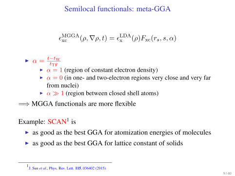
Semilocal functionals: meta-GGA

ǫMGGAxc (ρ,∇ρ, t) = ǫLDA

x (ρ)Fxc(rs, s, α)

◮ α = t−tWtTF

◮ α = 1 (region of constant electron density)◮ α = 0 (in one- and two-electron regions very close and very far

from nuclei)◮ α≫ 1 (region between closed shell atoms)

=⇒ MGGA functionals are more flexible

Example: SCAN1 is

◮ as good as the best GGA for atomization energies of molecules

◮ as good as the best GGA for lattice constant of solids

1J. Sun et al., Phys. Rev. Lett. 115, 036402 (2015)

9 / 40

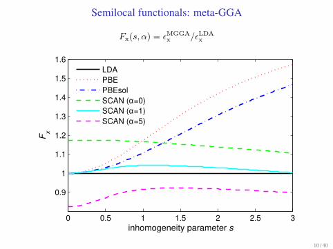
Semilocal functionals: meta-GGA

Fx(s, α) = ǫMGGA

x /ǫLDA

x

0 0.5 1 1.5 2 2.5 3

0.9

1

1.1

1.2

1.3

1.4

1.5

1.6

inhomogeneity parameter s

Fx

LDAPBEPBEsolSCAN (α=0)SCAN (α=1)SCAN (α=5)

10 / 40

Semilocal functionals: MGGA MS2 and SCANTest of functionals on 44 solids1

0 0.5 1 1.5 20

2

4

6

8

PBE

WC

PBEsol

PBEint

PBEalpha

RGE2

SG4

MGGA_MS2 SCAN

Mean absolute percentage error for lattice constant

Mea

n ab

solu

te p

erce

ntag

e er

ror

for

cohe

sive

ene

rgy

• The accurate GGA for solids (cohesive energy/lattice constant). They are ALL very inaccurate for the atomization of molecules

• MGGA_MS2 and SCAN are very accurate for the atomization of molecules

1F. Tran et al., J. Chem. Phys. 144, 204120 (2016)

11 / 40

Input file case.in0: keywords for the xc-functional

The functional is specified at the 1st line of case.in0. Three different

ways:

1. Specify a global keyword for Ex, Ec, vx, vc:◮ TOT XC NAME

2. Specify a keyword for Ex, Ec, vx, vc individually:

◮ TOT EX NAME1 EC NAME2 VX NAME3 VC NAME4

3. Specify keywords to use functionals from Libxc1:

◮ TOT XC TYPE X NAME1 XC TYPE C NAME2

◮ TOT XC TYPE XC NAME

where TYPE is the family name: LDA, GGA or MGGA

1M. A. L. Marques et al., Comput. Phys. Commun. 183, 2272 (2012); S. Lehtola et al., SoftwareX 7, 1 (2018)

http://www.tddft.org/programs/octopus/wiki/index.php/Libxc

12 / 40

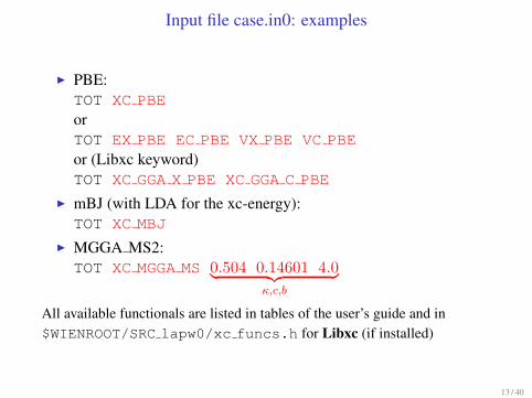
Input file case.in0: examples

◮ PBE:

TOT XC PBE

or

TOT EX PBE EC PBE VX PBE VC PBE

or (Libxc keyword)

TOT XC GGA X PBE XC GGA C PBE

◮ mBJ (with LDA for the xc-energy):

TOT XC MBJ

◮ MGGA MS2:

TOT XC MGGA MS 0.504 0.14601 4.0︸ ︷︷ ︸

κ,c,b

All available functionals are listed in tables of the user’s guide and in

$WIENROOT/SRC lapw0/xc funcs.h for Libxc (if installed)

13 / 40

Methods for van der Waals systems

Problem with semilocal and hybrid functionals:

◮ They do not include London dispersion interactions =⇒ Results

are very often qualitatively wrong for van der Waals systems

Two types of dispersion terms added to the DFT total energy:

◮ Pairwise term (cheap)1:

EPWc,disp = −

∑

A<B

∑

n=6,8,10,...

fdampn (RAB)

CABnRnAB

◮ Nonlocal term (more expensive than semilocal)2:

ENLc,disp =

1

2

∫ ∫

ρ(r1)Φ(r1, r2)ρ(r2)d3r1d

3r2

1S. Grimme, J. Comput. Chem. 25, 1463 (2004)

2M. Dion et al., Phys. Rev. Lett. 92, 246401 (2004)

14 / 40

DFT-D3 pairwise method1

◮ Features:

◮ Cheap◮ CAB

n depend on positions of the nuclei (via coordination number)◮ Energy and forces (minimization of internal parameters)◮ 3-body term available (more important for solids than molecules)

◮ Installation:

◮ Not included in WIEN2k◮ Download and compile the DFTD3 package from

https://www.chemie.uni-bonn.de/pctc/mulliken-center/software/dft-d3/

copy the dftd3 executable in $WIENROOT

◮ Usage:

◮ Input file case.indftd3 (if not present a default one is copied automatically

by x lapw)◮ run(sp) lapw -dftd3 . . .◮ case.scfdftd3 is included in case.scf

1S. Grimme et al., J. Chem. Phys. 132, 154104 (2010)

15 / 40

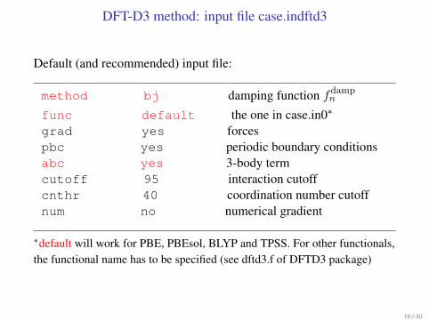
DFT-D3 method: input file case.indftd3

Default (and recommended) input file:

method bj damping function fdampn

func default the one in case.in0∗

grad yes forces

pbc yes periodic boundary conditions

abc yes 3-body term

cutoff 95 interaction cutoff

cnthr 40 coordination number cutoff

num no numerical gradient

∗default will work for PBE, PBEsol, BLYP and TPSS. For other functionals,

the functional name has to be specified (see dftd3.f of DFTD3 package)

16 / 40

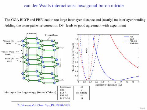
van der Waals interactions: hexagonal boron nitride

The GGA BLYP and PBE lead to too large interlayer distance and (nearly) no interlayer bonding

Adding the atom-pairwise correction D31 leads to good agreement with experiment

3 3.2 3.4 3.6 3.8 4 4.2 4.4 4.6 4.8 50

0.2

0.4

0.6

0.8

1

1.2

1.4

1.6

1.8

2

exp

Interlayer distance (A)

Tota

len

ergy

(mR

y/ce

ll)

PBEBLYPPBE+D3BLYP+D3

Interlayer binding energy (in meV/atom):

Experiment 40

PBE 2

BLYP No binding

PBE-D3 41

BLYP-D3 58

1S. Grimme et al., J. Chem. Phys. 132, 154104 (2010)

17 / 40

Nonlocal vdW functionals

ENLc,disp =

1

2

∫ ∫

ρ(r1)Φ(r1, r2)ρ(r2)d3r1d

3r2

Kernels Φ proposed in the literature:

◮ DRSLL1 (vdW-DF1, optB88-vdW, vdW-DF-cx0, . . . ):

◮ Derived from ACFDT◮ Contains no adjustable parameter

◮ LMKLL2 (vdW-DF2, rev-vdW-DF2):

◮ Zab in DRSLL multiplied by 2.222

◮ rVV103,4:

◮ Different analytical form as DRSLL◮ Parameters: b = 6.3 and C = 0.0093

◮ rVV10L5:

◮ Parameters: b = 10.0 and C = 0.0093◮ DADE5 (not tested on solids):1

M. Dion et al., Phys. Rev. Lett. 92, 246401 (2004)2

K. Lee et al., Phys. Rev. B 82, 081101(R) (2010)3

O. A. Vydrov and T. Van Voorhis, J. Chem. Phys. 133, 244103 (2010)4

R. Sabatini et al., Phys. Rev. B 87, 041108(R) (2013)5

H. Peng and J. P. Perdew, Phys. Rev. B 95, 081105(R) (2017)6

M. Shahbaz and K. Szalewicz, Phys. Rev. Lett 122, 213001 (2019)

18 / 40

Nonlocal vdW functionals in WIEN2k1

◮ Features:

◮ Use the fast FFT-based method of Roman-Perez and Soler2:

1. ρ is smoothed close to the nuclei (density cutoff ρc) → ρs. The

smaller ρc is, the smoother ρs is.

2. ρs is expanded in plane waves in the whole unit cell.

Gmax is the plane-wave cutoff of the expansion.

◮ Many of the vdW functionals from the literature are available (see

user’s guide)

◮ Usage:

◮ Input file case.innlvdw ($WIENROOT/SRC templates)◮ run(sp) lapw -nlvdw . . .◮ case.scfnlvdw is included in case.scf

1F. Tran et al., Phys. Rev. B 96, 054103 (2017)

2G. Roman-Perez and J. M. Soler, Phys. Rev. Lett. 103, 096102 (2009)

19 / 40

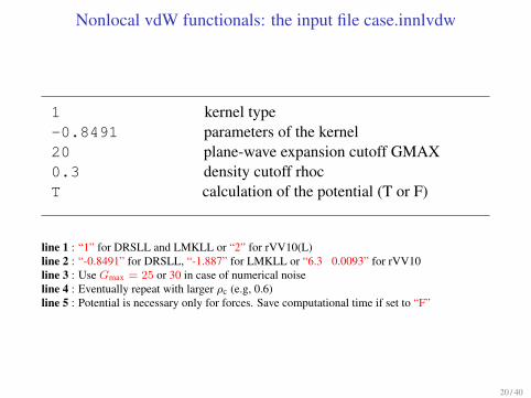
Nonlocal vdW functionals: the input file case.innlvdw

1 kernel type

-0.8491 parameters of the kernel

20 plane-wave expansion cutoff GMAX

0.3 density cutoff rhoc

T calculation of the potential (T or F)

line 1 : “1” for DRSLL and LMKLL or “2” for rVV10(L)

line 2 : “-0.8491” for DRSLL, “-1.887” for LMKLL or “6.3 0.0093” for rVV10

line 3 : Use Gmax = 25 or 30 in case of numerical noise

line 4 : Eventually repeat with larger ρc (e.g, 0.6)

line 5 : Potential is necessary only for forces. Save computational time if set to “F”

20 / 40

van der Waals interactions: tests on solids1

44 strongly bound solids 17 weakly bound solids

0 0.5 1 1.5 2 2.5 3 3.50

2

4

6

8

10

12

14

16

18

(a)

MARE for lattice constant (%)

MA

RE

for

bin

din

gen

ergy

(%)

LDAPBEPBEsolSCANTMvdW−DFvdW−DF2C09−vdWoptB88−vdWoptB86b−vdWrev−vdW−DF2vdW−DF−cxrVV10PBE+rVV10LSCAN+rVV10PBEsol+rVV10sPBE−D3(BJ)revPBE−D3(BJ)

0 1 2 3 4 5 6 70

10

20

30

40

50

60

70

80

90

PBE → (15,81)(b)

MARE for lattice constant (%)

MA

RE

for

bin

din

gen

ergy

(%)

Conclusion: rev-vdW-DF22 is the best functional for solids

1F. Tran et al., Phys. Rev. Materials 3, 063602 (2019)

2I. Hamada, Phys. Rev. B. 89, 121103(R) (2014)

21 / 40

Accurate band gaps with DFT: the modified Becke-Johnson potential

◮ Standard LDA and GGA functionals underestimate the band gap

◮ Hybrid and GW are much more accurate, but also much more

expensive

◮ A cheap alternative is to use the modified Becke-Johnson (mBJ)

potential:1

vmBJ

x (r) = cvBR

x (r) + (3c− 2)1

π

√

5

6

√

t(r)

ρ(r)

where vBRx is the Becke-Roussel potential, t is the kinetic-energy

density and c is given by

c = α+ β

1

Vcell

∫

cell

|∇ρ(r)|

ρ(r)d3r

1/2

mBJ is a MGGA potential

1F. Tran and P. Blaha, Phys. Rev. Lett. 102, 226401 (2009)

22 / 40

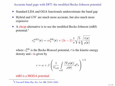
Accurate band gaps with DFT: the modified Becke-Johnson potential

◮ Standard LDA and GGA functionals underestimate the band gap

◮ Hybrid and GW are much more accurate, but also much more

expensive

◮ A cheap alternative is to use the modified Becke-Johnson (mBJ)

potential:1

vmBJ

x (r) = cvBR

x (r) + (3c− 2)1

π

√

5

6

√

t(r)

ρ(r)

where vBRx is the Becke-Roussel potential, t is the kinetic-energy

density and c is given by

c = α+ β

1

Vcell

∫

cell

|∇ρ(r)|

ρ(r)d3r

1/2

mBJ is a MGGA potential

1F. Tran and P. Blaha, Phys. Rev. Lett. 102, 226401 (2009)

22 / 40

Band gaps with mBJ: Reach the GW accuracy

0 2 4 6 8 10 12 14 16

0

2

4

6

8

10

12

14

16

Experimental band gap (eV)

The

oret

ical

ban

d ga

p (

eV)

Ar

Kr

Xe

C

Si

G

e

LiF

LiC

l

MgO

ScN

MnO

FeO

NiO

SiC

BN

GaN

GaA

s

AlP

ZnS

CdS

A

lN

ZnO

LDAmBJHSEG

0W

0

GW

See also F. Tran and P. Blaha, J. Phys. Chem. A 121, 3318 (2017) (76 solids)

P. Borlido et al., J. Chem. Theory Comput. xx, xxxx (2019) (472 solids)23 / 40

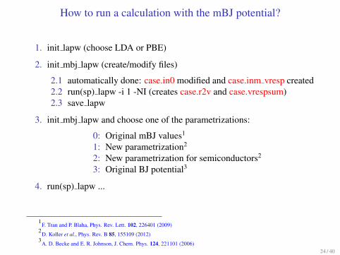
How to run a calculation with the mBJ potential?

1. init lapw (choose LDA or PBE)

2. init mbj lapw (create/modify files)

2.1 automatically done: case.in0 modified and case.inm vresp created

2.2 run(sp) lapw -i 1 -NI (creates case.r2v and case.vrespsum)

2.3 save lapw

3. init mbj lapw and choose one of the parametrizations:

0: Original mBJ values1

1: New parametrization2

2: New parametrization for semiconductors2

3: Original BJ potential3

4. run(sp) lapw ...

1F. Tran and P. Blaha, Phys. Rev. Lett. 102, 226401 (2009)

2D. Koller et al., Phys. Rev. B 85, 155109 (2012)

3A. D. Becke and E. R. Johnson, J. Chem. Phys. 124, 221101 (2006)

24 / 40

GLLB-SC potential for band gaps

◮ GLLB-SC is a potential (no energy functional)1:

vGLLB-SCxc,σ = 2εPBEsol

x,σ +KLDAx

Nσ∑

i=1

√ǫH − ǫiσ

|ψiσ |2

ρσ+ vPBEsol

c,σ

◮ Leads to an derivative discontinuity:

∆ =

∫

ψ∗L

NσL∑

i=1

KLDAx

(√

ǫL − ǫiσL−

√

ǫH − ǫiσL

)

∣

∣ψiσL

∣

∣

2

ρσL

ψLd3r

Comparison with experiment: Eg = EKSg +∆

◮ Much better than LDA/GGA for band gaps

◮ Not as good as mBJ for strongly correlated systems2

◮ Seems interesting for electric field gradient2

◮ See user’s guide for usage

1M. Kuisma et al., Phys. Rev. B 82, 115106 (2010)

1F. Tran, S. Ehsan, and P. Blaha, Phys. Rev. Materials 2, 023802 (2018)

25 / 40

Strongly correlated electrons

Problem with semilocal functionals:

◮ They give qualitatively wrong results for solids which contain

localized 3d or 4f electrons

◮ The band gap is too small (zero in FeO!)◮ The magnetic moment is too small (zero in YBa2Cu3O6!)◮ Wrong electronic configuration

Why?

◮ The strong on-site correlations are not correctly accounted for by

semilocal functionals.

(Partial) solution to the problem:

◮ Combine semilocal functionals with Hartree-Fock theory:

◮ DFT+U◮ Hybrid

Even better:

◮ LDA+DMFT (DMFT codes using WIEN2k orbitals as input

exist)

26 / 40

Strongly correlated electrons

Problem with semilocal functionals:

◮ They give qualitatively wrong results for solids which contain

localized 3d or 4f electrons

◮ The band gap is too small (zero in FeO!)◮ The magnetic moment is too small (zero in YBa2Cu3O6!)◮ Wrong electronic configuration

Why?

◮ The strong on-site correlations are not correctly accounted for by

semilocal functionals.

(Partial) solution to the problem:

◮ Combine semilocal functionals with Hartree-Fock theory:

◮ DFT+U◮ Hybrid

Even better:

◮ LDA+DMFT (DMFT codes using WIEN2k orbitals as input

exist)

26 / 40

Strongly correlated electrons

Problem with semilocal functionals:

◮ They give qualitatively wrong results for solids which contain

localized 3d or 4f electrons

◮ The band gap is too small (zero in FeO!)◮ The magnetic moment is too small (zero in YBa2Cu3O6!)◮ Wrong electronic configuration

Why?

◮ The strong on-site correlations are not correctly accounted for by

semilocal functionals.

(Partial) solution to the problem:

◮ Combine semilocal functionals with Hartree-Fock theory:

◮ DFT+U◮ Hybrid

Even better:

◮ LDA+DMFT (DMFT codes using WIEN2k orbitals as input

exist)

26 / 40

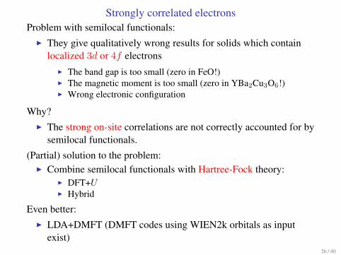
Strongly correlated electrons

Problem with semilocal functionals:

◮ They give qualitatively wrong results for solids which contain

localized 3d or 4f electrons

◮ The band gap is too small (zero in FeO!)◮ The magnetic moment is too small (zero in YBa2Cu3O6!)◮ Wrong electronic configuration

Why?

◮ The strong on-site correlations are not correctly accounted for by

semilocal functionals.

(Partial) solution to the problem:

◮ Combine semilocal functionals with Hartree-Fock theory:

◮ DFT+U◮ Hybrid

Even better:

◮ LDA+DMFT (DMFT codes using WIEN2k orbitals as input

exist)

26 / 40

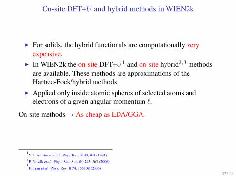
On-site DFT+U and hybrid methods in WIEN2k

◮ For solids, the hybrid functionals are computationally very

expensive.

◮ In WIEN2k the on-site DFT+U 1 and on-site hybrid2,3 methods

are available. These methods are approximations of the

Hartree-Fock/hybrid methods

◮ Applied only inside atomic spheres of selected atoms and

electrons of a given angular momentum ℓ.

On-site methods → As cheap as LDA/GGA.

1V. I. Anisimov et al., Phys. Rev. B 44, 943 (1991)

2P. Novak et al., Phys. Stat. Sol. (b) 243, 563 (2006)

3F. Tran et al., Phys. Rev. B 74, 155108 (2006)

27 / 40

DFT+U and hybrid exchange-correlation functionals

The exchange-correlation functional is

EDFT+U/hybridxc = EDFT

xc [ρ] + Eonsite[nmm′ ]

where nmm′ is the density matrix of the correlated electrons

◮ For DFT+U both exchange and Coulomb are corrected:

Eonsite = EHFx + ECoul

︸ ︷︷ ︸

correction

−EDFTx − EDFT

Coul︸ ︷︷ ︸

double counting

There are several versions of the double-counting term

◮ For the hybrid methods only exchange is corrected:

Eonsite = αEHFx

︸ ︷︷ ︸

corr.

−αELDAx

︸ ︷︷ ︸

d. count.

where α is a parameter ∈ [0, 1]

28 / 40

How to run DFT+U and on-site hybrid calculations?

1. Create the input files:

◮ case.inorb and case.indm for DFT+U◮ case.ineece for on-site hybrid functionals (case.indm created

automatically):

2. Run the job (can only be run with runsp lapw):

◮ LDA+U : runsp lapw -orb . . .◮ Hybrid: runsp lapw -eece . . .

For a calculation without spin-polarization (ρ↑ = ρ↓):

runsp c lapw -orb/eece . . .

29 / 40

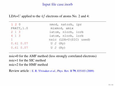
Input file case.inorb

LDA+U applied to the 4f electrons of atoms No. 2 and 4:

1 2 0 nmod, natorb, ipr

PRATT,1.0 mixmod, amix

2 1 3 iatom, nlorb, lorb

4 1 3 iatom, nlorb, lorb

1 nsic (LDA+U(SIC) used)

0.61 0.07 U J (Ry)

0.61 0.07 U J (Ry)

nsic=0 for the AMF method (less strongly correlated electrons)

nsic=1 for the SIC method

nsic=2 for the HMF method

Review article : E. R. Ylvisaker et al., Phys. Rev. B 79, 035103 (2009)

30 / 40

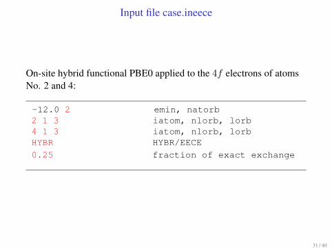
Input file case.ineece

On-site hybrid functional PBE0 applied to the 4f electrons of atoms

No. 2 and 4:

-12.0 2 emin, natorb

2 1 3 iatom, nlorb, lorb

4 1 3 iatom, nlorb, lorb

HYBR HYBR/EECE

0.25 fraction of exact exchange

31 / 40

SCF cycle of DFT+U in WIEN2k

lapw0 → vDFTxc,σ + vee + ven (case.vspup(dn), case.vnsup(dn))

orb -up → v↑mm′ (case.vorbup)

orb -dn → v↓mm′ (case.vorbdn)

lapw1 -up -orb → ψ↑nk, ǫ↑nk

(case.vectorup, case.energyup)

lapw1 -dn -orb → ψ↓nk, ǫ↓nk

(case.vectordn, case.energydn)

lapw2 -up -orb → ρ↑val

(case.clmvalup), n↑mm′ (case.dmatup)

lapw2 -dn -orb → ρ↓val

(case.clmvaldn), n↓mm′ (case.dmatdn)

lcore -up → ρ↑core (case.clmcorup)

lcore -dn → ρ↓core (case.clmcordn)

mixer → mixed ρσ and nσmm′

32 / 40

Hybrid functionals

◮ On-site hybrid functionals can be applied only to localized electrons

◮ Full hybrid functionals are necessary (but expensive) for solids with

delocalized electrons (e.g., in sp-semiconductors)

Two types of full hybrid functionals available in WIEN2k1:

◮ unscreened:

Exc = EDFT

xc + α(

EHF

x − EDFT

x

)

◮ screened (short-range), 1

|r−r′|→ e

−λ|r−r′||r−r′|

:

Exc = EDFT

xc + α(

ESR−HF

x − ESR−DFT

x

)

screening leads to faster convergence with k-points sampling

1F. Tran and P. Blaha, Phys. Rev. B 83, 235118 (2011)

33 / 40

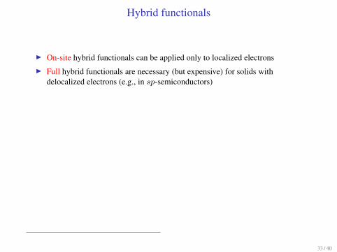
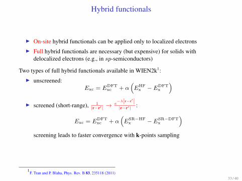
Hybrid functionals

◮ On-site hybrid functionals can be applied only to localized electrons

◮ Full hybrid functionals are necessary (but expensive) for solids with

delocalized electrons (e.g., in sp-semiconductors)

Two types of full hybrid functionals available in WIEN2k1:

◮ unscreened:

Exc = EDFT

xc + α(

EHF

x − EDFT

x

)

◮ screened (short-range), 1

|r−r′|→ e

−λ|r−r′||r−r′|

:

Exc = EDFT

xc + α(

ESR−HF

x − ESR−DFT

x

)

screening leads to faster convergence with k-points sampling

1F. Tran and P. Blaha, Phys. Rev. B 83, 235118 (2011)

33 / 40

Hybrid functionals: technical details

◮ 10-1000 times more expensive than LDA/GGA

◮ k-point and MPI parallelization

◮ Approximations to speed up the calculations:

◮ Reduced k-mesh for the HF potential. Example:

For a calculation with a 12× 12× 12 k-mesh, the reduced k-mesh for

the HF potential can be:

6× 6× 6, 4× 4× 4, 3× 3× 3, 2× 2× 2 or 1× 1× 1◮ Non-self-consistent calculation of the band structure

◮ Underlying functionals for unscreened and screened hybrid:

◮ LDA, PBE, WC, PBEsol, B3PW91, B3LYP

◮ Use run bandplothf lapw for band structure

◮ Can be combined with spin-orbit coupling

34 / 40

Hybrid functionals: input file case.inhf

Example for YS-PBE0 (similar to HSE06 from Heyd, Scuseria and Ernzerhof1)

0.25 fraction α of HF exchange

T screened (T, YS-PBE0) or unscreened (F, PBE0)

0.165 screening parameter λ20 number of bands for the 2nd Hamiltonian

6 GMAX

3 lmax for the expansion of orbitals

3 lmax for the product of two orbitals

1d-3 radial integrals below this value neglected

Important: The computational time will depend strongly on the

number of bands, GMAX, lmax and the number of k-points

1A. V. Krukau et al., J. Chem. Phys. 125, 224106 (2006)

35 / 40

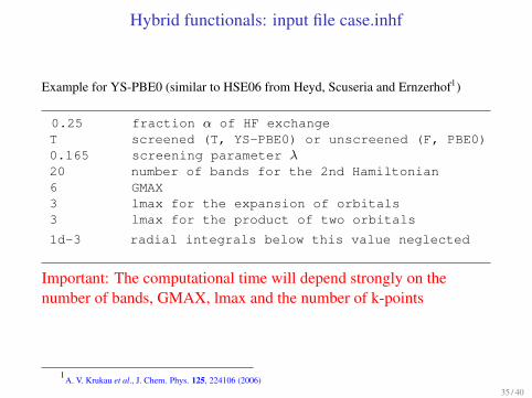
Hybrid functionals: input file case.inhf

Example for YS-PBE0 (similar to HSE06 from Heyd, Scuseria and Ernzerhof1)

0.25 fraction α of HF exchange

T screened (T, YS-PBE0) or unscreened (F, PBE0)

0.165 screening parameter λ20 number of bands for the 2nd Hamiltonian

6 GMAX

3 lmax for the expansion of orbitals

3 lmax for the product of two orbitals

1d-3 radial integrals below this value neglected

Important: The computational time will depend strongly on the

number of bands, GMAX, lmax and the number of k-points

1A. V. Krukau et al., J. Chem. Phys. 125, 224106 (2006)

35 / 40

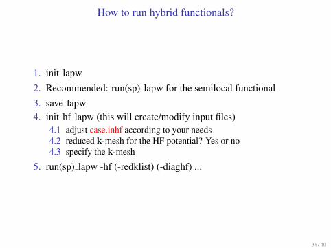
How to run hybrid functionals?

1. init lapw

2. Recommended: run(sp) lapw for the semilocal functional

3. save lapw

4. init hf lapw (this will create/modify input files)

4.1 adjust case.inhf according to your needs

4.2 reduced k-mesh for the HF potential? Yes or no

4.3 specify the k-mesh

5. run(sp) lapw -hf (-redklist) (-diaghf) ...

36 / 40

SCF cycle of hybrid functionals in WIEN2k

lapw0 -grr → vDFTx (case.r2v), αEDFT

x (:AEXSL)

lapw0 → vDFTxc + vee + ven (case.vsp, case.vns)

lapw1 → ψDFTnk , ǫDFT

nk (case.vector, case.energy)

lapw2 →∑

nk ǫDFTnk (:SLSUM)

hf → ψnk, ǫnk (case.vectorhf, case.energyhf)

lapw2 -hf → ρval (case.clmval)

lcore → ρcore (case.clmcor)

mixer → mixed ρ

37 / 40

Nonmagnetic and ferromagnetic phases of cerium1

Small U (1.5 eV) or αx (0.08) leads to correct stability ordering

4.3 4.4 4.5 4.6 4.7 4.8 4.9 5 5.1 5.2 5.3 5.4 5.5 5.60

100

200

300

400

500T

otal

ene

rgy

(m

eV)

PBE

FMNM

4.3 4.4 4.5 4.6 4.7 4.8 4.9 5 5.1 5.2 5.3 5.4 5.5 5.60

25

50

75

100

125

150

Tot

al e

nerg

y (

meV

)

PBE+U (U=1.5 eV)

FM1NM

4.3 4.4 4.5 4.6 4.7 4.8 4.9 5 5.1 5.2 5.3 5.4 5.5 5.60

200

400

600

800

1000

Lattice constant (Å)

Tot

al e

nerg

y (

meV

)

PBE+U (U=4.3 eV)

FM2NM

4.3 4.4 4.5 4.6 4.7 4.8 4.9 5 5.1 5.2 5.3 5.4 5.5 5.60

100

200

300

400

500

Tot

al e

nerg

y (

meV

)

PBE

FMNM

4.3 4.4 4.5 4.6 4.7 4.8 4.9 5 5.1 5.2 5.3 5.4 5.5 5.60

25

50

75

100

125

150

Tot

al e

nerg

y (

meV

)

YS−PBEh (αx=0.08)

FM1NM

4.3 4.4 4.5 4.6 4.7 4.8 4.9 5 5.1 5.2 5.3 5.4 5.5 5.60

100

200

300

400

500

600

700

Lattice constant (Å)

Tot

al e

nerg

y (

meV

)

YS−PBEh (αx=0.25)

FM1NM

1F. Tran, F. Karsai, and P. Blaha, Phys. Rev. B 89, 155106 (2014)

38 / 40

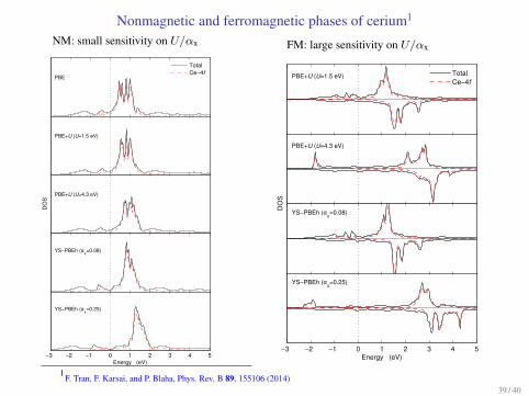
Nonmagnetic and ferromagnetic phases of cerium1

NM: small sensitivity on U/αx

PBE

TotalCe−4f

PBE+U (U=1.5 eV)

PBE+U (U=4.3 eV)

YS−PBEh (αx=0.08)

−3 −2 −1 0 1 2 3 4 5Energy (eV)

YS−PBEh (αx=0.25)

DO

SFM: large sensitivity on U/αx

PBE+U (U=1.5 eV) TotalCe−4f

PBE+U (U=4.3 eV)

YS−PBEh (αx=0.08)

−3 −2 −1 0 1 2 3 4 5Energy (eV)

YS−PBEh (αx=0.25)

DO

S

1F. Tran, F. Karsai, and P. Blaha, Phys. Rev. B 89, 155106 (2014)

39 / 40

Some recommendations

Before using a functional:

◮ read a few papers about the functional in order to know

◮ for which properties or types of solids it is supposed to be reliable◮ if it is adapted to your problem

◮ figure out if you have enough computational ressources

◮ hybrid functionals and GW require (substantially) more

computational ressources (and patience)

40 / 40