Jayeofa F. Opedljl

NJTD <2010> 7(1) 48-

57 Faculty of Engineering & Technology University of llo~~~~ciri~~8~i!:.

SDEVELOPMENT OF A COMPUTER-AIDED LEARNING SYSTEM FOR GRAPHICALANALYSIS OF CONTINUOUS-TIME CONTROL SYSTEMS

JAYEOLA F. OPADIJI Department of Electrical Engineering, University of florin, llorin, Nigeriae­

~-mailjopadiji@unilorin.edu.ng

· ABSTRACT . We prese.nt the development and deployment process of a computer-aided learning tool which serves as a training aid for undergraduate control engineering courses. We.show the process of aigorithm construction ~nd

. implementation of the=software which ·is also aimed at teaching software- -•. de\(elopment at undergraduate level. The scope of this. project is limited to ·· . · g.raphical:analysis of continuous-time control systems~ · ·

:: Keywords: Simulation, Computer-aided learning, Continuous-time control · system

1.0 INTRODUCTION In recent years, there ·.

has been a shortfall in the ···number of students offering to

: . option in~ -the field . of Control · Engineering_ at undergraduate

level in Nigerian universities. In fact, this ha~- been so dramatic that, some universities no longer offer the-discipline as an option in .th~ Electrical and Electronic departments. When investigated, if was found out that, a number of reasons have contributed to this, but prominent among. these are the

. fa~ that, there are not enough ·teaching ~nd laboratory materials · to -assist in the disseminating Qf knowledge in this field.Also, there has been a great drop. in· teaching personnel who · specialize in Control Engineering {Nwadiani Nigeria Journal of Technofoglcal Developfl'\8nt

·this field. Also, there has. ·been a . great drop in teaching personnel­wh o specialize in Control Engineering (Nwadiani and .Apotu, 200Z; Oni, 1999). It is

· against· this backdrop tliat this prQject was initiated; .to~provide a software teaching aid for the introduction of students to the field

· of control engineering.However,_ it was discovered that software liKe this will not only serve· as a · teaching aid for control

. engineering students but also aid · in teaching engineering students

some funaamental pnnciples of computer programming~ The . factors mentioned above served as tools in desi.g_ning. the scope and objectives oflhis work.

Control Engineering is a field of study, which cuts across every area of human existence. It invorves the use of available resources to cause a system to behave in a predetermined manner based on information obtained about the system. The-­evolution. of Control Eng_ineering practice has brought with it; the mtroduction of complex anal~ical tools for the purpose of modelling

· and P.redicting systems whose behaviour would of course have to be understood before they can be controlled. .

48 Volume7 (1) 2010 .

. ·,

. Jayeola F. Opadljl ISSN: 0189-9546 NJTD (2010) 7(1) 48- 57 Faculty of Engineering & Technology University of llorln, llorin, Nigeria.

.. In ·developing any system.. 2.0 PROJECT OBJECTIVE . time always happens to be a major . There were two main constraint, therefore, the use of objectives of this· software complex graphical and mathematical · d I t · ct d th tools, which · require long hours Qf eve opmen proje an ese ·manual implementation may not b~ ~re enumerated oelow: . . appropriate~ Before any accurate plot·. (1.) __ T~~ development of su.1table can be done manuallYi it is required algorathms for . analysis .·of that a table o( values ,;.ust be gotten . systems defined in the scope of and this could be · very tedious· the project.work .. especially for high-order syste'!1s· · (ii.) The. implementation of the · · ~urth~rmore, the P~ of p~ng developed algorithms using an 1~elf 1s e~erg.y sappin~ if the pomts appropriate .proQr~m.mi~g_

.·~re many. Us1~g_ machmes however, language that will aid m 1s not automatic, as they have to be . . . f . instructed in .what to do in the form of t e a c h I n g s o t Vt! a r e programmes written to perform development. · · specific tasks. Algorithms have to be These objectives wete set with developed for any of the analytical due consideration_ .of the target tools b~fore they can ',be users. of the computer implemented. _ · . programs.

·Thus, this is the first hurdle to . · be crossed In the development of 3.~ Sys~ Design and Algorithm Development . approp.riate software. The · ·· implementation of these algorithms is ·also a task to be· accomplished, . paying . full attention to software development principles (Aho,

···:.Hopcroftand Ullman, 1974; Brassard : · .. and Bralley, 1996) Fl;lnt Mod:lllr~o1111oeor-.&tmm

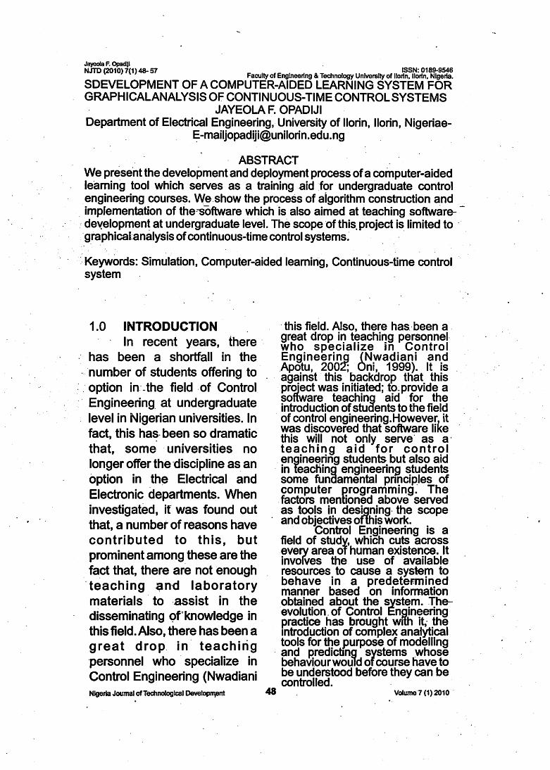
The scope of the project work · - · A modular approach was covers .graphical_ ~~alytical · tools employed at the design stage of · · used rn class.1cal co~trol the software (Aptech, 1999). · systems:Time response graph . The first step taken was to

·(i.)Rootlocus ~reak the whole system down · .. . · · anto modules and each module (11.)Nyq.u1st ~lot was then developed separately · (lii.)Bode plot before.final integration to form a (iv.)Nicholsplot. whole system as shown in the

The above tools were implemented in a computer software environment for the analysis of .continuous-time control systems.

Nigeria Jownal of Technological Development

modular plan of the whole system. Figure 1 shows a modular plan of the whole system. Each module was · further broken down into three segments as explained below:

49 Vorume 7 (1) 2010

·.

Jayeola F. Opad!jl NJTD (2010) 7(1) 48-57

3.1 The Input Interface: The input interfaces were

designed to receive system parameters as designed for in the algorithms developed. These interfaces were· designed to trap errors in data entry so. that user · will be guided as to which data are.· valid for the different syst~m parameters us~d as inputS .

. 3.2 The Processing Engine:· ·· · ·This" sub-moduJe is

responsible ·for carrying out · specified operations on the i~put . parameters as laid out in the developed algorithm for that .

. module. The results. of these · · operations are sent to the output

interface for display.

. 3.3 · . The Output Interface: Each output interface is

made up of the graph section as .well as the performance parameter section. Results gotten from the processing sub-module are displayed in this interface.

·. 4.0 . ALGORITHMDEVELOPMENT:

Algorithms were designed for the five modules. of the project. In developing the algorithms. adequate attention was paid to coniputat?ilil¥ of each of the steps · since the computer requires that each step must not be ambiguous. Moreover, the algorithms are meant to be used for the purpose of teaching. programming to students. ·

Nigeria Journal of Technological Development

ISSN: 0189-9546 Faculty of Engineering & Technology University of llorln, llorln, Nigeria.

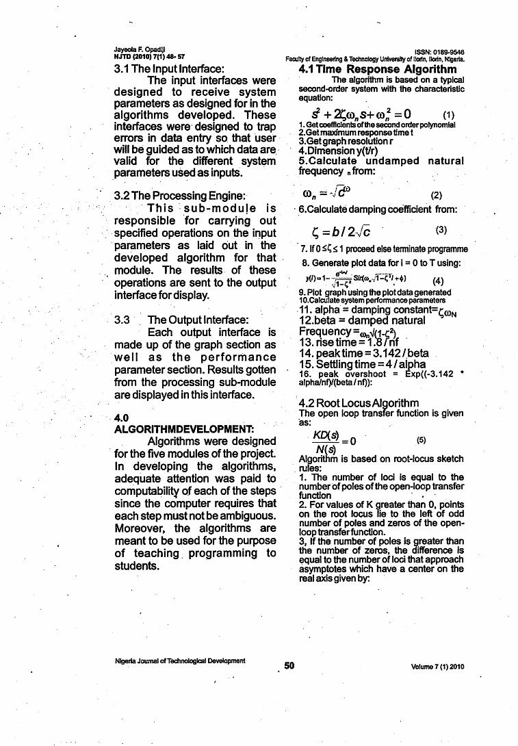
4.1 Time Response Algorithm The algorithm is based on a typical

second-order system with the characteristic equation:

s +~wns+ro; =0 (1) 1. Get coefficients of the second orderpolynomfal 2.Get maximum response time t 3.Get graph resolution r 4.Dimension y(t/r) 5.Calculate undamped natural ,frequency n from: .

(2)

. · _6.Calculate damping coefficient from:

.c; =bl 2 . .1-c · <3> 7. If 0 ~~ s 1 proceed else terminate programme 8. Generate plot data for i = 0 to T using:

}'(/)"" 1--~ .. .:. S/r(co .Jf.::.(f/ + +) . .,;1-1;2 ,, ' • (4)

9. Plot graph using the plot data generated 10.Calculate system perfonnance parameters .11. alpha·= damping constant=t;roN 12.beta = damped natural Frequency =m,;-Jc1-c2) 13. rise time= 1.8fnf · 14. peak time= 3.142/.beta 15. Settling time= 41 alpha 16. peak overshoot = Exp((-3.142 * alpha/nf)/(beta Inf)):

· 4.2 Root Locus Algorithm The open loop transfer function is given ·as:

. KD<.s) = 0 cs> N(s)

Algorithm is based on root-locus sketch · rules:

50

1. The number of loci is equal to the number of poles of the open-loop transfer function · • 2. For values of K greater than 0, points on the root locus lie to the left of odd number of poles and zeros of the open­loop transfer function. 3, If the number of poles is greater than the number of zeros, the difference is equal to the number of loci that approach asymptotes which have a center on the real axis given by: ·

Vofume 7 (1) 2010

Jayeola F. Opadijl NJTO (2010) 7(1) 48- 57

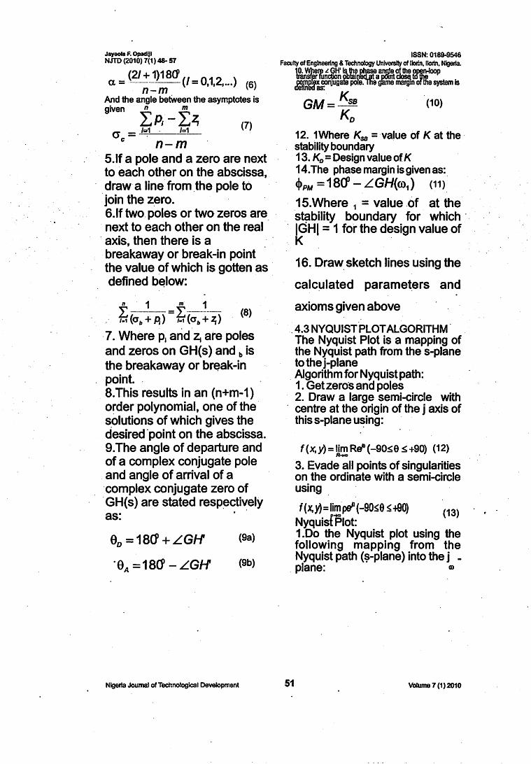
a= {?I +_))18<1(/=0,1,2, ... ) (6) n-m

And the angle betWeen the asymptotes is given n m

LP, - Li; O' = '=:1 . /=1

c n-m (7)

5.lf a pole and a zero are next to each other on the abscissa, draw a line from _the pole to ·join the z~ro. 6.lf two. poles or two zeros are_

· next to each other on the real · axis, then there is a · breakaway or break-in point the value of which is gotten as · defined b~low:

n 1 m· 1 . · ~{a:·+-A) = f.; (~~··+···~") (B)

· 7. Where p1 arid z ate poles and zeros on GH(s) and bis the breakaway or break-in point. . 8. This results in an (n+m-1) order polynomial, one of the· solutions of which gives the desired ·point on the abscissa. 9.The angle of departure and of a complex conjugate pole

. and angle of arrival of a ·complex conjugate zero of · GH(s) are stated resp~cti~ely as:

00 =1ao> + LGH <9a>

·9A =18Q> - LGH (eb)

Nigeria Journal of Technologlcal Development

ISSN: 0189-9546 Faculty of Engineering & Technology UnfvefSlty of llorfn. Clorln. Nigeria.

ge'Jli L GH'. ~tfre!l8!8 ~m'.\\ ~ PJ>!ftlooP creimif ~~'fuGare po~e 8gini8 marg1norBie system is

GM= KS£! (10)

Ko 12. 1Where Kss =·value of Kat the· stability boundary 13. K0 = Design value of K 14. The phase margin is given as: <i>PM =18o>- LGH(ro1) (11).

15. Where 1 = value of . at the ·s~bility boundary for which ·.

· IGHI = 1 for the design value of K .

16. Draw_ sketch lines using the

calc~lated paramet_ers and

axioms given above

. 4.3 NYQUIST PLOT ALGORITHM The Nyquist Plot is a mapping of the Nyquist path from the s-plane to the j-plane

. Algorithm for Nyquist path: 1. Get zeros and poles 2. Draw a large semi-circle with

· centre at the origin of the j axis of this s-plane u~ing:

f(x,y)= lim R~(-90sa s+90) (12) R-.-o

3. Evade all points of singularities on the ordinate with a semi-circle using .

f (x,y)=lim.pff (-90~0 ~+90) Nyquis{Plot:

(13)

1.Do the Nyquist plot using the following mapping from the Nyquist path (~-plane) into the j -

. plane: m

51 Volume 7 (1) 2010

' .

Jayeola F. Opadijl NJTO (2010) 7(1) 48· 57

2.The limit of the straight line portion on the s-plane is given by S= + jro(O<ro <ro0 ) (14) 3.Wherero. is a point of singularity 4.The limits of the small semi­circle on the ordinate is given by S= lim ~ (-9Cf <0 < +9Cf) · (15a)

p...0

. 5.The limits of the large semi-circle is given by

S= Um REf (-9(11 < e < +9(11) (15b)

6.The limits of the poles on the j _ axis is

s=llr:rt(±jro+Pe'8){-9(11 <0 < +9Cl°) (16) .

4.4 BODE PLOT ALGORITHM The Bode form for the open-loop transfer function used is:

. K(1 + j(J) I z,)(1+ jro I zJ .. (1 + j(J) /Zr:,) jro'(1 + jro / p1)(1+ jro/ p2) ••• (1+ jro/ p.,) (17

)

Where z's and p's are zeros and poles respectively and I is a nonnegative integer 1.Get number poles and zeros 2.Get maximum value of w(max) and resolution r 3.lnitialize i = 1 4.Calculate the dB.value for each term in GH(o1)forro= i 5.Add all the terms to get the dB value for GH(i) 6.Find the phase angle for each term in GH(0) for ro = i 7 .Add all the terms to obtain the phase angle of GH(i) 8. Find the logarithm valu .of ro=I 9. Plot point in step 5 against point in step 8 10. Plot point in step 7 against point in step 8 · 11. Increment i_by r

Nigeria Journal ofTechnologlcal Development

ISSN: 0189-9546 FaaJity of Engineering & Technology Onivenlity of llorln. llorln. Nlgerla.

12.lf I is less than maxgotostep4 13. Terminate run 4.5 NICHOLS CHART PLOT ALGORITHM

The plot is done on a chart made up of constant dB magnitude circle and constant phase angles circles. The constant dB-magnitude circles are gotten from the relation:

2M' M' IGH(m)r+ M' -11GH(m)ICo.!.l + M' - 1=0 (18)

The constant phase angle circles are . go.tten from:

1 · l~(ro )~Cose- N Sine (19)

52

f. Get number poles and zeros · 2. Get maximum value of (max) and resolution r 3. Initialize i = 1 4. Calculate the dB value for each term in GHQfor=i . 5.Aad all the terms to get the dB value for GH(i) 6. Find the phase angle for each term in GH(.) for = i 7. Add all the terms to obtain the phase angle of GH(i) 8.Plot point in step 5 against point in step 9. Increment i by r 10. If i is less than max go to step 4 11. Terminate run

5.0 SYSTEM IMPLEMENTATION The implementation of the

design was done using the Microsoft Visual BASIC 6.0. The choice of this software was necessitated by the need to demonstrate the process of Rapid Application Development (RAD) and also take advantage of its Graphic User Interface (GUI) to produce a user-friendly environment for the software that is being developed. Shown below is the main menu of the developed software and sample results of two of its modules.

· 5.1 . TIME RESPONSE MODULE Oh clicking on the "lime Response" button on the main menu window of figure 2, the main menu window is unloaded and the time response input parameter window pops up as shown in figure3. .

Volume 7 (1) 2010

Joyeola F. Opadljl NJTD (2010) 7(1) 48- 57

HMjtfktfMf1¢tfffi

MAIN MENU '

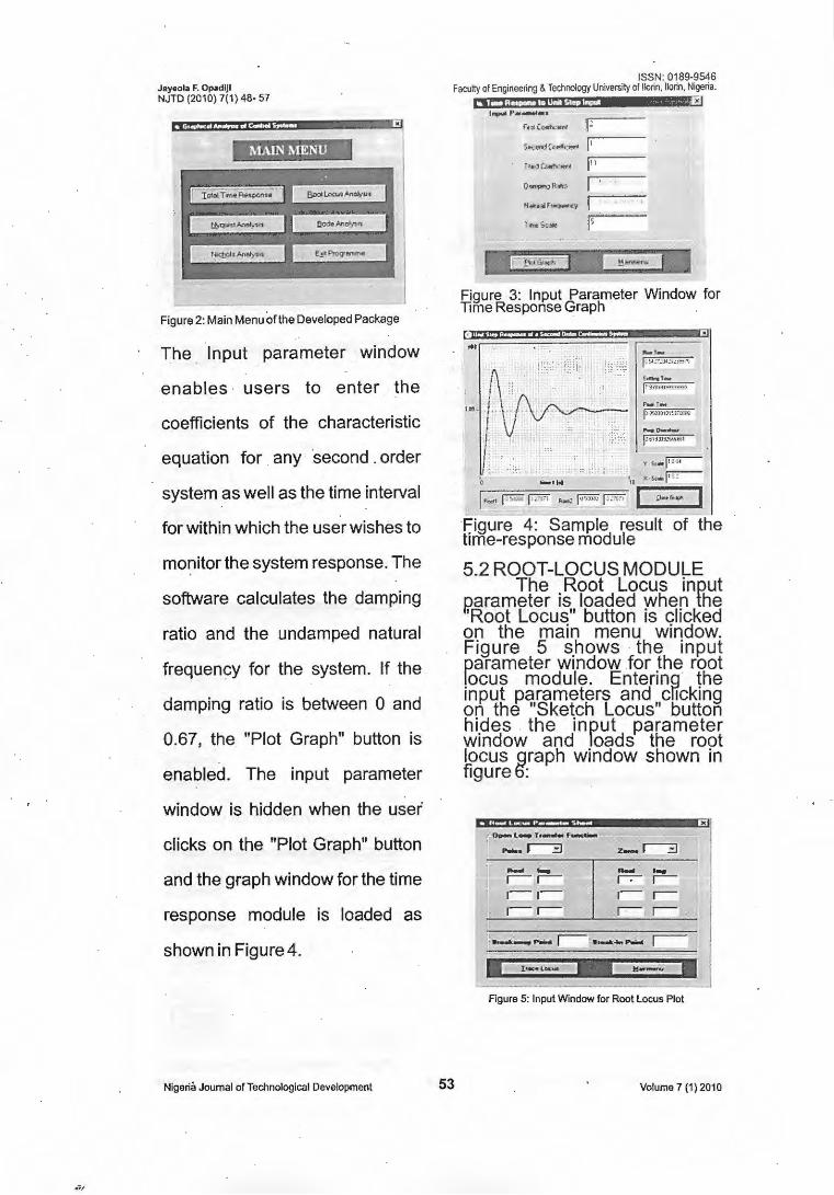
Figure 2: Main Menu of the Developed Package

The Input parameter window

enables · users to enter the

coefficients of the characteristic

equation for any ·second . order

system as well as the time interval

for within which the user wishes to

mo~itorthe system response. The

software calculates the damping

ratio and the undamped natural

frequency for the system. If the

damping ratio is between 0 and

0.67, the "Plot Graph" button is

enabled. The input parameter

window is hidden when the user'

clicks on the "Plot Graph" button

and the graph window for the time

response module is loaded as

shown in Figure 4.

Nigeria Journal of Technological Development

ISSN: 0189-9546 Faculty of Engineering & Technology University of llorin. llorin, Nigeria.

53

, ... ,..,. ,., ......... r • ., Cccth: llff"i I.! s~...i"""'<.,... ~I, ---ft,ijtc;ct..-.,,, p 1

Figure 3: Input Parameter Window for Time Response Graph

( fiifli?@f !i lfHHI• 5; I fj ...

...

... ,_ fJ ~:.•:.Jl.~"vJ. m'">

~1-1 ~..,.,,,,.,.!h ...... ..... _ pJ'~»1J1!muc

Y ·ka~ t •••·:;· I X·Sc-•~ 0 .... ,let 1•---1- iorn P'1 --= fQ%» ~ I ""...... I

Figure 4: Sample result of the time-response module

5.2 ROOT-LOCUS MODULE The Root Locus input

f?iarameter is loaded when the 'Root Locus" button is clicked on the main menu window. Figure 5 shows the input parameter window .for the root locus module. Entering· the input parameters and clicking on the "Sketch Locus" button hides the input parameter window and loads the root locus graph window shown in figure 6:

~... ...... ... r-r- ~ r-r-r- r- r-r-r- ..-- r-

Figure 5: Input Window for Root Locus Plot

Volume 7 (1) 2010

Jayeola F. Opadiji NJTD (2010) 7(1) 48- 57

-·-I ............

Fi I o.-~.~ I

~-------'·---·- it-Locus Plot

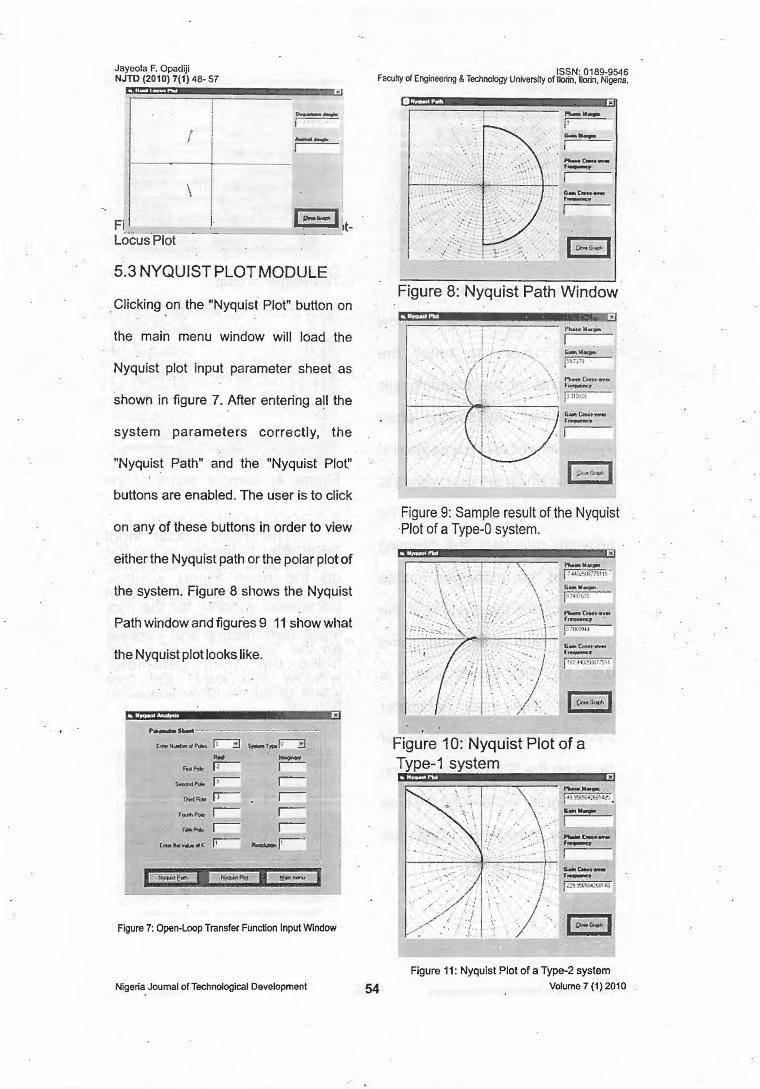
5.3 NYQUIST PLOT MODULE

Clicking on the "Nyquist Plot" button on

the main menu window will load the

Nyquist plot input parameter sheet as

shown in figure 7. After ent~ring a!I the

system parameters correctly, the

"Nyquist Path" and the "Nyquist Plot"

buttons are enabled. The user is to click

on any of these buttons in order to view

either the Nyquist path or the polar plot of

the system. Figure 8 shows the Nyquist

Path window and figures 9 11 show what

the Nyquist plot looks like.

Hdflf , •I

, ........ , ..... l_H_al_ ~ ._, ... ~

Figure 7: Open-Loop Transfer Function Input Window

Nigeria Journal ofTechnological Development

. ISSN: 0189-9546 Faculty of Engineering & Technology Universlly of llorin, llorin, Nigeria.

54

..._ .. _ " .... _

Figure 8: Nyquist Path Window

1--~~~->-•~~~~---,

G.-i w.tt,_

i""'' l'liie.wC..n~ ,_, jJ JHI'..•

Figure 9: Sample result of the Nyquist ·Plot of a Type-0 system.

htifl. PhM•M•ClW' 1 ~ 4~•1t:o()'/W)11~

c-w .... I "' •.

• I

f'tl.tMCt .. , .... ~~ .. j>U»I•

c-c....­r-· 1 · ~:/.l~·w~·n

Figure 10: Nyquist Plot of a Type-1 system

-­P•':"..t''.&_.~£1.> . c ... ....,..

I

Figure 11: Nyquist Plot of a Type-2 system

Volume 7 (1) 2010

Jayeola F. Opadljl NJTD (2010) 7(1) 48- 57

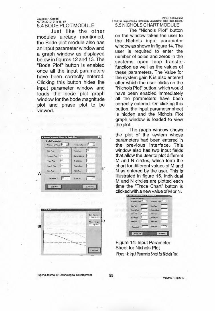
5.4 BODE PLOT MODULE Just like the other

modules alre·ady mentioned, the Bode plot module also has an input parameter window and a graph window as displayed below in figures 12 and 13. The "Bode Plot" button is enabled once all the input parameters have been . correctly entered. Clicking this button hides the

· input parameter window and loads the bode plot graph window for the bode magnitude plot and phase plot to be viewed.

x ·-.... -.... -n~offadits ~ Ut~rJlei-or r"'3

ft~A:;. po-- r •• z-

~- r- SICl:MC~

l"'4P"" rs- r-...d:O.•

fOl.il'~ Poir- ~ r oi;rtt - ...

f ... P<le r- fl'h~

H¢j£-

a1 . .. .. _"""

~~ ~'',,,:

====.==~

xi -w-1~1lQWJ'211'01 -w .... e f u1~1ftt:

r . .~~~~~-1

Nigeria Journal of Technological Development

ISSN: 0189-9546 Faculty of Engineering & Technology University of llorin. llorin. Nigeria.

55

5.5 NICHOLS CHART MODULE The "Nichols Plot" button

on the window takes the user to the Nichols input parameter window as shown in figure 14. The user is required to enter the number of poles and zeros in the systems open loop transfer function as well as the values of these parameters. The Value for the system gain K is also entered after which the user clicks on the "Nichols Plot" button, which would

·have been enabled immediately all the parameters have been correctly entered. On clicking this button, the input parameter sheet

· is hidden and the Nichols Plot graph window is loaded to view the plot.

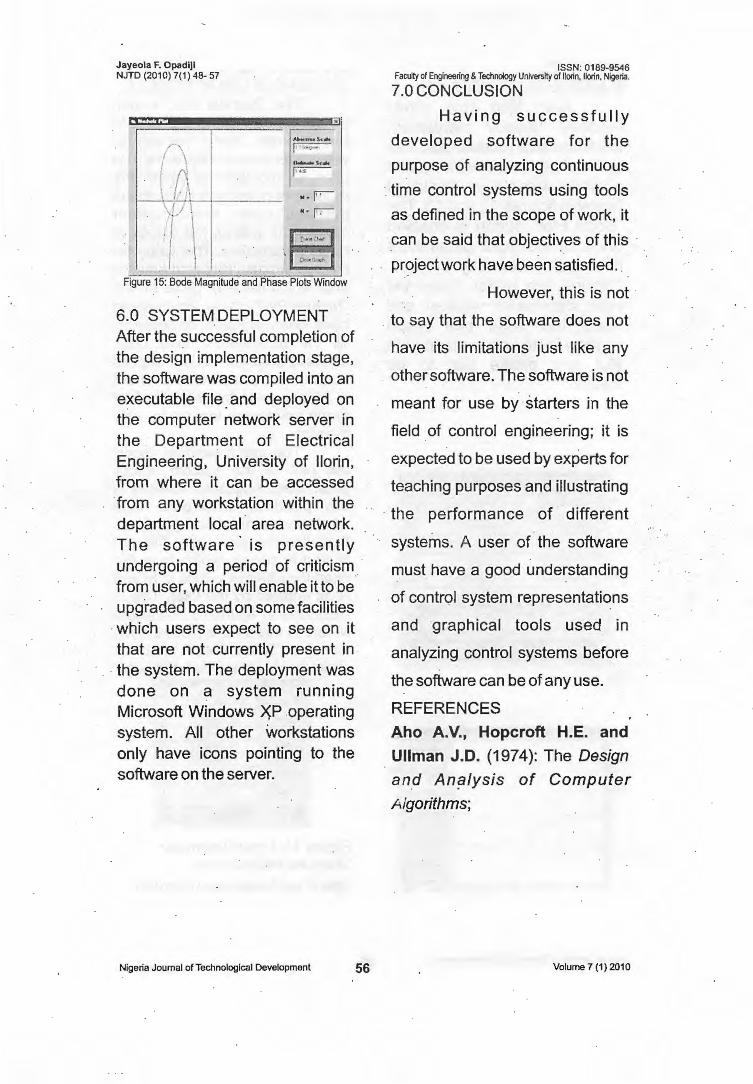
The graph window shows the plot of the system whose parameters had been entered in the prev_ious interface. This window also has two input fields that allow the user to plot different M and N circles, which form the chart for different values of M and N as entered by the user. This is illustrated in figure 15. Individual M and N circles are plotted each time the "Trace Chart'' button is clicked with a new value of M or N.

H[tiJ r p.e10 o 1· wl ....... ,.._..._ ............. l'"3 .._ .:- Ji"-;:J

' '"z.,' P-S-... r­,..._ r-,...,z... r­f#>Z... r-

Figure 14: Input Parameter Sheet for Nichols Plot Figure 14: Input Parameter Sheet for Nichols Plot

Volume 7 (1) 2010.

Jayeola F. Opad lJI NJTD (2010) 7(1) 48- 57

T\ Figure 15: Bode Magnitude and Phase Plots Window

6.0 SYSTEM DEPLOYMENT After the successful completion of the design implementation stage, the software was compiled into an executable file. and deployed on the computer network server in the Department of Electrical Engineerin·g, University of llorin, from where it can be accessed ·from any workstation within the department local · area network. The software· is presen tly undergoing a period of criticism from user, which will enable it to be upg'raded based on some facilities which users expect to see on it that are not currently present in the system. The deployment was done on a system running Microsoft Windows XP .operating system. All other workstations only have icons pointing to the software on the server.

Nigeria Journal of Technological Development 56

ISSN: 0189-9546 Faculty of Engineering & Technology University of llorin, llorin. Nigeria.

7.0 CONCLUSION

Having successfully

developed software for the

purpose of analyzing continuous

time control systems using tools

as defined in the scope of work, it

can be said that objectives of this

project work have been satisfied.

However, this is not

to say that the software does not

have its limitations just like any

other software. The software is not

meant for use by starters in the

field of control engineering; it is

expected to be used by experts for

teaching purposes and illustrating

the performance of different

systems. A user of the software

must have a good understanding

of control system representations

and graphical tools used in

analyzing control systems before

the software can be of any use.

REFERENCES

Aho A.V., Hopcroft H.E. and Ullman J.D. (1974): The Design

and Analysis of Computer

Algorithms;

Volume 7 (1) 2010

Jayeola F. Opadijl NJTO (2010) 7(1)48- 57

Addison-Wesley Publishing Company, Essex, England.

Aptech Limited ( 1999): Programming Skills and the Internet (First Edition), Aptech, India.

· Brassard G. · and Bratley P .. (1996): Fundamentals of Algorithms; ·Prentice Hal(, New Jersey, USA.

Nwadiani M. and Apotu N.E. (2002): Academic Staff Turnover in Nigerian Universities; Education, Vol.123.

Oni B~ (1999): The Nigerian University Today and the

· Challenges of the Twenty-first Century; Monograph, No. 60. Institute for World Economics and .International Management, University of Bremen, Bremen, . Germany.

Nigeria Joumal of Technological Development 57

ISSN: 0189-9546 Faculty of Engineering & Technology University of llOfin, Dorin, Nigeria.

Volume 7 (1) 2010