Embed Size (px)
Citation preview
University of IowaIowa Research Online
Theses and Dissertations
Summer 2009
Eye tracking metrics for workload estimation inflight deck operationsKyle Kent Edward EllisUniversity of Iowa
Copyright 2009 Kyle Kent Edward Ellis
This thesis is available at Iowa Research Online: https://ir.uiowa.edu/etd/288
Follow this and additional works at: https://ir.uiowa.edu/etd
Part of the Industrial Engineering Commons
Recommended CitationEllis, Kyle Kent Edward. "Eye tracking metrics for workload estimation in flight deck operations." MS (Master of Science) thesis,University of Iowa, 2009.https://ir.uiowa.edu/etd/288.

EYE TRACKING METRICS FOR WORKLOAD ESTIMATION
IN FLIGHT DECK OPERATIONS
by
Kyle Kent Edward Ellis
A thesis submitted in partial fulfillment of the requirements for the Master of Science degree
in Industrial Engineering in the Graduate College of The University of Iowa
July 2009
Thesis Supervisor: Associate Professor Thomas Schnell

Copyright by
KYLE KENT EDWARD ELLIS
2009
All Rights Reserved
Graduate College
The University of Iowa Iowa City, Iowa
CERTIFICATE OF APPROVAL
_______________________
MASTER’S THESIS
_______________
This is to certify that the Master’s thesis of
Kyle Kent Edward Ellis
has been approved by the Examining Committee for the thesis requirement for the Master of Science degree in Industrial Engineering at the July 2009 graduation.
Thesis Committee: _______________________________
Thomas Schnell, Thesis Supervisor
_______________________________
Andrew Kusiak
_______________________________
Yong Chen
_______________________________
Kara Latorella

ACKNOWLEDGMENTS
Completion of this study and thesis would not have been possible without the
collaboration, assistance, and support of many, many individuals at the Operator
Performance Laboratory, NASA, Smarteye Inc, and the University of Iowa. I would
specifically like to thank Tom Schnell for overseeing and advising the project with
expertise in aviation design of experiment and technical background; Kara Latorella and
associates at NASA for funding the Operator State Classification Project; Dan Burdette
for his comprehensive review of eye tracking in flight deck operations; Michael Keller
for his seemingly unlimited talent in software engineering capable of encompassing the
endless list of changes and random incorporations this study demanded; Jon Plumpton for
his assistance in data analysis and hardware repair; Mathew Cover for his assistance in
keeping the computer hardware components up and running in times of crisis, as well as
his expertise in advising me from the perspective of a fellow graduate student; Magnus
Sjölin of Smarteye for his assistance with optimizing the eye tracking system in OPL’s
737 simulator; Carl Richey for his immediate assistance whenever necessary to repair the
simulator during times of mechanical failure; Ron Daiker for his assistance with flight
test engineering; Chris Stadler for many hours of tireless effort spent in manual data
analysis and pre-processing, just as many hours spent collecting data as a flight test
engineer, and developing a foolproof startup guide to effectively run the simulator for
future studies to come.
iii
TABLE OF CONTENTS
LIST OF TABLES .............................................................................................................. v
LIST OF FIGURES ........................................................................................................... vi
LIST OF EQUATIONS ..................................................................................................... ix
CHAPTER 1. INTRODUCTION ...................................................................................... 1
Statement of the Problem ........................................................................................ 1
Proposed Solution Approach .................................................................................. 1
Contributions........................................................................................................... 2
Practical contribution .................................................................................. 2
Theoretical contributions ............................................................................ 2
CHAPTER 2. BACKGROUND ........................................................................................ 4
Review of Technical Literature .............................................................................. 4
Mechanism of visual search ........................................................................ 4
Impact of individual differences ................................................................. 6
Experience-related differences .................................................................... 6
Physical-related differences ........................................................................ 7
Environment-related differences ................................................................. 8
Existing eye tracking metrics, trends and measures ................................... 9
Analysis and ranking of existing eye tracking metrics ............................. 23
CHAPTER 3. 737-800 FLIGHT DECK EYE TRACKING RESEARCH STUDY ....... 25
Methodology ......................................................................................................... 25
Hypothesis................................................................................................. 25
Apparatus .................................................................................................. 25
Smarteye Eye Tracking System ................................................................ 31
Design of Experiment ............................................................................... 33
Participants ................................................................................................ 44
Independent Variables .............................................................................. 45
Dependent Variables ................................................................................. 46
Flight Test Matrix ..................................................................................... 49
Flight Test Results ................................................................................................ 50
Visual scanning ......................................................................................... 50
Flight performance .................................................................................... 50
Flight Test Conclusions ........................................................................................ 51
CHAPTER 4. DATA ANALYSIS AND ALGORITHM DEVELOPMENT ................. 52

iv
Data Set ................................................................................................................. 52
Analysis Methodology .......................................................................................... 60
Results Conclusion................................................................................................ 70
CHAPTER 5. CATS INTEGRATION ............................................................................ 71
Cognitive Avionics Tool-Set (CATS) .................................................................. 71
Algorithm Implementation.................................................................................... 76
Real-Time Workload Estimation .............................................................. 77
Utility of Algorithm for Real-Time Classification ................................... 77
Industry Utilization of Operator State Classification Information ....................... 78
CHAPTER 6. FUTURE RESEARCH ............................................................................. 79
Further Initiatives to Be Pursued .......................................................................... 79
APPENDIX ................................................................................................................... 81
BIBLIOGRAPHY ........................................................................................................... 101

v
LIST OF TABLES Table 1. Collected Eye Tracking Metrics 24
Table 2. Subjective Responses 48
Table 3. Eye Tracking Metric List 49
Table 4. Reduced Sample Flight Test Matrix 49
Table 5. IOS Collection Data 54
vi
LIST OF FIGURES Figure 1. Anatomy of the Human Eye ................................................................................ 5
Figure 2. Example of Fixation Map on Standard 737 EFIS PFD .................................... 20
Figure 3. Example of Fixation Map on Standard 737 EFIS PFD 2 ................................ 20
Figure 4. OPL 737-800 Flight Deck ................................................................................ 26
Figure 5. PFD EFIS........................................................................................................... 27
Figure 6. MFD NAV Display ........................................................................................... 28
Figure 7. 737-800 EICAS ............................................................................................... 29
Figure 8. 737 MCP Configuration .................................................................................... 30
Figure 9. 737 Smarteye Camera and Flasher Setup .......................................................... 33
Figure 10. KORD 9R Approach Flight Plan ..................................................................... 34
Figure 11. Pilot Approach and Landing Checklist ........................................................... 35
Figure 12. KORD ILS RWY 9R Approach Plate ............................................................. 36
Figure 13. Landing Visual Conditions at Decision Height .............................................. 38
Figure 14. Go-Around Visual Condition at Decision Height .......................................... 38
Figure 15. Bedford Workload Scale ................................................................................. 41
Figure 16. SART Assessment Card .................................................................................. 43
Figure 17. NASA-TLX Assessment Card ........................................................................ 44
Figure 18. Boxplot of Average Bedford Score vs. Land/Go-Around, Condition ............. 55
Figure 19. Average Bedford Workload Score Statistics ................................................... 56
Figure 20. Boxplot of SART Score vs. Land/Go-Around, Condition .............................. 56
Figure 21. SART Score Statistics ..................................................................................... 57
Figure 22. Boxplot of NASA-TLX Score vs. Land/Go-Around, Condition .................... 57
vii
Figure 23. NASA-TLX Total Statistics ............................................................................ 58
Figure 24. Average Bedford vs. SART Score Regression ................................................ 59
Figure 25. Average Bedford vs. NASA-TLX Total Regression ....................................... 59
Figure 26. Example Boxplot of ET Metric vs. Workload (Max HDG Fixation Duration vs. Workload) ............................................................................................................ 62
Figure 27. Eye Tracking Metric vs. Workload Repeated Measures ANOVA ................. 63
Figure 28. Eye Tracking Metrics vs. Workload Regression Model ................................ 64
Figure 29. Task vs. Workload Repeated Measures ANOVA ........................................... 66
Figure 30. Task + ET Metrics vs. Workload Repeated Measures ANOVA ..................... 67
Figure 31. Task + ET Metrics vs. Workload Regression .................................................. 69
Figure 32. CATS File Selection Window ......................................................................... 72
Figure 33. CATS Data Integrity Window ......................................................................... 73
Figure 34. CATS Data Query Window............................................................................. 74
Figure 35. CATS World Viewer Window ........................................................................ 75
Figure 36. CATS Eye Tracking Histogram Window........................................................ 76
Figure A1. Mean Fixation Duration vs. Workload Boxplot ............................................. 81
Figure A2. Global Fixation Frequency vs. Workload Boxplot ......................................... 82
Figure A3. Mean Saccade Length vs. Workload Boxplot ................................................ 82
Figure A4. Max Saccade Length vs. Workload Boxplot .................................................. 83
Figure A5. Mean Airspeed Fixation Duration vs. Workload Boxplot .............................. 83
Figure A6. Max Airspeed Fixation Duration vs. Worklaod Boxplot ............................... 84
Figure A7. Airspeed Fixation Frequency vs. Workload Boxplot ..................................... 84
Figure A8. Mean Altitude Fixation Duration vs. Workload Boxplot ............................... 85
Figure A9. Max Altitude Fixation Duration vs. Workload Boxplot ................................. 85
Figure A10. Altitude Fixation Frequency vs. Workload Boxplot .................................... 86
Figure A11. Mean Heading Fixation Duration vs. Workload Boxplot............................. 86

viii
Figure A12. Heading Fixation Frequency vs. Workload Boxplot .................................... 87
Figure A13. Mean OTW Fixation Duration vs. Workload Boxplot ................................. 87
Figure A14. Max OTW Fixation Duration vs. Workload Boxplot ................................... 88
Figure A15. Mean MCP Fixation Duration vs. Workload Boxplot .................................. 88
Figure A16. Max MCP Fixation Duration vs. Workload Boxplot ................................... 89
Figure A17. MCP Fixation Frequency vs. Workload Boxplot ......................................... 89
Figure A18. Mean MFD Fixation Duration vs. Workload Boxplot ................................. 90
Figure A19. Max MFD Fixation Duration vs. Workload Boxplot ................................... 90
Figure A20. MFD Fixation Frequency vs. Workload Boxplot ......................................... 91
Figure A21. Mean Y StdDev vs. Workload Boxplot ........................................................ 91
Figure A22. Mean X StdDev vs Workload Boxplot ......................................................... 92
Figure A23. NASA-TLX vs. Bedford Regression ............................................................ 92
Figure A24. SART vs. Bedford Regression...................................................................... 93
Figure A25. Global Composite Metric Repeated Measures ANOVA ............................. 94
Figure A26. ET Metric vs. Workload Regression ............................................................ 95
Figure A27. ET Metrics vs. Workload Repeated Measures ANOVA .............................. 96
Figure A28. Task + ET Metrics vs. Workload Regression ............................................... 97
Figure A29. Task + ET Metrics vs. Workload Repeated Measures ANOVA .................. 98
Figure A30. Task (including land decision) vs. Workload ANOVA ............................... 99
Figure A31. Task (incl. land decision) vs. Workload Repeated Measures ANOVA ..... 100
ix
LIST OF EQUATIONS
Equation 1. Entropy Equation .......................................................................................... 15
Equation 2. Relative Entropy Equation ............................................................................ 16
Equation 3: Scan-path indexing function .......................................................................... 22
Equation 4. SART Situational Awareness (SA) Equation ................................................ 42

x

1
CHAPTER 1.
INTRODUCTION
Statement of the Problem
For over a century, eye tracking has helped experimenters determine what an
individual views, providing clues to what the subject could be cognitively engaged in.
However, questions remain as to what metrics work best in determining subject state and,
more specifically, subject workload.
Proposed Solution Approach
The basic metrics within eye tracking, such as saccadic movement, fixations and
link analysis provide clear measurable elements that experimenters could use to create a
quantitative algorithm that reliably classifies operator workload.
Because eye tracking allows for non-invasive analysis of pilot eye movements,
from which a set of metrics can be derived to effectively and reliably characterize
workload, this research will generate quantitative algorithms to classify pilot state
through eye tracking metrics. Through the use of various eye tracking metrics and
measures, a correlation between these components will be regressed against pre-
determined workload levels as well as self-reported subjective workload ratings in
varying flight deck test scenarios. This will improve existing knowledge of eye tracking
in flight deck operations and will provide further advancement in the quest for operator
state classification.
2
Contributions
Practical contribution
Operators in today’s aircraft flight decks find themselves in various situations that
change their cognitive workload. Research to improve the interaction between the
operator and the aircraft interface will benefit by being able to analyze operator state
quantitatively as opposed to the historical standard of subjective feedback. This
eliminates the subjective bias across subjects and standardizes feedback to provide more
accurate analysis of operator state in different testing scenarios in flight deck operations.
This research is somewhat flight deck specific due to some of the eye tracking measures
being specific to flight deck operations, such as entropy, which is dependent on flight
task. However, some of the eye tracking metrics that are used to determine workload are
common across interfaces, such as fixation duration and blink rate.
Theoretical contributions
Current avionics are not aware of pilot real-time capabilities and limitations
resulting from varying workload levels. There exists the potential in various phases of
flight and circumstances for information overload in flight deck operations. Several
systems within the flight deck itself, such as the flight management system and tethered
autopilot, are very effective at making easy procedures easier and hard operations harder
in such circumstances; such is the case when unexpected occurrences happen in flight.
When the avionics being unaware of pilot state, it is impossible for the avionics to
provide dynamic displays that provide the proper information in the proper context and
3
with appropriate levels of automation for various situations based upon the pilot’s current
abilities.
The concept of the intelligent flight deck is currently being pursued by the
National Aeronautics and Space Administration (NASA), with specific interest in
characterizing operator state in flight deck operations. The goal is to use operator
workload and overall cognitive state effectively to optimize the flight deck interface.
Eye tracking as a remote unattached sensor providing a non intrusive solution that
is fully deployable in future flight decks with minor changes to current setup. NASA’s
IIFD objective to characterize operator state will be supported by these eye movement
behavior based workload algorithms.
4
CHAPTER 2.
BACKGROUND
Review of Technical Literature
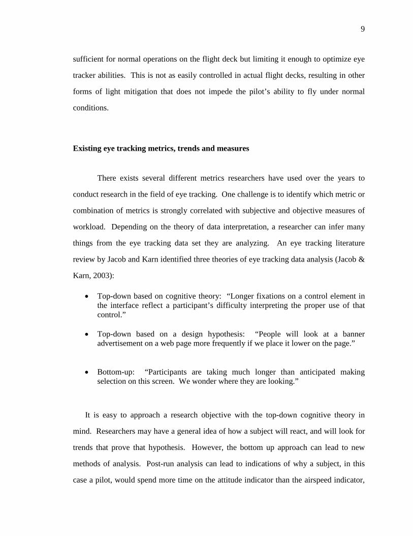
Mechanism of visual search
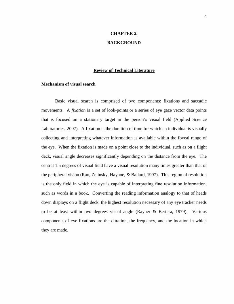
Basic visual search is comprised of two components: fixations and saccadic
movements. A fixation is a set of look-points or a series of eye gaze vector data points
that is focused on a stationary target in the person’s visual field (Applied Science
Laboratories, 2007). A fixation is the duration of time for which an individual is visually
collecting and interpreting whatever information is available within the foveal range of
the eye. When the fixation is made on a point close to the individual, such as on a flight
deck, visual angle decreases significantly depending on the distance from the eye. The
central 1.5 degrees of visual field have a visual resolution many times greater than that of
the peripheral vision (Rao, Zelinsky, Hayhoe, & Ballard, 1997). This region of resolution
is the only field in which the eye is capable of interpreting fine resolution information,
such as words in a book. Converting the reading information analogy to that of heads
down displays on a flight deck, the highest resolution necessary of any eye tracker needs
to be at least within two degrees visual angle (Rayner & Bertera, 1979). Various
components of eye fixations are the duration, the frequency, and the location in which
they are made.
5
Figure 1. Anatomy of the Human Eye
The eye movement from one fixation to the next is called a saccade. A saccade
connects one fixation to the next, and can be measured in terms of radial degrees.
Different components to a saccade include the length of the saccade (visual angle), the
speed of the saccade in degrees per second, and the direction of the saccade. When
reading, the eye makes rapid movements, as many as four to five per second, moving
from one fixation to the next, focusing on a few words each time (Rayner & Bertera,
1979). The eye does not transmit visual signals to the brain when making a saccade.
Therefore, a saccade is made each time information is obtained from one fixation and
another fixation is necessary to observe further information elsewhere.
Combining saccadic movements and their associated fixations a scan pattern or
scan path emerges. Since fixations only cover a finite space filled with information,
saccadic movements trace the area of desired information so fixations can collect all the
information necessary for the brain to interpret the overall image. Previous research
provides two suggestions connecting saccadic movements and fixations, concluding on
the meaning of scan paths: one proposal indicates that saccadic movements’ resulting
fixations allow for the formation of visual-motor memory to encode objects and scenes
6
(Noton & Stark, 1971). Another proposal originating from work done by Yarbus
suggests that changes in fixations are most commonly associated with the dynamic
demands of a given task (Yarbus, 1967).
Impact of individual differences
There are several components to the differences in eye tracking performance and
movement behavior observed across individual subjects: Experience of the subject in
performing the given task, physical differences (e.g. Blue versus brown eyes), and
environmental condition differences (e.g. vibration). Experience related differences
cannot be changed without future manipulation of the pilots themselves through
increased training and experience. The easiest target to minimize individual changes is
the physical-related differences by simply screening subjects to fit the optimal
specifications that work well with the eye tracker.
Experience-related differences
The quality of the eye tracking itself is not affected by differences among pilots’
experience, however, the eye tracking metrics themselves can be drastically different.
Past research has demonstrated the difference between novice and more experienced
participants in various usability studies (Fitts, Jones, & Milton, 1950); (Crosby &
Peterson, 1991); (Card, 1984); (Altonen, Hyrskykari, & Raiha, 1998). Common effects
are observed in fixation durations, number of fixations, saccadic movements, and scan
pattern changes. Experienced pilots will typically be more comfortable while performing
a flight task with a basic knowledge of what they need to look at to obtain the

7
information they need. This increases the efficiency of their eye behavior, resulting in a
difference in eye tracking metrics in contrast to a novice pilot.
Physical-related differences
Subject’s eyes are of paramount concern due to the variance in quality of eye
tracking data that can be obtained due to physical differences in the eyes themselves.
Subjects with a history of ocular trauma, various ophthalmological diseases (previous or
current), lazy eyes, pathologic nystagmus or other ocular disorders, and different forms of
corrective lenses including both eyeglasses and contact lenses are likely to cause issues
for researchers attempting to obtain consistently high quality eye tracking data. Because
of this, it is highly recommended that researchers screen their subjects prior to
participation in any eye tracking study to ease the effort required to collect quality eye
tracking data from their eye tracker.
Pupil color greatly impacts the quality of eye tracking for many eye trackers.
High precision eye trackers require a sharp contrast between the pupil and the iris. Bright
pupil systems require direct infrared reflection off of the retina therefore, subjects with
blue eyes are often times easier to track. This is due to blue eyes containing less IR-
reflective melanin in the iris. In contrast to this, brown or hazel eyes are usually ideal for
eye tracking systems that utilize a dark pupil contrast. (Boyce, Ross, Monaco, Hornak, &
Xin, 2006); (Wang, Lin, Liu, & Kang, 2005).
Pilots who may be sleep deprived also pose another form of problem. Eyelid
closure can become an issue when the eyelid itself begins to cover portions of the pupil.
Many remote eye trackers can operate with some part of the pupil being covered, but a
majority must still be shown in order for the processing algorithms to calculate the
circular center of the pupil that is used as an integral part of gaze vector calculation.
8
Corrective lenses, such as glasses, pose reflection issues that pose as the biggest
threat to eye tracking quality. Lenses posing the largest problem are lenses with hard-
edged bi- or tri-focal lenses due to distortion of the eye image as seen from the
perspective of the eye tracking cameras. Distortions typically occur due to lens shape,
causing problems with systems using corneal reflection, bright retinal reflection, dark
pupil circle, limbus or iris features, etc. Soft contact lenses typically do not cause
problems however, hard contacts can cause edge problems in bright pupil systems
typically caused by dirt or dust trapped beneath the lens. Typically single vision
corrective eye glasses do not cause problems unless they have an anti-reflective coating.
Lenses with curved front surfaces will often times because of problems caused by
reflecting the infrared source back into the camera.
Environment-related differences
There exist several environmental factors that can become problematic to the
testing environment incorporating an eye tracker. Many of these issues are observed in
dynamic location flight decks, such as that of an actual aircraft flight deck that would
experience varying light conditions, turbulence, and other vibration effects that move the
pilot’ head relative to the eye tracking camera. Since the system is based upon visual
contrast, extreme light behaviors pose the greatest threat; usually the only problem in
fixed base simulators such as OPL’s 737-800 simulator.
Problems associated with extreme ambient light include; too small of pupil
diameter, squinting that places the eyelid over the pupil, glare that causes the pilot to
change their eye tracking behavior, and degradation of the eye tracker ability to detect
features of the face for head tracking purposes. Thankfully, in most simulators the
ambient light levels are easily controllable, making it simple to adjust light to be
9
sufficient for normal operations on the flight deck but limiting it enough to optimize eye
tracker abilities. This is not as easily controlled in actual flight decks, resulting in other
forms of light mitigation that does not impede the pilot’s ability to fly under normal
conditions.
Existing eye tracking metrics, trends and measures
There exists several different metrics researchers have used over the years to
conduct research in the field of eye tracking. One challenge is to identify which metric or
combination of metrics is strongly correlated with subjective and objective measures of
workload. Depending on the theory of data interpretation, a researcher can infer many
things from the eye tracking data set they are analyzing. An eye tracking literature
review by Jacob and Karn identified three theories of eye tracking data analysis (Jacob &
Karn, 2003):
• Top-down based on cognitive theory: “Longer fixations on a control element in the interface reflect a participant’s difficulty interpreting the proper use of that control.”
• Top-down based on a design hypothesis: “People will look at a banner advertisement on a web page more frequently if we place it lower on the page.”
• Bottom-up: “Participants are taking much longer than anticipated making selection on this screen. We wonder where they are looking.”
It is easy to approach a research objective with the top-down cognitive theory in
mind. Researchers may have a general idea of how a subject will react, and will look for
trends that prove that hypothesis. However, the bottom up approach can lead to new
methods of analysis. Post-run analysis can lead to indications of why a subject, in this
case a pilot, would spend more time on the attitude indicator than the airspeed indicator,

10
both of which are of high importance. The answers to such questions can lead to further
understanding of pilot workload, and what is consuming their cognitive capacity and
why.
Initial research in literature review will follow a top-down cognitive theory
approach to identifying eye tracking metrics from a simple view of quantifying the raw
data collected during this study. Understanding how the research team is attempting to
interpret the data is important in determining not only what metrics to use but also how
they will be used.
NASA Langley Flight Research has conducted several eye tracking studies in the past
resulting in a basic starting platform to compile metrics for many future research
initiatives. From this research, a series of basic definitions is utilized to quantify various
sets of eye tracking data:
• Average Dwell Time – The total time spent looking at an instrument divided
by the total number of individual dwells on that instrument.
• Dwell percentage – Dwell time on a particular instrument as a percent of total
scanning time.
• Dwell Time – The time spent looking within the boundary of an instrument.
• Fixation – A series of continuous lookpoints which stay within a pre-defined
radius of visual degrees.
• Fixations per dwell – The number of individual fixations during an instrument
dwell.
• Glance – A “subconscious” (i.e., non-recallable) verification of information
with a duration histogram peaking at 0.1 seconds. (also referred to as an
“orphan”)
• Lookpoint – The current coordinates of where the pilot is looking, frequency
of data points depending on the eye tracking system used.
• One-way transition – The sum of all transitions from one instrument to
another (one direction only) in a specified instrument pair.
11
• Out of track – A state in which the eye tracking system cannot determine
where the pilot is looking, such as during a blink or when the subject’s head
movement has exceeded the tracking capabilities of the system setup.
• Saccade – The movements of the eye from one fixation to the next. Also
considered to be the spatial change in fixations.
• Scan – Eye movement technique used to accomplish a given task. Measures
used to quantify a scan include (but are not limited to) transitions, dwell
percentages, and average dwell times.
• Transition – The change of a dwell from one instrument to another.
• Transition rate – The number of transitions per second.
• Two-way transition – The sum of all transitions between an instrument pair,
regardless of direction of the transition.
(Harris, Glover, & Spady, 1986)
Area of Interest
Areas of interest are regions specified over a field of view that hold significant
meaning or indicate a specific source of information. The definition of areas of interest is
at the discretion of the researcher. It is critically important to specify what that area of
interest represents in order to compile meaningful results. Areas of interest are very task
specific, depending on what form of visual scan will be required to complete the task, and
what interface is being used (Jacob & Karn, 2003). In flight, regions of interest often
include the heads down displays, often broken down into smaller regions including the
airspeed indicator, altimeter, attitude indicator, heading indicator, etc.
The limiting factors to the area of interest definition rest solely on the capabilities
of the eye tracking system being used. An area of interest can only be as small as the eye
tracking system has consistently high performance accuracy of eye gaze vectors. The
smaller a region of interest, the more accurate a system must be to identify a person’s eye
12
gaze within that region. An area of interest must be specific enough to include the
important details of a test platform’s field of view, but must not be so specific that no
meaningful data is attainable due to the noise of eye tracker inaccuracy.
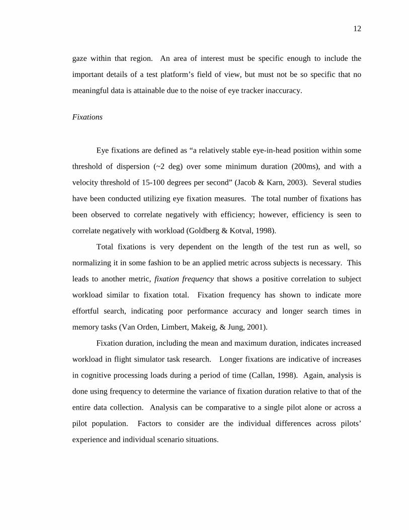
Fixations
Eye fixations are defined as “a relatively stable eye-in-head position within some
threshold of dispersion (~2 deg) over some minimum duration (200ms), and with a
velocity threshold of 15-100 degrees per second” (Jacob & Karn, 2003). Several studies
have been conducted utilizing eye fixation measures. The total number of fixations has
been observed to correlate negatively with efficiency; however, efficiency is seen to
correlate negatively with workload (Goldberg & Kotval, 1998).
Total fixations is very dependent on the length of the test run as well, so
normalizing it in some fashion to be an applied metric across subjects is necessary. This
leads to another metric, fixation frequency that shows a positive correlation to subject
workload similar to fixation total. Fixation frequency has shown to indicate more
effortful search, indicating poor performance accuracy and longer search times in
memory tasks (Van Orden, Limbert, Makeig, & Jung, 2001).
Fixation duration, including the mean and maximum duration, indicates increased
workload in flight simulator task research. Longer fixations are indicative of increases
in cognitive processing loads during a period of time (Callan, 1998). Again, analysis is
done using frequency to determine the variance of fixation duration relative to that of the
entire data collection. Analysis can be comparative to a single pilot alone or across a
pilot population. Factors to consider are the individual differences across pilots’
experience and individual scenario situations.

13
Gaze
Very similar to the fixation metric, gaze analyzes the grouping of fixations within
a single region of interest. Much of Fitts’ research focused on analysis of the gaze
metric, including gaze rate (# of gazes / minute) on each area of interest, gaze duration
mean and gaze percentage (proportion of time) in each area of interest for 40 pilots flying
an aircraft landing approach (Fitts, Jones, & Milton, 1950). Gaze metrics focus more on
the area of interest and what it represents, not only the measure of a fixation in any given
region of space.
The gaze metric places meaning behind the location of where a fixation occurs,
with the region for which a gaze is calculated can be of any size depending on the area of
interest. Measures within the gaze metric include the number of fixations within a single
gaze, the total number of gazes, the frequency of gaze and the duration of gaze, including
the mean and maximum statistics of this single measure (Hendrickson, 1989).
Saccadic Movement
Measures of saccadic movement are often times neglected in usability research
initiatives because many of its close relation to fixations measures, which are easier to
examine are used instead. There are several metrics available within the realm of
saccadic eye movements that are unique and potentially useful in studies involving task
oriented research. The length of the saccade, as well as the speed of which the saccade is
made are both very easily calculated measures, simply calculating the distance from one
fixation to the next in an ordered pair.
The frequency of longer length saccadic movements could indicate a correlation
of decreased efficiency, and potentially an increase in perceived workload. The
14
frequency of specific length saccadic movements requires a limit be set to determine
what a longer length saccadic movement is. This is dependent upon the specified areas of
interest. Usability research has used the ratio of fixation to saccade times as a measure
for analysis (Kotval & Goldberg, 1998). Another method in which to analyze saccadic
movement is to simply correlate the average saccadic movement distance over a period of
time and track the changes throughout a test run. Further research must be done to
validate the inferences associated with the subsets of saccadic movement metrics.
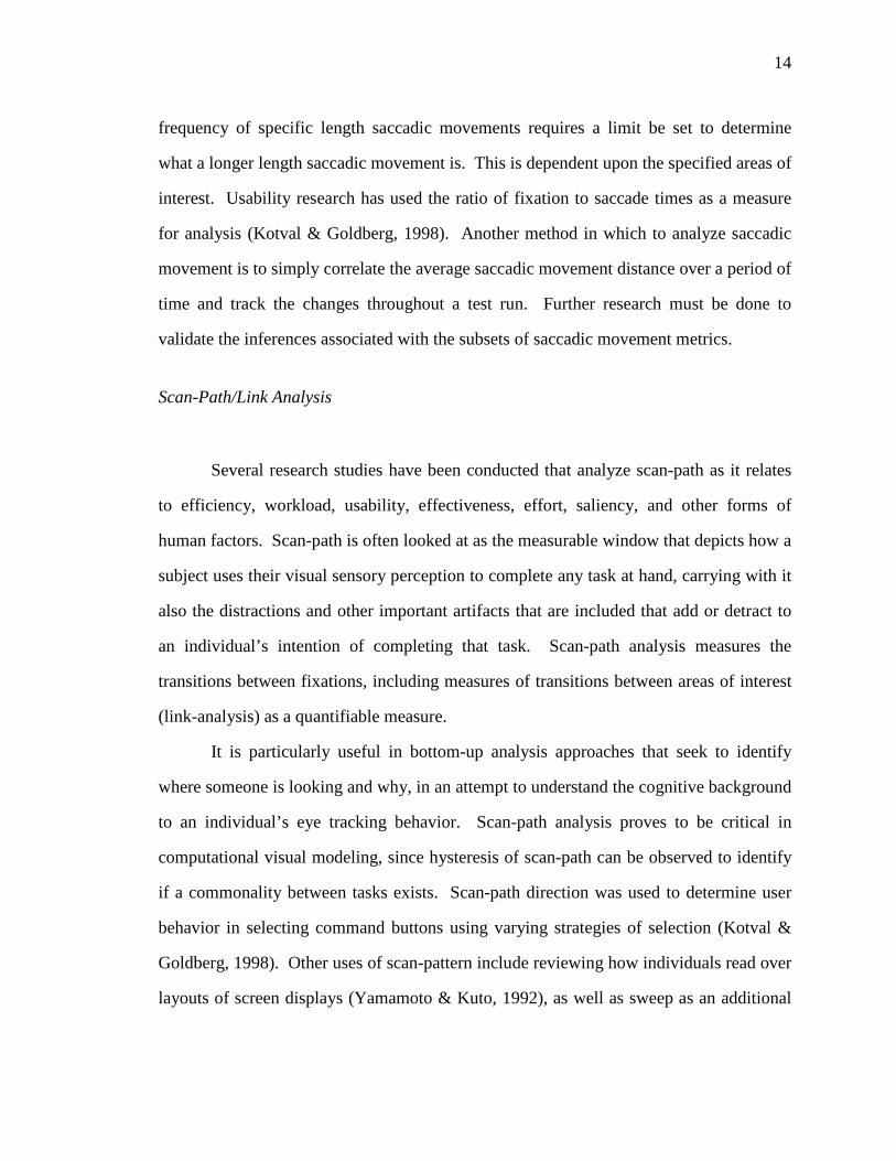
Scan-Path/Link Analysis
Several research studies have been conducted that analyze scan-path as it relates
to efficiency, workload, usability, effectiveness, effort, saliency, and other forms of
human factors. Scan-path is often looked at as the measurable window that depicts how a
subject uses their visual sensory perception to complete any task at hand, carrying with it
also the distractions and other important artifacts that are included that add or detract to
an individual’s intention of completing that task. Scan-path analysis measures the
transitions between fixations, including measures of transitions between areas of interest
(link-analysis) as a quantifiable measure.
It is particularly useful in bottom-up analysis approaches that seek to identify
where someone is looking and why, in an attempt to understand the cognitive background
to an individual’s eye tracking behavior. Scan-path analysis proves to be critical in
computational visual modeling, since hysteresis of scan-path can be observed to identify
if a commonality between tasks exists. Scan-path direction was used to determine user
behavior in selecting command buttons using varying strategies of selection (Kotval &
Goldberg, 1998). Other uses of scan-pattern include reviewing how individuals read over
layouts of screen displays (Yamamoto & Kuto, 1992), as well as sweep as an additional
15
scan-path metric indicating a progressive trend in scan-path direction (Altonen,
Hyrskykari, & Raiha, 1998).
From a top-down approach scan-path is seemingly less useful. Issues with real
time analysis of scan-path as its own metric are that it is difficult to quantify since it is a
combination of saccadic movements and fixations in a seemingly random sequence. A
scan-path can be used to describe the behavior of an individual’s gaze in several areas of
interest over time, but only once the scan-path has been made, making it a post process
analytical method. Attempts to quantify scan-path have been made by indexing spatial
randomness of scan-path behavior relative to what is expected for the given task (Di
Nocera, Terenzi, & Camilli, 2006) (see below, Scan-Path Contrast Indexing).
Visual Entropy
Other metrics utilizing the idea of scan-paths have been developed by researchers
to indicate when a subject’s observed scan-path pattern changes. Entropy calculates the
change observed in an individual’s scanning behavior by calculating the standard
deviation of fixations (randomness) over a previous period of time and determining the
rate of change of that standard deviation in real time. Entropy can be observed by
viewing fixation densities over time, particularly useful when done using a fixation map
(see below). Entropy as a correlative metric is approach by inferring that as workload
increases the observed scan-path becomes less random (Di Nocera, Terenzi, & Camilli,
2006). To contrast this inference, research done by Hilburn suggests that a decrease in
mental workload should increase the randomness of the scan-path behavior (Hilburn,
2004).
)/1(log2 ii ppHEntropy ∑==
Equation 1. Entropy Equation

16
A recent car study utilizes entropy to correlate effectively with a driver’s
workload by using it as a prediction for where drivers will look depending on the task at
hand. By assuming when situations are in high entropy, or high levels of randomness, the
probability of looking at everything an equal number of times will transition between all
areas of interest and stimuli at near equal frequencies. Each area of interest or fixation
point is associated with a state-space probability of subject focus (pi). The state-space
probability changes over time as scan-path trends change, therefore, changing the entropy
value (H) (Gilland, 2008).
When focus begins to shift with specific intent due to an induced task or stimuli
the attention of the subject is directed to a narrower range of fixation points, thereby
decreasing the calculated entropy value. This occurs due to the frequency of other
possible fixations and transitions to other areas of interest decreases (lowering the pi
value of a given state-space) since a more systematic pattern of fixations emerges when
the subject is in a state of higher focus or higher workload (Gilland, 2008). Important for
the use of real-time calculation of entropy if used for workload correlation is Relative
Entropy. This calculates the entropy relative to the highest value observed for that
particular data set or test run.
max/_ HHENTROPYRELATIVE observed=
Equation 2. Relative Entropy Equation
In contrast to the research that provides evidence supporting a low workload –
high entropy (increased randomness) correlation, this may not as effectively correlate
17
with tasks on a flight deck. Pilots are heavily trained on proper eye scan techniques for
all phases of flight, specifically pilots maintaining an IFR pilot’s license. Pilots trained
on instrument flight are trained to look at particular instruments in a specific order to
ensure that the state of the aircraft is constantly monitored during all phases of flight.
With this training eye scan patterns will remain very ordered in constant flight conditions
with no change in pilot demands. It may be that eye scan will become more random
when demand is increased and a pilot is unable to pay enough attention to their trained
eye scan pattern. Entropy changes will still be associated with changes in flight task and
workload, but the correlation may not be the same as has been observed in previous
research.
Blink Rate
Blink rate has proven to be a metric that correlates with workload regardless of
the task variance. Research using air traffic controllers in high and low workload
situations suggests that increases in workload negatively correlate with blink rate
(Brookings, Wilson, & Swain, 1996); (Wilson, Purvis, Skelly, Fullenkamp, & Davis,
1987). The fundamental belief being that workload is higher requiring more focused
attention and a general increase in visual load. Blinks therefore occur less often so it is
less likely to miss critical information. This requires the amount of time the eye is
collecting information to be increased thereby resulting in a decreased blink rate
(Brookings, Wilson, & Swain, 1996).
As an active response to pilot workload correlations, blink rate relative to a
baseline average yields the same inverse relationship as shown in a research study done
visuospatial memory tasks (Van Orden, Limbert, Makeig, & Jung, 2001). Other research
indicates the time between blinks, called interblink interval, positively correlates with
workload (Brookings, Wilson, & Swain, 1996). This measure is simply a derivative of

18
the blink rate metric, calculating the time it takes to make a single blink. With an eye
tracker that can detect blink rates, blink rate as a metric for analysis proves to be a robust
option.
Pupilometry
Pupil changes in dilation and other pupilometry trends have been shown to be
instigated by changes in cognitive processing. Pupil diameter has been observed to
increase with increased cognitive loading in a color coding and symbolic tactical display
study (Backs & Walrath, 1992). Using baseline pupil diameter, the relative changes in
diameter were used to correlate with workload levels of subjects identifying several
symbols on various displays. Pupil dilation tends to be indicative of increased demand
for information processing.
There are two forms of pupil changes; dynamic, such as observed in cognitive
processing of discrete sentences (Just & Carpenter, 1993), or sustained pupil changes as
seen during digit span recalls (Granholm, Asarnow, Sarkin, & Dykes, 1996). Depending
on what type of workload tasks are, the appropriate form of pupillary response is
collected. In flight deck operations it is possible for both forms of pupillary responses to
be present, as pilots are required to both read information form heads down displays as
well as recall information from checklists and radio calls.
With information processing becoming the driver for changes in pupil metrics, it
is not task specific and can be applied as a general correlate to workload. The same
correlations are likely to apply across testing platforms (i.e. a flight deck or a computer
screen). One setback is the demand for high sample rate of pupilometry data from the
eye tracker. Due to the speed at which the pupil diameter changes, sample rates upwards
of 60 Hz is required to capture sufficient data capable of monitoring significant changes
pupil dilation (Just & Carpenter, 1993); (Granholm, Asarnow, Sarkin, & Dykes, 1996).
19
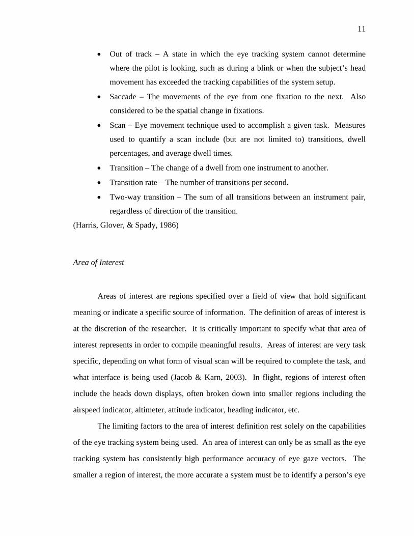
Fixation Maps
Fixation mapping is the “analysis of eye-movement traces” of a given scene. It is
often considered a more complex eye tracking measure as it requires more complex
analysis of multiple eye tracking metrics, such as mean fixation duration. A fixation map
is used in the quantification of the similarity of traces and the degree of coverage by the
fixations of a visual stimulus (Wooding, 2002). By mapping the fixations across a visual
scene, such as a flight deck, provides a 2-dimensional record of fixations over a specified
time, tfm. The timing variable can be changed to incorporate situation specific analysis or
to analyze the entire test run as a whole. It depends on the testing scenario as to how long
a fixation map retains its fixation history.
A fixation map is created by giving 2-dimensional coordinates to the fixation
itself, and then quantifying it by assigning pixel definition ‘d’ to that location. The
longer and more frequently a given location is fixated upon the greater the value d is.
Over time various d values will exist across the fixation map, providing a landscape that
describes the eye tracking fixation behavior over a given time tfm.
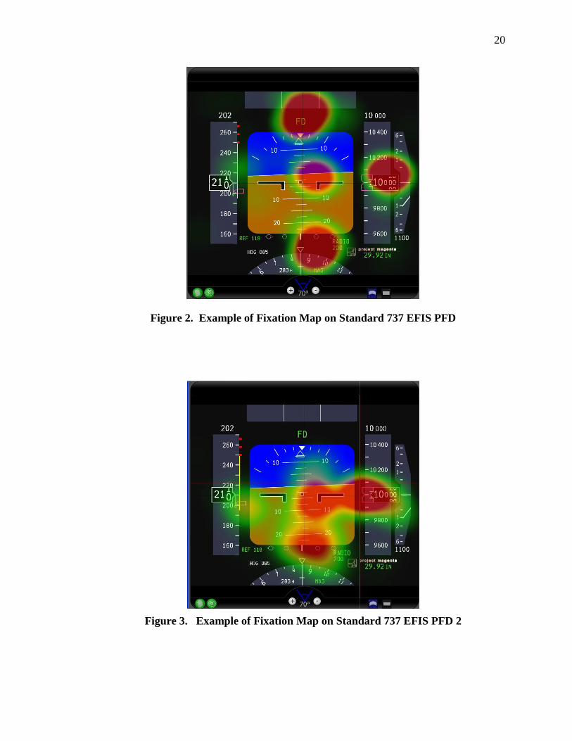
20
Figure 2. Example of Fixation Map on Standard 737 EFIS PFD
Figure 3. Example of Fixation Map on Standard 737 EFIS PFD 2

21
Depending on the type of analysis the fixation map ‘d’ values may be normalized
to make comparison across different fixation maps easier. To normalize the fixation
map, the greatest value of d is given a value of 1. For analysis to determine if a fixation
map contains a greater number of areas of interest (more fixation clusters), normalization
is not desirable. To determine areas of interest as specified by the eye tracking fixations
a value of dcrit may be assigned to a fixation map indicating where areas of interest exist.
This value can be shifted to eliminate/create more areas of interest depending on the
circumstances of analysis. By increasing dcrit there will be fewer areas of interest
specified, and in contrast by decreasing dcrit there will be more areas of interest.
Analysis to determine visual coverage is done by assigning dcrit and then assigning
a 1 to all d values greater than dcrit and a 0 to all d values less than dcrit. The sum of the
values of the new binary d values divided by the total number of existing d values (the
area of the map) provides the proportion of the map covered by fixations as prescribed by
the dcrit assignment (Wooding, 2002).
Fixation maps can be further analyzed comparatively by taking the differences of
d values and creating a new fixation map of differences. The remainder values indicate
where there is contrast between the two fixation maps, larger absolute values indicating
larger variance. This is done using normalized fixation maps only so relativity is
maintained between the fixation maps.
When analyzing fixation maps it is not the analysis of fixation order, but the
location of the fixation that is important. Another method to analyzing fixation maps are
done by using standard deviation of fixations from a determined mean location. This is
essentially determining the dispersion of fixations across a scene which is scene
dependent and not valid for varying flight deck interfaces.
22
Scan-Path Contrast Indexing
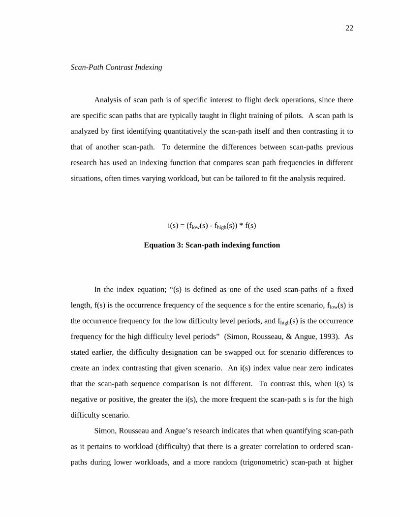
Analysis of scan path is of specific interest to flight deck operations, since there
are specific scan paths that are typically taught in flight training of pilots. A scan path is
analyzed by first identifying quantitatively the scan-path itself and then contrasting it to
that of another scan-path. To determine the differences between scan-paths previous
research has used an indexing function that compares scan path frequencies in different
situations, often times varying workload, but can be tailored to fit the analysis required.
i(s) = (flow(s) - fhigh(s)) * f(s)
Equation 3: Scan-path indexing function
In the index equation; “(s) is defined as one of the used scan-paths of a fixed
length, f(s) is the occurrence frequency of the sequence s for the entire scenario, flow(s) is
the occurrence frequency for the low difficulty level periods, and fhigh(s) is the occurrence
frequency for the high difficulty level periods” (Simon, Rousseau, & Angue, 1993). As
stated earlier, the difficulty designation can be swapped out for scenario differences to
create an index contrasting that given scenario. An i(s) index value near zero indicates
that the scan-path sequence comparison is not different. To contrast this, when i(s) is
negative or positive, the greater the i(s), the more frequent the scan-path s is for the high
difficulty scenario.
Simon, Rousseau and Angue’s research indicates that when quantifying scan-path
as it pertains to workload (difficulty) that there is a greater correlation to ordered scan-
paths during lower workloads, and a more random (trigonometric) scan-path at higher
23
workloads. Correlation in subject scan-path index regressed against workload varied
from 8% to 20%, which is still a notable for practical purposes of using the scan-path
measure. This indicates that workload can be determined from scan-path. However,
Simon, Rousseau and Angue argue that this analysis is tedious to perform and is notably
more difficult to do automatically as would be desirable.
Analysis and ranking of existing eye tracking metrics
There are several eye tracking metrics that can be chosen from previous research
to provide quantitative measures to analyze gaze vector data. The challenge exists in
determining what metrics are specific to eye tracking, are general metrics that correlate
with workload across tasks, and what metrics are simply of no use. The issue at hand is
that visual scanning requirements change frequently as a function of the flight maneuver
task (Hankins & Wilson, 1998); (Itoh, Hayashi, Tsukui, & Saito, 1990). Metrics must be
chosen either be task specific, or be applicable to all forms of workload scenarios. The
other limiting factor is the capabilities of the eye tracker itself. If the collection rate is not
fast enough some metrics will not be effective, such as pupilometry measures that require
upwards of 60 hertz sample rates.
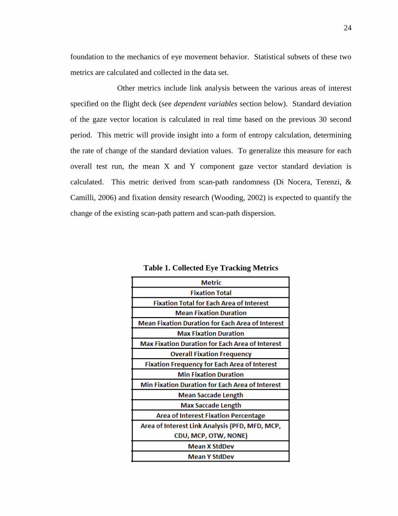
A compiled list of the core eye tracking metrics has been compiled that are to be
used for the research initiatives in estimating workload in flight deck operations.
Advanced eye tracking metrics such as entropy and fixation maps are calculated and
listed in the data analysis section of this report. Further definition of utilized metrics can
be found in the dependent variables section of chapter 3. These metrics were selected for
their ability to be utilized not only by themselves, but as composites to more advanced
metrics. Fixations and saccadic movements are core metrics due to their being the
24
foundation to the mechanics of eye movement behavior. Statistical subsets of these two
metrics are calculated and collected in the data set.
Other metrics include link analysis between the various areas of interest
specified on the flight deck (see dependent variables section below). Standard deviation
of the gaze vector location is calculated in real time based on the previous 30 second
period. This metric will provide insight into a form of entropy calculation, determining
the rate of change of the standard deviation values. To generalize this measure for each
overall test run, the mean X and Y component gaze vector standard deviation is
calculated. This metric derived from scan-path randomness (Di Nocera, Terenzi, &
Camilli, 2006) and fixation density research (Wooding, 2002) is expected to quantify the
change of the existing scan-path pattern and scan-path dispersion.
Table 1. Collected Eye Tracking Metrics
25
CHAPTER 3.
737-800 FLIGHT DECK EYE TRACKING RESEARCH STUDY
Methodology
Hypothesis
The flight simulation provides pilots with a complex flight task that will yield a
wide variation in relative physical and cognitive workload levels. This will be used to
observe pilot’s eye movement behavior under these varying conditions. From this it will
show that eye movement measures are affected by task loading.
Apparatus
737-800 Flight Simulator
Flight testing was conducted in the Operator Performance Laboratory’s 737-800
simulator. The 737-800 simulator is comprised of a fully functional flight deck with full
glass cockpit displays, five outside visual projectors, functioning mode control panel
(MCP) with autopilot and auto throttle, and standard Boeing 737 controls. The heads
down displays (HDD) consist of the left and right seat primary flight displays (PFD), left
and right seat multi-function displays (MFD), and the engine indicating and crew alerting
system (EICAS) for a total of five heads down displays. The simulator is also equipped
with a control display unit (CDU) with fully functional flight management system (FMS).
26
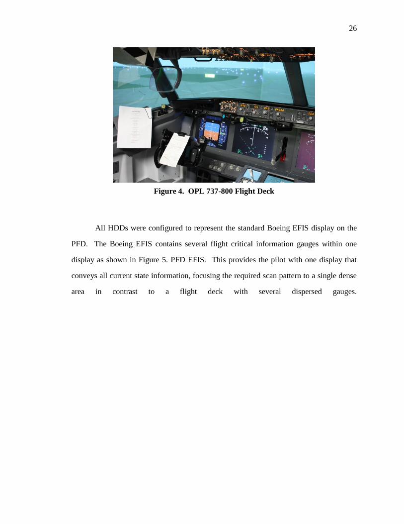
Figure 4. OPL 737-800 Flight Deck
All HDDs were configured to represent the standard Boeing EFIS display on the
PFD. The Boeing EFIS contains several flight critical information gauges within one
display as shown in Figure 5. PFD EFIS. This provides the pilot with one display that
conveys all current state information, focusing the required scan pattern to a single dense
area in contrast to a flight deck with several dispersed gauges.
27
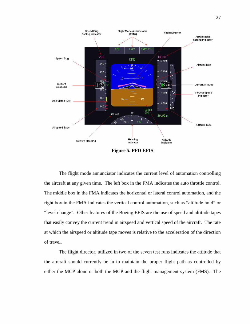
Figure 5. PFD EFIS
The flight mode annunciator indicates the current level of automation controlling
the aircraft at any given time. The left box in the FMA indicates the auto throttle control.
The middle box in the FMA indicates the horizontal or lateral control automation, and the
right box in the FMA indicates the vertical control automation, such as “altitude hold” or
“level change”. Other features of the Boeing EFIS are the use of speed and altitude tapes
that easily convey the current trend in airspeed and vertical speed of the aircraft. The rate
at which the airspeed or altitude tape moves is relative to the acceleration of the direction
of travel.
The flight director, utilized in two of the seven test runs indicates the attitude that
the aircraft should currently be in to maintain the proper flight path as controlled by
either the MCP alone or both the MCP and the flight management system (FMS). The
28
pilot simply controls the aircraft attitude indicator behind the flight director and the
proper flight path will be achieved.
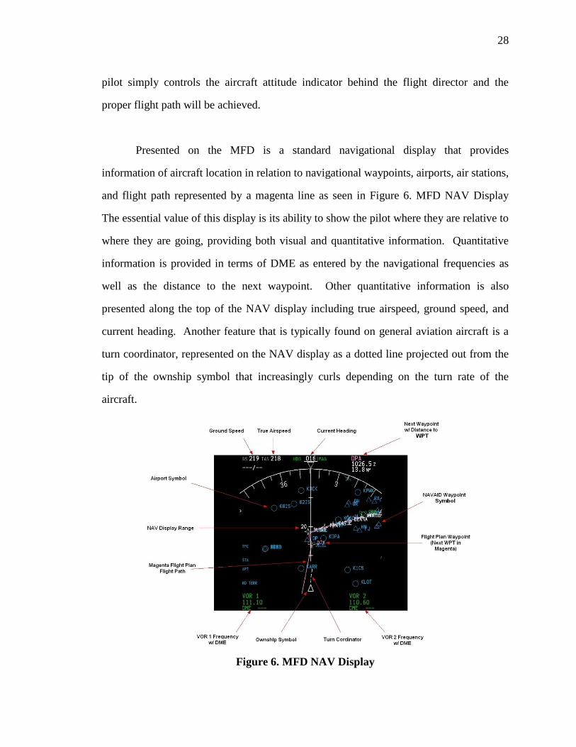
Presented on the MFD is a standard navigational display that provides
information of aircraft location in relation to navigational waypoints, airports, air stations,
and flight path represented by a magenta line as seen in Figure 6. MFD NAV Display
The essential value of this display is its ability to show the pilot where they are relative to
where they are going, providing both visual and quantitative information. Quantitative
information is provided in terms of DME as entered by the navigational frequencies as
well as the distance to the next waypoint. Other quantitative information is also
presented along the top of the NAV display including true airspeed, ground speed, and
current heading. Another feature that is typically found on general aviation aircraft is a
turn coordinator, represented on the NAV display as a dotted line projected out from the
tip of the ownship symbol that increasingly curls depending on the turn rate of the
aircraft.
Figure 6. MFD NAV Display
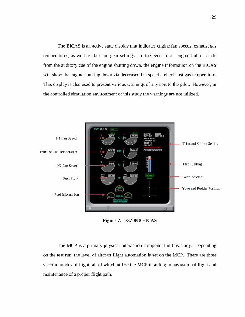
29
The EICAS is an active state display that indicates engine fan speeds, exhaust gas
temperatures, as well as flap and gear settings. In the event of an engine failure, aside
from the auditory cue of the engine shutting down, the engine information on the EICAS
will show the engine shutting down via decreased fan speed and exhaust gas temperature.
This display is also used to present various warnings of any sort to the pilot. However, in
the controlled simulation environment of this study the warnings are not utilized.
Figure 7. 737-800 EICAS
The MCP is a primary physical interaction component in this study. Depending
on the test run, the level of aircraft flight automation is set on the MCP. There are three
specific modes of flight, all of which utilize the MCP in aiding in navigational flight and
maintenance of a proper flight path.
N1 Fan Speed
Exhaust Gas Temperature
N2 Fan Speed
Trim and Spoiler Setting
Fuel Information
Fuel Flow
Flaps Setting
Gear Indicator
Yoke and Rudder Position
30
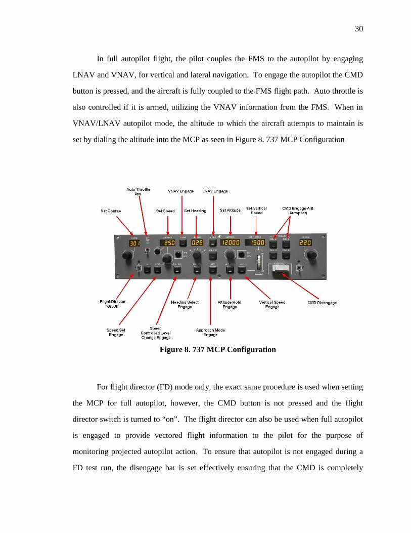
In full autopilot flight, the pilot couples the FMS to the autopilot by engaging
LNAV and VNAV, for vertical and lateral navigation. To engage the autopilot the CMD
button is pressed, and the aircraft is fully coupled to the FMS flight path. Auto throttle is
also controlled if it is armed, utilizing the VNAV information from the FMS. When in
VNAV/LNAV autopilot mode, the altitude to which the aircraft attempts to maintain is
set by dialing the altitude into the MCP as seen in Figure 8. 737 MCP Configuration
Figure 8. 737 MCP Configuration
For flight director (FD) mode only, the exact same procedure is used when setting
the MCP for full autopilot, however, the CMD button is not pressed and the flight
director switch is turned to “on”. The flight director can also be used when full autopilot
is engaged to provide vectored flight information to the pilot for the purpose of
monitoring projected autopilot action. To ensure that autopilot is not engaged during a
FD test run, the disengage bar is set effectively ensuring that the CMD is completely
31
uncoupled to the flight controls. The auto-throttle is still engaged as long as the auto-
throttle switched is turned on.
When intercepting the localizer on an approach to a runway equipped with a
localizer, the pilot switches the aircraft to approach (APP) mode by pressing the approach
mode button, changing the source of information that the MCP receives flight path
information from. Approach mode uses navigational frequencies set either manually by
the pilot or automatically by the FMS. The frequency is designated for a specific runway
localizer that the MCP then searches for. The FMA will indicate when the MCP has
locked onto the localizer and will then control the aircraft to follow the localizer to the
runway regardless of what the heading or altitude is set to. The auto throttle is still
controlled by the set speed on the MCP when in approach mode.
For manual flight, no engage buttons are activated on the MCP, including the FD
switch turned to off, the auto-throttle arm switch turned off and the disengage bar
switched down to the off position. All speed, heading, course, and altitude set indicators
can still be manipulated to set the “bugs” on the PFD and MFD. This is useful for pilots
to see where the current aircraft state is relative to where it should be as set on the MCP.
This is only accurate if the pilot takes the time to set the MCP for the proper speed,
altitude and headings appropriately. No other guidance is provided in this mode.
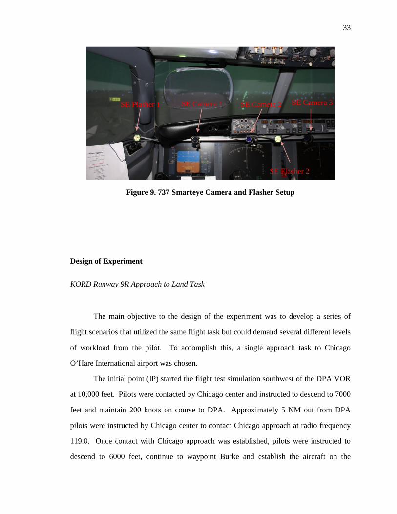
Smarteye Eye Tracking System
To obtain quantitative eye tracking data, a Smarteye eye tracking system was
installed and optimized inside the OPL’s 737-800 simulator. The Smarteye eye tracker is
a remote eye tracking system that uses facial recognition to calculate the position of
defined points on a subjects head relative to the calibrated position of 2 or more cameras.
32
The camera’s use the facial features to locate the corners of each of the subject’s eyes and
digitally zooms to enhance the image of the eye.
To calculate eye gaze vectors from the head origin, infrared led’s project infrared
light onto the pilots face, illuminating the pilots face as well as creating two ocular
reflections; a static corneal reflection and a moving pupil reflection that moves in
conjunction with eye movements. By triangulating the angular difference between the
corneal reflection and pupil reflection, the Smarteye eye tracking system can create a
vector between the two points to create an eye gaze vector originating from the corneal
reflection at the center of the subject’s eyes.
The 737 flight deck utilized a 3 camera system to achieve the visual angle of eye
tracking necessary to capture the test pilots’ gaze across the flight deck areas of interest.
From the test pilots used in this study, the Smarteye system was optimized to achieve an
average overall vector resolution down to approximately 1angular degree, and no greater
than 2 angular degrees. From the standard head position of each pilot, a length of about
three feet separated most areas of interest from the pilots’ eyes, giving an average overall
gaze vector resolution of approximately 0.63 inches across the flight deck. This
optimization allowed research to be conducted for much smaller areas of interest while
retaining consistently accurate and precise eye tracking data.
33
Figure 9. 737 Smarteye Camera and Flasher Setup
Design of Experiment
KORD Runway 9R Approach to Land Task
The main objective to the design of the experiment was to develop a series of
flight scenarios that utilized the same flight task but could demand several different levels
of workload from the pilot. To accomplish this, a single approach task to Chicago
O’Hare International airport was chosen.
The initial point (IP) started the flight test simulation southwest of the DPA VOR
at 10,000 feet. Pilots were contacted by Chicago center and instructed to descend to 7000
feet and maintain 200 knots on course to DPA. Approximately 5 NM out from DPA
pilots were instructed by Chicago center to contact Chicago approach at radio frequency
119.0. Once contact with Chicago approach was established, pilots were instructed to
descend to 6000 feet, continue to waypoint Burke and establish the aircraft on the
SE Camera 1 SE Camera 2 SE Camera 3 SE Flasher 1
SE Flasher 2
34
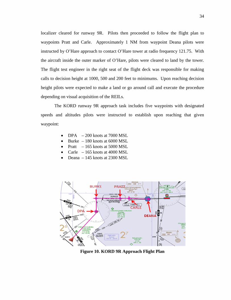
localizer cleared for runway 9R. Pilots then proceeded to follow the flight plan to
waypoints Pratt and Carle. Approximately 1 NM from waypoint Deana pilots were
instructed by O’Hare approach to contact O’Hare tower at radio frequency 121.75. With
the aircraft inside the outer marker of O’Hare, pilots were cleared to land by the tower.
The flight test engineer in the right seat of the flight deck was responsible for making
calls to decision height at 1000, 500 and 200 feet to minimums. Upon reaching decision
height pilots were expected to make a land or go around call and execute the procedure
depending on visual acquisition of the REILs.
The KORD runway 9R approach task includes five waypoints with designated
speeds and altitudes pilots were instructed to establish upon reaching that given
waypoint:
• DPA – 200 knots at 7000 MSL • Burke – 180 knots at 6000 MSL • Pratt – 165 knots at 5000 MSL • Carle – 165 knots at 4000 MSL • Deana – 145 knots at 2300 MSL
Figure 10. KORD 9R Approach Flight Plan
35
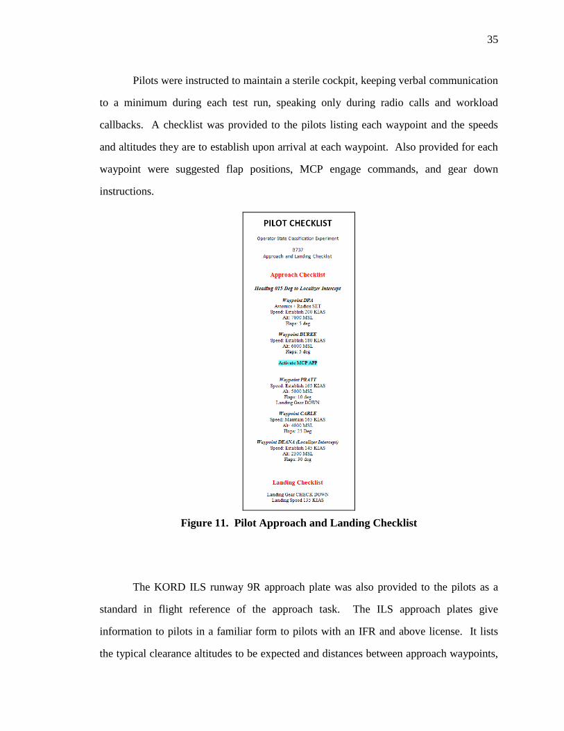
Pilots were instructed to maintain a sterile cockpit, keeping verbal communication
to a minimum during each test run, speaking only during radio calls and workload
callbacks. A checklist was provided to the pilots listing each waypoint and the speeds
and altitudes they are to establish upon arrival at each waypoint. Also provided for each
waypoint were suggested flap positions, MCP engage commands, and gear down
instructions.
Figure 11. Pilot Approach and Landing Checklist
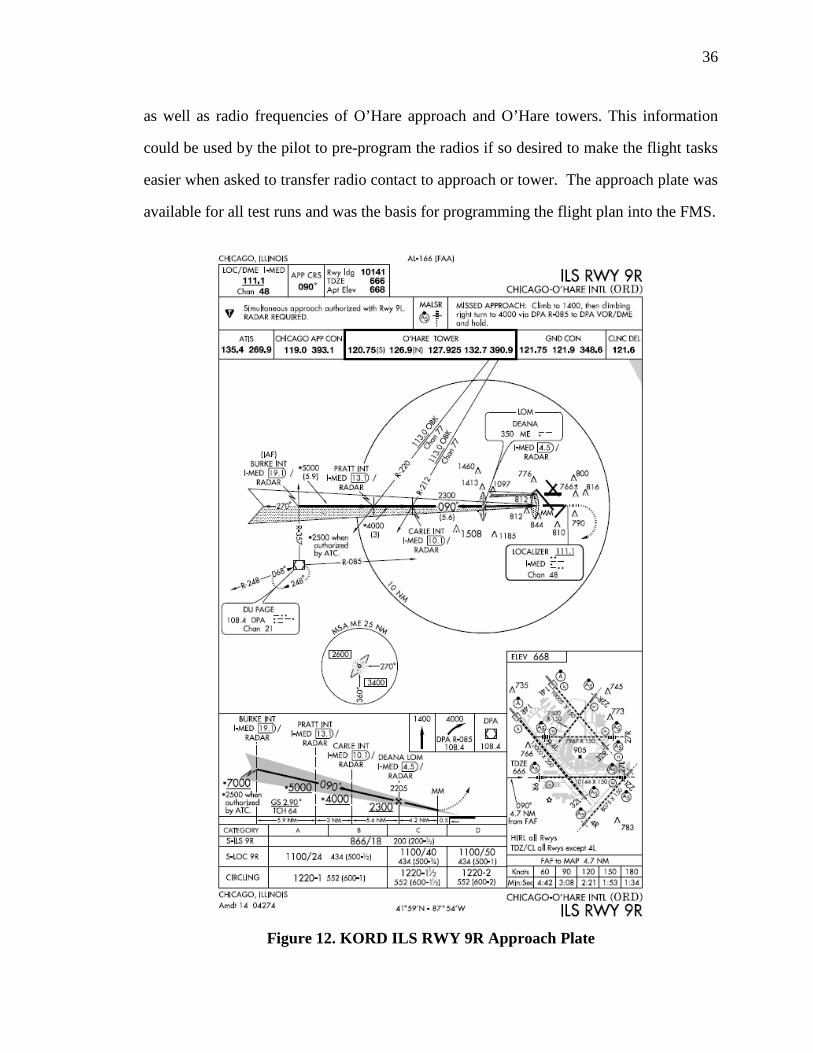
The KORD ILS runway 9R approach plate was also provided to the pilots as a
standard in flight reference of the approach task. The ILS approach plates give
information to pilots in a familiar form to pilots with an IFR and above license. It lists
the typical clearance altitudes to be expected and distances between approach waypoints,
36
as well as radio frequencies of O’Hare approach and O’Hare towers. This information
could be used by the pilot to pre-program the radios if so desired to make the flight tasks
easier when asked to transfer radio contact to approach or tower. The approach plate was
available for all test runs and was the basis for programming the flight plan into the FMS.
Figure 12. KORD ILS RWY 9R Approach Plate
37
Test Conditions
Two methods to drive workload to show high-low workload contrasts were implemented:
• Visibility condition – CAT II and CAT III o Land or Go Around condition
• Level of automation o Full Autopilot and Auto-throttle o FD guidance and Auto-throttle o Manual approach with localizer course and glide slope guidance only
For the visibility condition, outside visuals were controlled to be set to CAT II
visibility, with no greater than 0.3 NM visibility, or set to CAT III, with no greater than
0.1 NM visibility. The threshold of visibility between the two visibility conditions forced
the pilot to make a land-no land decision at decision height at 200 feet AGL. Upon
reaching 200 feet AGL, federal air regulations (FARs) state that the pilot must be able to
see the runway end indicator lights (REILs) to continue to land. If the pilot cannot see
the REILs at 200 feet above the runway, the pilot must execute a go-around. If the pilot
is able to see the REILs at 200 feet AGL, then the pilot was to proceed to 100 feet AGL
where they are required by FARs to make visual contact with the end of the runway to
continue to land. The variance in visibility conditions made no impact on the 100 foot
AGL decision height. The difficulty for the pilot is found in the time for which the
decision to land must be made and to maintain the proper flight path to the runway with
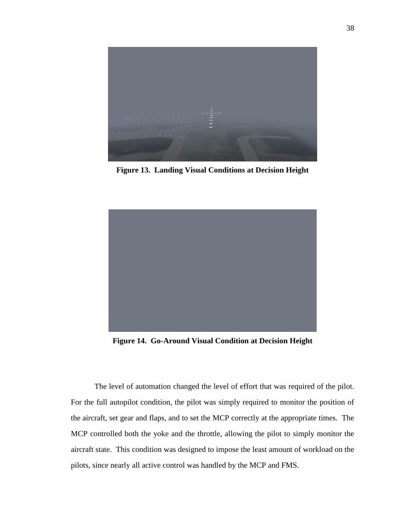
no outside visuals obtaining guidance strictly from the HDDs.
38
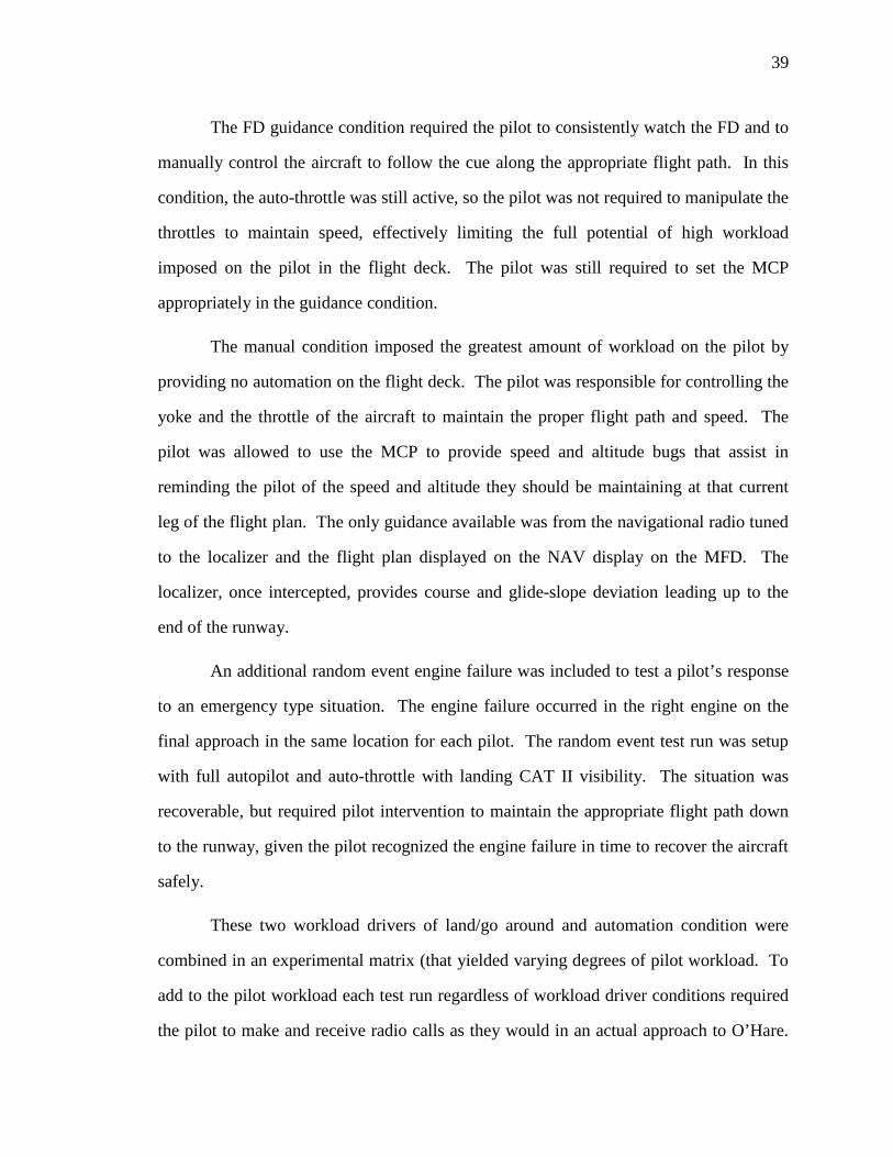
Figure 13. Landing Visual Conditions at Decision Height
Figure 14. Go-Around Visual Condition at Decision Height
The level of automation changed the level of effort that was required of the pilot.
For the full autopilot condition, the pilot was simply required to monitor the position of
the aircraft, set gear and flaps, and to set the MCP correctly at the appropriate times. The
MCP controlled both the yoke and the throttle, allowing the pilot to simply monitor the
aircraft state. This condition was designed to impose the least amount of workload on the
pilots, since nearly all active control was handled by the MCP and FMS.
39
The FD guidance condition required the pilot to consistently watch the FD and to
manually control the aircraft to follow the cue along the appropriate flight path. In this
condition, the auto-throttle was still active, so the pilot was not required to manipulate the
throttles to maintain speed, effectively limiting the full potential of high workload
imposed on the pilot in the flight deck. The pilot was still required to set the MCP
appropriately in the guidance condition.
The manual condition imposed the greatest amount of workload on the pilot by
providing no automation on the flight deck. The pilot was responsible for controlling the
yoke and the throttle of the aircraft to maintain the proper flight path and speed. The
pilot was allowed to use the MCP to provide speed and altitude bugs that assist in
reminding the pilot of the speed and altitude they should be maintaining at that current
leg of the flight plan. The only guidance available was from the navigational radio tuned
to the localizer and the flight plan displayed on the NAV display on the MFD. The
localizer, once intercepted, provides course and glide-slope deviation leading up to the
end of the runway.
An additional random event engine failure was included to test a pilot’s response
to an emergency type situation. The engine failure occurred in the right engine on the
final approach in the same location for each pilot. The random event test run was setup
with full autopilot and auto-throttle with landing CAT II visibility. The situation was
recoverable, but required pilot intervention to maintain the appropriate flight path down
to the runway, given the pilot recognized the engine failure in time to recover the aircraft
safely.
These two workload drivers of land/go around and automation condition were
combined in an experimental matrix (that yielded varying degrees of pilot workload. To
add to the pilot workload each test run regardless of workload driver conditions required
the pilot to make and receive radio calls as they would in an actual approach to O’Hare.
40
The pilot was given clearance to waypoints at specific altitudes and speeds. The pilot was
also instructed to change radio frequencies when told to switch from Chicago center to
O’Hare approach, and again from O’Hare approach to O’Hare tower. Pilots were
instructed to read back their instructions as they would typically in standard flight.
A complex hold call was given to pilots on one of the seven test runs.
Instructions were given to the pilot not to execute the hold, but to retain the call in
memory for 30 seconds and to read them back at the end of the 30 second memory
period. This was intended to further increase pilot workload by distracting them
cognitively. Correct or incorrect response information was collected by the flight test
engineers. The hold call was presented in random order between the various test pilots.
Subjective Workload Assessment
To assess pilot workload, three subjective scales were utilized for each test run; A
Bedford workload scale, SART, a situational awareness assessment analysis
questionnaire, and the NASA-TLX subject demand assessment. The subjective workload
assessment scores provide the baseline connection between the quantitative data results
and the pilot’s perceived workload for each test run condition. The quantitative data
results from the eye tracking metrics will be analyzed and regressed against the pilots
subjective workload assessments.
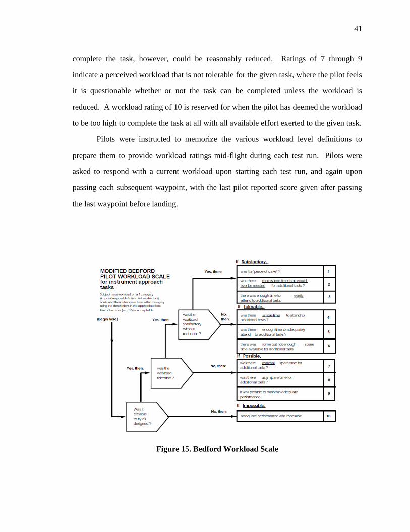
The Bedford workload scale is a 1-10 workload rating assessing the current
workload perceived by the pilot. The scale is a decision tree that attempts to minimize
the workload reporting differences across pilots. A pilot answers a series of questions to
eventually come to a concluding Bedford workload rating as seen in Figure 15. Bedford
Workload Scale Workload ratings of 1 through 3 are scores of satisfactory perceived
workload. Ratings of 4 through 6 indicate a perceived workload that was tolerable to
41
complete the task, however, could be reasonably reduced. Ratings of 7 through 9
indicate a perceived workload that is not tolerable for the given task, where the pilot feels
it is questionable whether or not the task can be completed unless the workload is
reduced. A workload rating of 10 is reserved for when the pilot has deemed the workload
to be too high to complete the task at all with all available effort exerted to the given task.
Pilots were instructed to memorize the various workload level definitions to
prepare them to provide workload ratings mid-flight during each test run. Pilots were
asked to respond with a current workload upon starting each test run, and again upon
passing each subsequent waypoint, with the last pilot reported score given after passing
the last waypoint before landing.
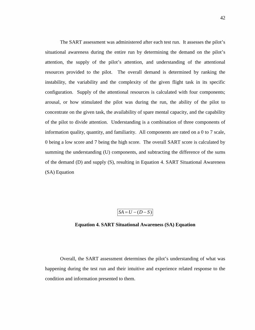
Figure 15. Bedford Workload Scale
42
The SART assessment was administered after each test run. It assesses the pilot’s
situational awareness during the entire run by determining the demand on the pilot’s
attention, the supply of the pilot’s attention, and understanding of the attentional
resources provided to the pilot. The overall demand is determined by ranking the
instability, the variability and the complexity of the given flight task in its specific
configuration. Supply of the attentional resources is calculated with four components;
arousal, or how stimulated the pilot was during the run, the ability of the pilot to
concentrate on the given task, the availability of spare mental capacity, and the capability
of the pilot to divide attention. Understanding is a combination of three components of
information quality, quantity, and familiarity. All components are rated on a 0 to 7 scale,
0 being a low score and 7 being the high score. The overall SART score is calculated by
summing the understanding (U) components, and subtracting the difference of the sums
of the demand (D) and supply (S), resulting in Equation 4. SART Situational Awareness
(SA) Equation
)( SDUSA −−=
Equation 4. SART Situational Awareness (SA) Equation
Overall, the SART assessment determines the pilot’s understanding of what was
happening during the test run and their intuitive and experience related response to the
condition and information presented to them.
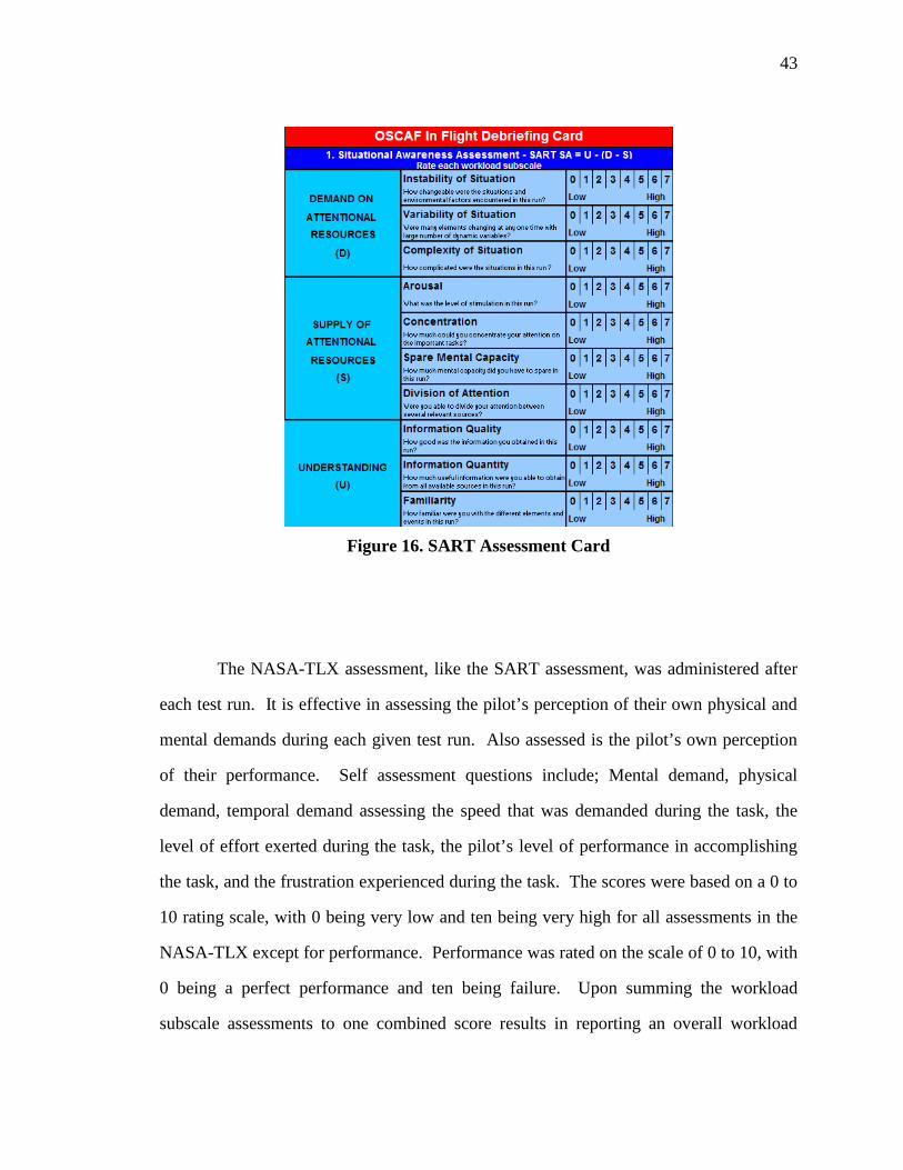
43
Figure 16. SART Assessment Card
The NASA-TLX assessment, like the SART assessment, was administered after
each test run. It is effective in assessing the pilot’s perception of their own physical and
mental demands during each given test run. Also assessed is the pilot’s own perception
of their performance. Self assessment questions include; Mental demand, physical
demand, temporal demand assessing the speed that was demanded during the task, the
level of effort exerted during the task, the pilot’s level of performance in accomplishing
the task, and the frustration experienced during the task. The scores were based on a 0 to
10 rating scale, with 0 being very low and ten being very high for all assessments in the
NASA-TLX except for performance. Performance was rated on the scale of 0 to 10, with
0 being a perfect performance and ten being failure. Upon summing the workload
subscale assessments to one combined score results in reporting an overall workload
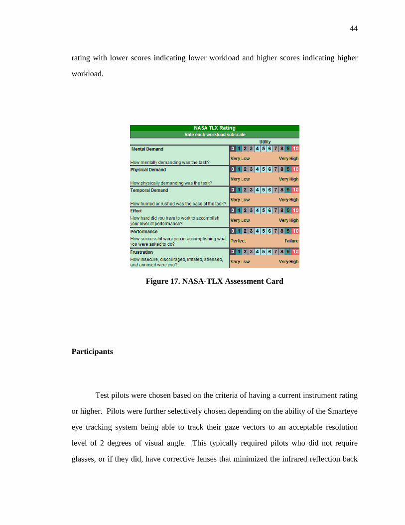
44
rating with lower scores indicating lower workload and higher scores indicating higher
workload.
Figure 17. NASA-TLX Assessment Card
Participants
Test pilots were chosen based on the criteria of having a current instrument rating
or higher. Pilots were further selectively chosen depending on the ability of the Smarteye
eye tracking system being able to track their gaze vectors to an acceptable resolution
level of 2 degrees of visual angle. This typically required pilots who did not require
glasses, or if they did, have corrective lenses that minimized the infrared reflection back
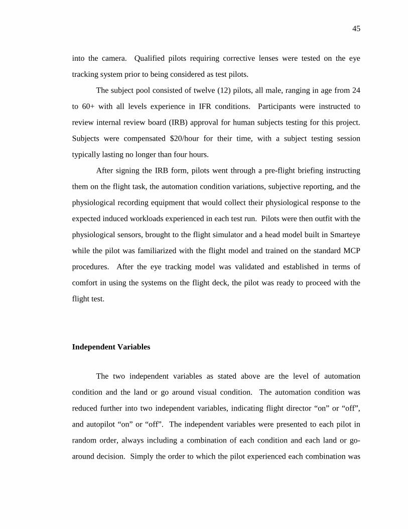
45
into the camera. Qualified pilots requiring corrective lenses were tested on the eye
tracking system prior to being considered as test pilots.
The subject pool consisted of twelve (12) pilots, all male, ranging in age from 24
to 60+ with all levels experience in IFR conditions. Participants were instructed to
review internal review board (IRB) approval for human subjects testing for this project.
Subjects were compensated $20/hour for their time, with a subject testing session
typically lasting no longer than four hours.
After signing the IRB form, pilots went through a pre-flight briefing instructing
them on the flight task, the automation condition variations, subjective reporting, and the
physiological recording equipment that would collect their physiological response to the
expected induced workloads experienced in each test run. Pilots were then outfit with the
physiological sensors, brought to the flight simulator and a head model built in Smarteye
while the pilot was familiarized with the flight model and trained on the standard MCP
procedures. After the eye tracking model was validated and established in terms of
comfort in using the systems on the flight deck, the pilot was ready to proceed with the
flight test.
Independent Variables
The two independent variables as stated above are the level of automation
condition and the land or go around visual condition. The automation condition was
reduced further into two independent variables, indicating flight director “on” or “off”,
and autopilot “on” or “off”. The independent variables were presented to each pilot in
random order, always including a combination of each condition and each land or go-
around decision. Simply the order to which the pilot experienced each combination was
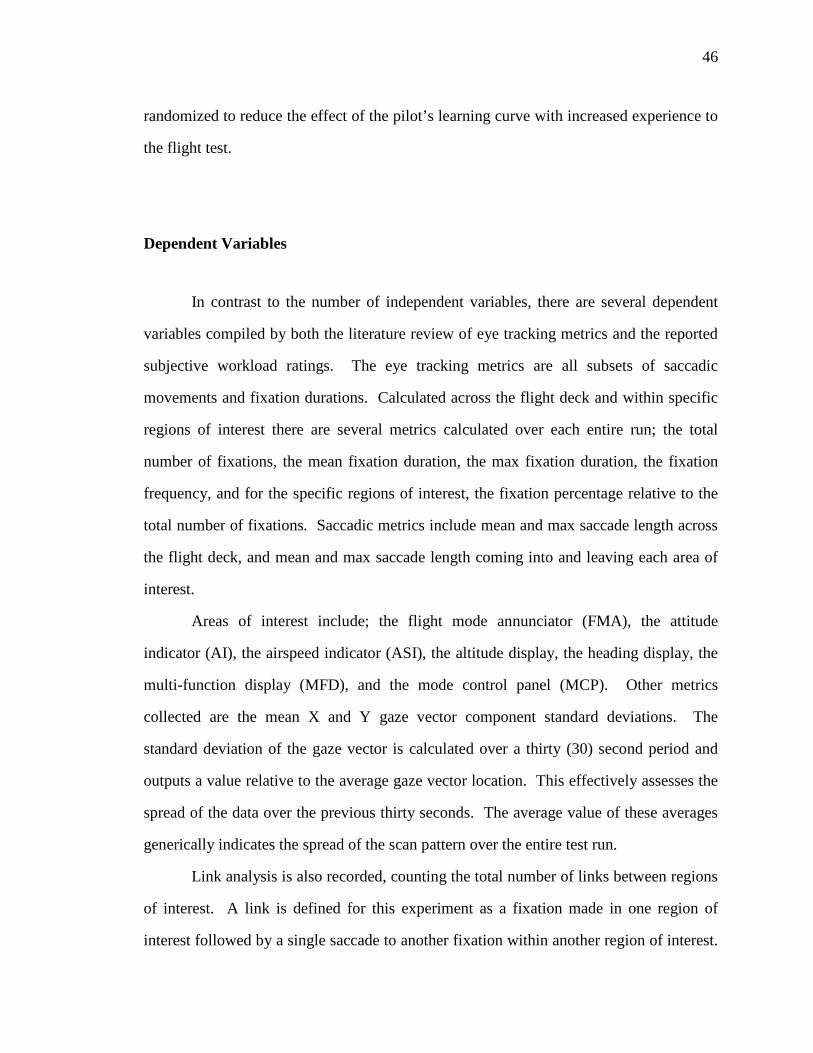
46
randomized to reduce the effect of the pilot’s learning curve with increased experience to
the flight test.
Dependent Variables
In contrast to the number of independent variables, there are several dependent
variables compiled by both the literature review of eye tracking metrics and the reported
subjective workload ratings. The eye tracking metrics are all subsets of saccadic
movements and fixation durations. Calculated across the flight deck and within specific
regions of interest there are several metrics calculated over each entire run; the total
number of fixations, the mean fixation duration, the max fixation duration, the fixation
frequency, and for the specific regions of interest, the fixation percentage relative to the
total number of fixations. Saccadic metrics include mean and max saccade length across
the flight deck, and mean and max saccade length coming into and leaving each area of
interest.
Areas of interest include; the flight mode annunciator (FMA), the attitude
indicator (AI), the airspeed indicator (ASI), the altitude display, the heading display, the
multi-function display (MFD), and the mode control panel (MCP). Other metrics
collected are the mean X and Y gaze vector component standard deviations. The
standard deviation of the gaze vector is calculated over a thirty (30) second period and
outputs a value relative to the average gaze vector location. This effectively assesses the
spread of the data over the previous thirty seconds. The average value of these averages
generically indicates the spread of the scan pattern over the entire test run.
Link analysis is also recorded, counting the total number of links between regions
of interest. A link is defined for this experiment as a fixation made in one region of
interest followed by a single saccade to another fixation within another region of interest.
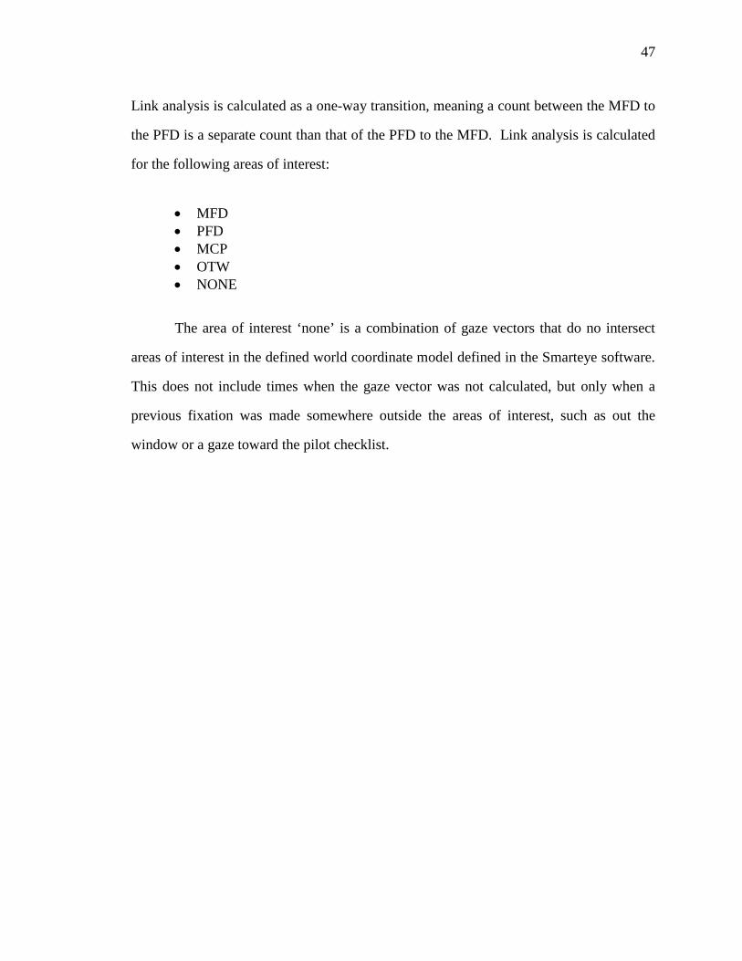
47
Link analysis is calculated as a one-way transition, meaning a count between the MFD to
the PFD is a separate count than that of the PFD to the MFD. Link analysis is calculated
for the following areas of interest:
• MFD • PFD • MCP • OTW • NONE
The area of interest ‘none’ is a combination of gaze vectors that do no intersect
areas of interest in the defined world coordinate model defined in the Smarteye software.
This does not include times when the gaze vector was not calculated, but only when a
previous fixation was made somewhere outside the areas of interest, such as out the
window or a gaze toward the pilot checklist.
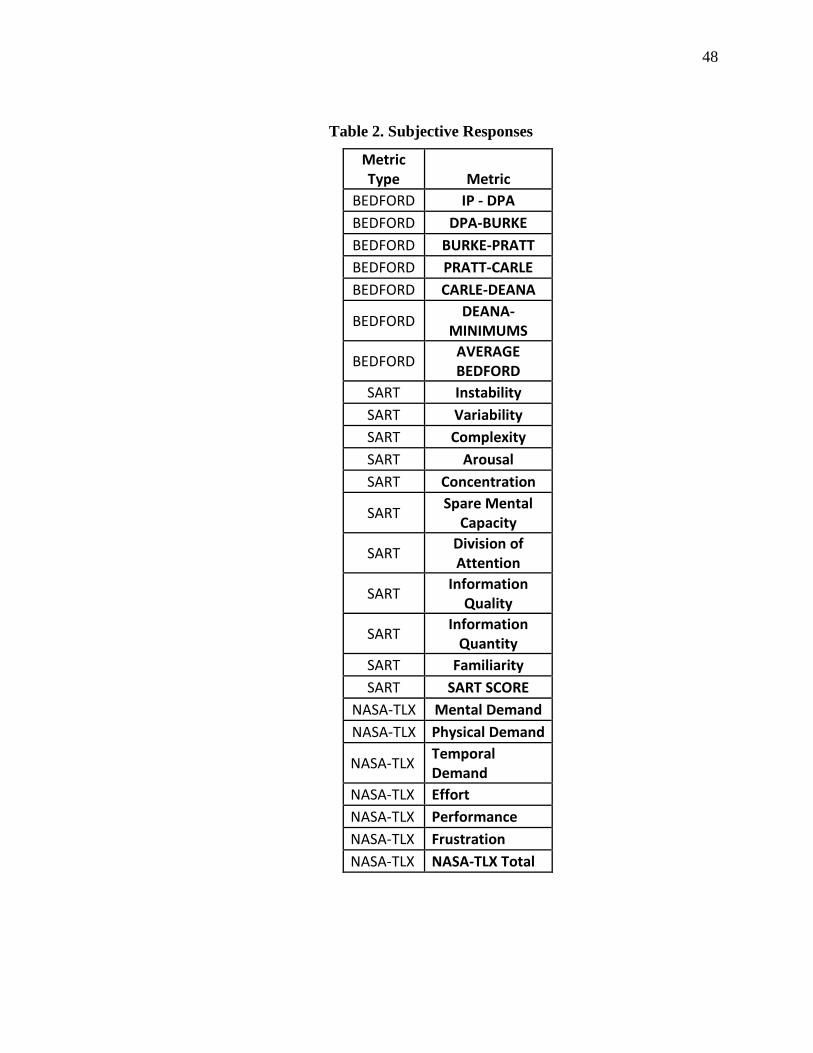
48
Table 2. Subjective Responses
Metric
Type Metric
BEDFORD IP - DPA
BEDFORD DPA-BURKE
BEDFORD BURKE-PRATT
BEDFORD PRATT-CARLE
BEDFORD CARLE-DEANA
BEDFORD DEANA-
MINIMUMS
BEDFORD AVERAGE
BEDFORD
SART Instability
SART Variability
SART Complexity
SART Arousal
SART Concentration
SART Spare Mental
Capacity
SART Division of
Attention
SART Information
Quality
SART Information
Quantity
SART Familiarity
SART SART SCORE
NASA-TLX Mental Demand
NASA-TLX Physical Demand
NASA-TLX Temporal
Demand
NASA-TLX Effort
NASA-TLX Performance
NASA-TLX Frustration
NASA-TLX NASA-TLX Total
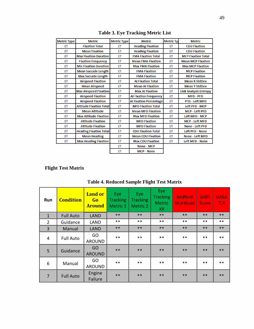
49
Table 3. Eye Tracking Metric List
Flight Test Matrix
Table 4. Reduced Sample Flight Test Matrix
Run Condition
Land or
Go
Around
Eye
Tracking
Metric 1
Eye
Tracking
Metric 2
Eye
Tracking
Metric
XX
Bedford
Workload
SART
Score
NASA
TLX
1 Full Auto LAND ** ** ** ** ** **
2 Guidance LAND ** ** ** ** ** **
3 Manual LAND ** ** ** ** ** **
4 Full Auto GO
AROUND ** ** ** ** ** **
5 Guidance GO
AROUND ** ** ** ** ** **
6 Manual GO
AROUND ** ** ** ** ** **
7 Full Auto Engine
Failure ** ** ** ** ** **
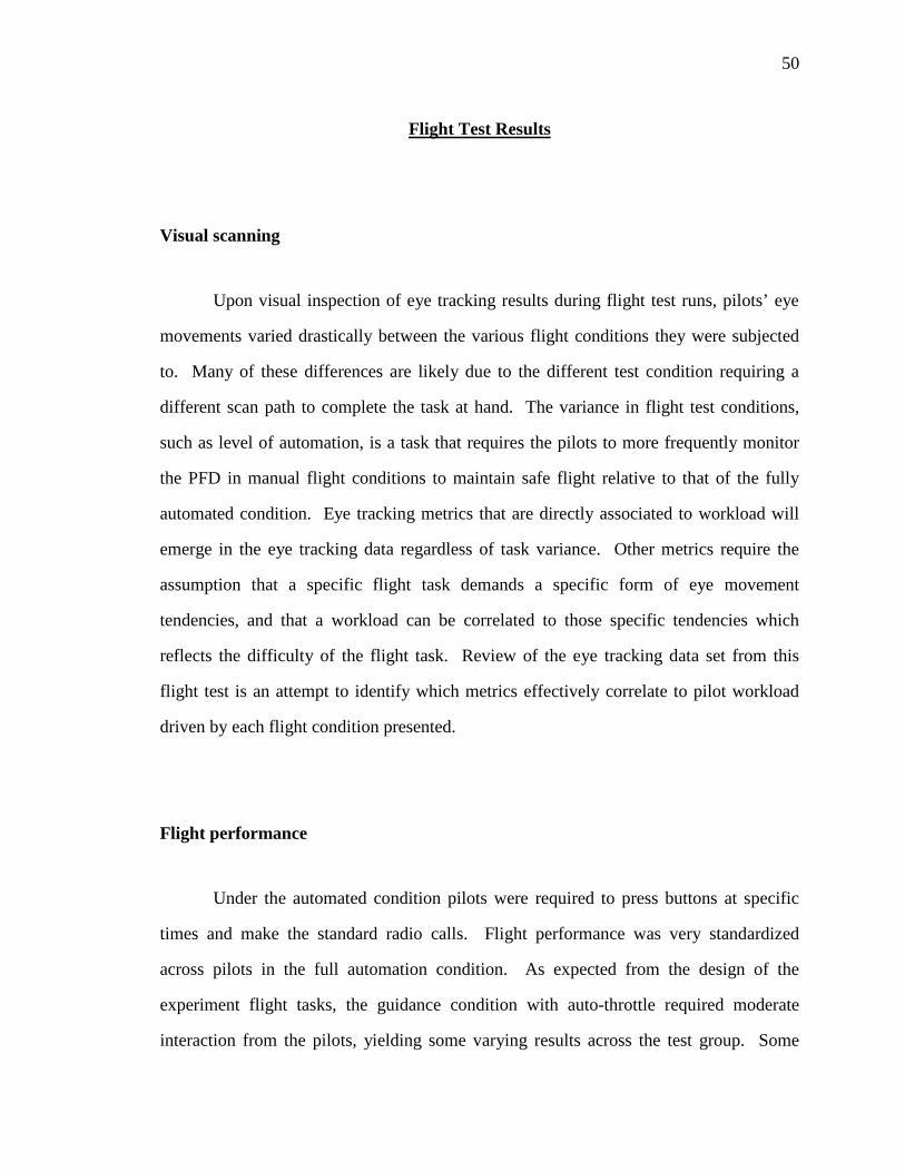
50
Flight Test Results
Visual scanning
Upon visual inspection of eye tracking results during flight test runs, pilots’ eye
movements varied drastically between the various flight conditions they were subjected
to. Many of these differences are likely due to the different test condition requiring a
different scan path to complete the task at hand. The variance in flight test conditions,
such as level of automation, is a task that requires the pilots to more frequently monitor
the PFD in manual flight conditions to maintain safe flight relative to that of the fully
automated condition. Eye tracking metrics that are directly associated to workload will
emerge in the eye tracking data regardless of task variance. Other metrics require the
assumption that a specific flight task demands a specific form of eye movement
tendencies, and that a workload can be correlated to those specific tendencies which
reflects the difficulty of the flight task. Review of the eye tracking data set from this
flight test is an attempt to identify which metrics effectively correlate to pilot workload
driven by each flight condition presented.
Flight performance
Under the automated condition pilots were required to press buttons at specific
times and make the standard radio calls. Flight performance was very standardized
across pilots in the full automation condition. As expected from the design of the
experiment flight tasks, the guidance condition with auto-throttle required moderate
interaction from the pilots, yielding some varying results across the test group. Some
51
pilots who had experience utilizing a flight director performed the flight tasks with
greater ease than those pilots experiencing it for the first time that day. This experience
related difference yielded varying subjective workload feedback from the pilots. The
highest reported workloads did come from the manual flight test condition, when pilots
were required to control both the attitude of the aircraft and the speed, requiring the most
mental cognition from the pilot to maintain the specified aircraft state at the right times
and locations.
Several times pilots would find themselves off-course due to the high mental
demand required by several systems at once, such as thrust level, attitude adjustment and
radio communication. Diverging oscillations in recovering the flight path intercept was
very typical across pilots in the manual condition, ultimately driving the pilots’ workload
to higher levels on the Bedford workload scale.
Flight Test Conclusions
The flight test was run as expected with no changes necessary from the first pilot
to the last. Like any other experiment, system malfunctions imposed minor setbacks in
timing during some of the runs, however, did not affect the data in any significant way.
Pilot responses indicated significant workload variance upon initial inspection of
subjective results and verbal pilot feedback. Collected data integrity was actively
monitored during all flight test runs.

52
CHAPTER 4.
DATA ANALYSIS AND ALGORITHM DEVELOPMENT
Data Set
The data was collected and stored on removable drives on the input/output system
(IOS) computer connected to the flight simulator. Several systems were connected to the
data collection IOS that were used for physiological assessment as well as the simulator
command components mentioned in chapter 3. Several buses collected several variables
useful in the data analysis of this study, as well as other studies with an interest in
operator state classification, shown in Table 5. IOS Collection Data.
Data collection included several components not pertinent to eye tracking, but
overall operator state through several channels of physiological output of the subject.
The IOS included a ‘Stamp’ to separate out each data point by frame number and by
time, ‘Run Info’ to record which data set belonged to which subject and task that each
subject was performing, aircraft state information, instrumentation recording pilot control
inputs, nexus physiological measurement data, recording ECG for heart-rate, respiration
rate and depth, EMG collecting right arm deltoid flexion to collect MCP button presses
and throttle manipulation, and the eye tracking output information from the Smarteye
system described in greater detail in the Smarteye Eye Tracking System section of chapter
3.

53
The quality of the data set is very robust for all eye tracking metrics analyzed
across the entire flight deck. However, pre-processing software output did not provide
consistent data for all aforementioned regions of interest. Altitude, heading, MFD, speed,
out the window (OTW), and MCP regions were captured and entered into the data set.
Attitude indicator and FMA were not collected due to errors in region labeling during
data collection and will be analyzed upon further investigation of the data set in future
research initiatives. The attitude indicator and FMA were not included in the regression
and ANOVA analysis of this thesis.
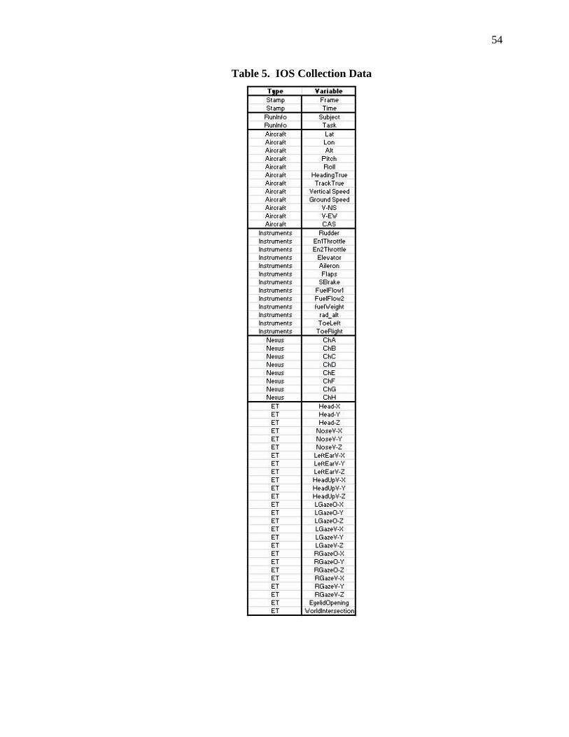
54
Table 5. IOS Collection Data

55
Analysis of the subjective results crossed with the testing conditions indicated that
the varying test conditions (Level of Automation, Land/Go Around) did yield a variance
in induced workload. Workload was assessed in real time using the Bedford workload
scale, and post-run using the SART situational awareness assessment and the NASA-
TLX. Analysis shows that all assessments correlate together as expected and are
indicative of the pilot’s perceived performance and associative workload in each test run.
AVERAGE BEDFO
RD
Land or Go Around
Condition
LAND
GO AROUND
Engine Failure
Manual
Guidance
Full Auto
Manual
Guidance
Full Auto
Manual
Guidance
Ful l Auto
Manual
Guidance
Full Auto
10
9
8
7
6
5
4
3
2
1
Figure 18. Boxplot of Average Bedford Score vs. Land/Go-Around, Condition
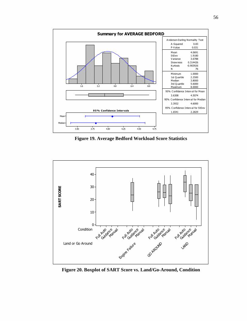
56
8.06.44.83.21.6
Median
Mean
4.754.504.254.003.753.50
1st Q uartile 2.2500
Median 3.8000
3rd Q uartile 5.6000
Maximum 8.0000
3.6308 4.5074
3.3932 4.6000
1.6541 2.2829
A -Squared 0.83
P-V alue 0.031
Mean 4.0691
StDev 1.9180
V ariance 3.6788
Skewness 0.314426
Kurtosis -0.903926
N 76
Minimum 1.0000
A nderson-Darling Normality Test
95% C onfidence Interv al for Mean
95% C onfidence Interv al for Median
95% C onfidence Interv al for StDev95% Confidence Intervals
Summary for AVERAGE BEDFORD
Figure 19. Average Bedford Workload Score Statistics
SART SCORE
Land or Go Around
Condition
LAND
GO AROUND
Engine Failure
Manual
Guidance
Full Auto
Manual
Guidance
Full Auto
Manual
Guidance
Ful l Auto
Manual
Guidance
Full Auto
40
30
20
10
0
Figure 20. Boxplot of SART Score vs. Land/Go-Around, Condition
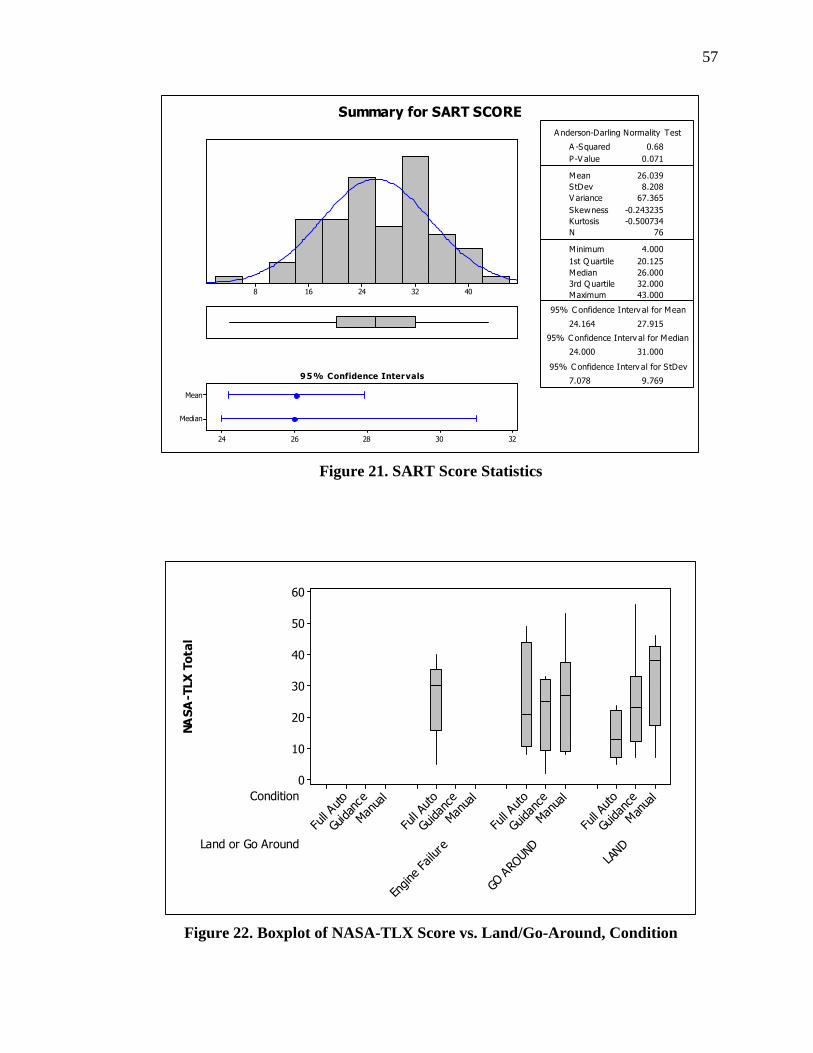
57
403224168
Median
Mean
3230282624
1st Q uartile 20.125
Median 26.000
3rd Quartile 32.000
Maximum 43.000
24.164 27.915
24.000 31.000
7.078 9.769
A -Squared 0.68
P-V alue 0.071
Mean 26.039
StDev 8.208
V ariance 67.365
Skewness -0.243235
Kurtosis -0.500734
N 76
Minimum 4.000
A nderson-Darling Normality Test
95% C onfidence Interv al for Mean
95% C onfidence Interv al for Median
95% C onfidence Interv al for StDev95% Confidence Intervals
Summary for SART SCORE
Figure 21. SART Score Statistics
NASA-TLX Total
Land or Go Around
Condition
LAND
GO AROUND
Engine Failure
Manual
Guidance
Full Auto
Manual
Guidance
Full Auto
Manual
Guidance
Full Auto
Manual
Guidance
Full Auto
60
50
40
30
20
10
0
Figure 22. Boxplot of NASA-TLX Score vs. Land/Go-Around, Condition
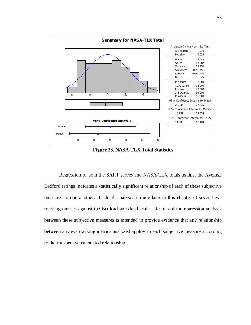
58
483624120
Median
Mean
302826242220
1st Q uartile 12.000
Median 22.500
3rd Q uartile 34.000
Maximum 56.000
20.936 27.235
18.932 29.034
11.886 16.404
A -Squared 0.79
P-V alue 0.038
Mean 24.086
StDev 13.782
V ariance 189.956
Skewness 0.284451
Kurtosis -0.882552
N 76
Minimum 2.000
A nderson-Darling Normality Test
95% C onfidence Interv al for Mean
95% C onfidence Interv al for Median
95% C onfidence Interv al for StDev95% Confidence Intervals
Summary for NASA-TLX Total
Figure 23. NASA-TLX Total Statistics
Regression of both the SART scores and NASA-TLX totals against the Average
Bedford ratings indicates a statistically significant relationship of each of these subjective
measures to one another. In depth analysis is done later in this chapter of several eye
tracking metrics against the Bedford workload scale. Results of the regression analysis
between these subjective measures is intended to provide evidence that any relationship
between any eye tracking metrics analyzed applies to each subjective measure according
to their respective calculated relationship.
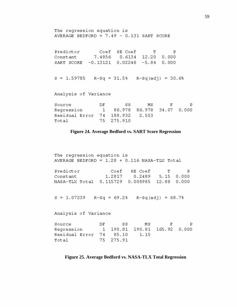
59
Figure 24. Average Bedford vs. SART Score Regression
Figure 25. Average Bedford vs. NASA-TLX Total Regression

60
Analysis Methodology
The raw data collected by the IOS was processed using preprocessing software
written to analyze the gaze vector output and to quantify it into both saccadic movements
and fixations. Fixations were defined in the preprocessing software as a series of eye
points falling within a 2 degree radius for greater than 300 milliseconds, with an outlier
tolerance of 100 milliseconds to filter noisy data points. Filtering creates a third
component, called an Orphan, which is a definition used to describe quick saccadic
movements under 100 milliseconds that break up an individual fixation. Fixations lasting
longer than 3 seconds were ignored in preprocessing calculations to filter out bad data.
Saccadic movements were counted as a component linking two fixations together, broken
down into distance in angular degrees.
To calculate the change in spatial spread of the fixation map/scan-path, the
standard deviation of the gaze vector in X and Y components over a period of 30 seconds
was determined and included as part of the output from the preprocessor. Larger
standard deviations in either direction indicate a larger spread in fixation density, and
therefore a higher level of entropy in the eye movement behavior of the subject, and a
change in the standard eye scan pattern.
The effort to discover a correlation between eye movement behavior and pilot
workload encounters two obstacles when analyzing the data set collected in this study;
the frequency of pilot subjective workload responses not being identical to the frequency
of collection data, creating the need for interpolation, a therefore assumed error, and
portions of data that misrepresent the actual behavior of the subjects eyes. The latter can
only be addressed by increasing the test population, which can be resolved by appending
future data onto this data set.
The first indicated problem is approached by organizing the raw data using two
methods; analysis of the 30 seconds prior to each waypoint to capture the eye movement
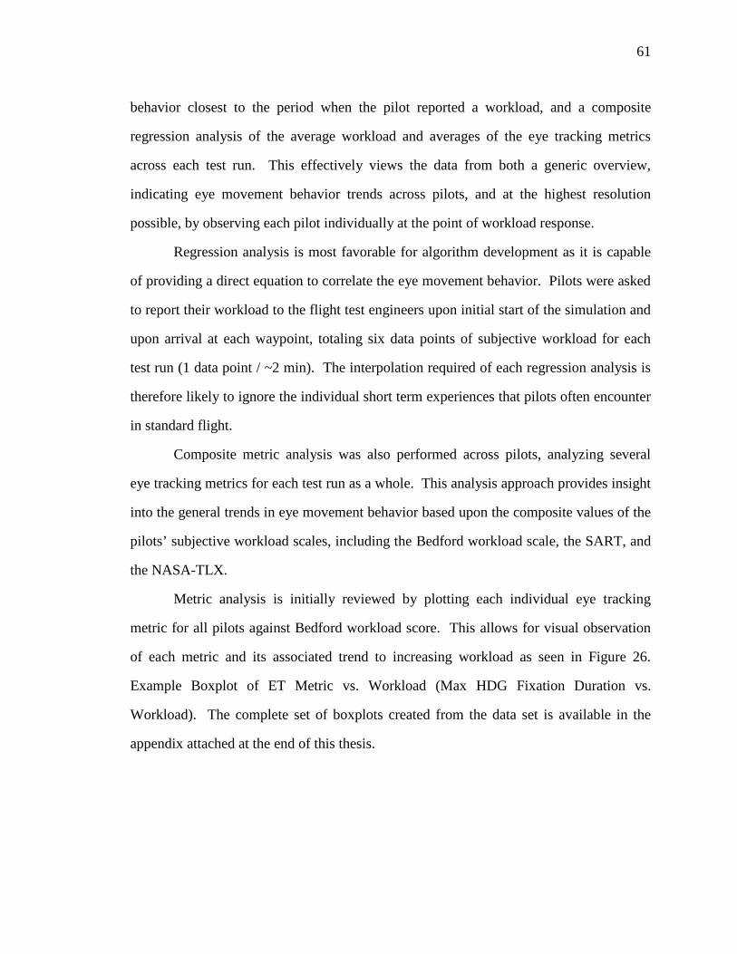
61
behavior closest to the period when the pilot reported a workload, and a composite
regression analysis of the average workload and averages of the eye tracking metrics
across each test run. This effectively views the data from both a generic overview,
indicating eye movement behavior trends across pilots, and at the highest resolution
possible, by observing each pilot individually at the point of workload response.
Regression analysis is most favorable for algorithm development as it is capable
of providing a direct equation to correlate the eye movement behavior. Pilots were asked
to report their workload to the flight test engineers upon initial start of the simulation and
upon arrival at each waypoint, totaling six data points of subjective workload for each
test run (1 data point / ~2 min). The interpolation required of each regression analysis is
therefore likely to ignore the individual short term experiences that pilots often encounter
in standard flight.
Composite metric analysis was also performed across pilots, analyzing several
eye tracking metrics for each test run as a whole. This analysis approach provides insight
into the general trends in eye movement behavior based upon the composite values of the
pilots’ subjective workload scales, including the Bedford workload scale, the SART, and
the NASA-TLX.
Metric analysis is initially reviewed by plotting each individual eye tracking
metric for all pilots against Bedford workload score. This allows for visual observation
of each metric and its associated trend to increasing workload as seen in Figure 26.
Example Boxplot of ET Metric vs. Workload (Max HDG Fixation Duration vs.
Workload). The complete set of boxplots created from the data set is available in the
appendix attached at the end of this thesis.
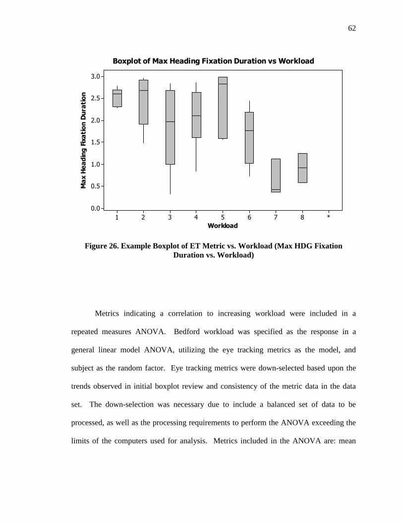
62
Workload
Max Heading Fixation Duration
*87654321
3.0
2.5
2.0
1.5
1.0
0.5
0.0
Boxplot of Max Heading Fixation Duration vs Workload
Figure 26. Example Boxplot of ET Metric vs. Workload (Max HDG Fixation Duration vs. Workload)
Metrics indicating a correlation to increasing workload were included in a
repeated measures ANOVA. Bedford workload was specified as the response in a
general linear model ANOVA, utilizing the eye tracking metrics as the model, and
subject as the random factor. Eye tracking metrics were down-selected based upon the
trends observed in initial boxplot review and consistency of the metric data in the data
set. The down-selection was necessary due to include a balanced set of data to be
processed, as well as the processing requirements to perform the ANOVA exceeding the
limits of the computers used for analysis. Metrics included in the ANOVA are: mean
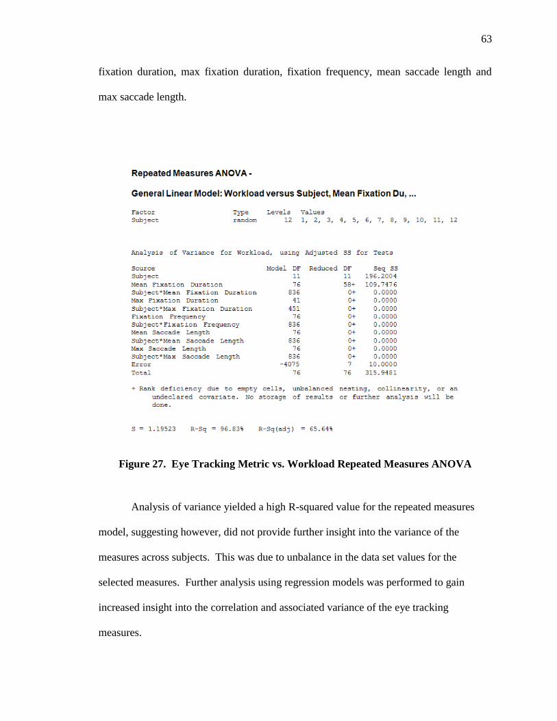
63
fixation duration, max fixation duration, fixation frequency, mean saccade length and
max saccade length.
Figure 27. Eye Tracking Metric vs. Workload Repeated Measures ANOVA
Analysis of variance yielded a high R-squared value for the repeated measures
model, suggesting however, did not provide further insight into the variance of the
measures across subjects. This was due to unbalance in the data set values for the
selected measures. Further analysis using regression models was performed to gain
increased insight into the correlation and associated variance of the eye tracking
measures.
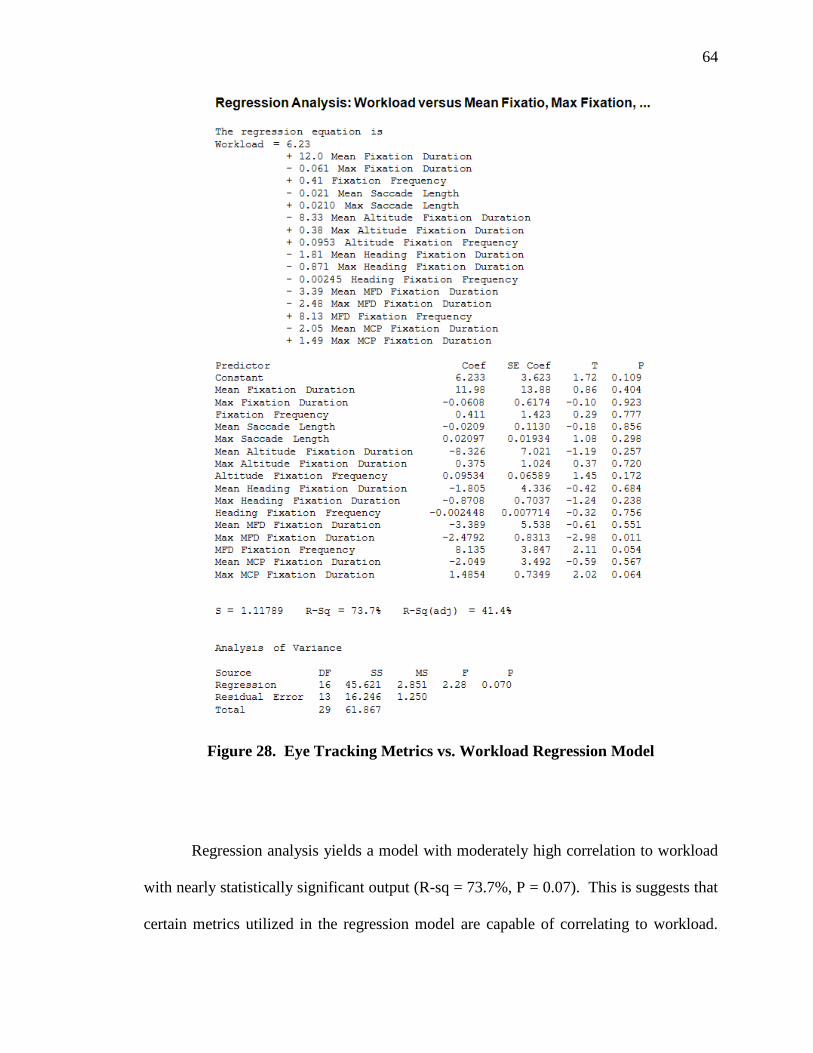
64
Figure 28. Eye Tracking Metrics vs. Workload Regression Model
Regression analysis yields a model with moderately high correlation to workload
with nearly statistically significant output (R-sq = 73.7%, P = 0.07). This is suggests that
certain metrics utilized in the regression model are capable of correlating to workload.
65
Some components were more statistically significant than others, particularly metrics
specific to regions of interest, such as the MFD fixation frequency (P=0.054) and Max
MCP fixation duration (P = 0.064). These metrics and metrics specific to a given region
of interest indicate a significantly higher level of significance to the overall regression
model. This provides insight suggesting that the workload on the pilot changes the pilots
eye movement behavior specific to a given instrument, likely dependent on the situation
inducing the workload, such as a specific task.
To determine the effect of task on workload, a repeated measures ANOVA was
performed to identify the variance of the task across pilots against workload. This was
performed in an effort to understand the connection to flight task and a given workload.
The flight tasks were defined previously as the independent variables condition and land
or go around. The condition was broken down into two binary sub categories; F/D on or
off and Autopilot on or off. This was done to more clearly specify what flight mode state
the aircraft was in for the specified test run.
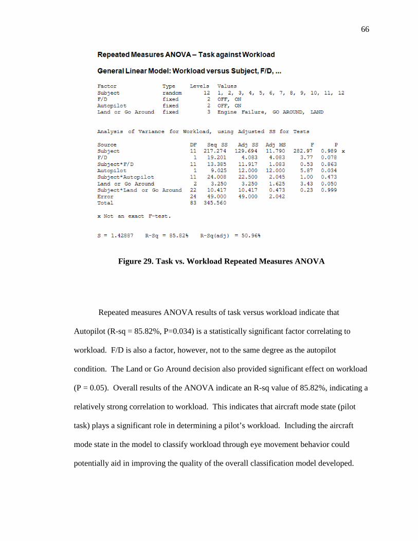
66
Figure 29. Task vs. Workload Repeated Measures ANOVA
Repeated measures ANOVA results of task versus workload indicate that
Autopilot (R-sq = 85.82%, P=0.034) is a statistically significant factor correlating to
workload. F/D is also a factor, however, not to the same degree as the autopilot
condition. The Land or Go Around decision also provided significant effect on workload
(P = 0.05). Overall results of the ANOVA indicate an R-sq value of 85.82%, indicating a
relatively strong correlation to workload. This indicates that aircraft mode state (pilot
task) plays a significant role in determining a pilot’s workload. Including the aircraft
mode state in the model to classify workload through eye movement behavior could
potentially aid in improving the quality of the overall classification model developed.
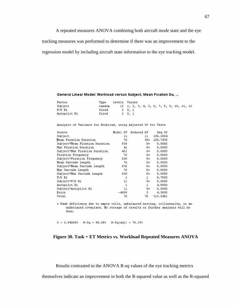
67
A repeated measures ANOVA combining both aircraft mode state and the eye
tracking measures was performed to determine if there was an improvement to the
regression model by including aircraft state information to the eye tracking model.
Figure 30. Task + ET Metrics vs. Workload Repeated Measures ANOVA
Results contrasted to the ANOVA R-sq values of the eye tracking metrics
themselves indicate an improvement in both the R-squared value as well as the R-squared

68
adjusted value. This suggests that the general linear model is improved by including the
aircraft mode state. However, due to unbalance in the data set values for each metric
included in the ANOVA, further variance analysis and statistical significance was not
established. Regression analysis on the eye tracking metrics used in the regression model
earlier (Figure 28. Eye Tracking Metrics vs. Workload Regression Model) was
performed again with the inclusion of the aircraft mode state.
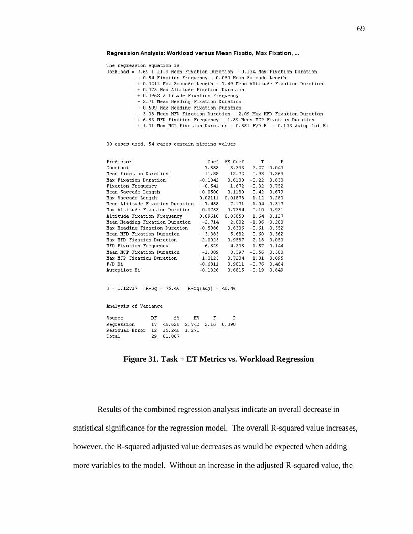
69
Figure 31. Task + ET Metrics vs. Workload Regression
Results of the combined regression analysis indicate an overall decrease in
statistical significance for the regression model. The overall R-squared value increases,
however, the R-squared adjusted value decreases as would be expected when adding
more variables to the model. Without an increase in the adjusted R-squared value, the
70
significance to adding the aircraft mode state is minimal to the model generated. F/D and
Autopilot state modes both indicate a P value greater than 0.46 providing no statistical
significance when combined with the metrics presently included in the model.
Results Conclusion
Development of a workload algorithm driven by eye tracking metrics is the
ultimate goal in aiding the initiative to classify operator state in real time flight deck
operations. Based upon this data set of pilot eye movements there is a wealth of
information that can continue to be mined for further insights into such eye movement
behaviors. Information taken from this analysis of the eye movement behavior trends
provides a significant starting point to develop a fully functional workload algorithm
based upon eye tracking metrics. Analysis of task and eye movement behaviors
individually indicate that each are associated to workload in some capacity, as is shown
in the repeated measures and regression analysis (Figure 27. Eye Tracking Metric vs.
Workload Repeated Measures ANOVA; Figure 29. Task vs. Workload Repeated
Measures ANOVA). Whether the two information sources can be combined to create an
increasingly effective model to classify workload is still uncertain. Several eye tracking
metrics indicated statistical significance or near statistical significance to the regression
model, all of which were eye movement behaviors specific to a given area of interest,
such as Max MFD Fixation Frequency (see Figure 28. Eye Tracking Metrics vs.
Workload Regression Model). To this extent, further research initiatives must be taken to
determine which combination of areas of interest metrics are the most useful in
classifying pilot workload.

71
CHAPTER 5.
CATS INTEGRATION
Cognitive Avionics Tool-Set (CATS)
The Cognitive Avionics Tool-Set (CATS) is a software application that provides a
graphical user interface to organizing sets of physiological data. Developed by Blaze
Keller of the Operator Performance Laboratory, it has been used in a beta version format
for several studies. The ultimate goal of CATS is to be able to compile several sources of
physiological data and generate analysis outputs of that data in a usable and presentable
form. Beyond this goal, taking all of the same physiological inputs (EEG, ECG,
respiration rate, body temp, eye tracking, etc.) real-time analysis will provide instant
feedback of pilot workload (Schnell, Keller, & Macuda, Application of the Cognitive
Avionics Tool Set (CATS) in Airborne Operator State Classification, 2007). CATS has
been utilized in a study done by the Operator Performance Laboratory in collaboration
with the National Research Council (NRC) of Canada. Initial intention of CATS is to be
used on avionics platforms as was done in a rotorcraft study in Ottawa, Ontario were
physiological measurements were fed into CATS and organized for data analysis
(Schnell, Keller, & Macuda, 2007). Other applications can utilize CATS as well due to
the underlying premise of CATS utility is to classify workload based upon physiological
measurement, such as pilot training effectiveness (Schnell, Keller, & Poolman, Quality of
training effectiveness assessment (QTEA); a Neurophsiologically based method to
enhance flight training, 2008). The underlying research which drives the classification
model however, is specific to flight deck operations.
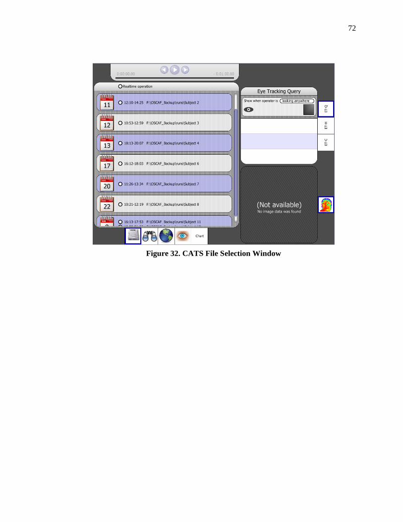
72
Figure 32. CATS File Selection Window
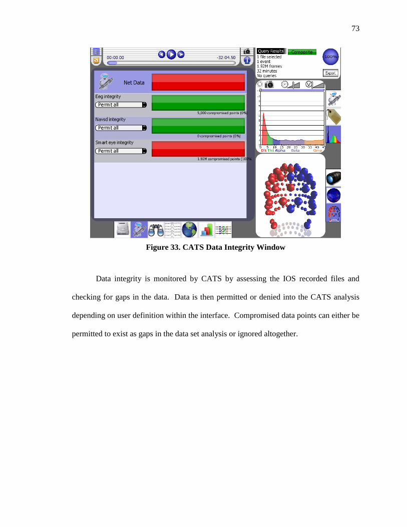
73
Figure 33. CATS Data Integrity Window
Data integrity is monitored by CATS by assessing the IOS recorded files and
checking for gaps in the data. Data is then permitted or denied into the CATS analysis
depending on user definition within the interface. Compromised data points can either be
permitted to exist as gaps in the data set analysis or ignored altogether.
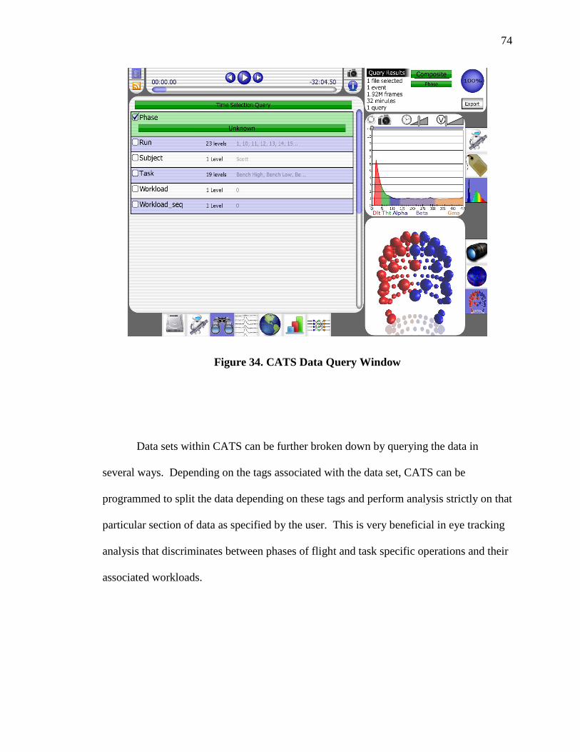
74
Figure 34. CATS Data Query Window
Data sets within CATS can be further broken down by querying the data in
several ways. Depending on the tags associated with the data set, CATS can be
programmed to split the data depending on these tags and perform analysis strictly on that
particular section of data as specified by the user. This is very beneficial in eye tracking
analysis that discriminates between phases of flight and task specific operations and their
associated workloads.
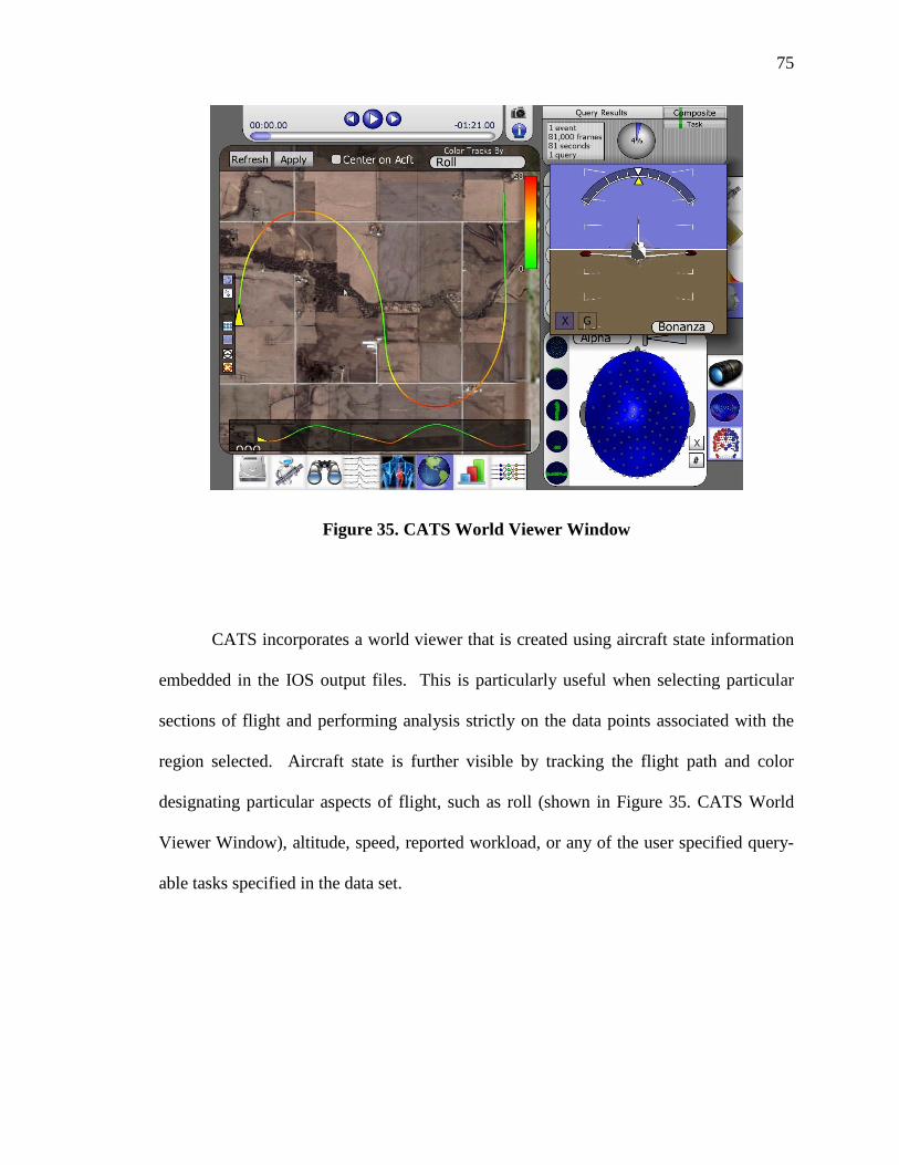
75
Figure 35. CATS World Viewer Window
CATS incorporates a world viewer that is created using aircraft state information
embedded in the IOS output files. This is particularly useful when selecting particular
sections of flight and performing analysis strictly on the data points associated with the
region selected. Aircraft state is further visible by tracking the flight path and color
designating particular aspects of flight, such as roll (shown in Figure 35. CATS World
Viewer Window), altitude, speed, reported workload, or any of the user specified query-
able tasks specified in the data set.
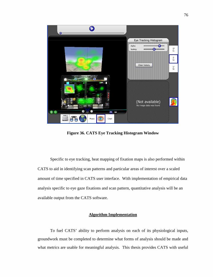
76
Figure 36. CATS Eye Tracking Histogram Window
Specific to eye tracking, heat mapping of fixation maps is also performed within
CATS to aid in identifying scan patterns and particular areas of interest over a scaled
amount of time specified in CATS user interface. With implementation of empirical data
analysis specific to eye gaze fixations and scan pattern, quantitative analysis will be an
available output from the CATS software.
Algorithm Implementation
To fuel CATS’ ability to perform analysis on each of its physiological inputs,
groundwork must be completed to determine what forms of analysis should be made and
what metrics are usable for meaningful analysis. This thesis provides CATS with useful
77
information pertaining to the eye tracking facet of CATS’ physiological analysis suite.
Acquisition and analysis of empirical data creates algorithms for each metric, and
ultimately one metric to assess workload based upon the pertinent eye tracking metrics.
Real-Time Workload Estimation
CATS currently utilizes neural analysis, eye tracking, heart rate (ECG), and flight
performance as general metrics that feed an overall workload estimation of the subject
being analyzed. Development of regression models in eye tracking is utilized in CATS
from this research, derived from empirical data collected in this study. For real time
assessment of the pilots’ fixation behavior, the average duration of fixations can be
calculated for a window of 15 seconds, which typically includes a series of 10 to 20
fixations sufficient enough to provide a statistically significant average. The real time
fixation behavior variables are then assessed based upon empirical analysis following the
results of this research initiative with coefficients dependent on relativity to the
normalization of these behaviors.
Utility of Algorithm for Real-Time Classification
The regression models developed based upon the composite results of this study is
statistically significant and can be utilized as a classifier algorithm to be validated in real-
time assessment tests in future studies. See Error! Reference source not found.Figure
26. Subject 2 Waypoint Regression Analysis, Error! Reference source not
found.Figure 27. Subject 7 Waypoint Regression Analysis and Error! Reference
source not found.Figure 31. Fixation Frequency Composite Regression. The
78
coefficients relating each metric analyzed are the important components to generating a
general real-time classification algorithm.
For analysis of real-time classification, it is recommended to use a window of
time to perform general statistics of the various metrics that make sense. Average
fixation duration was calculated over a moving time frame of 15 seconds to be able to
capture enough fixations to produce a significant average of the metric. Entropy was
calculated with a moving time frame of 30 seconds, since it is a metric assessing the
variability that exists in a scan pattern or the spread of fixations. Shorter time frames for
this metric will not provide enough time for a pattern to be recognizable, yielding no
significance to the standard deviation values, but too long of a time frame will not be
capable of observing the short term changes in fixations that occur in flight deck
operations.
Industry Utilization of Operator State Classification Information
There are several applications that are capable of utilizing real-time operator state
classification. Training of pilots can be enhanced by importing knowledge of the
student’s workload, allowing the instructor to increase or decrease the pace of the training
to maximize the efficiency of the training for the student based upon their cognitive
capacity. Allowing the avionics of flight decks to be aware of the pilot’s cognitive state
provides an entirely new avenue for avionics to follow; adaptive automation systems,
enhanced visual ergonomics that adapt to rare situations such as unusual attitude, pilot
attention retention systems, sleep mitigation systems, etc.

79
CHAPTER 6.
FUTURE RESEARCH
Further Initiatives to Be Pursued
Analysis of potentially useful metrics, such as eye blinks should be pursued. Eye
blinks were not analyzed due to eye tracker outputs not transmitting the correct data to be
recorded in the data set. Unfortunately this was unrecoverable for any of the subjects in
this study, and it still holds strict interest due to eye blink as a metric being a very rich
source of operator state information in previous studies.
Continued research of the present data set could be pursued to further the
interaction effects of the various areas of interest. Further preprocessing of the data must
be completed to fully fill the data set so balanced ANOVAs can be performed to gain full
insight of variance across subjects for all eye tracking metrics. A stepwise regression
would also be beneficial in determining which metrics yield the greatest impact on the
regression model against workload. Validation of the data set regression models should
also be completed to determine the overall effectiveness of a developed model based
upon this data set.
A similar study could be performed with a new method to induce workload and
collect the subjective baseline results at a higher resolution than was done with the
Bedford workload ratings collected in this study (1 data point / 2 min). A possible
approach would include shorter test runs with a precisely induced workload enforced

80
upon the pilot. A post run subjective response would be sufficient to produce a subjective
baseline to regress against. This is necessary to attain increasingly accurate real-time
analysis algorithms for any physiological response system such as an eye tracker. A
bottom up approach study could be done that induces workload in a situation by situation
manner that requires pilots to react and that reaction could tag a set of data and their
associative metrics. Bottom line requires a closing of the gap between data collection
rates and subjective workload response rates to limit the error brought about by
regression interpolation of real-time metrics.
This study provides a simple insight into the trends of eye movement metrics as
they respond to induced workload in a cockpit performing an approach task. Further
studies to determine which metrics are useful in classifying workload during specific
tasks and which metrics classify workload generically can still be completed. Further
research initiatives can also be done to assess the connection between standard eye
movement behaviors in a flight deck as they pertain to individual tasks versus workload.
It is believed that certain tasks performed on the flight deck induce specific eye
movement behaviors. If this is the case, it is theoretically possible to assume that
changes in expected eye tracking behavior may occur depending on the flight task, such
as cruising and performing an approach.
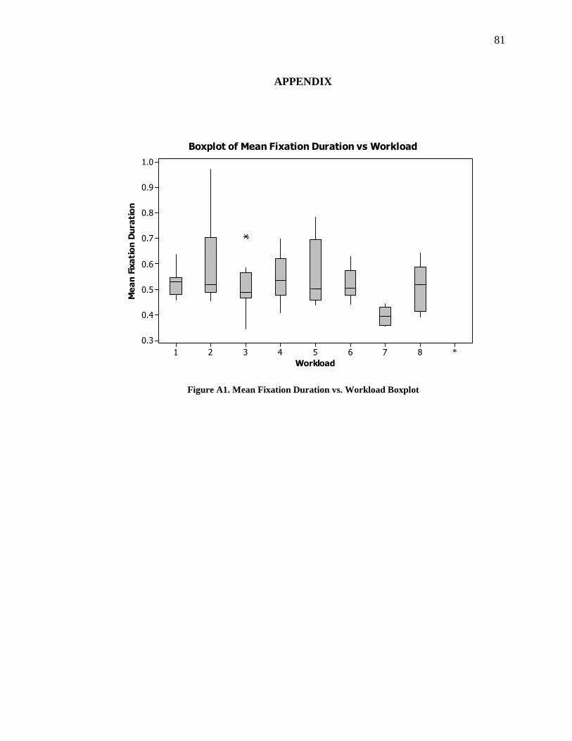
81
APPENDIX
Workload
Mean Fixation Duration
*87654321
1.0
0.9
0.8
0.7
0.6
0.5
0.4
0.3
Boxplot of Mean Fixation Duration vs Workload
Figure A1. Mean Fixation Duration vs. Workload Boxplot
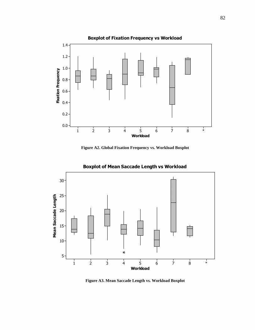
82
Workload
Fixation Frequency
*87654321
1.4
1.2
1.0
0.8
0.6
0.4
0.2
0.0
Boxplot of Fixation Frequency vs Workload
Figure A2. Global Fixation Frequency vs. Workload Boxplot
Workload
Mean Saccade Length
*87654321
30
25
20
15
10
5
Boxplot of Mean Saccade Length vs Workload
Figure A3. Mean Saccade Length vs. Workload Boxplot
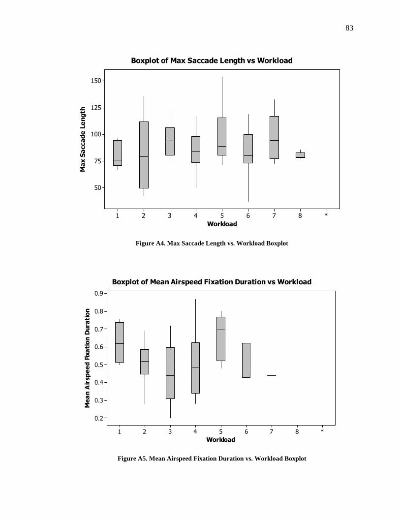
83
Workload
Max Saccade Length
*87654321
150
125
100
75
50
Boxplot of Max Saccade Length vs Workload
Figure A4. Max Saccade Length vs. Workload Boxplot
Workload
Mean Airspeed Fixation Duration
*87654321
0.9
0.8
0.7
0.6
0.5
0.4
0.3
0.2
Boxplot of Mean Airspeed Fixation Duration vs Workload
Figure A5. Mean Airspeed Fixation Duration vs. Workload Boxplot
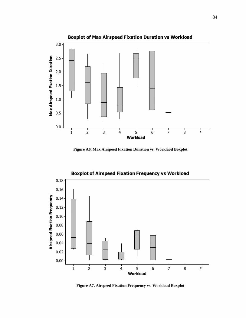
84
Workload
Max Airspeed Fixation Duration
*87654321
3.0
2.5
2.0
1.5
1.0
0.5
0.0
Boxplot of Max Airspeed Fixation Duration vs Workload
Figure A6. Max Airspeed Fixation Duration vs. Worklaod Boxplot
Workload
Airspeed Fixation Frequency
*87654321
0.18
0.16
0.14
0.12
0.10
0.08
0.06
0.04
0.02
0.00
Boxplot of Airspeed Fixation Frequency vs Workload
Figure A7. Airspeed Fixation Frequency vs. Workload Boxplot
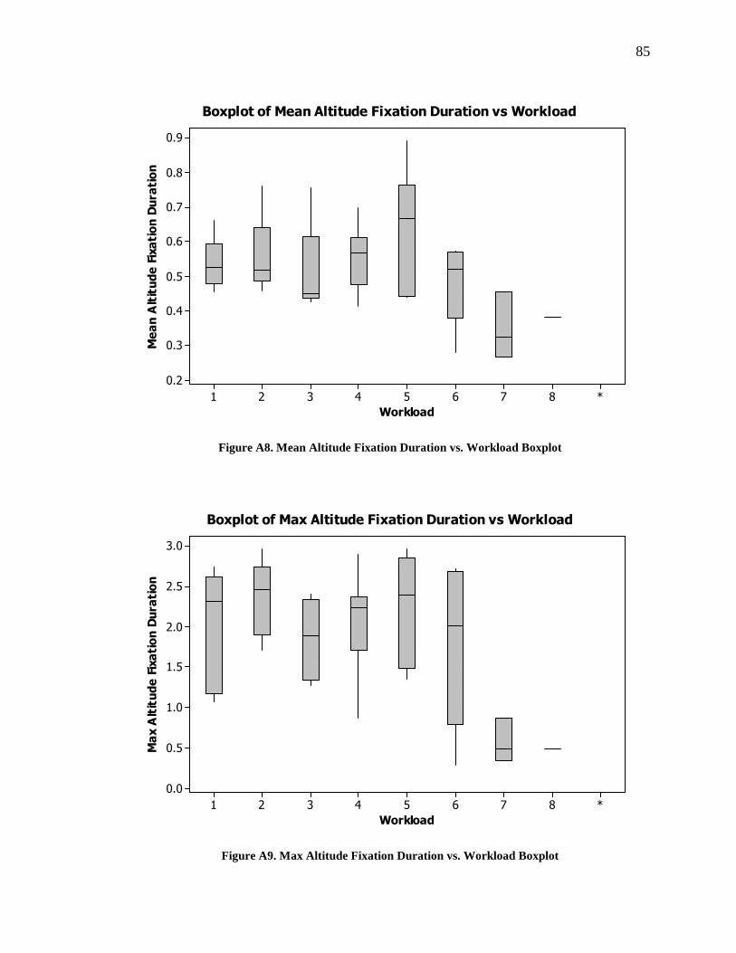
85
Workload
Mean Altitude Fixation Duration
*87654321
0.9
0.8
0.7
0.6
0.5
0.4
0.3
0.2
Boxplot of Mean Altitude Fixation Duration vs Workload
Figure A8. Mean Altitude Fixation Duration vs. Workload Boxplot
Workload
Max Altitude Fixation Duration
*87654321
3.0
2.5
2.0
1.5
1.0
0.5
0.0
Boxplot of Max Altitude Fixation Duration vs Workload
Figure A9. Max Altitude Fixation Duration vs. Workload Boxplot
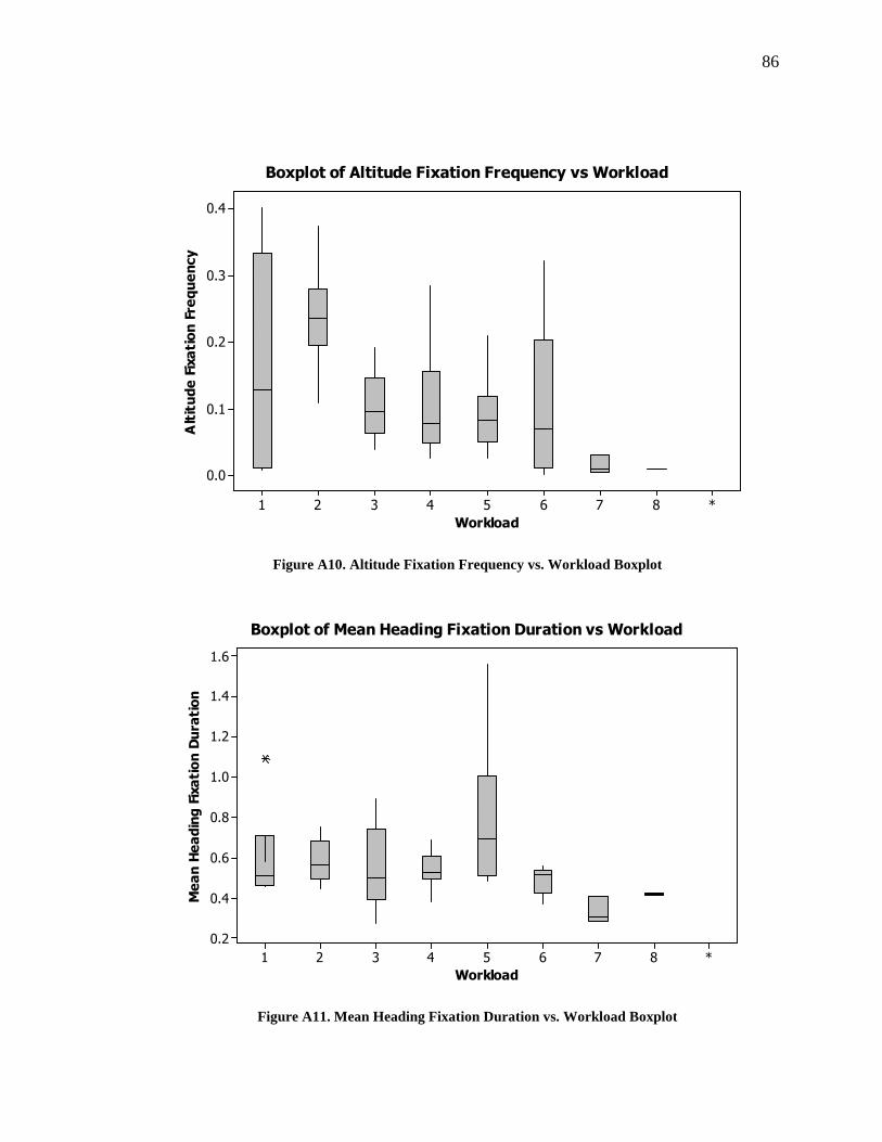
86
Workload
Altitude Fixation Frequency
*87654321
0.4
0.3
0.2
0.1
0.0
Boxplot of Altitude Fixation Frequency vs Workload
Figure A10. Altitude Fixation Frequency vs. Workload Boxplot
Workload
Mean Heading Fixation Duration
*87654321
1.6
1.4
1.2
1.0
0.8
0.6
0.4
0.2
Boxplot of Mean Heading Fixation Duration vs Workload
Figure A11. Mean Heading Fixation Duration vs. Workload Boxplot
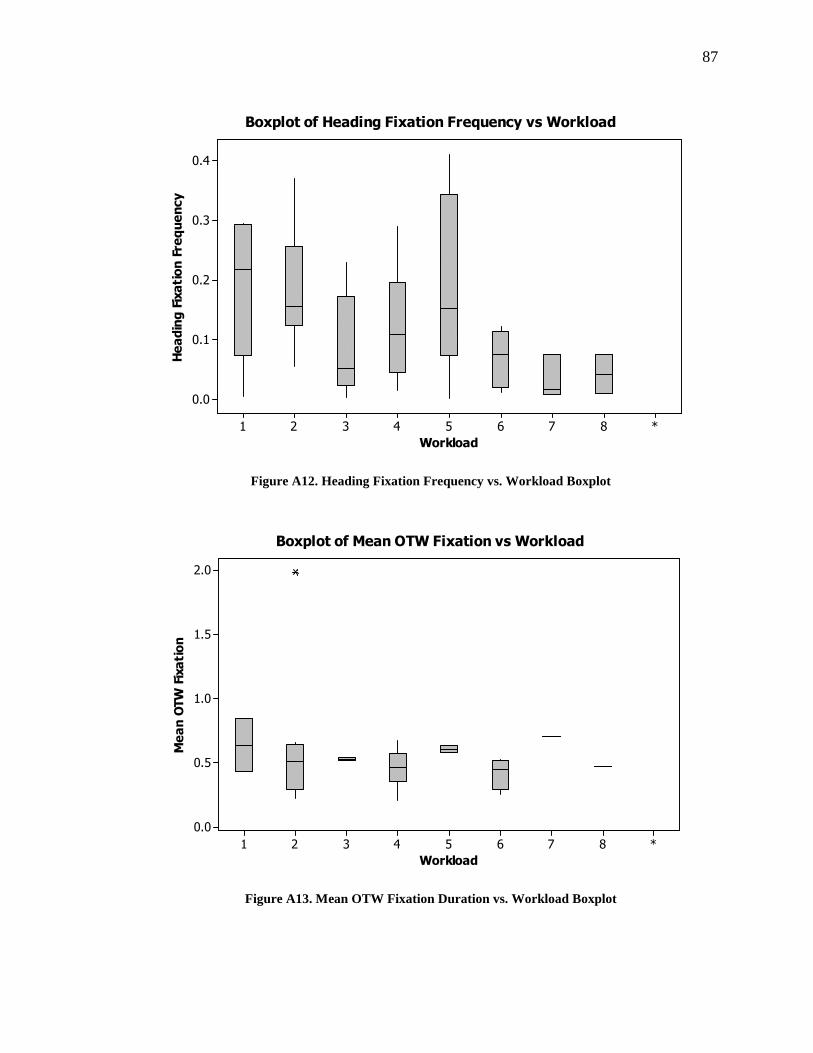
87
Workload
Heading Fixation Frequency
*87654321
0.4
0.3
0.2
0.1
0.0
Boxplot of Heading Fixation Frequency vs Workload
Figure A12. Heading Fixation Frequency vs. Workload Boxplot
Workload
Mean OTW Fixation
*87654321
2.0
1.5
1.0
0.5
0.0
Boxplot of Mean OTW Fixation vs Workload
Figure A13. Mean OTW Fixation Duration vs. Workload Boxplot
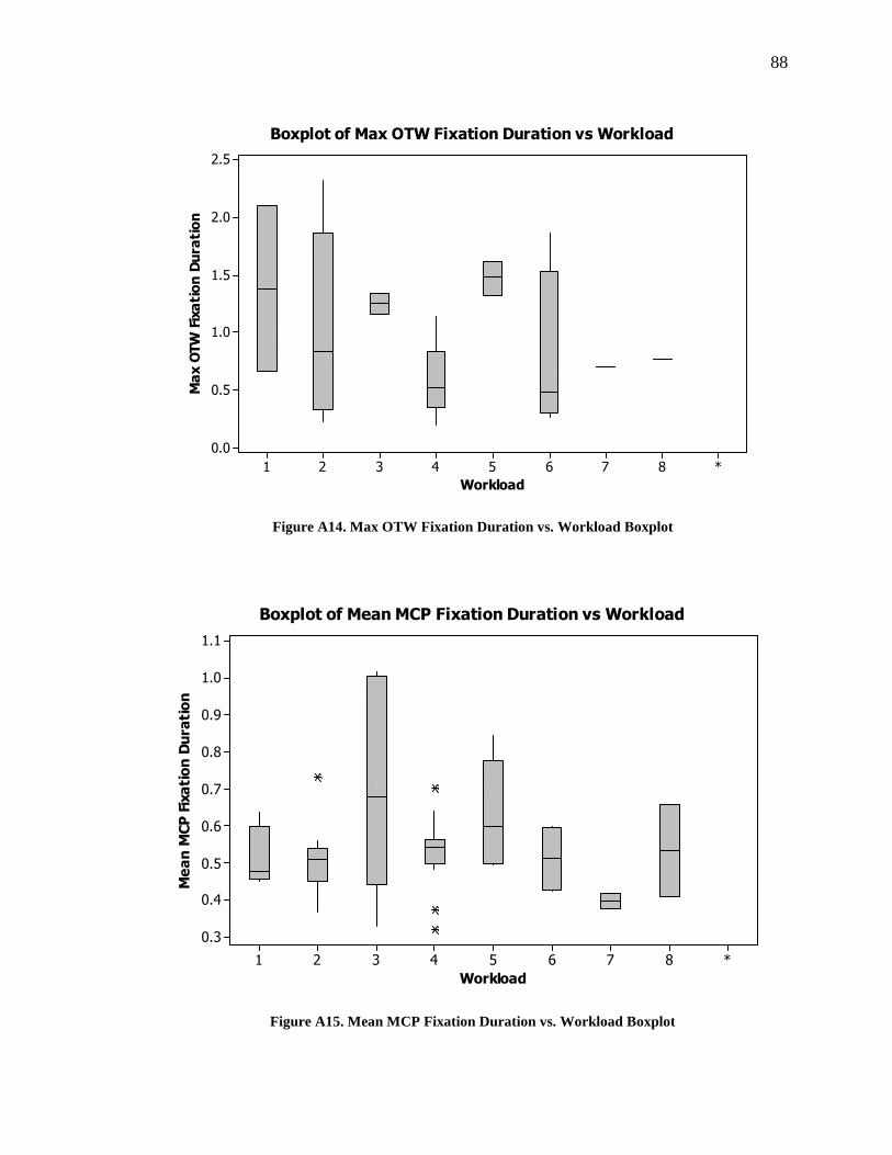
88
Workload
Max OTW Fixation Duration
*87654321
2.5
2.0
1.5
1.0
0.5
0.0
Boxplot of Max OTW Fixation Duration vs Workload
Figure A14. Max OTW Fixation Duration vs. Workload Boxplot
Workload
Mean M
CP Fixation Duration
*87654321
1.1
1.0
0.9
0.8
0.7
0.6
0.5
0.4
0.3
Boxplot of Mean MCP Fixation Duration vs Workload
Figure A15. Mean MCP Fixation Duration vs. Workload Boxplot
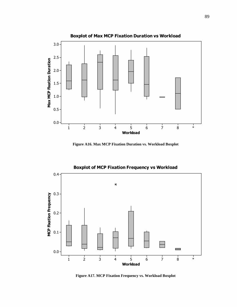
89
Workload
Max M
CP Fixation Duration
*87654321
3.0
2.5
2.0
1.5
1.0
0.5
0.0
Boxplot of Max MCP Fixation Duration vs Workload
Figure A16. Max MCP Fixation Duration vs. Workload Boxplot
Workload
MCP Fixation Frequency
*87654321
0.4
0.3
0.2
0.1
0.0
Boxplot of MCP Fixation Frequency vs Workload
Figure A17. MCP Fixation Frequency vs. Workload Boxplot
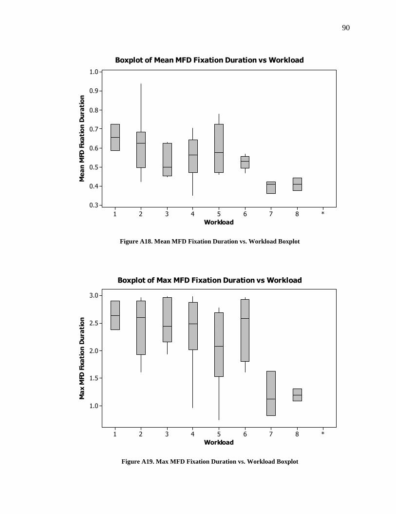
90
Workload
Mean M
FD Fixation Duration
*87654321
1.0
0.9
0.8
0.7
0.6
0.5
0.4
0.3
Boxplot of Mean MFD Fixation Duration vs Workload
Figure A18. Mean MFD Fixation Duration vs. Workload Boxplot
Workload
Max M
FD Fixation Duration
*87654321
3.0
2.5
2.0
1.5
1.0
Boxplot of Max MFD Fixation Duration vs Workload
Figure A19. Max MFD Fixation Duration vs. Workload Boxplot
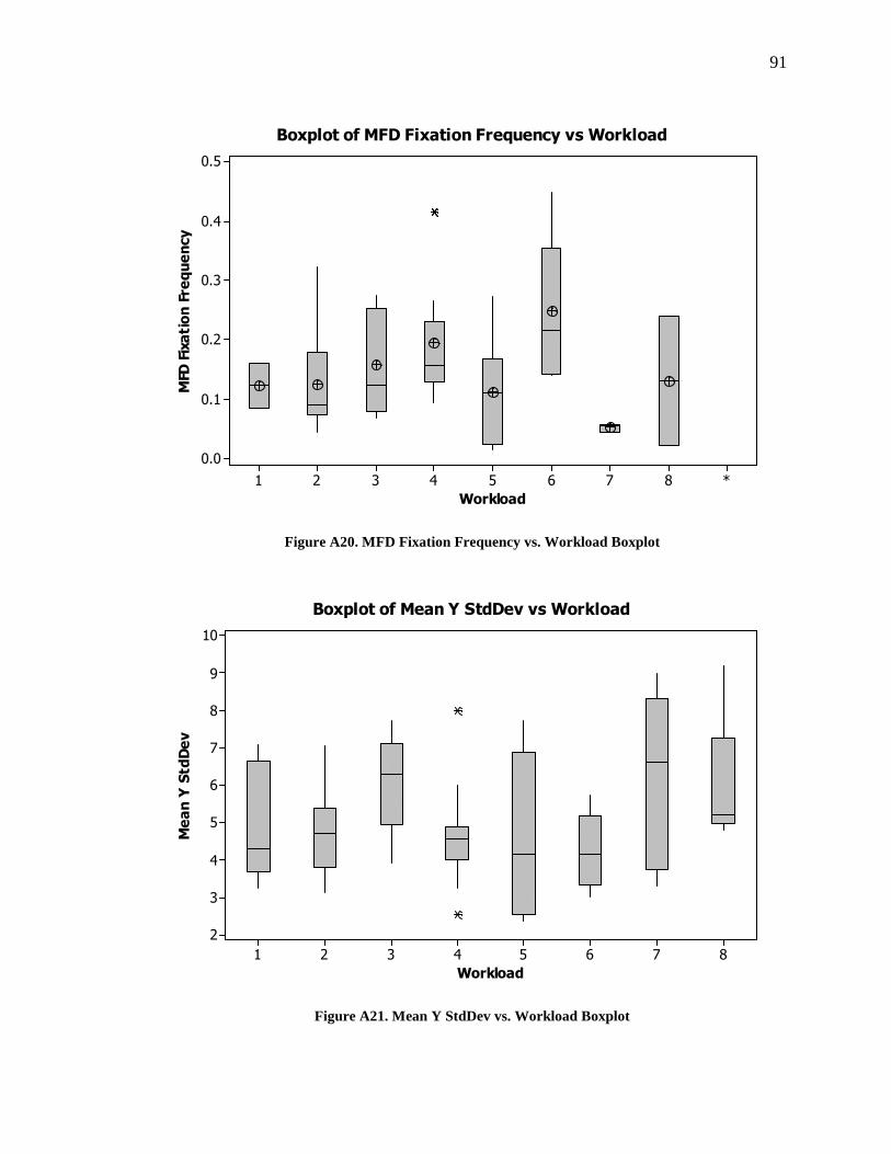
91
Workload
MFD Fixation Frequency
*87654321
0.5
0.4
0.3
0.2
0.1
0.0
Boxplot of MFD Fixation Frequency vs Workload
Figure A20. MFD Fixation Frequency vs. Workload Boxplot
Workload
Mean Y StdDev
87654321
10
9
8
7
6
5
4
3
2
Boxplot of Mean Y StdDev vs Workload
Figure A21. Mean Y StdDev vs. Workload Boxplot
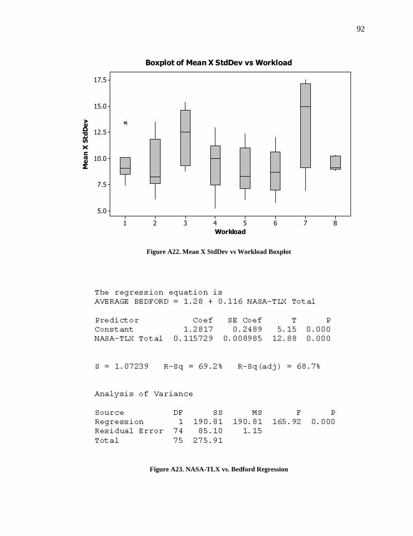
92
Workload
Mean X StdDev
87654321
17.5
15.0
12.5
10.0
7.5
5.0
Boxplot of Mean X StdDev vs Workload
Figure A22. Mean X StdDev vs Workload Boxplot
Figure A23. NASA-TLX vs. Bedford Regression
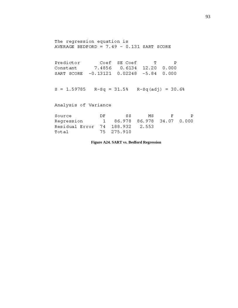
93
Figure A24. SART vs. Bedford Regression
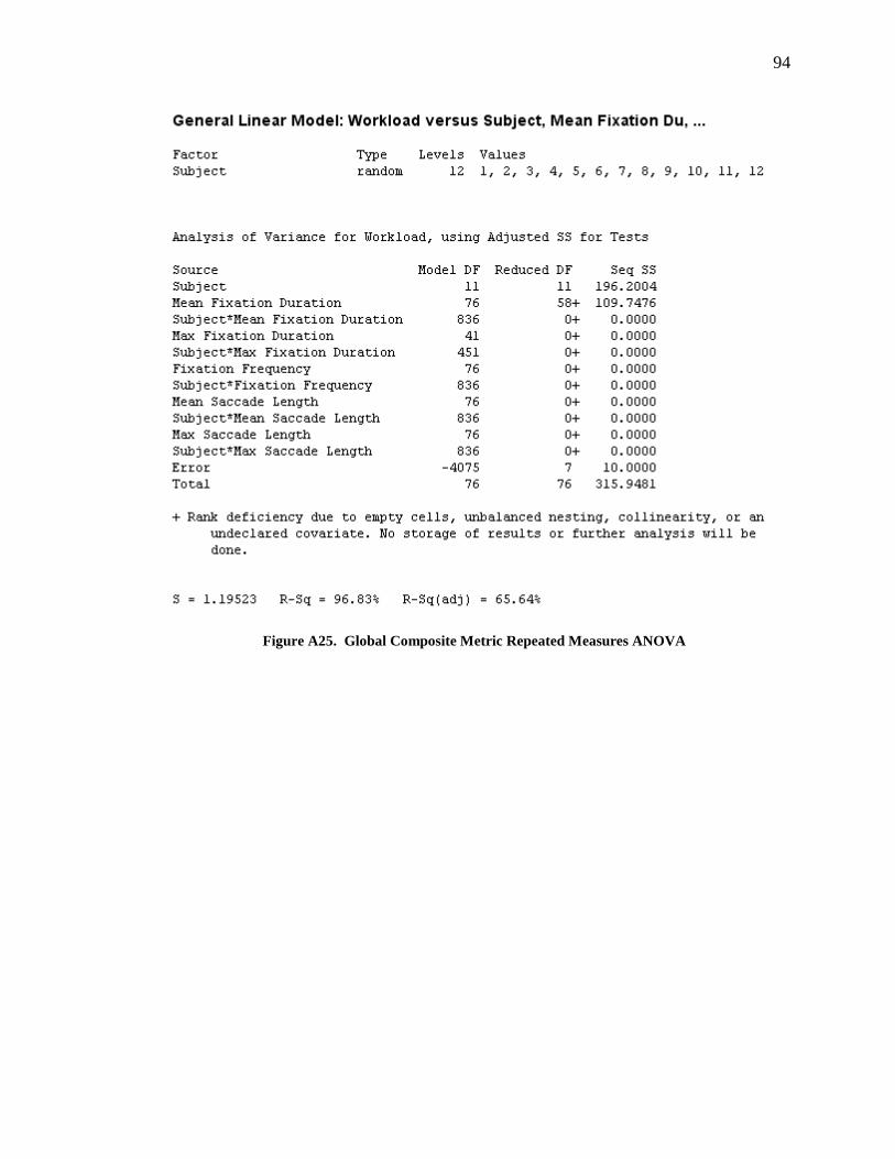
94
Figure A25. Global Composite Metric Repeated Measures ANOVA
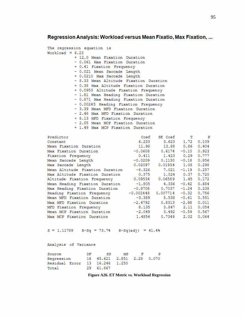
95
Figure A26. ET Metric vs. Workload Regression
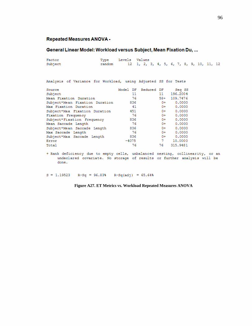
96
Figure A27. ET Metrics vs. Workload Repeated Measures ANOVA
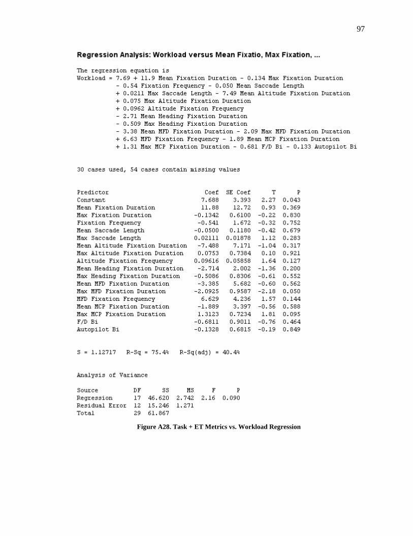
97
Figure A28. Task + ET Metrics vs. Workload Regression
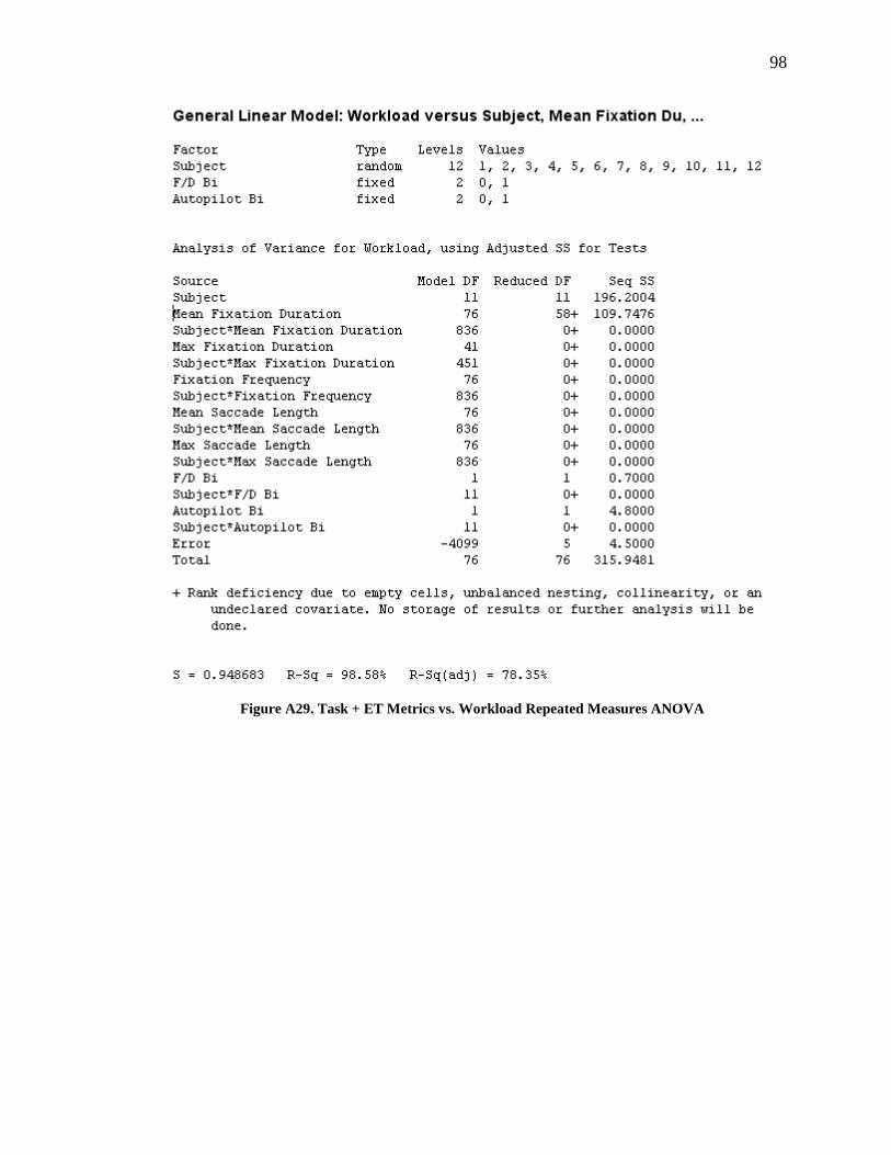
98
Figure A29. Task + ET Metrics vs. Workload Repeated Measures ANOVA
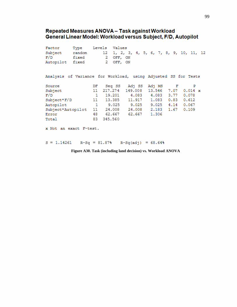
99
Figure A30. Task (including land decision) vs. Workload ANOVA
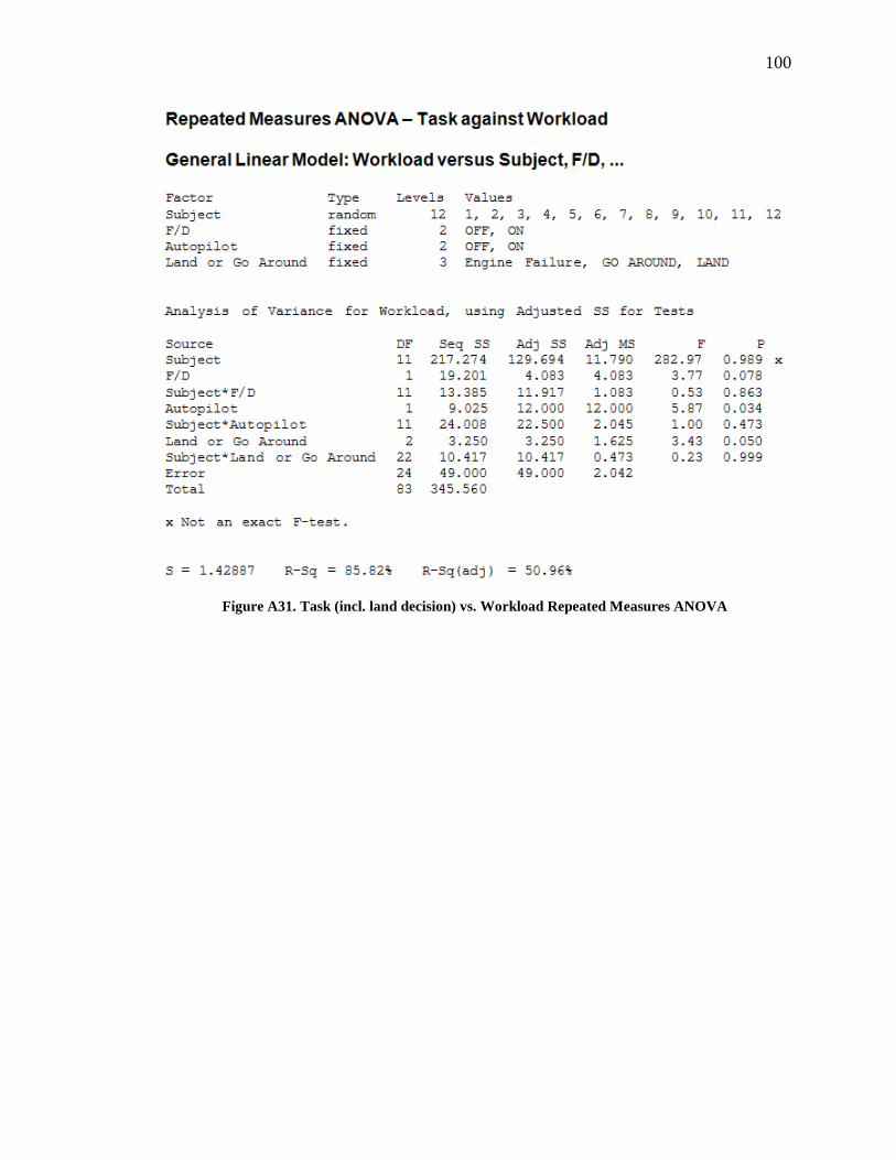
100
Figure A31. Task (incl. land decision) vs. Workload Repeated Measures ANOVA

101
BIBLIOGRAPHY Altonen, A., Hyrskykari, A., & Raiha, K. (1998). 101 Spots, or how do users read menus? Proceedings of CHI 98 Human Factors in Computing Systems (pp. 132-139). ACM Press. Applied Science Laboratories. (2007). Eyenal (Eye-Analysis) Software Manual, Windows application Version 2.96, Manual Version 1.41. Applied Science Laboratories. Backs, R., & Walrath, L. (1992). Eye movement and pupillary response indices of mental workload during visual search of symbolic displays. Applied Ergonomics , 243-254. Boyce, C., Ross, A., Monaco, M., Hornak, L., & Xin, L. (2006). Multispectral Iris Analysis: A Preliminary Study. Computer Vision and Pattern Recognition Workshop on Biometrics, (p. 51). New York. Brookings, J. B., Wilson, G. F., & Swain, C. R. (1996). Psychophysiological responses to changes in workload during simulated air traffic control. Dayton, OH: Biological Psychology. Callan, D. (1998). Eye movement relationships to excessive performance error in aviation. Proceedings of the Human Factors and Ergonomics Society 42nd Annual Meeting (pp. 1132-1136). Santa Moica, CA: Human Factors and Ergonomics Society. Card, S. (1984). Visual Search of computer command menus. In H. Bouma, & D. Bouwhuis, Attention and Performance X, Control of Language Processes. Hillsdale, NJ: Lawrence Erlbaum Associates. Crosby, M., & Peterson, W. (1991). Using eye movements to clasify search strategies. Proceedings of the Human Factors Society 35th Annual Meeting (pp. 1476-1480). Santa Monica: Human Factors and Ergonomics Society. Di Nocera, F., Terenzi, M., & Camilli, M. (2006). Another look at scanpath: distance to nearest neighbor as a measure of mental workload. In D. de Waard, K. Brookhuis, & A. Toffetti, Developments in Human Factors in Transportation, Design, and Evaluation (pp. 1-9). Maastricht, the Netherlands: Shaker Publishing. Fitts, P. M., Jones, R. E., & Milton, J. L. (1950). Eye movements of aircraft pilots during instrument-landing approaches. Aeronautical Engineering Review , 24-29. Gilland, J. (2008). Driving, Eye Tracking and Visual Entropy: Exploration of Age and Task Effects. University of South Dakota.

102
Goldberg, J., & Kotval, X. (1998). Eye movement-based evaluation of the computer interface. In S. Kumar, Advances in Ocupational Ergonomics and Safety (pp. 529-532). Amsterdam: ISO Press. Granholm, E., Asarnow, R. F., Sarkin, A. J., & Dykes, K. L. (1996). Pupillary responses index cognitive resource limitations. Psychophysiology , 457-461. Hankins, T., & Wilson, G. (1998). A comparison of heart rate, eye activity, EEG and subjective measures of pilot mental workload during flight. Aviation, space and Environmental Medicine , 360-367. Harris, R. L., Glover, B. J., & Spady, A. A. (1986). Analytical Techniques of Pilot Scanning Behavior and Their Application. Hampton, VA: NASA Technical Paper 2525. Hendrickson, J. (1989). Performance, preference, and visual scan patterns on a menu-based system: implications for interface design. Proceedings of the ACM CHI '89 Human Factors in Computing Systems Conference (pp. 217-222). ACM Press. Hilburn, B. (2004). Measuring head-down time via area-of interest analysis: operational and experimental data. In D. De Waard, K. Brookhui, R. Van Egmond, & T. Boersma, Human Factors in Design, Safety, and Management (pp. 427-436). Maastricht, the Netherlands: Shaker Publishing. Itoh, Y., Hayashi, Y., Tsukui, I., & Saito, S. (1990). The ergonomic evaluation of eye movements and mental workload in aircraft pilots. Ergonomics , 719-733. Jacob, R. J., & Karn, K. S. (2003). Eye tracking in human-computer interaction and usability research: Ready to deliver the promises. The Mind's eye: Cognitive The Mind's Eye: Cognitive and Applied Aspects of Eye Movement Research , 573 - 603. Just, M. A., & Carpenter, P. A. (1993). The Intensity Dimension of Thought: Pupillometric Indices of Sentence Processing. Canadian journal of Experimental Psychology , 310-339. Kotval, X., & Goldberg, J. (1998). Eye movements and interface components grouping: an evaluation method. Proceedings of the 42nd Annual Meeting of the Human Factors and Ergonomics Society (pp. 486-490). Santa Monica: Human Factors and Ergonomics Society. Nave, R. (2000, June). The Retina of the Human Eye. Retrieved June 2009, from GSU Hyperphysics Webpage: http://hyperphysics.phy-astr.gsu.edu/Hbase/vision/retina.html Noton, D., & Stark, L. (1971). Eye movements and visual perception (Eye movements and visual perception, describing scan path for memory traces). Scientific American , 35-43.

103
Rao, R. P., Zelinsky, G. J., Hayhoe, M. M., & Ballard, D. H. (1997). Eye Movements in Visual Cognition A Computational Study. National Resource Laboratory for the Study of Brain Behavior, University of rochester. Rayner, K., & Bertera, J. H. (1979). Reading without a Fovea. In Science (pp. 468-469). American Association for the Advancement of Society. Schnell, T., Keller, M., & Macuda, T. (2007). Application of the Cognitive Avionics Tool Set (CATS) in Airborne Operator State Classification. Augmented Cognition International Conference. Baltimore, MD: ACI. Schnell, T., Keller, M., & Macuda, T. (2007). Pilot State Classification and Mitigation in a Fixed and Rotary Wing Platform. Aerospace Medical Association annual conference (p. 377). New Orleans, LA: Aviation Space and Environmental Medicine. Schnell, T., Keller, M., & Poolman, P. (2008). Quality of training effectiveness assessment (QTEA); a Neurophsiologically based method to enhance flight training. Proceedings of the 27th Digital Avionics Systems Conference (DASC). St. Paul, MN: DASC. Simon, P., Rousseau, F., & Angue, J.-C. (1993). Quantitative Analysis of Mental Workload Influence on Eye Scanning Movements. Le Touquet, France: Systems, Man and Cybernetics. Van Orden, K. F., Limbert, W., Makeig, S., & Jung, T. -P. (2001). Eye Activity Correlates of Workload during a Visuospatial Memory Task. Human Factors , 111-121. Wang, H., Lin, S., Liu, X., & Kang, S. B. (2005). Separating Reflections in Human Iris Images for Illumination Estimation. Tenth IEEE International Conference on Computer Vision, (pp. 1691-1698). Beijing, China. Wilson, G. F., Purvis, B., Skelly, J., Fullenkamp, P., & Davis, I. (1987). Physiological data used to measure pilot workload in actual flight and simulator conditions. Proceedings from the 31st Annual Meeting of the Human Factors Socitey (pp. 779-783). New York: Human Factors Society. Wooding, D. S. (2002). Fixation Maps: Quantifying Eye-Movement Traces. New Orleans: ETRA. Yamamoto, S., & Kuto, Y. (1992). A method of evaluating VDT Scren layout by eye movement analysis. Ergonomics , 591-606. Yarbus, A. (1967). Eye Movements and Vision. Plenum Press.