Embed Size (px)
Citation preview

Technische Universität Dresden
Extraction and Detection of Fetal Electrocardiogramsfrom Abdominal Recordings
Fernando Andreotti Lage
von der Fakultät Elektrotechnik und Informationstechnik der Technische UniversitätDresden
zur Erlangung des akademischen Grades
Doktoringenieur
(Dr.-Ing.)
genehmigte Dissertation
Vorsitzender: Prof. Dr. rer. nat. Edmund Koch
Gutachter: Prof. Dr.-Ing. habil. Hagen Malberg
Prof. Dr. Maarten De Vos Tag der Einreichung: 07.11.2016
Prof. Dr. phil. nat. habil. Ronald Tetzlaff Tag der Verteidigung: 20.01.2017


Fernando Andreotti Lage(2017) - This work is licensed under the Creative Commons 4.0 License.

Abstract
The non-invasive fetal ECG (NIFECG), derived from abdominal surface electrodes, offers
novel diagnostic possibilities for prenatal medicine. Despite its straightforward applicability,
NIFECG signals are usually corrupted by many interfering sources. Most significantly, by the
maternal ECG (MECG), whose amplitude usually exceeds that of the fetal ECG (FECG) by
multiple times. The presence of additional noise sources (e.g. muscular/uterine noise, electrode
motion, etc.) further affects the signal-to-noise ratio (SNR) of the FECG. These interfering
sources, which typically show a strong non-stationary behavior, render the FECG extraction
and fetal QRS (FQRS) detection demanding signal processing tasks.
In this thesis, several of the challenges regarding NIFECG signal analysis were addressed.
In order to improve NIFECG extraction, the dynamic model of a Kalman filter approach was
extended, thus, providing a more adequate representation of the mixture of FECG, MECG, and
noise. In addition, aiming at the FECG signal quality assessment, novel metrics were proposed
and evaluated. Further, these quality metrics were applied in improving FQRS detection and
fetal heart rate estimation based on an innovative evolutionary algorithm and Kalman filtering
signal fusion, respectively. The elaborated methods were characterized in depth using both
simulated and clinical data, produced throughout this thesis. To stress-test extraction algorithms
under ideal circumstances, a comprehensive benchmark protocol was created and contributed
to an extensively improved NIFECG simulation toolbox. The developed toolbox and a large
simulated dataset were released under an open-source license, allowing researchers to compare
results in a reproducible manner. Furthermore, to validate the developed approaches under
more realistic and challenging situations, a clinical trial was performed in collaboration with
the University Hospital of Leipzig. Aside from serving as a test set for the developed algorithms,
the clinical trial enabled an exploratory research. This enables a better understanding about the
pathophysiological variables and measurement setup configurations that lead to changes in the
abdominal signal’s SNR. With such broad scope, this dissertation addresses many of the current
aspects of NIFECG analysis and provides future suggestions to establish NIFECG in clinical
settings.
i


Acknowledgments
First, I would like to thank Dr. Sebastian Zaunseder and Prof. Hagen Malberg for the
opportunity to be part of the IBMT as well as their supervision and support throughout the
process. I’d also like to thank the good men at the IBMT: Alex, Daniel, Felix, Johann and Martin,
for making the doctoral experience bearable with our fruitful Fridays 4 p.m. meetings. Likewise,
my appreciation to the several friends I made in Dresden, who made this time unforgettable.
I’d also like to thank our clinical partners from the University Hospital of Leipzig Dr. Alexan-
der Jank, Dr. Claudia Schmieder, Sophia Schröder, Susanne Fritze and Prof. Stepan Holger for
their helpful insights on the medical aspects of gestation, collecting data, and proving very
useful annotations. Also thanks to our colleagues at the Humboldt University of Berlin Dr. Maik
Riedl and Dr. Niels Wessel.
Many thanks to Prof. Gari Clifford and Prof. David Clifton for receiving me at the IBME -
Oxford. To the several collaborators and friends I made in England, particularly Joachim, Julien,
Alistair, Lisa and Tingting, for taking me in and providing me with a greatly productive time in
and out of pubs.
This work was sponsored by the Conselho Nacional de Desenvolvimento Tecnologico (CNPq -
Brazil) with a doctoral scholarship and by the TU Dresden Graduate Academy as part of the
Excellence Initiative of the German Federal and State Governments in the scope of travel and
completion grants. Without their financial support, this work would not have been possible.
To Sabrina for her love, understanding and companionship along the years, enduring with
me several long work nights. To her family for being my home away from home. I would also
like to thank my friends back home for being a constant source of bad decisions and who kept
reminding me that being a Ph.D. candidate is not “an actual job”. At last but not least, my
gratitude goes to my family. To my parents for raising and supporting me, whose hard work
and sacrifice has been an example and inspiration for me throughout my whole life. And for my
siblings for loving and annoying me, not necessarily in this order.
iii


Contents
Abstract i
Acknowledgment iii
Contents v
List of Figures ix
List of Tables xi
List of Abbreviations xiii
List of Symbols xix
1 Introduction 1
1.1 Background and Motivation . . . . . . . . . . . . . . . . . . . . . . . . . . . . . . 1
1.2 Aim of this Work . . . . . . . . . . . . . . . . . . . . . . . . . . . . . . . . . . . . 3
1.3 Dissertation Outline . . . . . . . . . . . . . . . . . . . . . . . . . . . . . . . . . . . 3
1.4 Collaborators and Conflicts of Interest . . . . . . . . . . . . . . . . . . . . . . . . 4
2 Clinical Background 5
2.1 Physiology . . . . . . . . . . . . . . . . . . . . . . . . . . . . . . . . . . . . . . . . 5
2.1.1 Changes in the maternal circulatory system . . . . . . . . . . . . . . . . . 5
2.1.2 Intrauterine structures and feto-maternal connection . . . . . . . . . . . 6
2.1.3 Fetal growth and presentation . . . . . . . . . . . . . . . . . . . . . . . . . 8
2.1.4 Fetal circulatory system . . . . . . . . . . . . . . . . . . . . . . . . . . . . 10
2.1.5 Fetal autonomic nervous system . . . . . . . . . . . . . . . . . . . . . . . . 10
2.1.6 Fetal heart activity and underlying factors . . . . . . . . . . . . . . . . . . 11
2.2 Pathology . . . . . . . . . . . . . . . . . . . . . . . . . . . . . . . . . . . . . . . . 13
2.2.1 Premature rupture of membrane . . . . . . . . . . . . . . . . . . . . . . . 13
2.2.2 Intrauterine growth restriction . . . . . . . . . . . . . . . . . . . . . . . . 14
2.2.3 Fetal anemia . . . . . . . . . . . . . . . . . . . . . . . . . . . . . . . . . . . 15
2.3 Interpretation of Fetal Heart Activity . . . . . . . . . . . . . . . . . . . . . . . . . 15
2.3.1 Summary of clinical studies on FHR/FHRV . . . . . . . . . . . . . . . . . 15
2.3.2 Summary of studies on heart conduction . . . . . . . . . . . . . . . . . . . 17
2.4 Chapter Summary . . . . . . . . . . . . . . . . . . . . . . . . . . . . . . . . . . . . 18
v

CONTENTS
3 Technical State of the Art 19
3.1 Prenatal Diagnostic and Measuring Technique . . . . . . . . . . . . . . . . . . . . 19
3.1.1 Fetal heart monitoring . . . . . . . . . . . . . . . . . . . . . . . . . . . . . 19
3.1.2 Related metrics . . . . . . . . . . . . . . . . . . . . . . . . . . . . . . . . . 22
3.2 Non-Invasive Fetal ECG Acquisition . . . . . . . . . . . . . . . . . . . . . . . . . 23
3.2.1 Overview . . . . . . . . . . . . . . . . . . . . . . . . . . . . . . . . . . . . . 23
3.2.2 Commercial equipment . . . . . . . . . . . . . . . . . . . . . . . . . . . . 24
3.2.3 Electrode configurations . . . . . . . . . . . . . . . . . . . . . . . . . . . . 26
3.2.4 Available NIFECG databases . . . . . . . . . . . . . . . . . . . . . . . . . . 27
3.2.5 Validity and usability of the non-invasive fetal ECG . . . . . . . . . . . . 29
3.3 Non-Invasive Fetal ECG Extraction Methods . . . . . . . . . . . . . . . . . . . . . 32
3.3.1 Overview on the non-invasive fetal ECG extraction methods . . . . . . . 32
3.3.2 Kalman filtering basics . . . . . . . . . . . . . . . . . . . . . . . . . . . . . 36
3.3.3 Nonlinear Kalman filtering . . . . . . . . . . . . . . . . . . . . . . . . . . 46
3.3.4 Extended Kalman filter for FECG estimation . . . . . . . . . . . . . . . . 51
3.4 Fetal QRS Detection . . . . . . . . . . . . . . . . . . . . . . . . . . . . . . . . . . . 59
3.4.1 Merging multichannel fetal QRS detections . . . . . . . . . . . . . . . . . 60
3.4.2 Detection performance . . . . . . . . . . . . . . . . . . . . . . . . . . . . . 61
3.5 Fetal Heart Rate Estimation . . . . . . . . . . . . . . . . . . . . . . . . . . . . . . 62
3.5.1 Preprocessing the fetal heart rate . . . . . . . . . . . . . . . . . . . . . . . 63
3.5.2 Fetal heart rate statistics . . . . . . . . . . . . . . . . . . . . . . . . . . . . 63
3.6 Fetal ECG Morphological Analysis . . . . . . . . . . . . . . . . . . . . . . . . . . 64
3.7 Problem Description . . . . . . . . . . . . . . . . . . . . . . . . . . . . . . . . . . 65
3.8 Chapter Summary . . . . . . . . . . . . . . . . . . . . . . . . . . . . . . . . . . . . 66
4 Novel Approaches for Fetal ECG Analysis 67
4.1 Preliminary Considerations . . . . . . . . . . . . . . . . . . . . . . . . . . . . . . 67
4.2 Fetal ECG Extraction by means of Kalman Filtering . . . . . . . . . . . . . . . . 69
4.2.1 Optimized Gaussian approximation . . . . . . . . . . . . . . . . . . . . . 69
4.2.2 Time-varying covariance matrices . . . . . . . . . . . . . . . . . . . . . . . 74
4.2.3 Extended Kalman filter with unknown inputs . . . . . . . . . . . . . . . . 77
4.2.4 Filter calibration . . . . . . . . . . . . . . . . . . . . . . . . . . . . . . . . . 79
4.3 Accurate Fetal QRS and Heart Rate Detection . . . . . . . . . . . . . . . . . . . . 81
4.3.1 Multichannel evolutionary QRS correction . . . . . . . . . . . . . . . . . . 81
4.3.2 Multichannel fetal heart rate estimation using Kalman filters . . . . . . . 84
4.4 Chapter Summary . . . . . . . . . . . . . . . . . . . . . . . . . . . . . . . . . . . . 94
5 Data Material 97
5.1 Simulated Data . . . . . . . . . . . . . . . . . . . . . . . . . . . . . . . . . . . . . 97
5.1.1 The FECG Synthetic Generator (FECGSYN) . . . . . . . . . . . . . . . . . 97
5.1.2 The FECG Synthetic Database (FECGSYNDB) . . . . . . . . . . . . . . . . 100
vi

CONTENTS
5.2 Clinical Data . . . . . . . . . . . . . . . . . . . . . . . . . . . . . . . . . . . . . . . 101
5.2.1 Clinical NIFECG recording . . . . . . . . . . . . . . . . . . . . . . . . . . 101
5.2.2 Scope and limitations of this study . . . . . . . . . . . . . . . . . . . . . . 104
5.2.3 Data annotation: signal quality and fetal amplitude . . . . . . . . . . . . 105
5.2.4 Data annotation: fetal QRS annotation . . . . . . . . . . . . . . . . . . . . 116
5.3 Chapter Summary . . . . . . . . . . . . . . . . . . . . . . . . . . . . . . . . . . . . 118
6 Results for Data Analysis 119
6.1 Simulated Data . . . . . . . . . . . . . . . . . . . . . . . . . . . . . . . . . . . . . 119
6.1.1 Fetal QRS detection . . . . . . . . . . . . . . . . . . . . . . . . . . . . . . . 119
6.1.2 Morphological analysis . . . . . . . . . . . . . . . . . . . . . . . . . . . . . 123
6.2 Own Clinical Data . . . . . . . . . . . . . . . . . . . . . . . . . . . . . . . . . . . . 125
6.2.1 FQRS correction using the evolutionary algorithm . . . . . . . . . . . . . 125
6.2.2 FHR correction by means of Kalman filtering . . . . . . . . . . . . . . . . 127
7 Discussion and Prospective 133
7.1 Data Availability . . . . . . . . . . . . . . . . . . . . . . . . . . . . . . . . . . . . . 133
7.1.1 New measurement protocol . . . . . . . . . . . . . . . . . . . . . . . . . . 134
7.2 Signal Quality . . . . . . . . . . . . . . . . . . . . . . . . . . . . . . . . . . . . . . 136
7.3 Extraction Methods . . . . . . . . . . . . . . . . . . . . . . . . . . . . . . . . . . . 139
7.4 FQRS and FHR Correction Algorithms . . . . . . . . . . . . . . . . . . . . . . . . 142
8 Conclusion 145
References 147
A Appendix A - Signal Quality Annotation 175
B Appendix B - Fetal QRS Annotation 177
C Appendix C - Data Recording GUI 179
vii


List of Figures
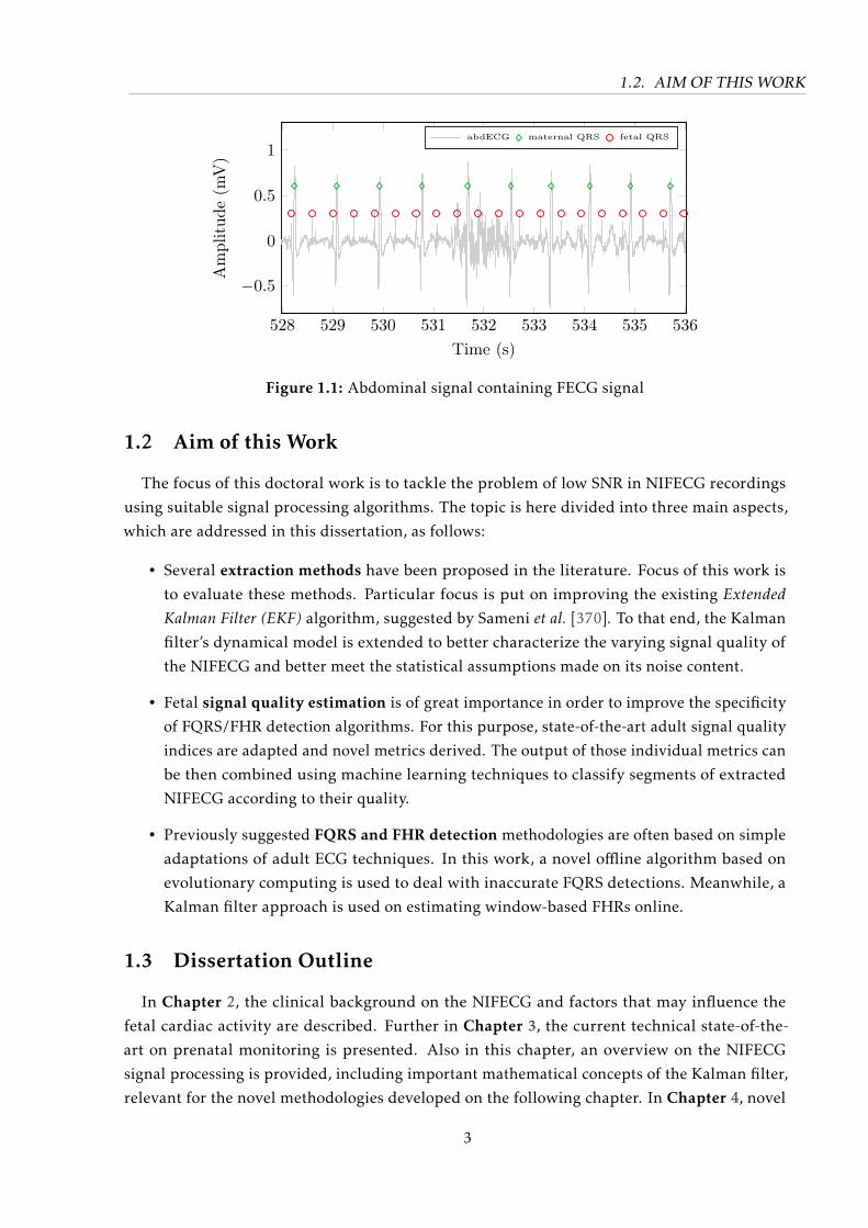
1.1 Abdominal signal containing FECG signal . . . . . . . . . . . . . . . . . . . . . . 3
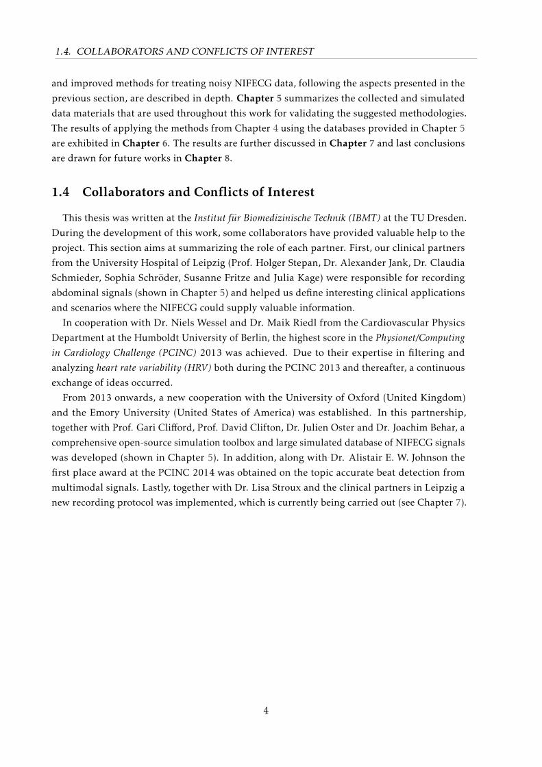
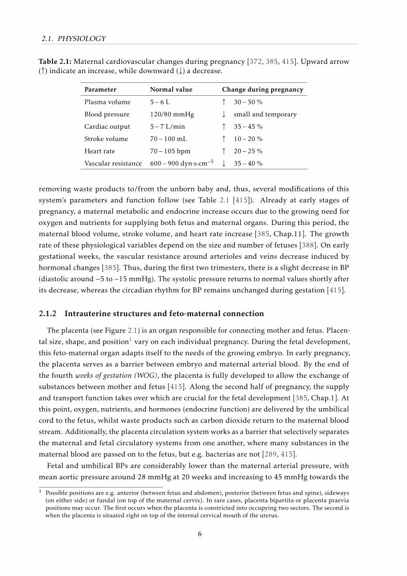
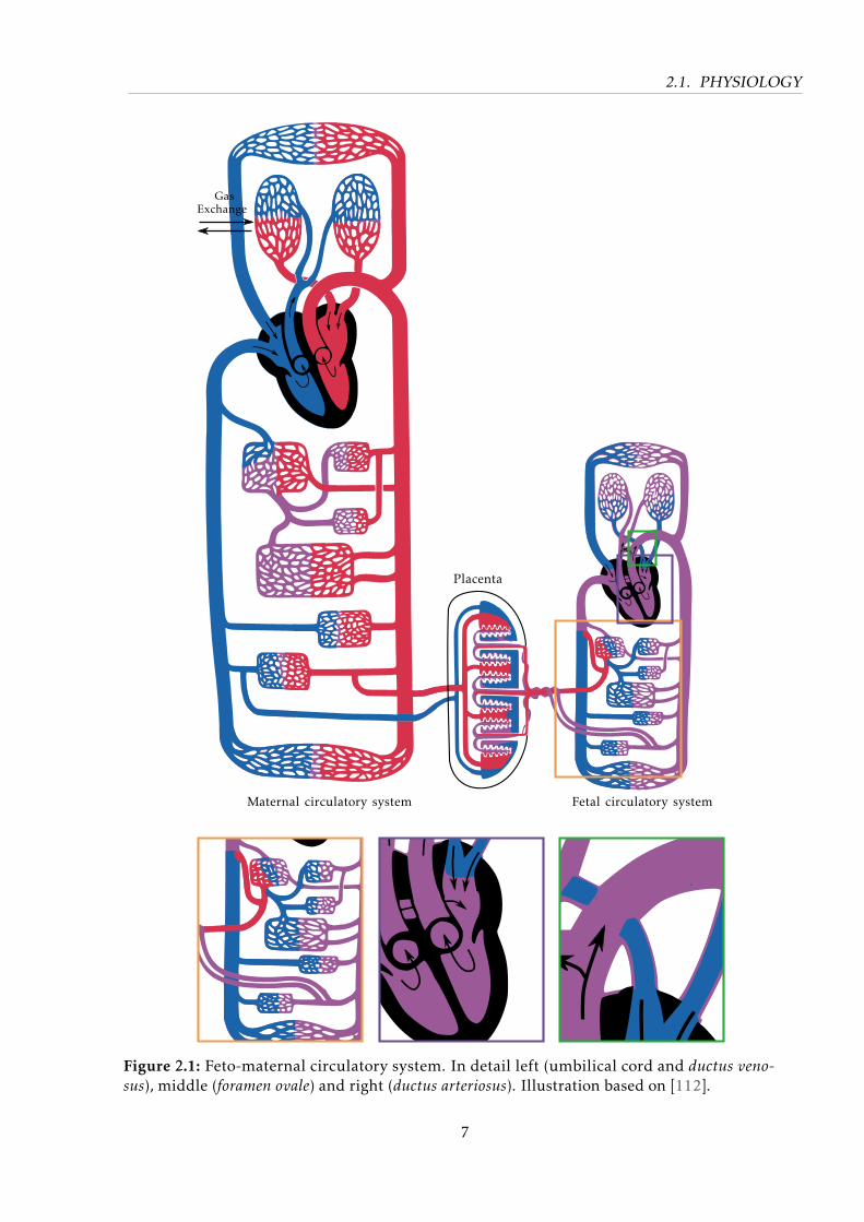
2.1 Feto-maternal circulatory system. . . . . . . . . . . . . . . . . . . . . . . . . . . . 7
2.2 Exemplary beat demonstrating morphological features . . . . . . . . . . . . . . . 17
3.1 NIFECG recording principle . . . . . . . . . . . . . . . . . . . . . . . . . . . . . . 24
3.2 Predominant sources present in abdominal measurements. . . . . . . . . . . . . 25
3.3 Different electrode configurations present in the literature. . . . . . . . . . . . . 28
3.4 Indirect techniques for FECG extraction and their main characteristics . . . . . . 33
3.5 Representation of Bayesian estimation based on prior observations . . . . . . . . 38
3.6 Signal processing work-flow for NI-FECG extraction using T Sekf. . . . . . . . . . 52
3.7 Kalman filter ECG modelling algorithm . . . . . . . . . . . . . . . . . . . . . . . 53
3.8 KF modelling using real recording. . . . . . . . . . . . . . . . . . . . . . . . . . . 54
3.9 FECG extraction using EKF algorithm . . . . . . . . . . . . . . . . . . . . . . . . 56
3.10 Exemplary fetal heart rate tachogram. . . . . . . . . . . . . . . . . . . . . . . . . 62
3.11 Signal processing steps for morphological analysis. . . . . . . . . . . . . . . . . . 65
4.1 Low-pass filters for quadratic spline wavelet. . . . . . . . . . . . . . . . . . . . . 71
4.2 Stationary wavelet transform fitting. . . . . . . . . . . . . . . . . . . . . . . . . . 72
4.3 Comparison of best performing fitting methods . . . . . . . . . . . . . . . . . . . 74
4.4 State’s evolution using the EKF24 . . . . . . . . . . . . . . . . . . . . . . . . . . . 75
4.5 Example of covariance matrix adaptation using EKF2 . . . . . . . . . . . . . . . 77
4.6 Representation of the xSQI metric . . . . . . . . . . . . . . . . . . . . . . . . . . . 83
4.7 Qualitative example of different sub-functions used for defining the fitness function. 84
4.8 Evolutionary algorithm at different iteration steps . . . . . . . . . . . . . . . . . 85
4.9 Example of newly proposed SQIs on good and bad quality extracted segments . 89
4.10 Relative frequency of each class the on annotated training set and normalization
function used after classification. . . . . . . . . . . . . . . . . . . . . . . . . . . . 92
5.1 Three dipole components and resulting vectorcardiogram. . . . . . . . . . . . . . 99
5.2 Side and upper view the of volume conductor . . . . . . . . . . . . . . . . . . . . 101
5.3 Exemplary simulated signals . . . . . . . . . . . . . . . . . . . . . . . . . . . . . . 102
5.4 Electrode configuration used in this work. . . . . . . . . . . . . . . . . . . . . . . 103
5.5 Exemplary signals collected during this work. . . . . . . . . . . . . . . . . . . . . 104
5.6 Study’s population . . . . . . . . . . . . . . . . . . . . . . . . . . . . . . . . . . . . 105
5.7 Collected signals with different quality . . . . . . . . . . . . . . . . . . . . . . . . 107
ix

LIST OF FIGURES
5.8 Annotated segments for NIFECG signal quality . . . . . . . . . . . . . . . . . . . 110
5.9 Channel-by-channel overview of consensus annotations for FECG and SNR . . . 112
5.10 Post-hoc analysis for channel quality . . . . . . . . . . . . . . . . . . . . . . . . . 113
5.11 Recording’s quality across different gestational weeks . . . . . . . . . . . . . . . 113
5.12 Effect sizes across different gestational weeks . . . . . . . . . . . . . . . . . . . . 115
6.1 Detailed F1 results for FQRS detection accuracy . . . . . . . . . . . . . . . . . . . 121
6.2 Post hoc analysis for FQRS detection accuracy . . . . . . . . . . . . . . . . . . . . 122
6.3 Two exemplary segments are portrayed during which BSSica’s mixing matrix is
updated . . . . . . . . . . . . . . . . . . . . . . . . . . . . . . . . . . . . . . . . . . 122
6.4 Differences in measured FQT intervals between extracted channels and reference 124
6.5 Differences in measured FTQRS ratios between extracted channels and reference 124
6.6 Accuracy of FQT and FTQRS extraction for the different methods . . . . . . . . 125
6.7 Evolutionary QRS correction using three channels . . . . . . . . . . . . . . . . . 126
6.8 Excerpt of clinical signals extracted using ICA . . . . . . . . . . . . . . . . . . . . 127
6.9 Segments of data comprising SQI metrics . . . . . . . . . . . . . . . . . . . . . . 128
6.10 Bar graph showing the feature importance using RELIEFF . . . . . . . . . . . . . 129
6.11 Correlations amongst SQI proposed features . . . . . . . . . . . . . . . . . . . . . 130
6.12 Example multichannel FHR estimation by means of Kalman filtering using three
channels . . . . . . . . . . . . . . . . . . . . . . . . . . . . . . . . . . . . . . . . . 132
7.1 Timeline for new measurement protocol. . . . . . . . . . . . . . . . . . . . . . . . 134
7.2 Exemplary segment of new measurement protocol . . . . . . . . . . . . . . . . . 136
A.1 Signal quality annotation interface. . . . . . . . . . . . . . . . . . . . . . . . . . . 175
B.1 Java GUI used for FQRS annotation . . . . . . . . . . . . . . . . . . . . . . . . . . 178
C.1 Screenshots of recording GUI. . . . . . . . . . . . . . . . . . . . . . . . . . . . . . 180
C.2 Chages to the GUI during physiological maneuvers. . . . . . . . . . . . . . . . . 181
x

List of Tables
2.1 Maternal cardiovascular changes during pregnancy . . . . . . . . . . . . . . . . . 6
2.2 Influencing factors for the fetal heart activity . . . . . . . . . . . . . . . . . . . . 12
3.1 Available techniques in fetal heart monitoring. . . . . . . . . . . . . . . . . . . . 21
3.2 Notation used in this work. . . . . . . . . . . . . . . . . . . . . . . . . . . . . . . . 32
3.3 NI-FECG extraction algorithms. . . . . . . . . . . . . . . . . . . . . . . . . . . . . 37
4.1 Results for different fitting methods evaluated. . . . . . . . . . . . . . . . . . . . 73
4.2 Summary of fetal SQI metrics used in this work. . . . . . . . . . . . . . . . . . . 90
4.3 Fetal QRS detectors evaluated in this work. . . . . . . . . . . . . . . . . . . . . . 91
5.1 Scenarios used for simulating pregnancy’s pathophysiological events. . . . . . . 101
5.2 FECGSYN model parameters used within this work . . . . . . . . . . . . . . . . . 102
5.3 Descriptive statistics on collected data. . . . . . . . . . . . . . . . . . . . . . . . . 106
5.4 Clinical data annotation classes and definitions. . . . . . . . . . . . . . . . . . . . 108
5.5 Intra-observer and inter-observer agreement by means of Krippendorff’s alpha
statistic. . . . . . . . . . . . . . . . . . . . . . . . . . . . . . . . . . . . . . . . . . . 109
5.6 Definition of fetal peak visibility consensus . . . . . . . . . . . . . . . . . . . . . 110
5.7 Measures of dependency and bivariate association used in this study. . . . . . . 114
5.8 Correlation table for clinical data . . . . . . . . . . . . . . . . . . . . . . . . . . . 117
6.1 Case-by-case FQRS results for FECGSYNDB . . . . . . . . . . . . . . . . . . . . . 120
6.2 Results for FQRS detection accuracy and precision using the evolutionary correc-
tion algorithm . . . . . . . . . . . . . . . . . . . . . . . . . . . . . . . . . . . . . . 126
6.3 Resulting confusion matrix for the 10-fold cross validation . . . . . . . . . . . . 128
6.4 Performance comparison using proposed KF technique in terms of FHR accuracy
and precision . . . . . . . . . . . . . . . . . . . . . . . . . . . . . . . . . . . . . . . 131
B.1 Fetal QRS annotation markers used in this work . . . . . . . . . . . . . . . . . . . 178
xi


List of Abbreviations
abdECG abdominal electrocardiogram
ACC accuracy
ADC analog-digital converter
AHA American Heart Association
ALS Autocovariance Least Squares
AM Adaptive Methods
ANC Adaptive Noise Canceller
ANFIS Adaptive Neuro-Fuzzy Interference System
ANOVA Analysis of Variance
ANS autonomic nervous system
ANSI American National Standards Institute
ApEn approximate entropy
AR autoregressive
AV atrioventricular
BBI beat-to-beat interval
BMI body mass index
BP blood pressure
bpm beats per minute
BSS Blind Source Separation
BW baseline wander
cbPPG camera-based photoplethysmogram
CHD congenital heart defect
CI confidence interval
xiii

LIST OF TABLES
CTG cardiotocogram
DFA detrended fluctuation analysis
DORV double outlet right ventricle
DTW Dynamic Time Warping
DWT discrete wavelet transform
EA evolutionary algorithms
ECG electrocardiogram
EEG electroencephalogram
EHG electrohysterogram
EKF Extended Kalman Filter
EKS Extended Kalman Smoother
EM electrode motion
EMG electromyogram
EnKF Ensemble Kalman Filter
eQRS evolutionary QRS correction algorithm
ESN Echo State Network
FAMD Factor Analysis with Mixed Data
FBMs fetal breathing-like movements
FBS fetal blood sampling
FDA U.S. Food and Drug Administration
FECG fetal electrocardiogram
FECGSYNDB Fetal ECG Synthetic Database
FECGSYN Fetal ECG Synthetic Generator
FF fixed fitting
FFT fast Fourier transform
FHR fetal heart rate
FHRV fetal heart rate variability
xiv

LIST OF TABLES
FIR finite impulse response
FMCG fetal magnetocardiogram
FN false negative
FP false positive
FPO fetal pulse oximetry
FQRS fetal QRS
FQT fetal QT
FSE fetal scalp electrode
FST fetal ST
FTQRS fetal T/QRS
FV fitness value
GBF Grid-based Filter
GOF goodness of the fit
GP Gaussian Processes
GPL General Public License
GSF Gaussian Sum Filter
GUI graphical user interface
HDR heart rate detection rate
HF high-frequency
HMM hidden Markov model
HR heart rate
HRV heart rate variability
IBME Institute of Biomedical Engineering
IBMT Institut für Biomedizinische Technik
ICA Independent Component Analysis
IC independent component
IIR infinite impulse response
xv

LIST OF TABLES
ITAM Institute of Technical and Medical Equipments
IUGR Intrauterine growth restriction
IUP intrauterine pressure
KF Kalman Filter
LF/HF low to high-frequency ratio
LF low-frequency
LMS Least Mean Squares
MAE mean average error
MA muscular artifact
MAP maximum a posteriori
MECG maternal electrocardiogram
MHR maternal heart rate
ML maximum likelihood
MMSE minimum mean square error
MQRS maternal QRS
MSE mean square error
MVUE minimum variance unbiased estimator
NIFECG non-invasive fetal electrocardiogram
NMSE normalized mean square error
NSSP Nonlinear State-Space Projection
NSTDB Normal Stress Test Database
OSET Open-Source Electrophysological Toolbox
PCA Principal Component Analysis
PCG phonocardiogram
PCINC Physionet/Computing in Cardiology Challenge
PDF probability density function
πCA Periodic Component Analysis
xvi

LIST OF TABLES
PPG photoplethysmogram
PPV positive predictive value
PROM premature rupture of membranes
PVC premature ventricular contraction
RI recoding index
RLS Recursive Least Squares
RMSE root mean square error
RMSSD root mean squared differences between adjacent beat-to-beat
intervals
ROI region of interest
RSF random search fitting
SampEn sample entropy
SA sinoatrial
SDNN standard deviation of all normal beat-to-beat intervals
SE sensitivity
SGA small for gestational age
SIS Sequential Importance Sampling
SNR signal-to-noise ratio
SOMs Self-Organizing Maps
SPKF Sigma-point Kalman filter
SQI signal quality index
SQUID superconducting quantum interference device
SQUID Superconducting Quantum Interference Device
STFT Short Time Fast Fourier Transform
SVD Singular Value Decomposition
SWTF stationary wavelet transform fitting
SWT Stationary Wavelet Transform
xvii

LIST OF TABLES
TD Tensors Decomposition
TP true positive
TS Template Subtraction
UF uniform fitting
UIEKF Unknown Input Extended Kalman Filter
UKF Unscented Kalman Filter
VCG vectocardiogram
VSD ventricular septal defect
WGN white Gaussian noise
WOG weeks of gestation
xviii

List of Symbols
Greek Symbols
Symbol Description Dimensions Units
αi amplitude normalization fac-
tor for ith Gaussian kernel
R1×1 mV
αK Krippendorff’s alpha coeffi-
cient
R1×1 –
χ2 Chi-square statistic R1×1 –
δ sampling period R1×1 ms
∆θi,k phase of the ith Gaussian at
time-step k
R1×1 rad
η Correlation ratio R1×1 –
ηk random additive noise term R1×1 mV
ηθ,k Random additive noise to
phase state
R1×1 s
ηz,k Random additive noise to sig-
nal amplitude state
R1×1 s
κ Kappa agreement coefficient R1×1 –
λv Forgetting factor for weight-
ing measurement noise covari-
ance matrix
R1×1 s
λw Update coefficient for matrix
process noise covariance
R1×1 s
ω angular frequency of current
beat
R1×1 rad/s
φi position of the ith kernel in-
side template
R1×1 rad
ρ Spearman’s ρ correlation coef-
ficient
R1×1 –
τ0 Initialization time R1×1 s
xix

List of Symbols
θ phase information R1×1 rad
Roman Symbols
Symbol Description Dimensions Units
FQT fetal QT interval error R1×1 ms
˜FTQRS fetal T/QRS ratio error R1×1 –
ACC fetal QRS accuracy measure R1×1 %
E1/E4 fetal heart rate scoring statis-
tics
R1×1 bpm2
E2/E5 root mean squared error be-
tween RR intervals
R1×1 ms
F1 fetal QRS accuracy measure R1×1 %
HDR heart rate detection rate R1×1 %
MAE mean absolute distance be-
tween fetal detections
R1×1 ms
P P V positive predictive value R1×1 %
sk Single diagonal entry from in-
novation covariance matrix
R1×1 s
SE sensitivity R1×1 %
R≥0 non-negative real number – –
Z≥0 non-negative integer number – –
Fk state transition Jacobian ma-
trix
Rn×n –
Hk observation Jacobian matrix Rm×m –
Vk measurement noise Jacobian
matrix
Rm×m –
Wk process noise Jacobian matrix Rn×n –
Dk unknown input system ma-
trix
Rn×s –
Ek unknown input feedthrough
matrix
Rm×s –
Fk state transition matrix Rn×n –
Gk control input matrix Rn×m –
xx

List of Symbols
Hk observation matrix transition Rm×n –
Kk Kalman gain Rn×n –
Pk|k−1 a priori state error covariance
matrix
Rn×n –
Pk|k a posteriori state error covari-
ance matrix
Rn×n –
W mixing matrix Rn×n –
0 all zeros column vector Rn×1 –
dk unknown input Rs×1 –
uk control input Rn×1 –
vk measurement noise Rm×1 –
wk process noise Rn×1 –
xk state variable Rn×1 –
yk
observation vector Rm×1 –
ai[n] approximation at scale i
(wavelet context)
R1×1 –
bi standard deviation of ith
Gaussian kernel
R1×1 rad
Cxy spectral coherence between
x(t) and y(t)
R1×1 ∈ [0,1] –
fs sampling frequency R1×1 Hz
li[n] low-pass filter at level i
(wavelet context)
R1×1 –
Nb number of bins Z≥0 –
Nh number of harmonics N1× 1 –
Nh number of point for fast
Fourier transform
N1× 1 –
Nk number of Gaussian kernels Z≥0 –
pe percentage of agreement by
chance (Kappa statistic)
R1×1 –
pk Single diagonal entry from
state prediction covariance
matrix
R1×1 s
xxi

List of Symbols
po percentage of observed total
agreement (Kappa statistic)
R1×1 –
qk Single diagonal entry from
process noise covariance ma-
trix
R1×1 s
r Pearson’s r correlation coeffi-
cient
R1×1 –
rk Single diagonal entry from
measurement noise covari-
ance matrix
R1×1 s
Sxy cross-spectral density be-
tween x(t) and y(t)
R1×1 –
w Cohen’s w coefficient R1×1 –
X(f ) Fourier transform of signal at
frequency f
R1×1 –
xxii
And now for something completely different.
– Monty Python’s Flying Circus (1971)
1Introduction
1.1 Background and Motivation
Prenatal cardiac monitoring is an aspect of utmost importance in early detection of fetal
distress. Currently, electronic fetal heart monitoring is used on the majority of pregnancy
episodes in the developed world, whereby the analysis of fetal heart rate (FHR) is often used
to identify risk situations for both mother and fetus [129, 365]. The main reasons for this
monitoring is to rule out eventual environmental or congenital conditions that may lead to
fetal/newborn morbidity or even death. Every year, about one out of 125 babies are born with
some form of congenital heart defect (CHD) [13], which is the most common birth defect and
the leading cause of birth defect-related deaths. An estimated 2.65 million stillbirths occurred
worldwide in 2008, of which 98% occur in countries of low and middle income, with more than
45% during the intrapartum period [49, 242]. These stillbirth rates varied from 2 per 1000
(Finland) to 40 per 1000 (Nigeria and Pakistan) [242]. During 2014 in Germany, the rate of
stillbirths was 5.4 per 1000 stillbirths and neonatal (i.e. during the newborn’s first week of
life) deaths [73]. The early and more effective detection of abnormal fetal health state can help
obstetrics and pediatric cardiologists to prescribe proper medications in time, or to consider the
necessary precautions during delivery or after birth [362].
Fetal heart monitoring is not only useful for diagnosing and monitoring CHD fetuses, but
it also may improve the diagnosis of other heart-related pathologies such as hypoxia, growth
restriction and anemia. Such complications can happen prior to or during birth and may
have long lasting effects on the newborns health, if exposure is prolonged (e.g. cerebral palsy
is related to cerebral hypoxia and birth complications). As mothers progressively decide to
postpone their first pregnancy, there is a higher risk for the fetal health [143, 306]. Indeed,
increasing the effectiveness and reducing costs of prenatal monitoring on risk pregnancies is a
priority for both developed and underdeveloped worlds.
1
1.1. BACKGROUND AND MOTIVATION
The standard technique for perinatal assessment of the developing heart is the cardiotocogram(CTG). Despite being the most available mean of surveillance, CTG only provides time-averaged
mechanical information about the fetal heart. Furthermore, CTG’s interpretation is subjective
and lacks consensus amongst experts/guidelines on its interpretation. These problems in CTG’s
usage have lead to high false-positive rates in the detection of pathological patterns [298].
Therefore, instead of producing a decrease in perinatal morbidity/mortality, CTG was made
accountable for an increase in unnecessary obstetric interventions (e.g. cesarean delivery) and
in instrumental vaginal deliveries [41].
Limitations on the current techniques have instigated the pursuit for alternative fetal monitor-
ing methods over the last few decades. Particularly, because of its potential to furnish prenatal
diagnostic information, the so-called non-invasive fetal electrocardiogram (NIFECG) (see Fig. 1.1)
has become the focus of several studies [51, 92, 310, 333, 365]. Due to its higher temporal,
frequency, and spatial resolution, the NIFECG enables the monitoring of fetal QRS (FQRS)complexes in a beat-to-beat manner. Therefore, the use of sophisticated FHR/fetal heart ratevariability (FHRV) techniques is possible. FHRV parameters provide important indices in de-
termining the functional state of the autonomic nervous system (ANS) and have been associated
with diverse pathological conditions such as hypoxia (i.e. the deprivation of an adequate oxygen
supply – see Hutter et al. [196] for a complete review) and growth restriction [188]. Beyond FHR
and FHRV information, the fetal electrocardiogram (FECG) may allow a deeper characterization
of the electrophysiological activity (i.e. heart electrical conduction) by means of morphological
analysis of FECG’s signal waveform. Such a morphological analysis provides additional insights
that cannot be obtained through CTG. In contrast to CTG, NIFECG can be measured using
regular electrocardiogram (ECG) surface electrodes attached to the maternal abdomen. This
straightforward recording scheme provides considerable advantages regarding the recording
effort, which makes NIFECG a suitable technique for the ubiquitous monitoring of risk preg-
nancies. Amongst those benefits is the non-requirement of an expert supervision during data
collection1, consequent long-term recording capability of NIFECG technique, and its relative
low-cost.
Unfortunately, non-invasively recorded FECG signals are usually corrupted by many interfer-
ing noise sources, most significantly by maternal electrocardiogram (MECG) whose amplitude is
usually much greater than those of the FECG. The generally low signal-to-noise ratio (SNR) of
the resultant FECG makes the extraction (i.e. methods for separating the FECG from abdominalelectrocardiogram (abdECG) measurements) and subsequent detection of the FQRS complexes a
challenging task. Several contributions in the literature have focused on this canonical source
separation problem (see [92, 365]), however slight progress has been made. Moreover, due to
the lack of randomized clinical trials available, little is known about the nature of the NIFECG
signal and its real diagnostic value. Despite its outstanding potential, the real diagnostic value
of current NIFECG approaches have not been demonstrated to date. Consequently, its use in
clinical practice is yet restricted.
1 CTG, on the other hand, often requires medical experts to reposition the ultrasound probe.
2
1.2. AIM OF THIS WORK
528 529 530 531 532 533 534 535 536
−0.5
0
0.5
1
Time (s)
Am
plit
ude
(mV
)
abdECG maternal QRS fetal QRS
Figure 1.1: Abdominal signal containing FECG signal
1.2 Aim of this Work
The focus of this doctoral work is to tackle the problem of low SNR in NIFECG recordings
using suitable signal processing algorithms. The topic is here divided into three main aspects,
which are addressed in this dissertation, as follows:
• Several extraction methods have been proposed in the literature. Focus of this work is
to evaluate these methods. Particular focus is put on improving the existing ExtendedKalman Filter (EKF) algorithm, suggested by Sameni et al. [370]. To that end, the Kalman
filter’s dynamical model is extended to better characterize the varying signal quality of
the NIFECG and better meet the statistical assumptions made on its noise content.
• Fetal signal quality estimation is of great importance in order to improve the specificity
of FQRS/FHR detection algorithms. For this purpose, state-of-the-art adult signal quality
indices are adapted and novel metrics derived. The output of those individual metrics can
be then combined using machine learning techniques to classify segments of extracted
NIFECG according to their quality.
• Previously suggested FQRS and FHR detection methodologies are often based on simple
adaptations of adult ECG techniques. In this work, a novel offline algorithm based on
evolutionary computing is used to deal with inaccurate FQRS detections. Meanwhile, a
Kalman filter approach is used on estimating window-based FHRs online.
1.3 Dissertation Outline
In Chapter 2, the clinical background on the NIFECG and factors that may influence the
fetal cardiac activity are described. Further in Chapter 3, the current technical state-of-the-
art on prenatal monitoring is presented. Also in this chapter, an overview on the NIFECG
signal processing is provided, including important mathematical concepts of the Kalman filter,
relevant for the novel methodologies developed on the following chapter. In Chapter 4, novel
3
1.4. COLLABORATORS AND CONFLICTS OF INTEREST
and improved methods for treating noisy NIFECG data, following the aspects presented in the
previous section, are described in depth. Chapter 5 summarizes the collected and simulated
data materials that are used throughout this work for validating the suggested methodologies.
The results of applying the methods from Chapter 4 using the databases provided in Chapter 5
are exhibited in Chapter 6. The results are further discussed in Chapter 7 and last conclusions
are drawn for future works in Chapter 8.
1.4 Collaborators and Conflicts of Interest
This thesis was written at the Institut für Biomedizinische Technik (IBMT) at the TU Dresden.
During the development of this work, some collaborators have provided valuable help to the
project. This section aims at summarizing the role of each partner. First, our clinical partners
from the University Hospital of Leipzig (Prof. Holger Stepan, Dr. Alexander Jank, Dr. Claudia
Schmieder, Sophia Schröder, Susanne Fritze and Julia Kage) were responsible for recording
abdominal signals (shown in Chapter 5) and helped us define interesting clinical applications
and scenarios where the NIFECG could supply valuable information.
In cooperation with Dr. Niels Wessel and Dr. Maik Riedl from the Cardiovascular Physics
Department at the Humboldt University of Berlin, the highest score in the Physionet/Computingin Cardiology Challenge (PCINC) 2013 was achieved. Due to their expertise in filtering and
analyzing heart rate variability (HRV) both during the PCINC 2013 and thereafter, a continuous
exchange of ideas occurred.
From 2013 onwards, a new cooperation with the University of Oxford (United Kingdom)
and the Emory University (United States of America) was established. In this partnership,
together with Prof. Gari Clifford, Prof. David Clifton, Dr. Julien Oster and Dr. Joachim Behar, a
comprehensive open-source simulation toolbox and large simulated database of NIFECG signals
was developed (shown in Chapter 5). In addition, along with Dr. Alistair E. W. Johnson the
first place award at the PCINC 2014 was obtained on the topic accurate beat detection from
multimodal signals. Lastly, together with Dr. Lisa Stroux and the clinical partners in Leipzig a
new recording protocol was implemented, which is currently being carried out (see Chapter 7).
4

Obstetrician 1: Get the EEG, the BP monitor, and the AVV.
Obstetrician 2: And get the machine that goes “ping!”.
Obstetrician 1: And get the most expensive machine - in case the administrator comes.
– Monty Python’s The Meaning of Life (1983) - Part I: The Miracle of Birth
2Clinical Background
During a healthy pregnancy, a series of adaptations occur to both mother and fetus bodies.
The aim of fetal monitoring is to evaluate if these changes are related to physiological or
pathological conditions during the pregnancy. This chapter provides background information
on the current clinical state of fetal monitoring, on which this doctoral work is built. With that
in mind, Section 2.1 provides information about the fetal development that are relevant for
fetal monitoring. Meanwhile, Section 2.2 describes some complications that may benefit from
novel monitoring techniques. Background information on current approaches to interpreting
the available information about the fetal heart is presented in Section 2.3.
2.1 Physiology
The duration of a normal human pregnancy spans approximately 280 days (40 weeks),
counted from the onset of the last normal menstrual period onwards [361]. In Germany, 90% of
births occur between 37 and 42 weeks [72]. During pregnancy, several changes to both fetus
and mother’s body take place, which are briefly described in the next few sections.
2.1.1 Changes in the maternal circulatory system
The arterial blood pressure (BP) of a healthy resting adult is on average around 120/80 mmHg
[382, Chap.28], where the first value represents the systolic BP, while the second the diastolic BP.
These values vary depending on age, sex, circadian rhythm, posture, respiration and modulation
input from the ANS [382]. Changes in BP can occur slowly, e.g. during body changes due to
pregnancy, or suddenly with postural changes (e.g., orthostatic maneuvers) [415].
Amongst the various adaptations that take place during physiological pregnancies, in this
work focus is given to changes on the cardiovascular system. In this regard, throughout
the gestation the maternal cardiovascular system is responsible for providing oxygen to and
5
2.1. PHYSIOLOGY
Table 2.1: Maternal cardiovascular changes during pregnancy [372, 385, 415]. Upward arrow(↑) indicate an increase, while downward (↓) a decrease.
Parameter Normal value Change during pregnancy
Plasma volume 5− 6 L ↑ 30− 50 %
Blood pressure 120/80 mmHg ↓ small and temporary
Cardiac output 5− 7 L/min ↑ 35− 45 %
Stroke volume 70− 100 mL ↑ 10− 20 %
Heart rate 70− 105 bpm ↑ 20− 25 %
Vascular resistance 600− 900 dyn·s·cm−5 ↓ 35− 40 %
removing waste products to/from the unborn baby and, thus, several modifications of this
system’s parameters and function follow (see Table 2.1 [415]). Already at early stages of
pregnancy, a maternal metabolic and endocrine increase occurs due to the growing need for
oxygen and nutrients for supplying both fetus and maternal organs. During this period, the
maternal blood volume, stroke volume, and heart rate increase [385, Chap.11]. The growth
rate of these physiological variables depend on the size and number of fetuses [388]. On early
gestational weeks, the vascular resistance around arterioles and veins decrease induced by
hormonal changes [385]. Thus, during the first two trimesters, there is a slight decrease in BP
(diastolic around −5 to −15 mmHg). The systolic pressure returns to normal values shortly after
its decrease, whereas the circadian rhythm for BP remains unchanged during gestation [415].
2.1.2 Intrauterine structures and feto-maternal connection
The placenta (see Figure 2.1) is an organ responsible for connecting mother and fetus. Placen-
tal size, shape, and position1 vary on each individual pregnancy. During the fetal development,
this feto-maternal organ adapts itself to the needs of the growing embryo. In early pregnancy,
the placenta serves as a barrier between embryo and maternal arterial blood. By the end of
the fourth weeks of gestation (WOG), the placenta is fully developed to allow the exchange of
substances between mother and fetus [415]. Along the second half of pregnancy, the supply
and transport function takes over which are crucial for the fetal development [385, Chap.1]. At
this point, oxygen, nutrients, and hormones (endocrine function) are delivered by the umbilical
cord to the fetus, whilst waste products such as carbon dioxide return to the maternal blood
stream. Additionally, the placenta circulation system works as a barrier that selectively separates
the maternal and fetal circulatory systems from one another, where many substances in the
maternal blood are passed on to the fetus, but e.g. bacterias are not [289, 415].
Fetal and umbilical BPs are considerably lower than the maternal arterial pressure, with
mean aortic pressure around 28 mmHg at 20 weeks and increasing to 45 mmHg towards the
1 Possible positions are e.g. anterior (between fetus and abdomen), posterior (between fetus and spine), sideways(on either side) or fundal (on top of the maternal cervix). In rare cases, placenta bipartita or placenta praeviapositions may occur. The first occurs when the placenta is constricted into occupying two sectors. The second iswhen the placenta is situated right on top of the internal cervical mouth of the uterus.
6
2.1. PHYSIOLOGY
Maternal circulatory system Fetal circulatory system
Placenta
GasExchange
Maternal circulatory system Fetal circulatory system
Placenta
GasExchange
Maternal circulatory system Fetal circulatory system
Placenta
GasExchange
Maternal circulatory system Fetal circulatory system
Placenta
GasExchange
Figure 2.1: Feto-maternal circulatory system. In detail left (umbilical cord and ductus veno-sus), middle (foramen ovale) and right (ductus arteriosus). Illustration based on [112].
7
2.1. PHYSIOLOGY
end of gestation [414]. According to Peter and Miller [328, p.83], a major part of the blood
pressure fall occurs in the uteroplacental arteries due to its flow resistance. During the course
of pregnancy, this resistance decays causing an increase in maternal blood flow. In physiological
pregnancies approximately 450-600 mL of maternal blood flows through the placenta (ca. 10%
of the total blood volume). As in any other organ, the magnitude of blood flow in the placenta is
determined by the driving pressure (maternal BP) and the vascular resistance (uteroplacental).
Although intrafetal umbilical vessels are innervated, it is believed that the extrafetal cord and
placenta lack innervations. Therefore, neural mechanisms for regulation of placental perfusion
are believed to be irrelevant [328, p.179]. On the other hand, increased uterine blood flow is
essential to meet metabolic demand from the growing uterus as well as the placenta and fetus
[293]. Despite taking part on the body’s general vascular regulation, there is no evidence that
the uterus itself possesses an auto-regulation mechanism for vasoconstriction. For this reason,
minimalistic changes in the maternal BP are expected to have a large and direct effect on the
uterine perfusion, therefore on the fetal supply. [385, 415, Chap.11].
The uterine perfusion is influenced by hormonal (e.g. cortisol/catecholamines) changes
during pregnancy [365, 385, Chap.11]. For instance, the fetus influences the provision of
maternal nutrients via the placental production of hormones that regulate maternal metabolism.
Meanwhile, the placenta may respond to the fetal endocrine signals to increase transport of
maternal nutrients by growth of the placenta, by activating transport systems and producing
placental hormones to influence maternal physiology and even behavior [293].
Several other factors may influence the placental function and play a role in the fetal develop-
ment, such as maternal drug intake, placental or fetal defects (e.g. genetic disorders). The reader
is referred to [293] for a review. A reduction of the uteroplacental circulation may result in fetal
hypoxia and growth restriction while severe reductions may result in embryo/fetal death [289].
Some of the pathologies that lead to placental insufficiency are further described in Section 2.2.
2.1.3 Fetal growth and presentation
During the first trimester of pregnancy, the organogenesis takes place. After this period,
the underlying structures for larger organs (e.g. brain, eyes, and heart) are present [289, 415].
During the fetal period (from 9th WOG onwards), maturation of tissues and organs, as well as
a rapid growth, occur. This growth is characterized by a slowdown in the head growth and
increase in body development, where the fetus weight increases from tens of grams to a couple
kilograms and the sitting height from approximately 5 to 35 cm. During the fourth and fifth
months, the fetus increases in size while most of the weight gain occurs in the last 2.5 months
of gestation. During fetal prenatal monitoring, ultrasound assessment of the head, abdominal
and femur lengths allow an estimate for the fetal development [361]. This diagnostic is relevant
since the deprivation on the supply of nutrients for the fetus through the placenta may lead
to a condition called Intrauterine growth restriction (IUGR) (see Section 2.2.2). The lungs start
developing at the fifth WOG and are complete at late fetal stages. At the end of the 26th WOG,
the thin-walled terminal sacs are developed and the lung tissue is vascularized, which means
8
2.1. PHYSIOLOGY
that ex-utero respiration would be possible. From this point of the gestation onward, premature
newborns have a higher chance of survival given that intensive care is provided [289, Chap.10].
A fetus in-utero can obviously not breath. However, as consequence of the ANS development
(described in Section 2.1.5) and as part of the lungs’ maturation process, fetal breathing-likemovements (FBMs) can be observed from the 10th WOG onwards [172, 198]. During these
intermittent FBMs, lungs contract with amniotic fluid which is essential for the stimulation
of lung development [230]. Approximately 30 % of those movements occur during rapid eye
movement sleep [289, Chap.10]. According to Blackburn [65, Chap.10], FBMs start rapid and
irregular (occurrence around 6 % the time by 19 WOG) and become slower and more regular
weeks before delivery (around 30 % to 40 % the time at rates around 30-70 breaths per minute).
During the first and second trimesters of pregnancy, the fetuses can move with relative ease
within the uterus and have no specific presentation. This movement can be felt by the mother
from the 5th month on. According to Stinstra [409], fetuses move on average on every four
minutes between the 8-20th week and on every 5 min between 20-30th WOG. Around the half
of the third trimester, the fetus usually settles into a head-down position known as the vertex
presentation, which is most appropriate for birth. However, the fetus may also settle in other less
probable positions, e.g. breech, shoulder or other variants of the vertex position [16, 362, 409].
The fetus is surrounded by amniotic fluid and the uterus, moving outward the maternal
abdomen there are layers of muscle, fat, and skin, respectively. The amniotic fluid is reported to
have the best conductivity (at low frequencies and 37 °C) of all feto-maternal tissues, slightly
higher than the umbilical cord and placenta [311, 331, 409]. Nevertheless, the abdominal
volume conductor is not a steady conductor and its consistency, electrical properties and
geometry of its compartments change during pregnancy. A drastic change in the electrical
property of the feto-abdominal compartment is the appearance of the vernix caseosa in the last
trimester [431]. The vernix caseosa is well-documented white-colored waxy layer that covers the
fetus almost completely around this period. The vernix has been reported around the eyebrows
of fetus at 17 weeks and, as gestation progresses, it coverage of the fetal skin increases until the
32nd WOG, when most of the fetus is covered. From the 32nd WOG onwards the vernix slowly
dissolves, covering around 72 % infants’ body between 33-37 WOG, 38 % (for 37.1-40.9 WOG)
and 12 % (for 41.0-42.3 WOG). Thus some amount of vernix is still present on the skin at birth
for virtually all full term infants, humans being the only animal species who present it. Fetal
maturation is associated with an increased turbidity of the amniotic fluid, which is believed to
be linked to the detachment of the vernix [449]. An important remark for the present work is the
fact that the vernix has electrically insulating properties, with conductivity lower (by a factor
of approximately 1 million) than the conductivity of other involved tissues e.g. muscles and
amniotic fluid [311]. Therefore, it significantly attenuates the electrical potentials transmitted
from the fetal heart to the maternal abdomen surface [246], specially between the 28th to 32nd
weeks, when the vernix coverage is prevalent [246, 268, 329].
9

2.1. PHYSIOLOGY
2.1.4 Fetal circulatory system
The heart is the first organ structure to develop and it already carries most of its adult
functionalities after the organogenesis [202, 289, 415]. The fetal heart starts to beat in a
coordinated manner approximately 21 days after ovulation (at the end of the 5th WOG). Its
electrophysiology is believed to be very similar to the one of an adult [289]. Initially, the fetal
heart beats at around 80− 90 bpm and rises up to the end of the 9th week to 150− 170 bpm,
when the heart already attained most of its adult’s characteristics [202, 280]. Around the 15th
WOG, the average FHR slowly decays reaching 120− 160 bpm at late gestational age [334, 410].
See [119] for a complete depiction of the average FHR progression. Naturally, these absolute
values are modulated along the pregnancy by the developmental stage of the ANS amongst
several other external factors, which are further discussed in the following sections of this work.
Still, some mechanical differences between the fetal and adult circulatory systems exist. For
instance, in adults the left ventricle pumps blood through the body, while the right ventricle
pumps the poorly oxygenated blood into the lungs, where carbon dioxide is replaced by oxygen
[403]. In the fetal case, oxygenated blood is supplied by the placenta through the umbilical
vein (see Figure 2.1). For enabling the circulation of oxygen-rich blood throughout the body
and organs, three different shunts are present, namely the ductus venosus, foramen ovale and the
ductus arteriosus [409]. The first diverges ca. 80% [385] of the oxygenated blood that arrives
from the umbilical cord into semi-functional liver towards the vena cava. The foramen ovale is a
hole that connects both atria so that most blood bypasses the pulmonary circulation to the left
atria, consequently being pumped through the body by the left ventricle. The latter structure,
the ductus arteriosus, is also used to diverge blood which has reached and is pumped out of the
right ventricle from the lungs by connecting the pulmonary artery to the aorta [409]. Despite
no gas exchange being performed within the lungs, blood is pumped throughout the whole
fetal body (including lungs). After birth, the foramen ovale closes with the first seconds/minutes
and the ductus arteriosus partially closes within 10-15 hours (taking up to 3 weeks for complete
closure), and the ductus venosus usually closes within the first week. Other minor changes in the
physiology of the baby’s heart and its circulatory system take place within the first year of life
[16, 365].
2.1.5 Fetal autonomic nervous system
Human heart beats are caused by the pseudo-periodical excitation of the myocardium. When
physiological, this excitation originates on the sinoatrial (SA) node and propagates through
different structures of the heart. The nervous system is one of the earliest systems to begin to
develop, but it is the last to be completed (after birth). Due to this extensive formation process,
prolonged in-utero insults may have consequences to development of the nervous system [178].
The SA node is the primary structure of the electrical conduction system of the heart to manifest,
followed approximately 40 days later by a discernible atrioventricular (AV) node, the Bundle of
His and Purkinje fibers [29, Chap.1]. The electric impulse is usually generated by the SA node
that acts as the primary cardiac pacemaker.
10
2.1. PHYSIOLOGY
The SA node is strongly innervated by ANS’s two main functional branches: the parasym-
pathetic (i.e. nervus vagus) and sympathetic nervous system (i.e. spinal nerves). Over longer
periods of time, this autonomic innervation influences the sinus node and serves as indirect link
between the natural pacemaker with regulatory centers in the brain [202, 410]. The sympathetic
system is responsible for the physiological changes in the fight-or-flight response in the presence
of physical or psychological stress. Meanwhile, the parasympathetic system is responsible for
homeostasis, rest, and digest functions. Therefore, an elevated sympathetic activity leads to an
accelerated heart rate (HR), while an increase in parasympathetic activity to a deceleration. The
balance between these antagonist forces are responsible for the characteristic oscillations of the
beat-to-beat interval (BBI)s [276], which on the fetal case are responsible for the FHRV. In early
pregnancies, the sympathetic activity is predominant, since the nervus vagus (responsible for
parasympathetic activity) develops between the 11-20th WOG [181, 415, 465]. This fact explains
the slow decrease on average FHR during the second and third trimesters (as pointed out in the
previous section). Moreover, a second form of modulation is provided by the cholinergic and
adrenergic nerves of the SA node. The first is already evident at early stages of fetal growth,
whereas the second develops much later and is completed only some months after birth [202],
so that the FHR further sinks while the FHRV increases. Despite the intense research in the area,
the development of the ANS is not yet fully understood [410]. The modulation produced by
the ANS is influenced by multiple systems, e.g. respiratory, digestive, metabolic, baroreceptor
reflexes and input from higher functions of cerebral centers [181]. Due to this close relation-
ship between FHR/FHRV and the maturation status of the ANS, several researchers focus on
estimating the health state and development stage of the fetus through heart rate parameters.
2.1.6 Fetal heart activity and underlying factors
As mentioned in Section 2.1.4, some changes in FHR and FHRV are expected as pregnancy
progresses. Meanwhile, in Section 2.1.5, the ANS was shown to modulate these rates distinctly at
different stages of development. Indeed, several factors influence the fetal heart activity, such as
the stage of pregnancy, environmental conditions to which unborn child and mother are exposed
and individual characteristics. In order to evaluate the fetal development and its health state,
monitoring its heart activity is crucial (see Section 3.1). In Table 2.2 [276, 385], an overview of
the various factors that influence the fetal heart activity is presented. The motivation for such
regard to these factors is twofold: i) short-term oscillations of the fetal heart activity can provide
usable information about its health state; ii) disregarding some of these factors over longer time
periods may have a negative influence on study findings on the fetal development [256]. To
elucidate the complexity of the fetal heart activity, some of the aspects presented in Table 2.2
are further explained throughout this section.
For instance, uterine contractions are uterus muscular activities that take place during a large
part of the pregnancy and vary in intensity and frequency. Deficiency in the umbilical blood
perfusion due to cord compression might happen during a uterine contraction, which in current
medicine is associated with a characteristic pattern in FHR (see FHR interpretation guidelines
11

2.1. PHYSIOLOGY
Table 2.2: Influencing factors for the fetal heart activity [276, 385, Chap.33]
Influencing factorsendogenous (maternal) endogenous (fetal) exogenousblood pressure gestational age fetal movementoxygenation ANS regulation fetal pathophysiological statehumoral factors (e.g. stress) acidosis sleep arousalsbody posture hemodynamics uterine activitypharmacological congenital defectsdrug usage infectionbody temperature
[12, 296, 358]). According to these guidelines, in physiological cases, an early decelerationoccurs when uniform, repetitive and periodic slowing of FHR occurs with early onset in the
contraction, and return to baseline at the end of the contraction. Late decelerations, on the other
hand, are indicators of a pathological state, where the slowing of FHR coincides with the onset
mid-end of the contraction and its nadir occurs more than 20 seconds after the peak of the
contraction. Changes in the maternal pulmonary pressure or fetal movements may have similar
effects leading to a momentary deficiency on the exchange of oxygen and nutrients through the
placenta.
Since the normal fetal development entails FBMs, the observation of this activity is an
important clinical measure. In adult ECG, respiration has a great importance and reflects on
several HRV parameters [421], therefore, the same principle is expected to apply to FHRV.
Based on the presence or absence of fetal movement and patterns of the heart rate, Timor-
Tritsch et al. [428] and Nijhuis et al. [300] described four fetal behavioral states (namely, 1F, 2F, 3F,
4F). States are defined as coordinated relationship between different variables, such as gross or
fine motor activity, eyes, and FBMs as well as FHR patterns. Behavioral states are reproducible
from the 36th onwards [117, 300]. Nevertheless, current studies make often use of simplified
versions of the states described by Nijhuis et al. [300], particularly the states 3F and 4F rarely
occur [335, 438]. As pregnancy progresses the increased occurrence of quiet and active states
have been associated with several FHR/FHRV parameters [139, 188, 225, 241, 300, 335, 444].
Analogously to adults, fetal circadian rhythm fluctuations of the basal FHR can be observed
on the last trimester [256]. This behavior is however considered as a reaction to the circadian
changes in the maternal system. Evidence that supports this hypothesis is the fact that the
antenatal circadian rhythm becomes ultradian at birth [281]. Similarly, synchronization periods
between maternal and fetal average HR were found by [325, 349, 441, 444]. The latter suggested
that this association is due to the maternal respiration. To confirm this hypothesis, Van Leeuwen
et al. [443] described a higher incidence of such synchronization epochs when mothers exert a
higher breathing rate. However, the exact cause for such behavior is still controversial, usually
being attributed to heart sounds, since external stimuli such as vibroacoustic stimulation (e.g.
music or speech) can affect FHRV [25, 276, 444]. A discussion on this topic is present in [199].
Moreover, it has been shown that psychological factors such as maternal stress [115], anxiety
[226, 285], relaxation [116] or emotive state [285] can influence FHR/FHRV [444]. For instance
12
2.2. PATHOLOGY
[285] demonstrated a correlation between maternal anxiety score and basal FHR. In this study,
a significant effect for the patient group with low level of anxiety was related to an increase in
maternal BP, which could incur in changes in the FHR. Additionally, there was an increase in
the breathing rate of both groups, so that not only the acute emotional reaction but also the
respiratory influence caused by the distress is plausible.
2.2 Pathology
Many complications during antenatal and intrapartum periods may lead to fetal hypoxia.
Despite the various fetal compensatory mechanisms that take place, if hypoxia is prolonged,
it can lead to acidosis (i.e. an increased acidity in the body fluids). Severe and acute acidosis
are associated with significant morbidity (e.g. irreversible neurological damage) and mortality
[4, 67, 196]. Hypoxia effectively reduces the energy storage available for repolarization of the
myocardial cells, resulting in a changes on the FHR, FHRV and FECG waveforms [11]. Exces-
sive uterine contractions are the leading cause of hypoxia, since they may decrease placental
perfusion as well as compress the umbilical cord [38].
In this work, focus is put on three pathological conditions that are related to hypoxia. These
conditions are briefly described along the next sections and their relationship with abnormal
heart rate/morphological parameters (e.g. FHRV metrics) is hypothesized.
2.2.1 Premature rupture of membrane
Premature rupture of membrane (PROM) refers to rupture of the fetal membranes prior to the
onset of labor irrespective of gestational age. According to Caughey et al. [77], preterm PROM
complicates 2% to 20% of all deliveries and is associated with 18% to 20% of perinatal deaths.
There are several factors may promote PROM, such as antepartum vaginal bleeding, direct
abdominal trauma, smoking, drug use, low body mass index (BMI), intra-amniotic infection
and multiple pregnancy. After the occurrence of PROM, delivery is recommended when the
risk of ascending infection is greater than the risk of prematurity [77]. In early preterm PROM
patients (< 28 WOG) a lower amount of amniotic fluid (oligohydramnios) is a complicating
factor because at these stages of pregnancy it may prevent respiratory breathing movements,
therefore retarding the pulmonary growth [230]. Oligohydramnios is also associated with cord
compression and, subsequently, with fetal hypoxia [263, 410]. Moreover, there is an increased
risk of infection for both mother and fetus during this period, therefore preterm patients are
usually admitted to hospitals and closely monitored until birth.
Particularly for patients below the 28th WOG, treatments are generally more conservative
and the pregnancy is usually sustained as far as possible [385, Chap. 25]. During this period,
intermittent recordings of the FHR, together with the assessment of amniotic fluid volumetry,
amniocentesis (to exclude intra-amniotic infection) and administration of antenatal corticos-
teroids (for accelerating fetal lung maturation [351]) and broad-spectrum antibiotics (for avoid-
ing infections) [77]. From the 32nd week onwards, a more active procedure is adopted, and
13
2.2. PATHOLOGY
induced labor is beneficial for both mother and fetus [385, Chap. 25]. The German guidelines
for the treatment of PROM patients are available at [36].
2.2.2 Intrauterine growth restriction
Intrauterine growth restriction (IUGR) describes a decrease in fetal growth rate that prevents
an infant from obtaining its complete growth potential (i.e. its genetically predetermined size)
[69, 266]. IUGR does not denominate a disease per se, but rather a manifestation of many
possible fetal and maternal disorders [347]. Pregnancies affected by IUGR pose a major public
health problem affecting from 5% to 7% of all pregnancies [69] since they are also associated
with risk of hypoxia increased neonatal morbidity and mortality. In addition, it may increase
the risks for the development of hypertension, diabetes, coronary heart disease and stroke in
adulthood [347, 435].
In prenatal medicine, the estimated fetal weight is most commonly measured using 2D-
ultrasound [435]. However, according to Resnik [347], there is no consensus on what limits
should be used to define a small for gestational age (SGA) fetus/newborn. The most commonly
used definition is a birth weight less than the 10th percentile for a given gestational age [347,
385, 435]. Several standard curves for fetal growth have been suggested in the literature, but it
has to be kept in mind that fetal weight depends on several socioeconomic factors. That is, a
small fetus/newborn may merely represent the tail of the normal distribution without actually
having had any growth restriction. In order to differentiate between SGA fetuses2 and the
pathological state of IUGR, additional tests using Doppler velocimetry are required to examine
the umbilical and uterine arteries.
There are two types of IUGR, namely symmetric and asymmetric. Symmetric growth re-
striction is characterized by fetuses with smaller skeletal and head dimensions as well as
abdominal circumference. This variant is considered to be indicative of an early intrinsic
impairing condition, e.g.chromosomal abnormalities and congenital malformations. In those
cases, growth is symmetrically impaired due to its occurrence during cell division in the first
or second trimesters. Symmetric IUGR leads to a underdevelopment of the ANS (described in
Section 2.1.5). In contrast, asymmetric IUGR is usually a consequence of exogenous factors,
such as inadequacy on the availability of substrates for the fetal metabolism through the pla-
centa. This disorder takes place later in pregnancy when fetal growth occurs primarily by an
increase in cell size rather than cell number [69, 347, 410]. There is a strong association between
IUGR, chromosomal disorders and congenital malformations. Moreover, intrauterine infections,
maternal vascular diseases and maternal under nutrition may favor IUGR [69, 266]. Likewise,
chronic hypoxia (high altitudes) associated with placental insufficiency plays a key role in the
etiology of IUGR [196]. Nevertheless, the pathophysiological processes that lead to IUGR are
not fully understood, and there is a lack of agreement on guidelines for managing this condition
[81, 266, 294].
2 SGA just refers to the fact that the fetus is small, which may be due to genetic reasons such as small parents. Whennutrition is not satisfactory and there is an abnormal amount of amniotic fluid, IUGR is likely to be present.
14
2.3. INTERPRETATION OF FETAL HEART ACTIVITY
2.2.3 Fetal anemia
Anemia describes a decrease on the density of erythrocytes (i.e. red blood cells) in the
peripheral blood system. Erythrocytes’ cytoplasm are rich in hemoglobin, an iron-containing
molecule which can easily be bound with oxygen [382, Chap.23]. In pregnant women, the plasma
volume increase (mentioned in Section 2.1.1) is usually more expressive than the multiplication
of red blood cell mass, which results in a “physiological anemia” caused by hemodilution
[372, 388]. However, since these quantities widely vary from pregnancy to pregnancy, the
distinction between physiological and pathological cases is not straightforward [388].
The most common cause of fetal anemia is a pre-existing iron deficiency or other minerals
such as folate or vitamin B12, necessary for the production of hemoglobin [385, Chap. 18].
Another cause is the immunoreaction from the mother to the fetal antigens, known as Rhesus-
factor incompatibility. Such incompatibilities generate a high probability of developing fetal
anemia (alloimmune-induced hemolytic anemia) of up to 20%-25% the cases [385]. Severe
cases of anemia may lead to hydrops fetalis [259], a condition characterized by an excess of
amniotic fluid (polyhydramnios) and the accumulation of fluids in different fetal compartments
[385, Chap. 18]. Moreover, due to the low blood oxygen levels, the fetal heart needs to pump
a greater volume of blood, which may cause congested heart failure [259]. Anemia diagnosis
is performed through maternal blood sampling, ultrasound (to exclude hydrops or fetal heart
failure), amniocentesis (invasive sampling the amniotic fluid) and fetal blood sampling. If the
anemia is severe, treatment may include fetal intrauterine blood transfusion [455]. Since the fetal
oxygen transport is deficient, anemia may lead to hypoxia. In fact, some FHR sinusoidal patterns
are associated with severe anemia and hydrops [44]. For this reason, long-term monitoring of
these patients is desirable.
2.3 Interpretation of Fetal Heart Activity
Overall, fetal heart monitoring follows the advances in adult cardiac assessment. As such, it
may be divided into the analysis of the FHR and the analysis of morphological features of the
FECG signal3. For completeness, in this section, a brief summary of those current approaches is
presented.
2.3.1 Summary of clinical studies on FHR/FHRV
The FHR is qualitatively evaluated based on the visual inspection of its trace along with mea-
sures of intrauterine pressure (IUP) in clinical routines. By means of these traces, categorization
with respect to baseline heart rate and its variability, accelerations and decelerations as well
as sinusoidal patterns are carried out (see [39, 41, 295] for reviews). A number of guidelines
for interpretation of these traces have been released and updated e.g. [12, 356, 358]. More
precise computerized quantification of heart rate changes were further proposed [105] and
3 Obviously, morphological analysis of the FECG only applies when electric/magnetic principles are used in datacollection.
15
2.3. INTERPRETATION OF FETAL HEART ACTIVITY
augmented the evaluation of such traces [39, 446]. However, due to the lack of universally
accepted guidelines and poor inter and intra-observer agreements (even in cases where guide-
lines are accepted amongst clinicians) the effectiveness of current assessment techniques has
been strongly criticized [8, 44, 62, 371]. This led researchers to look for alternative automated
methods of quantifying those changes in the FHR.
For adults, the heart rate fluctuations (i.e. HRV) has been shown to be a strong, independent
predictor of future health problems [391]. Different metrics for adult HRV have been proposed
over the past 60 years, which can be divided into temporal (e.g. standard deviation of allnormal beat-to-beat intervals (SDNN) or root mean squared differences between adjacent beat-to-beatintervals (RMSSD)), spectral (e.g. low-frequency (LF) or high-frequency (HF) content as well as lowto high-frequency ratio (LF/HF) ratio) and nonlinear techniques (e.g. approximate entropy (ApEn),sample entropy (SampEn) and detrended fluctuation analysis (DFA)). A rich literature is available
on that topic, including a well-known guideline [421]. However, the U.S. Food and DrugAdministration (FDA) withdrew its support to HRV being used as a clinical parameter in 1993,
due to the lack of consensus on its efficacy [93]. Still, HRV is the focus of ongoing research,
where novel methods are constantly being proposed. Such studies focus on HRV modulating
parameters such as the length of the window around the signal of interest, preprocessing filters
used, age and gender of subject, physical and psychological conditions, sleep-awake cycles,
respiration and effect of drugs amongst others have been intensively investigated [317]. A
historical perspective on HRV is available in [64] and an analysis of signal processing algorithms
on [86]. Despite the extensive literature on adult HRV, there is to date no general agreement
about how to characterize or interpret the short and long-term oscillations of the HR.
The same discussion is applicable for FHRV parameters, which usually are adaptations of
the adult algorithms to consider the higher HR and slightly different spectral content. In this
scope, several works are available on the fetal field using several parameters [79, 84, 134, 135,
137, 146, 157, 185, 188, 240, 386, 393, 427]. A review on some of these parameters is provided
in [410]. Motivated by the physiological basic assumptions presented in Section 2.1.6, the main
focus of FHRV research has been:
• evaluating the fetal ANS maturation or brain age [146, 153, 188, 240, 313, 386, 394, 427,
445, 456]
• distinguishing between IUGR and physiological pregnancies [84, 135, 136, 290]
• correlating FHR/FHRV parameters with fetal acidosis [140, 141, 323, 437, 457]
• synchronization between maternal and fetal heart rates [349, 442–444]
• classification of fetal behavioral states [139, 188, 190, 241, 438]
• effect of maternal physical (e.g. exercise [32, 271]) and psychological (e.g. stress [115] and
anxiety [284, 285]) on fetal heart activity
Regardless of how many studies have investigated the FHRV, the vast majority of those works
are very limited in terms of number of subjects/patients and pathophysiological conditions.
16
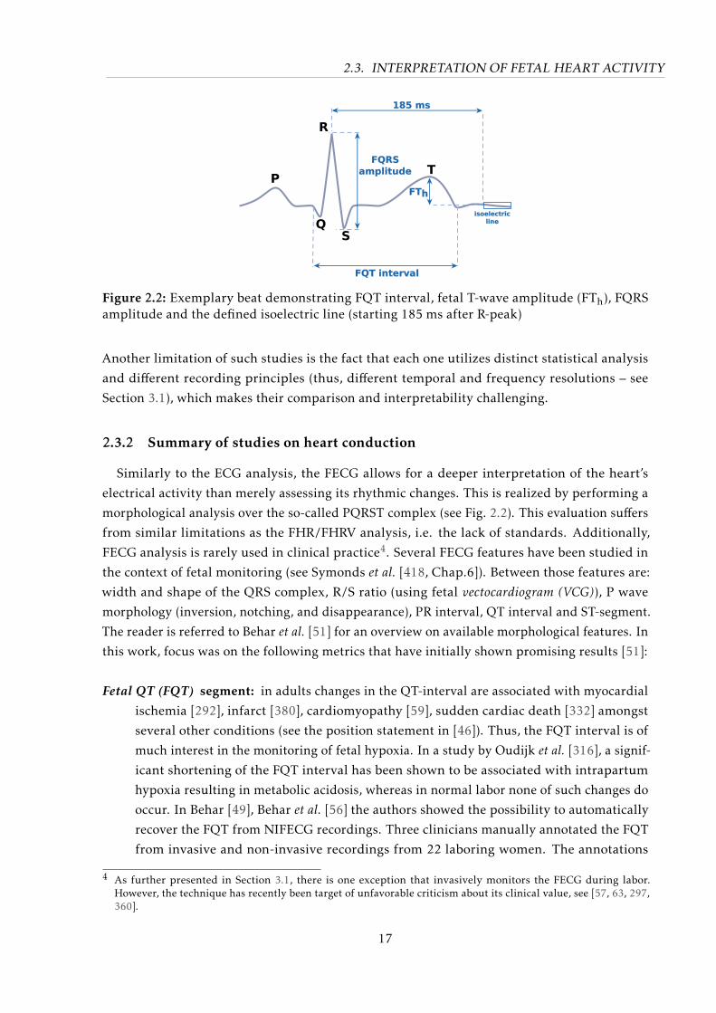
2.3. INTERPRETATION OF FETAL HEART ACTIVITY
P
QS
R
T
FQT interval
FTh
185 ms
isoelectric
line
FQRS
amplitude
Figure 2.2: Exemplary beat demonstrating FQT interval, fetal T-wave amplitude (FTh), FQRSamplitude and the defined isoelectric line (starting 185 ms after R-peak)
Another limitation of such studies is the fact that each one utilizes distinct statistical analysis
and different recording principles (thus, different temporal and frequency resolutions – see
Section 3.1), which makes their comparison and interpretability challenging.
2.3.2 Summary of studies on heart conduction
Similarly to the ECG analysis, the FECG allows for a deeper interpretation of the heart’s
electrical activity than merely assessing its rhythmic changes. This is realized by performing a
morphological analysis over the so-called PQRST complex (see Fig. 2.2). This evaluation suffers
from similar limitations as the FHR/FHRV analysis, i.e. the lack of standards. Additionally,
FECG analysis is rarely used in clinical practice4. Several FECG features have been studied in
the context of fetal monitoring (see Symonds et al. [418, Chap.6]). Between those features are:
width and shape of the QRS complex, R/S ratio (using fetal vectocardiogram (VCG)), P wave
morphology (inversion, notching, and disappearance), PR interval, QT interval and ST-segment.
The reader is referred to Behar et al. [51] for an overview on available morphological features. In
this work, focus was on the following metrics that have initially shown promising results [51]:
Fetal QT (FQT) segment: in adults changes in the QT-interval are associated with myocardial
ischemia [292], infarct [380], cardiomyopathy [59], sudden cardiac death [332] amongst
several other conditions (see the position statement in [46]). Thus, the FQT interval is of
much interest in the monitoring of fetal hypoxia. In a study by Oudijk et al. [316], a signif-
icant shortening of the FQT interval has been shown to be associated with intrapartum
hypoxia resulting in metabolic acidosis, whereas in normal labor none of such changes do
occur. In Behar [49], Behar et al. [56] the authors showed the possibility to automatically
recover the FQT from NIFECG recordings. Three clinicians manually annotated the FQT
from invasive and non-invasive recordings from 22 laboring women. The annotations
4 As further presented in Section 3.1, there is one exception that invasively monitors the FECG during labor.However, the technique has recently been target of unfavorable criticism about its clinical value, see [57, 63, 297,360].
17
2.4. CHAPTER SUMMARY
were fused, and the errors between reference and automated detection were found to be
in a similar range to adult QT-analysis.
Fetal ST (FST) segment: it is believed that an elevation of the FST segment and T wave identi-
fies hormone-induced fetal heart muscle responding to hypoxia, where a deviation from
the baseline indicates a pathological response [11]. For this reason, fetal monitoring could
greatly benefit from FST analysis. However, the ST segment delineation involves the
detection of the end of the T-wave and J-point, which even in adult ECG is a challenging
task. Due to the considerably lower amplitudes and surrounding noise, the FST is hardly
attainable. An alternative is to use the fetal T/QRS (FTQRS) ratio (as follows) as a proxy
for the FST elevation.
Fetal T/QRS (FTQRS) ratio : FTQRS was demonstrated to be a proxy for the ST segment us-
ing animal models by Greene et al. [165], where the authors examined 10 chronically
instrumented fetal lambs at 115 days to term. The study showed that the normal FTQRS
ratio was lower than 0.30, whereas it was in the range of 0.17 to 0.59 for eight of the
lambs after inducing hypoxia and reverted to normal with normoxia. However, studies
[57, 63, 297, 360] suggest that the FTQRS as proxy for the FST level is either not accurate
enough, or that it does not provide meaningful information for fetal monitoring (see
Section 3.1).
Regarding the difficult task of segmenting the largely unexplored FECG beats, the duration
of such intervals highly depend on the gestational age and projection of the fetal heart (i.e.
electrode configuration), and should be taken into consideration. Since no standard is available
for morphological analysis, clinical considerations from the current studies have to be analyzed
with caution. Symonds et al. [418] concluded in 2001 that “The issue of the value of current
use of the FECG morphological characteristics and time intervals for the prediction of fetal
compromise remains promising but unresolved”. As Behar et al. [51] pointed out: 15 years later
the problem remains unresolved.
2.4 Chapter Summary
In this chapter, an overview on the main pathophysiological influencing factors to the fetal
heart activity were presented on Sections 2.1 and 2.2). In Section 2.3, the current antepartum
clinical standards for interpreting the cardiac activity of the fetus were introduced. In the
following chapter, the state-of-the-art on techniques for prenatal diagnostic (i.e. data acquisi-
tion) are presented. Particular focus is put on the NIFECG technique’s signal acquisition and
processing methods to enable its analysis.
18

All sorts of computer errors are now turning up. You’d be surprised to
know the number of doctors who claim they are treating pregnant men.
– Isaac Asimov, quoted in Des MacHale, “Wit” (2003)
3Technical State of the Art
In the previous chapter, clinical background information on the fetal development and
cardiac activity was presented. The current chapter is mainly divided into two part, namely
signal acquisition and processing. The first, comprises diagnostic techniques for prenatal
monitoring devices available (Section 3.1) and NIFECG signal acquisition (Section 3.2). The
latter, i.e. NIFECG signal processing, is the focus of this work and is investigated in depth
within this chapter. MECG suppression / FECG extraction is presented throughout Section 3.3,
where the method of choice (i.e. the Kalman filter) is discussed extensively in Sections 3.3.2
to 3.3.4. Further in Sections 3.4 to 3.6, techniques to perform and evaluate FQRS detection,
FHR estimation, and FECG morphological analysis are showed. Lastly, in Section 3.7, the major
signal processing challenges in fetal electrocardiography are summarized.
3.1 Prenatal Diagnostic and Measuring Technique
3.1.1 Fetal heart monitoring
Monitoring methods for the fetal heart activity may be divided into invasive (i.e. used during
labor) and non-invasive (i.e. antepartum/intrapartum periods). Table 3.1 shows an overview of
the available methods, which are further described throughout this section. The first works in
fetal heart rate monitoring emerged during the 19th century and dealt with the auscultation of thefetal heart sounds. By using the wooden stethoscope introduced in 1816 by René Laennec, Pinard
suggested the intermittent auscultation of the FHR in prenatal care in 1895 [408]. Early works
associated a slow return of the FHR to its baseline after a deceleration with “fetal sufferance” and
that head compression produced bradycardia [418, Chap.2]. This rudimentary 120 years-old
technique, was still the most often used method until the 1960’s [385, Chap.33] and is still in
use in developing countries and in resource-poor settings.
Recording the heart sounds using electronic amplification (i.e. collected using a microphone),
19

3.1. PRENATAL DIAGNOSTIC AND MEASURING TECHNIQUE
the so-called phonocardiogram (PCG), was first suggested at the end of the 19th century. However,
the presence of several noise sources (e.g. intestines and veins sounds, external noise, and
fetal movements) have rendered the method impracticable [385, Chap.33]. Nevertheless, the
technique substituted auscultation using stethoscopes until the 1960s, when its sensitivity began
to be questioned [224]. Still, equipment based on PCG technology continue to be released, such
as the Sensa monitor (Nuvo Group, Tel Aviv, Israel).
In the 1960s electronic monitoring of the FHR by means of Doppler ultrasound became
available and its use rapidly disseminated. This recording of the FHR combined with the
recording of uterine activity by an external pressure transducer (i.e., the IUP), constitutes the
modern CTG [385, Chap.33]. As mentioned in Section 2.3.1, visual inspection of the FHR is
subjective and has lead to high false-positive rates in the detection of pathological patterns [298].
Moreover, recent studies found no decrease in perinatal mortality or cerebral palsy associated
with the use of CTG, aside from a potential reduction in neonatal seizures. On the contrary,
CTG was associated with an increase in unnecessary obstetric interventions such as cesarean
delivery (63% increase) and in instrumental vaginal deliveries (15% increase) [8, 39, 41, 358].
Furthermore, the side effect of long-term ultrasound exposure on the fetus is not completely
understood, and there is a risk of provoking the heating of fetal tissues [45, 92, 411]. For this
reason, the non-invasiveness of the CTG technique should be contested. These limited benefits
provided by CTG have instigated further research on alternative techniques for fetal monitoring.
For instance, hand-held Doppler ultrasounds have recently gained researchers’ interest as
a low-cost method for under-developed countries [270, 413]. However, due to considerable
susceptibility to noise and the need for directing the ultrasound probe towards the fetal heart at
all times, it is usually used as an intermittent auscultation method such as the Pinard stethoscope
and PCG (see [244] for a review of these methods and guidelines). Overall, acoustic signals such
as PCG and Doppler methods have the benefit of providing means for obtaining cardiac valves
opening and closure times, which is under current research in adult [406] (using low-cost PCG)
and fetal monitoring [270] (using hand-held Doppler).
During late stages of labor, a simple pulse oximeter can be attached to the fetal cheek (i.e.
invasively). Theoretically, the so-called fetal pulse oximetry (FPO) provides benefits over other
techniques since in addition to fetal pulse rate, it may also serve as a proxy for oxygen saturation
and tissue perfusion [114]. Despite initial reports about its usefulness [114, 261], a Cochrane
study [122] analyzing four trials rapidly criticized the technique for not reducing cesarean rates
when assisting CTG or increasing fetal and maternal outcomes.
Another non-invasive method for assessing the fetal cardiac activity is the fetal magneto-cardiogram (FMCG). The FMCG measures the magnetic flux density which emanates from
the heart to the surroundings of the maternal abdomen. Due to the low magnitude of these
magnetic fields (BFECG ≈ 10−12 T , i.e. several of orders of magnitude weaker than earth’s
magnetic field) and necessity for substantial noise reduction, highly sensitive SuperconductingQuantum Interference Device (SQUID) sensors are required. For this reason, the FMCG is usually
measured by a large equipment (i.e. short-term only) within a magnetically shielded room and
using several channels (ranging up to a couple hundred channels). The FMCG is well-suited
20

3.1. PRENATAL DIAGNOSTIC AND MEASURING TECHNIQUE
Tab
le3.
1:A
vail
able
tech
niq
ues
infe
talh
eart
mon
itor
ing
[51,
92,3
29].
Ap
pro
ach
esba
sed
onm
agn
etic
and
elec
tric
pri
nci
ple
sm
ayp
rovi
de
info
rmat
ion
onth
eca
rdia
cco
ndu
ctio
n,w
hile
acou
stic
ones
onva
lve
open
ing/
clos
ing
tim
es.A
bbre
viat
ions
stan
dfo
r:St
and
.=
stan
dar
diz
edan
alys
is;I
nvas
.=in
vasi
vem
eth
od;I
ntr
ap.=
intr
apar
tum
;CT
G=
card
ioto
cogr
am;F
CM
G=
feta
lmag
net
ocar
dio
-gr
am;F
PO
=fe
talp
uls
eox
imet
ry;F
SE=
feta
lsca
lpel
ectr
ode.
Met
hod
Pri
nci
ple
Stan
d.
Inva
s.A
nte
par
tum
Intr
ap.
FHR
Cos
t†L
ong-
term
Oth
erch
arac
teri
stic
s
CT
Gm
echa
nic/
acou
stic
Yes
7‡
3(≥
20W
OG
)3
3$$§
7–
trai
ned
exp
ert
requ
ired
duri
ngre
cord
ing
–on
lysh
ort-
tim
eca
pab
le–
FHR
avai
labl
eon
win
dow
aver
ages
–ac
tive
met
hod
(ult
raso
und
irra
dia
tion
)–
pro
neto
mat
erna
l/fe
talH
Rco
nfu
sion
–se
nsib
leto
feta
l/m
ater
nalm
ovem
ent
FMC
Gm
agne
tic
No
73
(≥20
WO
G)
73
$$$
7–
mu
ltic
hann
el(
20ch
anne
ls)
–hi
ghSN
Rfo
rFE
CG
–ex
per
tp
erso
nnel
requ
ired
duri
ngre
cord
ing
–on
lysh
ort-
term
cap
able
FPO
opti
cN
o3
73
3$
7–
sing
lech
anne
lonl
y–
app
lica
tion
pos
sibl
eaf
ter
rup
ture
ofm
embr
anes
–es
tim
ate
for
feta
loxy
gen
satu
rati
onav
aila
ble
–u
sabi
lity
ofte
nqu
esti
oned
FSE
elec
tric
No
37
33
$$7
–si
ngle
chan
nelo
nly
–ap
pli
cati
onp
ossi
ble
afte
rru
ptu
reof
mem
bran
es
NIF
EC
Gel
ectr
icN
o7
3
(≥20
WO
G)¶
33
$3
–lo
wSN
Rfo
rFE
CG
–p
rese
nce
ofve
rnix
case
osa
seve
rely
redu
ces
SNR
–no
skil
led
per
sonn
elre
quir
eddu
ring
reco
rdin
g
PC
Gm
echa
nic/
acou
stic
No
73
(≥28
WO
G)
73
$7
–lo
wes
tSN
Rof
allm
etho
ds
–re
quir
esex
per
tto
loca
tefe
tus
–se
nsit
ive
tosu
rrou
ndin
gan
dga
stro
inte
stin
alno
ises
†C
ost
disp
laye
das
$=
hund
reds
ofdo
llar
s;$$
=th
ousa
nds
ofdo
llar
s;$$
$=
tens
ofth
ousa
nds
ofdo
llar
s.E
stim
ated
valu
esba
sed
onau
thor
’sbe
stof
know
ledg
e.‡
Th
eas
pec
tof
safe
tyan
din
vasi
ven
ess
onC
TG
reco
rdin
gsis
stil
lco
ntr
over
sial
and
ith
asn
otbe
end
emon
stra
ted
that
ult
raso
un
dir
rad
iati
onex
pos
ure
was
com
ple
tely
safe
for
the
fetu
s[9
2].S
eeD
uck
[120
]for
ad
etai
led
over
view
onth
eto
pic
.§
Han
d-h
eld
Dop
ple
rar
ea
low
-cos
t1-
Dva
rian
tof
the
clin
ical
lyu
sed
ult
raso
und
,who
sep
rice
son
the
tens
ofd
olla
rsra
nge.
¶A
sm
enti
oned
inSe
ctio
n2.
1.3,
betw
een
the
28th
-32nd
WO
G,t
he
vern
ixca
seos
aco
mp
lete
lyin
volv
esth
efe
tus.
Th
isla
yer
ish
igh
lyin
sula
tin
gan
dse
vere
lyre
duce
sth
efe
talS
NR
.Fro
mth
e32
ndw
eek
onw
ards
the
laye
rsl
owly
diss
olve
sfr
omth
efe
tals
kin
into
the
amni
otic
flui
d[4
09],
arou
ndth
e37
thW
OG
abou
t60
%of
the
feta
lbod
yis
free
ofth
ela
yer
[449
]
21
3.1. PRENATAL DIAGNOSTIC AND MEASURING TECHNIQUE
for clinical measurement, generally producing fetal cardiac waveforms of good quality, which
are used for diagnosing fetal cardiac conduction disorders. Despite being already available
on the mid-1970s, its popularity only increased at the beginning of the 1990s. Due to the
expensive equipment and necessity of skilled personnel to carry out measurement, its use has
been hampered [329, 330, 410]. Nevertheless, owing to its high temporal/spatial resolution and
good SNR for the fetal signal, several published works investigate FHRV metrics using FMCG
recordings, e.g. [157, 189, 190, 386, 427, 440, 443].
The FECG is the electrical equivalent of the FMCG [246] and presents a viable alternative
that can be recorded invasively or non-invasively. Invasive FECG technology, the so-called fetalscalp electrode (FSE), uses an electrode attached to the presenting part of the fetal scalp. This
electrode is fixated to the fetal skin using either a needle-like spiral electrode that penetrates
(screws into) the skin surface, or using a spring-loaded clip to skew a piece of skin. In any case,
one electrode (positive electrode) is attached to the fetus, while other is used to make contact
with the vaginal vault and cervix (negative electrode) and a third is used as common mode e.g.
on the maternal thigh [418, Chap.4]. Three major drawbacks discourage the use of the FSE: i) its
restricted usability (i.e. it can only be used during labor stages, after the rupture of membranes);
ii) its associated risk of infection, due to its invasiveness; and iii) the reduced number of available
leads (which prevents a three-dimensional analysis of the myocardium electrical activity [52])
[18]. To date, the only FSE commercial equipment available is the STAN® monitor (Neoventa
Medical, Mölndal, Sweden), which performs both heart rate and morphological analysis of
the FECG in clinical environments [92]. For this purpose, STAN provides FHR readings, a
proxy measure for the FST segment deviation (the FTQRS ratio, mentioned in Section 2.3.2) and
evaluates whether biphasic FST segments are present or not [18, 466]. Despite being readily
available, a recent Cochrane study [297] reviewed six randomized trials that compared the effect
of analyzing FECG waveforms during labor with alternative fetal monitoring methods. The
trials used different versions of the STAN and included a total of 26,446 women, but showed no
significant difference in primary birth outcome achieved using the FST proxy when compared
to FHR monitoring alone. More recently, another study including 11,108 women has revealed
that ST-segment analysis, as an adjunct to conventional intrapartum electronic fetal heart-rate
monitoring, did not improve perinatal outcomes and did not decrease operative-delivery rates
either [57]. Therefore the FSE premise is under current debate, see [47, 63, 66, 297, 360, 469].
The latter non-invasive FECG technique, namely NIFECG, is the focus of this work and is
described separately in Section 3.2.
3.1.2 Related metrics
In addition to the several challenges in the fetal heart monitoring, the definition for fetal
outcome is largely discussed in the medical society about their efficacy in predicting neonatal
morbidity. Some of the metrics for assessing the fetal state hypothesize about the relationship
between hypoxia and fetal metabolic acidosis. The most established one is the Apgar score
[28], which is a summary metric developed on the 1950s that infer the health state of newborns
22
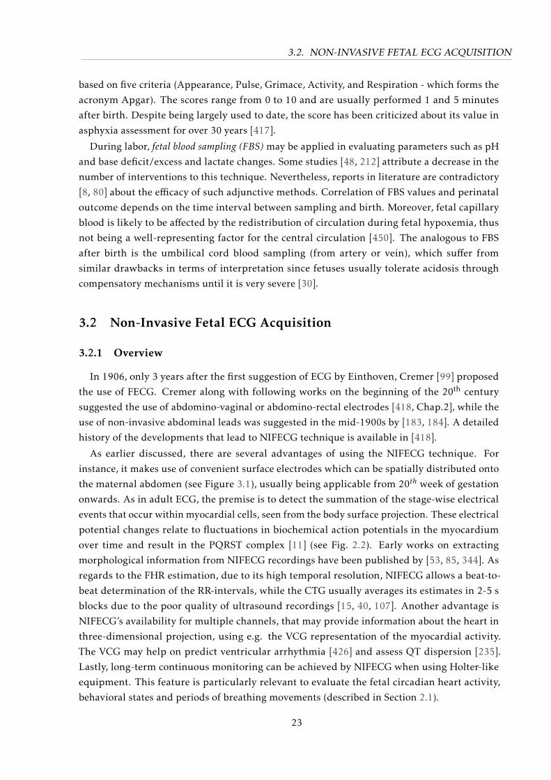
3.2. NON-INVASIVE FETAL ECG ACQUISITION
based on five criteria (Appearance, Pulse, Grimace, Activity, and Respiration - which forms the
acronym Apgar). The scores range from 0 to 10 and are usually performed 1 and 5 minutes
after birth. Despite being largely used to date, the score has been criticized about its value in
asphyxia assessment for over 30 years [417].
During labor, fetal blood sampling (FBS) may be applied in evaluating parameters such as pH
and base deficit/excess and lactate changes. Some studies [48, 212] attribute a decrease in the
number of interventions to this technique. Nevertheless, reports in literature are contradictory
[8, 80] about the efficacy of such adjunctive methods. Correlation of FBS values and perinatal
outcome depends on the time interval between sampling and birth. Moreover, fetal capillary
blood is likely to be affected by the redistribution of circulation during fetal hypoxemia, thus
not being a well-representing factor for the central circulation [450]. The analogous to FBS
after birth is the umbilical cord blood sampling (from artery or vein), which suffer from
similar drawbacks in terms of interpretation since fetuses usually tolerate acidosis through
compensatory mechanisms until it is very severe [30].
3.2 Non-Invasive Fetal ECG Acquisition
3.2.1 Overview
In 1906, only 3 years after the first suggestion of ECG by Einthoven, Cremer [99] proposed
the use of FECG. Cremer along with following works on the beginning of the 20th century
suggested the use of abdomino-vaginal or abdomino-rectal electrodes [418, Chap.2], while the
use of non-invasive abdominal leads was suggested in the mid-1900s by [183, 184]. A detailed
history of the developments that lead to NIFECG technique is available in [418].
As earlier discussed, there are several advantages of using the NIFECG technique. For
instance, it makes use of convenient surface electrodes which can be spatially distributed onto
the maternal abdomen (see Figure 3.1), usually being applicable from 20th week of gestation
onwards. As in adult ECG, the premise is to detect the summation of the stage-wise electrical
events that occur within myocardial cells, seen from the body surface projection. These electrical
potential changes relate to fluctuations in biochemical action potentials in the myocardium
over time and result in the PQRST complex [11] (see Fig. 2.2). Early works on extracting
morphological information from NIFECG recordings have been published by [53, 85, 344]. As
regards to the FHR estimation, due to its high temporal resolution, NIFECG allows a beat-to-
beat determination of the RR-intervals, while the CTG usually averages its estimates in 2-5 s
blocks due to the poor quality of ultrasound recordings [15, 40, 107]. Another advantage is
NIFECG’s availability for multiple channels, that may provide information about the heart in
three-dimensional projection, using e.g. the VCG representation of the myocardial activity.
The VCG may help on predict ventricular arrhythmia [426] and assess QT dispersion [235].
Lastly, long-term continuous monitoring can be achieved by NIFECG when using Holter-like
equipment. This feature is particularly relevant to evaluate the fetal circadian heart activity,
behavioral states and periods of breathing movements (described in Section 2.1).
23
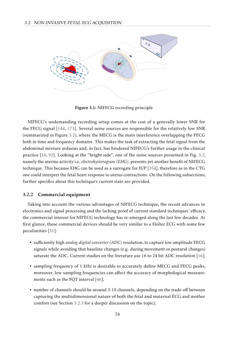
3.2. NON-INVASIVE FETAL ECG ACQUISITION
Figure 3.1: NIFECG recording principle
NIFECG’s undemanding recording setup comes at the cost of a generally lower SNR for
the FECG signal [144, 173]. Several noise sources are responsible for the relatively low SNR
(summarized in Figure 3.2), where the MECG is the main interference overlapping the FECG
both in time and frequency domains. This makes the task of extracting the fetal signal from the
abdominal mixture arduous and, in fact, has hindered NIFECG’s further usage in the clinical
practice [18, 92]. Looking at the “bright side”, one of the noise sources presented in Fig. 3.2,
namely the uterine activity i.e. electrohysterogram (EHG), presents yet another benefit of NIFECG
technique. This because EHG can be used as a surrogate for IUP [354], therefore as in the CTG
one could interpret the fetal heart response to uterus contractions. On the following subsections,
further specifics about this technique’s current state are provided.
3.2.2 Commercial equipment
Taking into account the various advantages of NIFECG technique, the recent advances in
electronics and signal processing and the lacking proof of current standard techniques’ efficacy,
the commercial interest for NIFECG technology has re-emerged along the last few decades. At
first glance, these commercial devices should be very similar to a Holter ECG with some few
peculiarities [51]:
• sufficiently high analog-digital converter (ADC) resolution, to capture low amplitude FECG
signals while avoiding that baseline changes (e.g. during movement or postural changes)
saturate the ADC. Current studies on the literature use 16 to 24 bit ADC resolution [16];
• sampling frequency of 1 kHz is desirable to accurately define MECG and FECG peaks,
moreover, low sampling frequencies can affect the accuracy of morphological measure-
ments such as the FQT interval [46];
• number of channels should be around 3-10 channels, depending on the trade-off between
capturing the multidimensional nature of both the fetal and maternal ECG and mother
comfort (see Section 3.2.3 for a deeper discussion on the topic);
24

3.2. NON-INVASIVE FETAL ECG ACQUISITION
MaternalMuscular Activity(EMG and EHG)
BaselineDrift
(artefacts /respiration)
MaternalECG
(MECG)
PowerlineInterference(50/60 Hz)
Ambient Noise(electromagnetic
radiation)
Noise in ElectronicEquipments(amplifiers)
Electrodecontact noise
(pop / contact)
Motion Artifact(change in impedance)
AbdominalSignal
FetalECG
(FECG)
Figure 3.2: Predominant sources present in abdECG measurements. Interferences with bio-logical origins (on the left), noises originated on interfaces between mother and equipment(below and in the middle), and equipment noise (on the right). Maternal ECG is the mostsignificant disturbance. Modified from [16].
• battery life should be able to cover 24-48 h of recordings so that the feto-maternal circadian
rhythm and fetal behavioral states (presented in Section 2.1.6) can be observed.
Currently, only two commercial NIFECG monitoring equipment are available, both having
obtained FDA 510(k) clearance for intrapartum period (WOG > 36 weeks), namely AN24/Novii
from Monica Healthcare (Nottingham, UK) and M100/M1000 monitors from MindChild Medi-
cal (North Andover/MA, USA).
Monica’s AN24 was the first available apparatus which has been commercialized in Europe
(CE approval) for nearly 10 years. Despite being recommended for WOG≥36 weeks, in Europe,
its use is allowed for earlier WOGs (≥20 weeks). Monica provides the FHR, maternal heartrate (MHR) and uterine activity (EHG) in real-time with information on three leads and has
shown some initial fair results. However, studies using the AN24 are still limited in population
size and heterogeneity. Besides, Monica depends on the patient’s abdomen receiving thorough
skin preparation with a special abrading solution and gentle scrub of the skin for a better signal
quality, which may be an inconvenience [16, 466].
Meridian monitors use a 32 lead system [51] where no skin preparation is required [466],
however, its use is still restricted, and little information is available about its design and
characteristics. Furthermore, very few studies are available since it has obtained FDA(k) for
intrapartum monitoring on 2012.
Aside from the described commercial equipment, a handful of other companies, such as
Nemo Healthcare (Eindhoven, Netherlands), PregSense from Nuvo Group (Tel Aviv, Israel) and
KOMPOREL from the Institute of Technical and Medical Equipments (ITAM) (Zabrze, Poland),
25
3.2. NON-INVASIVE FETAL ECG ACQUISITION
have shown their intention of releasing novel NIFECG monitors in the near future. However,
when applying commercial instruments in research there is the disadvantage of not knowing
exactly what is inside the architecture and how the signal extraction is precisely performed.
These cons can lead to unwitting mistakes and do not permit a full analysis of the data. All
in all, commercial applications of NIFECG monitoring are in their early days, and there is a
growing interest in improving their performance, aiming to reach a point where they provide
actionable information to clinicians.
3.2.3 Electrode configurations
Aside from the ADC used, when attempting to collect NIFECG data careful consideration
has to be given to the electrode configuration applied. To date, there is no available standard
for the positioning of abdominal electrodes in NIFECG recordings. Similarly to adult electro-
cardiography, the morphology of the cardiac signal strongly depends on the lead configuration
employed. In the abdECG case, although the lead system may be chosen and kept relatively
constant (depending of course on the maternal and girth’s size), the fetal position is time-
varying, individual-dependent and cannot be easily identified prior to electrode placement. A
general-purpose optimal electrode placement is impracticable for this reason [4].
Before proceeding, the terminology used in this work is defined based on the recommen-
dations of the American Heart Association (AHA) [231]. Bioamplifiers usually make use of
differential amplifiers, thus there are two main electrical potential inputs (V +in and V −in). As
input to the amplifier, one generally has two active electrode, one connected to the positive
terminal (V +in, henceforth graphically shown as + ) and another on the negative terminal (V −in,
depicted as - ). In addition, a reference electrode (here termed as ground electrode – “GND”)
is used to improve common mode (unwanted noise) rejection. Take for instance Einthoven’s
lead II, the positive, negative, and ground electrodes are located on the left leg, right arm, and
right leg, respectively. The negative electrode can physically exist (as in Einthoven’s lead II) or
be calculated as the average of some (or all) leads, as in Wilson’s central terminal. When this
electrode physically exists, the derivation is often referred to as “bipolar”, when otherwise it
is referred as “unipolar”. However, the use of this historical nomenclature (i.e. “bipolar” and
“unipolar”) is discouraged by the AHA since all leads are effectively bipolar, thus, the term
“unipolar” is described as lacking precision [231].
Numerous configurations have been proposed in the literature in an attempt to standardize
the recording procedure. Several of those configurations are presented in Figure 3.3. From
Fig. 3.3 it is evident that some authors rely on the most common fetal presentation (i.e. vertex,
breech or shoulder), in order to reduce the number of leads used by aiming at usual positions
for fetal head/thorax and, consequently, minimizing the application’s complexity. Meanwhile,
other authors aim at covering most of the abdomen to maximize the chances of obtaining FECG
signal [4]. The inter-electrode distance also plays an important role in the signal SNR, FECG
and MECG power. The closer the electrodes are from one another in a differential scheme, the
more local similar information is collected on both electrodes. As a consequence, the MECG
26
3.2. NON-INVASIVE FETAL ECG ACQUISITION
power is generally smaller, while FECG, and electromyogram (EMG) noise (muscle crosstalk)
have a higher power.
Despite the various electrode configurations proposed, to date very few studies have compared
the different options that exist. Rooijakkers et al. [354] is one exception, in which both negative
and ground electrodes placed on the patient’s right side (as depicted in Fig. 3.3 d). Rooijakkers
et al. [354] evaluated the effect of increasing the distance between electrodes, considering the
SNRs of maternal and fetal ECGs as well as EHG as goodness criteria. The authors suggested
two differential lead schemes, one with 5 electrodes for intrapartum recordings (inter-electrode
distance of 16 cm - similar to figure 3.3a with an additional central electrode) and a 6 electrodes
scheme for preterm recordings (distance 20 cm - similar to Figure 3.3d). Such configurations
should optimally record the MECG, FECG, and uterine activity. Despite the interesting analysis,
this clinical study was limited to 5 patients, each recording having 20 min in duration and
performed at high gestational weeks (> 39 weeks). Moreover, the proposed lead configuration
was very restrictive with a single triangular configuration and negative electrode kept in the
same position. Another study, which considered signal quality throughout different channels
was performed by Clifford et al. [85, 89]. The authors described an “over-complete” set of
electrodes (see Fig. 3.3 j) and mentioned that some channels, at a particular time instant,
contributed most to the quality of the FECG signals. However, the authors noted that the signal
quality varies across patients (and time), thus an automatic selection of channels based on signal
quality measures is necessary [51]. Lastly, the optimal number of electrodes may depend on
the extraction method used. For instance, extraction routines may require from one to several
abdominal leads, meanwhile, other methods need one (or more) MECG chest leads. Further
details about these signal processing requirements are discussed in Section 3.3.1.
While designing electrode configurations for portable equipment, it should be kept in mind
that an increasing number of electrodes is responsible for higher power consumption and
decrease in patient comfort. The same applies for MECG leads, which despite being conve-
nient for distinguishing between maternal from fetal ECG signals, they increase the hardware
requirements and add extra leads outside the abdominal area that may be less comfortable.
Another consideration is the location of the negative and common ground electrodes. For
NIFECG applications, a ground electrode is recommended, since it reduces the common mode
interference while enhancing the relative contribution of the signals of interest [164, 268, 354].
3.2.4 Available NIFECG databases
The increasing interest in the NIFECG created the need for data platforms where researchers
could compare their extraction/detection results. Few freely available databases emerged over
the last two decades, which are summarized below [49, 51, 365]:
DAISY database [109, 288] consists of a single 10 seconds recording using eight ECG channels
(5 abdominal and 3 thoracic leads) sampled at 250 Hz. The study was performed by the
Department of Electrical Engineering of the Katholieke Universiteit Leuven (Belgium).
The dataset is available at http://homes.esat.kuleuven.be/~smc/daisy/.
27
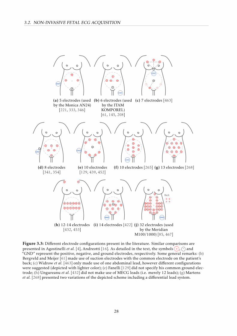
3.2. NON-INVASIVE FETAL ECG ACQUISITION
GND
(a) 5 electrodes (usedby the Monica AN24)
[221, 333, 346]
GND
(b) 6 electrodes (usedby the ITAMKOMPOREL)[61, 145, 208]
GND
(c) 7 electrodes [463]
GND
(d) 8 electrodes[341, 354]
GND
(e) 10 electrodes[129, 439, 452]
GND
(f) 10 electrodes [265] (g) 13 electrodes [268]
(h) 12-14 electrodes[432, 453]
GND
(i) 14 electrodes [422]
GND
Back
(j) 32 electrodes (usedby the Meridian
M100/1000) [85, 467]
Figure 3.3: Different electrode configurations present in the literature. Similar comparisons arepresented in Agostinelli et al. [4], Andreotti [16]. As detailed in the text, the symbols + , - and“GND” represent the positive, negative, and ground electrodes, respectively. Some general remarks: (b)Bergveld and Meijer [61] made use of suction electrodes with the common electrode on the patient’sback; (c) Widrow et al. [463] only made use of one abdominal lead, however different configurationswere suggested (depicted with lighter color); (e) Fanelli [129] did not specify his common ground elec-trode; (h) Ungureanu et al. [432] did not make use of MECG leads (i.e. merely 12 leads); (g) Martenset al. [268] presented two variations of the depicted scheme including a differential lead system.
28

3.2. NON-INVASIVE FETAL ECG ACQUISITION
Non-Invasive Fetal Electrocardiogram Database [161] comprises
55 multichannel (2 thoracic and 3-4 abdominal leads) recordings taken from a single
woman between the 21st and 40th WOG. Recordings were performed using a g.BSamp
Biosignal Amplifier (GTech GmbH, Austria) at 1 kHz, with 16-bit resolution, bandpass
filtered around 0.01-100 Hz and using a notch filter at 50 Hz. Recordings widely vary
in duration ranging from less than 2 min segments up to 46 min, however, no reference
annotation was provided. The data has been prepared by the Digital Signal Processing
Group of the Electronics Engineering Department at the University of Valencia (Spain)
and is available on Physionet [161] (https://physionet.org/physiobank/database/
nifecgdb/).
Abdominal and Direct Fetal Electrocardiogram Database [208] consists of five, 5-minute, mul-
tichannel (4 abdominal and one scalp ECG channels) recordings of women in labor (38th
to 41st WOG). The electrode configuration consisted of four electrodes placed around the
navel, a reference electrode placed above the pubic symphysis and a common mode elec-
trode placed on the left leg. Recording were performed using the KOMPOREL (mentioned
in Section 3.2.2) that has 16-bit resolution, 1 kHz sampling rate, bandwidth 1-150 Hz
and digital filters for removing baseline and power-line interference. Reference FQRS
annotation was derived from the FSE recording. The recordings were acquired in the
Department of Obstetrics at the Medical University of Silesia (Poland) and are available
on Physionet [161] (https://physionet.org/physiobank/database/adfecgdb/).
Physionet/Computing in Cardiology Challenge 2013 Database [92, 395] is a compilation from
five different databases [54, 395]: the two previous datasets, Scalp FECG Database (pri-
vate), Ukraine Non-Invasive FECG (private) and simulated data (further described). The
database includes 447 min of data, with up to 4 channels, resampled at 1 kHz. This
is the largest publicly available FECG dataset to date, available on Physionet [161]
(http://www.physionet.org/challenge/2013/). The database was used as training set
for the PCINC 2013.
However, the present databases are still very limited in: i) number and duration of the
recordings; ii) variety of WOG; iii) information on the subject’s pathophysiological background;
iv) expert’s annotations of the FQRS locations v) events such as fetal movement and presence
of ectopic beats; vi) silver-standard for FECG morphology. Hence, there is a demand for a
more complete database, which may allow FHR, FHRV and morphological analysis of the FECG.
Some further specifics on such idealistic database are described in [49, 51, 54].
3.2.5 Validity and usability of the non-invasive fetal ECG
As previously shown, NIFECG can be used for two major types of analysis, namely FHR/FHRV
and the morphological analysis of the extracted FECG waveform. Regarding gold-standards for
the afore mentioned metrics, FHR/FHR can be compared with CTG (antepartum/intrapartum,
29
3.2. NON-INVASIVE FETAL ECG ACQUISITION
less accurate) and FSE (intrapartum, accurate), while for FECG morphology requires either
FMCG (antepartum1) or FSE (intrapartum) as reference.
Although the Monica AN24 has not yet gained a significant foothold in the monitoring
market, several studies and commercial NI-FECG equipment claim to obtain accurate FHR
tracings [51, 466]. For instance, Reinhard et al. [346] has found that the NIFECG and CTG
characterize FHR trace in a similar manner with regards to acceleration count, decelerations
count and coincidence, variability and baseline for n = 27 subjects. Moreover, the author found
an overall strong correlation (Pearson’s r = 0.91) between the techniques’ FHR traces. Similar
results were obtained by a more recent study by [228], on which moderate to high correlations
(r = 0.57− 0.97) were found n = 39 recordings of 20 min duration including 2 min of auditory
stimulus. Another important aspect addressed by [407] was the lower rate of confusion between
maternal HR and FHR achieved by NIFECG, when compared with CTG. High accuracy has
also been reported in the literature when comparing FSE and NIFECG specially when using the
open-source databases that counted with FSE for FQRS gold-standard.
With regards to the morphology of the signal, in Clifford et al. [85], the authors recorded
the NIFECG on n = 32 term laboring women who had FSE placed after clinical indication.
They evaluated the accuracy of the FST segment extracted on the NIFECG (by an automated
algorithm) against the reference FST segment extracted from the FSE (using the same automated
algorithm). The root mean square error between the FST calculated by both modalities averaged
over all processed segments was 3.2%, indicating that accurate extraction of the FST segment
from the NIFECG may be feasible. Similarly, [344] investigated the feasibility of NIFECG FST
analysis by comparing the AN24 and STAN on n = 6 pregnant women during birth. Non-invasive
FST was possible in 50 % the cases due to absence of fetal T-wave. Furthermore, McDonnell et al.[274] has found a very low difference between T/R ratios obtained by STAN and the Meridian
monitor for n = 27 term laboring women. Lastly, in Behar et al. [56] the authors showed the
possibility to recover the FQT from the NIFECG from n = 22 term women. The study made use
of manually annotated FQT on both NIFECG and FSE, which were fused prior to comparison.
The errors found between NIFECG and FSE FQT were in the range of QT annotations performed
on adult ECGs [51]. All these studies are very encouraging, nevertheless a careful reader should
have concerns about the reference being provided by a single cephalic lead and how the effect
of the electrode positioning may affect the final results for NIFECG technique. Since the current
studies are fairly limited in number, such conclusions should be considered with caution.
Considering the quality of such recordings, as early as 1995 Crowe et al. [100] have qualita-
tively shown the benefits and challenges in long-term NIFECG monitoring, due to the lower
SNR of the fetal signal. Taylor et al. [423] reported being able to visually inspect FECG sig-
nal (including P, QRS and T waves) in 80 % for this study’s population (15 pregnant women,
24-41 WOG, half of which with ≥ 39 weeks) using 15 min recordings. Pieri et al. [333] made
use of 400 short-term recordings (5-10 min) at different stages and pregnancy, using a FHR
obtainal success rate the authors produced trends for signal quality throughout pregnancy.
1 Please note that there is a fundamental complication in using both NIFECG and FMCG simultaneously, due to theelectromagnetic interference that the techniques have on each other.
30
3.2. NON-INVASIVE FETAL ECG ACQUISITION
Although little information on the subjects pathophysiological states is revealed, it is clear that
around the 28th WOG NIFECG’s quality is expressively reduced. Fuchs et al. [145], who used
the KOMPOREL, investigated pregnant women ranging between 28 and 42 WOG and have
found no correlation between the percentage of signal loss and gestational age, nor between
signal loss and BMI. A more comprehensive study using the AN24 by Graatsma et al. [163]
evaluated long-term 15 h recordings of 150 preterm pregnant and 1-hour recordings of 22
laboring women, who had FSE simultaneously applied. Regarding the quality of recordings, the
authors have found that 82 % the long-term recordings were of good quality (i.e. where on 60 %
of the time FECG signal was present – as defined by the authors). The study also suggests that
during the night period signal quality increased. According to the authors, a strong and signif-
icant correlation between FSE and NIFECG’s FHR (r = 0.99) and FHRV short-term variability
[106] (r = 0.79) were found during labor. Analogously, Reinhard et al. [345] assessed the signal
quality of the FHR estimated from n = 144 NIFECG and CTG recordings during the first and
second stages of labor. The study showed significant better results for NIFECG during the first
stage, while no difference in signal loss was found during the second stage. Associated to these
results, both Graatsma et al. [163], Van Laar et al. [439] have found no significant effect of BMI
on NIFECG recording quality, however Van Leeuwen et al. [446] showed an increase in signal
loss due to obesity.
Aside from the few publications herein listed and a handful of others provided by the current
NIFECG commercial equipment, there is not much evidence on the ability of these devices to
extract and detect fetal signals. For instance, neither Monica’s nor Meridian have published
any large randomized trial to compare NIFECG recordings with other gold-standards such as
CTG and FSE. Nor have they demonstrated NIFECG’s ability to improve neonatal outcome.
Moreover, little is known about the quality of NIFECG recordings, particularly on earlier WOG
(i.e. WOG < 28). This latter analysis is important to figure out what factors aside from the vernix
caseosa can influence the quality of NIFECG recordings, which would enable the technique to be
used in a broader number of patients. Moreover, as previously describe, a study on FHRV is only
complete if additional information about the fetal behavioral state, time of day and activity (i.e.
fetal movement) is available. Similarly, to be able to analyze the FECG morphology, information
about the observed projection (i.e. electrode positioning) is required. Such information could be
partially obtained by obtaining a VCG representation of fetal heart, as suggested by [452].
In any manner, the fetal signal component in the NIFECG should be reliably extracted and
detected before any further clinical analysis take place. Due to the more fundamental data
collection and signal processing problems that are involved in NIFECG technique, the clinical
analysis of the parameters that could be obtained through these recordings (i.e. FHR, FHRV
and morphological analysis) are out of the scope of this thesis.
31

3.3. NON-INVASIVE FETAL ECG EXTRACTION METHODS
3.3 Non-Invasive Fetal ECG Extraction Methods
Before proceeding, the mathematical notation adopted in the following sections (common
in estimation theory) is summarized in Table 3.2. When looking for any other variable, please
refer to the List of Symbols.
Table 3.2: Notation used in this work.
Notation Represents Font characteristicsx regular font scalar
xk , x[n]subscripted index/square brackets discrete-time variable x at time k/n
x(t) parenthesis signal at continuous time tx underlined vectorA capitalized, boldfaced matrixx overlined meanx hat estimate for variable xx tilde estimation error for x, i.e. x − xA capitalized, tilde linearized/approximate matrix
xk|k−1 subscripted index† a priori estimate of xk conditioned to allprior measurements except at time k
xk|k subscripted index‡ a posteriori estimate of xk conditionedto all measurements up to time k
† Also often described in literature as x−k . The notation in this work is adopted from Sayed [379].‡ Also often described in literature as x+
k .
3.3.1 Overview on the non-invasive fetal ECG extraction methods
One of the major challenges in FECG analysis is separating the fetal signal from its surround-
ing noise. This section gives an overview on the current solutions to the problem. Particular
focus is given to the Kalman Filter (KF) algorithm, due to its versatile and mathematically sound
framework. For further information on these signal processing techniques, the reader is referred
to the following reviews [51, 92, 173, 365, 418].
Extraction techniques aim at estimating the fetal signal either directly from abdominal
signals or indirectly by first estimating the MECG and then treating the signal residuals as
FECG and noise. The first (i.e. direct FECG estimation) is usually unfeasible due to various noise
signals involved which makes the source separation problem more complex. Therefore, most
approaches available in the literature are indirect. In the following sections, a brief description
of the most important algorithms is presented (see Fig. 3.4). These methods can be categorized
in: Adaptive Methods, Template Subtraction, Blind Source Separation or combination of those
(i.e. Hybrid Methods). Since the Physionet/Computing in Cardiology Challenge (PCINC) 2013
[92, 395] enabled a direct benchmark between some of these methods, exemplary applications
are mentioned while describing each category.
32
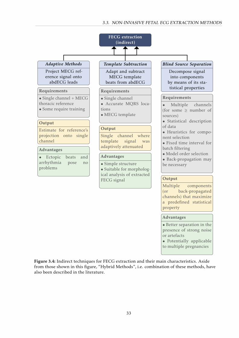
3.3. NON-INVASIVE FETAL ECG EXTRACTION METHODS
FECG extraction(indirect)
Blind Source Separation
Decompose signalinto components
by means of its sta-tistical properties
Template Subtraction
Adapt and subtractMECG template
beats from abdECG
Adaptive Methods
Project MECG ref-erence signal onto
abdECG leads
Requirements
• Single channel + MECGthoracic reference• Some require training
Output
Estimate for reference’sprojection onto singlechannel
Advantages
• Ectopic beats andarrhythmia pose noproblems
Requirements
• Multiple channels(for some ≥ number ofsources)• Statistical descriptionof data• Heuristics for compo-nent selection• Fixed time interval forbatch filtering•Model order selection• Back-propagation maybe necessary
Output
Multiple components(or back-propagatedchannels) that maximizea predefined statisticalproperty
Advantages
• Better separation in thepresence of strong noiseor artefacts• Potentially applicableto multiple pregnancies
Requirements
• Single channel• Accurate MQRS loca-tions•MECG template
Output
Single channel wheretemplate signal wasadaptively attenuated
Advantages
• Simple structure• Suitable for morpholog-ical analysis of extractedFECG signal
Figure 3.4: Indirect techniques for FECG extraction and their main characteristics. Asidefrom those shown in this figure, “Hybrid Methods”, i.e. combination of these methods, havealso been described in the literature.
33
3.3. NON-INVASIVE FETAL ECG EXTRACTION METHODS
Adaptive methods
As the FECG overlaps in time and frequency with its surrounding noise, especially with
the MECG, simple linear filters with fixed coefficients (i.e. constant transfer function) are not
able of separating the FECG from NI-FECG recordings [173]. Adaptive Methods (AM) are more
sophisticated approaches that attempt to project one (or more) MECG reference lead(s) onto
each abdominal lead, hence estimating the projection of the maternal signal on the abdECG
channels. This is obtained by continuously adapting AM’s filter coefficients while following
the MECG reference. In the literature, some authors refer to such structure as Adaptive NoiseCanceller (ANC) [463]. Exemplary AM methods are the Least Mean Squares (LMS) [463], RecursiveLeast Squares (RLS) and Echo State Network (ESN) [200]. According to Behar et al. [52], the LMS
attempts to minimize the mean square error (MSE) between reference MECG and abdominal
signal, regarding solely the information on the current and previous samples. Similarly, the
RLS minimizes the sum of squared errors using all available samples of the measured signal.
For this filter, a forgetting factor is required for weighting down the past error’s influence
while calculating the current filter weight. Both LMS and RLS assume linear propagation of
the MECG signal throughout the body. Unlike the previously described methods, the ESN is
capable of nonlinear projecting the MECG onto abdominal channels, achieving better FECG
estimates [18, 52]. However, ESN entails a neural network approach that comes at cost of a
much higher computational load. A more extensive review on AM for FECG can be found in
Behar et al. [52]. Several alternative methods, both linear and nonlinear, have been proposed
for the purpose of extracting the FECG, e.g. using Wiener filtering [352, 387] or adaptive
finite impulse response (FIR) schemes e.g. [34, 35, 76, 257, 390, 412]. Due to the lack of MECG
reference leads, AM were not preferred during the PCINC 2013, one exception was Rodrigues
[352], who obtained poor results by making use of the Wiener filter to follow 3 out of the 4
available abdominal leads. Some of the drawbacks from AM are: i) the stringent necessity
of a reference lead, which adds complexity and potential discomfort to recording system,
and ii) the fact that some of those methods e.g. ESN and Adaptive Neuro-Fuzzy InterferenceSystem (ANFIS) [35] are based on neural networks, therefore require a training phase which can
increase computational/time cost.
Template subtraction methods
Template Subtraction (TS) methods make use of the maternal signal pseudo-periodicity in
obtaining a mean MECG cycle (so-called “template”), i.e. coherent averaging [353] maternal
beats [267]. This procedure heavily depends on accurate maternal QRS (MQRS) detections. Next,
the template is adapted onto the abdECG on a beat-to-beat basis, therefore estimating the MECG
on each channel. Last, the estimated MECG signal is subtracted from the abdECG channel,
leaving behind FECG signal and noise as residuals. In order to account for varying morphologies
of the MECG, this average template is usually built on every couple seconds/minutes or updated
online. TS algorithms impose the fewest number of restrictions on the recording system and
can be applied on a single lead. A variety of TS techniques have been described in the literature
34
3.3. NON-INVASIVE FETAL ECG EXTRACTION METHODS
[20, 54, 78, 113, 254, 268, 430, 433, 454, 477]. For instance, the T Sc [78, 111, 434] simply adapts
each beat using a single scalar gain [54]. This approach was used in early works at the IBMT
in the field of FECG [16, 477]. Analogous procedures were applied during the PCINC 2013 by
[54, 337]. More elaborate techniques such as the T Sm [268] make use of different scalar gains
for each P-QRS-T waveform. Template adaptation (T Sa) [20, 179] enables width and height
adaption of the template on a sample-basis, using concepts of Self-Organizing Maps (SOMs).Ungureanu et al. [433], Vullings et al. [454] suggested the use of linear prediction for individually
weighting previous maternal cycles, here called T Slp. Sameni et al. [368, 369, 370] proposed
the use of a TS technique based on the EKF, namely T Sekf . Differently from the previously
described methods, T Sekf performs a continuous and adaptive sample-by-sample estimation
of the MECG and, consequently, the FECG and noise contained in the residual. As compared
with the other approaches, T Sekf framework is more adaptive, theoretically allowing better
estimation of the MECG in highly non-stationary scenarios [18]. TS are usually straightforward
techniques, that imply the least distortions on the estimated FECG as shown in [18].
Blind source separation
Differently from AM and TS, Blind Source Separation (BSS) methods strive to decompose
the multichannel abdominal mixture into different components without a priori knowledge
about the signal itself. In fact, BSS attempts to separate the sources present in the abdECG
(i.e. FECG, MECG and noise/artefacts) according to their statistical properties, e.g. correlation
or independence. Exemplary BSS algorithms are the Principal Component Analysis (PCA) [42,
308], Independent Component Analysis (ICA) [109, 447, 474, 475], Singular Value Decomposition(SVD) [75, 219], Gaussian Processes (GP) [301, 350], Tensors Decomposition (TD) [301–303]
and Nonlinear State-Space Projection (NSSP) [236, 348, 387]. In case additional information is
provided (e.g. MQRS locations) methods are referred to as semi-BSS, e.g. the Periodic ComponentAnalysis (πCA) [366]. For consistency, BSS extraction techniques using ICA, PCA and etc. are
further referred to as BSSica, BSSpca, etc., respectively.
Some early works on BSS techniques for solving the NIFECG problem have been published
[42, 109, 474] and revisited during the PCINC 2013 [54, 447]. BSS techniques generally process
segments of signal, within this segment the mixture between sources is assumed to be stationary,
i.e. the statistical properties of the signal do not vary over time. This assumption was shown
in Andreotti et al. [18] to be a dangerous assumption. Moreover, these algorithms usually2
require multiple abdominal (and/or thoracic) leads, BSSica in particular, requires as input
at least the same number of leads as sources [221]. Additionally, some BSS methods suffer
from scaling (e.g. BSSpca) and permutation indeterminacy3 (e.g. BSSica). Furthermore, the
2 Some works have described SVD-based approaches for single-lead applications [37, 219, 304]3 Component selection constitutes the major challenge concerning BSS techniques [18]. Selecting one or more
components that well represent the MECG is as-is difficult, making a distinction between MECG and FECG andcorrectly selecting the FECG signal (for a direct approach) is nearly impossible. Particularly for ICA, permutationindeterminacy is a well know problem, where the positioning of independent component (IC)s inside ICA’s outputis a priori unknown. This problem makes the already cumbersome task of automatic selection of the IC(s) ofinterest (i.e. MECG/FECG) more complex [20, 83, 459].
35
3.3. NON-INVASIVE FETAL ECG EXTRACTION METHODS
issue of determining the optimal number of underlying sources, referred to as model order
selection problem [201, 327], should be addressed. The problem states that an inappropriate
choice/estimation of the number of components may lead to unsatisfactory source separation.
In order to partially overcome this difficulty, a PCA dimension reduction step is usually applied
[197]. Lastly, the length of the evaluated signal segment has to be considered. The longer the
segment, the more critical the assumption of stationarity becomes. For lengthy segments, BSS
techniques are expected to underperform; meanwhile, if this segment is too short, there may not
be sufficient statistical information to represent MECG/FECG’s features (e.g. non-Gaussianity),
therefore also preventing a satisfactory source separation. Nevertheless, if those technique’s
assumptions are respected and parameters/heuristics well-designed, accurate FQRS results can
be achieved. Regarding morphological analysis, Andreotti et al. [18] has shown that it should be
performed in the observational domain, rather than source domain. Unlike AM and TS, BSS
techniques are usually applied in batches4 of signal.
Hybrid extraction methods
Aside from the aforementioned techniques, extraction routines may also be composed by
combining methods from different subgroups (shown in Fig. 3.4). One example is the deflation
procedure introduced by Sameni et al. [367]. This general procedure transforms multichannel
abdominal signals into the source-domain (by means of any BSS method); next the MECG
interference is removed from the source-domain components by means of TS techniques; and,
at last, the denoised sources are back-propagated to the observational domain. This procedure
is repeated a number of times until the output signals satisfy some predefined measure of
signal separability [367]. Sameni et al. [367] themselves applied the framework in NI-FECG
extraction using BSSπCA [366] and T Sekf combination, as did [170] during the PCINC 2013,
while [303] combined TD and BSS techniques. Another example of hybrid method is the T Spca[18, 54, 219] which, in essence, is a TS method that decomposes stacked maternal cycles using
PCA. T Spca selects a couple first principal components, next a back-propagation step takes
place on a beat-to-beat basis, producing MECG estimates for every maternal cycle. T Spca was
applied during the PCINC 2013 by [54, 254]. Table 3.3 summarizes the different extraction
methods mentioned throughout the present section as in [51].
3.3.2 Kalman filtering basics
In the previous section, the strengths and weaknesses of three different classes of extraction
methods were delineated. When contemplating real world applications, a reduced number of
electrodes is desirable for improving subject’s comfort and allowing its use in an ambulatory
environment. As mentioned in Sections 3.2.3 and 3.3.1, selecting applicable extraction methods
is highly dependent on the available electrode configuration. TS techniques impose the fewest
4 Please notice that every category of method requires some initialization procedure, after this period TS and AMcan run only e.g. TS initializes its templates and can adapt it on-the-go. BSS techniques, on the other hand, requirea chunk of data which should be long (e.g. 1 min long) and spatially complete (e.g. 8 channels) to enable theextraction of the desired components.
36
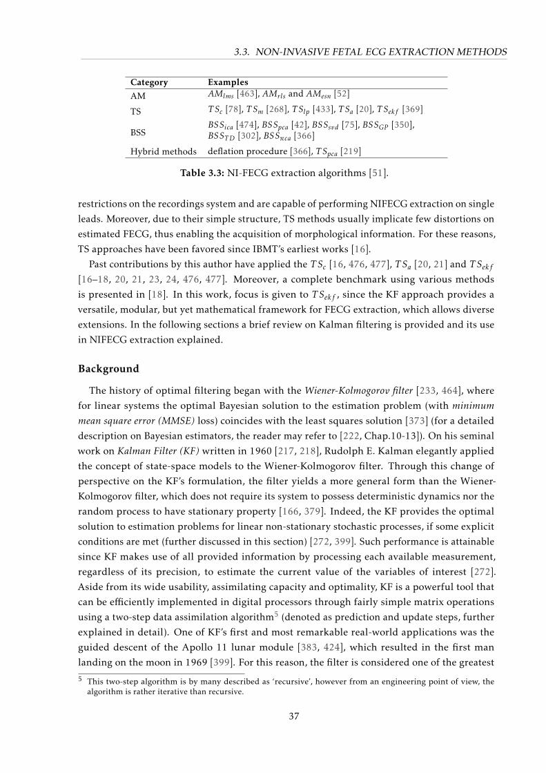
3.3. NON-INVASIVE FETAL ECG EXTRACTION METHODS
Category Examples
AM AMlms [463], AMrls and AMesn [52]
TS T Sc [78], T Sm [268], T Slp [433], T Sa [20], T Sekf [369]
BSSBSSica [474], BSSpca [42], BSSsvd [75], BSSGP [350],BSSTD [302], BSSπca [366]
Hybrid methods deflation procedure [366], T Spca [219]
Table 3.3: NI-FECG extraction algorithms [51].
restrictions on the recordings system and are capable of performing NIFECG extraction on single
leads. Moreover, due to their simple structure, TS methods usually implicate few distortions on
estimated FECG, thus enabling the acquisition of morphological information. For these reasons,
TS approaches have been favored since IBMT’s earliest works [16].
Past contributions by this author have applied the T Sc [16, 476, 477], T Sa [20, 21] and T Sekf[16–18, 20, 21, 23, 24, 476, 477]. Moreover, a complete benchmark using various methods
is presented in [18]. In this work, focus is given to T Sekf , since the KF approach provides a
versatile, modular, but yet mathematical framework for FECG extraction, which allows diverse
extensions. In the following sections a brief review on Kalman filtering is provided and its use
in NIFECG extraction explained.
Background
The history of optimal filtering began with the Wiener-Kolmogorov filter [233, 464], where
for linear systems the optimal Bayesian solution to the estimation problem (with minimummean square error (MMSE) loss) coincides with the least squares solution [373] (for a detailed
description on Bayesian estimators, the reader may refer to [222, Chap.10-13]). On his seminal
work on Kalman Filter (KF) written in 1960 [217, 218], Rudolph E. Kalman elegantly applied
the concept of state-space models to the Wiener-Kolmogorov filter. Through this change of
perspective on the KF’s formulation, the filter yields a more general form than the Wiener-
Kolmogorov filter, which does not require its system to possess deterministic dynamics nor the
random process to have stationary property [166, 379]. Indeed, the KF provides the optimal
solution to estimation problems for linear non-stationary stochastic processes, if some explicit
conditions are met (further discussed in this section) [272, 399]. Such performance is attainable
since KF makes use of all provided information by processing each available measurement,
regardless of its precision, to estimate the current value of the variables of interest [272].
Aside from its wide usability, assimilating capacity and optimality, KF is a powerful tool that
can be efficiently implemented in digital processors through fairly simple matrix operations
using a two-step data assimilation algorithm5 (denoted as prediction and update steps, further
explained in detail). One of KF’s first and most remarkable real-world applications was the
guided descent of the Apollo 11 lunar module [383, 424], which resulted in the first man
landing on the moon in 1969 [399]. For this reason, the filter is considered one of the greatest
5 This two-step algorithm is by many described as ‘recursive’, however from an engineering point of view, thealgorithm is rather iterative than recursive.
37
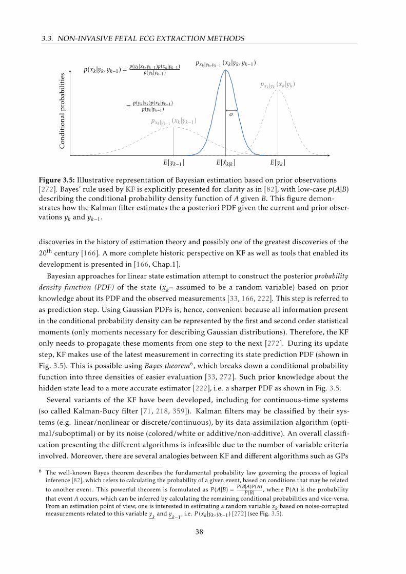
3.3. NON-INVASIVE FETAL ECG EXTRACTION METHODS
pxk |yk−1 (xk |yk−1)
pxk |yk ,yk−1 (xk |yk , yk−1)
pxk |yk (xk |yk)
σ
p(xk |yk , yk−1) = p(yk |xk ,yk−1)p(xk |yk−1)p(yk |yk−1)
= p(yk |xk )p(xk |yk−1)p(yk |yk−1)
E[yk−1] E[xk|k] E[yk]
Con
ditiona
lproba
bilities
Figure 3.5: Illustrative representation of Bayesian estimation based on prior observations[272]. Bayes’ rule used by KF is explicitly presented for clarity as in [82], with low-case p(A|B)describing the conditional probability density function of A given B. This figure demon-strates how the Kalman filter estimates the a posteriori PDF given the current and prior obser-vations yk and yk−1.
discoveries in the history of estimation theory and possibly one of the greatest discoveries of the
20th century [166]. A more complete historic perspective on KF as well as tools that enabled its
development is presented in [166, Chap.1].
Bayesian approaches for linear state estimation attempt to construct the posterior probabilitydensity function (PDF) of the state (xk– assumed to be a random variable) based on prior
knowledge about its PDF and the observed measurements [33, 166, 222]. This step is referred to
as prediction step. Using Gaussian PDFs is, hence, convenient because all information present
in the conditional probability density can be represented by the first and second order statistical
moments (only moments necessary for describing Gaussian distributions). Therefore, the KF
only needs to propagate these moments from one step to the next [272]. During its update
step, KF makes use of the latest measurement in correcting its state prediction PDF (shown in
Fig. 3.5). This is possible using Bayes theorem6, which breaks down a conditional probability
function into three densities of easier evaluation [33, 272]. Such prior knowledge about the
hidden state lead to a more accurate estimator [222], i.e. a sharper PDF as shown in Fig. 3.5.
Several variants of the KF have been developed, including for continuous-time systems
(so called Kalman-Bucy filter [71, 218, 359]). Kalman filters may be classified by their sys-
tems (e.g. linear/nonlinear or discrete/continuous), by its data assimilation algorithm (opti-
mal/suboptimal) or by its noise (colored/white or additive/non-additive). An overall classifi-
cation presenting the different algorithms is infeasible due to the number of variable criteria
involved. Moreover, there are several analogies between KF and different algorithms such as GPs
6 The well-known Bayes theorem describes the fundamental probability law governing the process of logicalinference [82], which refers to calculating the probability of a given event, based on conditions that may be related
to another event. This powerful theorem is formulated as P (A|B) = P (B|A)P (A)P (B) , where P(A) is the probability
that event A occurs, which can be inferred by calculating the remaining conditional probabilities and vice-versa.From an estimation point of view, one is interested in estimating a random variable xk based on noise-corruptedmeasurements related to this variable y
kand y
k−1, i.e. P (xk |yk , yk−1) [272] (see Fig. 3.5).
38
3.3. NON-INVASIVE FETAL ECG EXTRACTION METHODS
[82, 342, 357], hidden Markov model (HMM) [147] and Particle Filters [33]. This work focuses
on the digital implementation of the KF algorithm, therefore its discrete form is used. A brief
derivation is presented based on [70, 222, 245, 272, 362, 379, 399, 424, 461]. Basic concepts in
linear algebra, system theory and probability theory, necessary for the understanding of this
derivation, are explained in [399, Chap.1-3].
A discrete-time linear system can be represented in the state-space form as follows, also
known as canonical representation of the KF model [218]:
xk = Fk−1xk−1 + Gk−1uk−1 +wk−1 , (3.1)
yk
= Hkxk + vk , (3.2)
where k ∈ Z≥0 represents the discrete-time index. xk is the hidden state variable, which we
attempt to estimate from our observations yk
(sensor data). The matrices Fk, Gk and Hk are
considered known matrices. The state transition matrix Fk is responsible for describing the
dynamics of our state, the control input matrix (Gk) determines how a known control input
(uk) influences the system, while the observational matrix (Hk) explains how these states are
observed. The process (wk) and measurement noises (vk) are often considered uncorrelated
white Gaussian noise (WGN), whose PDF can be described as follows [272]:
wk ∼N (0,Qk) and vk ∼N (0,Rk)
with
E[vk · vTk
]= Rk · δi−j
E[wk ·wTk
]= Qk · δi−j
E[vi ·wTj
]= 0 ∀i, j ∈ k
where ‘∼’ stands for “distributed as”,N (µ,C) symbolizes a Gaussian distribution with mean µ
and covariance C and δi−j is the Kronecker delta, which is unitary for i = j and zero for i , j. In
our case Qk and Rk being, respectively, the process and measurement noise covariance matrices.
KF assumes that both Qk and Rk are known matrices well representing the system.
The first equation in the Kalman model (Eq. 3.1) is known as “process equation”, which is
a differential equation describing the dynamics of the unobserved state as simple first-order
Markov process7. On top of that, since wk is assumed Gaussian and additive, the state xkhappens to be a first-order Gauss-Markov random process [222, 357]. Additionally, the dynamic
of the filter presented in Equation 3.1 may be regarded as a first-order autoregressive (AR)process (AR(1)) [222, Chap.13]. The latter equation (Eq. 3.2) is called “measurement equation”
and describes how the hidden state is observed throughout physical sensors. Similar to the
system equation, yk
and xk are jointly Gaussian but yk
is not a Markov process since the past
observations yk−2
and yk−1
may convey more joint information about yk
than yk−1
alone [14].
As described by Kay [222, Chap.12], there are three main problems that can be treated using
7 Markov processes are based on the Markov property that a state at time k+1 can be entirely determined/predictedby its present state at k, i.e. past observations bring no additional information. The assumption is usuallyformulated using conditional probabilities [150].
39
3.3. NON-INVASIVE FETAL ECG EXTRACTION METHODS
the KF framework, namely filtering, smoothing or prediction problems. Filtering aims at estimat-
ing xk based on the observations y1. . . y
k, i.e. using present and past data only; as k increases
the effect of the estimation is causal. Smoothing attempts to estimate xk using all data available
y1. . . y
N−1, therefore it requires the estimation to be performed offline. Lastly, prediction aims at
estimating xk−1+l , with the lag l being a positive integer, based on measurements y1. . . y
k−1. This
study focuses on the problem of estimating the FECG from noisy NIFECG recordings, unless
stated otherwise, the reader should consider that these techniques are being used for filtering
purposes. Smoothing may be later applied to improve filtering results.
Kalman filter assumptions and optimality
As previously mentioned, the classical KF is based on some basic assumptions8. These
assumptions are listed and properly justified below [218, 272]:
i) the system equations (i.e. Eqs 3.1 and 3.2) must be linear, possibly time-variant and
well-representing of the real system;
ii) present noises wk and vk are additive, zero-mean, white and Gaussian distributed (i.e.
WGN);
iii) the initial state variable has a known mean (x0) and covariance matrix (P0).
The linearity assumption is suitable since linear systems and linear differential equations can
be better manipulated by engineering tools. Indeed this assumption may not hold for a large
class of problems [272], however, for this end there are KF extensions (further described in this
work). The restriction of unbiased noise (zero-mean) does not impose any loss of generality,
since a mean value for noise could be modelled within the remaining parameters of the system
[357]. White noise implies that the noise values are uncorrelated from time step to time step.
Despite this being a concept that does not apply for real-world problems, one could interpret the
definition of white noise as a wide band noise, which is present in a system that has an intrinsic
low pass effect on its output (as all real systems do). This consideration makes the mathematics
involved in the filter tangible. Similar to nonlinear cases, colored or even correlated noise may
also be treated by the KF if a shaping filter is applied [272, 399]. Whereas whiteness refers to
time/frequency relationships of a noise source, Gaussianity reflects its amplitude values. In
the literature, the Gaussianity assumption is weakly motivated by the central limit theorem9.
Nonetheless, a stronger and more practical argument is that using Gaussian densities improves
the analytical tractability of the filter’s mathematics [272, 357]. That is, by having Gaussian
8 In fact, Kalman’s original derivation of the Kalman filter [217] did not require the underlying system equations tobe linear or have Gaussian probability densities. The only assumption made were i) the estimator was linear, ii)that predictions of the state and of the system observations can be calculated, and iii) that consistent estimatesof the system random variables could be obtained by simply propagating their first and second-order moments(means and covariances) [278, Chap.1].
9 That is, physically justified by the fact that the system and measurement noise are usually caused by several smallsources. The central limit theorem shows mathematically that when a number of independent random variablesare added together, the summed effect can be described very closely by a Gaussian probability density, regardlessof the shape of the individual densities [272].
40
3.3. NON-INVASIVE FETAL ECG EXTRACTION METHODS
noise one ensures that all variables stay Gaussian and, therefore, the mean and covariance fully
characterize the system dynamics.
Under those conditions mentioned above, KF produces the optimal estimate for xk , in terms
of virtually any available criterion [272, 399]. There are several criteria for optimality, some
examples are MMSE, maximum a posteriori (MAP), maximum likelihood (ML) or Minimax (for
complete reviews on the topic refer to [82, 222]). Cost functions of the general quadratic form,
i.e. Jk = E[(xk − xk|k)TMk(xk − xk|k)] with Mk being a symmetric positive definite matrix [166, 222,
245, 272, 399], are usually preferred due to their mathematical tractability [222]. In fact any
cost function which is symmetric and convex could be used [245]. In [222, Chap.11] alternative
cost functions are presented, such as the absolute error and hit-or-miss error. For quadratic
functions the MMSE estimator is usually the mean of the posterior PDF, for proportional cost
functions the median and for hit-or-miss functions the mode. ForM = I , the definition of MMSE
is obtained:
E[∥∥∥xk − xk|k∥∥∥] = E
[(xk − xk|k
)T (xk − xk|k
)](3.3)
The MMSE is often used in the literature, but for any reasonable choice for optimality criterion,
the Bayes estimate obtains the same estimate e.g. mean, median or mode coincide [272, 404].
The proof for KF’s optimality for the MMSE is available in [222] and using MAP in [82]. Even if
the Gaussianity criterion is relaxed, KF is still the optimal “linear” filter, meaning that there
might exist a nonlinear filter that is more accurate [399]. In the next section the algorithm for
the discrete KF approach is presented in detail. The MMSE is further used as motivation for its
optimization problem.
Derivation of the discrete Kalman filter
In the literature, there are several ways of writing and deriving the KF equations where
most of those are mathematically equivalent [399]. In this section, the time and measurement-
update form is presented, since it clearly demonstrates the filter philosophy in a simple iterative
algorithm. Alternative formulations presented in [399, Chap.6] aim at improving KF’s computa-
tional performance or filter’s precision.
At this point, it is convenient to define the hat notation(xk|k−1
)as being the estimate for
the state variable xk. The sub-index k|k − 1 makes explicit that it is an “a priori” estimate,
which refers to the fact that the present observation (at time k) is not taken into consideration.
Otherwise, it would be “a posteriori” state estimate xk|k or simply xk . It is important to remark
that both xk|k−1 and xk|k are estimates for xk before and after the measurement yk
is taken into
consideration [399]. The “a priori” and “a posteriori” estimate error covariance matrices for
xk are given in Eqs. 3.4–3.5 [399]. The main goal of the KF algorithm, as for any estimation
problem, is to find xk that minimize the “a posterior” state estimate error covariance matrix Pk|k .The a priori and posteriori state covariance matrices are defined in Eqs. 3.4 and 3.5.
Pk|k−1 = E[(xk − xk|k−1)(xk − xk|k−1)T
]∣∣∣∣y
1...y
k−1
(3.4)
41

3.3. NON-INVASIVE FETAL ECG EXTRACTION METHODS
Pk|k = E[(xk − xk|k)(xk − xk|k)T
]∣∣∣∣y
1...y
k
. (3.5)
According to the previous section, KF’s algorithm requires initial values for its state and
estimation error covariance matrix. Since no measurement is available at k = 0 to estimate x0, it
is reasonable to use the expected value of the initial state x0, such as x0|0 = E[x0]. Similarly, P0|0is usually initialized with P0|0 = E
[(x0 −E
[x0
])(x0 −E
[x0
])T ] [272, 399]. An alternative is to
initialize the state covariance by choosing a constant α and setting P0 = α2·Q0, where typically
α = 10 is a reasonable estimate. Nevertheless, in general, the effect of these initial estimates
diminishes with time and they do not affect the steady state performance of the KF [121].
From Eq. 3.1 and the assumption of unbiased noise, the propagated state is obtained as in
Eq. 3.6.
xk|k−1 = E[xk
]∣∣∣∣y
1...y
k−1
= E[Fk−1xk−1 + Gk−1uk−1 +wk−1
]∣∣∣∣y
1...y
k−1
= Fk−1xk−1|k−1 + Gk−1uk−1
(3.6)
From Eq. 3.4 and assuming that wk−1 and xk−1|k−1 are uncorrelated, the a priori propagated
state error covariance matrix is shown in Eq. 3.7 (also known as Lyapunov equation) [272, 343].
Pk|k−1 = E[(xk − xk|k−1)(xk − xk|k−1)T
]
= E[ (from Eq. 3.1)︷ ︸︸ ︷(
Fk−1xk−1 +Gk−1uk−1 +wk−1
)−
(from Eq. 3.6)︷ ︸︸ ︷(Fk−1xk−1|k−1 +Gk−1uk−1
) ][· · ·
]T = E
[(Fk−1xk−1 +wk−1
)−(Fk−1xk−1|k−1
) ][· · ·
]T = Fk−1E
[(xk−1 − xk−1|k−1)(xk−1 − xk−1|k−1)T
]FTk−1 +E
[wk−1w
Tk−1
]= Fk−1Pk−1|k−1FTk−1 + Qk−1 .
(3.7)
So far, the KF’s time update equations were derived for x and P, next focus is put on the
measurement update step i.e. attempting to improve our estimates regarding the current
measurement yk
[70, 399]. In order to do so, let us define the innovation process (νk - also
known as measurement residual) and derive its covariance matrix Sk (based on Eq. 3.2 and
uncorrelation assumption for observational noise) [343, 399]:
νk , yk−Hk xk|k−1 (3.8)
Sk = E[νkν
Tk
]= E
[(yk−Hk xk|k−1)(y
k−Hk xk|k−1)T
]= E
[(Hkxk + vk)−Hk xk|k−1
] [(Hkxk + vk)−Hk xk|k−1
]T = HkPk|k−1HT
k + Rk .
(3.9)
42
3.3. NON-INVASIVE FETAL ECG EXTRACTION METHODS
The innovation represents the new information about the state made available at k by the
observation yk. The innovation sequence is a zero-mean and white noise random process.
Theoretically, if xk is an optimal estimate, there is no information left in νk [151]. Thus, a good
way of verifying KF’s performance is to monitor its residual. In case its state estimate or state
covariance error are not as expected, there might be incorrect assumptions on the model or noise
statistics [175, 245, 343, 399]. Moreover, the innovation process is uncorrelated and orthogonal,
yet statistically equivalent [216, 277] to the observations yk. For this reason KF is considered as
a whitening filter [14, 245, 343].
From the estimation theory [222], it is known that the MMSE estimator with a linear Bayesian
model yields the same form as the minimum variance unbiased estimator (MVUE) for classical
linear models. Moreover, the estimation can be done in a sequential manner (rather than
processing the whole data offline as a batch), similarly to the recursive least squares estimator
[222, Chap.4]. Therefore, as yk
becomes available, the a posteriori estimate for our state can be
described as in Eq. 3.10.
xk|k = xk|k−1 + Kk(yk −Hk xk|k−1)
= xk|k−1 + Kkνk(3.10)
This equation blends noisy measurements and prior estimate by computing the “a posteriori”
state estimate by means of a weighted difference between the new measurement yk
and the
measurement prediction Hk xk|k−1. Kk is a blending factor which is yet to be determined [70, 461].
Substituting Eq. 3.10 into Eq. 3.5 and assuming that the cross-product between the explicit
expression for the updated error covariance matrix Pk|k is obtained [272, 343]:
Pk|k = E[(xk − xk|k
)(xk − xk|k
)T ]
= E[xk −
(from Eq. 3.10)︷ ︸︸ ︷xk|k−1 −Kk
(yk−Hk xk|k−1
) ][· · ·
]T
= E[
(a priori stateestimation error)︷ ︸︸ ︷(xk − xk|k−1) −Kk(
(from Eq. 3.2)︷ ︸︸ ︷Hkxk + vk −Hk xk|k−1)
][· · ·
]T = E
[(I−KkHk) (xk − xk|k−1)−Kkvk
] [(I−KkHk) (xk − xk|k−1)−Kkvk
]T = (I−KkHk)E
[(xk − xk|k−1)(xk − xk|k−1)T
](I−KkHk)
T + KkE[vkv
Tk
]KTk
= (I−KkHk)Pk|k−1(I−KkHk)T + KkRkKT
k .
(3.11)
Although Eq. 3.11 can be further simplified for easing computational cost, the presented form is
more stable and robust. This form, so-called the Joseph stabilized version of Pk|k , assures that
Pk|k is symmetric positive definite as long as Pk|k−1 is symmetric positive definite [71, 399].
Returning to our optimization problem, the aim of the filter is to find a linear function
of the measurements yk, which minimizes any quadratic cost function, for example the MSE
shown in Eq. 3.3. It can be noticed that the error criterion shown in Eq. 3.3 is similar to the
definition of a posteriori state estimate error covariance matrix (see Eq. 3.5). In fact, those
43

3.3. NON-INVASIVE FETAL ECG EXTRACTION METHODS
functions are equivalent [82, 245] and according to the Gauss-Markov theorem produce the
MMSE. That being said, the KF attempts to minimize the trace of the posterior estimation error
covariance matrix T r(Pk|k) by selecting a suitable blending factor Kk . Several derivations of this
optimization are available in the literature. Brown and Hwang [70, Chap.5] presents a detailed
derivation considering the least squares criterion and squares completion based on previous
works from [404]. For the sake of brevity, this deduction is here omitted. Instead, it is here
derived as in [151, Chap.4] as follows:
Jk = T r(Pk|k)∂Jk∂Kk
= 0 =⇒ ∂T r(Pk|k)∂Kk
= −2(HkPk|k−1
)T+ 2KkSk = 0
∴ Kk = Pk|k−1HTk S−1
k . (3.12)
This blending factor is referred to as “Kalman gain” matrix, which is optimal in the MMSE
sense if KF’s assumptions are met. By evaluating its Hessian, it can be shown that Kk indeed
minimizes T r(Pk|k) [151]. By evaluating Eq. 3.9, 3.10 and Eq. 3.12, an intuition on the basic
working principle of the Kalman filter is attained [461]:
limRk→0
Kk =H−1 (3.13)
limPk|k−1→0
Kk = 0 . (3.14)
That is, if the observation error covariance matrix Rk is small, the current measurement is
deemed trustworthy and the predicted value for the state estimate (Hk xk|k−1 is trusted less. On
the contrary, if the a priori state error covariance matrix approaches zero, the measurement yk
is
trusted less and the filter output consists basically of the a priori state estimate. Moreover, it is
imporant to notice from Eq. 3.7 that Pk|k−1 depends not only on the a posteriori error covariance
matrix from the previous filter iteration, but also on the previous value for the model error
covariance matrix Qk−1. That causes the Kalman gain to depend on a non-trivial counterbalance
between Rk and Qk−1. The complete recursive discrete Kalman filter algorithm is summarized
in Algorithm 1. Furthermore, Eq. 3.13 it is clear that the filter requires matrix H to be invertible.
This fact may be interpreted as the necessity of the filter having a complete set of observations
(i.e. matrix H is full-rank) that links the hidden state with the latent state vector.
Kalman filter’s performance
Despite its theoretical optimality, real-world applications of the KF may face some imple-
mentational issues. Two of these main difficulties are finite arithmetic precision and modelling
errors. Digital implementations of the KF are unavoidably bounded to finite precision, which
may cause divergence or instability in the filter. For example, although the filter does not
formally require a non-singular covariance matrix, in practice a singular covariance increases
the possibility of numerical problems [401]. Some algorithmic strategies may increase the
robustness of the filter, as suggested by Simon [399]. Meanwhile, modelling errors can be
improved by better designing Kalman’s model. Particularly, it is assumed that Fk, Gk, Hk, Qk
44
3.3. NON-INVASIVE FETAL ECG EXTRACTION METHODS
Algorithm 1 Pseudo-code summarizing the KF algorithm (time and measurement-update form)
Require: models for Fk ,Hk , Qk , RkInitialize: x0, P0
for k = 1 to Nsamples do// Prediction step
xk|k−1 = Fk−1xk−1|k−1 + Gk−1uk−1 ; // a priori state estimate
Pk|k−1 = Fk−1Pk−1|k−1FTk−1 + Qk−1 ; // a priori covariance estimate
// Update step
νk = yk−Hk xk|k−1 ; // innovation signal
Sk = HkPk|k−1HTk + Rk ; // innovation covariance
Kk = Pk|k−1HTk S−1
k ; // obtain Kalman gain
xk|k = xk|k−1 + Kkνk ; // a posteriori state estimate
Pk|k = (I−KkHk)Pk|k−1(I−KkHk)T + KkRkKTk ; // a posteriori error covariance
end
and Rk are known and that the noise processes respect the assumptions described previously in
this section. If the model does not reflect well the real process, the filter may not work [399].
With regards to modelling errors, as previously described, Qk and Rk play an important
role in the determination of the Kalman gain. For example, Qk interferes on the asymptotic
performance of the estimate xk|k [175], since the larger its value the bigger is the assimilation
of the measurements into the estimated state [424]. However, these matrices are usually not
simple to obtain and their tuning is non trivial. If some training data with the true values
of the estimated parameters is available (e.g. when using simulated data), consistency [121]
or simple distance measures (e.g. MSE) between estimate and true state can be calculated.
Unfortunately, in any real application the true values are not available (otherwise one would
not have an estimation problem), therefore, other measures are necessary. Shyam Mohan et al.[392, Chap. 3] provides an overview on the different practical approaches for tuning the noise
covariance matrices and categorizes the main approaches into four classes: Bayesian, Maximum
Likelihood, Covariance Matching and Correlation Techniques. For example, the last approach
takes into consideration the fact that the innovation sequence should be a zero-mean, white
and Gaussian process. Some authors [277] suggest the use of autocorrelation for verifying if the
implemented Kalman gain produces statistically acceptable white noise sequences. Odelson et al.[307] have shown that the process and measurement matrices are not sufficient nor necessary (as
described by Mehra), additionally Odelson et al. [307] proposed an improved method namely
Autocovariance Least Squares (ALS), which should produce much smaller variances and better
estimates [392].
Another modelling consideration is how the state variable x0 and state covariance P0 are
initialized. As previously denoted, x0 and P0 are generally initialized with rough estimates of
their expected values, but the initialization effect vanishes with time. That is, given that the
45
3.3. NON-INVASIVE FETAL ECG EXTRACTION METHODS
filter is properly tuned and well-represents our system, T r(Pk|k)→ 0 and the estimates xk tends
to the true value of xk . Thus, an important test is to monitor the filter’s performance is to check
if T r(Pk|k) converges to zero.
3.3.3 Nonlinear Kalman filtering
The classical discrete KF assumes that the system is linear, however such systems do not exist
in practice [399, Chap.13]. In fact, real-world systems may be described as10:
xk = fk−1(xk−1,uk−1,wk−1) (3.15)
yk
= hk(xk ,vk) (3.16)
where the system equation f (·) and measurement equation h(·) are nonlinear functions. It is
known that the optimal solution to nonlinear filtering problems demands a complete descrip-
tion of the conditional PDF. However, this exact description requires a potentially unbounded
number of parameters [214]. Thus, several sub-optimal solutions for nonlinear Bayesian estima-
tion have been developed. Based on [33, 166, 278, 399, 424] these practical approaches can be
grouped into the following categories:
Linearized Kalman filters make use of partial derivatives to linearize the nonlinear model.
This is performed by expanding the system and measurement nonlinear functions using
Taylor series around a nominal control u0, nominal state x0, nominal output y0 and
nominal noises w0, v0 point. This method assumes very small perturbations on the
nominal state trajectory. Unfortunately, the nominal trajectory is not always easy to be
found [399].
Gaussian approximate methods are nonlinear extensions of the KF, whose estimator merely
propagates the first and second-order moments of the random variables involved [424].
Four exemplary methods within this group are [424] the Extended Kalman Filter (EKF)[206, 384], the Sigma-point Kalman filter (SPKF) [214, 279], Ensemble Kalman Filter (EnKF)[126, 127, 159] and the Gaussian Sum Filter (GSF) [10, 405].
The EKF was the first and is undoubtedly the most widely used nonlinear variant of
the KF [278, 399]. Proposed by Stanley F. Schmidt11 [383, 384], EKF aims at linearizing
the KF system around its estimate (i.e. x0 = x), which in turn is estimated based on the
linearized system (as in the Linearized KF). This bootstrap philosophy allows the filter
to estimate the nominal state trajectory, overcoming the difficulties presented on the
Linearize KF method. Unfortunately, due to the linearization procedure, EKF happens
to be a sub-optimal implementation of the KF [278]. This is caused by the linearization
approach which, while calculating the means and covariances of the random variables
10 An attentive reader should notice that in Eqs. 3.15-3.16 the process and measurement noises are not regardedas additive. This formulation taken over from [399, Chap.13] is more general than the additive case (i.e. xk =fk−1(xk−1,uk−1) +wk−1 / y
k= hk(xk) + vk), which can be easily derived from the derivation here presented.
11 According to Grewal et al. [166], Schmidt was an early adopter and successful advocate of the KF. After Kalman hasvisited Schmidt at NASA in the fall of 1960, Schmidt began working on the probably the first full implementationof the KF algorithm, soon discovering what is now called EKF.
46
3.3. NON-INVASIVE FETAL ECG EXTRACTION METHODS
involved, disregards the fact that the PDF of these variables are no longer normal after
undergoing their respective nonlinear transformations [436, 461]. This failure to account
for the “probabilistic spread” of the state variables can seriously affect the accuracy of
the posterior estimates [278]. Furthermore, EKF’s shortcomings include its sensitive and
complex initialization/tuning procedure and the fact that for strong nonlinear systems
the linearization procedure may heavily affect the estimation accuracy or even lead to
divergence [215, 279, 424].
In an attempt to minimize the linearization errors from EKF, a subgroup of approaches
termed as SPKF [279] has been proposed. SPKF schemes are derivative-free state estima-
tors that in order to estimate the state information focus on approximating the probability
distribution directly, rather than approximating the nonlinear function at an operating
point as EKF does [82]. This is performed by deterministic sampling approaches that
propagate the Gaussian statistics [278], i.e. the sigma points are transformed and com-
bined in a special way so that an estimate of the state and an estimate of the covariance
of the state estimation error are obtained [400]. For some problems SPKF approaches
can better approximate state estimate nonlinearities than a standard EKF, because EKF’s
estimates are always approximately Gaussian [33]. A well-known SPKF algorithm is
the Unscented Kalman Filter (UKF) [214, 215], which makes use of the scaled unscented
transformation in the calculation of the optimal terms for the Gaussian approximate
Bayesian update. The sigma-point weights used in the unscented transform are com-
bined to provide unbiased estimates for the output mean and covariance. The unscented
transform is advantageous due to its computational efficiency [166]. Furthermore, the
UKF estimates the mean and covariance of the state to third-order accuracy, compared
to EKF’s first-order approximation [82, 400]. However, in practice UKF often encounters
ill-conditioned covariance matrix (not positive semi-definite), which can be alleviated by
using regularization through square-root UKF [82].
Similarly to SPKF, the EnKF [74, 125] uses a reduced number of ensembles to propagate
the mean and covariance of random vectors undergoing nonlinear transformations. EnKF
was developed for high-dimensional systems, whose state covariance matrix evolution has
an elevated computational cost. Instead of calculating the propagation integral, EnKF uses
a Monte Carlo method to represent the distribution of the state using a random sample (so-
called ensemble) and replace the covariance matrix by the sample covariance computed
from the ensemble [264]. EnKF uses individual ensembles for each data assimilation step,
considering as mean the current measurement and the variance of the current ensemble
as measurement error [126–128, 159, 424]. Therefore both prediction and update steps
are stochastic analyses [128]. In contrast to SPKF the number of ensembles is heuristically
chosen [424], the greater this number the more accurate are the estimates [128, 187, 282].
Still, it is an approximate solution since EnKF does not treat the Bayesian update for
non-Gaussian PDFs, but linearly combines the a priori non-Gaussian ensembles in its
update. Therefore, some non-Gaussian properties will be inherited, notwithstanding it is
47
3.3. NON-INVASIVE FETAL ECG EXTRACTION METHODS
a sub-optimal scheme [128].
The last group, GSF [10, 405], aims at approximating non-Gaussian posterior PDFs
using finite weighted sum of Gaussian densities [82, 279, 399]. Each Gaussian component
is propagated in using paralell Kalman filters, the results are then combined into obtaining
an approximate estimate. The idea of using sums of Gaussians distributions is similar to
performing a piecewise linearization, thus GSF and EKF are similar [399]. In fact, GSF still
requires EKF algorithm to propagate each Gaussian distribution, therefore it also suffers
from the same drawbacks. Similar to EnKF, the number of filters incurs in a trade-offbetween approximation accuracy and computational effort [399].
Grid-based filters approximate the value of the posterior PDF (Bayesian integrals) with a large
but finite sum over a uniform N-dimensional grid around the state-space region of interest.
In Grid-based Filter (GBF), PDF of the state is approximated, stored, propagated, and
updated at discrete points in state-space [399]. As the dimensionality of the state-space
increases, the computational cost of the approach increases drastically, which hinders its
further usage [33, 278, 279]. Both optimal and approximate solutions for this filter exist
[33].
Particle filters are much less restrictive approaches, since no assumption on the shape of the
posterior distribution densities is made. Rather than merely propagating the first and
second-order moments of PDFs, Particle filters aim at approximating the N-dimensional
Bayesian integrals using Monte Carlo sampling [424]. More specifically, by representing
the posterior PDF by a set of random samples (“particles”) with associated weight [324].
The estimate mean and covariance are then computed based on these particles and weights
using the Sequential Importance Sampling (SIS) algorithm. SIS resample or continuously
importance samples data at each time-step to obtain sharper statistical estimates. Next,
those particles are individually propagated by simulating the known nonlinear dynamics
of the system. By assimilating the newest measurement, the a posteriori covariance is
calculated, which is then used to comput the Kalman gain [166]. Due to the application of
Monte Carlo and SIS algorithms, Particle filters are also referred to as Sequential Monte
Carlo.
Both UKF and EnKF could be understood as a particle filtering methods [424] and, in
fact, Particle filters can be considered as a generalization of those [400]. In comparison
with UKF, Particle filters also make use of dynamic simulation of samples (i.e. “particles”),
which are carried forward in time by nonlinear dynamics and used to reconstruct the
propagated mean and covariance matrix. Meanwhile, UKF’s time update is deterministic.
Moreover, the number of sigma-points in UKF are commonly chosen to be slightly larger
than the system’s state dimension (usually n+ 1, 2n or 2n+ 1), while Particle filters have
no upper bound but usually increase exponentially with the state [166, 400]. The a priori
estimation step is performed similar to EnKF’s but with varying weights. Differently from
EnKF, the Gaussian approximation in the update step is avoided. Particle filters are also
48
3.3. NON-INVASIVE FETAL ECG EXTRACTION METHODS
comparable with GBF, except that in Particle filtering one chooses the particles to be
distributed in state-space according to the state’s PDF, whereas GBF does not. Hence the
computational requirements for GBF increase exponentially with the dimension of the
state, being considerably more expensive than Particle filters. For this reason, Particle
filtering could be regarded as an “intelligent” GBF [399].
Particle filters can be applied to general nonlinear and non-Gaussian problems, however
they are computationally more expensive than most Gaussian approximation methods
[278]. The PDF estimates converges to the true PDF as the number of particles approaches
infinity [400]. Nevertheless, dimensionality is this filter’s main drawback, since the compu-
tational complexity grows exponentially with the dimension of the state vector. Therefore,
an online implementation of Particle filters may not be feasible [424]. With larger sam-
ple sizes, particle filters have the potential to obtain better estimates of the means and
covariances than the UKF [166]. Another common problem with the Particle filter is the
sample degeneracy phenomenon, where after a few iterations, all but one particle will
have negligible weight [33, 142]. In order to solve this problem a large computational
effort is made to avoid the propagation of particles with negligible importance [324].
Due to its wide acceptance, lower complexity and computational expense [399] and based on
the previous works in FECG from Sameni [362], EKF is used throughout this work. Thus, in the
following Section, EKF algorithm is presented in detail.
The extended Kalman filter
As previously mentioned, EKF attempts to linearize the nonlinear functions described in
Eqs. 3.15 and 3.16 around the estimated state xk. This linearization can be numerically or
analytically performed, here a demonstration of the analytical procedure is shown. Given
Eq. 3.15, that uk is known ∀k ∈ Z≥0, regarding the point x0 as the a posteriori state estimate
at time k − 1 (xk|k−1) and assuming the unknown noise value to be wk−1 = 0 ∈ Rn×1, xk is
approximated using the first-order Taylor expansion series as follows [399]:
xk ≈ fk−1
(xk−1|k−1,uk−1,wk−1
)∣∣∣∣wk−1=0
+∂fk−1
∂xk−1
∣∣∣∣∣∣wk−1=0xk−1=xk−1|k−1︸ ︷︷ ︸Fk−1
(xk−1 − xk−1|k−1) +∂fk−1
∂w
∣∣∣∣∣wk−1=0xk−1=xk−1|k−1︸ ︷︷ ︸Wk−1
wk−1
≈ Fk−1xk−1 +[fk−1
(xk−1|k−1,uk−1,0
)− Fk−1xk−1|k−1
]︸ ︷︷ ︸
(known signal uk−1)
+Wk−1wk−1
(3.17)
where Fk−1 and Wk−1 are known matrices. Similarly to Eq. 3.17, the measurement equation
(Eq. 3.16) is linearized around the a priori state estimate xk|k−1 [399]:
49

3.3. NON-INVASIVE FETAL ECG EXTRACTION METHODS
yk≈ hk
(xk|k−1,vk
)∣∣∣∣vk=0
+
Hk︷ ︸︸ ︷∂hk∂xk
∣∣∣∣∣∣vk=0xk=xk|k−1
(xk − xk|k−1) +
Vk︷ ︸︸ ︷∂hk∂v
∣∣∣∣∣vk=0xk=xk|k−1
vk
≈ Hkxk +[hk
(xk|k−1,0
)− Hk xk|k−1
]+ Vkvk .
(3.18)
One can redefine the a priori and a posteriori state estimate as [399]:
xk|k−1 = fk−1(xk−1|k−1,uk−1,0) (3.19)
xk|k = xk|k−1 + Kk
[yk− h(xk|k ,0)
](3.20)
Next, based on Eqs. 3.17, 3.19, and 3.20, the nonlinear a priori and a posteriori estimation
error is defined as:
xk − xk|k−1 ≈ Fk−1(xk−1 − xk|k−1) + fk−1
(xk−1|k−1,uk−1,0
)− fk−1(xk−1|k−1,uk−1,0) + Wk−1wk−1
(3.21)
≈ Fk−1(xk−1 − xk|k−1) + Wk−1wk−1
xk − xk|k ≈ xk − xk|k−1 −Kk
[yk− h(xk|k ,0)
](3.22)
≈ xk − xk|k−1 −Kk
[Hk(xk − xk|k−1) + Vkvk
]Given Eqs. 3.21 and 3.22 a priori and a posteriori state estimation error covariance as well as
Kalman gain matrices, can be calculated analogously to Eqs. 3.7, 3.11 and 3.12, respectively.
This derivation (here omitted) results into the following matrices:
Pk|k−1 = Fk−1Pk−1|k−1FTk−1 + Wk−1Qk−1WTk−1 (3.23)
Pk|k = (I−KkHk)Pk|k−1 (I−KkHk)T + KkVkRkVT
k KTk (3.24)
Kk = Pk|k−1HTk
(HkPk|k−1HT
k + VkRkVTk
)−1. (3.25)
Algorithm 2 shows a summary of the EKF algorithm. This formulation enables the state
estimation by means of KF for nonlinear systems. If the functions involved are approximately
linear around their mean, good results can be achieved. As mentioned in the previous section,
due to the linearization approach that disregards the nonlinear transformation performed
over the state variables’ PDF, EKF algorithm is sub-optimal. Moreover, the first-order Taylor
series approximation causes estimation errors, which are propagated through the means and
covariance matrices used by the EKF algorithm (thoroughly demonstrated in [399, Chap.13]). If
the functions f (·) and h(·) are non-differentiable, those errors are large and the EKF may diverge
[399].
Some approaches attempt to minimize those linearization errors within EKF framework, two
examples are the Iterated EKF and the Second-order EKF. The first, makes use of the more
accurate a posteriori state estimate provided by EKF algorithm to iteratively re-estimate the a
posteriori state at each time-step k. The latter method improves the linearization procedure by
using the second-order Taylor expansion instead of the first. These improvements can promote
50
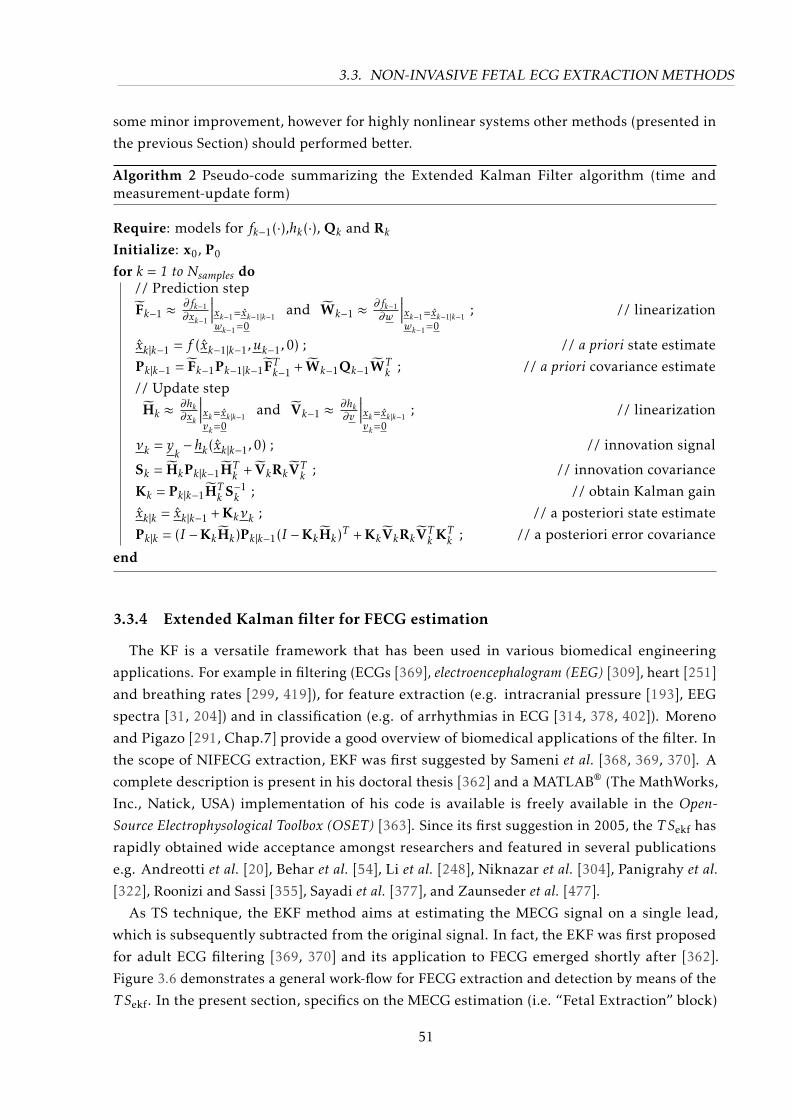
3.3. NON-INVASIVE FETAL ECG EXTRACTION METHODS
some minor improvement, however for highly nonlinear systems other methods (presented in
the previous Section) should performed better.
Algorithm 2 Pseudo-code summarizing the Extended Kalman Filter algorithm (time andmeasurement-update form)
Require: models for fk−1(·),hk(·), Qk and RkInitialize: x0, P0
for k = 1 to Nsamples do// Prediction step
Fk−1 ≈ ∂fk−1∂xk−1
∣∣∣∣wk−1=0xk−1=xk−1|k−1
and Wk−1 ≈ ∂fk−1∂w
∣∣∣∣wk−1=0xk−1=xk−1|k−1
; // linearization
xk|k−1 = f (xk−1|k−1,uk−1,0) ; // a priori state estimate
Pk|k−1 = Fk−1Pk−1|k−1FTk−1 + Wk−1Qk−1WTk ; // a priori covariance estimate
// Update step
Hk ≈ ∂hk∂xk
∣∣∣∣vk=0xk=xk|k−1
and Vk−1 ≈ ∂hk∂v
∣∣∣∣vk=0xk=xk|k−1
; // linearization
νk = yk− hk(xk|k−1,0) ; // innovation signal
Sk = HkPk|k−1HTk + VkRkVT
k ; // innovation covariance
Kk = Pk|k−1HTk S−1
k ; // obtain Kalman gain
xk|k = xk|k−1 + Kkνk ; // a posteriori state estimate
Pk|k = (I −KkHk)Pk|k−1(I −KkHk)T + KkVkRkVTk KT
k ; // a posteriori error covariance
end
3.3.4 Extended Kalman filter for FECG estimation
The KF is a versatile framework that has been used in various biomedical engineering
applications. For example in filtering (ECGs [369], electroencephalogram (EEG) [309], heart [251]
and breathing rates [299, 419]), for feature extraction (e.g. intracranial pressure [193], EEG
spectra [31, 204]) and in classification (e.g. of arrhythmias in ECG [314, 378, 402]). Moreno
and Pigazo [291, Chap.7] provide a good overview of biomedical applications of the filter. In
the scope of NIFECG extraction, EKF was first suggested by Sameni et al. [368, 369, 370]. A
complete description is present in his doctoral thesis [362] and a MATLAB® (The MathWorks,
Inc., Natick, USA) implementation of his code is available is freely available in the Open-Source Electrophysological Toolbox (OSET) [363]. Since its first suggestion in 2005, the T Sekf has
rapidly obtained wide acceptance amongst researchers and featured in several publications
e.g. Andreotti et al. [20], Behar et al. [54], Li et al. [248], Niknazar et al. [304], Panigrahy et al.[322], Roonizi and Sassi [355], Sayadi et al. [377], and Zaunseder et al. [477].
As TS technique, the EKF method aims at estimating the MECG signal on a single lead,
which is subsequently subtracted from the original signal. In fact, the EKF was first proposed
for adult ECG filtering [369, 370] and its application to FECG emerged shortly after [362].
Figure 3.6 demonstrates a general work-flow for FECG extraction and detection by means of the
T Sekf. In the present section, specifics on the MECG estimation (i.e. “Fetal Extraction” block)
51
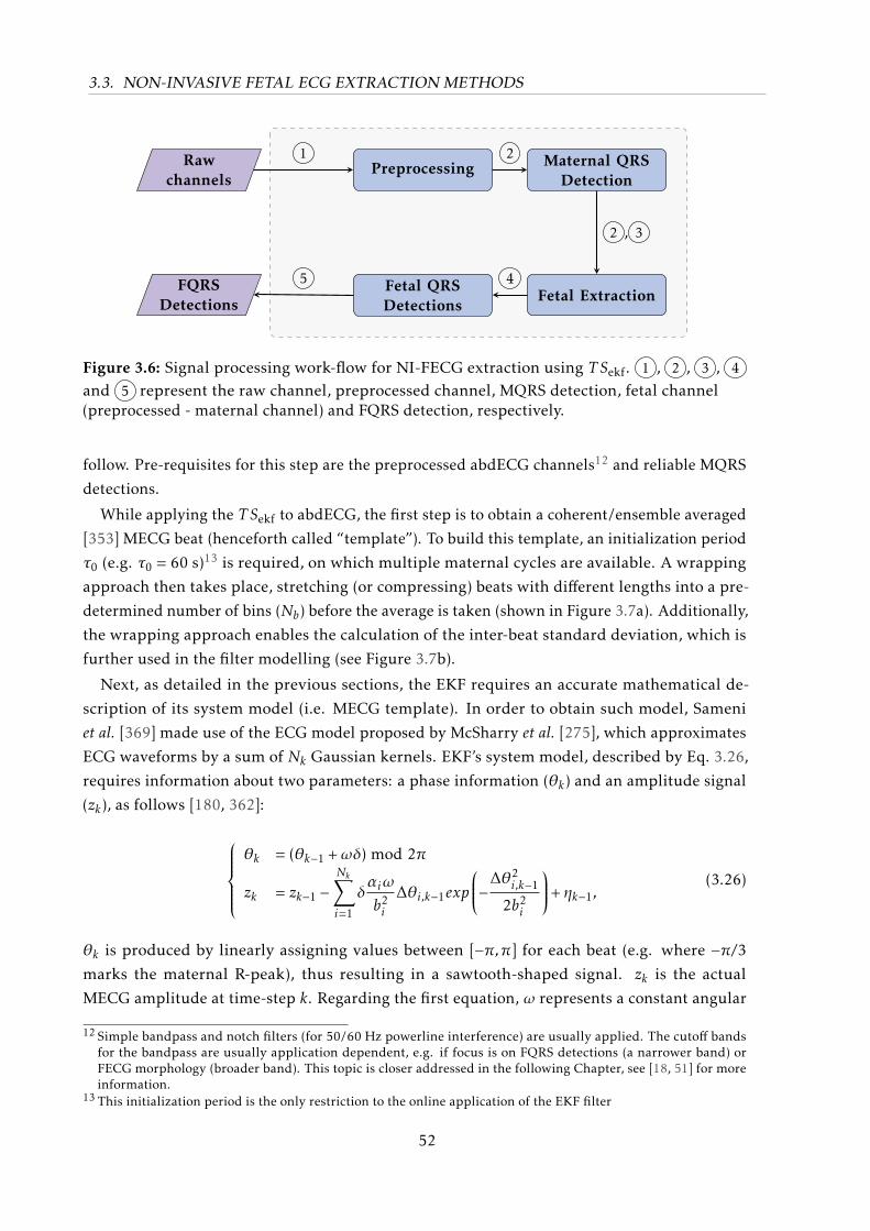
3.3. NON-INVASIVE FETAL ECG EXTRACTION METHODS
Rawchannels
Preprocessing Maternal QRSDetection
Fetal ExtractionFetal QRSDetections
FQRSDetections
1 2
2 , 3
45
Figure 3.6: Signal processing work-flow for NI-FECG extraction using T Sekf. 1 , 2 , 3 , 4
and 5 represent the raw channel, preprocessed channel, MQRS detection, fetal channel(preprocessed - maternal channel) and FQRS detection, respectively.
follow. Pre-requisites for this step are the preprocessed abdECG channels12 and reliable MQRS
detections.
While applying the T Sekf to abdECG, the first step is to obtain a coherent/ensemble averaged
[353] MECG beat (henceforth called “template”). To build this template, an initialization period
τ0 (e.g. τ0 = 60 s)13 is required, on which multiple maternal cycles are available. A wrapping
approach then takes place, stretching (or compressing) beats with different lengths into a pre-
determined number of bins (Nb) before the average is taken (shown in Figure 3.7a). Additionally,
the wrapping approach enables the calculation of the inter-beat standard deviation, which is
further used in the filter modelling (see Figure 3.7b).
Next, as detailed in the previous sections, the EKF requires an accurate mathematical de-
scription of its system model (i.e. MECG template). In order to obtain such model, Sameni
et al. [369] made use of the ECG model proposed by McSharry et al. [275], which approximates
ECG waveforms by a sum of Nk Gaussian kernels. EKF’s system model, described by Eq. 3.26,
requires information about two parameters: a phase information (θk) and an amplitude signal
(zk), as follows [180, 362]:
θk = (θk−1 +ωδ) mod 2π
zk = zk−1 −Nk∑i=1
δαiω
b2i
∆θi,k−1exp
−∆θ2i,k−1
2b2i
+ ηk−1,(3.26)
θk is produced by linearly assigning values between [−π,π] for each beat (e.g. where −π/3marks the maternal R-peak), thus resulting in a sawtooth-shaped signal. zk is the actual
MECG amplitude at time-step k. Regarding the first equation, ω represents a constant angular
12 Simple bandpass and notch filters (for 50/60 Hz powerline interference) are usually applied. The cutoff bandsfor the bandpass are usually application dependent, e.g. if focus is on FQRS detections (a narrower band) orFECG morphology (broader band). This topic is closer addressed in the following Chapter, see [18, 51] for moreinformation.
13 This initialization period is the only restriction to the online application of the EKF filter
52
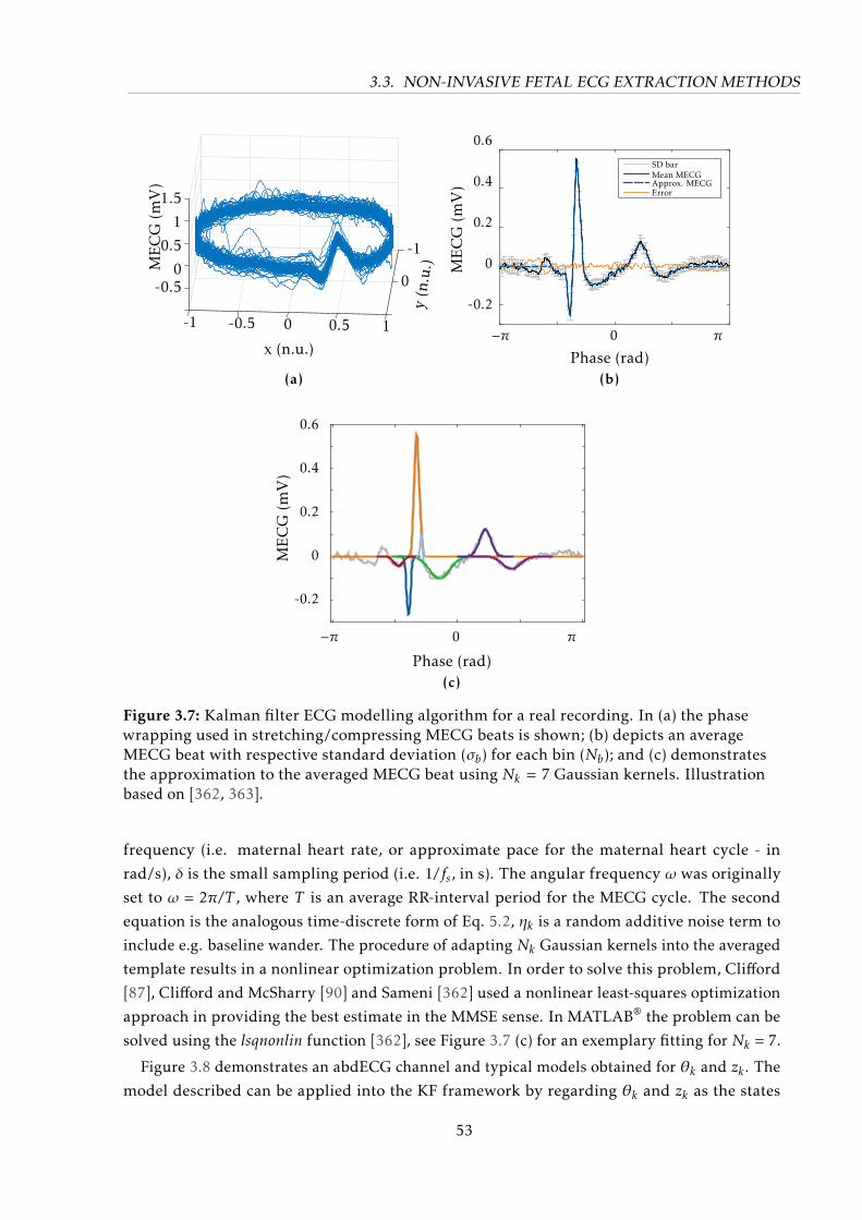
3.3. NON-INVASIVE FETAL ECG EXTRACTION METHODS
y(n
.u.)
-1
0
10.5
x (n.u.)
0-0.5-1
1.5
1
0.5
0-0.5
ME
CG
(mV
)
(a)Phase (rad)
0.6
0.4
0.2
0
-0.2
−π 0 π
ME
CG
(mV
)
SD barMean MECGApprox. MECGError
(b)
Phase (rad)
0.6
0.4
0.2
0
-0.2
−π 0 π
ME
CG
(mV
)
(c)
Figure 3.7: Kalman filter ECG modelling algorithm for a real recording. In (a) the phasewrapping used in stretching/compressing MECG beats is shown; (b) depicts an averageMECG beat with respective standard deviation (σb) for each bin (Nb); and (c) demonstratesthe approximation to the averaged MECG beat using Nk = 7 Gaussian kernels. Illustrationbased on [362, 363].
frequency (i.e. maternal heart rate, or approximate pace for the maternal heart cycle - in
rad/s), δ is the small sampling period (i.e. 1/fs, in s). The angular frequency ω was originally
set to ω = 2π/T , where T is an average RR-interval period for the MECG cycle. The second
equation is the analogous time-discrete form of Eq. 5.2, ηk is a random additive noise term to
include e.g. baseline wander. The procedure of adapting Nk Gaussian kernels into the averaged
template results in a nonlinear optimization problem. In order to solve this problem, Clifford
[87], Clifford and McSharry [90] and Sameni [362] used a nonlinear least-squares optimization
approach in providing the best estimate in the MMSE sense. In MATLAB® the problem can be
solved using the lsqnonlin function [362], see Figure 3.7 (c) for an exemplary fitting for Nk = 7.
Figure 3.8 demonstrates an abdECG channel and typical models obtained for θk and zk . The
model described can be applied into the KF framework by regarding θk and zk as the states
53
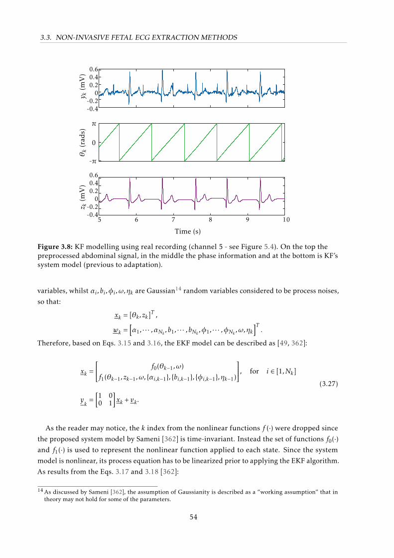
3.3. NON-INVASIVE FETAL ECG EXTRACTION METHODS
y k(m
V)
0.60.40.2
0-0.2-0.4
θk
(rad
s)
-π
0
π
5 6 7 8 9 10
z k(m
V)
0.60.40.2
0-0.2-0.4
Time (s)
Figure 3.8: KF modelling using real recording (channel 5 - see Figure 5.4). On the top thepreprocessed abdominal signal, in the middle the phase information and at the bottom is KF’ssystem model (previous to adaptation).
variables, whilst αi ,bi ,φi ,ω,ηk are Gaussian14 random variables considered to be process noises,
so that:
xk = [θk , zk]T ,
wk =[α1, · · · ,αNk ,b1, · · · ,bNk ,φ1, · · · ,φNk ,ω,ηk
]T.
Therefore, based on Eqs. 3.15 and 3.16, the EKF model can be described as [49, 362]:
xk =
f0(θk−1,ω)
f1(θk−1, zk−1,ω, αi,k−1, bi,k−1, φi,k−1,ηk−1)
, for i ∈ [1,Nk]
yk
=[1 00 1
]xk + vk .
(3.27)
As the reader may notice, the k index from the nonlinear functions f (·) were dropped since
the proposed system model by Sameni [362] is time-invariant. Instead the set of functions f0(·)and f1(·) is used to represent the nonlinear function applied to each state. Since the system
model is nonlinear, its process equation has to be linearized prior to applying the EKF algorithm.
As results from the Eqs. 3.17 and 3.18 [362]:
14 As discussed by Sameni [362], the assumption of Gaussianity is described as a “working assumption” that intheory may not hold for some of the parameters.
54

3.3. NON-INVASIVE FETAL ECG EXTRACTION METHODS
Fk−1 ≈ ∂f
∂xk−1
∣∣∣∣∣∣wk−1=0xk−1=xk−1|k−1
∂f0∂θk−1
=∂f1∂zk−1
= 1,∂f0∂zk−1
= 0
∂f1∂θk−1
= −Nk∑i=1
δαiω
b2i
1− ∆θ2i,k−1
b2i
exp−∆θ2i,k−1
2b2i
,Wk−1 ≈ ∂f
∂w
∣∣∣∣∣wk−1=0xk−1=xk−1|k−1
(3.28)
∂f0∂αi
=∂f0∂bi
=∂f0∂φi
=∂f0∂ηk−1
= 0,∂f1∂ηk−1
= 1,∂f0∂ω
= δ
∂f1∂αi
= −δω∆θi,k−1
b2i
exp
−∆θ2i,k−1
2b2i
,∂f1∂bi
= 2δαiω∆θi,k−1
b3i
1− ∆θ2i,k−1
2b2i
exp−∆θ2i,k−1
2b2i
,∂f1∂φi
= δαiω
b2i
1− ∆θ2i,k−1
b2i
exp−∆θ2i,k−1
2b2i
,∂f1∂ω
= −∑i=1
δαi∆θ
2i,k−1
b2i
exp
−∆θ2i,k−1
2b2i
∀i ∈ [1,Nk].
So far, the nonlinear system model and its linearization procedure for applying the EKF
on abdominal signals were described. As explained in Section 3.3.2, the initialization of the
algorithm’s covariance matrices plays an important role in the performance of the EKF. Based on
[49, 362, 363] the following initial parameters for the state and the filter’s covariance matrices
can be defined:
Qk = Q0 = diag([σ2α1..αNk , σ
2b1..bNk
, σ2φ1..φNk
, σ2ω , σ
2f it
])Rk = R0 =
(ωδ)2 0
0 σ2f it
P0 =
(2π)2 0
0 10 ∗max(|y1:τ0|2)
(3.29)
where diag(·) is a function which diagonalizes its argument, σ2x with x = αi ,bi ,φi ,ω represents
the manually defined variance for each Gaussian parameter and angular frequency, σ2f it =
1/Nb∑b σ
2f it(b) is the mean standard deviation obtained during the template fitting for all bins
(see Figure 3.7-(b)) andmax(·) returns the maximum value of its argument. On its simplest form,
Sameni [362] definedQk and Rk as time-invariant, thusQ0 and R0. As explained in Section 3.3.2,
KF’s performance depends on its model and the tunning of its covariance matrices. Therefore,
the parameters described in Equation 3.29 should be exhaustively calibrated depending on
the application (e.g. electrode configuration). Considering that this tunning is satisfactory,
55
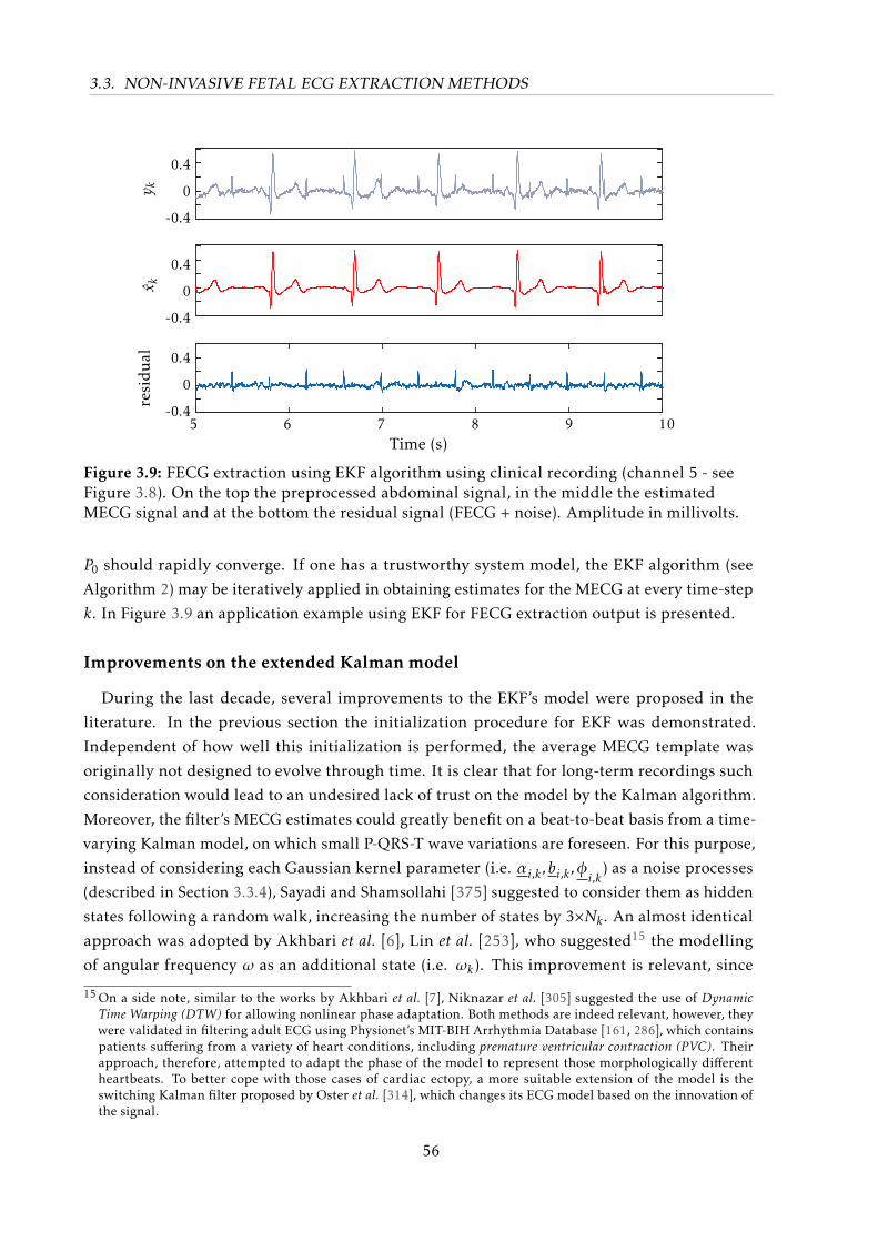
3.3. NON-INVASIVE FETAL ECG EXTRACTION METHODS
y kx k
resi
dual
0.4
0
-0.4
0.4
0
-0.4
0.4
0
-0.45 6 7 8 9 10
Time (s)
Figure 3.9: FECG extraction using EKF algorithm using clinical recording (channel 5 - seeFigure 3.8). On the top the preprocessed abdominal signal, in the middle the estimatedMECG signal and at the bottom the residual signal (FECG + noise). Amplitude in millivolts.
P0 should rapidly converge. If one has a trustworthy system model, the EKF algorithm (see
Algorithm 2) may be iteratively applied in obtaining estimates for the MECG at every time-step
k. In Figure 3.9 an application example using EKF for FECG extraction output is presented.
Improvements on the extended Kalman model
During the last decade, several improvements to the EKF’s model were proposed in the
literature. In the previous section the initialization procedure for EKF was demonstrated.
Independent of how well this initialization is performed, the average MECG template was
originally not designed to evolve through time. It is clear that for long-term recordings such
consideration would lead to an undesired lack of trust on the model by the Kalman algorithm.
Moreover, the filter’s MECG estimates could greatly benefit on a beat-to-beat basis from a time-
varying Kalman model, on which small P-QRS-T wave variations are foreseen. For this purpose,
instead of considering each Gaussian kernel parameter (i.e. αi,k ,bi,k ,φi,k) as a noise processes
(described in Section 3.3.4), Sayadi and Shamsollahi [375] suggested to consider them as hidden
states following a random walk, increasing the number of states by 3×Nk . An almost identical
approach was adopted by Akhbari et al. [6], Lin et al. [253], who suggested15 the modelling
of angular frequency ω as an additional state (i.e. ωk). This improvement is relevant, since
15 On a side note, similar to the works by Akhbari et al. [7], Niknazar et al. [305] suggested the use of DynamicTime Warping (DTW) for allowing nonlinear phase adaptation. Both methods are indeed relevant, however, theywere validated in filtering adult ECG using Physionet’s MIT-BIH Arrhythmia Database [161, 286], which containspatients suffering from a variety of heart conditions, including premature ventricular contraction (PVC). Theirapproach, therefore, attempted to adapt the phase of the model to represent those morphologically differentheartbeats. To better cope with those cases of cardiac ectopy, a more suitable extension of the model is theswitching Kalman filter proposed by Oster et al. [314], which changes its ECG model based on the innovation ofthe signal.
56

3.3. NON-INVASIVE FETAL ECG EXTRACTION METHODS
on the original filter equation (see Eq. 3.26) no additive noise was associated with the phase
information. Lastly, as proposed by [305], a random additive noise (ηθ,k) was added to the
phase state equation so that the phase is no longer “strictly” linear, but fluctuations around
its modelled values are allowed. Therefore, the resulting model with 3×Nk + 1 [6, 305, 375]
additional state variables is summarized as follows:
f0 : θk+1 = (θk +ωkδ) mod 2π+ ηθ,k
f1 : zk+1 = zk−1 −Nk∑i=1δαiw
b2i
∆θi,k−1exp(−∆θ2i,k−1
2b2i
) + ηz,k−1
f2 : ωk =ωk−1 + ε1,k−1
f3 : α1,k = α1,k−1 + ε2,k−1...
fNk+2 : αNk ,k = αNk ,k−1 + ε(Nk+1),k−1
fNk+3 : b1,k = b1,k−1 + ε(Nk+2),k−1...
f2·Nk+2 : bNk ,k = bNk ,k−1 + ε(2·Nk+1),k−1
f2·Nk+3 : φ1,k = φ1,k−1 + ε(2·Nk+2),k−1...
f3·Nk+2 : φNk ,k = φNk ,k−1 + ε(3·Nk+1),k−1
(3.30)
so that the state xk and noise process wk become:
xk =[θk , zk ,ωk , α1:Nk ,k, b1:Nk ,k, φ1:Nk ,k
]Twk =
[ηθ,k ,ηz,kε1:3·Nk+1,k
]T . (3.31)
The new state equations may be linearized as in Eq. 3.28 [49, 180, 375]:
Fk−1 ≈ ∂f
∂xk−1
∣∣∣∣∣∣wk−1=0xk−1=xk−1|k−1
∂f0∂θk−1
=∂f1∂zk−1
= 1,∂f0∂ωk−1
= δ,
∂f0∂zk−1
=∂f0
∂αi,k−1=
∂f0∂bi,k−1
=∂f0
∂φi,k−1= 0,
∂f1∂θk−1
= −∑i
δαi,k−1ω
b2i,k−1
1− ∆θ2i,k−1
b2i,k−1
exp−∆θ2i,k−1
2b2i,k−1
, (3.32)
∂f1∂ωk−1
= −∑i=1
δαi∆θ
2i,k−1
b2i
exp
−∆θ2i,k−1
2b2i
,∂f1
∂αi,k−1= −δω∆θi,k−1
b2i,k−1
exp
−∆θ2i,k−1
2b2i,k−1
,57

3.3. NON-INVASIVE FETAL ECG EXTRACTION METHODS
∂f1∂bi,k−1
= 2δαiω∆θi,k−1
b3i,k−1
1− ∆θ2i,k−1
2b2i,k−1
exp−∆θ2i,k−1
2b2i,k−1
, (3.32 cont.)
∂f1∂φi,k−1
= δαiω
b2i,k−1
1− ∆θ2i,k−1
b2i,k−1
exp−∆θ2i,k−1
2b2i,k−1
,
∂fi
∂xj+1k−1
being x
jk−1is the jth variable in state vector x
1, if ∀i = j |i = 2,3, · · · ,3·Nk + 20, otherwise
Wk−1 =∂f
∂w
∣∣∣∣∣wk−1=0xk−1=xk−1|k−1
≈ I(3·Nk+3)×(3·Nk+3) (3.33)
Another improvement proposed by Sameni et al. [370], Tarvainen et al. [420] was adapting
the covariance matrix Rk by using a normalized innovation for state zk such that:
ci =1N
i∑k=i−N+1
(νk)2
sk(3.34)
where νk is the second entry of the innovation vector νk presented in Eq. 3.8 that refers to
the MECG amplitude state zk. Similarly, sk is the second diagonal entry of filter-calculated
innovation matrix Sk (see Eq. 3.9). The factor ci then normalizes the estimated innovation for zkover its estimated variance sk using a moving average window of length N . Such approach, also
present in [166, Sec. 8.11], is termed as information-weighted square innovation. According to
[370], ideally is ci ≈ 1, if it has values greater than unit the innovation signal variance is being
underestimated, while values close to zeros indicate it is being overestimated. The authors then
adaptively updated the matrix Rk by using a AR moving average window of length M:
s2k = λvs2k−1 + (1−λv)
1M
k−1∑j=k−M
(sj)2
(3.35)
where 0 < λv < 1 is a forgetting factor, set to λv = 0.95 in [420]. If M > 1, the adaptation repre-
sents a moving average filter with the ω changing the slope of the filter’s response, otherwise
it is a first order AR model as in [420]. For updating the second entry q2k of the model noise
covariance Qk , Tarvainen et al. [420] proposes the following correction factor:
q2k = λw
s2kp2k
(3.36)
where p2k is the second diagonal entry of matrix Pk|k and λw is the update coefficient, empirically
defined. The observation variance (s2k ) is included in order to remove the influence of signal
amplitude of the estimate.
58
3.4. FETAL QRS DETECTION
Further extensions
In Section 3.3.3 several extensions of the linear Kalman filter were presented. Aside from
the EKF, the UKF [370] and Particle Filters [253] have also been applied in the scope of adult
ECG denoising, which could be simply applied to NIFECG signals. In [365], the use of Particle
filters is suggested as future work, however, to date there are no studies known to the author
who applied McSharry’s ECG model using such filters.
Additionally, if a delay in our filter or offline processing is allowed, smoothing may be used.
There are 3 types of smoothing filters: fixed-point, fixed-lag and fixed-interval. In fixed-point
smoothing, the point one intends to estimate is fixed, but the number of measurements continu-
ally changes. Fixed-lag smoothers allow a constant lag of some samples between the newest
measurement and the current estimated sample. The last, and in our case most relevant, type
is fixed-interval smoothing. Fixed-interval smoothers process in batches a fixed interval of
measurements, using all available samples [399, Chap.9], i.e. offline processing. The ExtendedKalman Smoother (EKS) is another extension of the EKF which enables the use of future infor-
mation into improving the current estimate. The EKS algorithm consists of a forward EKF stage
followed by a backward recursive smoothing stage. Due to its non-causal nature, the EKS is
expected outperform the EKF [377].
In [370] a comparison between the EKF, EKS and UKF is presented. According to the authors,
EKS demonstrated the smoothest results, while UKF performed better than EKF. Moreover,
the authors affirmed that the most remarkable differences in estimation occur around sharp
turning points of the signal (e.g. QRS complexes), where derivative-free methods such as UKF
are better suited for strong non-linearities [370]. Based on the presented state-of-the-art on the
EKF model, novel improvements are proposed further in Chapter 4.
3.4 Fetal QRS Detection
Analogous to the analysis of adult electrocardiography, the FQRS complexes obtained from
FECG signals provide a first interesting feature, which can be directly linked to clinical diagnos-
tic information. The current state-of-the-art for FQRS detectors are discussed in this section,
meanwhile multi-channel merging considerations are presented in Section 3.4.1 and statistical
metrics for evaluating these detector’s accuracy and precision are described in Section 3.4.2.
From FQRS detections, one can almost directly derive the FHR (described in Section 3.5) and ob-
tain FHRV parameters (Section 2.3.1). However, the importance of accurate FQRS is not limited
to FHR and FHRV analysis. In fact, reliable detection of fetal peak locations is pre-requirement
for further analysis of FECG’s morphology, since FQRS locations are crucial for segmentation of
the FECG cycle.
Several algorithms have been proposed in the literature for QRS detection in adult ECG.
A comprehensive overview on those methods can be found in Köhler et al. [232]. For the
sake of example, methods may be based on adaptive thresholding [171, 320], filter-banks [3],
matched-filters [123, 220], slope-detection [5, 416] or in representations such as the Hilbert [58]
59
3.4. FETAL QRS DETECTION
or Wavelet transforms [154, 247].
Fetal QRS detectors present in the literature are usually adaptations of adult QRS detectors to
cope with the higher FHR. During the PCINC 2013 several participants made use of this strategy,
including some open-source entries available at Physionet e.g. Behar et al. [54] proposed an
adapted implementation of the Pan and Tompkins [320] algorithm. Another relevant source
of FQRS detection methods is the OSET [363], which includes a maxima search algorithm.
Other examples of this strategy are matched filters [169, 254], slope-detection [337], supervised
machine learning using the ESN algorithm [255], Wavelet transform [9, 155, 269]. Aside from
the PCINC 2013, there is to date no study evaluating the performance of those FQRS detectors
against each other known to the author. Some authors separate the FQRS procedure performed
after FECG extraction (see Figure 3.6) into a “FECG enhancement” and “FQRS detection” step.
In this work, however, the preprocessing performed to enhance the fetal peaks (i.e. feature
extraction) is regarded as part of the FQRS algorithm.
3.4.1 Merging multichannel fetal QRS detections
Most FQRS detectors available in the literature make use of a single extracted FECG channel.
However, real applications usually make use of multi-lead systems (as discussed in Section 3.2.3).
In order to cope profit from this higher data dimensionality, one can either select/merge the
available FECG channels (i.e. prior to FQRS detection), or select/merge the different FQRS
detections available. In any case, some sort of metric for fetal signal quality (i.e. signal qualityindex (SQI)) has to be applied for determining which lead(s) to use. Typical measures take
in consideration: 1) the morphology of the FECG signal, such as a kurtosis as “peakedness”
measure; or 2) the pseudo-peridicity of the FQRS detections, i.e. a RR interval regularity.
Therefore, performing the selection/merge after the FQRS detection occurs is advantageous
since a regularity metric for each FECG channel is then available.
While the selection of one single FQRS source to represent the whole measurement may
work in short datasets (e.g. PCINC 201316) , it is sub-optimal for long-term recordings due to
the varying nature of the fetal signal’s SNR. Therefore, adaptively fusion of the information
contained in multiple FQRS detections is a more attractive solution. One solution is to adaptively
(e.g. on every few seconds) choose the lead with the best SQI, the so-called lead switchingapproach. An exemplary application of such method was proposed by Johnson et al. [209, 211],
who made use of several SQI measures and lead switching to multi-modal adult beat detection
in obtaining the best scores on the PCINC 2014. Another option is to use weighted or majority
voting to obtain a consensus detections. Such approaches have been often for merging the results
of different QRS detectors/classifiers [205, 283] and for producing consensus from annotations
provided by different experts [170, 429, 479].
16 Behar et al. [54] obtain top-scoring results in the PCINC 2013 by making use of a regularity SQI in selecting themost periodic FQRS detection source. The method proposed by the author not only used every lead, but alsoextracted channels using different extraction methods.
60
3.4. FETAL QRS DETECTION
3.4.2 Detection performance
In order to report FQRS detection statistics different measures were proposed in the literature.
The main goal of these metrics is to assess the accuracy and precision of the obtained FQRS
detections. In an attempt to standardize this assessment, challenge organisers at PCINC 2013
suggested the use of the root mean square error (RMSE) of corresponding RR intervals as scoring
measure for its events 2 and 5 (E2/E5 - in ms) [20, 395]:
E2/E5 =
√√√√1Np
N ′p∑n=1
(RRtn −RRrn
)2(in ms) (3.37)
being n the detection index, Np the number of existent reference FQRS anotations, N ′p the
number of FQRS detections available, RRtn each detected RR interval (t = test) and RRrn the
nearest reference (r) RR interval available. However, the measure mixes both precision and
accuracy in one score, which is not optimal for the interpretation of the results.
In order to more clearly present the accuracy of FQRS detections, measures presented in the
American National Standards Institute (ANSI) [26] can be used. Particularly, the number of truepositive (TP) denotes correctly detected peaks, false negative (FN) being existing peaks which
were not detected and false positive (FP) nonexistent peaks that were falsely detected can be
reported. Differing from the adult norm [26] of 150 ms acceptance interval between detection
and reference annotation, to account for the higher FHR a window of 50 ms is usually applied
[20, 52, 477]. Based on from these absolute numbers, the following summary metrics can be
used:
SE = 100 · T PT P +FN
(in %) P P V = 100 · T PT P +FP
(in %) (3.38)
where sensitivity (SE) measures the percentage of actual FQRS complexes that were correctly
identified and positive predictive value (PPV) defines the proportion of detected peaks that
indeed correspond to FQRS peaks. Once again, these measures can be condesed into two FQRS
detection accuracy measures, namely accuracy (ACC) [221] and the F1 score [52, 374]:
ACC = 100 · T PT P +FN +FP
[%] (3.39)
F1 = 100 · 2 · P P V · SEP P V + SE
= 100 · 2 · T P2 · T P +FN +FP
(in %) (3.40)
ACC is simply the percentage of the correctly detected peaks, over all detected and un-detected
peaks, while F1 provides the harmonic mean between SE and P P V , therefore summarizing
those measures in one score. Despite some criticism [339, 340], the latter measure is particularly
suitable for situations when the average of rates is desired [51, 374].
Beyond the presented metrics for evaluating FQRS’s window-based accuracy (i.e. SE, P P V
and F1), a distance measure is necessary to discriminate between precise and imprecise detec-
tions, e.g. if any jitter occurs, information which is not captured by window-based metrics.
Andreotti et al. [18] suggest the used of the mean average error (MAE). MAE consists of the
absolute time difference between the reference annotation time-stamp (QRSrn) and detected
61
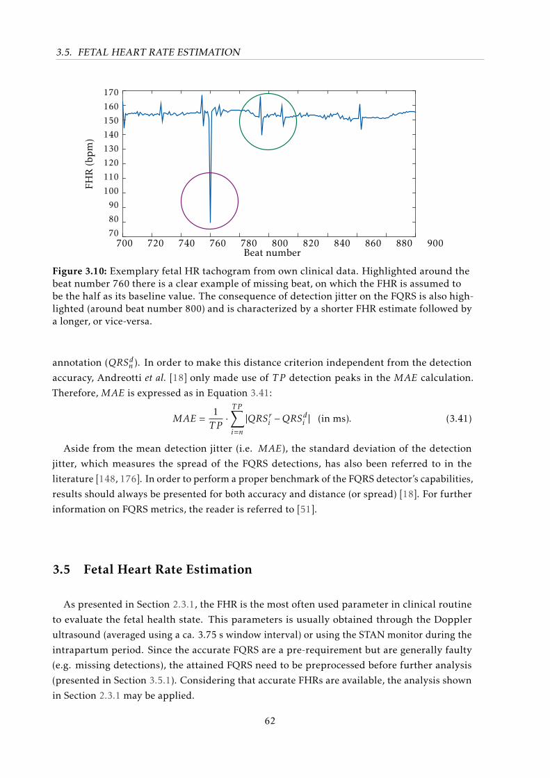
3.5. FETAL HEART RATE ESTIMATION
Beat number700 720 740 760 780 800 820 840 860 880 900
FHR
(bp
m)
170
160
150
140
130
120
110
100
90
80
70
Figure 3.10: Exemplary fetal HR tachogram from own clinical data. Highlighted around thebeat number 760 there is a clear example of missing beat, on which the FHR is assumed tobe the half as its baseline value. The consequence of detection jitter on the FQRS is also high-lighted (around beat number 800) and is characterized by a shorter FHR estimate followed bya longer, or vice-versa.
annotation (QRSdn ). In order to make this distance criterion independent from the detection
accuracy, Andreotti et al. [18] only made use of T P detection peaks in the MAE calculation.
Therefore, MAE is expressed as in Equation 3.41:
MAE =1T P·T P∑i=n
|QRSri −QRSdi | (in ms). (3.41)
Aside from the mean detection jitter (i.e. MAE), the standard deviation of the detection
jitter, which measures the spread of the FQRS detections, has also been referred to in the
literature [148, 176]. In order to perform a proper benchmark of the FQRS detector’s capabilities,
results should always be presented for both accuracy and distance (or spread) [18]. For further
information on FQRS metrics, the reader is referred to [51].
3.5 Fetal Heart Rate Estimation
As presented in Section 2.3.1, the FHR is the most often used parameter in clinical routine
to evaluate the fetal health state. This parameters is usually obtained through the Doppler
ultrasound (averaged using a ca. 3.75 s window interval) or using the STAN monitor during the
intrapartum period. Since the accurate FQRS are a pre-requirement but are generally faulty
(e.g. missing detections), the attained FQRS need to be preprocessed before further analysis
(presented in Section 3.5.1). Considering that accurate FHRs are available, the analysis shown
in Section 2.3.1 may be applied.
62
3.5. FETAL HEART RATE ESTIMATION
3.5.1 Preprocessing the fetal heart rate
Despite one’s best effort on obtaining accurate detections, FQRS are usually imperfectly
identified. These inaccuracies may have physiological, pathological or technical origins [326].
For instance, according to Clifford et al. [88], the fiducial markers should always be set on the
onset of the P-wave rather than on the R-peaks, since this is a more accurate marker of the
sinoatrial node stimuli. However, the R-peaks are considerably simpler to detect, particularly in
the NIFECG case. Aside from this technical difficulty, several other aspects should be considered.
Peltola [326] presents an overview on available methods for preprocessing HR tachograms, while
Clifford [86] provide a more in-depth analysis of available methods.
The RR series obtained from ECG recordings are usually functions of the number of heartbeats
instead of time (usually in beats per minute (bpm)) [249]. Figure 3.10 exhibits an exemplary fetal
RR series tachogram, obtained by taking the first derivative of the FQRS timestamps (in s) and
dividing its inverse. As Figure 3.10 hints, some of the common difficulties encountered when
analyzing FHRV. These may have a technical (e.g. detection jitter, missing detections or uneven
sampling) or a pathophysiological origin (e.g. ectopic beats). Different preprocessing methods
are available in the literature to treat each of these events. Despite being an interesting research
topic, such techniques to process heart rate series exceed the scope of this work. As previously
explained, this work focuses on more fundamental problems in the signal processing of FHR
rather than clinically interpreting those results. For this reason, in this work 5 seconds moving
median windows with 1 second overlap were applied when calculating FHR estimates. This
approach is specifically applied in Section 4.3.2, where a multichannel approach to improve
FHR estimates is proposed.
3.5.2 Fetal heart rate statistics
Similarly to the F1 accuracy metric presented for FQRS detections, the heart rate detectionrate (HDR) has been often applied in adult HR detection. HDR assesses the percentage of the HR
values within ±5 bpm tolerance [27] of the reference HR annotations (regarded as TP estimates)
[51, 52]. On the fetal case, this tolerance was modified to ±10 bpm to reflect the higher FHR
(accelerations and decelerations of the FHR are usually defined by changes greater than 15 bpm
[12]). HDR results (in percent) are given by dividing the number of TP by the total number of
measured FHR estimates [22], i.e. similar to Eq. 3.39, as follows:
HDR = 100 · T PT P +FN +FP
(in %) (3.42)
As for precision metric, the distance between the produced FHR and the reference values were
also often used in the literature. Its use is particularly relevant when some averaging window
is applied in producing the RR estimates (e.g. CTG’s 3.75 s averaged FHR values). During the
PCINC 2013, the mean square error between matched reference and test FHR measurements
(i.e. FHRr and FHRt, respectively) at 12 instances for each recording (on every 5 s) [20, 51, 395].
63
3.6. FETAL ECG MORPHOLOGICAL ANALYSIS
The scoring statistic was used for the Events 1 and 4 (E1/4 - in bpm2):
E1/E4 =1
12
12∑i=1
(FHRtn −FHRrn
)2(in bpm2) (3.43)
As before, the Challenge scoring is hardly interpretable and depends on pre-defined Physionet
WFDB functions (see [161, 398]). In this work, a more straightforward measure is used, namely
the RMSE between reference and test FHR, described as:
RMSE =
√√√√1Np
N ′p∑n=1
(FHRtn −FHRrn
)2(in bpm) (3.44)
3.6 Fetal ECG Morphological Analysis
In Section 2.3.2 the three major parameters used in fetal morphological analysis were clarified,
namely the FQT, FST and the FTQRS. Due to the lack of standards for FECG morphological
analysis, there are several aspects of this evaluation that require further investigation. In
this section, focus is put on the signal processing tools that enable the derivation of these
morphological features. Further on, metrics on how to evaluate the accuracy of such estimated
measures are proposed.
The first aspect to be regarded is the bandwidth used while extracting the NIFECG signal,
since it can deform the fetal signal, e.g. the T-wave. Throughout this work the signal bandwidth
was configured as recommended by the American Heart Society for adult electrocardiography
[231] (as further described in Section 4.1). Similarly, the extraction method used (see Sec-
tion 3.3.1) is expected to have an impact on those parameter estimates and are evaluated in
Chapter 6.
Another important consideration is whether the morphological features should be obtained
on a beat-to-beat basis or on an averaged FECG template. The first option is obviously more
attractive, however due to the usually low SNR of the fetal signal it is impracticable, making the
use of averaged FECG beats imperative17. As an example, even though direct FSE recordings
comprise a much higher FECG SNR, commercial equipments such as STAN, still makes use
of this averaging procedure. For this reason, this work is restricted to the analysis of FECG
template beats. A general signal processing scheme for obtaining the aforementioned features is
presented in Figure 3.11.
Template generation plays an important role in this analysis, important details are the
number of average beats, which central tendency measure is used (e.g. mean, median), and if
low correlating or ectopic beats are excluded from final template. In preliminary works [18] the
template construction method proposed by Oster et al. [314] has provided better results than
similar methods, therefore it is used in this thesis.
The template generation step is followed by beat segmentation, which aims at finding the
17 On a side note, in fact, even for adult ECG analysis there are no current standards and signal-averaging is not aconsensus among researchers, despite its wide usage in the literature (e.g. [85, 132, 162, 473])
64

3.7. PROBLEM DESCRIPTION
Extracted +unmixed FECGFQRS reference
Templatesgeneration
ECGSegmentation
Heuristictreatment
Results forFQT and
˜FTQRS
Figure 3.11: Signal processing steps for morphological analysis, regarding morphological featuresshown in Figure 2.2.
necessary fiducial points, i.e. locations for Q-onset, T-offset as well as T-peak. Several ECG
segmentation algorithms have been proposed in the literature [203, 269, 376, 381, 451], however
current algorithms are mainly designed and trained using adult ECG databases and are likely to
be sub-optimal for FECG analysis. To the authors best knowledge, the only FECG segmentation
algorithm present in the literature is an adaptation by Hurezeanu et al. [195] of the Wavelet
delineation algorithm from Martinez et al. [269]. Additionally, despite the large number of adult
segmentation algorithms available, only a very few of those have been made open-source such
as: the ecgpuwave [203], as part of the WFDB toolbox [161, 398]18, and very recently the Wavelet
delineation script [269], made available under the ecg-kit19. As demonstrated in Figure 3.11,
the last step is an heuristic treatment of the obtained fiducial locations. This simple step is
necessary for making sure that the fiducial annotations are valid, e.g. from the physiology not
too short/long.
At last, one can define the FQT and FTQRS errors as [18]:
FQT =1N
N∑i=1
∣∣∣FQTabdm −FQTref ∣∣∣ (in ms) (3.45)
˜FTQRS =100N·N∑i=1
∣∣∣∣∣∣ FTh,abdmFQRSabdm− FTh,refFQRSref
∣∣∣∣∣∣ (in %) (3.46)
Alternatively, if simulated data is used, distance measures such as the MSE or SNR between the
fetal reference and an extracted signals could be applied Behar et al. [51].
3.7 Problem Description
Despite the rich and growing literature that focus on NIFECG extraction and FQRS detection,
few of those works are actually reproducible. This is mainly due to the lack of common dataset
and open-source software. Due to its versatile framework, many authors make use of the EKF
approaches (described in Section 3.3.4). However, EKF heavily depends on a well-representative
model and is sensitive to its initialization/calibration. The non-observance of these aspects leads
to the undesired suppression of fetal peaks, either when MECG temporal overlap occurs (lack
of trust in model) or partial suppression of the FECG due to (noise overestimation – remember
that the FECG is treated as noise). In this work, those topics were further explored, particularly
regarding the MECG/FECG modelling. Therefore, three aspects are further explored: i) the
18 Available at: https://www.physionet.org19 Available at: https://github.com/marianux/ecg-kit
65

3.8. CHAPTER SUMMARY
creation of the MECG template/model, ii) the varying presence of measurement noise, and
iii) the ill-conditioned assumption that the FECG can be represented as WGN. A systematic
calibration procedure is carried out to guarantee the general validity of the designed filters.
Regarding FQRS detection and FHR estimation (presented in Section 3.4-3.5), as can be
seen on the PCINC 2013-related papers, current techniques are often faulty. This problem is
addressed in this work by using two different multichannel FQRS/FHR correction methods,
which take into consideration different signal quality metrics that weight down unreliable
detections. One of those techniques is considered as responsible for the author’s first-place
award and top-scores on PCINC 2013 competition [20, 21], as further clarified.
3.8 Chapter Summary
In this chapter, current prenatal diagnostic techniques were presented and the benefits from
NIFECG clearly stated. Further, an overview on NIFECG extraction algorithms was provided.
Further in this section, the discrete-time KF and EKF algorithms were briefly derived. In Sec-
tion 3.3.4 the current state-of-the-art on EKF for FECG extraction was presented. Particularly
two models were presented, the 2-state EKF algorithm [370] (henceforth named EKF2), ex-
tended states EKF [6, 375] (henceforth called EKF24 - i.e. 3·Nk + 3 states, considering Nk = 7 as
discussed in the next chapter of this work). In Sections 3.4-3.6 the metrics to assess FQRS, FHR
and FECG morphology parameters were presented. In Section 3.7, the current challenges on
NIFECG signal processing that were addressed in the remaining of this work were clarified. In
the next chapter, novel methods are proposed to deal with the limitation of current techniques.
66
All models are wrong, but some are useful.
– George E.P. Box (1978)
4Novel Approaches for Fetal ECG Analysis
In this chapter, newly developed approaches for NIFECG analysis are presented. These
methods are divided into NIFECG extraction (Section 4.2) and FQRS/FHR correction methods
(Section 4.3). Before proceeding with the proposed improvements on FECG signal extraction
and FQRS detection/correction performed throughout this thesis, some preliminary issues
about the available signals are presented in the following section.
4.1 Preliminary Considerations
Regarding NIFECG’s signal processing chain (see Fig. 3.6), preprocessing is an important
step, on which FQRS detection results or morphological analysis strongly depend. For this
reason, before proceeding, some definitions on the following aspects shall be considered:
• bandpass filtering range;
• MQRS reference and re-alignment;
• initialization window allowed and online/offline execution strategy;
• channel selection.
The pre-filtering bands are a crucial aspect of NIFECG research on which depending on the
application the final results may be heavily influenced. For instance, if the aim is to detect FQRS
complexes, a narrower band is required than when the focus is on FECG morphological analysis.
While dealing with FQRS detection accuracy, Behar et al. [54] evaluated different high-pass
cut-off frequencies using several extraction methods. For most approaches by raising the higher
cut-off frequencies to 10 Hz, an improvement of up to 3% in the F1 (see Section 3.4.2) occurred.
On the order hand, for morphological analysis a higher cut-off will lead to P and T-wave
distortion and suppression (see Kligfield et al. [231] guideline for adult electrocardiography).
67

4.1. PRELIMINARY CONSIDERATIONS
In this work, two passing bands (henceforth called narrow and wide bands), were defined as
in Andreotti et al. [18]. Both bands made use of a low-pass cutoff frequency at 100 Hz and used
Butterworth zero-phase filters. The narrow band consists of a 3rd order low-pass and 5th order
high-pass filter with cutoff at 3 Hz. Meanwhile the wide band made use of a 7th order low-pass
filter and 8th high-pass filter with cutoff at 0.5 Hz, in order to preserve most of the fetal T-wave.
Both filters were designed to match a 20 dB attenuation at the stop-band and 0.1 dB gain at
the pass-band) [18]. Additionally, an infinite impulse response (IIR) notch filter was included for
suppressing the powerline interference suppression at 50 or 60 Hz (±1 %).
With regards to MQRS locations, as mentioned in Section 3.3.4 EKF extraction strongly
depends on a reliable MQRS reference annotation. As discussed in Section 3.2.3, NIFECG
analysis can greatly benefit from the presence of a MECG reference lead with little additional
computational effort and increase in hardware complexity. Therefore, in this work it is assumed
that a MQRS reference is available. From the author’s own experience on collecting this study’s
clinical data, a MECG channel is not a too restrictive assumption and the benefits are valuable.
In order to align this maternal reference to each abdominal channel’s peak a re-alignment was
performed. During EKF’s initialization, the absolute maxima around each maternal references
peak with a window of ±100 ms was sought. The average lag between reference and maxima
location was then regarded as re-alignment factor and every MQRS annotation is shifted by this
factor before the extraction takes place.
A common strategy for signal processing algorithms running on biomedical devices is to
allow a short initialization period, after which algorithms should be able to run online. Aiming
at producing online methods for NIFECG, throughout this work an initialization window of
60 seconds is used for every extraction method. Moreover, for the same reason no offline
smoothing filter was applied. In the scope of NIFECG such initialization window is interesting
since it allows a reproducible comparison between TS, AM and BSS extraction methods, by
allowing that each technique:
• TS: generation of initial template;
• AM: initialization of adaptive filter coefficients or training period;
• BSS: mixing matrix calculation;
Channel selection is another topic to be considered when dealing with multichannel record-
ings of abdECG signals. Indeed the information obtained from bad quality channels should
be weighted down (or discarded). However, to date there is no consensus for assessing the
signal quality in NIFECG recordings. Moreover, adult SQI metrics are prone to confound be-
tween FQRS and MQRS complexes. For this reason, in this work, no channel selection on the
preprocessing step is performed. Instead, the extraction algorithms (developed in Section 4.2)
were applied on every available channel and, by using specifically designed fetal SQI metrics
in association with novel FQRS detectors (further shown in Section 4.3), the information from
multiple channels is fused.
68
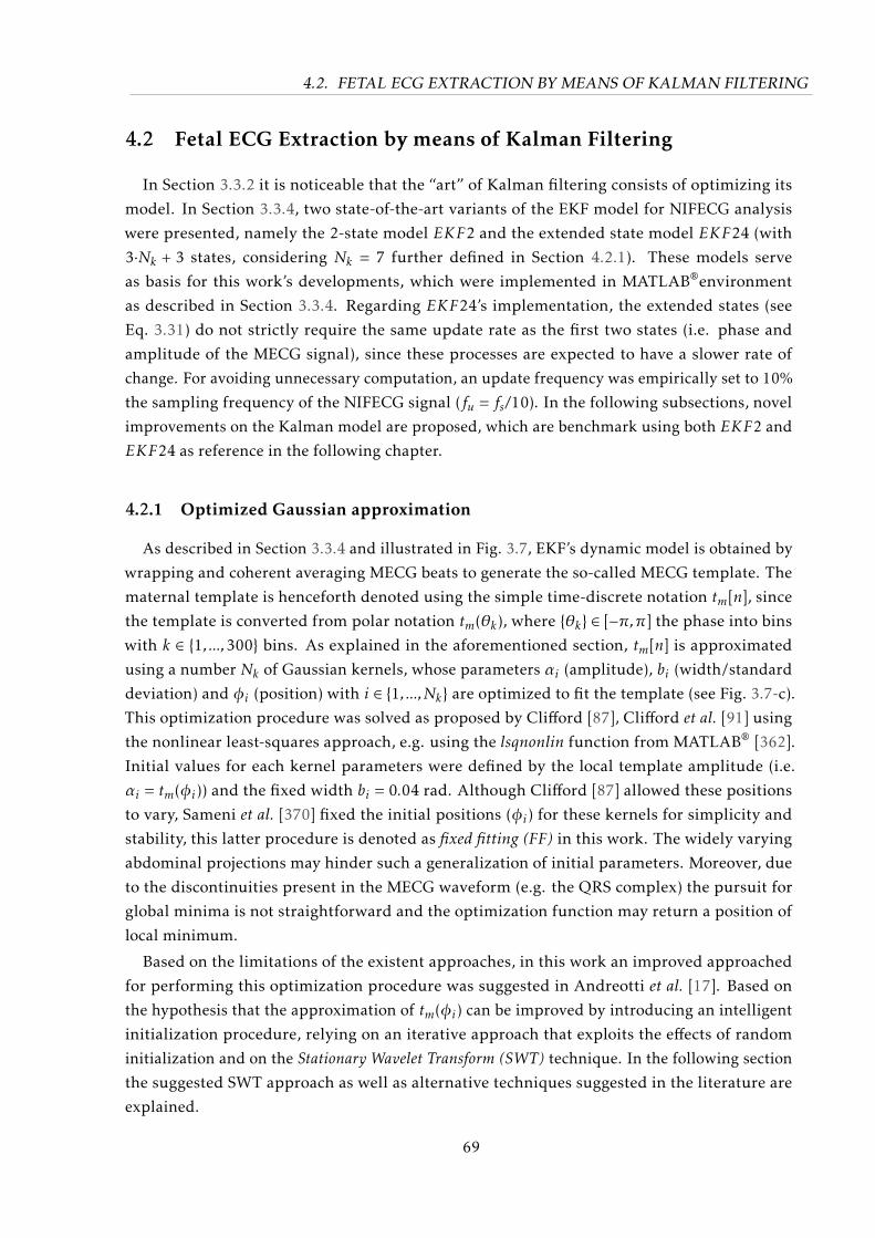
4.2. FETAL ECG EXTRACTION BY MEANS OF KALMAN FILTERING
4.2 Fetal ECG Extraction by means of Kalman Filtering
In Section 3.3.2 it is noticeable that the “art” of Kalman filtering consists of optimizing its
model. In Section 3.3.4, two state-of-the-art variants of the EKF model for NIFECG analysis
were presented, namely the 2-state model EKF2 and the extended state model EKF24 (with
3·Nk + 3 states, considering Nk = 7 further defined in Section 4.2.1). These models serve
as basis for this work’s developments, which were implemented in MATLAB®environment
as described in Section 3.3.4. Regarding EKF24’s implementation, the extended states (see
Eq. 3.31) do not strictly require the same update rate as the first two states (i.e. phase and
amplitude of the MECG signal), since these processes are expected to have a slower rate of
change. For avoiding unnecessary computation, an update frequency was empirically set to 10%
the sampling frequency of the NIFECG signal (fu = fs/10). In the following subsections, novel
improvements on the Kalman model are proposed, which are benchmark using both EKF2 and
EKF24 as reference in the following chapter.
4.2.1 Optimized Gaussian approximation
As described in Section 3.3.4 and illustrated in Fig. 3.7, EKF’s dynamic model is obtained by
wrapping and coherent averaging MECG beats to generate the so-called MECG template. The
maternal template is henceforth denoted using the simple time-discrete notation tm[n], since
the template is converted from polar notation tm(θk), where θk ∈ [−π,π] the phase into bins
with k ∈ 1, ...,300 bins. As explained in the aforementioned section, tm[n] is approximated
using a number Nk of Gaussian kernels, whose parameters αi (amplitude), bi (width/standard
deviation) and φi (position) with i ∈ 1, ...,Nk are optimized to fit the template (see Fig. 3.7-c).
This optimization procedure was solved as proposed by Clifford [87], Clifford et al. [91] using
the nonlinear least-squares approach, e.g. using the lsqnonlin function from MATLAB® [362].
Initial values for each kernel parameters were defined by the local template amplitude (i.e.
αi = tm(φi)) and the fixed width bi = 0.04 rad. Although Clifford [87] allowed these positions
to vary, Sameni et al. [370] fixed the initial positions (φi) for these kernels for simplicity and
stability, this latter procedure is denoted as fixed fitting (FF) in this work. The widely varying
abdominal projections may hinder such a generalization of initial parameters. Moreover, due
to the discontinuities present in the MECG waveform (e.g. the QRS complex) the pursuit for
global minima is not straightforward and the optimization function may return a position of
local minimum.
Based on the limitations of the existent approaches, in this work an improved approached
for performing this optimization procedure was suggested in Andreotti et al. [17]. Based on
the hypothesis that the approximation of tm(φi) can be improved by introducing an intelligent
initialization procedure, relying on an iterative approach that exploits the effects of random
initialization and on the Stationary Wavelet Transform (SWT) technique. In the following section
the suggested SWT approach as well as alternative techniques suggested in the literature are
explained.
69
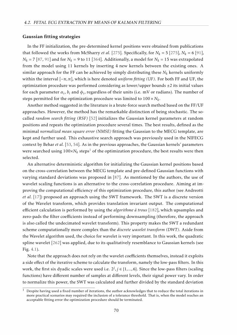
4.2. FETAL ECG EXTRACTION BY MEANS OF KALMAN FILTERING
Gaussian fitting strategies
In the FF initialization, the pre-determined kernel positions were obtained from publications
that followed the works from McSharry et al. [275]. Specifically, for Nk = 5 [275], Nk = 6 [91],
Nk = 7 [87, 91] and for Nk = 9 to 11 [364]. Additionally, a model for Nk = 15 was extrapolated
from the model using 11 kernels by inserting 4 new kernels between the existing ones. A
similar approach for the FF can be achieved by simply distributing these Nk kernels uniformly
within the interval [−π,π], which is here denoted uniform fitting (UF). For both FF and UF, the
optimization procedure was performed considering as lower/upper bounds ±2 its initial values
for each parameter αi , bi and φi , regardless of their units (i.e. mV or radians). The number of
steps permitted for the optimization procedure was limited to 100×Nk .Another method suggested in the literature is a brute-force search method based on the FF/UF
approaches. However, the method has the remarkable distinction of being stochastic. The so-
called random search fitting (RSF) [52] initializes the Gaussian kernel parameters at random
positions and repeats the optimization procedure several times. The best results, defined as the
minimal normalized mean square error (NMSE) fitting the Gaussian to the MECG template, are
kept and further used. This exhaustive search approach was previously used in the NIFECG
context by Behar et al. [53, 54]. As in the previous approaches, the Gaussian kernels’ parameters
were searched using 100×Nk steps1 of the optimization procedure, the best results were then
selected.
An alternative deterministic algorithm for initializing the Gaussian kernel positions based
on the cross-correlation between the MECG template and pre-defined Gaussian functions with
varying standard deviations was proposed in [87]. As mentioned by the authors, the use of
wavelet scaling functions is an alternative to the cross-correlation procedure. Aiming at im-
proving the computational efficiency of this optimization procedure, this author (see Andreotti
et al. [17]) proposed an approach using the SWT framework. The SWT is a discrete version
of the Wavelet transform, which provides translation invariant output. The computational
efficient calculation is performed by using the algorithme à trous [182], which upsamples and
zero-pads the filter coefficients instead of performing downsampling (therefore, the approach
is also called the undecimated wavelet transform). This property makes the SWT a redundant
scheme computationally more complex than the discrete wavelet transform (DWT). Aside from
the Wavelet algorithm used, the choice for wavelet is very important. In this work, the quadratic
spline wavelet [262] was applied, due to its qualitatively resemblance to Gaussian kernels (see
Fig. 4.1).
Note that the approach does not rely on the wavelet coefficients themselves, instead it exploits
a side effect of the iterative scheme to calculate the transform, namely the low-pass filters. In this
work, the first six dyadic scales were used i.e. 2j , j ∈ 1, ...,6. Since the low-pass filters (scaling
functions) have different number of samples at different levels, their signal power vary. In order
to normalize this power, the SWT was calculated and further divided by the standard deviation
1 Despite having used a fixed number of iterations, the author acknowledges that to reduce the total iterations inmore practical scenarios may required the inclusion of a tolerance threshold. That is, when the model reaches anacceptable fitting error the optimization procedure should be terminated.
70
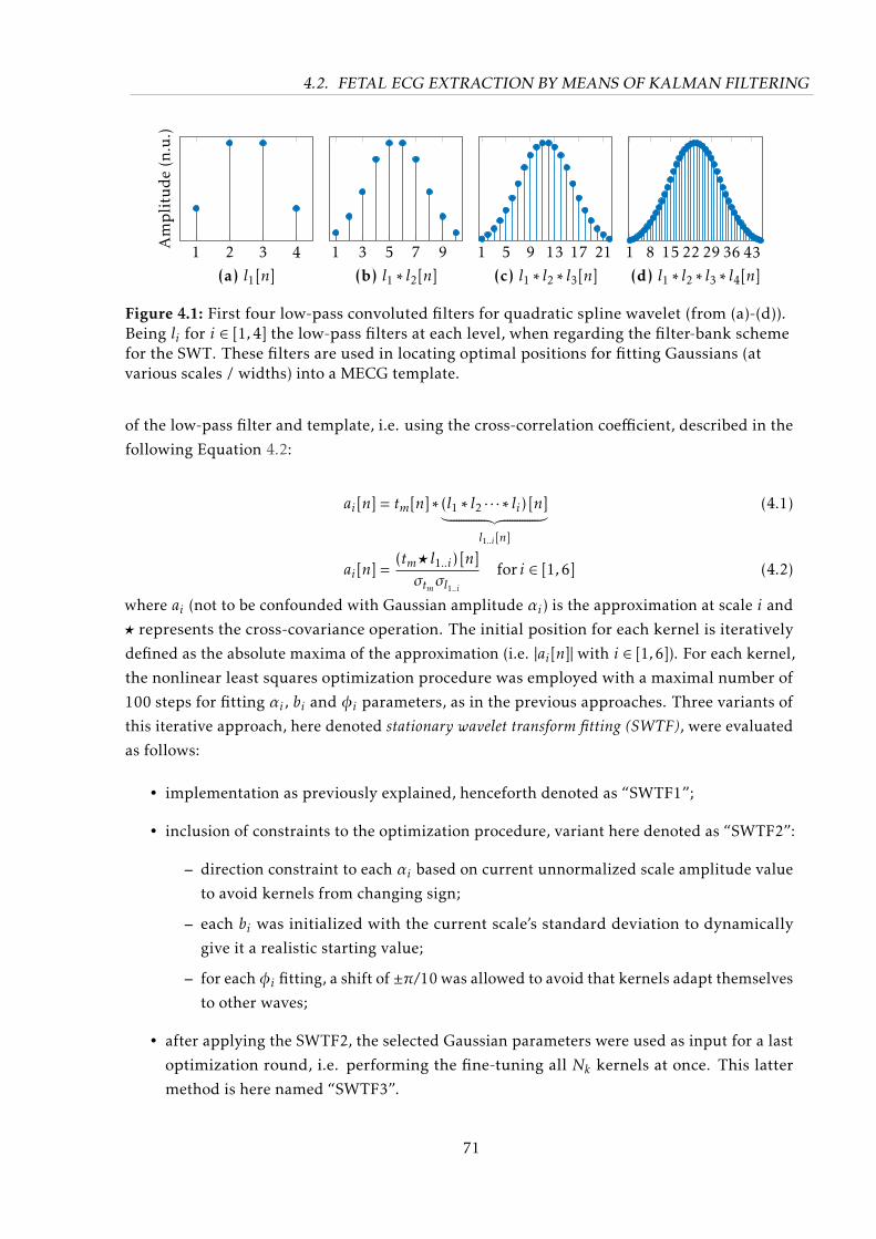
4.2. FETAL ECG EXTRACTION BY MEANS OF KALMAN FILTERING
1 2 3 4(a) l1[n]
Amplitude(n.u.)
1 3 5 7 9(b) l1 ∗ l2[n]
1 5 9 13 17 21(c) l1 ∗ l2 ∗ l3[n]
1 8 15 22 29 36 43(d) l1 ∗ l2 ∗ l3 ∗ l4[n]
Figure 4.1: First four low-pass convoluted filters for quadratic spline wavelet (from (a)-(d)).Being li for i ∈ [1,4] the low-pass filters at each level, when regarding the filter-bank schemefor the SWT. These filters are used in locating optimal positions for fitting Gaussians (atvarious scales / widths) into a MECG template.
of the low-pass filter and template, i.e. using the cross-correlation coefficient, described in the
following Equation 4.2:
ai[n] = tm[n] ∗ (l1 ∗ l2 · · · ∗ li) [n]︸ ︷︷ ︸l1..i [n]
(4.1)
ai[n] =(tm? l1..i) [n]σtmσl1..i
for i ∈ [1,6] (4.2)
where ai (not to be confounded with Gaussian amplitude αi) is the approximation at scale i and
? represents the cross-covariance operation. The initial position for each kernel is iteratively
defined as the absolute maxima of the approximation (i.e. |ai[n]| with i ∈ [1,6]). For each kernel,
the nonlinear least squares optimization procedure was employed with a maximal number of
100 steps for fitting αi , bi and φi parameters, as in the previous approaches. Three variants of
this iterative approach, here denoted stationary wavelet transform fitting (SWTF), were evaluated
as follows:
• implementation as previously explained, henceforth denoted as “SWTF1”;
• inclusion of constraints to the optimization procedure, variant here denoted as “SWTF2”:
– direction constraint to each αi based on current unnormalized scale amplitude value
to avoid kernels from changing sign;
– each bi was initialized with the current scale’s standard deviation to dynamically
give it a realistic starting value;
– for eachφi fitting, a shift of ±π/10 was allowed to avoid that kernels adapt themselves
to other waves;
• after applying the SWTF2, the selected Gaussian parameters were used as input for a last
optimization round, i.e. performing the fine-tuning all Nk kernels at once. This latter
method is here named “SWTF3”.
71
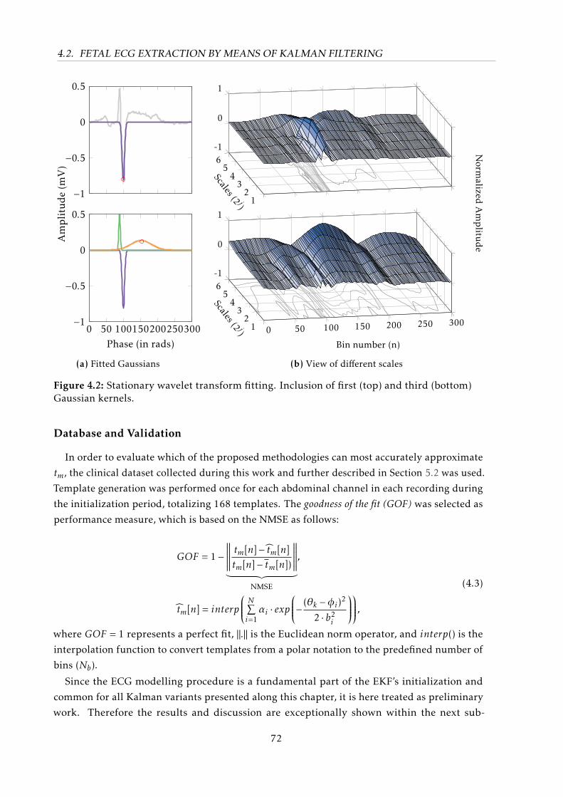
4.2. FETAL ECG EXTRACTION BY MEANS OF KALMAN FILTERING
−1
−0.5
0
0.5
0 50 100150200250300−1
−0.5
0
0.5
Phase (in rads)
Amplitude(m
V)
(a) Fitted Gaussians
12
34
56-1
0
1
Scales (2 j)0 50 100 150 200 250 3001
23
45
6-1
0
1
Bin number (n)Scales (2 j)
Norm
alizedAmplitu
de
(b) View of different scales
Figure 4.2: Stationary wavelet transform fitting. Inclusion of first (top) and third (bottom)Gaussian kernels.
Database and Validation
In order to evaluate which of the proposed methodologies can most accurately approximate
tm, the clinical dataset collected during this work and further described in Section 5.2 was used.
Template generation was performed once for each abdominal channel in each recording during
the initialization period, totalizing 168 templates. The goodness of the fit (GOF) was selected as
performance measure, which is based on the NMSE as follows:
GOF = 1−∥∥∥∥∥∥ tm[n]− tm[n]tm[n]− tm[n])
∥∥∥∥∥∥︸ ︷︷ ︸NMSE
,
tm[n] = interp
N∑i=1αi · exp
− (θk −φi)2
2 · b2i
,(4.3)
where GOF = 1 represents a perfect fit, ‖.‖ is the Euclidean norm operator, and interp() is the
interpolation function to convert templates from a polar notation to the predefined number of
bins (Nb).
Since the ECG modelling procedure is a fundamental part of the EKF’s initialization and
common for all Kalman variants presented along this chapter, it is here treated as preliminary
work. Therefore the results and discussion are exceptionally shown within the next sub-
72
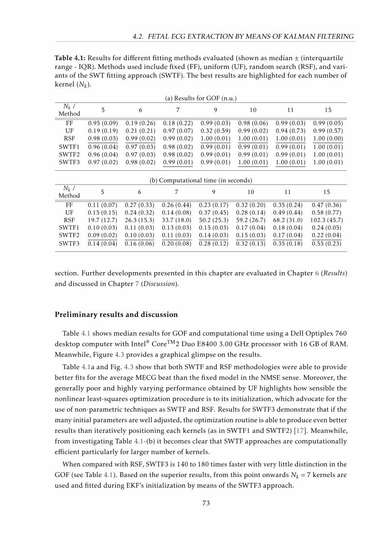
4.2. FETAL ECG EXTRACTION BY MEANS OF KALMAN FILTERING
Table 4.1: Results for different fitting methods evaluated (shown as median ± (interquartilerange - IQR). Methods used include fixed (FF), uniform (UF), random search (RSF), and vari-ants of the SWT fitting approach (SWTF). The best results are highlighted for each number ofkernel (Nk).
(a) Results for GOF (n.u.)Nk /
Method 5 6 7 9 10 11 15
FF 0.95 (0.09) 0.19 (0.26) 0.18 (0.22) 0.99 (0.03) 0.98 (0.06) 0.99 (0.03) 0.99 (0.05)UF 0.19 (0.19) 0.21 (0.21) 0.97 (0.07) 0.32 (0.59) 0.99 (0.02) 0.94 (0.73) 0.99 (0.57)RSF 0.98 (0.03) 0.99 (0.02) 0.99 (0.02) 1.00 (0.01) 1.00 (0.01) 1.00 (0.01) 1.00 (0.00)
SWTF1 0.96 (0.04) 0.97 (0.03) 0.98 (0.02) 0.99 (0.01) 0.99 (0.01) 0.99 (0.01) 1.00 (0.01)SWTF2 0.96 (0.04) 0.97 (0.03) 0.98 (0.02) 0.99 (0.01) 0.99 (0.01) 0.99 (0.01) 1.00 (0.01)SWTF3 0.97 (0.02) 0.98 (0.02) 0.99 (0.01) 0.99 (0.01) 1.00 (0.01) 1.00 (0.01) 1.00 (0.01)
(b) Computational time (in seconds)Nk /
Method 5 6 7 9 10 11 15
FF 0.11 (0.07) 0.27 (0.33) 0.26 (0.44) 0.23 (0.17) 0.32 (0.20) 0.35 (0.24) 0.47 (0.36)UF 0.15 (0.15) 0.24 (0.32) 0.14 (0.08) 0.37 (0.45) 0.28 (0.14) 0.49 (0.44) 0.58 (0.77)RSF 19.7 (12.7) 26.3 (15.3) 33.7 (18.0) 50.2 (25.3) 59.2 (26.7) 68.2 (31.0) 102.3 (45.7)
SWTF1 0.10 (0.03) 0.11 (0.03) 0.13 (0.03) 0.15 (0.03) 0.17 (0.04) 0.18 (0.04) 0.24 (0.05)SWTF2 0.09 (0.02) 0.10 (0.03) 0.11 (0.03) 0.14 (0.03) 0.15 (0.03) 0.17 (0.04) 0.22 (0.04)SWTF3 0.14 (0.04) 0.16 (0.06) 0.20 (0.08) 0.28 (0.12) 0.32 (0.13) 0.35 (0.18) 0.55 (0.23)
section. Further developments presented in this chapter are evaluated in Chapter 6 (Results)and discussed in Chapter 7 (Discussion).
Preliminary results and discussion
Table 4.1 shows median results for GOF and computational time using a Dell Optiplex 760
desktop computer with Intel® CoreTM2 Duo E8400 3.00 GHz processor with 16 GB of RAM.
Meanwhile, Figure 4.3 provides a graphical glimpse on the results.
Table 4.1a and Fig. 4.3 show that both SWTF and RSF methodologies were able to provide
better fits for the average MECG beat than the fixed model in the NMSE sense. Moreover, the
generally poor and highly varying performance obtained by UF highlights how sensible the
nonlinear least-squares optimization procedure is to its initialization, which advocate for the
use of non-parametric techniques as SWTF and RSF. Results for SWTF3 demonstrate that if the
many initial parameters are well adjusted, the optimization routine is able to produce even better
results than iteratively positioning each kernels (as in SWTF1 and SWTF2) [17]. Meanwhile,
from investigating Table 4.1-(b) it becomes clear that SWTF approaches are computationally
efficient particularly for larger number of kernels.
When compared with RSF, SWTF3 is 140 to 180 times faster with very little distinction in the
GOF (see Table 4.1). Based on the superior results, from this point onwards Nk = 7 kernels are
used and fitted during EKF’s initialization by means of the SWTF3 approach.
73
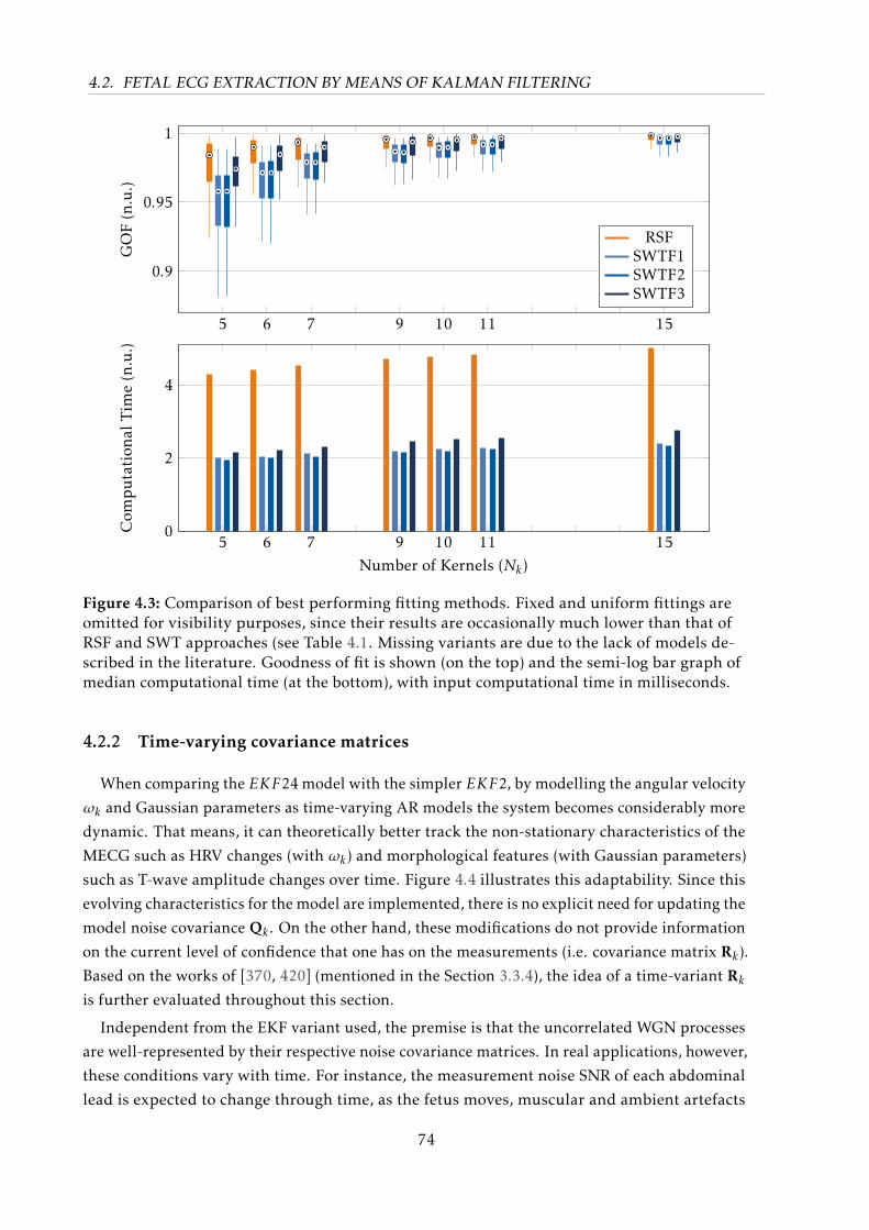
4.2. FETAL ECG EXTRACTION BY MEANS OF KALMAN FILTERING
5 6 7 9 10 11 15
0.9
0.95
1GOF(n.u.)
RSFSWTF1SWTF2SWTF3
5 6 7 9 10 11 150
2
4
Number of Kernels (Nk)
Com
putation
alTim
e(n.u.)
Figure 4.3: Comparison of best performing fitting methods. Fixed and uniform fittings areomitted for visibility purposes, since their results are occasionally much lower than that ofRSF and SWT approaches (see Table 4.1. Missing variants are due to the lack of models de-scribed in the literature. Goodness of fit is shown (on the top) and the semi-log bar graph ofmedian computational time (at the bottom), with input computational time in milliseconds.
4.2.2 Time-varying covariance matrices
When comparing the EKF24 model with the simpler EKF2, by modelling the angular velocity
ωk and Gaussian parameters as time-varying AR models the system becomes considerably more
dynamic. That means, it can theoretically better track the non-stationary characteristics of the
MECG such as HRV changes (with ωk) and morphological features (with Gaussian parameters)
such as T-wave amplitude changes over time. Figure 4.4 illustrates this adaptability. Since this
evolving characteristics for the model are implemented, there is no explicit need for updating the
model noise covariance Qk . On the other hand, these modifications do not provide information
on the current level of confidence that one has on the measurements (i.e. covariance matrix Rk).
Based on the works of [370, 420] (mentioned in the Section 3.3.4), the idea of a time-variant Rkis further evaluated throughout this section.
Independent from the EKF variant used, the premise is that the uncorrelated WGN processes
are well-represented by their respective noise covariance matrices. In real applications, however,
these conditions vary with time. For instance, the measurement noise SNR of each abdominal
lead is expected to change through time, as the fetus moves, muscular and ambient artefacts
74
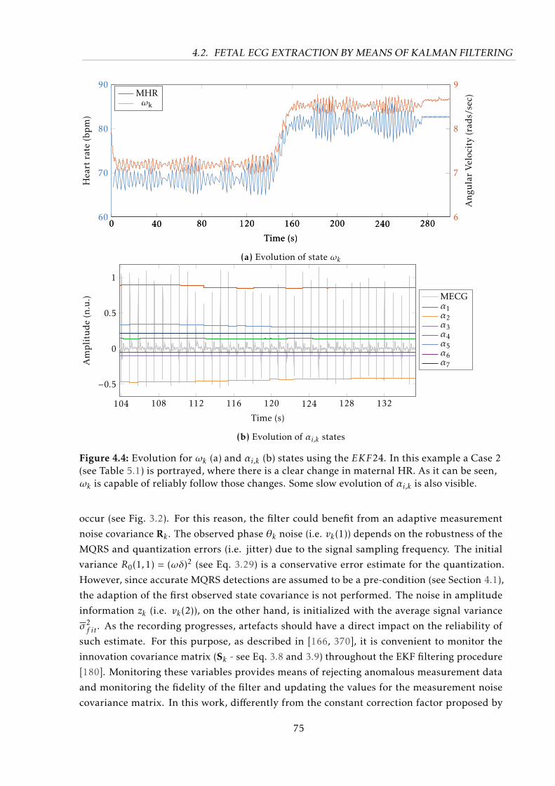
4.2. FETAL ECG EXTRACTION BY MEANS OF KALMAN FILTERING
0 40 80 120 160 200 240 28060
70
80
90
Time (s)
Heart
rate
(bpm)
0 40 80 120 160 200 240 2806
7
8
9
Time (s)
Ang
ularVelocity(rad
s/sec)
MHRωk
(a) Evolution of state ωk
104 108 112 116 120 124 128 132
−0.5
0
0.5
1
Time (s)
Amplitude(n.u.) MECG
α1α2α3α4α5α6α7
(b) Evolution of αi,k states
Figure 4.4: Evolution for ωk (a) and αi,k (b) states using the EKF24. In this example a Case 2(see Table 5.1) is portrayed, where there is a clear change in maternal HR. As it can be seen,ωk is capable of reliably follow those changes. Some slow evolution of αi,k is also visible.
occur (see Fig. 3.2). For this reason, the filter could benefit from an adaptive measurement
noise covariance Rk . The observed phase θk noise (i.e. vk(1)) depends on the robustness of the
MQRS and quantization errors (i.e. jitter) due to the signal sampling frequency. The initial
variance R0(1,1) = (ωδ)2 (see Eq. 3.29) is a conservative error estimate for the quantization.
However, since accurate MQRS detections are assumed to be a pre-condition (see Section 4.1),
the adaption of the first observed state covariance is not performed. The noise in amplitude
information zk (i.e. vk(2)), on the other hand, is initialized with the average signal variance
σ2f it. As the recording progresses, artefacts should have a direct impact on the reliability of
such estimate. For this purpose, as described in [166, 370], it is convenient to monitor the
innovation covariance matrix (Sk - see Eq. 3.8 and 3.9) throughout the EKF filtering procedure
[180]. Monitoring these variables provides means of rejecting anomalous measurement data
and monitoring the fidelity of the filter and updating the values for the measurement noise
covariance matrix. In this work, differently from the constant correction factor proposed by
75

4.2. FETAL ECG EXTRACTION BY MEANS OF KALMAN FILTERING
Sameni et al. [370], a correction is applied only in cases when the innovation covariance exceeds
a given confidence interval as further shown.
As explained in Section 3.3.2, on the linear case the innovation is a random, zero-mean
and Gaussian distributed variable, which should be independent and white as long as the KF
properly works [277] (for EKF this is only marginally true). If that is the case, Sk (from Eq. 3.9
should match the true innovation covariance matrix, i.e. σ2S,k = E[νk(2)·νk(2)T ]. If this is not
true, considering Eq. 3.9 it can be concluded that either Pk|k−1, H or Rk does not represent the
system anymore. Since several improvements to the EKF model took place as demonstrated on
the previous chapter, it can be assumed that Rk (i.e. R0 for the invariant case) is the cause for
such mismatch. An online adaptation for rk (i.e. noise relative to zk , following the notation from
Section 3.3.4) is attained from Eq. 3.9 as [180, 277]:
rk = σ2S,k − h·pk|k−1·hT , (4.4)
where h represents the second row of the observational matrixH and pk|k−1 is the second element
on the main diagonal of Pk|k−1. Assuming that the innovation νk ∼N (0,Sk), one can empirically
estimate the true innovation variance as the sample variance S2 [180, 277, 307]:
S2 =1
L− 1
k−L∑i=k
(νi(2)−E[νi(2)])2 =1
L− 1
k−1∑i=k−L
ν2i (2), (4.5)
where the L is the number of samples that should be averaged. S2 is a random variable, whose
sampling distribution follows a Chi-square distribution (S2(L−1)/Sk(2,2) ∼ χ2L−1). Therefore, while
updating rk (in Eq. 4.4), it is important to make sure that the empirical value S2 has values
outside a given confidence interval (CI), i.e. it is very probable that E[S2
], h·pk|k−1·hT . In this
work a 99% CI is used, in case the empirical variance exceeds these limits rk shall be updated.
The CI for the χ2 distribution with L degrees of freedom, is given by [180]:
CI =
L · S2
χ21− α2 ,L
,L · S2
χ2α2 ,L
. (4.6)
The specified χ2 quantiles are obtained based on [180] as:
χ21− α2 ;L = 0.5(
√2L− 1 + 2.58)2, (4.7)
χ2α2 ;L = 0.5(
√2L− 1− 2.58)2. (4.8)
An implementation detail is the definition for the value L. This window length should make
sure that it represents actual SNR changes and not physiological changes on the MECG signal
amplitude, e.g. due to shift of the cardiac vector during respiration. For this reason, in this work
L was empirically set to comprise 10 MECG cycles [180], i.e. L = 10 · (2π·fs/ωk). Moreover, the
changes in the rk process are expected to be slower than the EKF filter. For avoiding unnecessary
computational effort, rk is updated with a frequency that equals 10% the signal’s sampling
frequency, similarly to the extended state update in EKF24 variant previously mentioned. In
76
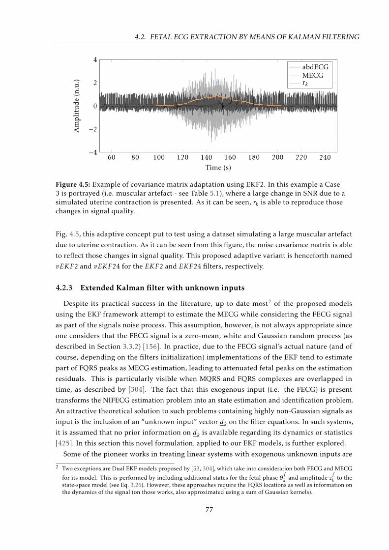
4.2. FETAL ECG EXTRACTION BY MEANS OF KALMAN FILTERING
60 80 100 120 140 160 180 200 220 240−4
−2
0
2
4
Time (s)
Amplitude(n.u.)
abdECGMECGrk
Figure 4.5: Example of covariance matrix adaptation using EKF2. In this example a Case3 is portrayed (i.e. muscular artefact - see Table 5.1), where a large change in SNR due to asimulated uterine contraction is presented. As it can be seen, rk is able to reproduce thosechanges in signal quality.
Fig. 4.5, this adaptive concept put to test using a dataset simulating a large muscular artefact
due to uterine contraction. As it can be seen from this figure, the noise covariance matrix is able
to reflect those changes in signal quality. This proposed adaptive variant is henceforth named
vEKF2 and vEKF24 for the EKF2 and EKF24 filters, respectively.
4.2.3 Extended Kalman filter with unknown inputs
Despite its practical success in the literature, up to date most2 of the proposed models
using the EKF framework attempt to estimate the MECG while considering the FECG signal
as part of the signals noise process. This assumption, however, is not always appropriate since
one considers that the FECG signal is a zero-mean, white and Gaussian random process (as
described in Section 3.3.2) [156]. In practice, due to the FECG signal’s actual nature (and of
course, depending on the filters initialization) implementations of the EKF tend to estimate
part of FQRS peaks as MECG estimation, leading to attenuated fetal peaks on the estimation
residuals. This is particularly visible when MQRS and FQRS complexes are overlapped in
time, as described by [304]. The fact that this exogenous input (i.e. the FECG) is present
transforms the NIFECG estimation problem into an state estimation and identification problem.
An attractive theoretical solution to such problems containing highly non-Gaussian signals as
input is the inclusion of an “unknown input” vector dk on the filter equations. In such systems,
it is assumed that no prior information on dk is available regarding its dynamics or statistics
[425]. In this section this novel formulation, applied to our EKF models, is further explored.
Some of the pioneer works in treating linear systems with exogenous unknown inputs are
2 Two exceptions are Dual EKF models proposed by [53, 304], which take into consideration both FECG and MECG
for its model. This is performed by including additional states for the fetal phase θfk and amplitude z
fk to the
state-space model (see Eq. 3.26). However, these approaches require the FQRS locations as well as information onthe dynamics of the signal (on those works, also approximated using a sum of Gaussian kernels).
77
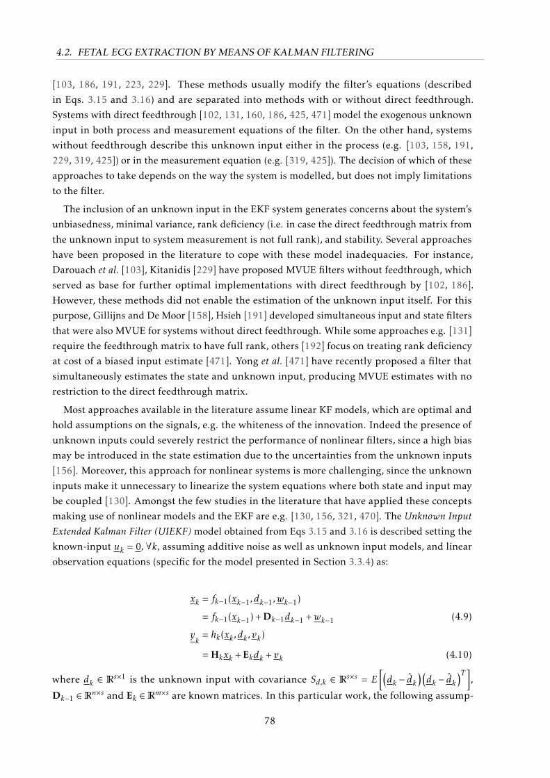
4.2. FETAL ECG EXTRACTION BY MEANS OF KALMAN FILTERING
[103, 186, 191, 223, 229]. These methods usually modify the filter’s equations (described
in Eqs. 3.15 and 3.16) and are separated into methods with or without direct feedthrough.
Systems with direct feedthrough [102, 131, 160, 186, 425, 471] model the exogenous unknown
input in both process and measurement equations of the filter. On the other hand, systems
without feedthrough describe this unknown input either in the process (e.g. [103, 158, 191,
229, 319, 425]) or in the measurement equation (e.g. [319, 425]). The decision of which of these
approaches to take depends on the way the system is modelled, but does not imply limitations
to the filter.
The inclusion of an unknown input in the EKF system generates concerns about the system’s
unbiasedness, minimal variance, rank deficiency (i.e. in case the direct feedthrough matrix from
the unknown input to system measurement is not full rank), and stability. Several approaches
have been proposed in the literature to cope with these model inadequacies. For instance,
Darouach et al. [103], Kitanidis [229] have proposed MVUE filters without feedthrough, which
served as base for further optimal implementations with direct feedthrough by [102, 186].
However, these methods did not enable the estimation of the unknown input itself. For this
purpose, Gillijns and De Moor [158], Hsieh [191] developed simultaneous input and state filters
that were also MVUE for systems without direct feedthrough. While some approaches e.g. [131]
require the feedthrough matrix to have full rank, others [192] focus on treating rank deficiency
at cost of a biased input estimate [471]. Yong et al. [471] have recently proposed a filter that
simultaneously estimates the state and unknown input, producing MVUE estimates with no
restriction to the direct feedthrough matrix.
Most approaches available in the literature assume linear KF models, which are optimal and
hold assumptions on the signals, e.g. the whiteness of the innovation. Indeed the presence of
unknown inputs could severely restrict the performance of nonlinear filters, since a high bias
may be introduced in the state estimation due to the uncertainties from the unknown inputs
[156]. Moreover, this approach for nonlinear systems is more challenging, since the unknown
inputs make it unnecessary to linearize the system equations where both state and input may
be coupled [130]. Amongst the few studies in the literature that have applied these concepts
making use of nonlinear models and the EKF are e.g. [130, 156, 321, 470]. The Unknown InputExtended Kalman Filter (UIEKF) model obtained from Eqs 3.15 and 3.16 is described setting the
known-input uk = 0, ∀k, assuming additive noise as well as unknown input models, and linear
observation equations (specific for the model presented in Section 3.3.4) as:
xk = fk−1(xk−1,dk−1,wk−1)
= fk−1(xk−1) + Dk−1dk−1 +wk−1 (4.9)
yk
= hk(xk ,dk ,vk)
= Hkxk + Ekdk + vk (4.10)
where dk ∈ Rs×1 is the unknown input with covariance Sd,k ∈ Rs×s = E[(dk − dk
)(dk − dk
)T ],
Dk−1 ∈Rn×s and Ek ∈Rm×s are known matrices. In this particular work, the following assump-
78
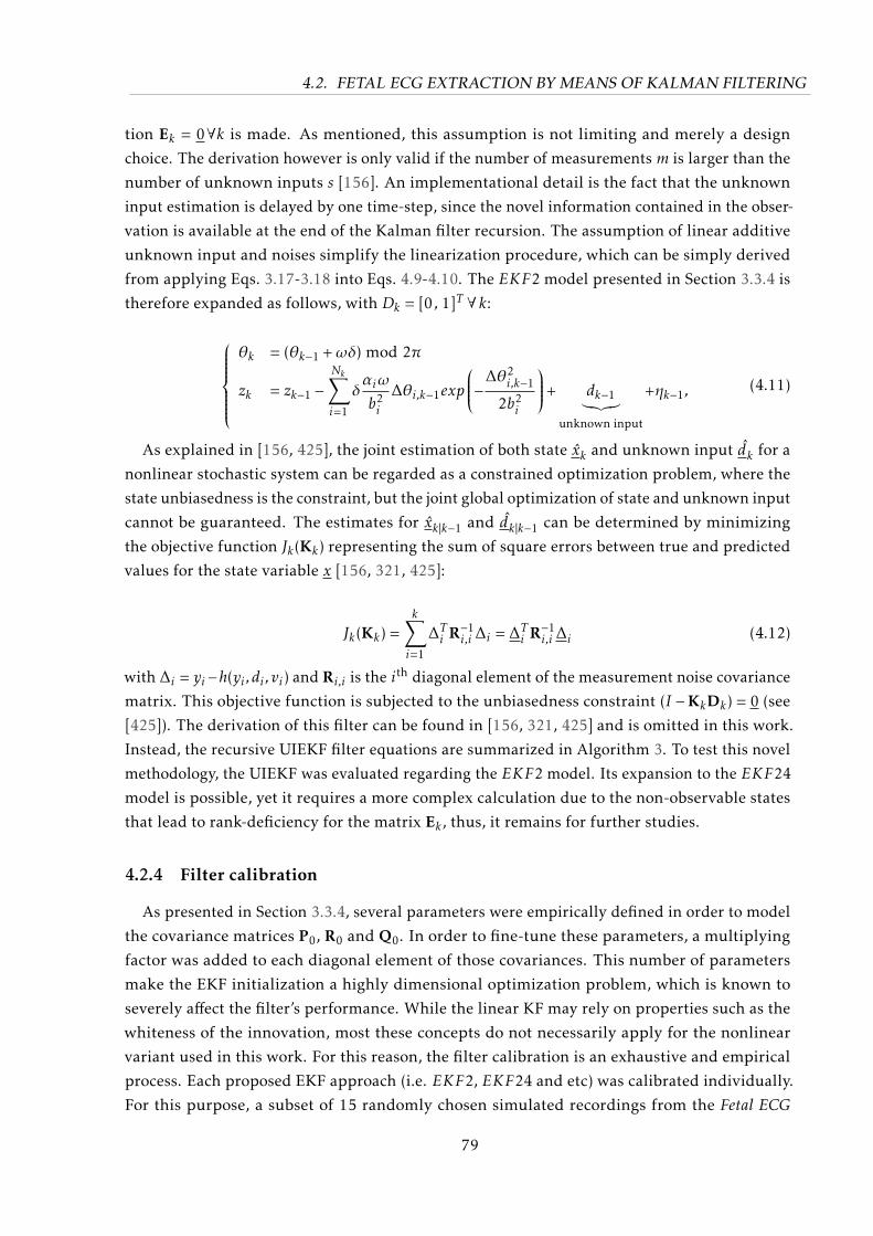
4.2. FETAL ECG EXTRACTION BY MEANS OF KALMAN FILTERING
tion Ek = 0∀k is made. As mentioned, this assumption is not limiting and merely a design
choice. The derivation however is only valid if the number of measurements m is larger than the
number of unknown inputs s [156]. An implementational detail is the fact that the unknown
input estimation is delayed by one time-step, since the novel information contained in the obser-
vation is available at the end of the Kalman filter recursion. The assumption of linear additive
unknown input and noises simplify the linearization procedure, which can be simply derived
from applying Eqs. 3.17-3.18 into Eqs. 4.9-4.10. The EKF2 model presented in Section 3.3.4 is
therefore expanded as follows, with Dk = [0 , 1]T ∀k:
θk = (θk−1 +ωδ) mod 2π
zk = zk−1 −Nk∑i=1
δαiω
b2i
∆θi,k−1exp
−∆θ2i,k−1
2b2i
+ dk−1︸︷︷︸unknown input
+ηk−1, (4.11)
As explained in [156, 425], the joint estimation of both state xk and unknown input dk for a
nonlinear stochastic system can be regarded as a constrained optimization problem, where the
state unbiasedness is the constraint, but the joint global optimization of state and unknown input
cannot be guaranteed. The estimates for xk|k−1 and dk|k−1 can be determined by minimizing
the objective function Jk(Kk) representing the sum of square errors between true and predicted
values for the state variable x [156, 321, 425]:
Jk(Kk) =k∑i=1
∆Ti R−1i,i ∆i = ∆Ti R−1
i,i ∆i (4.12)
with ∆i = yi−h(yi ,di ,vi) and Ri,i is the ith diagonal element of the measurement noise covariance
matrix. This objective function is subjected to the unbiasedness constraint (I −KkDk) = 0 (see
[425]). The derivation of this filter can be found in [156, 321, 425] and is omitted in this work.
Instead, the recursive UIEKF filter equations are summarized in Algorithm 3. To test this novel
methodology, the UIEKF was evaluated regarding the EKF2 model. Its expansion to the EKF24
model is possible, yet it requires a more complex calculation due to the non-observable states
that lead to rank-deficiency for the matrix Ek , thus, it remains for further studies.
4.2.4 Filter calibration
As presented in Section 3.3.4, several parameters were empirically defined in order to model
the covariance matrices P0, R0 and Q0. In order to fine-tune these parameters, a multiplying
factor was added to each diagonal element of those covariances. This number of parameters
make the EKF initialization a highly dimensional optimization problem, which is known to
severely affect the filter’s performance. While the linear KF may rely on properties such as the
whiteness of the innovation, most these concepts do not necessarily apply for the nonlinear
variant used in this work. For this reason, the filter calibration is an exhaustive and empirical
process. Each proposed EKF approach (i.e. EKF2, EKF24 and etc) was calibrated individually.
For this purpose, a subset of 15 randomly chosen simulated recordings from the Fetal ECG
79

4.2. FETAL ECG EXTRACTION BY MEANS OF KALMAN FILTERING
Algorithm 3 Pseudo-code summarizing the Unknown Input Extended Kalman Filter algorithm(time and measurement-update form)Require: models for Ak ,Hk , Qk , RkInitialize: x0, P0for k = 1 to Nsamples do
// Prediction step
Fk−1 ≈ ∂fk−1∂xk−1
∣∣∣∣wk−1=0xk−1=xk−1|k−1
and Wk−1 ≈ ∂fk−1∂w
∣∣∣∣wk−1=0xk−1=xk−1|k−1
; // linearization
xk|k−1 = Fk−1xk−1|k−1 + Dk−1dk−1|k−2 ; // a priori state estimate
Pk|k−1 = Fk−1Pk−1|k−1FTk−1 + Wk−1Qk−1WTk ; // a priori covariance estimate
// Update stepνk = y
k− hk(xk|k−1,0) ; // innovation signal
Sk = HkPk|k−1HTk + Rk ; // innovation covariance
Sd,k =[DkHkR−1
k
(I−HT
k Kk
)HkDk
]−1; // unknown input covariance
Kk = Pk|k−1HTk S−1
k ; // obtain Kalman gain
xk|k = xk|k−1 + Kkνk ; // a posteriori state estimate
dk−1|k = Sd,kDTk HT
k R−1k
[(I−HT
k Kk
)(νk + HT
k Dk−1dk−2|k−1
)]; // unknown input estimate
Pk|k = (I −KkHk)[Pk|k−1 + Dk−1SkDT
k−1 (I −KkHk)T]
end
Synthetic Database (FECGSYNDB) was used. A random search3 was carried out in attempting to
minimize a multiobjective cost function comprising the following three subfunctions:
This fitting problem is similar to the problem presented in Section 4.2.1, for this reason the
GOF was also used.
MECG residuals: effectively, the EKF attempts to estimate the maternal ECG signal. In order
to assess the quality of EKF’s MECG estimation, the NMSE between estimated and true
maternal signal (available for simulated data) was evaluated. The NMSE was calculated
only within a ±50 ms window around each MQRS complex, excluding segments were
FQRS and MQRS overlaps occurred.
FECG estimation: analogously to the previous metric, while estimating the MECG, the FECG
should not be confounded with the MECG, i.e. the filter should not completely trust the
observed signal. For this purpose, the NMSE difference between the estimation residual
(or unknown input in the uiEKF2 case) and the true fetal signal (available in simulated
data) was evaluated around a ±25 ms of each FQRS complex.
FQRS detection accuracy: this last metric is what one in fact aims to improve, namely the
accuracy of the FQRS detections. This was done by using a simple maxima search FQRS
detector [363] and the F1 metric (see Section 3.4.2) over each extracted signal.
The global cost function consisted of a weighted average of these aforementioned subfunctions
by using weights from 1 to 3 to MECG residuals, FECG estimation and FQRS detection accuracy,
3 The EKF extraction is a computationally expensive operation. Random search algorithms enable the search forhyper-parameters in an efficient manner, compared to grid search algorithms. [60]
80
4.3. ACCURATE FETAL QRS AND HEART RATE DETECTION
respectively. These weights were arbitrarily chosen to reflect the importance of each subfunction
on the extraction result. The set of parameters which at last delivered more often the best results
was used.
4.3 Accurate Fetal QRS and Heart Rate Detection
The increasing interest in NIFECG analysis culminated on PCINCC 2013 [92], which dealt
with the accuracy of FQRS detections and FHR estimates. Indeed, reliable FQRS/FHR estimates
are crucial for the further clinical analysis of NIFECG (e.g. FHR variability or morphological
analysis signal). During the PCINC 2013, various approaches for improving fetal heart rate
detection were presented e.g. [20, 54, 447]. While most available FQRS detection methods are
simple re-parametrized single-channel adult QRS detectors (as described in Section 3.4), FHR
estimates are often based on heuristic rules for how a smooth FHR tracing should appear. The
lack of a general framework impede the understanding and hamper these method’s further
use. Aiming at improving the accuracy of FQRS detections obtain from those simple detection
algorithms, two multichannel correction frameworks are proposed in this work. For this purpose,
the following input signals are assumed to be available:
(i) at least one maternal chest lead;
(ii) reliable MQRS detection/annotation;
(iii) multiple channels of abdominal signals;
(iv) extracted FECG signals from (iii);
(v) initial FQRS detections for each channel.
The two correction methods have substantially distinct characteristics and aim at different
applications. Nonetheless, both algorithms are based on the common idea of applying novel SQI
measures in FECG analysis. In Section 4.3.1, an offline, stochastic approach is presented, which
exhaustively searches for a global solution to the detection problem. The method considers
multiple SQIs as cost functions, requiring a SQI value for each individual FQRS candidate. The
second approach (shown in Section 4.3.2), focuses on real-time applications and is an online,
deterministic and window-based method. For this method a large variety of SQI metrics are
proposed and accordingly evaluated.
4.3.1 Multichannel evolutionary QRS correction
The multichannel method presented in this section was developed at the IBMT by this author
[20, 21] and obtained the highest FQRS detection accuracy scores at the PCINC 2013, regarding
the scoring metrics E1/E4 and E2/E5, amongst all participants. The method was developed in
the scope of a side project in the student research from Himmelsbach [179]. The identification
of fetal peaks on extracted signals is challenging, due to the low SNR of the FECG as well as the
81
4.3. ACCURATE FETAL QRS AND HEART RATE DETECTION
presence of MECG residuals (mainly MQRS complexes), which can easily be confounded with
the FQRS. In order to cope with such demanding task, this novel method makes use of basic
concepts from evolutionary algorithms (EA)4. Due to its origins in evolutionary computing, the
algorithm is henceforth named evolutionary QRS correction algorithm (eQRS).
In EAs artificial individuals are used to populate the search space, through selection, mutationand recombination the population evolves towards optimal regions of the search space. The
recombination mechanism allows the mixing of parental characteristics to be passed to their
descendants and mutation introduces innovation into the population [43]. In our application,
FQRS detections were treated as individuals, where on each iteration FQRS candidates were
allowed to originate, change location or cease existence. That is, although the proposed approach
inherits characteristics from EA that involve randomness, it does not perform a whole-circuit
optimization. Particularly, recombination and mutation are not present due to the lack of
suitable interpretation for such concepts in our application. Although EA’s population is often
arbitrarily initialized [43], for the purpose of faster convergence the start our method with
initial FQRS detections provided by a simple QRS algorithm applied to each channel.
According to Bäck and Schwefel [43], the environment delivers the quality information (i.e.
fitness value (FV) – denoted as FVt,i , being fitness value for individual i at iteration time-step t)
about the search points. The selection process then favors those individuals with higher fitness
to reproduce more often than those of lower fitness. On our FECG application, FVs describe
how well a certain FQRS suits the extracted fetal signal (environment). In order to evaluate
FV values for each individual, particularly designed fetal SQIs are proposed. This global SQI
metric was composed by multiple real-valued objective functions, which can be divided into
two groups based on their features: the FQRS pseudo-periodicity and FECG beat morphology.
These sub-functions can be thought of as different SQI metrics that exploit the morphological
characteristics or regularity of the candidate fetal peaks. The first group of the fitness function,
i.e. morphological features, can not be described by one single feature signal due to the presence
multiple noise sources (e.g. MECG and muscular noises). In order to assess FECG morphology,
two sub-functions were used, namely conformity (cSQI) and extravagance (xSQI). The latter
group of SQI functions is described by a single function that involves the plausibility of the
FHR trace (henceforth called gSQI). A summary on those newly developed SQIs follows:
cSQI measures how conform the FECG complexes are in relation to an coherent averaged FECG
template. This FECG template is created based on the current FQRS location candidates.
By simply taking the correlation coefficient between the averaged template and each
cycle i (centered at the FQRS occurrences), a value in the interval [0,1] is obtained for
each individual. In other words, conformity portraits how similar each individual is to a
4 Evolutionary algorithms are a class of approaches based on biological evolution, as Charles Darwin [104] describedthe “survival of the fittest”. Generic algorithms and EA have various similarities and were proposed by the groupsof John Holland and Hans-Paul Schwefel, respectively [462]. The reader is referred to [43, 462] for generaloverviews. In contrast to traditional algorithms for optimization, EAs are working with probabilistic rules therebyenabling parallel solutions. EAs have become a popular heuristic near-optimal solution for problems with largesearch spaces [462]. Due to the lack of boundaries in creating the global cost function, EAs can be applied in aneasy and flexible way [338].
82
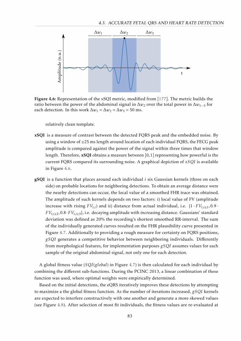
4.3. ACCURATE FETAL QRS AND HEART RATE DETECTION
t
∆w1 ∆w2 ∆w3
Am
pli
tud
e(n
.u.)
Figure 4.6: Representation of the xSQI metric, modified from [177]. The metric builds theratio between the power of the abdominal signal in ∆w2 over the total power in ∆w1···3 foreach detection. In this work ∆w1 = ∆w2 = ∆w3 = 50 ms.
relatively clean template.
xSQI is a measure of contrast between the detected FQRS peak and the embedded noise. By
using a window of ±25 ms length around location of each individual FQRS, the FECG peak
amplitude is compared against the power of the signal within three times that window
length. Therefore, xSQI obtains a measure between [0,1] representing how powerful is the
current FQRS compared its surrounding noise. A graphical depiction of xSQI is available
in Figure 4.6.
gSQI is a function that places around each individual i six Gaussian kernels (three on each
side) on probable locations for neighboring detections. To obtain an average distance were
the nearby detections can occur, the local value of a smoothed FHR trace was obtained.
The amplitude of such kernels depends on two factors: i) local value of FV (amplitude
increase with rising FVt,i) and ii) distance from actual individual, i.e. 1 · FVt,i±1,0.9 ·FVt,i±2,0.8 ·FVt,i±3, i.e. decaying amplitude with increasing distance. Gaussians’ standard
deviation was defined as 20% the recording’s shortest smoothed RR-interval. The sum
of the individually generated curves resulted on the FHR plausibility curve presented in
Figure 4.7. Additionally to providing a rough measure for certainty on FQRS positions,
gSQI generates a competitive behavior between neighboring individuals. Differently
from morphological features, for implementation purposes gSQI assumes values for each
sample of the original abdominal signal, not only one for each detection.
A global fitness value (SQI(global) in Figure 4.7) is then calculated for each individual by
combining the different sub-functions. During the PCINC 2013, a linear combination of these
function was used, where optimal weights were empirically determined.
Based on the initial detections, the eQRS iteratively improves these detections by attempting
to maximize a the global fitness function. As the number of iterations increased, gSQI kernels
are expected to interfere constructively with one another and generate a more skewed values
(see Figure 4.8). After selection of most fit individuals, the fitness values are re-evaluated at
83
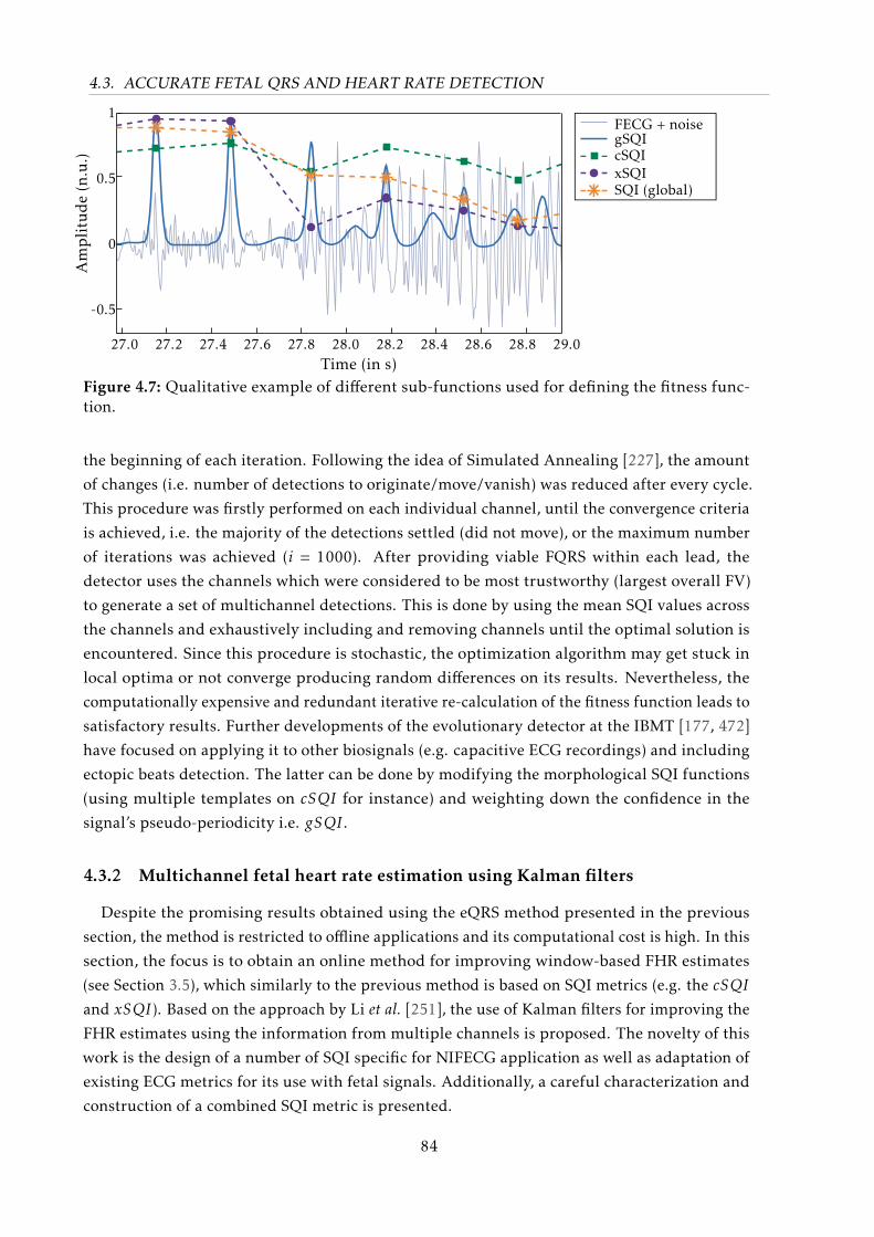
4.3. ACCURATE FETAL QRS AND HEART RATE DETECTION
FECG + noisegSQIcSQIxSQISQI (global)
1
0.5
0
-0.5
27.0 27.2 27.4 27.6 27.8 28.0 28.2 28.4 28.6 28.8 29.0Time (in s)
Am
pli
tud
e(n
.u.)
Figure 4.7: Qualitative example of different sub-functions used for defining the fitness func-tion.
the beginning of each iteration. Following the idea of Simulated Annealing [227], the amount
of changes (i.e. number of detections to originate/move/vanish) was reduced after every cycle.
This procedure was firstly performed on each individual channel, until the convergence criteria
is achieved, i.e. the majority of the detections settled (did not move), or the maximum number
of iterations was achieved (i = 1000). After providing viable FQRS within each lead, the
detector uses the channels which were considered to be most trustworthy (largest overall FV)
to generate a set of multichannel detections. This is done by using the mean SQI values across
the channels and exhaustively including and removing channels until the optimal solution is
encountered. Since this procedure is stochastic, the optimization algorithm may get stuck in
local optima or not converge producing random differences on its results. Nevertheless, the
computationally expensive and redundant iterative re-calculation of the fitness function leads to
satisfactory results. Further developments of the evolutionary detector at the IBMT [177, 472]
have focused on applying it to other biosignals (e.g. capacitive ECG recordings) and including
ectopic beats detection. The latter can be done by modifying the morphological SQI functions
(using multiple templates on cSQI for instance) and weighting down the confidence in the
signal’s pseudo-periodicity i.e. gSQI .
4.3.2 Multichannel fetal heart rate estimation using Kalman filters
Despite the promising results obtained using the eQRS method presented in the previous
section, the method is restricted to offline applications and its computational cost is high. In this
section, the focus is to obtain an online method for improving window-based FHR estimates
(see Section 3.5), which similarly to the previous method is based on SQI metrics (e.g. the cSQI
and xSQI). Based on the approach by Li et al. [251], the use of Kalman filters for improving the
FHR estimates using the information from multiple channels is proposed. The novelty of this
work is the design of a number of SQI specific for NIFECG application as well as adaptation of
existing ECG metrics for its use with fetal signals. Additionally, a careful characterization and
construction of a combined SQI metric is presented.
84
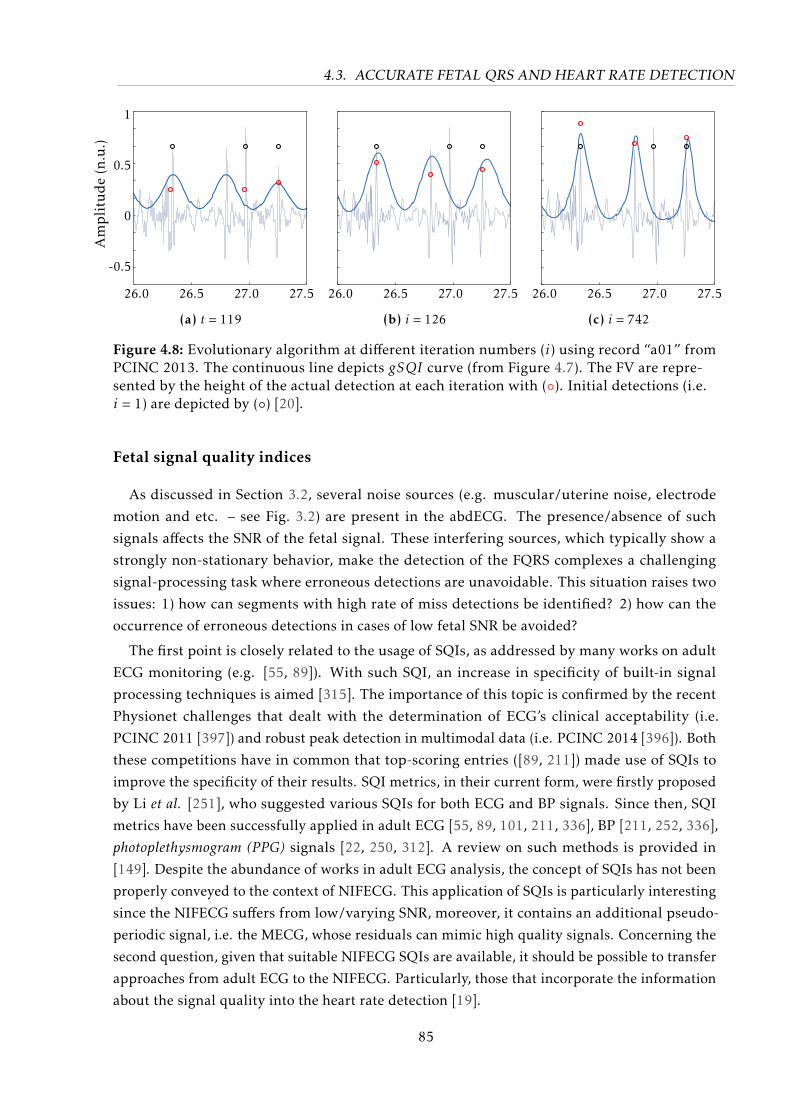
4.3. ACCURATE FETAL QRS AND HEART RATE DETECTION
Am
pli
tud
e(n
.u.)
1
0.5
0
-0.5
26.0 26.5 27.0 27.5
(a) t = 119
26.0 26.5 27.0 27.5
(b) i = 126
26.0 26.5 27.0 27.5
(c) i = 742
Figure 4.8: Evolutionary algorithm at different iteration numbers (i) using record “a01” fromPCINC 2013. The continuous line depicts gSQI curve (from Figure 4.7). The FV are repre-sented by the height of the actual detection at each iteration with (). Initial detections (i.e.i = 1) are depicted by () [20].
Fetal signal quality indices
As discussed in Section 3.2, several noise sources (e.g. muscular/uterine noise, electrode
motion and etc. – see Fig. 3.2) are present in the abdECG. The presence/absence of such
signals affects the SNR of the fetal signal. These interfering sources, which typically show a
strongly non-stationary behavior, make the detection of the FQRS complexes a challenging
signal-processing task where erroneous detections are unavoidable. This situation raises two
issues: 1) how can segments with high rate of miss detections be identified? 2) how can the
occurrence of erroneous detections in cases of low fetal SNR be avoided?
The first point is closely related to the usage of SQIs, as addressed by many works on adult
ECG monitoring (e.g. [55, 89]). With such SQI, an increase in specificity of built-in signal
processing techniques is aimed [315]. The importance of this topic is confirmed by the recent
Physionet challenges that dealt with the determination of ECG’s clinical acceptability (i.e.
PCINC 2011 [397]) and robust peak detection in multimodal data (i.e. PCINC 2014 [396]). Both
these competitions have in common that top-scoring entries ([89, 211]) made use of SQIs to
improve the specificity of their results. SQI metrics, in their current form, were firstly proposed
by Li et al. [251], who suggested various SQIs for both ECG and BP signals. Since then, SQI
metrics have been successfully applied in adult ECG [55, 89, 101, 211, 336], BP [211, 252, 336],
photoplethysmogram (PPG) signals [22, 250, 312]. A review on such methods is provided in
[149]. Despite the abundance of works in adult ECG analysis, the concept of SQIs has not been
properly conveyed to the context of NIFECG. This application of SQIs is particularly interesting
since the NIFECG suffers from low/varying SNR, moreover, it contains an additional pseudo-
periodic signal, i.e. the MECG, whose residuals can mimic high quality signals. Concerning the
second question, given that suitable NIFECG SQIs are available, it should be possible to transfer
approaches from adult ECG to the NIFECG. Particularly, those that incorporate the information
about the signal quality into the heart rate detection [19].
85
4.3. ACCURATE FETAL QRS AND HEART RATE DETECTION
In this work, as specified in Section 4.3, it is assumed that both raw and extracted abdominal
signals are available as well as MQRS reference locations and at least one MECG chest lead.
These input signals should not impose any restriction to the method since they should be readily
available after the FECG extraction is performed. As discussed in Section 4.3.1, the eQRS
attributed SQI values to each FQRS complex (cSQI and xSQI) or continuously throughout the
abdominal signal (gSQI). Differently from the eQRS approach, Li et al. [251] made use of a
window-based approach for calculating HR estimates segment-wise. In this work, the SQI met-
rics were evaluated on 5-second windows with 1 s overlap (as described in Section 3.5).Although
some SQI algorithms may benefit from longer segments, e.g. for building FECG templates or
estimating spectral content, the 5 s interval was deemed as appropriate for the trade-off between
window length and online capability of the FHR correction algorithm. Moreover, this interval is
consistent with the one used in the signal quality annotations (see Section 5.2.3) here used as
gold-standard for assessing the performance of the developed SQI metrics.
Table 4.2 summarizes the SQI metrics used in this work. Amongst those metrics are adap-
tations of the SQI algorithms for adult ECG (derived from the literature) and two of the three
indices5 proposed in the previous section (i.e. cSQI and xSQI). Additionally, the use of four
novel indices that are particularly applicable to our signal of interest (FECG) is suggested,
namely mxSQI , mpSQI , mcSQI and miSQI . These indices attempt to make use of all avail-
able information in estimating how well the MECG suppression performed. The available
SQI methods were divided into four classes of algorithms: time, frequency, detection-based,
and FECG-specific approaches. Time-based methods refer to calculus of simple statistics of the
extracted FECG signal (e.g. kurtosis - kSQI and skewness - sSQI). Frequency metrics attempt to
identify the spectral power of QRS complexes (pSQI) or baseline noise6 (basSQI) normalized at
a wider spectral band. Detection-based methods may be subdivided into two types, namely those
that evaluate the regularity of FQRS detections and those that based on the fetal peak locations
aim at assessing the morphology of the FECG signal. In the first sub-category are methods that
apply compare multiple detectors applied to a single channel (bSQI), same detector used on
multiple channels (iSQI) and the rSQI , which counts the number of FHR changes that exceed a
pre-defined physiological threshold (set to 30 bpm as in [54]). For both bSQI and iSQI a 50 ms
acceptance interval (±25 ms) was used, as specified in Section 3.4.2. On the latter sub-category
of detection-based approaches are the FECG morphology metrics presented in the previous
section (i.e. xSQI and cSQI). As previously mentioned, FECG-specific approaches are specifically
designed to regard the presence (and potential confusion) of the MECG component in extraction
residuals. These latter metrics are throughly explained as follows:
mxSQI is the analogous of xSQI with focus on the maternal extravagance on residuals of ex-
traction procedure. This metric uses the extracted abdominal signal and MQRS reference
locations to estimate the strength of MECG residuals on the estimated FECG signal. To
5 gSQI was excluded from this analysis, since it delivers continuous values for probable FQRS locations, ratherthan a quality metric itself. In a window-based SQI metric such values are hardly applicable.
6 Please notice that pre-filtered abdominal signals using the narrow band for FQRS detection (explained in Sec-tion 4.1) are expected to have less power at lower frequencies due to the elevated high-pass cutoff frequency.
86
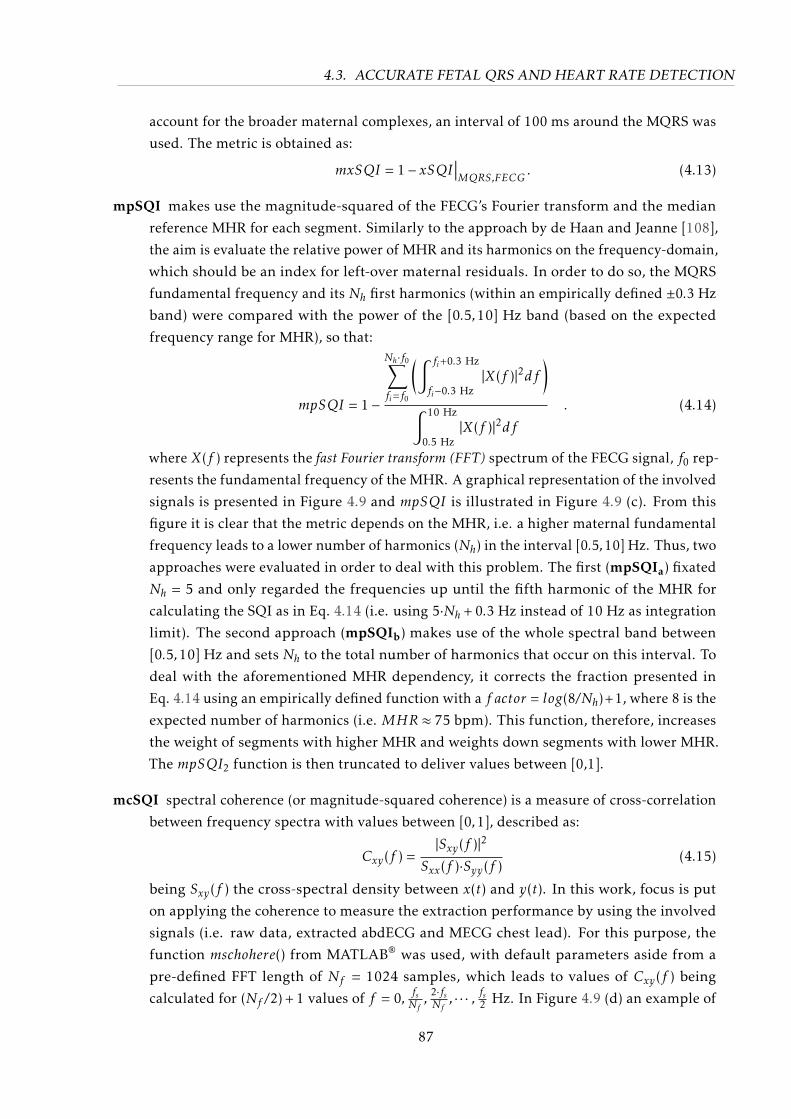
4.3. ACCURATE FETAL QRS AND HEART RATE DETECTION
account for the broader maternal complexes, an interval of 100 ms around the MQRS was
used. The metric is obtained as:
mxSQI = 1− xSQI∣∣∣MQRS,FECG
. (4.13)
mpSQI makes use the magnitude-squared of the FECG’s Fourier transform and the median
reference MHR for each segment. Similarly to the approach by de Haan and Jeanne [108],
the aim is evaluate the relative power of MHR and its harmonics on the frequency-domain,
which should be an index for left-over maternal residuals. In order to do so, the MQRS
fundamental frequency and its Nh first harmonics (within an empirically defined ±0.3 Hz
band) were compared with the power of the [0.5,10] Hz band (based on the expected
frequency range for MHR), so that:
mpSQI = 1−
Nh·f0∑fi=f0
(∫ fi+0.3 Hz
fi−0.3 Hz|X(f )|2df
)∫ 10 Hz
0.5 Hz|X(f )|2df
. (4.14)
where X(f ) represents the fast Fourier transform (FFT) spectrum of the FECG signal, f0 rep-
resents the fundamental frequency of the MHR. A graphical representation of the involved
signals is presented in Figure 4.9 and mpSQI is illustrated in Figure 4.9 (c). From this
figure it is clear that the metric depends on the MHR, i.e. a higher maternal fundamental
frequency leads to a lower number of harmonics (Nh) in the interval [0.5,10] Hz. Thus, two
approaches were evaluated in order to deal with this problem. The first (mpSQIa) fixated
Nh = 5 and only regarded the frequencies up until the fifth harmonic of the MHR for
calculating the SQI as in Eq. 4.14 (i.e. using 5·Nh + 0.3 Hz instead of 10 Hz as integration
limit). The second approach (mpSQIb) makes use of the whole spectral band between
[0.5,10] Hz and sets Nh to the total number of harmonics that occur on this interval. To
deal with the aforementioned MHR dependency, it corrects the fraction presented in
Eq. 4.14 using an empirically defined function with a f actor = log(8/Nh)+1, where 8 is the
expected number of harmonics (i.e. MHR ≈ 75 bpm). This function, therefore, increases
the weight of segments with higher MHR and weights down segments with lower MHR.
The mpSQI2 function is then truncated to deliver values between [0,1].
mcSQI spectral coherence (or magnitude-squared coherence) is a measure of cross-correlation
between frequency spectra with values between [0,1], described as:
Cxy(f ) =|Sxy(f )|2
Sxx(f )·Syy(f )(4.15)
being Sxy(f ) the cross-spectral density between x(t) and y(t). In this work, focus is put
on applying the coherence to measure the extraction performance by using the involved
signals (i.e. raw data, extracted abdECG and MECG chest lead). For this purpose, the
function mschohere() from MATLAB® was used, with default parameters aside from a
pre-defined FFT length of Nf = 1024 samples, which leads to values of Cxy(f ) being
calculated for (Nf /2) + 1 values of f = 0, fsNf ,2·fsNf, · · · , fs2 Hz. In Figure 4.9 (d) an example of
87

4.3. ACCURATE FETAL QRS AND HEART RATE DETECTION
successful and unsuccessful extraction are presented. Following this idea, two metrics
were developed, namely mcSQIa and mcSQIb. The first measures the similarity between
the MECG chest (i.e. x(t)) lead and extracted FECG (y(t)) on the [0,100] Hz band as:
mcSQIa = 1− 1Nf ′·∑f ′Cxy(f )df , (4.16)
with f ′⇐ f ≤ 100 Hz and Nf ′ being the number of frequencies in f that match the desired
band. The second metric, focuses on evaluating if the extraction method has included
artifacts on higher frequent spectrum of the extracted signal. This could occur, e.g. when
using the EKF algorithm Gaussian kernels do not perfectly fit a MQRS complex in a couple
samples, leaving behind some artifacts with high-frequency content (see Figure 4.9 (d) - on
the right). This was done by evaluating the coherence between the preprocessed abdECG
(x(t)) and extracted FECG (y(t)) on the band [60,100] Hz as follows:
mcSQIb =1Nf ′·∑f ′Cxy(f )df , for 60 Hz ≤ f ′ ≤ 100 Hz. (4.17)
miSQI metric based on the iSQI and on the premise that in cases where the FECG extraction
performs poorly, the MQRS residuals have larger amplitudes then the FQRSs themselves.
As a consequence, the sub-optimal extraction leads to MQRS peaks being detected (in-
stead of FQRS), which could be assessed by using the iSQI-like algorithm to compare
the detected extracted abdominal signal and MQRS reference. Therefore, the metric is
calculated using a 50 ms acceptance interval as:
miSQI = 1− iSQI∣∣∣MQRS,FQRS
. (4.18)
Since both detection-based SQIs and miSQI metrics (see Table 4.2) make use of FQRS de-
tectors, their outcomes are dependent on the FQRS detectors’ performance. In this work, five
publicly available FQRS detectors were evaluated as presented in Table 4.3. For further refer-
ence, the indices listed in this table are used to describe variants of SQI metrics to which they
are pertained, e.g. bSQI12 represents the bSQI evaluated using the maxsearch algorithm [363]
and jqrs [54] detectors.
88
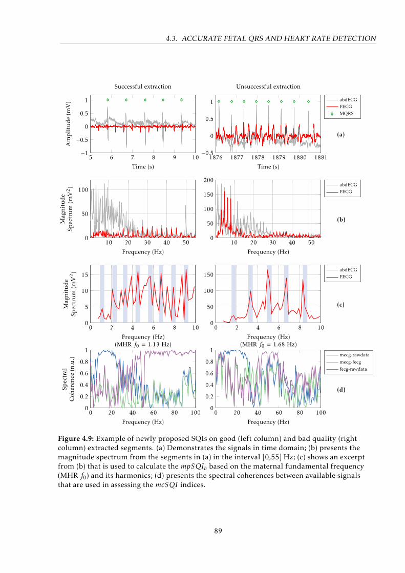
4.3. ACCURATE FETAL QRS AND HEART RATE DETECTION
5 6 7 8 9 10−1−0.5
0
0.5
1
Time (s)
Amplitude(m
V)
Successful extraction
1876 1877 1878 1879 1880 1881−0.5
0
0.5
1
Time (s)
Unsuccessful extraction
abdECGFECGMQRS
10 20 30 40 500
50
100
Frequency (Hz)
Mag
nitude
Spectrum
(mV2)
10 20 30 40 500
50
100
150
200
Frequency (Hz)
abdECGFECG
0 2 4 6 8 100
5
10
15
Frequency (Hz)(MHR f0 = 1.13 Hz)
Mag
nitude
Spectrum
(mV2)
0 2 4 6 8 100
50
100
150
Frequency (Hz)(MHR f0 = 1.68 Hz)
abdECGFECG
0 20 40 60 80 1000
0.2
0.4
0.6
0.8
1
Frequency (Hz)
Spectral
Coh
eren
ce(n.u.)
0 20 40 60 80 1000
0.2
0.4
0.6
0.8
1
Frequency (Hz)
mecg-rawdata
mecg-fecg
fecg-rawdata
(a)
(b)
(c)
(d)
Figure 4.9: Example of newly proposed SQIs on good (left column) and bad quality (rightcolumn) extracted segments. (a) Demonstrates the signals in time domain; (b) presents themagnitude spectrum from the segments in (a) in the interval [0,55] Hz; (c) shows an excerptfrom (b) that is used to calculate the mpSQIb based on the maternal fundamental frequency(MHR f0) and its harmonics; (d) presents the spectral coherences between available signalsthat are used in assessing the mcSQI indices.
89

4.3. ACCURATE FETAL QRS AND HEART RATE DETECTION
Tab
le4.
2:Su
mm
ary
offe
talS
QI
met
rics
use
din
this
wor
k.“C
at.”
refe
rsto
cate
gory
and
“Mu
lt.”
toth
em
eth
odre
quir
ing
mu
ltip
lech
an-
nels
orno
t(i
nclu
din
gM
EC
Gch
est
lead
).E
xcep
tfo
rth
eti
me
dom
ain
met
rics
,all
othe
rou
tpu
tbe
long
toR∈[
0,1]
.
Cat
.SQ
IM
ult
.D
escr
ipti
onR
ange
Ref
eren
ce
stdSQI
7st
and
ard
dev
iati
onof
sign
al,i
.e.stdSQI
=std
(x(t
))=
√ E[ (x(t
)−x(t)
)2]
R≥0
[89,
251]
(oth
erm
omen
t)
sSQI
7th
ird
mom
ent
(ske
wne
ss)o
fsi
gnal
,i.e
.sSQI
=E[(x
(t)−x(t)
)3]
std
(x(t
))3
R[8
9,25
1]
Time
kSQI
7fo
urt
hm
omen
t(k
urt
osis
)of
sign
al:kSQI
=E[(x
(t)−x(t)
)4]
std
(x(t
))4
R≥0
[89,
251]
pSQI
7re
lati
vep
ower
inth
eFQ
RS
com
ple
x:pSQI
=1−∫ 15H
z5Hz|X
(f)|2df /
∫ 45Hz
5Hz|X
(f)|2df,w
here
X(f
)=F(x(t)
)is
the
Fou
rier
tran
sfor
mofx(t)
.Diff
eren
tly
from
Lie
tal
.,th
ein
vers
eof
the
pow
erw
asap
pli
edto
rep
rese
ntM
QR
Ssu
pp
ress
ion.
[0,1
][8
9,25
1](i
nver
sed
)
Frequency
basSQI
7re
lati
vepo
wer
ofba
seli
ne(b
andw
idth
mod
ified
to[0,3
]Hz
toin
clud
em
ost
ofth
eE
HG
),i.e
.basSQI
=1∫ 3H
z0Hz|X
(f)|2df /
∫ 100 0Hz|X
(f)|2df
[0,1
][8
9,25
1](m
odifi
edba
nd)
bSQI
7p
erce
ntag
eof
beat
sco
mm
only
det
ecte
dby
two
diff
eren
tQ
RS
det
ecto
rs.T
his
met
ric
isno
thin
gm
ore
than
anac
cura
cym
easu
rebe
twee
nth
ose
det
ecto
rs(a
sd
escr
ibed
inSe
ctio
n3.
4.2)
.In
this
wor
kF
1m
etri
cis
use
d.
[0,1
][8
9,25
1]
iSQI
3p
erce
ntag
eof
beat
sd
etec
ted
oncu
rren
tle
adth
atw
ere
det
ecte
don
allo
ther
lead
s.[0,1
][8
9,25
1]
rSQI
7re
gula
rity
ofob
tain
edFQ
RS
inte
rval
srSQI
=1−N
out/Nd,w
hereNout
isth
enu
mbe
rof
outl
iers
(FHRV>
30bp
m)a
ndNd
the
tota
lnu
mbe
rof
det
ecti
ons
inth
ese
gmen
t[0,1
][5
4,21
1]
cSQI
7m
orp
holo
gyco
nfor
mit
ym
easu
refo
rFQ
RS
sim
ilar
ity
asp
rese
nted
inSe
ctio
n4.
3.1.
Neg
ativ
eco
rrel
atio
nsw
ere
set
toze
ro.
[0,1
]th
isw
ork,
base
don
[20]
Detection-based
xSQI
7ex
trav
agan
ceof
FQR
Sp
eaks
com
par
edto
its
surr
ound
ings
,exp
lain
edin
Sect
ion
4.3.
1(s
eeFi
g.4.
6).
[0,1
]th
isw
ork,
base
don
[20]
mxSQI
3an
alog
ous
to1−xSQI
cons
ider
ing
the
amp
litu
de
ofM
EC
Gco
mp
lexe
sre
sidu
als
(100
ms
win
dow
arou
ndM
QR
Sre
fere
nce
anno
tati
ons
of±5
0m
s)in
com
par
ison
wit
hsu
rrou
ndin
gex
trac
ted
abd
omin
alsi
gnal
s.[0,1
]th
isw
ork
mpSQI
3re
lati
vesp
ectr
alpo
wer
ofth
efi
rst
five
harm
onic
sof
the
MH
R(mpSQI a
)or
allh
arm
onic
sin
the
inte
rval
[0.5
,10]
Hz
(mpSQI b
).[0,1
]th
isw
ork,
base
don
[108
]
mcSQI
3sp
ectr
alco
here
nce
calc
ulat
edbe
twee
nav
aila
ble
sign
als.
Two
vari
ants
appl
ied:mcSQI a
uses
ME
CG
and
FEC
G(0
-100
Hz)
andmcSQI b
abd
EC
Gan
dFE
CG
(60-
100
Hz)
asp
revi
ousl
yex
pla
ined
.[0,1
]th
isw
ork,
base
don
[210
]
FECG-specific
miSQI
3si
mil
artoiSQI
betw
een
curr
ent
FQR
Sd
etec
tion
and
MQ
RS
refe
renc
e:miSQI
=1−iSQI M
QRS,FQRS
,aim
sat
exp
osin
gfa
lsel
yd
etec
ted
MQ
RS
resi
dual
s.[0,1
]th
isw
ork,
base
don
[152
]
90

4.3. ACCURATE FETAL QRS AND HEART RATE DETECTION
Table 4.3: Fetal QRS detectors evaluated in this work.
Index Name Description Reference
1maximalsearch
Simple algorithm that search for an absolute maximum within apre-defined window. [363]
2 jqrsImplementation of the Pan and Tompkins [320] peak energydetector. The algorithm is based on filtering, adaptivethresholding as well as forward and backward search.
[54, 320]
3P&T algo-rithm
Alternative implementation of the Pan-Tompkins algorithm. [320, 458]
4 gqrsQRS matched filter with a custom- built set of heuristics (such assearch back). It has been designed by George Moody, and is freelyavailable on Physionet
[161, 398]
5 wqrsDetector based on low-pass filtering, a nonlinear curve lengthtransformation and adaptive thresholding. [398, 480]
Classification using a Bayesian probabilistic classifier
With the aforementioned fetal SQIs at hand, one aim to evaluate if some combination of those
features can be indeed used in classifying good/bad quality FECG signals. This is performed by
using the annotated clinical data presented in Section 5.2.3 and visibility index from Table 5.6.
Several machine learning techniques are available to solve the classification problem at stake.
For the purpose of classification, a Naive Bayes classifier was employed using prior probability
and attribute probability densities given each class to model its posterior probability. During
classification, the class with the maximum posterior probability is usually selected [118]. How-
ever, in this work, the posterior probabilities were used to transform the classified values into
continuous valued outputs for further processing, as described in the following section [19].
In order to assess the expected classification performance of the trained Naive Bayes model,
i.e. the efficiency in assigning the signal quality based on the used SQIs to appropriate class,
a 10-fold cross validation was performed. Here, all 9,065 observations in the dataset (only
abdominal channels) were used to generate training and test sets, respectively. The final Naive
Bayes classification model was trained using all available observations as training set. To
avoid the trained classifier to be bounded by the training data’s class imbalance (as reported in
Section 5.2.3 and Fig. 4.10), the prior class probabilities were assumed to be equal for all classes
during performance assessment and when training the final classifier [19]. For completeness,
results are presented using both ordinal (Krippendorf’s αK ) and nominal (Cohen’s κ) agreement
measures, presented in Section 5.2.3.
Kalman filter approach to multichannel consensus
As described by Oster and Clifford [315], several methods have been proposed for fusing
multichannel HR estimates using SQI-like metrics. Amongst those are simplistic weighted
averages and computationally demanding machine learning approaches. This consensus, there
are generally two types of possible combinations, namely channel selection or fusion. In channel
91
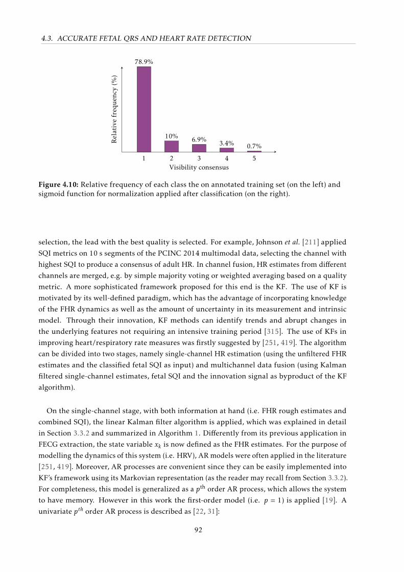
4.3. ACCURATE FETAL QRS AND HEART RATE DETECTION
1 2 3 4 5
78.9%
10% 6.9% 3.4% 0.7%
Visibility consensus
Relativefreq
uen
cy(%
)
Figure 4.10: Relative frequency of each class the on annotated training set (on the left) andsigmoid function for normalization applied after classification (on the right).
selection, the lead with the best quality is selected. For example, Johnson et al. [211] applied
SQI metrics on 10 s segments of the PCINC 2014 multimodal data, selecting the channel with
highest SQI to produce a consensus of adult HR. In channel fusion, HR estimates from different
channels are merged, e.g. by simple majority voting or weighted averaging based on a quality
metric. A more sophisticated framework proposed for this end is the KF. The use of KF is
motivated by its well-defined paradigm, which has the advantage of incorporating knowledge
of the FHR dynamics as well as the amount of uncertainty in its measurement and intrinsic
model. Through their innovation, KF methods can identify trends and abrupt changes in
the underlying features not requiring an intensive training period [315]. The use of KFs in
improving heart/respiratory rate measures was firstly suggested by [251, 419]. The algorithm
can be divided into two stages, namely single-channel HR estimation (using the unfiltered FHR
estimates and the classified fetal SQI as input) and multichannel data fusion (using Kalman
filtered single-channel estimates, fetal SQI and the innovation signal as byproduct of the KF
algorithm).
On the single-channel stage, with both information at hand (i.e. FHR rough estimates and
combined SQI), the linear Kalman filter algorithm is applied, which was explained in detail
in Section 3.3.2 and summarized in Algorithm 1. Differently from its previous application in
FECG extraction, the state variable xk is now defined as the FHR estimates. For the purpose of
modelling the dynamics of this system (i.e. HRV), AR models were often applied in the literature
[251, 419]. Moreover, AR processes are convenient since they can be easily implemented into
KF’s framework using its Markovian representation (as the reader may recall from Section 3.3.2).
For completeness, this model is generalized as a pth order AR process, which allows the system
to have memory. However in this work the first-order model (i.e. p = 1) is applied [19]. A
univariate pth order AR process is described as [22, 31]:
92
4.3. ACCURATE FETAL QRS AND HEART RATE DETECTION
ak+1 =∑pi=1
(ϕi,k · ak−i+1 +wk
),
ak+1 = ϕTk· ak +wk ,
(4.19)
where i ∈ [1,p] is the index, xk denotes the order, ϕi,k are the time-dependent AR coefficients
and wk is an additive zero-mean white Gaussian noise process. By applying this modelling
into a KF framework, one aims to obtain a linear regression of the p previous FHR measures
(FHRk−1 · · ·FHRk−p) to estimate the current FHRk , represented in Eq. 4.20:
FHR(n) = [FHR(n− 1) ·ϕ1 +FHR(n− 2) ·ϕ2 + ...+FHR(n− p) ·ϕp] (4.20)
Equations 4.19-4.20 can be modelled into KF’s space-state representation as Eqs. 3.1 and
3.2. The state variable xk ∈ Rp×1 is defined as the signal of interest (i.e. the FHR p previous
estimates), the state vector yk∈ Rq×1 contains the observations (rough FHR values), wk is the
process noise and vk the observational noise. The filter noise covariance matrices are defined by
w ∼N (0,Qk) and v ∼N (0,Rk). The state transition matrix A is the p × p matrix, describing the
expected dynamics of our state (see Eq. 4.21), while the observational matrix H is a 1× q null
vector, except for its first element which is unitary.
xk =[FHRk ,FHRk−1, · · · ,FHRk−p+1
]T
and F =
ϕ1 ϕ2 . . . ϕp−1 ϕp1 0 . . . 0 0
0 1 . . . 0 0...
. . ....
0 0 . . . 1 0
(4.21)
he KF’s gain is mostly influenced by its defined process and observational noise covariance
matrices (Qk and Rk). In order to integrate the information on the signal quality, Li et al. [251]
proposed modulating the KF’s measurement covariance matrix as described in Eq. 4.22.
Rk ≡ R0 · exp(1/SQI2k − 1) (4.22)
where SQIk (with SQI ∈ [0,1]) denotes the time dependent combined signal quality and R0 is
the initial value of measurement covariance matrix, which is signal dependent. The employed
nonlinear weighting function leads to Rk → R0 (if SQIk → 1) and Rk →∞ (if SQIk → 0). The
adaptive covariance matrix enhances the influence of cleaner estimates on the filter’s outcome,
providing the filter with a more rapid response to sudden changes in the signal quality [315].
n this work, to obtain continuous SQI values, the use of posterior probabilities P (i,k) from the
previously depicted classifier is proposed. Thus, the continuous valued SQI output is generated
by SQIk =∑i=A,B,...,E P (i,k)∗vi,k . The initial values for the measurement and process covariance
matrices, were empirically determined using a grid-search algorithm (as in [22]) on the first
minute of each annotated dataset, for avoiding over-training. The calibration procedure resulted
93
4.4. CHAPTER SUMMARY
on R0 = 10−3 and Q0 = 1.
After obtaining a Kalman filtered FHR estimate for each available channel, the second stage
(i.e. sensor data fusion) step takes place. This multichannel consensus is obtained by using both
KF innovation (νk) and consensus SQI signal such that:
x′k =Nc∑s
∏Nci=1,i,s σ
2k,i∑Nc
i=1
(∏Ncj=1,j,i σ
2k,j
) · xk,s (4.23)
where x′k represents the final FHR estimate, xk,s is the current FHR estimate for each available
channel s at time-step k and σ2k,s ≡
(νk,s/SQIk,s
)2. This approach was likewise proposed by [251].
The accuracy of our estimated FHR was evaluated based on two measures, as described
in Section 3.5.2, namely the HDR and RMSE. In order to generate the FHR reference, FQRS
complexes were manually annotated as described in Section 5.2.4. The reference FHR was then
obtained by calculating the mean of the annotated RR intervals in windows of 5 seconds with
1-second overlap.
Applicability to other biosignals
As a side note, in a preliminary work [22] this author made use of a similar strategy for
obtaining more accurate HR estimates from camera-based photoplethysmogram (cbPPG) record-
ings by means of SQI measures for video images. cbPPG is a contactless measuring technique,
which based on the slight variations of skin color during a heart cycle, allows the acquisition of
cardio-respiratory signals using conventional cameras [194]. As usually occurs, the ease with
which it is recorded is counterbalanced by subject’s movements and light changes that generally
lead to a signal of interest with low SNR. At the IBMT several works have been performed on
this topic [243, 459, 460, 478]. In order to cope with the low SNR of the cbPPG signal, the green
channel is often preferred. Next, one or more region of interest (ROI)s are usually selected from
the output of a face detection algorithm. The resulting cbPPG signal is obtained by averaging
the intensity signal within these ROIs. Notwithstanding, even after some bandpass filtering, the
pulsatile signal obtained is often buried into noise.
In Andreotti et al. [22], 10 s segments were processed using the Short Time Fast FourierTransform (STFT), whose main frequency was assumed to represent the HR. The KF approach,
presented in the previous section, was then used for improving HR detection. For this purpose,
two SQI metrics were applied, namely frequency-based (mpSQIa, as previously described
in this section) and a novel image velocity-based (vSQI) index. This latter measure aims at
detecting motion artefacts, which usually influences the reliability of the cbPPG measurement
and respective HR estimate.
4.4 Chapter Summary
In this chapter, several improvements in NIFECG extraction, detection and heart rate estima-
tion were proposed. In Section 4.2, two major improvements in the EKF2/EKF24 models were
94

4.4. CHAPTER SUMMARY
proposed, namely the time-varying covariance matrices (vEKF2/vEKF24) and the unknown
input addition to its model (i.e. uiEKF2), to better represent the non-Gaussian nature of fetal
peaks. In Section 4.3, methods to improve the detection of FQRS complexes (i.e. location
accuracy for individual peaks) or their time-average (i.e. FHR) were proposed. Both those
methods had in common the necessity of metrics to improve their specificity. For this reason,
several novel fetal SQI metrics were suggested (see Section 4.3.2). Fetal QRS locations was
improved with the eQRS method, which exhaustively attempts to optimize a global objective
function based on each individual peak’s SQI values. Fetal HR estimation was improved using a
KF approach, whose noise covariance matrix Rk was adapted using a Naive Bayes classifier and
several novel SQI metrics. In the next chapter, the data material produced during this work is
presented.
95


In God we trust, all others (must) bring data
– controversially attributed to W. Edwards Deming
5Data Material
Data is a crucial part of training and testing of signal processing algorithms. In the previous
chapters, novel methods for NIFECG were proposed, however due to the lack of publicly
available NIFECG databases, as mentioned in Section 3.2.4, the clinical usage of NIFECG has
been hindered. Therefore, in this work alternative sources of data were sought. For this
purpose, a simulator and large database of simulated data was created in cooperation with
the Institute of Biomedical Engineering at the University of Oxford, which is presented in
Section 5.1. Concomitantly, to validate the performance of signal processing algorithms in a
real-world scenario, clinical recordings were performed at the University Hospital of Leipzig
(see Section 5.2).
5.1 Simulated Data
Simulated data provides means for training NIFECG processing algorithms with gold-
standard information on the accurate location of FQRS, MQRS and FECG signal waveform. In
the following sections, the toolbox and simulated database developed during this work are
described.
5.1.1 The FECG Synthetic Generator (FECGSYN)
A straightforward manner of representing the myocardial electrical activity is to use a three-
dimensional time-varying vector, whose origin is modelled as a punctual source at the center
of the heart. This heart dipole vector can be written as d(t) = v1(t)i + v2(t)j + v3(t)k, where i, j,
k are unit vectors for the three-dimensional body axes and vn(t) with n ∈ [1,3] depicts three
orthogonal signals, which constitute the VCG, and are used to represent the heart cycle. The
potential difference φ(r, t)−φ0(r, t) measured at a point on the torso (i.e. volume conductor)
97
5.1. SIMULATED DATA
and a reference potential (negative electrode, as explained in Section 3.2.3) is represented in
Equation 5.1 [49, 50]:
φ(r, t)−φ0(r0, t) =d(t)
4πε0
(r(t)|r(t)|3 −
r0(t)|r0(t)|3
), (5.1)
where r(t) is the vector from the dipole center to observational point, ε0 is the permittivity of the
volume conductor (here regarded as isotropic1 and unitary). As the heart dipole d(t) changes
with time (i.e. during a heart cycle, i.e. time-point on the VCG waveform) or its position r(t)
(e.g. with respiration), the potential difference is expected to vary [50].
Based on this simplified representation of the cardiac electrical activity by McSharry et al.[275] and Sameni et al. [364] proposed a model for generating realistic ECG waveforms. The
model is built on the premise that a set of Nk Gaussian kernel functions can be used to approxi-
mate VCG cycles. By modelling all three dimensions of VCG signals (see Fig. 5.1), available for
example at Physionet’s PTB Diagnostic ECG Database2 [68, 161], one can attain a 3-D model
for the heart’s electrical activity. Adopting the simplified polar coordinate system (rather than
Cartesian) as proposed by Sameni [362], the model can be described as:
dp(t) =
Nk∑n=1
δαpnλ(bpn
)2∆θpn,k−1exp
−∆(θpn,k−1)2
2(bpn)2
for p ∈ i , j , k , (5.2)
where each component dp(t) of the dipole d(t) is represented by a sum of Nk Gaussian kernels.
The variable ∆θn,k = θk −φn denotes the phase of the nth Gaussian at time step k, φn being
the position of the each kernel inside the template. Parameters αn, bn and φn correspond to
the amplitude, width, and position of the nth Gaussian kernel, respectively (see Fig. 5.1). The
angular frequency (λ) and sampling period (δ) determine the time progression (or pace) of
the signal. In McSharry et al. [275], realistic HRV changes are introduced by making λ time
variant, designed to well-represent the respiratory sinus arrhythmia and the response to Mayer
waves [213]. Furthermore, a projection matrix built upon the cardiac dipole model was used
to project the VCG waveforms onto the observational points (i.e. electrode positions) on the
surface of the volume conductor, thus obtaining propagated ECG signals. The projection matrix
contains information about the permittivity of the conductor (assumed constant), dipole origin
and relative location between observing electrodes and source. Figure 5.2 shows exemplary
fetal and maternal punctual cardiac sources within a cylindric volume conductor. From this
Figure, the positive electrodes (numbered from 1-34) and the ground electrode can be seen.
The negative potential (φ0(t)) is calculated as the mean of all available electrodes’ signals. The
original implementation of McSharry et al. [275]’s adult ECG simulation model is available on
Physionet3.
Following the works from McSharry et al. [275], Sameni et al. [364] suggested the use of this
1 According to [468], for frequencies below 1000 Hz, the capacitive component of tissue impedance, the inductiveand the electromagnetic propagation effect in biological tissues can be neglected.
2 Available at Physionet under https://www.physionet.org/physiobank/database/ptbdb/3 ECGSYN toolbox, available at https://www.physionet.org/physiotools/ecgsyn/
98
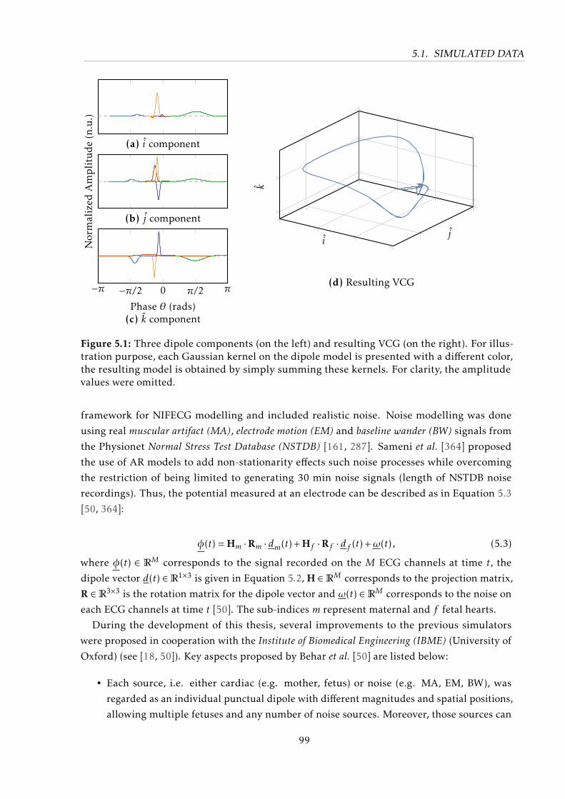
5.1. SIMULATED DATA
Normalized
Amplitude(n.u.)
−π −π/2 0 π/2 π
Phase θ (rads)
(a) i component
(b) j component
(c) k component
ij
k
(d) Resulting VCG
Figure 5.1: Three dipole components (on the left) and resulting VCG (on the right). For illus-tration purpose, each Gaussian kernel on the dipole model is presented with a different color,the resulting model is obtained by simply summing these kernels. For clarity, the amplitudevalues were omitted.
framework for NIFECG modelling and included realistic noise. Noise modelling was done
using real muscular artifact (MA), electrode motion (EM) and baseline wander (BW) signals from
the Physionet Normal Stress Test Database (NSTDB) [161, 287]. Sameni et al. [364] proposed
the use of AR models to add non-stationarity effects such noise processes while overcoming
the restriction of being limited to generating 30 min noise signals (length of NSTDB noise
recordings). Thus, the potential measured at an electrode can be described as in Equation 5.3
[50, 364]:
φ(t) = Hm ·Rm · dm(t) + Hf ·Rf · df (t) +ω(t) , (5.3)
where φ(t) ∈ RM corresponds to the signal recorded on the M ECG channels at time t, the
dipole vector d(t) ∈R1×3 is given in Equation 5.2, H ∈RM corresponds to the projection matrix,
R ∈R3×3 is the rotation matrix for the dipole vector and ω(t) ∈RM corresponds to the noise on
each ECG channels at time t [50]. The sub-indices m represent maternal and f fetal hearts.
During the development of this thesis, several improvements to the previous simulators
were proposed in cooperation with the Institute of Biomedical Engineering (IBME) (University of
Oxford) (see [18, 50]). Key aspects proposed by Behar et al. [50] are listed below:
• Each source, i.e. either cardiac (e.g. mother, fetus) or noise (e.g. MA, EM, BW), was
regarded as an individual punctual dipole with different magnitudes and spatial positions,
allowing multiple fetuses and any number of noise sources. Moreover, those sources can
99
5.1. SIMULATED DATA
be spatially distributed freely within the volume conductor;
• Translatory and rotatory motion of dipole sources were implemented by designing H(t)
and R(t) to be time variant. This improvement allows the modelling of fetal/maternal
respiratory movements and fetal/noise movements inside the volume conductor;
• Different SNRs were assigned to each source, meaning each fetus/noise could have distinct
strengths;
• Both HR signal and SNR strength can be modulated, for example, using a hyperbolic
tangent function to increase/decrease HR or noises SNR;
• VCG models for ectopic beats derived from the PTB Diagnostic ECG Database4 [68, 161]
were included.
These improvements to the model and encapsulated design enable the production of maternal
and fetal signals in both physiological and pathological scenarios as well as a number of
non-stationary phenomena. The enhanced simulator, named Fetal ECG Synthetic Generator(FECGSYN), was released5 under an open-source GNU General Public License (GPL) license.
Its main purpose is to facilitate stress-testing of NIFECG algorithms under varied conditions.
Further, FECGSYN was used to generate a large simulated dataset and benchmark routine
described in the following section.
5.1.2 The FECG Synthetic Database (FECGSYNDB)
In this work, the FECGSYNDB was developed and made publicly available on Physionet6
[18, 161]. The FECGSYNDB is a large database of simulated signals, which enables reproducible
research in adult and NIFECG areas. Similarly to the FECGSYN toolbox, the FECGSYNDB was
created in partnership with the IBME from the University of Oxford.
The simulated data was generated using the FECGSYN [50] (Section 5.1.1). The modeled
volume conductor is presented in Figure 5.2. As observational points, 34 simulated channels
(32 abdominal and 2 MECG chest channels) were included (see Fig. 5.2). The ground electrode
was positioned on the back of the cylinder at the polar coordinates π,0.5,−0.3. The electrode
configuration was designed to span across most of the simulated “maternal abdomen”. A total of
seven physiological events (i.e. described in table 5.1) was considered. For each case, the heart
dipole models (for mother and fetuses) were generated ten times by randomly selecting one of
the nine VCGs available in the FECGSYN toolbox. Five different levels of additive noise were
included (0,3,6,9, and 12 dB). Simulations were repeated five times, re-generating noise signals
on every iteration, to obtain a more representative database. Overall a total of 7×10×5×5 = 1750
synthetic signals were produced. Each simulation consisted of 5 minutes abdominal mixtures
projected onto , totalizing 145.8 hours of multichannel data and 1.1 million fetal peaks. Several
4 Available at Physionet: https://www.physionet.org/physiobank/database/ptbdb/5 Available at: http://www.fecgsyn.com6 Available at Physionet: https://physionet.org/physiobank/database/fecgsyndb/
100
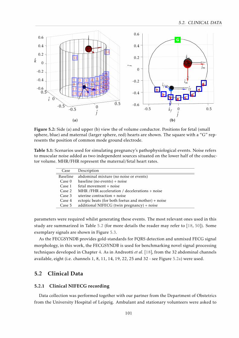
5.2. CLINICAL DATA
-0.5
0
0.5
i
-0.5 00.5
j
k
0.6
0.4
0.2
0
-0.2
-0.4
-0.6
(a)
jf
kf
if
jm
km
im
j-0.5 0 0.5
0.6
0.4
0.2
0
-0.2
-0.4
-0.6
i
(b)
Figure 5.2: Side (a) and upper (b) view the of volume conductor. Positions for fetal (smallsphere, blue) and maternal (larger sphere, red) hearts are shown. The square with a “G” rep-resents the position of common mode ground electrode.
Table 5.1: Scenarios used for simulating pregnancy’s pathophysiological events. Noise refersto muscular noise added as two independent sources situated on the lower half of the conduc-tor volume. MHR/FHR represent the maternal/fetal heart rates.
Case Description
Baseline abdominal mixture (no noise or events)Case 0 baseline (no events) + noiseCase 1 fetal movement + noiseCase 2 MHR /FHR acceleration / decelerations + noiseCase 3 uterine contraction + noiseCase 4 ectopic beats (for both foetus and mother) + noiseCase 5 additional NIFECG (twin pregnancy) + noise
parameters were required whilst generating these events. The most relevant ones used in this
study are summarized in Table 5.2 (for more details the reader may refer to [18, 50]). Some
exemplary signals are shown in Figure 5.3.
As the FECGSYNDB provides gold-standards for FQRS detection and unmixed FECG signal
morphology, in this work, the FECGSYNDB is used for benchmarking novel signal processing
techniques developed in Chapter 4. As in Andreotti et al. [18], from the 32 abdominal channels
available, eight (i.e. channels 1, 8, 11, 14, 19, 22, 25 and 32 - see Figure 5.2a) were used.
5.2 Clinical Data
5.2.1 Clinical NIFECG recording
Data collection was performed together with our partner from the Department of Obstetrics
from the University Hospital of Leipzig. Ambulant and stationary volunteers were asked to
101
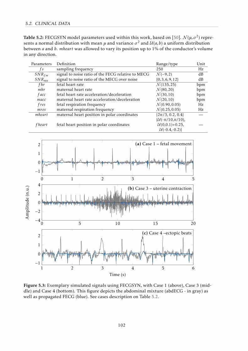
5.2. CLINICAL DATA
Table 5.2: FECGSYN model parameters used within this work, based on [50]. N (µ,σ2) repre-sents a normal distribution with mean µ and variance σ2 and U (a,b) a uniform distributionbetween a and b. mheart was allowed to vary its position up to 1% of the conductor’s volumein any direction.
Parameters Definition Range/type Unitf s sampling frequency 250 Hz
SNRf m signal to noise ratio of the FECG relative to MECG N (−9,2) dBSNRmn signal to noise ratio of the MECG over noise 0,3,6,9,12 dBf hr fetal heart rate N (135,25) bpmmhr maternal heart rate N (80,20) bpmf acc fetal heart rate acceleration/deceleration N (30,10) bpmmacc maternal heart rate acceleration/deceleration N (20,10) bpmf res fetal respiration frequency N (0.90,0.05) Hzmres maternal respiration frequency N (0.25,0.05) Hzmheart maternal heart position in polar coordinates 2π/3, 0.2, 0.4 —
f heart fetal heart position in polar coordinatesU (-π/10,π/10),U (0,0.1)+0.25,U (-0.4,-0.2)
—
0 1 2 3 4 5
−10
1
2
0 5 10 15 20−4−20
2
4
Amplitude(n.u.)
1 2 3 4 5 6−10
1
2
Time (s)
(a) Case 1 – fetal movement
(b) Case 3 – uterine contraction
(c) Case 4 –ectopic beats
Figure 5.3: Exemplary simulated signals using FECGSYN, with Case 1 (above), Case 3 (mid-dle) and Case 4 (bottom). This figure depicts the abdominal mixture (abdECG - in gray) aswell as propagated FECG (blue). See cases description on Table 5.2.
102
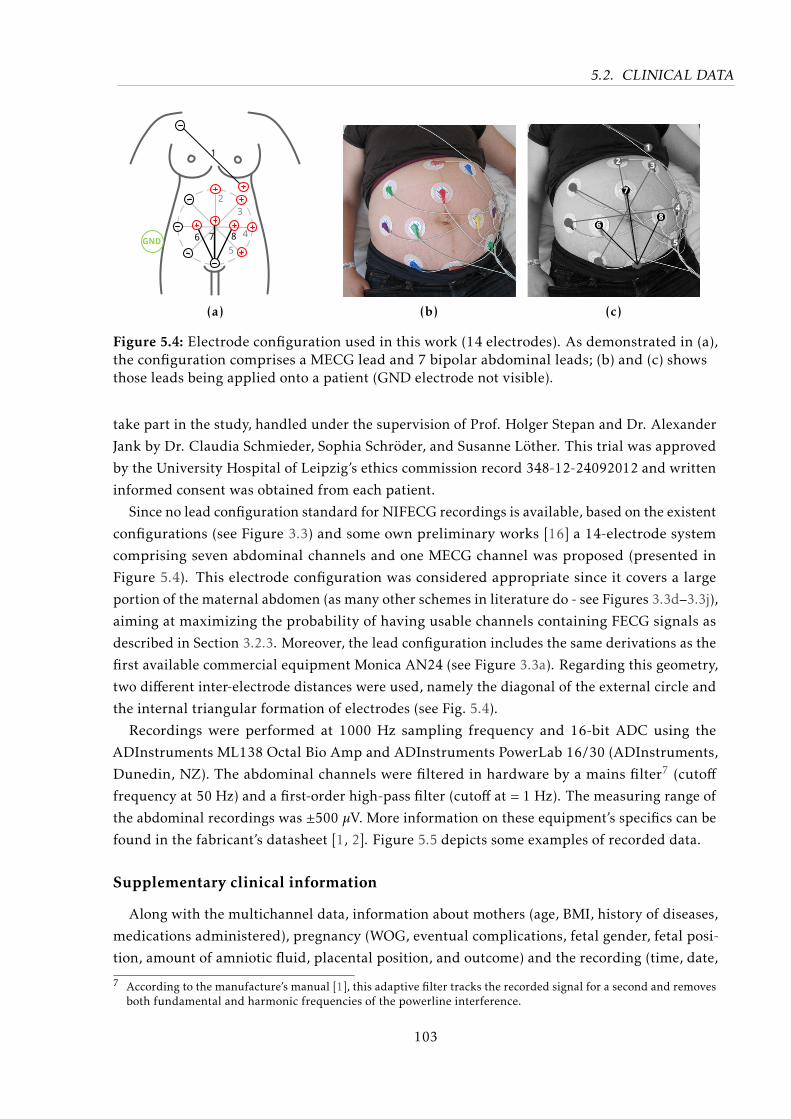
5.2. CLINICAL DATA
1
4
3
2
5
86 7GND
(a) (b)
2 3
4
5
6
7
8
1
(c)
Figure 5.4: Electrode configuration used in this work (14 electrodes). As demonstrated in (a),the configuration comprises a MECG lead and 7 bipolar abdominal leads; (b) and (c) showsthose leads being applied onto a patient (GND electrode not visible).
take part in the study, handled under the supervision of Prof. Holger Stepan and Dr. Alexander
Jank by Dr. Claudia Schmieder, Sophia Schröder, and Susanne Löther. This trial was approved
by the University Hospital of Leipzig’s ethics commission record 348-12-24092012 and written
informed consent was obtained from each patient.
Since no lead configuration standard for NIFECG recordings is available, based on the existent
configurations (see Figure 3.3) and some own preliminary works [16] a 14-electrode system
comprising seven abdominal channels and one MECG channel was proposed (presented in
Figure 5.4). This electrode configuration was considered appropriate since it covers a large
portion of the maternal abdomen (as many other schemes in literature do - see Figures 3.3d–3.3j),
aiming at maximizing the probability of having usable channels containing FECG signals as
described in Section 3.2.3. Moreover, the lead configuration includes the same derivations as the
first available commercial equipment Monica AN24 (see Figure 3.3a). Regarding this geometry,
two different inter-electrode distances were used, namely the diagonal of the external circle and
the internal triangular formation of electrodes (see Fig. 5.4).
Recordings were performed at 1000 Hz sampling frequency and 16-bit ADC using the
ADInstruments ML138 Octal Bio Amp and ADInstruments PowerLab 16/30 (ADInstruments,
Dunedin, NZ). The abdominal channels were filtered in hardware by a mains filter7 (cutofffrequency at 50 Hz) and a first-order high-pass filter (cutoff at = 1 Hz). The measuring range of
the abdominal recordings was ±500 µV. More information on these equipment’s specifics can be
found in the fabricant’s datasheet [1, 2]. Figure 5.5 depicts some examples of recorded data.
Supplementary clinical information
Along with the multichannel data, information about mothers (age, BMI, history of diseases,
medications administered), pregnancy (WOG, eventual complications, fetal gender, fetal posi-
tion, amount of amniotic fluid, placental position, and outcome) and the recording (time, date,
7 According to the manufacture’s manual [1], this adaptive filter tracks the recorded signal for a second and removesboth fundamental and harmonic frequencies of the powerline interference.
103
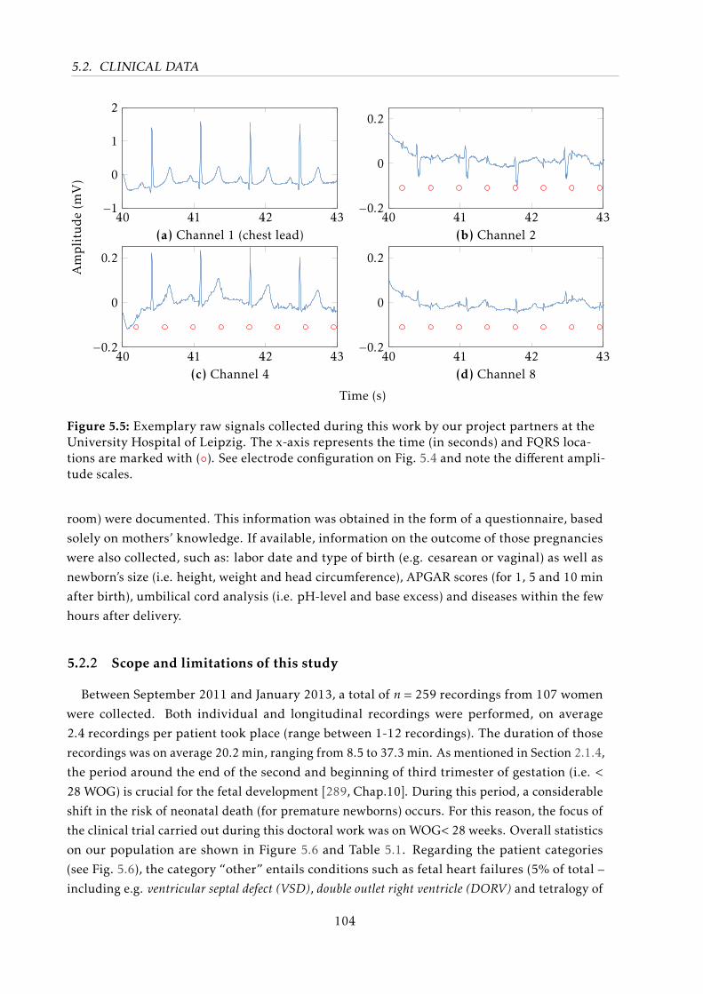
5.2. CLINICAL DATA
40 41 42 43−1
0
1
2
40 41 42 43−0.2
0
0.2
40 41 42 43−0.2
0
0.2
40 41 42 43−0.2
0
0.2
(a) Channel 1 (chest lead) (b) Channel 2
(c) Channel 4 (d) Channel 8
Amplitude(m
V)
Time (s)
Figure 5.5: Exemplary raw signals collected during this work by our project partners at theUniversity Hospital of Leipzig. The x-axis represents the time (in seconds) and FQRS loca-tions are marked with (). See electrode configuration on Fig. 5.4 and note the different ampli-tude scales.
room) were documented. This information was obtained in the form of a questionnaire, based
solely on mothers’ knowledge. If available, information on the outcome of those pregnancies
were also collected, such as: labor date and type of birth (e.g. cesarean or vaginal) as well as
newborn’s size (i.e. height, weight and head circumference), APGAR scores (for 1, 5 and 10 min
after birth), umbilical cord analysis (i.e. pH-level and base excess) and diseases within the few
hours after delivery.
5.2.2 Scope and limitations of this study
Between September 2011 and January 2013, a total of n = 259 recordings from 107 women
were collected. Both individual and longitudinal recordings were performed, on average
2.4 recordings per patient took place (range between 1-12 recordings). The duration of those
recordings was on average 20.2 min, ranging from 8.5 to 37.3 min. As mentioned in Section 2.1.4,
the period around the end of the second and beginning of third trimester of gestation (i.e. <
28 WOG) is crucial for the fetal development [289, Chap.10]. During this period, a considerable
shift in the risk of neonatal death (for premature newborns) occurs. For this reason, the focus of
the clinical trial carried out during this doctoral work was on WOG< 28 weeks. Overall statistics
on our population are shown in Figure 5.6 and Table 5.1. Regarding the patient categories
(see Fig. 5.6), the category “other” entails conditions such as fetal heart failures (5% of total –
including e.g. ventricular septal defect (VSD), double outlet right ventricle (DORV) and tetralogy of
104
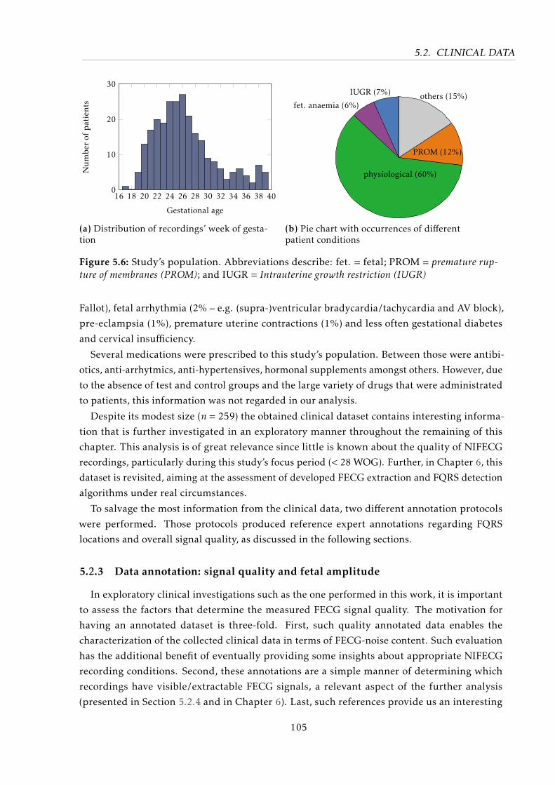
5.2. CLINICAL DATA
16 18 20 22 24 26 28 30 32 34 36 38 400
10
20
30
Gestational age
Numbe
rof
patients
(a) Distribution of recordings’ week of gesta-tion
IUGR (7%)
fet. anaemia (6%)
physiological (60%)
PROM (12%)
others (15%)
(b) Pie chart with occurrences of differentpatient conditions
Figure 5.6: Study’s population. Abbreviations describe: fet. = fetal; PROM = premature rup-ture of membranes (PROM); and IUGR = Intrauterine growth restriction (IUGR)
Fallot), fetal arrhythmia (2% – e.g. (supra-)ventricular bradycardia/tachycardia and AV block),
pre-eclampsia (1%), premature uterine contractions (1%) and less often gestational diabetes
and cervical insufficiency.
Several medications were prescribed to this study’s population. Between those were antibi-
otics, anti-arrhytmics, anti-hypertensives, hormonal supplements amongst others. However, due
to the absence of test and control groups and the large variety of drugs that were administrated
to patients, this information was not regarded in our analysis.
Despite its modest size (n = 259) the obtained clinical dataset contains interesting informa-
tion that is further investigated in an exploratory manner throughout the remaining of this
chapter. This analysis is of great relevance since little is known about the quality of NIFECG
recordings, particularly during this study’s focus period (< 28 WOG). Further, in Chapter 6, this
dataset is revisited, aiming at the assessment of developed FECG extraction and FQRS detection
algorithms under real circumstances.
To salvage the most information from the clinical data, two different annotation protocols
were performed. Those protocols produced reference expert annotations regarding FQRS
locations and overall signal quality, as discussed in the following sections.
5.2.3 Data annotation: signal quality and fetal amplitude
In exploratory clinical investigations such as the one performed in this work, it is important
to assess the factors that determine the measured FECG signal quality. The motivation for
having an annotated dataset is three-fold. First, such quality annotated data enables the
characterization of the collected clinical data in terms of FECG-noise content. Such evaluation
has the additional benefit of eventually providing some insights about appropriate NIFECG
recording conditions. Second, these annotations are a simple manner of determining which
recordings have visible/extractable FECG signals, a relevant aspect of the further analysis
(presented in Section 5.2.4 and in Chapter 6). Last, such references provide us an interesting
105
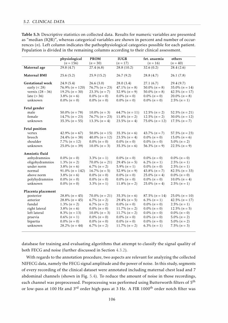
5.2. CLINICAL DATA
Table 5.3: Descriptive statistics on collected data. Results for numeric variables are presentedas “median (IQR)”, whereas categorical variables are shown in percent and number of occur-rences (n). Left column indicates the pathophysiological categories possible for each patient.Population is divided in the remaining columns according to their clinical assessment.
physiological(n = 156)
PROM(n = 30)
IUGR(n = 17)
fet. anaemia(n = 16)
others(n = 40)
Maternal age 29.8 (4.7) 27.4 (6.8) 28.8 (10.2) 32.6 (0.2) 28.4 (2.6)
Maternal BMI 25.6 (5.2) 25.9 (15.2) 26.7 (9.2) 28.8 (4.7) 26.1 (7.8)
Gestational week 24.9 (5.4) 26.6 (3.0) 28.0 (3.4) 27.1 (6.7) 29.4 (9.7)early (< 28) 76.9% (n = 120) 76.7% (n = 23) 47.1% (n = 8) 50.0% (n = 8) 35.0% (n = 14)vernix (28− 36) 19.2% (n = 30) 23.3% (n = 7) 52.9% (n = 9) 50.0% (n = 8) 42.5% (n = 17)late (> 36) 3.8% (n = 6) 0.0% (n = 0) 0.0% (n = 0) 0.0% (n = 0) 20.0% (n = 8)unknown 0.0% (n = 0) 0.0% (n = 0) 0.0% (n = 0) 0.0% (n = 0) 2.5% (n = 1)
Fetal gendermale 50.0% (n = 78) 10.0% (n = 3) 64.7% (n = 11) 12.5% (n = 2) 52.5% (n = 21)female 14.7% (n = 23) 76.7% (n = 23) 11.8% (n = 2) 12.5% (n = 2) 30.0% (n = 12)unknown 35.3% (n = 55) 13.3% (n = 4) 23.5% (n = 4) 75.0% (n = 12) 17.5% (n = 7)
Fetal positionvertex 42.9% (n = 67) 50.0% (n = 15) 35.3% (n = 6) 43.7% (n = 7) 57.5% (n = 23)breech 24.4% (n = 38) 40.0% (n = 12) 23.5% (n = 4) 0.0% (n = 0) 15.0% (n = 6)shoulder 7.7% (n = 12) 0.0% (n = 0) 0.0% (n = 0) 0.0% (n = 0) 5.0% (n = 2)unknown 25.0% (n = 39) 10.0% (n = 3) 35.3% (n = 6) 56.3% (n = 9) 22.5% (n = 9)
Amniotic fluidanhydramnios 0.0% (n = 0) 3.3% (n = 1) 0.0% (n = 0) 0.0% (n = 0) 0.0% (n = 0)oligohydramnios 1.3% (n = 2) 70.0% (n = 21) 29.4% (n = 5) 6.2% (n = 1) 2.5% (n = 1)under norm 3.8% (n = 6) 6.7% (n = 2) 5.9% (n = 1) 0.0% (n = 0) 2.5% (n = 1)normal 91.0% (n = 142) 16.7% (n = 5) 52.9% (n = 9) 43.8% (n = 7) 82.5% (n = 33)above norm 3.8% (n = 6) 0.0% (n = 0) 0.0% (n = 0) 25.0% (n = 4) 0.0% (n = 0)polyhydramnios 0.0% (n = 0) 0.0% (n = 0) 0.0% (n = 0) 0.0% (n = 0) 10.0% (n = 4)unknown 0.0% (n = 0) 3.3% (n = 1) 11.8% (n = 2) 25.0% (n = 4) 2.5% (n = 1)
Placenta placementposterior 28.8% (n = 45) 70.0% (n = 21) 35.3% (n = 6) 87.5% (n = 14) 25.0% (n = 10)anterior 28.8% (n = 45) 6.7% (n = 2) 29.4% (n = 5) 6.3% (n = 1) 42.5% (n = 17)fundal 1.3% (n = 2) 6.7% (n = 2) 0.0% (n = 0) 0.0% (n = 0) 2.5% (n = 1)right lateral 3.8% (n = 6) 0.0% (n = 0) 11.7% (n = 2) 0.0% (n = 0) 12.5% (n = 5)left lateral 8.3% (n = 13) 10.0% (n = 3) 11.7% (n = 2) 0.0% (n = 0) 0.0% (n = 0)praevia 0.6% (n = 1) 0.0% (n = 0) 0.0% (n = 0) 0.0% (n = 0) 5.0% (n = 2)bipartia 0.0% (n = 0) 0.0% (n = 0) 0.0% (n = 0) 0.0% (n = 0) 5.0% (n = 2)unknown 28.2% (n = 44) 6.7% (n = 2) 11.7% (n = 2) 6.3% (n = 1) 7.5% (n = 3)
database for training and evaluating algorithms that attempt to classify the signal quality of
both FECG and noise (further discussed in Section 4.3.2).
With regards to the annotation procedure, two aspects are relevant for analyzing the collected
NIFECG data, namely the FECG signal amplitude and the power of noise. In this study, segments
of every recording of the clinical dataset were annotated including maternal chest lead and 7
abdominal channels (shown in Fig. 5.4). To reduce the amount of noise in those recordings,
each channel was preprocessed. Preprocessing was performed using Butterworth filters of 5th
or low-pass at 100 Hz and 3rd order high-pass at 3 Hz. A FIR 1000th order notch filter was
106
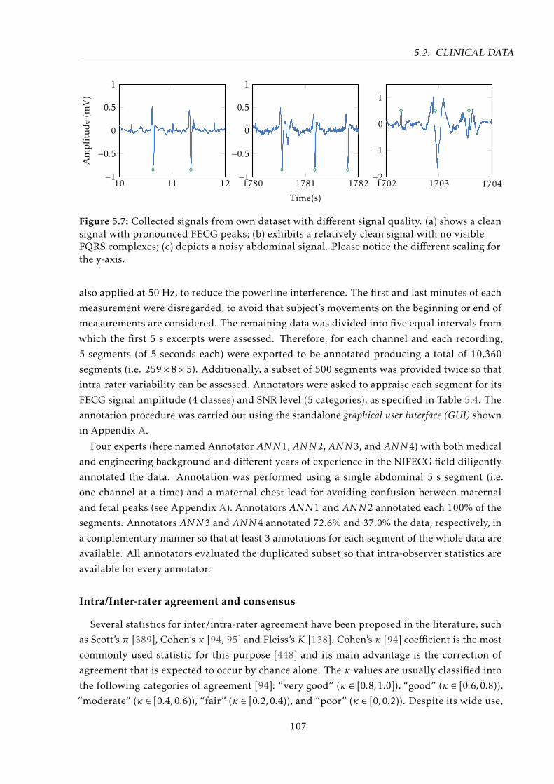
5.2. CLINICAL DATA
10 11 12−1
−0.5
0
0.5
1Amplitude(m
V)
1780 1781 1782−1
−0.5
0
0.5
1
Time(s)
1702 1703 1704−2
−1
0
1
Figure 5.7: Collected signals from own dataset with different signal quality. (a) shows a cleansignal with pronounced FECG peaks; (b) exhibits a relatively clean signal with no visibleFQRS complexes; (c) depicts a noisy abdominal signal. Please notice the different scaling forthe y-axis.
also applied at 50 Hz, to reduce the powerline interference. The first and last minutes of each
measurement were disregarded, to avoid that subject’s movements on the beginning or end of
measurements are considered. The remaining data was divided into five equal intervals from
which the first 5 s excerpts were assessed. Therefore, for each channel and each recording,
5 segments (of 5 seconds each) were exported to be annotated producing a total of 10,360
segments (i.e. 259×8×5). Additionally, a subset of 500 segments was provided twice so that
intra-rater variability can be assessed. Annotators were asked to appraise each segment for its
FECG signal amplitude (4 classes) and SNR level (5 categories), as specified in Table 5.4. The
annotation procedure was carried out using the standalone graphical user interface (GUI) shown
in Appendix A.
Four experts (here named Annotator ANN1, ANN2, ANN3, and ANN4) with both medical
and engineering background and different years of experience in the NIFECG field diligently
annotated the data. Annotation was performed using a single abdominal 5 s segment (i.e.
one channel at a time) and a maternal chest lead for avoiding confusion between maternal
and fetal peaks (see Appendix A). Annotators ANN1 and ANN2 annotated each 100% of the
segments. Annotators ANN3 and ANN4 annotated 72.6% and 37.0% the data, respectively, in
a complementary manner so that at least 3 annotations for each segment of the whole data are
available. All annotators evaluated the duplicated subset so that intra-observer statistics are
available for every annotator.
Intra/Inter-rater agreement and consensus
Several statistics for inter/intra-rater agreement have been proposed in the literature, such
as Scott’s π [389], Cohen’s κ [94, 95] and Fleiss’s K [138]. Cohen’s κ [94] coefficient is the most
commonly used statistic for this purpose [448] and its main advantage is the correction of
agreement that is expected to occur by chance alone. The κ values are usually classified into
the following categories of agreement [94]: “very good” (κ ∈ [0.8,1.0]), “good” (κ ∈ [0.6,0.8)),
“moderate” (κ ∈ [0.4,0.6)), “fair” (κ ∈ [0.2,0.4)), and “poor” (κ ∈ [0,0.2)). Despite its wide use,
107
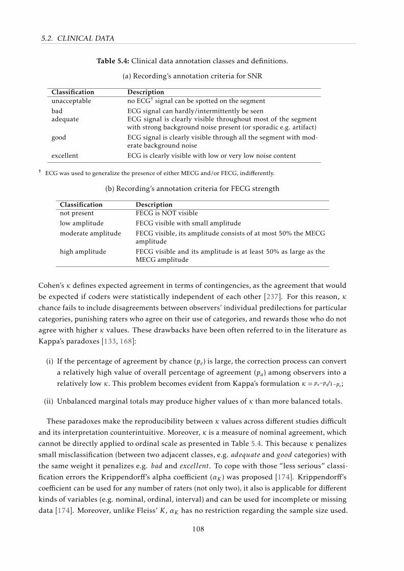
5.2. CLINICAL DATA
Table 5.4: Clinical data annotation classes and definitions.
(a) Recording’s annotation criteria for SNR
Classification Descriptionunacceptable no ECG† signal can be spotted on the segment
bad ECG signal can hardly/intermittently be seenadequate ECG signal is clearly visible throughout most of the segment
with strong background noise present (or sporadic e.g. artifact)
good ECG signal is clearly visible through all the segment with mod-erate background noise
excellent ECG is clearly visible with low or very low noise content
† ECG was used to generalize the presence of either MECG and/or FECG, indifferently.
(b) Recording’s annotation criteria for FECG strength
Classification Descriptionnot present FECG is NOT visible
low amplitude FECG visible with small amplitude
moderate amplitude FECG visible, its amplitude consists of at most 50% the MECGamplitude
high amplitude FECG visible and its amplitude is at least 50% as large as theMECG amplitude
Cohen’s κ defines expected agreement in terms of contingencies, as the agreement that would
be expected if coders were statistically independent of each other [237]. For this reason, κ
chance fails to include disagreements between observers’ individual predilections for particular
categories, punishing raters who agree on their use of categories, and rewards those who do not
agree with higher κ values. These drawbacks have been often referred to in the literature as
Kappa’s paradoxes [133, 168]:
(i) If the percentage of agreement by chance (pe) is large, the correction process can convert
a relatively high value of overall percentage of agreement (pa) among observers into a
relatively low κ. This problem becomes evident from Kappa’s formulation κ = pa−pe/1−pe;
(ii) Unbalanced marginal totals may produce higher values of κ than more balanced totals.
These paradoxes make the reproducibility between κ values across different studies difficult
and its interpretation counterintuitive. Moreover, κ is a measure of nominal agreement, which
cannot be directly applied to ordinal scale as presented in Table 5.4. This because κ penalizes
small misclassification (between two adjacent classes, e.g. adequate and good categories) with
the same weight it penalizes e.g. bad and excellent. To cope with those “less serious” classi-
fication errors the Krippendorff’s alpha coefficient (αK ) was proposed [174]. Krippendorff’s
coefficient can be used for any number of raters (not only two), it also is applicable for different
kinds of variables (e.g. nominal, ordinal, interval) and can be used for incomplete or missing
data [174]. Moreover, unlike Fleiss’ K , αK has no restriction regarding the sample size used.
108
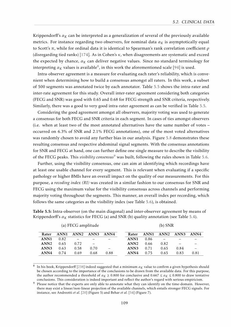
5.2. CLINICAL DATA
Krippendorff’s αK can be interpreted as a generalization of several of the previously available
metrics. For instance regarding two observers, for nominal data αK is asymptotically equal
to Scott’s π, while for ordinal data it is identical to Spearman’s rank correlation coefficient ρ
(disregarding tied ranks) [174]. As in Cohen’s κ, when disagreements are systematic and exceed
the expected by chance, αK can deliver negative values. Since no standard terminology for
interpreting αK values is available8, in this work the aforementioned scale [94] is used.
Intra-observer agreement is a measure for evaluating each rater’s reliability, which is conve-
nient when determining how to build a consensus amongst all raters. In this work, a subset
of 500 segments was annotated twice by each annotator. Table 5.5 shows the intra-rater and
inter-rate agreement for this study. Overall inter-rater agreement considering both categories
(FECG and SNR) was good with 0.65 and 0.68 for FECG strength and SNR criteria, respectively.
Similarly, there was a good to very good intra-rater agreement as can be verified in Table 5.5.
Considering the good agreement amongst all observers, majority voting was used to generate
a consensus for both FECG and SNR criteria in each segment. In cases of ties amongst observers
(i.e. when at least two of the most annotated alternatives have the same number of votes –
occurred on 6.3% of SNR and 2.1% FECG annotations), one of the most voted alternatives
was randomly chosen to avoid any further bias in our analysis. Figure 5.8 demonstrates these
resulting consensus and respective abdominal signal segments. With the consensus annotations
for SNR and FECG at hand, one can further define one single measure to describe the visibility
of the FECG peaks. This visibility consensus9 was built, following the rules shown in Table 5.6.
Further, using the visibility consensus, one can aim at identifying which recordings have
at least one usable channel for every segment. This is relevant when evaluating if a specific
pathology or higher BMIs have an overall impact on the quality of our measurements. For this
purpose, a recoding index (RI) was created in a similar fashion to our consensus for SNR and
FECG using the maximum value for the visibility consensus across channels and performing
majority voting throughout the segments. This manner, an overall index per recording, which
follows the same categories as the visibility index (see Table 5.6), is obtained.
Table 5.5: Intra-observer (on the main diagonal) and inter-observer agreement by means ofKrippendorff’s αK statistics for FECG (a) and SNR (b) quality annotation (see Table 5.4).
(a) FECG amplitude
Rater ANN1 ANN2 ANN3 ANN4ANN1 0.82 – – –ANN2 0.65 0.72 –ANN3 0.63 0.58 0.70 –ANN4 0.74 0.69 0.68 0.88
(b) SNR
Rater ANN1 ANN2 ANN3 ANN4ANN1 0.86 – – –ANN2 0.66 0.82 – –ANN3 0.71 0.65 0.84 –ANN4 0.75 0.65 0.83 0.81
8 In his book, Krippendorff [238] indeed suggested that a minimum αK value to confirm a given hypothesis shouldbe chosen according to the importance of the conclusions to be drawn from the available data. For this purpose,the author recommended a threshold of αK ≥ 0.800 for conclusive and 0.667 ≤ αK ≤ 0.800 to draw tentativeconclusions. This consideration is indeed important and reflect the author’s regard with serious empiricism.
9 Please notice that the experts are only able to annotate what they can identify on the time-domain. However,there may exist a linear/non-linear projection of the available channels, which entails stronger FECG signals. Forinstance, see Andreotti et al. [20] (Figure 5) and Behar et al. [54] (Figure 7).
109
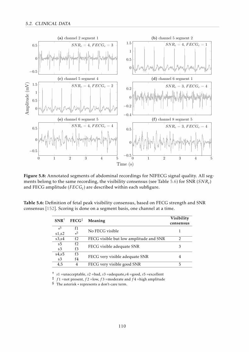
5.2. CLINICAL DATA
−0.5
0
0.5 SNRc = 4, FECGc = 3
(a) channel 2 segment 1
0
0.5
1
1.5 SNRc = 4, FECGc = 1
(b) channel 5 segment 2
0
0.5
1
1.5 SNRc = 4, FECGc = 2
Am
plit
ude
(mV
)
(c) channel 5 segment 4
−0.4
−0.2
0
0.2SNRc = 3, FECGc = 4
(d) channel 6 segment 1
0 1 2 3 4 5
−0.5
0
0.5SNRc = 4, FECGc = 4
Time (s)
(e) channel 6 segment 5
0 1 2 3 4 5−0.5
0
0.5SNRc = 3, FECGc = 4
(f) channel 8 segment 5
Figure 5.8: Annotated segments of abdominal recordings for NIFECG signal quality. All seg-ments belong to the same recording, the visibility consensus (see Table 5.6) for SNR (SNRc)and FECG amplitude (FECGc) are described within each subfigure.
Table 5.6: Definition of fetal peak visibility consensus, based on FECG strength and SNRconsensus [152]. Scoring is done on a segment basis, one channel at a time.
SNR† FECG‡ MeaningVisibilityconsensus
∗§s1,s2
f1∗§ No FECG visible 1
s3,s4 f2 FECG visible but low amplitude and SNR 2s5s3
f2f3 FECG visible adequate SNR 3
s4,s5s3
f3f4 FECG very visible adequate SNR 4
4,5 4 FECG very visible good SNR 5
† s1 =unacceptable, s2 =bad, s3 =adequate,s4 =good, s5 =excellent‡ f 1 =not present, f 2 =low, f 3 =moderate and f 4 =high amplitude§ The asterisk ∗ represents a don’t-care term.
110
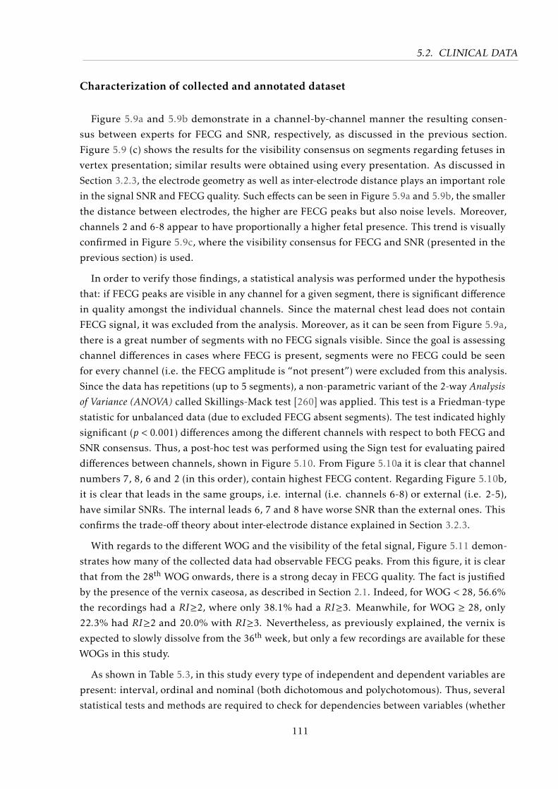
5.2. CLINICAL DATA
Characterization of collected and annotated dataset
Figure 5.9a and 5.9b demonstrate in a channel-by-channel manner the resulting consen-
sus between experts for FECG and SNR, respectively, as discussed in the previous section.
Figure 5.9 (c) shows the results for the visibility consensus on segments regarding fetuses in
vertex presentation; similar results were obtained using every presentation. As discussed in
Section 3.2.3, the electrode geometry as well as inter-electrode distance plays an important role
in the signal SNR and FECG quality. Such effects can be seen in Figure 5.9a and 5.9b, the smaller
the distance between electrodes, the higher are FECG peaks but also noise levels. Moreover,
channels 2 and 6-8 appear to have proportionally a higher fetal presence. This trend is visually
confirmed in Figure 5.9c, where the visibility consensus for FECG and SNR (presented in the
previous section) is used.
In order to verify those findings, a statistical analysis was performed under the hypothesis
that: if FECG peaks are visible in any channel for a given segment, there is significant difference
in quality amongst the individual channels. Since the maternal chest lead does not contain
FECG signal, it was excluded from the analysis. Moreover, as it can be seen from Figure 5.9a,
there is a great number of segments with no FECG signals visible. Since the goal is assessing
channel differences in cases where FECG is present, segments were no FECG could be seen
for every channel (i.e. the FECG amplitude is “not present”) were excluded from this analysis.
Since the data has repetitions (up to 5 segments), a non-parametric variant of the 2-way Analysisof Variance (ANOVA) called Skillings-Mack test [260] was applied. This test is a Friedman-type
statistic for unbalanced data (due to excluded FECG absent segments). The test indicated highly
significant (p < 0.001) differences among the different channels with respect to both FECG and
SNR consensus. Thus, a post-hoc test was performed using the Sign test for evaluating paired
differences between channels, shown in Figure 5.10. From Figure 5.10a it is clear that channel
numbers 7, 8, 6 and 2 (in this order), contain highest FECG content. Regarding Figure 5.10b,
it is clear that leads in the same groups, i.e. internal (i.e. channels 6-8) or external (i.e. 2-5),
have similar SNRs. The internal leads 6, 7 and 8 have worse SNR than the external ones. This
confirms the trade-off theory about inter-electrode distance explained in Section 3.2.3.
With regards to the different WOG and the visibility of the fetal signal, Figure 5.11 demon-
strates how many of the collected data had observable FECG peaks. From this figure, it is clear
that from the 28th WOG onwards, there is a strong decay in FECG quality. The fact is justified
by the presence of the vernix caseosa, as described in Section 2.1. Indeed, for WOG < 28, 56.6%
the recordings had a RI≥2, where only 38.1% had a RI≥3. Meanwhile, for WOG ≥ 28, only
22.3% had RI≥2 and 20.0% with RI≥3. Nevertheless, as previously explained, the vernix is
expected to slowly dissolve from the 36th week, but only a few recordings are available for these
WOGs in this study.
As shown in Table 5.3, in this study every type of independent and dependent variables are
present: interval, ordinal and nominal (both dichotomous and polychotomous). Thus, several
statistical tests and methods are required to check for dependencies between variables (whether
111
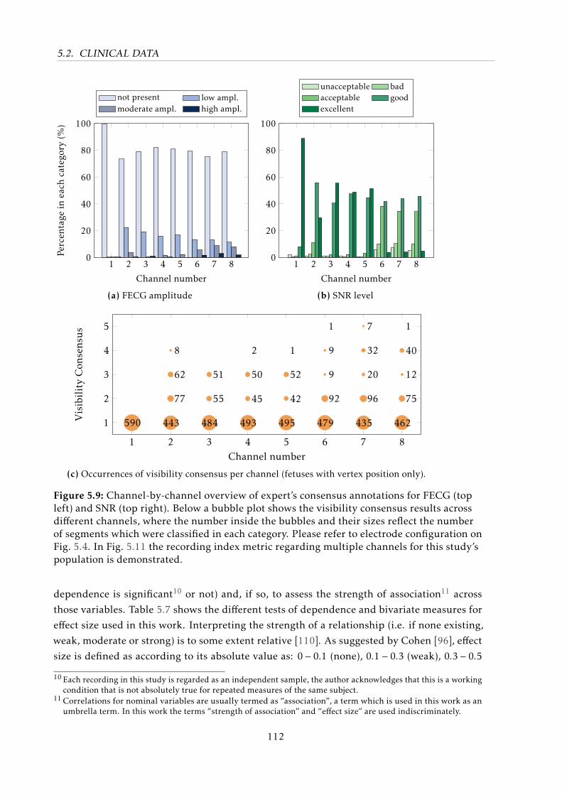
5.2. CLINICAL DATA
1 2 3 4 5 6 7 80
20
40
60
80
100
Channel number
Percen
tage
ineach
catego
ry(%
)
not present low ampl.moderate ampl. high ampl.
(a) FECG amplitude
1 2 3 4 5 6 7 80
20
40
60
80
100
Channel number
unacceptable badacceptable goodexcellent
(b) SNR level
1 2 3 4 5 6 7 8
1
2
3
4
5
Channel number
VisibilityCon
sens
us
590 443
77
62
8
484
55
51
493
45
50
2
495
42
52
1
479
92
9
9
1
435
96
20
32
7
462
75
12
40
1
(c) Occurrences of visibility consensus per channel (fetuses with vertex position only).
Figure 5.9: Channel-by-channel overview of expert’s consensus annotations for FECG (topleft) and SNR (top right). Below a bubble plot shows the visibility consensus results acrossdifferent channels, where the number inside the bubbles and their sizes reflect the numberof segments which were classified in each category. Please refer to electrode configuration onFig. 5.4. In Fig. 5.11 the recording index metric regarding multiple channels for this study’spopulation is demonstrated.
dependence is significant10 or not) and, if so, to assess the strength of association11 across
those variables. Table 5.7 shows the different tests of dependence and bivariate measures for
effect size used in this work. Interpreting the strength of a relationship (i.e. if none existing,
weak, moderate or strong) is to some extent relative [110]. As suggested by Cohen [96], effect
size is defined as according to its absolute value as: 0 − 0.1 (none), 0.1 − 0.3 (weak), 0.3 − 0.5
10 Each recording in this study is regarded as an independent sample, the author acknowledges that this is a workingcondition that is not absolutely true for repeated measures of the same subject.
11 Correlations for nominal variables are usually termed as “association”, a term which is used in this work as anumbrella term. In this work the terms “strength of association” and “effect size” are used indiscriminately.
112
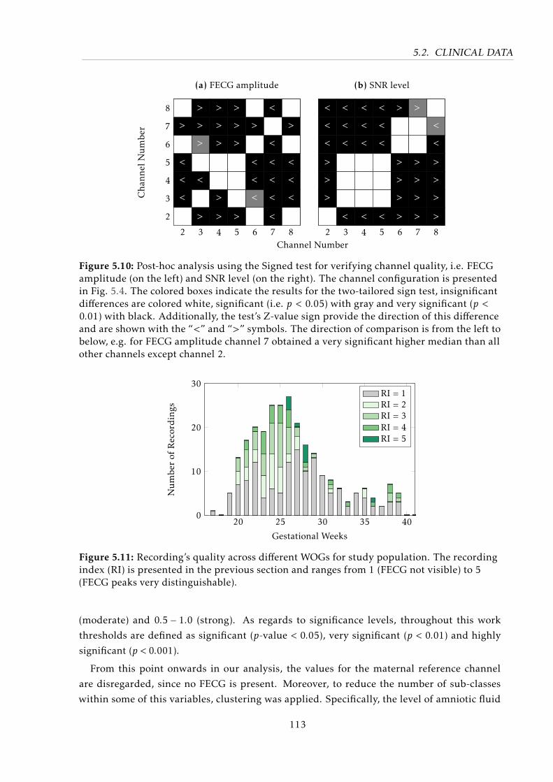
5.2. CLINICAL DATA
2 3 4 5 6 7 8
2
3
4
5
6
7
8 :)
>
:)
<
<
<
:)
>
>
>
:)
<
:)
>
>
>
>
:)
:)
>
>
>
>
>
:)
:)
:)
>
:)
>
:)
<
<
<
:)
<
:)
<
<
<
<
<
:)
>
:)
<
<
<
:)
Channel Number
Cha
nnel
Numbe
r
(a) FECG amplitude
2 3 4 5 6 7 8
<
<
<
>
>
>
:)
<
<
<
:)
:)
:)
<
<
<
<
:)
:)
:)
<
<
<
<
:)
:)
:)
<
>
:)
:)
>
>
>
>
>
:)
:)
>
>
>
>
:)
<
<
>
>
>
>
(b) SNR level
Figure 5.10: Post-hoc analysis using the Signed test for verifying channel quality, i.e. FECGamplitude (on the left) and SNR level (on the right). The channel configuration is presentedin Fig. 5.4. The colored boxes indicate the results for the two-tailored sign test, insignificantdifferences are colored white, significant (i.e. p < 0.05) with gray and very significant (p <0.01) with black. Additionally, the test’s Z-value sign provide the direction of this differenceand are shown with the “<” and “>” symbols. The direction of comparison is from the left tobelow, e.g. for FECG amplitude channel 7 obtained a very significant higher median than allother channels except channel 2.
20 25 30 35 400
10
20
30
Gestational Weeks
Numbe
rof
Recordings
RI = 1RI = 2RI = 3RI = 4RI = 5
Figure 5.11: Recording’s quality across different WOGs for study population. The recordingindex (RI) is presented in the previous section and ranges from 1 (FECG not visible) to 5(FECG peaks very distinguishable).
(moderate) and 0.5 − 1.0 (strong). As regards to significance levels, throughout this work
thresholds are defined as significant (p-value < 0.05), very significant (p < 0.01) and highly
significant (p < 0.001).
From this point onwards in our analysis, the values for the maternal reference channel
are disregarded, since no FECG is present. Moreover, to reduce the number of sub-classes
within some of this variables, clustering was applied. Specifically, the level of amniotic fluid
113
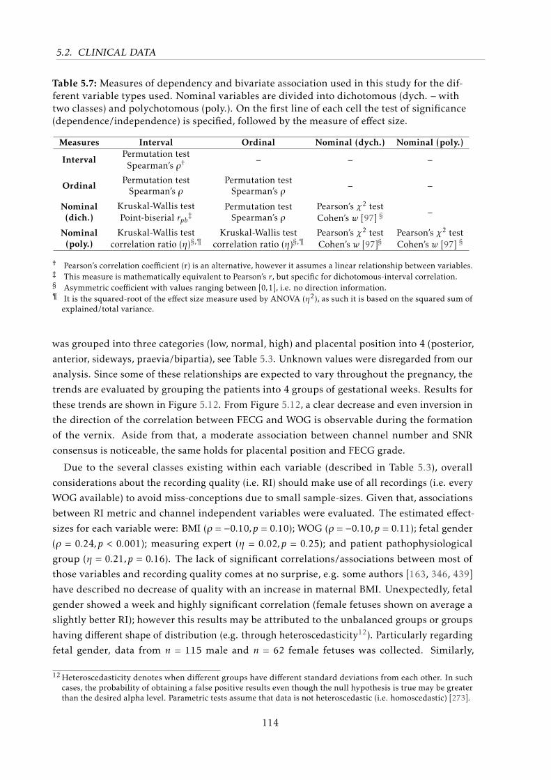
5.2. CLINICAL DATA
Table 5.7: Measures of dependency and bivariate association used in this study for the dif-ferent variable types used. Nominal variables are divided into dichotomous (dych. – withtwo classes) and polychotomous (poly.). On the first line of each cell the test of significance(dependence/independence) is specified, followed by the measure of effect size.
Measures Interval Ordinal Nominal (dych.) Nominal (poly.)
IntervalPermutation test
Spearman’s ρ† – – –
OrdinalPermutation test
Spearman’s ρPermutation test
Spearman’s ρ – –
Nominal(dich.)
Kruskal-Wallis testPoint-biserial rpb‡
Permutation testSpearman’s ρ
Pearson’s χ2 testCohen’s w [97] § –
Nominal(poly.)
Kruskal-Wallis testcorrelation ratio (η)§,¶
Kruskal-Wallis testcorrelation ratio (η)§,¶
Pearson’s χ2 testCohen’s w [97]§
Pearson’s χ2 testCohen’s w [97] §
† Pearson’s correlation coefficient (r) is an alternative, however it assumes a linear relationship between variables.‡ This measure is mathematically equivalent to Pearson’s r, but specific for dichotomous-interval correlation.§ Asymmetric coefficient with values ranging between [0,1], i.e. no direction information.¶ It is the squared-root of the effect size measure used by ANOVA (η2), as such it is based on the squared sum of
explained/total variance.
was grouped into three categories (low, normal, high) and placental position into 4 (posterior,
anterior, sideways, praevia/bipartia), see Table 5.3. Unknown values were disregarded from our
analysis. Since some of these relationships are expected to vary throughout the pregnancy, the
trends are evaluated by grouping the patients into 4 groups of gestational weeks. Results for
these trends are shown in Figure 5.12. From Figure 5.12, a clear decrease and even inversion in
the direction of the correlation between FECG and WOG is observable during the formation
of the vernix. Aside from that, a moderate association between channel number and SNR
consensus is noticeable, the same holds for placental position and FECG grade.
Due to the several classes existing within each variable (described in Table 5.3), overall
considerations about the recording quality (i.e. RI) should make use of all recordings (i.e. every
WOG available) to avoid miss-conceptions due to small sample-sizes. Given that, associations
between RI metric and channel independent variables were evaluated. The estimated effect-
sizes for each variable were: BMI (ρ = −0.10,p = 0.10); WOG (ρ = −0.10,p = 0.11); fetal gender
(ρ = 0.24,p < 0.001); measuring expert (η = 0.02,p = 0.25); and patient pathophysiological
group (η = 0.21,p = 0.16). The lack of significant correlations/associations between most of
those variables and recording quality comes at no surprise, e.g. some authors [163, 346, 439]
have described no decrease of quality with an increase in maternal BMI. Unexpectedly, fetal
gender showed a week and highly significant correlation (female fetuses shown on average a
slightly better RI); however this results may be attributed to the unbalanced groups or groups
having different shape of distribution (e.g. through heteroscedasticity12). Particularly regarding
fetal gender, data from n = 115 male and n = 62 female fetuses was collected. Similarly,
12 Heteroscedasticity denotes when different groups have different standard deviations from each other. In suchcases, the probability of obtaining a false positive results even though the null hypothesis is true may be greaterthan the desired alpha level. Parametric tests assume that data is not heteroscedastic (i.e. homoscedastic) [273].
114
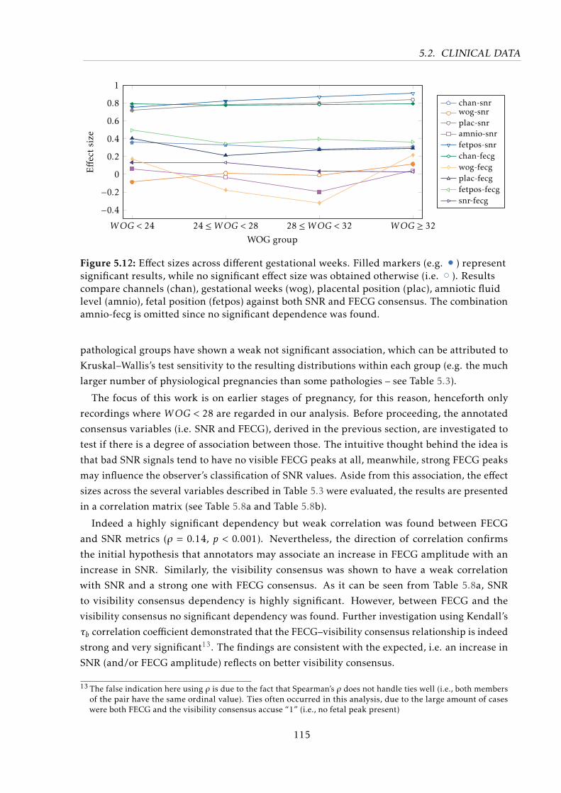
5.2. CLINICAL DATA
WOG < 24 24 ≤WOG < 28 28 ≤WOG < 32 WOG ≥ 32
−0.4−0.2
0
0.2
0.4
0.6
0.8
1
WOG group
Effe
ctsize
chan-snrwog-snrplac-snramnio-snrfetpos-snrchan-fecgwog-fecgplac-fecgfetpos-fecgsnr-fecg
Figure 5.12: Effect sizes across different gestational weeks. Filled markers (e.g. ) representsignificant results, while no significant effect size was obtained otherwise (i.e. ). Resultscompare channels (chan), gestational weeks (wog), placental position (plac), amniotic fluidlevel (amnio), fetal position (fetpos) against both SNR and FECG consensus. The combinationamnio-fecg is omitted since no significant dependence was found.
pathological groups have shown a weak not significant association, which can be attributed to
Kruskal–Wallis’s test sensitivity to the resulting distributions within each group (e.g. the much
larger number of physiological pregnancies than some pathologies – see Table 5.3).
The focus of this work is on earlier stages of pregnancy, for this reason, henceforth only
recordings where WOG < 28 are regarded in our analysis. Before proceeding, the annotated
consensus variables (i.e. SNR and FECG), derived in the previous section, are investigated to
test if there is a degree of association between those. The intuitive thought behind the idea is
that bad SNR signals tend to have no visible FECG peaks at all, meanwhile, strong FECG peaks
may influence the observer’s classification of SNR values. Aside from this association, the effect
sizes across the several variables described in Table 5.3 were evaluated, the results are presented
in a correlation matrix (see Table 5.8a and Table 5.8b).
Indeed a highly significant dependency but weak correlation was found between FECG
and SNR metrics (ρ = 0.14, p < 0.001). Nevertheless, the direction of correlation confirms
the initial hypothesis that annotators may associate an increase in FECG amplitude with an
increase in SNR. Similarly, the visibility consensus was shown to have a weak correlation
with SNR and a strong one with FECG consensus. As it can be seen from Table 5.8a, SNR
to visibility consensus dependency is highly significant. However, between FECG and the
visibility consensus no significant dependency was found. Further investigation using Kendall’s
τb correlation coefficient demonstrated that the FECG–visibility consensus relationship is indeed
strong and very significant13. The findings are consistent with the expected, i.e. an increase in
SNR (and/or FECG amplitude) reflects on better visibility consensus.
13 The false indication here using ρ is due to the fact that Spearman’s ρ does not handle ties well (i.e., both membersof the pair have the same ordinal value). Ties often occurred in this analysis, due to the large amount of caseswere both FECG and the visibility consensus accuse “1” (i.e., no fetal peak present)
115
5.2. CLINICAL DATA
Aside from the assessment metrics, some other effects can be observed in Table 5.8. Some
of these effects, such as the reduction of amniotic fluid levels with an increase in WOG, can be
physiologically explained. Meanwhile, the cause of other effects such as the association between
fetal and placental position are less evident. From Table 5.8 (b) it is noticeable that a strong
and significant association was found between channel number and FECG/visibility consensus,
which confirms the previous results. Strong associations between placental position and SNR
level (η = 0.76, p < 0.01) and moderate association for placental position – FECG (η = 0.30,
p < 0.001) were encountered. Further analysis showed slightly inferior SNR results for patients
with anterior/fundal placentas, which can be justified by the higher relative permittivity of
the placenta compared to muscles/amniotic fluid (shown in [331]). This placental position,
thus, could offer resistance on the path between fetal dipole and electrodes. FECG levels were
weaker for sideways and praevia/bipartia positions. Different from the results obtained by
Graatsma et al. [163], fetal position was shown to have a highly significant association for both
SNR and FECG parameters, as shown in Table 5.8 (b). Indeed results show higher visibility
consensus levels for fetuses in vertex position. Lastly, regarding the levels of amniotic fluid,
despite significant dependency no association was found. The counterintuitive results for the
interval-scaled variable WOG against nominal variables (fetal and placental position) showing
high association with no significance indicate that the dataset is limited in number for providing
such analyses. This is because the correlation coefficient (η) for nominal-ordinal/interval
variables requires that the frequencies of each class of the categorical variable must be large
enough to give statistical stability to the means of these classes. An alternative to obtain more
meaningful representation of the real effect-size is to group the different WOGs into ranges.
Further tests confirmed a reduction on the effect-size when clustering neighboring WOGs into
ranges, nevertheless, the acceptance of the null-hypothesis is not altered.
However, a bivariate analysis does not cover inter-dependencies between multiple variables.
For example, the fetal position and channel numbers are both expected to influence the strength
of the FECG signal. For assessing how these variables interact, a more elaborate multivariate
analysis such as Factor Analysis with Mixed Data (FAMD) [124, 207, 318] is further required.
Again, due to the limited number of recordings available for this work, such analysis is unfeasible
and remains for future works.
5.2.4 Data annotation: fetal QRS annotation
Another feasible analysis using the available clinical dataset is to assess the accuracy of the
attained FQRS detections. Exact FQRS are crucial not only for enabling FHR/FHRV analysis
but also because morphological analysis of the FECG signal usually relies on FQRS locations to
segment the FECG waves. Using a clinical database, one is able to validate the results obtained
in a simulated dataset (e.g. FECGSYNDB). Therefore, a conclusive assessment of how these
preprocessing, extraction, and detection methods perform is possible.
116
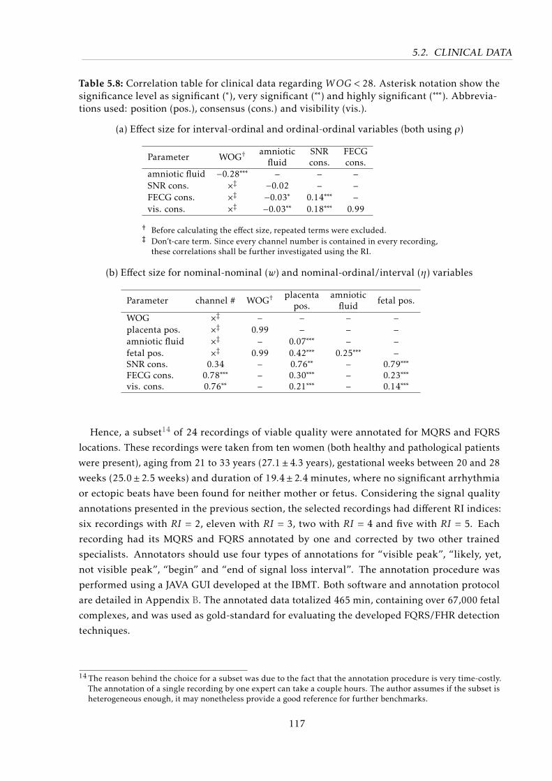
5.2. CLINICAL DATA
Table 5.8: Correlation table for clinical data regarding WOG < 28. Asterisk notation show thesignificance level as significant (∗), very significant (∗∗) and highly significant (∗∗∗). Abbrevia-tions used: position (pos.), consensus (cons.) and visibility (vis.).
(a) Effect size for interval-ordinal and ordinal-ordinal variables (both using ρ)
Parameter WOG† amnioticfluid
SNRcons.
FECGcons.
amniotic fluid −0.28∗∗∗ – – –SNR cons. ׇ −0.02 – –FECG cons. ׇ −0.03∗ 0.14∗∗∗ –vis. cons. ׇ −0.03∗∗ 0.18∗∗∗ 0.99
† Before calculating the effect size, repeated terms were excluded.‡ Don’t-care term. Since every channel number is contained in every recording,
these correlations shall be further investigated using the RI.
(b) Effect size for nominal-nominal (w) and nominal-ordinal/interval (η) variables
Parameter channel # WOG† placentapos.
amnioticfluid fetal pos.
WOG ׇ – – – –placenta pos. ׇ 0.99 – – –amniotic fluid ׇ – 0.07∗∗∗ – –fetal pos. ׇ 0.99 0.42∗∗∗ 0.25∗∗∗ –SNR cons. 0.34 – 0.76∗∗ – 0.79∗∗∗FECG cons. 0.78∗∗∗ – 0.30∗∗∗ – 0.23∗∗∗vis. cons. 0.76∗∗ – 0.21∗∗∗ – 0.14∗∗∗
Hence, a subset14 of 24 recordings of viable quality were annotated for MQRS and FQRS
locations. These recordings were taken from ten women (both healthy and pathological patients
were present), aging from 21 to 33 years (27.1± 4.3 years), gestational weeks between 20 and 28
weeks (25.0±2.5 weeks) and duration of 19.4±2.4 minutes, where no significant arrhythmia
or ectopic beats have been found for neither mother or fetus. Considering the signal quality
annotations presented in the previous section, the selected recordings had different RI indices:
six recordings with RI = 2, eleven with RI = 3, two with RI = 4 and five with RI = 5. Each
recording had its MQRS and FQRS annotated by one and corrected by two other trained
specialists. Annotators should use four types of annotations for “visible peak”, “likely, yet,
not visible peak”, “begin” and “end of signal loss interval”. The annotation procedure was
performed using a JAVA GUI developed at the IBMT. Both software and annotation protocol
are detailed in Appendix B. The annotated data totalized 465 min, containing over 67,000 fetal
complexes, and was used as gold-standard for evaluating the developed FQRS/FHR detection
techniques.
14 The reason behind the choice for a subset was due to the fact that the annotation procedure is very time-costly.The annotation of a single recording by one expert can take a couple hours. The author assumes if the subset isheterogeneous enough, it may nonetheless provide a good reference for further benchmarks.
117

5.3. CHAPTER SUMMARY
5.3 Chapter Summary
In this chapter, the two principal sources of data developed throughout this work were
presented. First, motivated by the lack of freely available abdECG databases, in cooperation
with the IBME (University of Oxford) a NIFECG simulator was developed, i.e. the so-called
FECGSYN (see Section 5.1.1). This versatile toolbox provides means for several types of non-
stationary abdominal mixtures and several pathophysiological scenarios. By making use of
the FECGSYN, a large open-access database was created (i.e. FECGSYNDB – see Section 5.1.2).
Second, together with the project partners at the University Hospital of Leipzig, a clinical
trial was conducted and resulted in n = 259 NIFECG recordings. The obtained clinical data
was statistically characterized in Section 5.2. The overall quality of NIFECG at early WOGs
(i.e. < 28 weeks) was shown to be fair. Particularly in this analysis, the dependence between
WOG and FECG amplitude was demonstrated. Indeed there is a strong attenuation of the
FECG around the 28-32 weeks, which is commonly associated with the vernix caseosa. Another
important factor discussed was the influence on electrode location and the power of fetal and
noise signals, where depending on the NIFECG application, a mixture of more and less distant
electrodes may be considered. Other influencing factors were also evaluated using a bivariate
analysis, however, the effects are not conclusive due to the modest size of the clinical dataset.
Further analysis should focus on multivariate analysis using a much larger dataset (i.e. at
least a couple thousand recordings). In the next chapter, the methods proposed in Chapter 4
are comprehensively benchmarked against several other extraction methods available in the
literature, using the produced data material here presented.
118

I only believe in statistics that I doctored myself
– origin unknown, often attributed to Winston S. Churchill
6Results for Data Analysis
In the previous chapters, several improvements on current extraction and detection tech-
niques for NIFECG analysis as well as valuable data were produced. In this chapter, these
suggested approaches are benchmarked in depth. In order to do so, the present chapter is
divided into two main sections, based on the type of analysis performed and data material
used. In Section 6.1, the simulated data (i.e. the FECGSYNDB - see Section 5.1.1) was used to
benchmark several extraction methods, in terms of FQRS detection and morphological fidelity of
NIFECG estimates. In Section 6.2, the best performing methods from each algorithmic category
(see Figure 3.4) were applied to the own clinical dataset collected throughout this work (see
Section 5.2).
6.1 Simulated Data
The application of simulated data for the purpose of characterizing NIFECG is particularly
important, since one can evaluate the different algorithms behavior in the presence of differ-
ent noise levels, non-stationary artefacts and pathophysiological events. In this section, the
FECGSYNDB was used to that end in an analog manner as in Andreotti et al. [18]. This database
comprises several pathophysiological scenarios, shown in Table 5.1.
6.1.1 Fetal QRS detection
This first experiment consisted of comparing different NIFECG extraction techniques in
terms of FQRS detection accuracy. As in [18], single-lead extraction methods were applied
to simulated leads 1, 8, 11, 14, 19, 22, 25, and 32 (see Fig. 5.2). In order to produce a fair
comparison between BSS and the remaining techniques (AM and TS), results are restricted
best outcomes amongst all leads/components. Gross statistics were calculated for evaluating
agreement (F1) and distance (MAE) measures (see Section 3.4.2). A case-by-case overview on
119
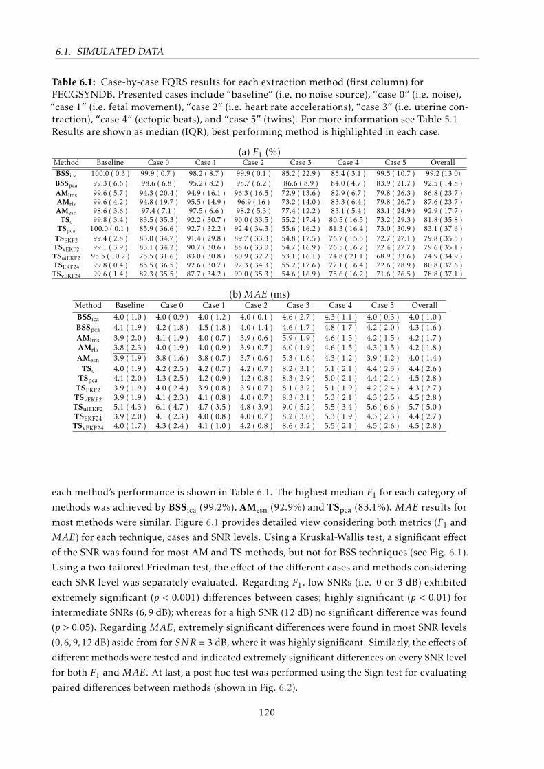
6.1. SIMULATED DATA
Table 6.1: Case-by-case FQRS results for each extraction method (first column) forFECGSYNDB. Presented cases include “baseline” (i.e. no noise source), “case 0” (i.e. noise),“case 1” (i.e. fetal movement), “case 2” (i.e. heart rate accelerations), “case 3” (i.e. uterine con-traction), “case 4” (ectopic beats), and “case 5” (twins). For more information see Table 5.1.Results are shown as median (IQR), best performing method is highlighted in each case.
(a) F1 (%)Method Baseline Case 0 Case 1 Case 2 Case 3 Case 4 Case 5 Overall
BSSica 100.0 ( 0.3 ) 99.9 ( 0.7 ) 98.2 ( 8.7 ) 99.9 ( 0.1 ) 85.2 ( 22.9 ) 85.4 ( 3.1 ) 99.5 ( 10.7 ) 99.2 (13.0)BSSpca 99.3 ( 6.6 ) 98.6 ( 6.8 ) 95.2 ( 8.2 ) 98.7 ( 6.2 ) 86.6 ( 8.9 ) 84.0 ( 4.7 ) 83.9 ( 21.7 ) 92.5 ( 14.8 )AMlms 99.6 ( 5.7 ) 94.3 ( 20.4 ) 94.9 ( 16.1 ) 96.3 ( 16.5 ) 72.9 ( 13.6 ) 82.9 ( 6.7 ) 79.8 ( 26.3 ) 86.8 ( 23.7 )AMrls 99.6 ( 4.2 ) 94.8 ( 19.7 ) 95.5 ( 14.9 ) 96.9 ( 16 ) 73.2 ( 14.0 ) 83.3 ( 6.4 ) 79.8 ( 26.7 ) 87.6 ( 23.7 )AMesn 98.6 ( 3.6 ) 97.4 ( 7.1 ) 97.5 ( 6.6 ) 98.2 ( 5.3 ) 77.4 ( 12.2 ) 83.1 ( 5.4 ) 83.1 ( 24.9 ) 92.9 ( 17.7 )
TSc 99.8 ( 3.4 ) 83.5 ( 35.3 ) 92.2 ( 30.7 ) 90.0 ( 33.5 ) 55.2 ( 17.4 ) 80.5 ( 16.5 ) 73.2 ( 29.3 ) 81.8 ( 35.8 )TSpca 100.0 ( 0.1 ) 85.9 ( 36.6 ) 92.7 ( 32.2 ) 92.4 ( 34.3 ) 55.6 ( 16.2 ) 81.3 ( 16.4 ) 73.0 ( 30.9 ) 83.1 ( 37.6 )
TSEKF2 99.4 ( 2.8 ) 83.0 ( 34.7 ) 91.4 ( 29.8 ) 89.7 ( 33.3 ) 54.8 ( 17.5 ) 76.7 ( 15.5 ) 72.7 ( 27.1 ) 79.8 ( 35.5 )TSvEKF2 99.1 ( 3.9 ) 83.1 ( 34.2 ) 90.7 ( 30.6 ) 88.6 ( 33.0 ) 54.7 ( 16.9 ) 76.5 ( 16.2 ) 72.4 ( 27.7 ) 79.6 ( 35.1 )TSuiEKF2 95.5 ( 10.2 ) 75.5 ( 31.6 ) 83.0 ( 30.8 ) 80.9 ( 32.2 ) 53.1 ( 16.1 ) 74.8 ( 21.1 ) 68.9 ( 33.6 ) 74.9 ( 34.9 )TSEKF24 99.8 ( 0.4 ) 85.5 ( 36.5 ) 92.6 ( 30.7 ) 92.3 ( 34.3 ) 55.2 ( 17.6 ) 77.1 ( 16.4 ) 72.6 ( 28.9 ) 80.8 ( 37.6 )TSvEKF24 99.6 ( 1.4 ) 82.3 ( 35.5 ) 87.7 ( 34.2 ) 90.0 ( 35.3 ) 54.6 ( 16.9 ) 75.6 ( 16.2 ) 71.6 ( 26.5 ) 78.8 ( 37.1 )
(b) MAE (ms)Method Baseline Case 0 Case 1 Case 2 Case 3 Case 4 Case 5 Overall
BSSica 4.0 ( 1.0 ) 4.0 ( 0.9 ) 4.0 ( 1.2 ) 4.0 ( 0.1 ) 4.6 ( 2.7 ) 4.3 ( 1.1 ) 4.0 ( 0.3 ) 4.0 ( 1.0 )BSSpca 4.1 ( 1.9 ) 4.2 ( 1.8 ) 4.5 ( 1.8 ) 4.0 ( 1.4 ) 4.6 ( 1.7 ) 4.8 ( 1.7 ) 4.2 ( 2.0 ) 4.3 ( 1.6 )AMlms 3.9 ( 2.0 ) 4.1 ( 1.9 ) 4.0 ( 0.7 ) 3.9 ( 0.6 ) 5.9 ( 1.9 ) 4.6 ( 1.5 ) 4.2 ( 1.5 ) 4.2 ( 1.7 )AMrls 3.8 ( 2.3 ) 4.0 ( 1.9 ) 4.0 ( 0.9 ) 3.9 ( 0.7 ) 6.0 ( 1.9 ) 4.6 ( 1.5 ) 4.3 ( 1.5 ) 4.2 ( 1.8 )AMesn 3.9 ( 1.9 ) 3.8 ( 1.6 ) 3.8 ( 0.7 ) 3.7 ( 0.6 ) 5.3 ( 1.6 ) 4.3 ( 1.2 ) 3.9 ( 1.2 ) 4.0 ( 1.4 )
TSc 4.0 ( 1.9 ) 4.2 ( 2.5 ) 4.2 ( 0.7 ) 4.2 ( 0.7 ) 8.2 ( 3.1 ) 5.1 ( 2.1 ) 4.4 ( 2.3 ) 4.4 ( 2.6 )TSpca 4.1 ( 2.0 ) 4.3 ( 2.5 ) 4.2 ( 0.9 ) 4.2 ( 0.8 ) 8.3 ( 2.9 ) 5.0 ( 2.1 ) 4.4 ( 2.4 ) 4.5 ( 2.8 )
TSEKF2 3.9 ( 1.9 ) 4.0 ( 2.4 ) 3.9 ( 0.8 ) 3.9 ( 0.7 ) 8.1 ( 3.2 ) 5.1 ( 1.9 ) 4.2 ( 2.4 ) 4.3 ( 2.7 )TSvEKF2 3.9 ( 1.9 ) 4.1 ( 2.3 ) 4.1 ( 0.8 ) 4.0 ( 0.7 ) 8.3 ( 3.1 ) 5.3 ( 2.1 ) 4.3 ( 2.5 ) 4.5 ( 2.8 )TSuiEKF2 5.1 ( 4.3 ) 6.1 ( 4.7 ) 4.7 ( 3.5 ) 4.8 ( 3.9 ) 9.0 ( 5.2 ) 5.5 ( 3.4 ) 5.6 ( 6.6 ) 5.7 ( 5.0 )TSEKF24 3.9 ( 2.0 ) 4.1 ( 2.3 ) 4.0 ( 0.8 ) 4.0 ( 0.7 ) 8.2 ( 3.0 ) 5.3 ( 1.9 ) 4.3 ( 2.3 ) 4.4 ( 2.7 )TSvEKF24 4.0 ( 1.7 ) 4.3 ( 2.4 ) 4.1 ( 1.0 ) 4.2 ( 0.8 ) 8.6 ( 3.2 ) 5.5 ( 2.1 ) 4.5 ( 2.6 ) 4.5 ( 2.8 )
each method’s performance is shown in Table 6.1. The highest median F1 for each category of
methods was achieved by BSSica (99.2%), AMesn (92.9%) and TSpca (83.1%). MAE results for
most methods were similar. Figure 6.1 provides detailed view considering both metrics (F1 and
MAE) for each technique, cases and SNR levels. Using a Kruskal-Wallis test, a significant effect
of the SNR was found for most AM and TS methods, but not for BSS techniques (see Fig. 6.1).
Using a two-tailored Friedman test, the effect of the different cases and methods considering
each SNR level was separately evaluated. Regarding F1, low SNRs (i.e. 0 or 3 dB) exhibited
extremely significant (p < 0.001) differences between cases; highly significant (p < 0.01) for
intermediate SNRs (6,9 dB); whereas for a high SNR (12 dB) no significant difference was found
(p > 0.05). Regarding MAE, extremely significant differences were found in most SNR levels
(0,6,9,12 dB) aside from for SNR = 3 dB, where it was highly significant. Similarly, the effects of
different methods were tested and indicated extremely significant differences on every SNR level
for both F1 and MAE. At last, a post hoc test was performed using the Sign test for evaluating
paired differences between methods (shown in Fig. 6.2).
120
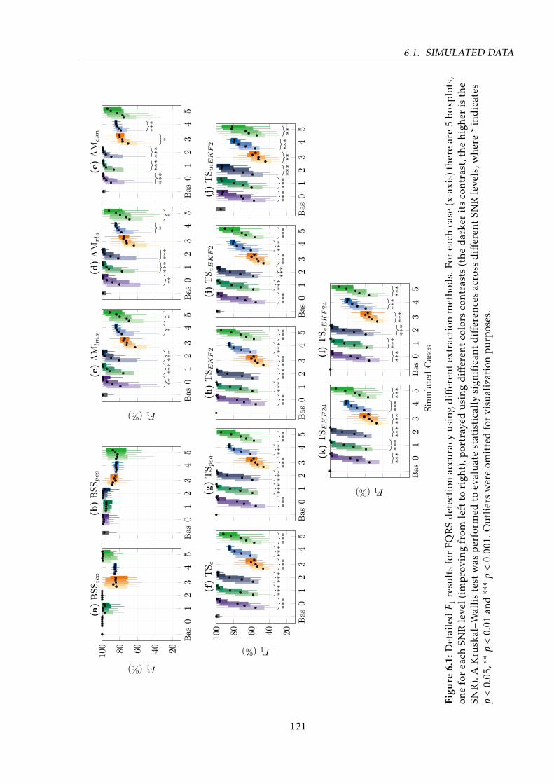
6.1. SIMULATED DATA
Bas
01
23
45
20406080100
F1(%)
(a)
BSS
ica
Bas
01
23
45
(b)
BSS
pca
Bas
01
23
45
****
***
**
*
F1(%)
(c)
AM
lms
Bas
01
23
45
****
***
**
*
(d)
AM
rls
Bas
01
23
45
***
***
***
*
***
(e)
AM
esn
Bas
01
23
45
20406080100
***
***
***
***
***
***
F1(%)
(f)
TS c
Bas
01
23
45
***
***
***
***
***
***
(g)
TS p
ca
Bas
01
23
45
***
***
***
***
***
***
(h)
TS E
KF2
Bas
01
23
45
***
***
***
***
***
***
(i)
TS v
EK
F2
Bas
01
23
45
***
***
***
****
***
(j)
TS u
iEK
F2
Bas
01
23
45
***
***
***
***
***
***
Sim
ulat
edC
ases
F1(%)
(k)
TS E
KF24
Bas
01
23
45
***
***
***
***
***
***
(l)
TS v
EK
F24
Figu
re6.
1:D
etai
ledF
1re
sult
sfo
rFQ
RS
det
ecti
onac
cura
cyu
sin
gd
iffer
ent
extr
acti
onm
etho
ds.
For
each
case
(x-a
xis)
ther
ear
e5
boxp
lots
,on
efo
rea
chSN
Rle
vel(
imp
rovi
ng
from
left
tori
ght)
,por
tray
edu
sin
gd
iffer
ent
colo
rsco
ntr
asts
(th
ed
arke
rit
sco
ntr
ast,
the
hig
her
isth
eSN
R).
AK
rusk
al–W
alli
ste
stw
asp
erfo
rmed
toev
alu
ate
stat
isti
call
ysi
gnifi
can
td
iffer
ence
sac
ross
diff
eren
tSN
Rle
vels
,wh
ere
*in
dic
ates
p<
0.05
,**p<
0.01
and
***p<
0.00
1.O
utl
iers
wer
eom
itte
dfo
rvi
sual
izat
ion
pu
rpos
es.
121
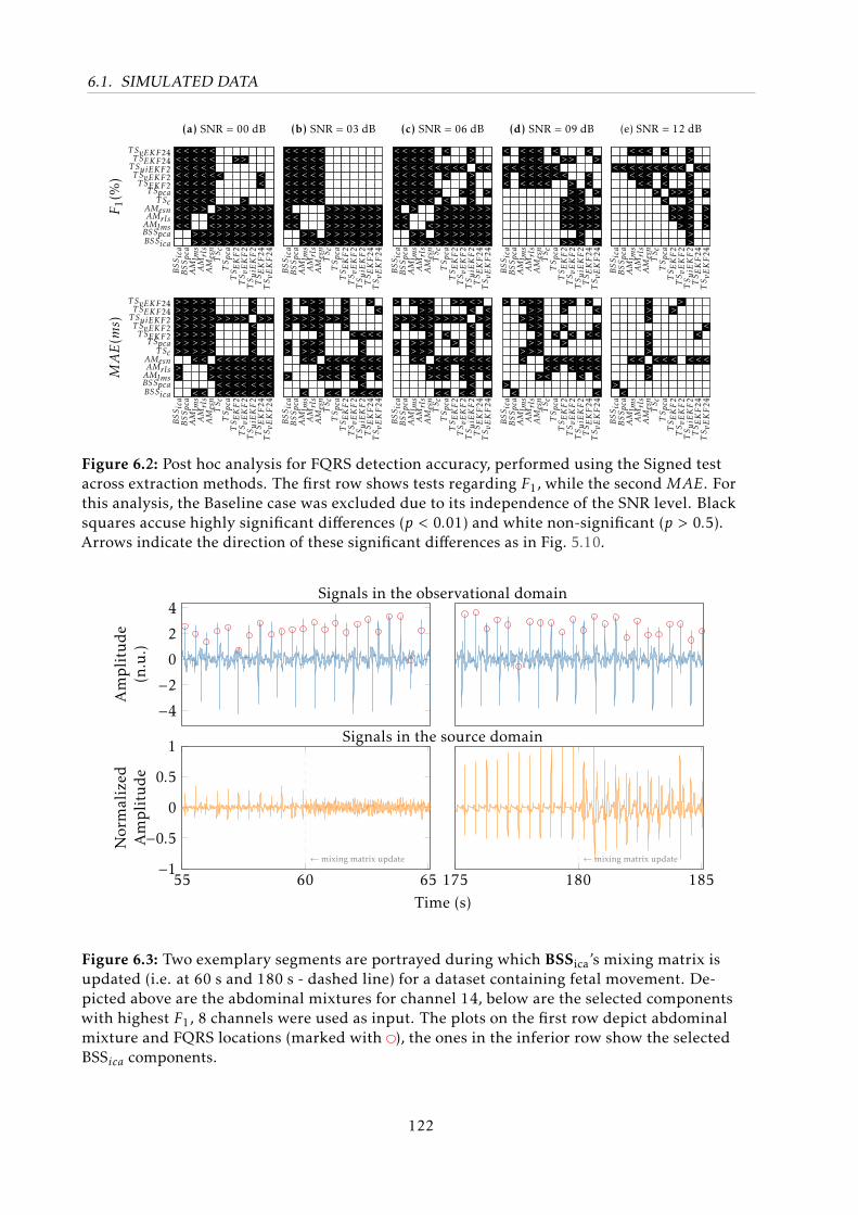
6.1. SIMULATED DATA
BSSica
BSSpca
AMlm
sAMrls
AMesn
TSc
TSpca
TSEKF2
TSvEKF2
TSuiE
KF2
TSEKF24
TSvEKF24
BSSicaBSSpcaAMlmsAMrlsAMesn
T ScT Spca
T SEKF2T SvEKF2T SuiEKF2T SEKF24
T SvEKF24 <<<<<<<<<<--
<<<<<<<<<<--
<<<<<<<>-->>
<<<<<<<>-->>
<<<<<<<-<<>>
---<--->>>>>
------->>>>>
->----->>>>>
->---->>>>>>
------->>>>>
---<<-->>>>>
------->>>>>
F1(%
)(a) SNR = 00 dB
BSSica
BSSpca
AMlm
sAMrls
AMesn
TSc
TSpca
TSEKF2
TSvEKF2
TSuiE
KF2
TSEKF24
TSvEKF24
<<<<<<<<<<--
<<<<<<<-<<--
<<<<<<<--->>
<<<<<<<--->>
<<<<<<<---->
------->>>>>
------->>>>>
------->>>>>
------->>>>>
------->>>>>
------->>>>>
------->>>>>
(b) SNR = 03 dB
BSSica
BSSpca
AMlm
sAMrls
AMesn
TSc
TSpca
TSEKF2
TSvEKF2
TSuiE
KF2
TSEKF24
TSvEKF24
<<<<<<<<<<--
<<<<<<<-<<--
<<<<<<<>-->>
<<<<<<<--->>
<<<<<<<--<->
--<-->->>>>>
<-<<--<>>>>>
--<---->>>>>
--<-->->>>>>
>>->>>>>>>>>
--<---->>>>>
--<-->->>>>>
(c) SNR = 06 dB
BSSica
BSSpca
AMlm
sAMrls
AMesn
TSc
TSpca
TSEKF2
TSvEKF2
TSuiE
KF2
TSEKF24
TSvEKF24
<-<<<-------
--<---------
<<<<<-------
<<<<<-------
<<<<<-------
--<<<-------
<-<<--------
->-<-->>>>->
->-->>>>>>->
----->>>>>>>
<--<<-->>>--
->--->->>>->
(d) SNR = 09 dB
BSSica
BSSpca
AMlm
sAMrls
AMesn
TSc
TSpca
TSEKF2
TSvEKF2
TSuiE
KF2
TSEKF24
TSvEKF24
--<---------
--<---------
<-<<--------
<-<<<-------
<-<<<-------
--<-->------
<-<<<-<-----
--<-->->>---
--<-->->>>--
>>->>>>>>>>>
--<---------
--<-->->>>--
(e) SNR = 12 dB
BSSica
BSSpca
AMlm
sAMrls
AMesn
TSc
TSpca
TSEKF2
TSvEKF2
TSuiE
KF2
TSEKF24
TSvEKF24
BSSicaBSSpcaAMlmsAMrlsAMesn
T ScT Spca
T SEKF2T SvEKF2T SuiEKF2T SEKF24
T SvEKF24 >>>>>>>->>--
>>>>>>>-----
>>>>>>><---<
>>>>>>><---<
>>>>>>>->>--
-->----<<<<<
-->----<<<<<
-->----<<<<<
-->----<<<<<
<<-<<<<<<<<<
-->----<<<<<
-->----<<<<<
MAE(m
s)
BSSica
BSSpca
AMlm
sAMrls
AMesn
TSc
TSpca
TSEKF2
TSvEKF2
TSuiE
KF2
TSEKF24
TSvEKF24
>>>>->>-->--
-->---------
>->>->><---<
>>>>->><----
>>>>>>>->>--
-->----<<<-<
-->----<<<-<
>>>>---<----
----<--<<<-<
----<<<<<<<<
>---<--<<--<
-<--<--<<<-<
BSSica
BSSpca
AMlm
sAMrls
AMesn
TSc
TSpca
TSEKF2
TSvEKF2
TSuiE
KF2
TSEKF24
TSvEKF24
>->>->>-----
-->---------
>->>->><----
>>>>->><----
>>>>>>>->>--
-->----<<<-<
-->-<--<<<-<
>->-->-<----
>->----<<<-<
<<-<<<<<<<<<
>->----<<---
-<><<--<<<-<
BSSica
BSSpca
AMlm
sAMrls
AMesn
TSc
TSpca
TSEKF2
TSvEKF2
TSuiE
KF2
TSEKF24
TSvEKF24
>--------->-
-----------<
>->---><----
>>>>->>-----
>>>>>>>-->--
-------<<<--
----<--<<---
>>->->-<----
>---<--<<---
-------<<<--
>---<--<<---
-<-<<--<<<-<
BSSica
BSSpca
AMlm
sAMrls
AMesn
TSc
TSpca
TSEKF2
TSvEKF2
TSuiE
KF2
TSEKF24
TSvEKF24
---------->-
-----------<
-------<----
-------<----
>>>->>>->>--
-------<----
-------<----
->-----<----
>-----------
-------<----
----<--<----
---<---<----
Figure 6.2: Post hoc analysis for FQRS detection accuracy, performed using the Signed testacross extraction methods. The first row shows tests regarding F1, while the second MAE. Forthis analysis, the Baseline case was excluded due to its independence of the SNR level. Blacksquares accuse highly significant differences (p < 0.01) and white non-significant (p > 0.5).Arrows indicate the direction of these significant differences as in Fig. 5.10.
−4−20
2
4
Amplitude
(n.u.)
55 60 65−1−0.5
0
0.5
1
←mixing matrix update
Normalized
Amplitude
175 180 185←mixing matrix update
Time (s)
Signals in the observational domain
Signals in the source domain
Figure 6.3: Two exemplary segments are portrayed during which BSSica’s mixing matrix isupdated (i.e. at 60 s and 180 s - dashed line) for a dataset containing fetal movement. De-picted above are the abdominal mixtures for channel 14, below are the selected componentswith highest F1, 8 channels were used as input. The plots on the first row depict abdominalmixture and FQRS locations (marked with ), the ones in the inferior row show the selectedBSSica components.
122
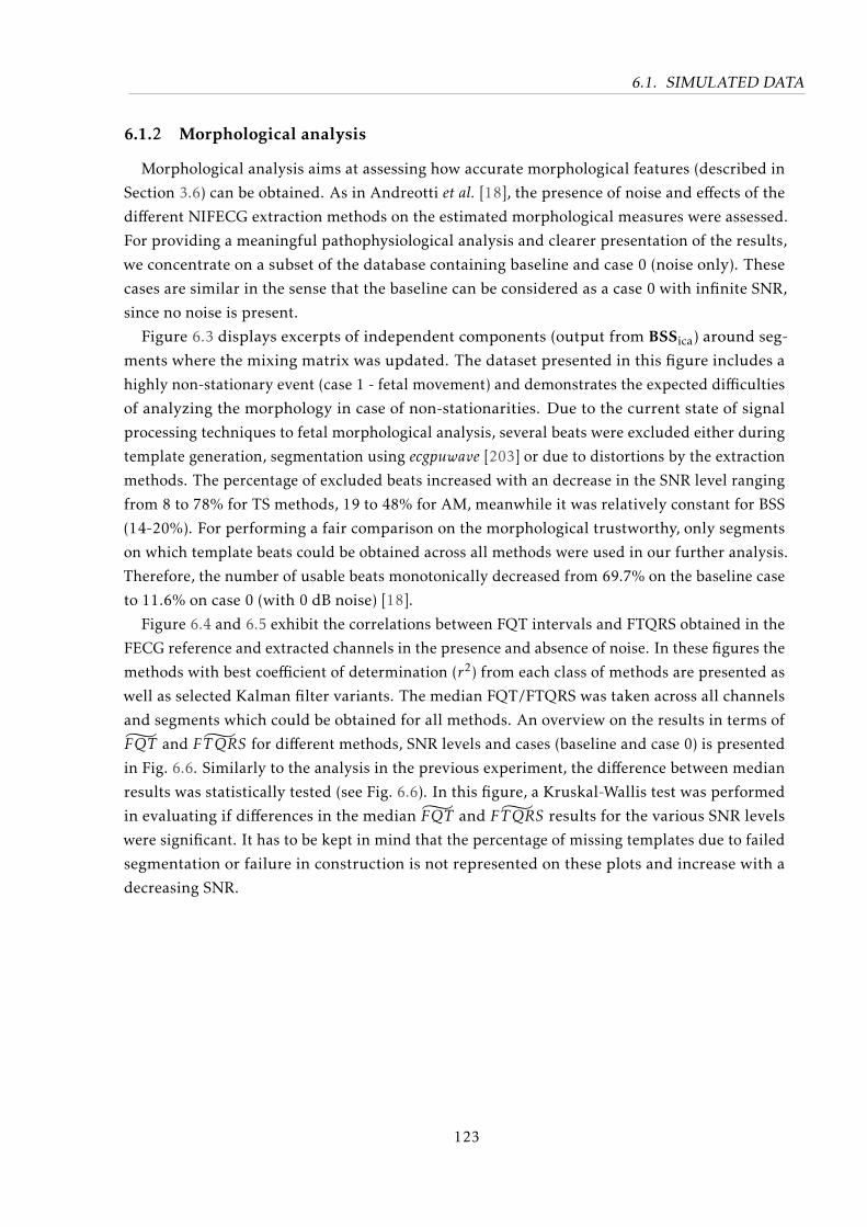
6.1. SIMULATED DATA
6.1.2 Morphological analysis
Morphological analysis aims at assessing how accurate morphological features (described in
Section 3.6) can be obtained. As in Andreotti et al. [18], the presence of noise and effects of the
different NIFECG extraction methods on the estimated morphological measures were assessed.
For providing a meaningful pathophysiological analysis and clearer presentation of the results,
we concentrate on a subset of the database containing baseline and case 0 (noise only). These
cases are similar in the sense that the baseline can be considered as a case 0 with infinite SNR,
since no noise is present.
Figure 6.3 displays excerpts of independent components (output from BSSica) around seg-
ments where the mixing matrix was updated. The dataset presented in this figure includes a
highly non-stationary event (case 1 - fetal movement) and demonstrates the expected difficulties
of analyzing the morphology in case of non-stationarities. Due to the current state of signal
processing techniques to fetal morphological analysis, several beats were excluded either during
template generation, segmentation using ecgpuwave [203] or due to distortions by the extraction
methods. The percentage of excluded beats increased with an decrease in the SNR level ranging
from 8 to 78% for TS methods, 19 to 48% for AM, meanwhile it was relatively constant for BSS
(14-20%). For performing a fair comparison on the morphological trustworthy, only segments
on which template beats could be obtained across all methods were used in our further analysis.
Therefore, the number of usable beats monotonically decreased from 69.7% on the baseline case
to 11.6% on case 0 (with 0 dB noise) [18].
Figure 6.4 and 6.5 exhibit the correlations between FQT intervals and FTQRS obtained in the
FECG reference and extracted channels in the presence and absence of noise. In these figures the
methods with best coefficient of determination (r2) from each class of methods are presented as
well as selected Kalman filter variants. The median FQT/FTQRS was taken across all channels
and segments which could be obtained for all methods. An overview on the results in terms of
FQT and ˜FTQRS for different methods, SNR levels and cases (baseline and case 0) is presented
in Fig. 6.6. Similarly to the analysis in the previous experiment, the difference between median
results was statistically tested (see Fig. 6.6). In this figure, a Kruskal-Wallis test was performed
in evaluating if differences in the median FQT and ˜FTQRS results for the various SNR levels
were significant. It has to be kept in mind that the percentage of missing templates due to failed
segmentation or failure in construction is not represented on these plots and increase with a
decreasing SNR.
123
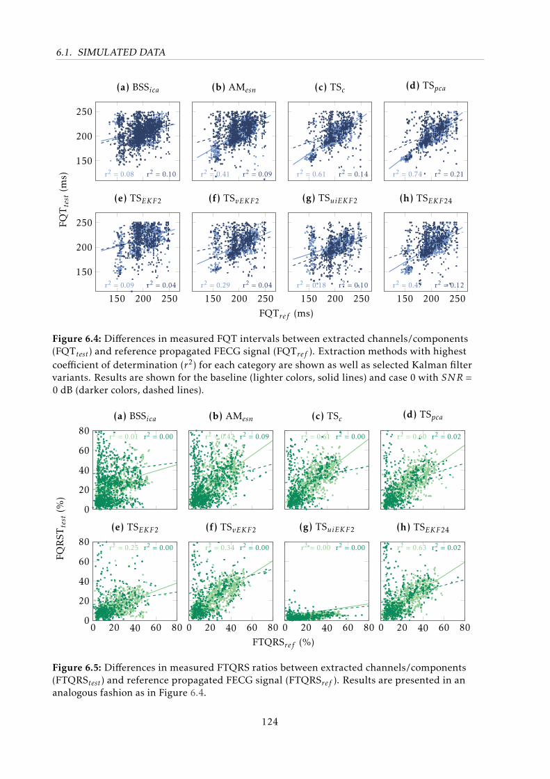
6.1. SIMULATED DATA
150
200
250
r2 = 0.08 r2 = 0.10
(a) BSSica
r2 = 0.41 r2 = 0.09
(b) AMesn
r2 = 0.61 r2 = 0.14
(c) TSc
r2 = 0.74 r2 = 0.21
(d) TSpca
150 200 250
150
200
250
r2 = 0.09 r2 = 0.04
FQTtest(m
s)
(e) TSEKF2
150 200 250r2 = 0.29 r2 = 0.04
FQTref (ms)
(f) TSvEKF2
150 200 250r2 = 0.18 r2 = 0.10
(g) TSuiEKF2
150 200 250r2 = 0.47 r2 = 0.12
(h) TSEKF24
Figure 6.4: Differences in measured FQT intervals between extracted channels/components(FQTtest) and reference propagated FECG signal (FQTref ). Extraction methods with highestcoefficient of determination (r2) for each category are shown as well as selected Kalman filtervariants. Results are shown for the baseline (lighter colors, solid lines) and case 0 with SNR =0 dB (darker colors, dashed lines).
0
20
40
60
80r2 = 0.01 r2 = 0.00
(a) BSSica
r2 = 0.42 r2 = 0.09
(b) AMesn
r2 = 0.61 r2 = 0.00
(c) TSc
r2 = 0.60 r2 = 0.02
(d) TSpca
0 20 40 60 800
20
40
60
80r2 = 0.25 r2 = 0.00
FQRST
test(%
)
(e) TSEKF2
0 20 40 60 80
r2 = 0.34 r2 = 0.00
FTQRSref (%)
(f) TSvEKF2
0 20 40 60 80
r2 = 0.00 r2 = 0.00
(g) TSuiEKF2
0 20 40 60 80
r2 = 0.63 r2 = 0.02
(h) TSEKF24
Figure 6.5: Differences in measured FTQRS ratios between extracted channels/components(FTQRStest) and reference propagated FECG signal (FTQRSref ). Results are presented in ananalogous fashion as in Figure 6.4.
124
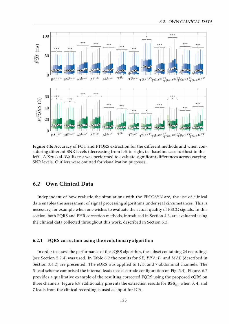
6.2. OWN CLINICAL DATA
BSSicaBSSpca AMlms
AMrls AMesn TScTSpca
TSEKF2
TSvEKF2
TSUIEKF2
TSEKF24
TSvEKF240
50
100
*** ***
*** *** ******
***
*
***
***
*** ***
FQT
(ms)
BSSicaBSSpca AMlms
AMrls AMesn TScTSpca
TSEKF2
TSvEKF2
TSUIEKF2
TSEKF24
TSvEKF240
20
40
60 ******
*** ***
*** ****** *
***
***
******
˜FTQRS
(%)
Figure 6.6: Accuracy of FQT and FTQRS extraction for the different methods and when con-sidering different SNR levels (decreasing from left to right, i.e. baseline case furthest to theleft). A Kruskal–Wallis test was performed to evaluate significant differences across varyingSNR levels. Outliers were omitted for visualization purposes.
6.2 Own Clinical Data
Independent of how realistic the simulations with the FECGSYN are, the use of clinical
data enables the assessment of signal processing algorithms under real circumstances. This is
necessary, for example when one wishes to evaluate the actual quality of FECG signals. In this
section, both FQRS and FHR correction methods, introduced in Section 4.3, are evaluated using
the clinical data collected throughout this work, described in Section 5.2.
6.2.1 FQRS correction using the evolutionary algorithm
In order to assess the performance of the eQRS algorithm, the subset containing 24 recordings
(see Section 5.2.4) was used. In Table 6.2 the results for SE, P P V , F1 and MAE (described in
Section 3.4.2) are presented. The eQRS was applied to 1, 3, and 7 abdominal channels. The
3-lead scheme comprised the internal leads (see electrode configuration on Fig. 5.4). Figure. 6.7
provides a qualitative example of the resulting corrected FQRS using the proposed eQRS on
three channels. Figure 6.8 additionally presents the extraction results for BSSica when 3, 4, and
7 leads from the clinical recording is used as input for ICA.
125
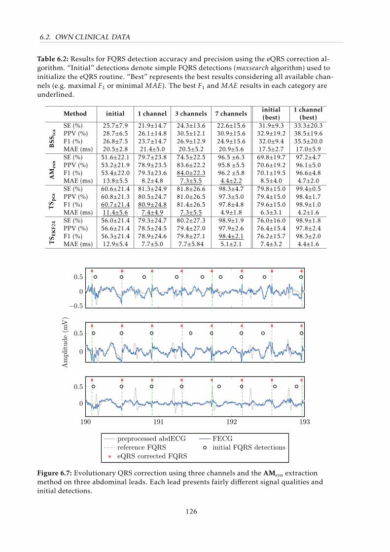
6.2. OWN CLINICAL DATA
Table 6.2: Results for FQRS detection accuracy and precision using the eQRS correction al-gorithm. “Initial” detections denote simple FQRS detections (maxsearch algorithm) used toinitialize the eQRS routine. “Best” represents the best results considering all available chan-nels (e.g. maximal F1 or minimal MAE). The best F1 and MAE results in each category areunderlined.
Method initial 1 channel 3 channels 7 channelsinitial(best)
1 channel(best)
SE (%) 25.7±7.9 21.9±14.7 24.3±13.6 22.6±15.6 31.9±9.3 33.3±20.3PPV (%) 28.7±6.5 26.1±14.8 30.5±12.1 30.9±15.6 32.9±19.2 38.5±19.6F1 (%) 26.8±7.5 23.7±14.7 26.9±12.9 24.9±15.6 32.0±9.4 35.5±20.0
BSS
ica
MAE (ms) 20.5±2.8 21.4±5.0 20.5±5.2 20.9±5.6 17.5±2.7 17.0±5.9SE (%) 51.6±22.1 79.7±23.8 74.5±22.5 96.5 ±6.3 69.8±19.7 97.2±4.7PPV (%) 53.2±21.9 78.9±23.5 83.6±22.2 95.8 ±5.5 70.6±19.2 96.1±5.0F1 (%) 53.4±22.0 79.3±23.6 84.0±22.3 96.2 ±5.8 70.1±19.5 96.6±4.8
AM
esn
MAE (ms) 13.8±5.5 8.2±4.8 7.3±5.5 4.4±2.2 8.5±4.0 4.7±2.0SE (%) 60.6±21.4 81.3±24.9 81.8±26.6 98.3±4.7 79.8±15.0 99.4±0.5PPV (%) 60.8±21.3 80.5±24.7 81.0±26.5 97.3±5.0 79.4±15.0 98.4±1.7F1 (%) 60.7±21.4 80.9±24.8 81.4±26.5 97.8±4.8 79.6±15.0 98.9±1.0T
S pca
MAE (ms) 11.4±5.6 7.4±4.9 7.3±5.5 4.9±1.8 6.3±3.1 4.2±1.6SE (%) 56.0±21.4 79.3±24.7 80.2±27.3 98.9±1.9 76.0±16.0 98.9±1.8PPV (%) 56.6±21.4 78.5±24.5 79.4±27.0 97.9±2.6 76.4±15.4 97.8±2.4F1 (%) 56.3±21.4 78.9±24.6 79.8±27.1 98.4±2.1 76.2±15.7 98.3±2.0
TS E
KF2
4
MAE (ms) 12.9±5.4 7.7±5.0 7.7±5.84 5.1±2.1 7.4±3.2 4.4±1.6
−0.5
0
0.5
0
0.5
Am
plit
ude
(mV
)
190 191 192 193
0
0.5
preprocessed abdECG FECGreference FQRS initial FQRS detectionseQRS corrected FQRS
Figure 6.7: Evolutionary QRS correction using three channels and the AMesn extractionmethod on three abdominal leads. Each lead presents fairly different signal qualities andinitial detections.
126
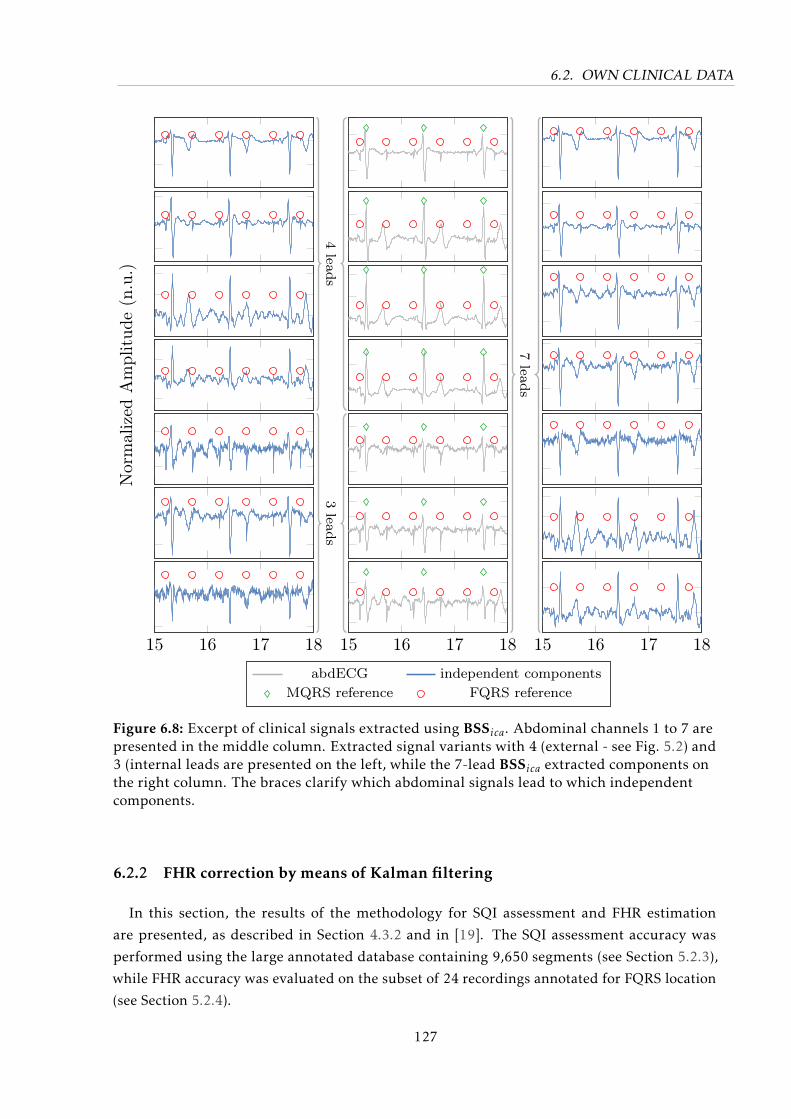
6.2. OWN CLINICAL DATA
Nor
mal
ized
Am
plit
ude
(n.u
.)
15 16 17 18 15 16 17 18Time (s)abdECG independent components
MQRS reference FQRS reference
15 16 17 18
4leads
3leads
7leads
Figure 6.8: Excerpt of clinical signals extracted using BSSica. Abdominal channels 1 to 7 arepresented in the middle column. Extracted signal variants with 4 (external - see Fig. 5.2) and3 (internal leads are presented on the left, while the 7-lead BSSica extracted components onthe right column. The braces clarify which abdominal signals lead to which independentcomponents.
6.2.2 FHR correction by means of Kalman filtering
In this section, the results of the methodology for SQI assessment and FHR estimation
are presented, as described in Section 4.3.2 and in [19]. The SQI assessment accuracy was
performed using the large annotated database containing 9,650 segments (see Section 5.2.3),
while FHR accuracy was evaluated on the subset of 24 recordings annotated for FQRS location
(see Section 5.2.4).
127
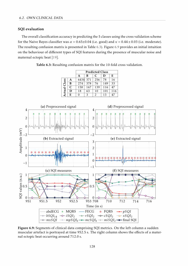
6.2. OWN CLINICAL DATA
SQI evaluation
The overall classification accuracy in predicting the 5 classes using the cross validation scheme
for the Naive Bayes classifier was α = 0.65±0.04 (i.e. good) and κ = 0.44± 0.03 (i.e. moderate).
The resulting confusion matrix is presented in Table 6.3). Figure 6.9 provides an initial intuition
on the behaviour of different types of SQI features during the presence of muscular noise and
maternal ectopic beat [19].
Table 6.3: Resulting confusion matrix for the 10-fold cross validation.
Predicted ClassA B C D E
Act
ual
Cla
ss A 6434 371 256 78 16B 274 378 76 149 33C 158 167 139 116 47D 18 63 10 101 116E 0 3 2 13 47
−2
0
2
4
−2
0
2
4
−1
0
1
Am
pli
tud
e(m
V)
−1
0
1
2
3
951 951.5 952 952.5 9530
0.5
1
Time (in s)
SQI
valu
es(n
.u.)
abdECG MQRS FECG FQRS pSQIbSQI14 iSQI2 rSQI2 cSQI2 xSQI2mxSQI mpSQIb mcSQIb miSQI2 final SQI
708 710 712 714 7160
0.5
1
(a) Preprocessed signal
(b) Extracted signal
(c) SQI measures
(d) Preprocessed signal
(e) Extracted signal
(f) SQI measures
Figure 6.9: Segments of clinical data comprising SQI metrics. On the left column a suddenmuscular artefact is portrayed at time 952.5 s. The right column shows the effects of a mater-nal ectopic beat occurring around 712.0 s.
128
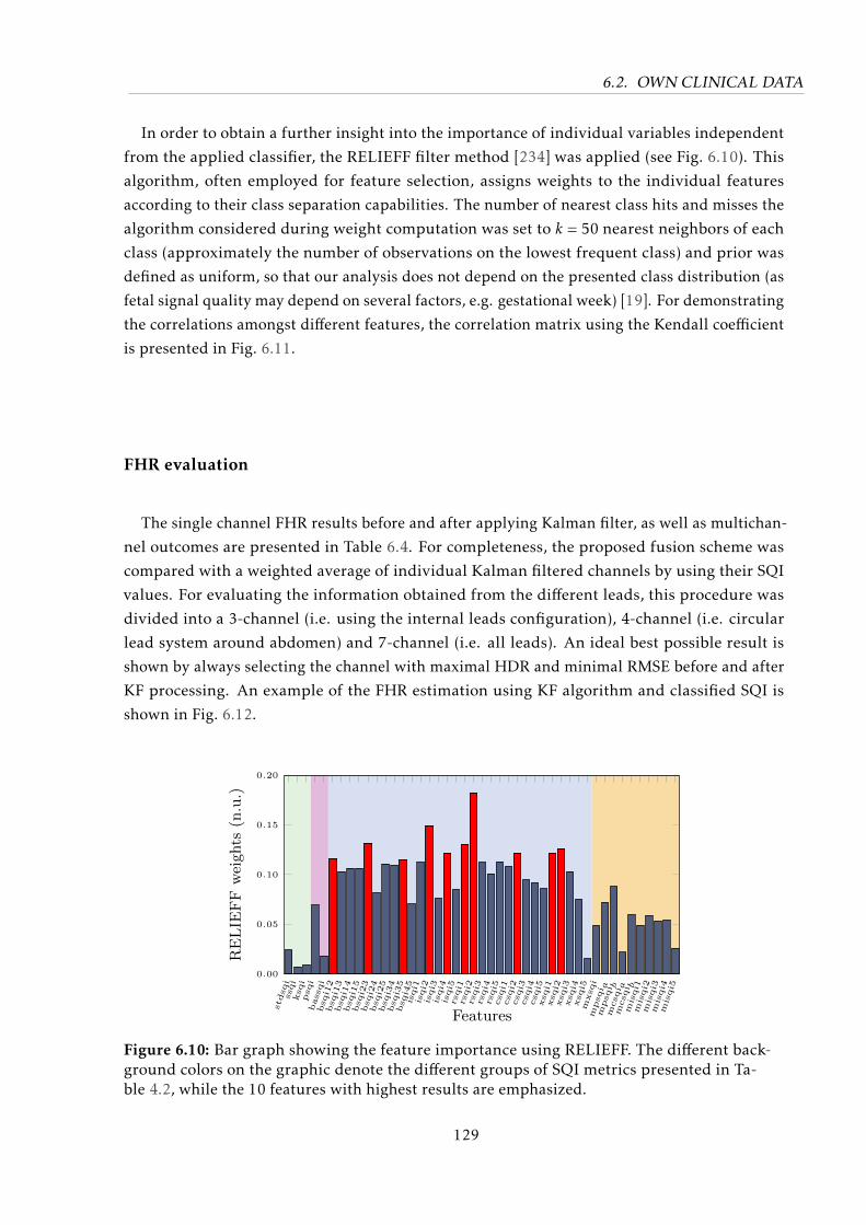
6.2. OWN CLINICAL DATA
In order to obtain a further insight into the importance of individual variables independent
from the applied classifier, the RELIEFF filter method [234] was applied (see Fig. 6.10). This
algorithm, often employed for feature selection, assigns weights to the individual features
according to their class separation capabilities. The number of nearest class hits and misses the
algorithm considered during weight computation was set to k = 50 nearest neighbors of each
class (approximately the number of observations on the lowest frequent class) and prior was
defined as uniform, so that our analysis does not depend on the presented class distribution (as
fetal signal quality may depend on several factors, e.g. gestational week) [19]. For demonstrating
the correlations amongst different features, the correlation matrix using the Kendall coefficient
is presented in Fig. 6.11.
FHR evaluation
The single channel FHR results before and after applying Kalman filter, as well as multichan-
nel outcomes are presented in Table 6.4. For completeness, the proposed fusion scheme was
compared with a weighted average of individual Kalman filtered channels by using their SQI
values. For evaluating the information obtained from the different leads, this procedure was
divided into a 3-channel (i.e. using the internal leads configuration), 4-channel (i.e. circular
lead system around abdomen) and 7-channel (i.e. all leads). An ideal best possible result is
shown by always selecting the channel with maximal HDR and minimal RMSE before and after
KF processing. An example of the FHR estimation using KF algorithm and classified SQI is
shown in Fig. 6.12.
stdsqi
ssqi
ksqi
psqi
bassqi
bsqi1
2bsqi1
3bsqi1
4bsqi1
5bsqi2
3bsqi2
4bsqi2
5bsqi3
4bsqi3
5bsqi4
5isqi1
isqi2
isqi3
isqi4
isqi5
rsqi1
rsqi2
rsqi3
rsqi4
rsqi5
csqi1
csqi2
csqi3
csqi4
csqi5
xsqi1
xsqi2
xsqi3
xsqi4
xsqi5
mxsqi
mpsqi a
mpsqi b
mcsqi a
mcsqi b
misqi1
misqi2
misqi3
misqi4
misqi5
0.00
0.05
0.10
0.15
0.20
Features
RELIE
FF
weights
(n.u.)
Figure 6.10: Bar graph showing the feature importance using RELIEFF. The different back-ground colors on the graphic denote the different groups of SQI metrics presented in Ta-ble 4.2, while the 10 features with highest results are emphasized.
129
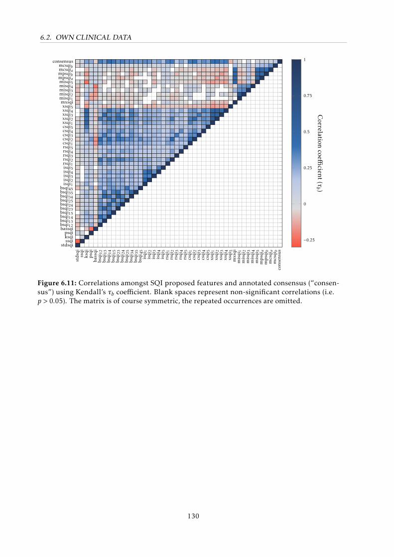
6.2. OWN CLINICAL DATA
stdsqi
ssqi
ksqi
psqi
bassqi
bsqi
12bsqi
13bsqi
14bsqi
15bsqi
23bsqi
24bsqi
25bsqi
34bsqi
35bsqi
45isqi
1isqi
2isqi
3isqi
4isqi
5rsqi
1rsqi
2rsqi
3rsqi
4rsqi
5csqi
1csqi
2csqi
3csqi
4csqi
5xsqi
1xsqi
2xsqi
3xsqi
4xsqi
5mxsqi
misqi
1misqi
2misqi
3misqi
4misqi
5mpsqi a
mpsqi b
mcsqia
mcsqib
cons
ensu
s
stdsqissqiksqipsqi
bassqibsqi12bsqi13bsqi14bsqi15bsqi23bsqi24bsqi25bsqi34bsqi35bsqi45isqi1isqi2isqi3isqi4isqi5rsqi1rsqi2rsqi3rsqi4rsqi5csqi1csqi2csqi3csqi4csqi5xsqi1xsqi2xsqi3xsqi4xsqi5mxsqimisqi1misqi2misqi3misqi4misqi5mpsqiampsqibmcsqiamcsqib
consensus
−0.25
0
0.25
0.5
0.75
1
Correlation
coefficient
(τb )
Figure 6.11: Correlations amongst SQI proposed features and annotated consensus (“consen-sus”) using Kendall’s τb coefficient. Blank spaces represent non-significant correlations (i.e.p > 0.05). The matrix is of course symmetric, the repeated occurrences are omitted.
130
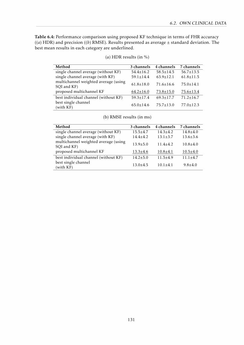
6.2. OWN CLINICAL DATA
Table 6.4: Performance comparison using proposed KF technique in terms of FHR accuracy((a) HDR) and precision ((b) RMSE). Results presented as average ± standard deviation. Thebest mean results in each category are underlined.
(a) HDR results (in %)
Method 3 channels 4 channels 7 channelssingle channel average (without KF) 54.4±16.2 58.5±14.5 56.7±13.5single channel average (with KF) 59.1±14.4 63.9±12.1 61.8±11.5multichannel weighted average (usingSQI and KF) 61.8±18.0 71.6±16.6 75.0±14.1
proposed multichannel KF 64.2±16.0 73.8±15.0 75.6±13.4best individual channel (without KF) 59.3±17.4 69.3±17.7 71.2±16.7best single channel(with KF) 65.0±14.6 75.7±13.0 77.0±12.3
(b) RMSE results (in ms)
Method 3 channels 4 channels 7 channelssingle channel average (without KF) 15.5±4.7 14.3±4.2 14.8±4.0single channel average (with KF) 14.4±4.2 13.1±3.7 13.6±3.6multichannel weighted average (usingSQI and KF) 13.9±5.0 11.4±4.2 10.8±4.0
proposed multichannel KF 13.3±4.6 10.8±4.1 10.5±4.0best individual channel (without KF) 14.2±5.0 11.5±4.9 11.1±4.7best single channel(with KF) 13.0±4.5 10.1±4.1 9.8±4.0
131
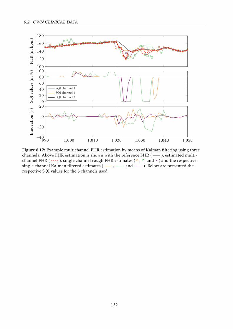
6.2. OWN CLINICAL DATA
100
120
140
160
180FH
R(inbp
m)
020406080
100
SQIva
lues
(in%)
SQI channel 1SQI channel 2SQI channel 3
990 1,000 1,010 1,020 1,030 1,040 1,050−40
−20
0
20
Inno
vation
(ν)
Figure 6.12: Example multichannel FHR estimation by means of Kalman filtering using threechannels. Above FHR estimation is shown with the reference FHR ( ), estimated multi-channel FHR ( ), single channel rough FHR estimates ( , and ) and the respectivesingle channel Kalman filtered estimates ( , and ). Below are presented therespective SQI values for the 3 channels used.
132

So, if she weighs the same as a duck, then she’s made of wood.
And therefore... A WITCH!
– Monty Python and the Holy Grail (1975)
7Discussion and Prospective
As demonstrated throughout this work, NIFECG is a topic of ongoing research, whose
promising initial results have culminated on the emergence of a first generation of commercial
monitors (described in Section 3.2.2). However, there are several important aspects that need
to be further investigated before NIFECG becomes a clinical standard in continuous fetal
monitoring (see Chapter 2 and Behar et al. [51] for details). In the next sections, the main results
of this thesis as well as suggestions for future research are discussed.
7.1 Data Availability
The currently available databases for NIFECG analysis were presented in Section 3.2.4. As
described in this section, these datasets are very limited in size and spectrum of pathophysio-
logical conditions they contain. With the purpose of making NIFECG analysis more accessible,
objective and reproducible, in Chapter 5 the FECGSYN simulator (see Behar et al. [50]) and
FECGSYNDB (see Andreotti et al. [18]) simulated database were developed in this work. This
large simulated database can be used to train extraction and detection algorithms with a wide
number of non-stationary events (see Section 5.1), which in clinical settings are difficult to
collect/quantify. The increasing number of researchers using the developed platforms (and
consequent citations to the respective work [18, 50]) are proof of their usefulness.
Still, to demonstrate NIFECG’s efficacy, multi-center randomized clinical trials are necessary.
With respect to reproducibility, a more comprehensive open access medical database of NIFECG
signals is highly desirable (as described in [51]). Similar to the largely available adult QT [98,
239] and arrhythmia databases [286], such dataset would to allow researchers to rapidly discredit
unreliable clinical metrics such as the recent case of FTQRS in invasive FECG monitoring
(presented in Section 3.1) and allow that automated approaches to analyze FHR/FHRV tracings
are compared. This clinical trial/database should comprise different gestational ages (to capture
133
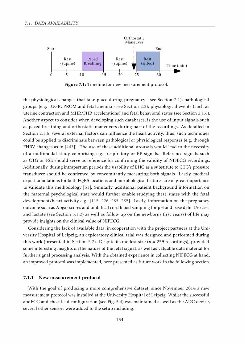
7.1. DATA AVAILABILITY
Rest(supine)
PacedBreathing
OrthostaticManeuver
0 5 10 15 20 25 30
Time (min)
Start End
Rest(supine)
Rest(sitted)
Figure 7.1: Timeline for new measurement protocol.
the physiological changes that take place during pregnancy - see Section 2.1), pathological
groups (e.g. IUGR, PROM and fetal anemia - see Section 2.2), physiological events (such as
uterine contraction and MHR/FHR accelerations) and fetal behavioral states (see Section 2.1.6).
Another aspect to consider when developing such databases, is the use of input signals such
as paced breathing and orthostatic maneuvers during part of the recordings. As detailed in
Section 2.1.6, several external factors can influence the heart activity, thus, such techniques
could be applied to discriminate between pathological or physiological responses (e.g. through
FHRV changes as in [443]). The use of these additional arousals would lead to the necessity
of a multimodal study comprising e.g. respiratory or BP signals. Reference signals such
as CTG or FSE should serve as reference for confirming the validity of NIFECG recordings.
Additionally, during intrapartum periods the usability of EHG as a substitute to CTG’s pressure
transducer should be confirmed by concomitantly measuring both signals. Lastly, medical
expert annotations for both FQRS locations and morphological features are of great importance
to validate this methodology [51]. Similarly, additional patient background information on
the maternal psychological state would further enable studying these states with the fetal
development/heart activity e.g. [115, 226, 285, 285]. Lastly, information on the pregnancy
outcome such as Apgar scores and umbilical cord blood sampling for pH and base deficit/excess
and lactate (see Section 3.1.2) as well as follow up on the newborns first year(s) of life may
provide insights on the clinical value of NIFECG.
Considering the lack of available data, in cooperation with the project partners at the Uni-
versity Hospital of Leipzig, an exploratory clinical trial was designed and performed during
this work (presented in Section 5.2). Despite its modest size (n = 259 recordings), provided
some interesting insights on the nature of the fetal signal, as well as valuable data material for
further signal processing analysis. With the obtained experience in collecting NIFECG at hand,
an improved protocol was implemented, here presented as future work in the following section.
7.1.1 New measurement protocol
With the goal of producing a more comprehensive dataset, since November 2014 a new
measurement protocol was installed at the University Hospital of Leipzig. Whilst the successful
abdECG and chest lead configuration (see Fig. 5.4) was maintained as well as the ADC device,
several other sensors were added to the setup including:
134
7.1. DATA AVAILABILITY
• respiration belt: placed around thorax on the breast area;
• finger PPG sensor: applied on the right hand’s index finger;
• continuous blood pressure: using the Finometer MIDI (Finapres Medical Systems B.V.,
Amsterdam, Netherlands), applied on the left middle finger as specified by manufacturer.
The Finometer was calibrate before each recording and auto-calibration took place on
every couple seconds;
• hand-held Doppler: model AngelSounds JPD-100S (Jumper Medical, Shenzhen, China),
the probe was carefully positioned and hold by recording expert during the whole record-
ing while attempting to minimize movement and contact with the abdominal electrodes,
while maximizing the audible FHR sound.
In order to make the recordings more reproducible, a GUI was developed to guide the
medical expert throughout the measurement. This GUI was developed in JAVA programming
language and is described in Appendix C. In order to observe fetal cardiac response to external
arousals, the novel recording protocol consisted of periods of rest and the performance of both
paced breathing and orthostatic maneuvers (see Figure 7.1). Based on [443] a breathing rate of
20 cycles/min was chosen, using the aforementioned GUI audible cues were given to “breath
in” and “breath out” during a 5 min phase. Obviously, when dealing with pregnant women
(often unwell patients) these maneuvers have to be as quotidian as possible. For this reason, as
orthostatic maneuver the choice was for natural everyday movement, where the subjects were
asked to change their position from supine into sitting position themselves.
On a preliminary study [276] comprising 16 initial recordings, no statistical difference
between the mean FHR for spontaneous and pace breathing was found. However, this may be
attribute to 1) the choice of breathing rate, which was found to be very similar to the normal
rate for pregnant women (generally for adults at rest is around 13 cycles/min, but higher for
pregnant women); and 2) the small number and general low quality of the available recordings
(ca. 20.5 % had visible FQRS peaks). Another feasibility study [415] using the same dataset has
shown a significant change in BP despite the subtleness of the performed maneuver. Similarly, a
significance test expressive short-term changes (≈ 1 min after maneuver) and long-term changes
(≈ 3 min after maneuver) on the average FHR. An unexpected result was the clear decrease
on FECG quality that reduced FQRS visibility from 20.5 % (before maneuver) to 4.4 % (after
maneuver). This may be attributed to changes on the position of maternal organs and strong
muscular artefact due to movement. However, as in the previous study, due to the limited data
available the results have to be considered with care. Nonetheless, this initial knowledge is
an important preliminary step before for the actual clinical trial that should follow. With the
limitations of current databases in mind, this data should be prospectively made freely available
at Physionet [161].
135
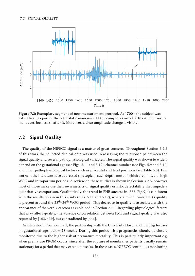
7.2. SIGNAL QUALITY
1400 1450 1500 1550 1600 1650 1700 1750 1800 1850 1900 1950 2000 2050
−2
0
2
Time (s)
Amplitude(m
V)
1400 1450 1500 1550 1600 1650 1700 1750 1800 1850 1900 1950 2000 2050
−2
0
2
Time (s)
Amplitude(m
V)
1400 1450 1500 1550 1600 1650 1700 1750 1800 1850 1900 1950 2000 2050
−2
0
2
Time (s)
Amplitude(m
V)
Figure 7.2: Exemplary segment of new measurement protocol. At 1700 s the subject wasasked to sit as part of the orthostatic maneuver. FECG complexes are clearly visible prior tomaneuver, but less so after it. Moreover, a clear amplitude change is visible.
7.2 Signal Quality
The quality of the NIFECG signal is a matter of great concern. Throughout Section 5.2.3
of this work the collected clinical data was used in assessing the relationships between the
signal quality and several pathophysiological variables. The signal quality was shown to widely
depend on the gestational age (see Figs. 5.11 and 5.12), channel number (see Figs. 5.9 and 5.10)
and other pathophysiological factors such as placental and fetal positions (see Table 5.8). Few
works in the literature have addressed this topic in such depth, most of which are limited to high
WOG and intrapartum periods. A review on these studies is shown in Section 3.2.5, however
most of those make use their own metrics of signal quality or FHR detectability that impede a
quantitative comparison. Qualitatively, the trend in FHR success in [333, Fig.9] is consistent
with the results obtain in this study (Figs. 5.11 and 5.12), where a much lower FECG quality
is present around the 28th-36th WOG period. This decrease in quality is associated with the
appearance of the vernix caseosa as explained in Section 2.1.3. Regarding physiological factors
that may affect quality, the absence of correlation between BMI and signal quality was also
reported by [163, 439], but contradicted by [446].
As described in Section 5.2.2, the partnership with the University Hospital of Leipzig focuses
on gestational ages below 28 weeks. During this period, risk pregnancies should be closely
monitored due to the higher risk of premature mortality. This is particularly important e.g.
when premature PROM occurs, since after the rupture of membranes patients usually remain
stationary for a period that may extend to weeks. In these cases, NIFECG continuous monitoring
136
7.2. SIGNAL QUALITY
could significantly improve patient’s comfort. However, concerns about the quality of the
obtained NIFECG have hampered such approach. In an attempt to better characterize such
signals, the analysis presented in Section 5.2.3 is partially direct to this period (shown in
Table 5.8). For instance, placental position was found to correlate with both SNR and FECG
amplitude, which could be due to its higher relative permittivity. Fetal presentation is also
important, since it goes along with electrode configuration, therefore, with signal quality. In this
study a strong and highly significant dependency was found between fetal position and SNR
ratio and fetuses in vertex position have shown higher FECG amplitude. Despite our dataset
being larger than that of most the referred studies, the described statistical results must be
considered with care since the population involved in this exploratory study is limited for the
broad spectrum of pathophysiological conditions of its patients. The author re-iterates the
importance of a large randomized clinical study to verify the true nature of these relationships.
Aside from the aforementioned associations, the inter-subject dependency should be regarded 1.
Similarly, a more comprehensive multivariate analysis could provide insights on the associations
between multiple variables e.g. the influence fetal position coupled with electrode configuration
in the resulting recording quality.
Electrode placement and inter-electrode distance is an important topic that remains virtually
unexplored in the literature (addressed in this work’s Section 3.2.3). In this thesis, the electrode
configuration was shown to have a significant effect on both abdominal signal SNR and FECG
content. In Figures. 5.9 and 5.10 it is clear the difference on signal quality for the different leads
used in this work. The inter-electrode distance was shown to play a large role on the signal
quality, where a trade-off between FECG amplitude and SNR exists. For further works, the
combination of shorter and larger leads is recommended (e.g. 2,6-8 – see Fig. 5.4), in order to
maximize the chances of obtaining usable NIFECG signals.
With the objective of providing automated means of assessing signal quality in NIFECG
recordings, in Section 4.3.2 several SQI metrics were introduced in this work. These metrics,
were then applied using a Naive Bayes classifier for estimating the signal quality of 5 s segments
of extracted NIFECG data. With respect to the proposed Naive Bayes classifier, good classifica-
tion results were obtained during cross validation using Krippendorff’s α coefficient, i.e. the
most suitable metric considering the ordinal dataset used. Meanwhile, Cohen’s κ produces
moderate results, since it is a nominal agreement measure. Visual inspection of the confusion
matrix (Table 6.3) confirms that most false classifications fall within neighboring classes. It
is important to mention that the Naive Bayes classifier assumes the features to be normally
distributed and conditionally independent given a class, which is a strong assumption that does
not hold for our data. Nevertheless, studies have shown [118] that Bayesian classifiers perform
quite well in practice even when attribute dependencies are present. Furthermore, its use is
justified by the transparent conversion from discrete to continuous-valued classification results,
which was necessary for the further processing. The underlying class distribution (see Fig. 4.10)
is expected to impact the trained classifier in terms of prior class probability. The assumption
1 In this work, different measurements from the same subjects were regarded as independent, which may be anerroneous assumption.
137
7.2. SIGNAL QUALITY
of uniform class distribution was relevant for improving the generalization potential of this
classifier. Unfortunately, there is no annotated clinical database currently available to serve as a
standard for comparing our classification results and provide further insights into the signal
quality distribution [19].
As it can be seen from Fig. 6.10, it is evident that time and frequency metrics (see Table 4.2
showed little importance, which can be explained by the well-known similarities and spectral
overlap between abdominal ECG/MECG/FECG. Detection-based algorithms such as bSQI ,
rSQI , cSQI and xSQI (particularly when using maxsearch or jQRS detectors) were relevant.
While applying bSQI , it is particularly important to use a combination of a more and other
less predictive detector, e.g. jQRS/gqrs (similar to the results obtained in [211]). This result
goes along with the author’s previous works and top scoring entry on the PCINCC 2013 [20],
where features like cSQI , xSQI , and rSQI were responsible for accurate FQRS detections.
The proposed FECG-specific features (latter group in Fig. 6.10) showed modest importance.
Amongst these, mpSQIb was deemed as most important by RELIEFF in the latter SQI category
(see Fig. 6.10) that can be confirmed its moderate reaction to the presence of noise (on Fig. 6.9).
From Fig. 6.11 the correlations amongst some features are made evident, e.g. between rSQI1,
rSQI2, and rSQI3. Interestingly, FECG-specific features show a different direction of correlation,
compared to the other three groups of SQI approaches. The consensus itself, appears to be
uncorrelated with most metrics, except the FECG-specific approaches. This is explained by
the fact that RELIEFF weights and Kendall correlation coefficients make different nonlinear
transformations to the provided variables. The first evaluates the euclidean distance between
available classes for for the nearest-hit/miss in the feature-space, while the second ranks its
variables and compares the number of concordant and discordant pairs of variables (features
against consensus). Indeed, feature selection is a comprehensive topic which extrapolates the
scope of this work. As future work, the author suggests the analysis of these interdependencies
for e.g. to reduce the information redundancy from similar SQI metrics.
In Fig. 6.9 (a)-(c) it is visible that most features produce lower values in the presence of
muscular noise, while iSQI2 and some FECG-specific indices (i.e. mpSQIb,mcSQIb andmiSQI2)
counter-intuitively output higher values. Nevertheless, the resulting continuous-valued SQI
showed to be very sensitive to such artefacts. On the other hand, Fig. 6.9 (d)-(f) portrays a
drawback of the proposed approach, where the estimated SQI value is larger during a maternal
ectopic beat. This is caused by the MECG large amplitude residual left over from a unsatisfactory
extraction procedure. In this case, iSQI2 output considerably higher values, since the ectopic
maternal complex still present in the residuals is expected to be detected on every lead. For
solving this problem, one may for example introduce SQI metrics similar to the fetal cSQI that
focus on the morphological consistency of the maternal signal.
Despite being larger than most datasets available in the specific literature, one limitation
of our data is the large disparity on the number of observations on each signal quality class,
where most data has low signal quality (see Figure 4.10). Another limiting factor is the fact
that the quality of the NI-FECG recordings was annotated using abdominal recordings (prior
to extraction of the FECG), while most proposed SQI metrics are based on the extracted FECG
138
7.3. EXTRACTION METHODS
signals. Consequently, the training data depends on the extraction method used, which is
not ideal. Nevertheless, the method of choice for this analysis, i.e. TSpca, is simple enough
and should not produce any major distortion between the annotated and extracted signals.
Furthermore, the author recognizes that the defined overall consensus (see Table 5.6) is a
subjective concept and may be sub-optimal. However, it was a necessary step for the analysis.
Another possibility would be to have two separate sets of SQIs and classifiers, one dealing with
the signal SNR and another with the amplitude of the FQRS peaks. Regarding the length of the
segments used in this work, although some SQI algorithms may benefit from longer segments
(e.g. for building FECG templates or estimating spectral content) the 5 s interval was considered
as appropriate for the trade-off between window length and online capability of the proposed
algorithm. As described in Section 3.5, Doppler ultrasound approaches currently use a similar
3.75 s interval.
All in all, the proposed SQI metrics are able to reflect changes in signal quality for NIFECG
recordings. The developed routines were released as part of the FECGSYN toolbox [50] under a
GNU GPL open-source license [19]. As mentioned in Section 4.3.2, such automated estimates for
FECG signal quality are indispensable for improving signal processing algorithm’s specificity.
In this work, these metrics were used in FQRS correction (Section 4.3.1) and FHR estimation
(Section 4.3.2). Both these approaches are further discussed in Section 7.4. Future uses for such
SQIs are for instance in channel/component selection, e.g. when applying BSSica extraction.
7.3 Extraction Methods
Despite the large number of NIFECG extraction methods proposed in the literature (see
Section 3.3.1), very few studies have in fact made their code available. The PCINC 2013
promoted a considerable advance in the field by making a dataset and evaluation algorithms
freely available, while some participants could voluntarily open-source their own code. In
this work, in cooperation with the IBME, the author developed a realistic open-source FECG
simulator and toolbox for NIFECG signal processing and analysis (i.e. the FECGSYN Behar
et al. [50]). The toolbox was further applied in generating a comprehensive simulated dataset,
totalizing 145.8 hours of multichannel data and 1.1 million fetal peaks (i.e. the FECGSYNDB
[18]). These two well-defined tools, are currently the largest open-source collection of NIFECG
extraction algorithms and data known to the author, which allow reproducible research in the
field. Throughout this work, these benefits were enjoyed and culminated in a wide-ranging and
well-defined benchmark of state-of-the-art (Section 3.3.1) and newly proposed EKF approaches
(Section 4.2).
From Fig. 6.1 and Table 6.1, it is clear that under ideal circumstances (i.e. when the best
available lead/component is known) BSS techniques (especially BSSica) outperforms all other
approaches. Meanwhile, TSpca and AMesn obtained the best results in their respective categories
(similar findings for the AM category using real data were presented in [52, 258]). BSS methods
have showed to be robust to the presence of noise in any level, while AM and TS techniques are
extremely susceptible to noise. MAE results were very similar for all methods, notwithstanding,
139
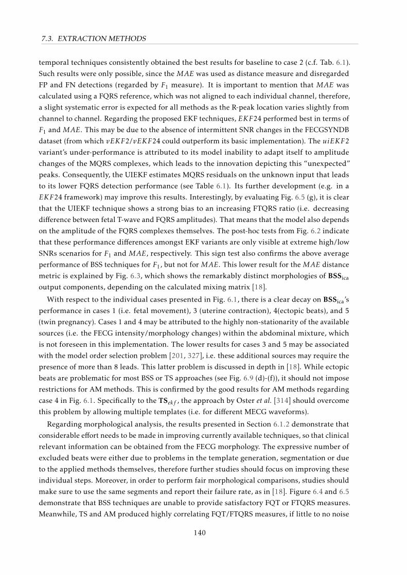
7.3. EXTRACTION METHODS
temporal techniques consistently obtained the best results for baseline to case 2 (c.f. Tab. 6.1).
Such results were only possible, since the MAE was used as distance measure and disregarded
FP and FN detections (regarded by F1 measure). It is important to mention that MAE was
calculated using a FQRS reference, which was not aligned to each individual channel, therefore,
a slight systematic error is expected for all methods as the R-peak location varies slightly from
channel to channel. Regarding the proposed EKF techniques, EKF24 performed best in terms of
F1 and MAE. This may be due to the absence of intermittent SNR changes in the FECGSYNDB
dataset (from which vEKF2/vEKF24 could outperform its basic implementation). The uiEKF2
variant’s under-performance is attributed to its model inability to adapt itself to amplitude
changes of the MQRS complexes, which leads to the innovation depicting this “unexpected”
peaks. Consequently, the UIEKF estimates MQRS residuals on the unknown input that leads
to its lower FQRS detection performance (see Table 6.1). Its further development (e.g. in a
EKF24 framework) may improve this results. Interestingly, by evaluating Fig. 6.5 (g), it is clear
that the UIEKF technique shows a strong bias to an increasing FTQRS ratio (i.e. decreasing
difference between fetal T-wave and FQRS amplitudes). That means that the model also depends
on the amplitude of the FQRS complexes themselves. The post-hoc tests from Fig. 6.2 indicate
that these performance differences amongst EKF variants are only visible at extreme high/low
SNRs scenarios for F1 and MAE, respectively. This sign test also confirms the above average
performance of BSS techniques for F1, but not for MAE. This lower result for the MAE distance
metric is explained by Fig. 6.3, which shows the remarkably distinct morphologies of BSSica
output components, depending on the calculated mixing matrix [18].
With respect to the individual cases presented in Fig. 6.1, there is a clear decay on BSSica’s
performance in cases 1 (i.e. fetal movement), 3 (uterine contraction), 4(ectopic beats), and 5
(twin pregnancy). Cases 1 and 4 may be attributed to the highly non-stationarity of the available
sources (i.e. the FECG intensity/morphology changes) within the abdominal mixture, which
is not foreseen in this implementation. The lower results for cases 3 and 5 may be associated
with the model order selection problem [201, 327], i.e. these additional sources may require the
presence of more than 8 leads. This latter problem is discussed in depth in [18]. While ectopic
beats are problematic for most BSS or TS approaches (see Fig. 6.9 (d)-(f)), it should not impose
restrictions for AM methods. This is confirmed by the good results for AM methods regarding
case 4 in Fig. 6.1. Specifically to the TSekf , the approach by Oster et al. [314] should overcome
this problem by allowing multiple templates (i.e. for different MECG waveforms).
Regarding morphological analysis, the results presented in Section 6.1.2 demonstrate that
considerable effort needs to be made in improving currently available techniques, so that clinical
relevant information can be obtained from the FECG morphology. The expressive number of
excluded beats were either due to problems in the template generation, segmentation or due
to the applied methods themselves, therefore further studies should focus on improving these
individual steps. Moreover, in order to perform fair morphological comparisons, studies should
make sure to use the same segments and report their failure rate, as in [18]. Figure 6.4 and 6.5
demonstrate that BSS techniques are unable to provide satisfactory FQT or FTQRS measures.
Meanwhile, TS and AM produced highly correlating FQT/FTQRS measures, if little to no noise
140
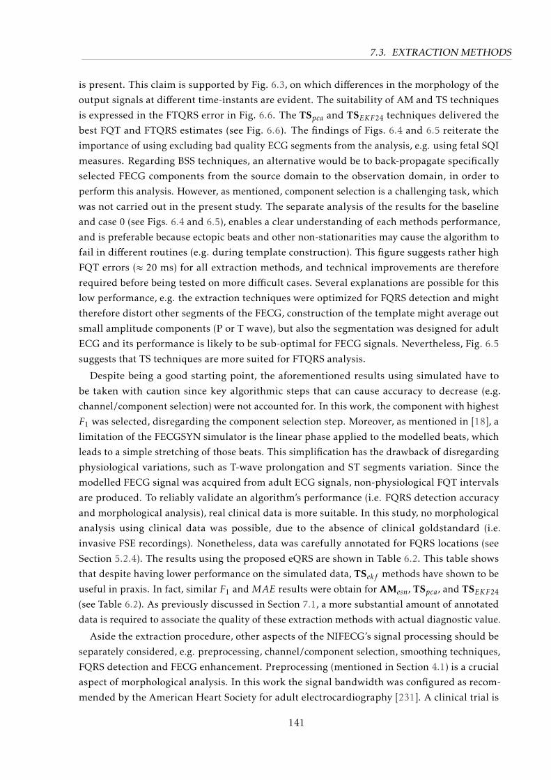
7.3. EXTRACTION METHODS
is present. This claim is supported by Fig. 6.3, on which differences in the morphology of the
output signals at different time-instants are evident. The suitability of AM and TS techniques
is expressed in the FTQRS error in Fig. 6.6. The TSpca and TSEKF24 techniques delivered the
best FQT and FTQRS estimates (see Fig. 6.6). The findings of Figs. 6.4 and 6.5 reiterate the
importance of using excluding bad quality ECG segments from the analysis, e.g. using fetal SQI
measures. Regarding BSS techniques, an alternative would be to back-propagate specifically
selected FECG components from the source domain to the observation domain, in order to
perform this analysis. However, as mentioned, component selection is a challenging task, which
was not carried out in the present study. The separate analysis of the results for the baseline
and case 0 (see Figs. 6.4 and 6.5), enables a clear understanding of each methods performance,
and is preferable because ectopic beats and other non-stationarities may cause the algorithm to
fail in different routines (e.g. during template construction). This figure suggests rather high
FQT errors (≈ 20 ms) for all extraction methods, and technical improvements are therefore
required before being tested on more difficult cases. Several explanations are possible for this
low performance, e.g. the extraction techniques were optimized for FQRS detection and might
therefore distort other segments of the FECG, construction of the template might average out
small amplitude components (P or T wave), but also the segmentation was designed for adult
ECG and its performance is likely to be sub-optimal for FECG signals. Nevertheless, Fig. 6.5
suggests that TS techniques are more suited for FTQRS analysis.
Despite being a good starting point, the aforementioned results using simulated have to
be taken with caution since key algorithmic steps that can cause accuracy to decrease (e.g.
channel/component selection) were not accounted for. In this work, the component with highest
F1 was selected, disregarding the component selection step. Moreover, as mentioned in [18], a
limitation of the FECGSYN simulator is the linear phase applied to the modelled beats, which
leads to a simple stretching of those beats. This simplification has the drawback of disregarding
physiological variations, such as T-wave prolongation and ST segments variation. Since the
modelled FECG signal was acquired from adult ECG signals, non-physiological FQT intervals
are produced. To reliably validate an algorithm’s performance (i.e. FQRS detection accuracy
and morphological analysis), real clinical data is more suitable. In this study, no morphological
analysis using clinical data was possible, due to the absence of clinical goldstandard (i.e.
invasive FSE recordings). Nonetheless, data was carefully annotated for FQRS locations (see
Section 5.2.4). The results using the proposed eQRS are shown in Table 6.2. This table shows
that despite having lower performance on the simulated data, TSekf methods have shown to be
useful in praxis. In fact, similar F1 and MAE results were obtain for AMesn, TSpca, and TSEKF24
(see Table 6.2). As previously discussed in Section 7.1, a more substantial amount of annotated
data is required to associate the quality of these extraction methods with actual diagnostic value.
Aside the extraction procedure, other aspects of the NIFECG’s signal processing should be
separately considered, e.g. preprocessing, channel/component selection, smoothing techniques,
FQRS detection and FECG enhancement. Preprocessing (mentioned in Section 4.1) is a crucial
aspect of morphological analysis. In this work the signal bandwidth was configured as recom-
mended by the American Heart Society for adult electrocardiography [231]. A clinical trial is
141
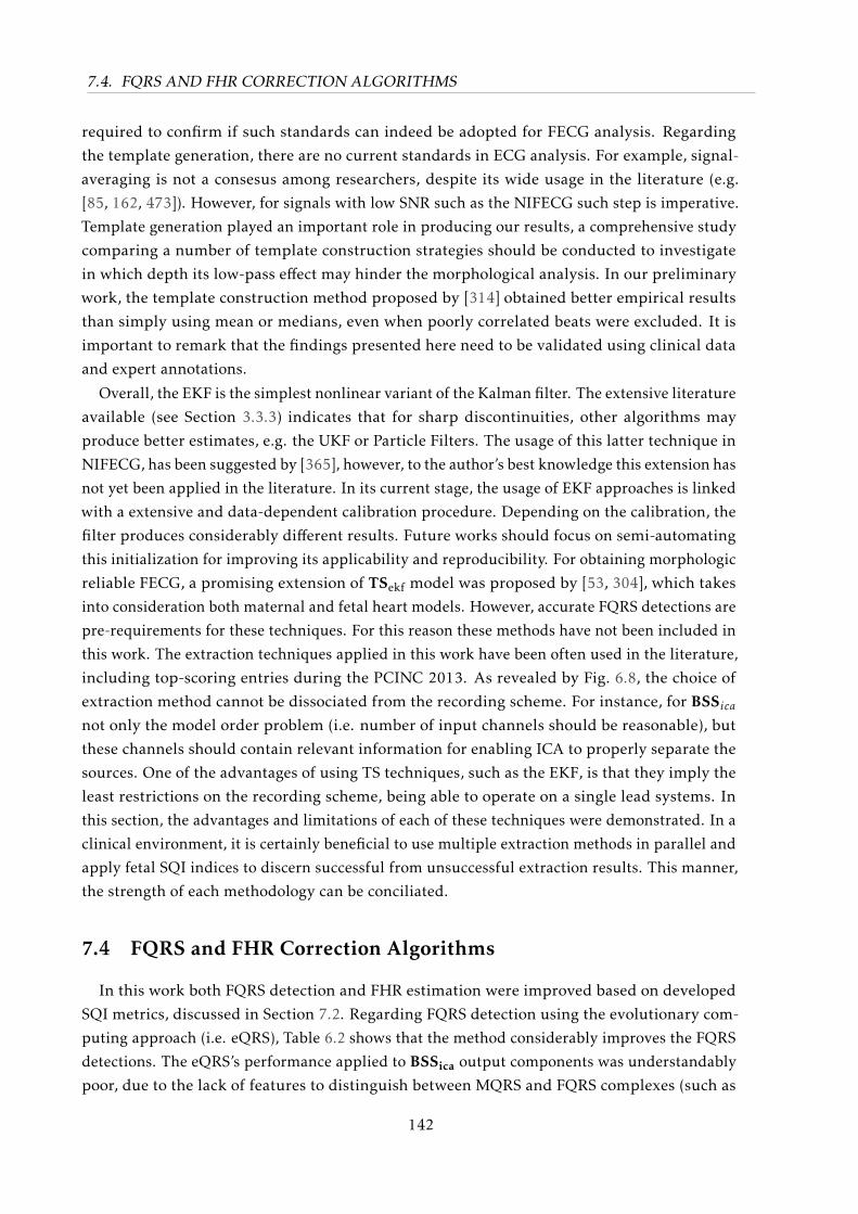
7.4. FQRS AND FHR CORRECTION ALGORITHMS
required to confirm if such standards can indeed be adopted for FECG analysis. Regarding
the template generation, there are no current standards in ECG analysis. For example, signal-
averaging is not a consesus among researchers, despite its wide usage in the literature (e.g.
[85, 162, 473]). However, for signals with low SNR such as the NIFECG such step is imperative.
Template generation played an important role in producing our results, a comprehensive study
comparing a number of template construction strategies should be conducted to investigate
in which depth its low-pass effect may hinder the morphological analysis. In our preliminary
work, the template construction method proposed by [314] obtained better empirical results
than simply using mean or medians, even when poorly correlated beats were excluded. It is
important to remark that the findings presented here need to be validated using clinical data
and expert annotations.
Overall, the EKF is the simplest nonlinear variant of the Kalman filter. The extensive literature
available (see Section 3.3.3) indicates that for sharp discontinuities, other algorithms may
produce better estimates, e.g. the UKF or Particle Filters. The usage of this latter technique in
NIFECG, has been suggested by [365], however, to the author’s best knowledge this extension has
not yet been applied in the literature. In its current stage, the usage of EKF approaches is linked
with a extensive and data-dependent calibration procedure. Depending on the calibration, the
filter produces considerably different results. Future works should focus on semi-automating
this initialization for improving its applicability and reproducibility. For obtaining morphologic
reliable FECG, a promising extension of TSekf model was proposed by [53, 304], which takes
into consideration both maternal and fetal heart models. However, accurate FQRS detections are
pre-requirements for these techniques. For this reason these methods have not been included in
this work. The extraction techniques applied in this work have been often used in the literature,
including top-scoring entries during the PCINC 2013. As revealed by Fig. 6.8, the choice of
extraction method cannot be dissociated from the recording scheme. For instance, for BSSicanot only the model order problem (i.e. number of input channels should be reasonable), but
these channels should contain relevant information for enabling ICA to properly separate the
sources. One of the advantages of using TS techniques, such as the EKF, is that they imply the
least restrictions on the recording scheme, being able to operate on a single lead systems. In
this section, the advantages and limitations of each of these techniques were demonstrated. In a
clinical environment, it is certainly beneficial to use multiple extraction methods in parallel and
apply fetal SQI indices to discern successful from unsuccessful extraction results. This manner,
the strength of each methodology can be conciliated.
7.4 FQRS and FHR Correction Algorithms
In this work both FQRS detection and FHR estimation were improved based on developed
SQI metrics, discussed in Section 7.2. Regarding FQRS detection using the evolutionary com-
puting approach (i.e. eQRS), Table 6.2 shows that the method considerably improves the FQRS
detections. The eQRS’s performance applied to BSSica output components was understandably
poor, due to the lack of features to distinguish between MQRS and FQRS complexes (such as
142
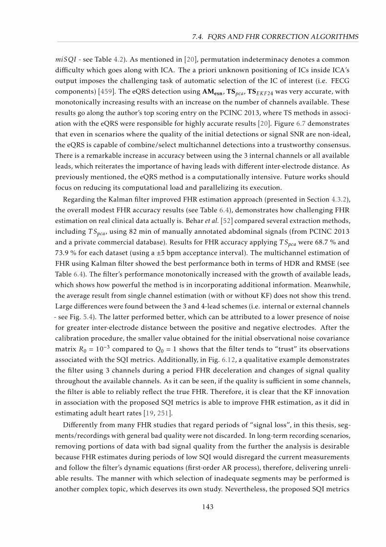
7.4. FQRS AND FHR CORRECTION ALGORITHMS
miSQI - see Table 4.2). As mentioned in [20], permutation indeterminacy denotes a common
difficulty which goes along with ICA. The a priori unknown positioning of ICs inside ICA’s
output imposes the challenging task of automatic selection of the IC of interest (i.e. FECG
components) [459]. The eQRS detection using AMesn, TSpca, TSEKF24 was very accurate, with
monotonically increasing results with an increase on the number of channels available. These
results go along the author’s top scoring entry on the PCINC 2013, where TS methods in associ-
ation with the eQRS were responsible for highly accurate results [20]. Figure 6.7 demonstrates
that even in scenarios where the quality of the initial detections or signal SNR are non-ideal,
the eQRS is capable of combine/select multichannel detections into a trustworthy consensus.
There is a remarkable increase in accuracy between using the 3 internal channels or all available
leads, which reiterates the importance of having leads with different inter-electrode distance. As
previously mentioned, the eQRS method is a computationally intensive. Future works should
focus on reducing its computational load and parallelizing its execution.
Regarding the Kalman filter improved FHR estimation approach (presented in Section 4.3.2),
the overall modest FHR accuracy results (see Table 6.4), demonstrates how challenging FHR
estimation on real clinical data actually is. Behar et al. [52] compared several extraction methods,
including T Spca, using 82 min of manually annotated abdominal signals (from PCINC 2013
and a private commercial database). Results for FHR accuracy applying T Spca were 68.7 % and
73.9 % for each dataset (using a ±5 bpm acceptance interval). The multichannel estimation of
FHR using Kalman filter showed the best performance both in terms of HDR and RMSE (see
Table 6.4). The filter’s performance monotonically increased with the growth of available leads,
which shows how powerful the method is in incorporating additional information. Meanwhile,
the average result from single channel estimation (with or without KF) does not show this trend.
Large differences were found between the 3 and 4-lead schemes (i.e. internal or external channels
- see Fig. 5.4). The latter performed better, which can be attributed to a lower presence of noise
for greater inter-electrode distance between the positive and negative electrodes. After the
calibration procedure, the smaller value obtained for the initial observational noise covariance
matrix R0 = 10−3 compared to Q0 = 1 shows that the filter tends to “trust” its observations
associated with the SQI metrics. Additionally, in Fig. 6.12, a qualitative example demonstrates
the filter using 3 channels during a period FHR deceleration and changes of signal quality
throughout the available channels. As it can be seen, if the quality is sufficient in some channels,
the filter is able to reliably reflect the true FHR. Therefore, it is clear that the KF innovation
in association with the proposed SQI metrics is able to improve FHR estimation, as it did in
estimating adult heart rates [19, 251].
Differently from many FHR studies that regard periods of “signal loss”, in this thesis, seg-
ments/recordings with general bad quality were not discarded. In long-term recording scenarios,
removing portions of data with bad signal quality from the further the analysis is desirable
because FHR estimates during periods of low SQI would disregard the current measurements
and follow the filter’s dynamic equations (first-order AR process), therefore, delivering unreli-
able results. The manner with which selection of inadequate segments may be performed is
another complex topic, which deserves its own study. Nevertheless, the proposed SQI metrics
143
7.4. FQRS AND FHR CORRECTION ALGORITHMS
and classifier are a favorable starting point for further studies. In Section 3.5 a series of HR
preprocessing algorithms were presented that aim at improving such FHR estimates before the
multichannel fusion e.g. with the presented KF approach takes place [19].
In this work, multiple KFs running parallel were implemented for estimating each of individ-
ual channel FHR. The multichannel fusion was considered as an additional step following this
single-channel estimation. Oster and Clifford [315] proposed combining both single-channel
FHR estimation and data fusion steps into a single step, rather than implementing multiple KF
and fusing those later on. This is performed by considering the consensus amongst those differ-
ent sensors as an additional Kalman state and allowing the transition and observational matrices
(Ak and Hk) to be time-variant and dynamically include the previously defined weighting factors
σ2k,s (see Eq. 4.23) [19].
When comparing the accuracy results for the eQRS and KF FHR algorithms (i.e. Table 6.2)
and 6.4), the reader should keep in mind that these algorithms were designed for different
applications. The eQRS is a brute force, offline method with high demand for computational
power. On the other hand, the KF algorithm for FHR is light weight, online and can be ported
to relatively simple hardware structures. Both algorithms were initiated with FQRS detections
provided by simple detectors which correspond to the “Initial” column (in Table 6.2) and “single
channel average (without KF)” row (in Table 6.4). As it can be noticed, these results are indeed
similar for F1 and HDR (regarding TSpca).
In summary, these results reiterate the importance of having SQI metrics, in order to improve
the algorithmic specificity in NIFECG processing. Future works should focus on further devel-
oping those correction algorithms as well as further develop and explore SQI metrics and their
possible combinations of those. Possible SQI enhancements are, e.g. modifications on cSQI to
allow ectopic beats (as preliminary works at the IBMT [472]), or allowing some flexibility on
the FQRS regularity metrics (e.g. rsqi) so that arrhythmic episodes are better described.
144
Barba non facit philosophum
– attributed to Herodes Atticus by Aulus Gellius
8Conclusion
In this work, several relevant aspects regarding the NIFECG research were addressed. For
instance, the lack of publicly available databases containing gold standards for FQRS locations
and FECG morphology was tackled by further developing an elaborate FECGSYN simulator.
This well-defined framework was utilized in creating a large freely available Physionet dataset
comprising simulated abdominal signals that model different non-stationary scenarios and
pathophysiological conditions.
Aside from the produced simulated data, a large private clinical study was carried out in
partnership with the University Hospital of Leipzig. This exploratory study enabled further
insights on the nature of the NIFECG signal (particularly at earlier stages of pregnancy, i.e.
WOG<28). Moreover, the data supplied important information on the recording technique
(e.g. channel selection). Throughout the development of this work, this promising clinical trial
evolved into a multimodal study that shall be continued. Future works on the clinical front
should aim at generating large randomized trial, to conclusively confirm NIFECG’s clinical
relevance in prenatal monitoring.
Regarding signal processing methods for NIFECG, this study focused on pushing forward
open-source algorithms for enabling direct comparison amongst researchers. For this purpose,
the FECGSYN toolbox was furnished with a substantial number of state-of-the-art NIFECG
extraction techniques, statistical performance metrics for FQRS detection and morphological
analysis. To improve the specificity of current methodologies, novel fetal SQI metrics were
proposed, accordingly tested, and included in the FECGSYN toolbox.
A large part of this work dealt with improving the EKF framework. This was performed
by enhancing its model to account for the different signal sources contained in abdECG. For
this purpose, the EKF2 and EKF24 models served as base implementations. In order to cope
with changes of signal quality, a new time-varying method for updating the observational noise
covariance matrix was proposed (i.e. vEKF2 and vEKF24). A common misconception made
145
by current models is the assumption that the FECG can be considered as a white Gaussian
noise. To deal with this model inaccuracy, the unknown input Kalman model is suggested
(uiEKF2). Several experiments were conducted to benchmark the performance of those NIFECG
extraction methods in their capacity to evaluate the FQRS locations, FQT length and FTQRS
ratio. The advantages and limitations of each method were throughly described. Since no
extraction algorithm performs systematically better on every experiment, a combination of
different extraction techniques should be considered for further applications.
Aside from extraction methods and signal quality estimation, this work focused on improving
multichannel FQRS detection and FHR estimation. The first, was performed using a newly
developed evolutionary algorithm for offline correction of FQRS locations. The brute force
search method showed to be highly accurate and is regarded as main responsible for the author’s
top scoring entry on the PCINC 2013 challenge. On the other hand, FHR estimation was
improved by applying the novel developed SQI metrics on a linear Kalman filter for fusing
multichannel information. The algorithm obtained more accurate results than traditional
techniques, additionally, its usage is compatible with online applications.
In summary, this dissertation dealt with several steps of the NIFECG signal processing
chain. Future works should further fine-tune current extraction methods. Moreover, alternative
machine learning approaches to combine the proposed SQI metrics could improve the signal
quality estimation for abdominal signals. At last, NIFECG-specific segmentation algorithms are
required for improving the reliability of FECG’s morphology analysis.
146

References
[1] ADInstruments. Bio Amp Owner ’ s Guide. 2009.
[2] ADInstruments. Powerlab / 30 Series Owner ’ s Guide. 2009.
[3] Afonso, V. X., Tompkins, W. J., Nguyen, T. Q., and Luo, S. ECG Beat Detection Using Filter Banks.IEEE Trans. Biomed. Eng., 46(2):pp. 192–202, 1999.
[4] Agostinelli, A., Grillo, M., Biagini, A., Giuliani, C., Burattini, L., Fioretti, S., Di Nardo, F., Giannu-bilo, S. R., Ciavattini, A., and Burattini, L. Noninvasive Fetal Electrocardiography: An Overview ofthe Signal Electrophysiological Meaning, Recording Procedures, and Processing Techniques. Ann.Noninvasive Electrocardiol., 20(4):pp. 303–313, 2015.
[5] Ahlstrom, M. L. and Tompkins, W. J. Automated High-Speed Analysis of Holter Tapes withMicrocomputers. IEEE Trans. Biomed. Eng., BME-30(10):pp. 651–657, 1983.
[6] Akhbari, M., Shamsollahi, M., Jutten, C., and Coppa, B. ECG Denoising using Angular Velocityas a State and an Observation in an Extended Kalman Filter Framework. In: IEEE EMBC, pp.2897–2900. IEEE, 2012.
[7] Akhbari, M., Shamsollahi, M. B., Jutten, C., Armoundas, A. A., and Sayadi, O. ECG denoising andfiducial point extraction using an extended Kalman filtering framework with linear and nonlinearphase observations. Physiol. Meas., 37(2):pp. 203–226, 2016.
[8] Alfirevic, Z., Devane, D., and Gyte, G. M. Continuous cardiotocography (CTG) as a form ofelectronic fetal monitoring (EFM) for fetal assessment during labour. Cochrane Database Syst. Rev.,5:p. CD006066, 2013.
[9] Almeida, R., Gonçalves, H., Bernardes, J., and Rocha, A. P. Fetal QRS detection and heart rateestimation: a wavelet-based approach. Physiol. Meas., 35(8):pp. 1723–35, 2014.
[10] Alspach, D. and Sorenson, H. Nonlinear Bayesian estimation using Gaussian sum approximations.IEEE Trans. Autom. Control., 17(4):pp. 439–448, 1972.
[11] Amer-Wåhlin, I. and Maršál, K. ST analysis of fetal electrocardiography in labor. Semin. FetalNeonatal Med., 16(1):pp. 29–35, 2011.
[12] American College of Obstetricians and Gynecologists. ACOG Practice Bulletin No. 106: In-trapartum fetal heart rate monitoring: nomenclature, interpretation, and general managementprinciples. Obs. Gynecol, 114(1):pp. 192–202, 2009.
[13] American Heart Association. Congenital Heart Defects in Children Fact Sheet. 2016. URLhttp://www.americanheart.org/children.
[14] Anderson, B. D. O. and Moore, J. B. Optimal Filtering. Prentice Hall, Inc., 2012. ISBN 0-13-638122-7.
[15] Andersson, S. Acceleration and Deceleration Detection and Baseline Estimation. Technical report,Chalmers University of Technology, Götenborg, Sweden, 2011.
[16] Andreotti, F. Extraction of the Fetal ECG from Electrocardiographic Long-term Recordings.Technical report, TU Dresden, Dresden, 2011.
147

REFERENCES
[17] Andreotti, F., Behar, J., Oster, J., Clifford, G. D., Malberg, H., and Zaunseder, S. OptimizedModelling of Maternal ECG Beats Using the Stationary Wavelet Transform. In: Comput. Cardiol.(2010). Cambridge, USA, 2014.
[18] Andreotti, F., Behar, J., Zaunseder, S., Oster, J., and Clifford, G. D. An Open-Source Framework forStress-Testing Non-Invasive Foetal ECG Extraction Algorithms. Physiol. Meas., 37(5):pp. 627–648,2016.
[19] Andreotti, F., Gräßer, F., Malberg, H., and Zaunseder, S. Non-Invasive Fetal ECG Signal QualityAssessment for Multichannel Heart Rate Estimation. IEEE Trans. Biomed. Eng., (in rev.), 2017.
[20] Andreotti, F., Riedl, M., Himmelsbach, T., Wedekind, D., Wessel, N., Stepan, H., Schmieder, C.,Jank, A., Malberg, H., and Zaunseder, S. Robust fetal ECG extraction and detection from abdominalleads. Physiol. Meas., 35(8):pp. 1551–1567, 2014.
[21] Andreotti, F., Riedl, M., Himmelsbach, T., Wedekind, D., Zaunseder, S., Wessel, N., and Malberg,H. Maternal signal estimation by Kalman Filtering and Template Adaptation for fetal heart rateextraction. In: Comput. Cardiol. (2010)., volume 40, pp. 193–196. Zaragoza, Spain, 2013. ISBN9781479908844.
[22] Andreotti, F., Trumpp, A., Malberg, H., and Zaunseder, S. Improved heart rate detection forcamera-based photoplethysmography by means of Kalman filtering. In: IEEE Conf. Electron.Nanotechnol., pp. 428–433. IEEE, Kiev, Ukraine, 2015. ISBN 978-1-4673-6534-5.
[23] Andreotti, F., Zaunseder, S., Schmieder, C., Schröder, S., Löther, S., Malberg, H., Stepan, H., Wessel,N., and Jank, A. Einfluss der mütterlichen EKG-Modellierung auf die fetalen QRS-Detektionen.In: Automed, pp. 12–13. Steinbeis-Edition, Dresden, 2013. ISBN 978-3-943356-82-3.
[24] Andreotti, F., Zaunseder, S., Schmieder, C., Wessel, N., Malberg, H., Stepan, H., and Jank, A.Mehrkanalige Extraktion des fetalen EKGs mittels Kalman-Filter. In: Dresdner Medizintechnik-Symposium, volume 14, pp. 241—-242. TUD Press, Dresden, 2012. ISBN 978-3-942710-96-1.
[25] Annunziata, M. L., Scala, M., Giuliano, N., Tagliaferri, S., Imperato, O. C. M., Esposito, F. G.,Campanile, M., and Di Lieto, A. Fetal vibroacoustic stimulation in computerized cardiotocographicanalysis: The role of short-term variability and approximate entropy. J. Pregnancy, 2012, 2012.
[26] ANSI/ AAMI EC57. Testing and reporting performance results of cardiac rhythm and ST-segmentmeasurement algorithms. Technical Report EC57, American National Standards Institute, Inc. /Association for the Advancement of Medical Instrumentation, 1998.
[27] ANSI/AAMI - EC13:2002. Cardiac monitors, heart rate meters, and alarms. Technical report,American National Standard / Association for the Advancement of Medical Instrumentation(ANSI/AAMI), 2002.
[28] Apgar, V. The newborn (Apgar) scoring system. Reflections and advice. Pediatr. Clin. North Am.,13(3):pp. 645–650, 1966.
[29] Apitz, J., von Brenndorff, C. I., Bruhns, T., and Enders, H. Pädiatrische Kardiologie. Springer Berlin/ Heidelberg, Heidelberg, 1998. ISBN 978-3-642-53755-4.
[30] Armstrong, L. and Stenson, B. J. Use of umbilical cord blood gas analysis in the Assessment of theNewborn. Arch. Dis. Child., pp. 430–434, 2007.
[31] Arnold, M., Miltner, W. H., Witte, H., Bauer, R., and Braun, C. Adaptive AR modeling of nonsta-tionary time series by means of Kalman filtering. IEEE Trans. Biomed. Eng., 45(5):pp. 553–562,1998.
[32] Artal, R., Rutherford, S., Romem, Y., Kammula, R. K., Dorey, F. J., and Wiswell, R. A. Fetal heartrate responses to maternal exercise. Am. J. Obs. Gynecol., 155(4):pp. 729–733, 1986.
148
REFERENCES
[33] Arulampalam, M., Maskell, S., Gordon, N., and Clapp, T. A tutorial on particle filters for onlinenonlinear/non-Gaussian Bayesian tracking. IEEE Trans. Signal Process., 50(2):pp. 174–188, 2002.
[34] Assaleh, K. Extraction of fetal electrocardiogram using adaptive neuro-fuzzy inference systems.IEEE Trans. Biomed. Eng., 2007.
[35] Assaleh, K. and Al-Nashash, H. A novel technique for the extraction of fetal ECG using polynomialnetworks. IEEE Trans. Biomed. Eng., 2005.
[36] AWMF. 015-029 S1: Empfehlungen zum Vorgehen beim vorzeitigen Blasensprung. Technicalreport, Deutsche Gesellschaft für Gynäkologie und Geburtshilfe, 2006.
[37] Ayat, M., Assaleh, K., and Al-Nashash, H. A Novel Methodology for Fetal Heart Rate Extractionfrom the Abdominal Electrocardiogram. In: Int. Biomed. Eng. Conf., pp. 1–5. IEEE, 2008. ISBN9781424426959.
[38] Ayres-de Campos, D. and Arulkumaran, S. FIGO consensus guidelines on intrapartum fetalmonitoring: Physiology of fetal oxygenation and the main goals of intrapartum fetal monitoring.Int. J. Gynaecol. Obs., 131(1):pp. 5–8, 2015.
[39] Ayres-de Campos, D. and Bernardes, J. Twenty-five years after the FIGO guidelines for the use offetal monitoring: time for a simplified approach? Int. J. Gynaecol. Obs., 110(1):pp. 1–6, 2010.
[40] Ayres-de campos, D., Bernardes, J., Garrido, A., Marques-de sá, J., and Pereira-leite, L. SisPorto2.0: A Program for Automated Analysis of Cardiotocograms. J. Matern. Fetal Med., 9:pp. 311–318,2000.
[41] Ayres-de Campos, D., Spong, C. Y., and Chandraharan, E. FIGO consensus guidelines on intra-partum fetal monitoring: Cardiotocography. Int. J. Gynaecol. Obs., 131(1):pp. 13–24, 2015.
[42] Bacharakis, E., Nandi, A., and Zarzoso, V. Foetal ECG extraction using blind source separationmethods. In: EUSIPCO. 1996.
[43] Bäck, T. and Schwefel, H.-P. An overview of evolutionary algorithms for parameter optimization.Evol. Comput., 1(1):pp. 1–23, 1993.
[44] Bailey, R. E. Intrapartum fetal monitoring. Am. Fam. Physician, 80(12):pp. 1388–1396, 2009.
[45] Barnett, S. B., Ter Haar, G. R., Ziskin, M. C., Rott, H. D., Duck, F. A., and Maeda, K. Internationalrecommendations and guidelines for the safe use of diagnostic ultrasound in medicine. UltrasoundMed. Biol., 26(3):pp. 355–366, 2000.
[46] Baumert, M., Porta, A., Vos, M. A., Malik, M., Couderc, J.-P., Laguna, P., Piccirillo, G., Smith,G. L., Tereshchenko, L. G., and Volders, P. G. A. QT interval variability in body surface ECG:measurement, physiological basis, and clinical value: position statement and consensus guidanceendorsed by the European Heart Rhythm Association jointly with the ESC Working Group onCardiac Cellular Electroph. Europace, pp. euv405–, 2016.
[47] Becker, J. H., Krikhaar, A., Schuit, E., Mårtendal, A., Maršál, K., Kwee, A., Visser, G. H. A.,and Amer-Wåhlin, I. The added predictive value of biphasic events in ST analysis of the fetalelectrocardiogram for intrapartum fetal monitoring. Acta Obs. Gynecol. Scand., 94(2):pp. 175–82,2015.
[48] Becker, J. H., Westerhuis, M. E. M. H., Sterrenburg, K., van den Akker, E. S. A., van Beek, E., Bolte,A. C., van Dessel, T. J. H. M., Drogtrop, A. P., van Geijn, H. P., Graziosi, G. C. M., van Lith, J. M. M.,Mol, B. W. J., Moons, K. G. M., Nijhuis, J. G., Oei, S. G., Oosterbaan, H. P., Porath, M. M., Rijnders,R. J. P., Schuitemaker, N. W. E., Wijnberger, L. D. E., Willekes, C., Visser, G. H. A., and Kwee,A. Fetal blood sampling in addition to intrapartum ST-analysis of the fetal electrocardiogram:evaluation of the recommendations in the Dutch STAN® trial. BJOG, 118(10):pp. 1239–1246,2011.
149

REFERENCES
[49] Behar, J. Extraction of Clinical Information from the Non-Invasive Fetal Electrocardiogram. Ph.d.thesis, University of Oxford, 2014.
[50] Behar, J., Andreotti, F., Zaunseder, S., Li, Q., Oster, J., and Clifford, G. D. An ECG Model forSimulating Maternal-Foetal Activity Mixtures on Abdominal ECG Recordings. Physiol. Meas.,35(8):pp. 1537–1550, 2014.
[51] Behar, J., Andreotti, F., Zaunseder, S., Oster, J., and Clifford, G. D. A Practical Guide to Non-Invasive Foetal Electrocardiogram Extraction and Analysis. Physiol. Meas., 37(5):pp. R1–R35,2016.
[52] Behar, J., Johnson, A. E., Clifford, G. D., and Oster, J. A Comparison of Single Channel Fetal ECGExtraction Methods. Ann. Biomed. Eng., 42(6):pp. 1340–1353, 2014.
[53] Behar, J., Oster, J., Andreotti, F., and Clifford, G. D. A Bayesian Filtering Framework for AccurateExtracting of the Non Invasive FECG Morphology. In: Comput. Cardiol. (2010)., pp. 53–56. IEEE,Cambridge, USA, 2014.
[54] Behar, J., Oster, J., and Clifford, G. D. Combining and Benchmarking Methods of Foetal ECGExtraction Without Maternal or Scalp Electrode Data. Physiol. Meas., 35(8):pp. 1569–1589, 2014.
[55] Behar, J., Oster, J., Li, Q., Clifford, G. D., and Member, S. ECG Signal Quality During Arrhythmiaand Its Application to False Alarm Reduction. IEEE Trans. Biomed. Eng., 60(6):pp. 1660–1666,2013.
[56] Behar, J., Zhu, T., Oster, J., Niksch, A., Mah, D., Chun, T., Greenberg, J., Tanner, C., Harrop,J., Esbroeck, A. V., Alexander, A., McCarroll, M., Drake, T., Silber, A., Sameni, R., Ward, J.,Wolfberg, A., and Clifford, G. D. Evaluation of the Fetal QT Interval Using Non-Invasive FetalECG Technology. In: SMFM’s Annu. Pregnancy Meet. 2013.
[57] Belfort, M. A., Saade, G. R., Thom, E., Blackwell, S. C., Reddy, U. M., Thorp, J. M., Tita, A. T., Miller,R. S., Peaceman, A. M., McKenna, D. S., Chien, E. K., Rouse, D. J., and Peter, J. A Randomized Trialof Intrapartum Fetal ECG ST-Segment Analysis. N. Engl. J. Med., 373(7):pp. 632–641, 2015.
[58] Benitez, D. S., Gaydecki, P. a., Zaidi, a., and Fitzpatrick, a. P. A new QRS detection algorithmbased on the Hilbert transform. In: Comput. Cardiol. (2010)., volume 27, pp. 379–382. 2000. ISBN0780365577.
[59] Berger, R. D., Kasper, E. K., Baughman, K. L., Marban, E., Calkins, H., and Tomaselli, G. F. Beat-to-Beat QT Interval Variability : Novel Evidence for Repolarization Lability in Ischemic andNonischemic Dilated Cardiomyopathy. Circulation, 96(5):pp. 1557–1565, 1997.
[60] Bergstra, J. and Bengio, Y. Random search for hyper-parameter optimization. J. Mach. Learn. Res.,13:pp. 281–305, 2012.
[61] Bergveld, P. and Meijer, W. J. A new technique for the suppression of the MECG. IEEE Trans.Biomed. Eng., 28(4):pp. 348–54, 1981.
[62] Bernardes, J., Costa-Pereira, A., Ayres-de Campos, D., Geijn, H., and Pereira-Leite, L. Evaluationof interobserver agreement of cardiotocograms. Int. J. Gynaecol. Obs., 57(1):pp. 33–37, 1997.
[63] Bhide, A., Chandraharan, E., and Acharya, G. Fetal monitoring in labor: Implications of evidencegenerated by new systematic review. Acta Obs. Gynecol. Scand., 95(1):pp. 5–8, 2016.
[64] Billman, G. E. Heart rate variability - a historical perspective. Front. Physiol., 2:p. 86, 2011.
[65] Blackburn, S. Maternal, Fetal, and Neonatal Physiology: A Clinical Perspective. Elsevier Saunders,2014. ISBN 1437716237.
150
REFERENCES
[66] Blix, E., Brurberg, K. G., Reierth, E., Reinar, L. M., and Øian, P. ST waveform analysis vs.cardiotocography alone for intrapartum fetal monitoring: A systematic review and meta-analysisof randomized trials. Acta Obs. Gynecol. Scand., 2015.
[67] Bobrow, C. S. and Soothill, P. W. Causes and consequences of fetal acidosis. Arch. Dis. Child. FetalNeonatal Ed., 80:pp. F246–F249, 1999.
[68] Bousseljot, R., Kreiseler, D., and Schnabel, A. Nutzung der EKG-Signaldatenbank CARDIODATder PTB über das Internet. Biomed. Tech., 40(s1):pp. 317–318, 1995.
[69] Brodsky, D. and Christou, H. Current concepts in intrauterine growth restriction. J. Intensive CareMed., 19(6):pp. 307–19, 2004.
[70] Brown, R. G. and Hwang, P. Y. C. Introduction to Random Signals and Applied Kalman Filtering withMatlab Exercises. John Wiley & Sons, 1983. ISBN 0470609699.
[71] Bucy, R. and Joseph, P. Filtering for stochastic processes with applications to guidance. John Wiley &Sons, 1968. ISBN 470 116528.
[72] Bundesamt für Statistik. Neugeborene in Schweizer Spitälern 2004 : Spitalversorgung von termin-und frühgeborenen Säuglingen. Technical report, Bundesamt für Statistik (BFS) - Swiss Federation,2007.
[73] Bundesinstitut für Bevölkerungsforschung. Perinatalsterblichkeit. 2016. URL http://www.
bib-demografie.de/DE/Institut/Jahresberichte/jahresberichte_node.html.
[74] Burgers, G., Jan van Leeuwen, P., and Evensen, G. Analysis Scheme in the Ensemble Kalman Filter.Mon. Weather Rev., 126(6):pp. 1719–1724, 1998.
[75] Callaerts, D., De Moor, B., Vandewalle, J., Sansen, W., Vantrappen, G., Janssens, J., Moor, B. D.,Vandewalle, J., Sansen, W., Vantrappen, G., and Janssens, J. Comparison of SVD methods to extractthe foetal electrocardiogram from cutaneous electrode signals. Med. Biol. Eng. Comput., 28(3):pp.217–224, 1990.
[76] Camps, G., Martinez, M., and Soria, E. Fetal ECG extraction using an FIR neural network. In:Comput. Cardiol. (2010)., pp. 249–252. IEEE, 2001. ISBN 0-7803-7266-2.
[77] Caughey, A. B., Robinson, J. N., and Norwitz, E. R. Contemporary diagnosis and management ofpreterm premature rupture of membranes. Rev. Obstet. Gynecol., 1(1):pp. 11–22, 2008.
[78] Cerutti, S., Baselli, G., Civardi, S., Ferrazzi, E., Marconi, A. M., Pagani, M., and Pardi, G. Variabilityanalysis of fetal heart rate signals as obtained from abdominal electrocardiographic recordings. J.Perinat. Med., 14(6):pp. 445–452, 1986.
[79] Cerutti, S., Civardi, S., Bianchi, A., Signorini, M. G., Ferrazzi, E., and Pardi, G. Spectral analysis ofantepartum heart rate variability. Clin. Phys. Physiol. Meas., 10(4B):pp. 27–31, 1989.
[80] Chandraharan, E. Authors’ reply: Fetal scalp blood sampling during labour: Is it a useful diagnostictest or a historical test that no longer has a place in modern clinical obstetrics? BJOG, 121(13):pp.1753–1754, 2014.
[81] Chauhan, S. P., Gupta, L. M., Hendrix, N. W., and Berghella, V. Intrauterine growth restriction:comparison of American College of Obstetricians and Gynecologists practice bulletin with othernational guidelines. Am. J. Obs. Gynecol., 200(4):pp. 409.e1–409.e6, 2009.
[82] Chen, Z. Bayesian filtering: From Kalman filters to particle filters, and beyond. Statistics (Ber).,182(1):pp. 1–69, 2003.
[83] Chen, Z. and Chan, L. New approaches for solving permutation indeterminacy and scalingambiguity in frequency domain separation of convolved mixtures. In: Neural Networks (IJCNN),2011 Int. Jt. Conf., pp. 911–918. 2011.
151

REFERENCES
[84] Chung, D. Y., Sim, Y. B., Park, K. T., Yi, S. H., Shin, J. C., and Kim, S. P. Spectral analysis of fetalheart rate variability as a predictor of intrapartum fetal distress. Int. J. Gynaecol. Obs., 73(2):pp.109–16, 2001.
[85] Clifford, G., Sameni, R., Ward, J., Robinson, J., and Wolfberg, A. J. Clinically accurate fetal ECGparameters acquired from maternal abdominal sensors. Am. J. Obs. Gynecol., 205(1):p. 47, 2011.
[86] Clifford, G. D. Signal Processing Methods for Heart Rate Variability. Ph.D. thesis, University ofOxford, 2002.
[87] Clifford, G. D. A novel framework for signal representation and source separation: Applicationsto filtering and segmentation of biosignals. J.Biol. Syst., 14(02):pp. 169–183, 2006.
[88] Clifford, G. D., Azuaje, F., and McSharry, P. E. Advanced methods and tools for ECG data analysis.Artech House, 2006. ISBN 1580539661.
[89] Clifford, G. D., Behar, J., Li, Q., and Rezek, I. Signal quality indices and data fusion for determiningclinical acceptability of electrocardiograms. Physiol. Meas., 33(9):pp. 1419–1433, 2012.
[90] Clifford, G. D. and McSharry, P. E. Method to filter ECGs and evaluate clinical parameter distortionusing realistic ECG model parameter fitting. Comput. Cardiol., 32:pp. 715–718, 2005.
[91] Clifford, G. D., Shoeb, A., McSharry, P. E., and Janz, B. A. Model-based filtering, compression andclassification of the ECG. In: Proc. Bioelectromagn. 5th Int. Symp. Noninvasive Funct. Source Imagingwithin Hum. Brain Hear. (BEM NFSI), pp. 158–161. Minnesota, USA, 2005.
[92] Clifford, G. D., Silva, I., Behar, J., and Moody, G. B. Non-invasive fetal ECG analysis. Physiol. Meas.,35(8):p. 1521, 2014.
[93] Clifford, G. D. and Tarassenko, L. Quantifying errors in spectral estimates of HRV due to beatreplacement and resampling. IEEE Trans. Biomed. Eng., 52(4):pp. 630–8, 2005.
[94] Cohen, J. A coefficient of agreement for nominal scales. Educ. Psychol. Meas., XX(1):pp. 37–46,1960.
[95] Cohen, J. Weighted kappa: Nominal scale agreement provision for scaled disagreement or partialcredit. Psychol. Bull., 1968.
[96] Cohen, J. Statistical Power Analysis for the Behavioral Sciences. L. Erlbaum Associates, 1988. ISBN0805802835.
[97] Cohen, J. A power primer. Psychol. Bull., 112(1):pp. 155–159, 1992.
[98] Couderc, J. P. The Telemetric and Holter ECG Warehouse initiative (THEW): A data repositoryfor the design, implementation and validation of ECG-related technologies. In: IEEE EMBC, pp.6252–6255. 2010. ISBN 9781424441235.
[99] Cremer, M. Über die Direkte Ableitung der Aktionstrome des Menschlichen Herzens vom Oesoph-agus und Über das Elektrokardiogramm des Fetus. Münchener Medizinische Wochenschrift, 53:pp.811–813, 1906.
[100] Crowe, J. a., Harrison, A., and Hayes-Gill, B. R. The feasibility of long-term fetal heart ratemonitoring in the home environment using maternal abdominal electrodes. Physiol. Meas., 16(3):pp.195–202, 1995.
[101] Daluwatte, C., Johannesen, L., Galeotti, L., Vicente, J., Strauss, D. G., and Scully, C. G. AssessingECG signal quality indices to discriminate ECGs with artefacts from pathologically differentarrhythmic ECGs. Physiol. Meas., 37(8):pp. 1370–1382, 2016.
[102] Darouach, M., Zasadzinski, M., and Boutayeb, M. Extension of minimum variance estimation forsystems with unknown inputs. Automatica, 39:pp. 867–876, 2003.
152
REFERENCES
[103] Darouach, M., Zasadzinski, M., Onana, a. B., and Nowakowski, S. Kalman filtering with unknowninputs via optimal state estimation of singular systems. Int. J. Syst. Sci., 26(1995):pp. 2015–2028,1995.
[104] Darwin, C. On the Origin of Species by means of Sexual Selection. D. Appleton and Company, NewYork, N.Y., 1859.
[105] Dawes, G., Rosevear, S., Pello, L., Moulden, M., and Redman, C. Computerized analysis of episodicchanges in fetal heart rate variation in early labor. Am. J. Obs. Gynecol., 165(3):pp. 618–624, 1991.
[106] Dawes, G. S., Houghton, C. R., Redman, C. W., and Visser, G. H. Pattern of the normal humanfetal heart rate. BJOG, 89(4):pp. 276–84, 1982.
[107] Dawes, G. S., Visser, G. H., Goodman, J. D., and Redman, C. W. Numerical analysis of the humanfetal heart rate: the quality of ultrasound records. Am. J. Obs. Gynecol., 141(1):pp. 43–52, 1981.
[108] de Haan, G. and Jeanne, V. Robust pulse-rate from chrominance-based rPPG. IEEE Trans. Biomed.Eng., 60(10):pp. 1–9, 2013.
[109] De Lathauwer, L., De Moor, B., Vandewalle, J., and Lathauwer, L. Fetal electrocardiogramextraction by blind source subspace separation. IEEE Trans. Biomed. Eng., 47(5):pp. 567–572, 2000.
[110] de Vaus, D. Surveys in Social Research. Routledge, 2013. ISBN 1136996311.
[111] Deng, Y., Wolf, W., Schnell, R., and Appel, U. New aspects to event-synchronous cancellationof ECG interference: an application of the method in diaphragmatic EMG signals. IEEE Trans.Biomed. Eng., 47(9):pp. 1177–1184, 2000.
[112] Deutsche Hygiene-Museum Dresden. Mütterliche Fetale Blutkreislauf. 2008.
[113] Di Marco, L., Marzo, A., and Frangi, A. Multichannel Foetal Heartbeat Detection by CombiningSource Cancellation with Expectation-weighted Estimation of Fiducial Points. In: Comput. Cardiol.(2010)., pp. 329–332. 2013.
[114] Dildy, G., Clark, S., and Loucks, C. Preliminary experience with intrapartum fetal pulse oximetryin humans. Obs. Gynecol., 1993.
[115] DiPietro, J. A., Costigan, K. A., and Gurewitsch, E. D. Fetal response to induced maternal stress.Early Hum. Dev., 74(2):pp. 125–138, 2003.
[116] DiPietro, J. A., Costigan, K. A., Nelson, P., Gurewitsch, E. D., and Laudenslager, L. Fetal responsesto induced maternal relaxation during pregnancy. Biol. Psychol., 77(1):pp. 11–19, 2008.
[117] DiPietro, J. a., Hilton, S. C., Hawkins, M., Costigan, K. a., and Pressman, E. K. Maternal stress andaffect influence fetal neurobehavioral development. Dev. Psychobiol., 38(5):pp. 659–668, 2002.
[118] Domingos, P. and Pazzani, M. On the Optimality of the Simple Bayesian Classifier under Zero-OneLos. Mach. Learn., 29(2/3):pp. 103–130, 1997.
[119] DuBose, T. J. Embryonic Heart Rate and Age. J. Diagnostic Med. Sonogr., 6(3):pp. 151–157, 1990.
[120] Duck, F. A. Safety Aspects of the Use of Ultrasound in Pregnancy. Fetal Matern. Med. Rev., 14(1):p.S0965539502001006, 2003.
[121] Durrant-Whyte, H. Introduction to estimation and the Kalman Filter. Technical report, Universityof Sidney, 2001.
[122] East, C. E., Begg, L., Colditz, P. B., and Lau, R. Fetal pulse oximetry for fetal assessment in labour.Cochrane Database Syst. Rev., 10:p. CD004075, 2014.
[123] Ebenezer, D. and Krishnamurthy, V. Wave digital matched filter for electrocardiogram preprocess-ing. J. Biomed. Eng., 15(2):pp. 132–4, 1993.
153

REFERENCES
[124] Escofier, B. Traitement simultané de variables qualitatives et quantitatives en analyse factorielle.Cah. Anal. Donnees, 1979.
[125] Evensen, G. Sequential data assimilation with a nonlinear quasi-geostrophic model using MonteCarlo methods to forecast error statistics. J. Geophys. Res., 99(C5):p. 10143, 1994.
[126] Evensen, G. The ensemble Kalman filter: Theoretical formulation and practical implementation.Ocean Dyn., 53(4):pp. 343–367, 2003.
[127] Evensen, G. Sampling strategies and square root analysis schemes for the EnKF. Ocean Dyn.,54(6):pp. 539–560, 2004.
[128] Evensen, G. Data Assimilation: The Ensemble Kalman Filter. Springer Berlin / Heidelberg, 2007.ISBN 9783540383000.
[129] Fanelli, A. TeleFetal Care: development of a wearable system for fetal monitoring during pregnancy.Ph.D. thesis, Politecnico di Milano, 2013.
[130] Fang, H., de Callafon, R. A., and Cortés, J. Simultaneous input and state estimation for nonlinearsystems with applications to flow field estimation. Automatica, 49(9):pp. 2805–2812, 2013.
[131] Fang, H., Shi, Y., and Yi, J. On stable simultaneous input and state estimation for discrete-timelinear systems. Int. J. Adapt. Control Signal Process., 25(8):pp. 671–686, 2011.
[132] Farrell, T. G., Bashir, Y., Cripps, T., Malik, M., Poloniecki, J., Bennett, E., Ward, D. E., and Camm, A.Risk stratification for arrhythmic events in postinfarction patients based on heart rate variability,ambulatory electrocardiographic variables and the signal-averaged electrocardiogram. J. Am. Coll.Cardiol., 18(3):pp. 687–697, 1991.
[133] Feinstein, A. R. and Cicchetti, D. V. High agreement but low kappa: I. The problems of twoparadoxes. J. Clin. Epidemiol., 43(6):pp. 543–9, 1990.
[134] Ferrario, M., Magenes, G., Campanile, M., Carbone, I. F., Di Lieto, A., and Signorini, M. G.Multiparameter analysis of heart rate variability signal for the investigation of high risk fetuses.In: IEEE EMBC, pp. 4662–4665. 2009.
[135] Ferrario, M., Signorini, M. G., and Magenes, G. Comparison between fetal heart rate standardparameters and complexity indexes for the identification of severe intrauterine growth restriction.Methods Inf. Med., 46(2):pp. 295–298, 2007.
[136] Ferrario, M., Signorini, M. G., and Magenes, G. Estimation of long-term correlations from FetalHeart Rate variability signal for the identification of pathological fetuses. In: IEEE EMBC. 2007.
[137] Ferrario, M., Signorini, M. G., Magenes, G., and Cerutti, S. Comparison of entropy-based regularityestimators: application to the fetal heart rate signal for the identification of fetal distress. IEEETrans. Biomed. Eng., 53(1):pp. 119–125, 2006.
[138] Fleiss, J. Measuring nominal scale agreement among many raters. Psychol. Bull., 1971.
[139] Frank, B., Pompe, B., Schneider, U., and Hoyer, D. Permutation entropy improves fetal behaviouralstate classification based on heart rate analysis from biomagnetic recordings in near term fetuses.Med. Biol. Eng. Comput., 44(3):pp. 179–87, 2006.
[140] Frasch, M. G., Müller, T., Weiss, C., Schwab, K., Schubert, H., and Schwab, M. Heart rate variabilityanalysis allows early asphyxia detection in ovine fetus. Reprod Sci., 16(5):pp. 509–517, 2009.
[141] Frasch, M. G., Xu, Y., Stampalija, T., Durosier, L. D., Herry, C., Wang, X., Casati, D., Seely, A. J.,Alfirevic, Z., Gao, X., and Ferrazzi, E. Correlating multidimensional fetal heart rate variabilityanalysis with acid-base balance at birth. Physiol. Meas., 35(12):pp. L1–12, 2014.
154

REFERENCES
[142] Frei, M. and Kunsch, H. R. Bridging the ensemble Kalman and particle filters. Biometrika, 100(4):pp.781–800, 2013.
[143] Fretts, R. C., Schmittdiel, J., McLean, F. H., Usher, R. H., and Goldman, M. B. Increased maternalage and the risk of fetal death. N. Engl. J. Med., 333(15):pp. 953–957, 1995.
[144] Friesen, G. M., Jannett, T. C., Jadallah, M. A., Yates, S. L., Quint, S. R., and Nagle, H. T. Acomparison of the noise sensitivity of nine QRS detection algorithms. IEEE Trans. Biomed. Eng.,37(1):pp. 85–98, 1990.
[145] Fuchs, T., Pomorski, M., Grobelak, K., Tomiałowicz, M., and Zimmer, M. Signal loss during fetalheart rate monitoring using maternal abdominal surface electrodes between 28 and 42 weeks ofpregnancy. Adv. Clin. Exp. Med., 23(5):pp. 813–9, 2014.
[146] Fukushima, A., Nakai, K., Itoh, M., Horigome, H., Suwabe, A., Tohyama, K., Kobayashi, K.,Yoshizawa, M., and Sugiyama, T. Assessment of Fetal Autonomic Nervous System Activity by FetalMagnetocardiography - ProQuest. Clin. Med. Cardiol., 1:p. 33, 2008.
[147] Funk, N. A Study of the Kalman Filter applied to Visual Tracking. Technical Report 1, Universityof Alberta, 2003.
[148] Gacek, A. and Pedrycz, W. ECG Signal Processing, Classification and Interpretation: A Comprehen-sive Framework of Computational Intelligence. Springer Science & Business Media, 2011. ISBN0857298682.
[149] Gambarotta, N., Aletti, F., Baselli, G., and Ferrario, M. A review of methods for the signal qualityassessment to improve reliability of heart rate and blood pressures derived parameters. Med. Biol.Eng. Comput., 54(7):pp. 1025–35, 2016.
[150] Gardiner, C. W. Handbook of stochastic methods. Springer, 1985. ISBN 3540616349.
[151] Gelb, A. Applied Optimal Estimation. MIT Press, 1974. ISBN 0262570483.
[152] Gennat, M. Extraktion der fetalen Herzrate unter Berücksichtigung der Signalqualität. Technicalreport, Technische Universität Dresden, 2016.
[153] Gerstner, T., Sprenger, J., Schaible, T., Weiss, C., and Koenig, S. Reifung des Autonomen Nerven-systems: Unterschiede in der Herzfrequenzvariabilität in unterschiedlichen Gestationswochen. Z.Geburtshilfe Neonatol., 214(01):pp. 11–14, 2009.
[154] Ghaffari, A., Golbayani, H., and Ghasemi, M. A new mathematical based QRS detector usingcontinuous wavelet transform. Comput. Electr. Eng., 34(2):pp. 81–91, 2008.
[155] Ghaffari, A., Mollakazemi, M. J., Atyabi, S. A., and Niknazar, M. Robust fetal QRS detectionfrom noninvasive abdominal electrocardiogram based on channel selection and simultaneousmultichannel processing. Australas. Phys. Eng. Sci. Med., 2015.
[156] Ghahremani, E. and Kamwa, I. Dynamic state estimation in power system by applying theextended kalman filter with unknown inputs to phasor measurements. IEEE Trans. Power Syst.,26(4):pp. 2556–2566, 2011.
[157] Gierałtowski, J., Hoyer, D., Tetschke, F., Nowack, S., Schneider, U., and Zebrowski, J. Developmentof multiscale complexity and multifractality of fetal heart rate variability. Auton. Neurosci., 178(1-2):pp. 29–36, 2013.
[158] Gillijns, S. and De Moor, B. Unbiased minimum-variance input and state estimation for lineardiscrete-time systems. Automatica, 43(1):pp. 111–116, 2007.
[159] Gillijns, S., Mendoza, O., Chandrasekar, J., De Moor, B., Bernstein, D., and Ridley, A. What is theensemble Kalman filter and how well does it work? In: Am. Control Conf., p. 6 pp. 2006. ISBN1-4244-0209-3.
155

REFERENCES
[160] Gillijns, S. and Moor, B. D. Unbiased minimum-variance input and state estimation for lineardiscrete-time systems with direct feedthrough. Automatica, 2007.
[161] Goldberger, A. L., Amaral, L. A., Glass, L., Hausdorff, J. M., Ivanov, P. C., Mark, R. G., Mietus,J. E., Moody, G. B., Peng, C. K., and Stanley, H. E. PhysioBank, PhysioToolkit, and PhysioNet:components of a new research resource for complex physiologic signals. Circulation, 101(23):pp.E215—-E220, 2000.
[162] Gomes, J. A., Cain, M. E., Buxton, A. E. A., Josephson, M. E., Lee, K. L., and Hafley, G. E. Predictionof Long-Term Outcomes by Signal-Averaged Electrocardiography in Patients With UnsustainedVentricular Tachycardia, Coronary Artery Disease, and Left Ventricular Dysfunction. Circulation,104(4):pp. 436–441, 2001.
[163] Graatsma, E. M., Jacod, B. C., van Egmond, L. A. J., Mulder, E. J. H., and Visser, G. H. A. Fetalelectrocardiography: feasibility of long-term fetal heart rate recordings. BJOG, 116(2):pp. 334—-7,discussion 337–8, 2009.
[164] Graczyk, S., Jezewski, J., Wrobel, J., and Gacek, A. Abdominal electrohysterogram data acquisitionproblems and their source of origin. In: Proc. First Reg. Conf. IEEE Eng. Med. Biol. Soc. 14th Conf.Biomed. Eng. Soc. India. An Int. Meet, pp. PS13–PS14. IEEE, 1995. ISBN 0-7803-2711-X.
[165] Greene, K. R., Dawes, G. S., Lilja, H., and Rosén, K. G. Changes in the ST waveform of the fetallamb electrocardiogram with hypoxemia. Am. J. Obs. Gynecol., 144(8):pp. 950–8, 1982.
[166] Grewal, M. S., Andrews, A. P., and Grewal Mohinder S. l, A. P. A. Kalman filtering: Theory andPractice using Matlab. John Wiley & Sons, Inc., 3rd edition, 2008.
[167] Grunitz, E. Entwicklung von Methoden zur Analyse und Aufbereitung biomedizinischer Mess-daten. Technical report, Technische Universität Dresden, 2012.
[168] Gwet, K. Handbook of inter-rater reliability: The definitive guide to measuring the extent of agreementamong raters. Advanced Analytics, LLC, 2014.
[169] Haghpanahi, M. and Borkholder, D. A. Fetal QRS extraction from abdominal recordings viamodel-based signal processing and intelligent signal merging. Physiol. Meas., 35(8):pp. 1591–605,2014.
[170] Haghpanahi, M., Sameni, R., and Borkholder, D. A. Scoring consensus of multiple ECG annotatorsby optimal sequence alignment. In: IEEE EMBC, volume 2014, pp. 1855–9. 2014.
[171] Hamilton, P. and Tompkins, W. Quantitative investigation of QRS detection rules using theMIT/BIH arrhythmia database. IEEE Trans. Biomed. Eng., 1986.
[172] Harding, R. Fetal pulmonary development: the role of respiratory movements. Equine Vet. J. Suppl.,24:pp. 32–39, 1997.
[173] Hasan, M. a., Reaz, M. B. I., Ibrahimy, M. I., Hussain, M. S., and Uddin, J. Detection and ProcessingTechniques of FECG Signal for Fetal Monitoring. Biol. Proced. Online, 11(1):pp. 263–95, 2009.
[174] Hayes, A. F. and Krippendorff, K. Answering the Call for a Standard Reliability Measure forCoding Data. Commun. Methods Meas., 1(1):pp. 77–89, 2007.
[175] Haykin, S. Kalman Filtering and Neural Networks. Wiley-Interscience, 2001. ISBN 0471369985.
[176] Hernando, D., Bailon, R., Almeida, R., and Hernandez, A. Computing in Cardiology Conference(CinC), 2014. In: Comput. Cardiol. (2010)., pp. 737–740. 2014.
[177] Herrmann, P. Aufnahme und Verarbeitung des kapazitiven Elektrokardiogramms. Diplomarbeit,TU Dresden, 2014.
[178] Hills, M. Embriology. 2016. URL https://embryology.med.unsw.edu.au/embryology/.
156

REFERENCES
[179] Himmelsbach, T. Weiterentwicklung eines Kalman-basierten Algorithmus zur Extraktion desfetalen EKG aus abdominalen Aufnahmen. Technical report, TU Dresden, 2013.
[180] Hoffmann, J. Extraktion von fetalen Elektrokardiogrammen mittels eines zeitvarianten Kalman-Filter Modells. Technical report, Technische Universität Dresden, 2016.
[181] Højgaard, M. V., Holstein-Rathlou, N. H., Agner, E., and Kanters, J. K. Dynamics of spectralcomponents of heart rate variability during changes in autonomic balance. Am. J. Physiol., 275(1Pt 2):pp. H213–9, 1998.
[182] Holschneider, M. and Kronland-Martinet, R. A real-time algorithm for signal analysis with thehelp of the wavelet transform. Wavelets, 1989.
[183] Hon, E. H. and Hess, O. W. Instrumentation of Fetal Electrocardiography. Science (80-. ).,125(3247):pp. 553–554, 1957.
[184] Hon, E. H. and Lee, S. T. Electronic evaluation of the fetal heart rate, VIII. Patterns preceding fetaldeath: Further observations. Am. J. Obs. Gynecol., 87:pp. 814–26, 1963.
[185] Hopkins, P., Outram, N., Löfgren, N., Ifeachor, E. C., and Rosén, K. G. A comparative study offetal heart rate variability analysis techniques. In: IEEE EMBC, volume 1, pp. 1784–7. 2006.
[186] Hou, M. and Patton, R. Optimal filtering for systems with unknown inputs. IEEE Trans. Autom.Contr., 43(3):pp. 445–449, 1998.
[187] Houtekamer, P. and Mitchell, H. L. Ensemble Kalman filtering. Q. J. R. Meteorol. Soc., 131(613):pp.3269–3289, 2005.
[188] Hoyer, D., Heinicke, E., Jaekel, S., Tetschke, F., Di Pietro Paolo, D., Haueisen, J., Schleusner, E.,and Schneider, U. Indices of fetal development derived from heart rate patterns. Early Hum. Dev.,85(6):pp. 379–86, 2009.
[189] Hoyer, D., Nowack, S., Bauer, S., Tetschke, F., Rudolph, A., Wallwitz, U., Jaenicke, F., Heinicke,E., Götz, T., Huonker, R., Witte, O. W., Schleussner, E., and Schneider, U. Fetal development ofcomplex autonomic control evaluated from multiscale heart rate patterns. Am. J. Physiol. Regul.Integr. Comp. Physiol., 304(5):pp. R383–92, 2013.
[190] Hoyer, D., Tetschke, F., Jaekel, S., Nowack, S., Witte, O. W., Schleußner, E., and Schneider, U.Fetal functional brain age assessed from universal developmental indices obtained from neuro-vegetative activity patterns. PLoS One, 8(9):p. e74431, 2013.
[191] Hsieh, C.-S. Robust two-stage Kalman filters for systems with unknown inputs. IEEE Trans. Autom.Contr., 45(12):pp. 2374–2378, 2000.
[192] Hsieh, C.-S. Extension of unbiased minimum-variance input and state estimation for systems withunknown inputs. Automatica, 45(9):pp. 2149–2153, 2009.
[193] Hu, X., Nenov, V., Bergsneider, M., Glenn, T. C., Vespa, P., and Martin, N. Estimation of HiddenState Variables of the Intracranial System Using Constrained Nonlinear Kalman Filters. IEEE Trans.Biomed. Eng., 54(4):pp. 597–610, 2007.
[194] Huelsbusch, M. and Blazek, V. Contactless mapping of rhythmical phenomena in tissue perfu-sion using PPGI. In: Clough, A. V. and Chen, C.-T. (editors), Med. Imaging 2002, pp. 110–117.International Society for Optics and Photonics, San Diego, USA, 2002.
[195] Hurezeanu, B., Ungureanu, G. M., Taralunga, D. D., Strungaru, R., Gussi, I., and Wolf, W. FECGdelineation from abdominal signals using wavelet transform. In: Int. Conf. Expo. Electr. Power Eng.,pp. 518–521. IEEE, 2014. ISBN 978-1-4799-5849-8.
[196] Hutter, D., Kingdom, J., and Jaeggi, E. Causes and mechanisms of intrauterine hypoxia and itsimpact on the fetal cardiovascular system: a review. Int. J. Pediatr., 2010:p. 401323, 2010.
157

REFERENCES
[197] Hyvärinen, A. Fast and robust fixed-point algorithms for independent component analysis. IEEETrans. Neural Netw., 10(3):pp. 626–34, 1999.
[198] Inanlou, M. R., Baguma-Nibasheka, M., and Kablar, B. The role of fetal breathing-like movementsin lung organogenesis. Histol. Histopathol., 20(4):pp. 1261–1266, 2005.
[199] Ivanov, P. C., Ma, Q. D. Y., and Bartsch, R. P. Maternal-fetal heartbeat phase synchronization. Proc.Natl. Acad. Sci. U. S. A., 106(33):pp. 13641–2, 2009.
[200] Jaeger, H. The "echo state" approach to analysing and training recurrent neural networks. Technicalreport, German National Research Center for Information Technology, 2001.
[201] James, C. and Hesse, C. Independent component analysis for biomedical signals. Physiol. Meas.,2005.
[202] James, T. N. Cardiac conduction system: Fetal and postnatal development. Am. J. Cardiol., 25(2):pp.213–226, 1970.
[203] Jane, R., Blasi, A., Garcia, J., and Laguna, P. Evaluation of an automatic threshold based detector ofwaveform limits in Holter ECG with the QT database. In: Comput. Cardiol. (2010)., pp. 295–298.IEEE, 1997. ISBN 0-7803-4445-6.
[204] Jansen, B. H., Bourne, J. R., and Ward, J. W. Autoregressive estimation of short segment spectra forcomputerized EEG analysis. IEEE Trans. Biomed. Eng., 28(9):pp. 630–8, 1981.
[205] Javadi, M., Ebrahimpour, R., Sajedin, A., Faridi, S., and Zakernejad, S. Improving ECG classificationaccuracy using an ensemble of neural network modules. PLoS One, 6(10):p. e24386, 2011.
[206] Jazwinski, A. H. Stochastic Processes and Filtering Theory. Courier Corporation, 1970. ISBN0080960901.
[207] Jérôme, P. Analyse factorielle de données mixtes. Rev. Stat. appliquée, 52(4):pp. 93—-111, 2002.
[208] Jezewski, J., Matonia, A., Kupka, T., Roj, D., and Czabanski, R. Determination of fetal heartrate from abdominal signals: evaluation of beat-to-beat accuracy in relation to the direct fetalelectrocardiogram. Biomed. Tech., 57(5):pp. 383–94, 2012.
[209] Johnson, A. E. W., Behar, J., Andreotti, F., Clifford, G. D., and Oster, J. R-Peak Estimation usingMultimodal Lead Switching. In: Comput. Cardiol. (2010)., pp. 281–284. IEEE, Cambridge, USA,2014.
[210] Johnson, A. E. W., Cholleti, S. R., Buchman, T. G., and Clifford, G. D. Improved respiration rateestimation using a Kalman filter and wavelet cross-coherence. In: Comput. Cardiol. (2010)., pp.791–794. 2013.
[211] Johnson, A. E. W. A., Behar, J., Andreotti, F., Clifford, G. D. G., and Oster, J. Multimodal heart beatdetection using signal quality indices. Physiol. Meas., 36(8):pp. 1665–77, 2015.
[212] Jørgensen, J. S. and Weber, T. Fetal scalp blood sampling in labor–a review. Acta Obs. Gynecol.Scand., 93(6):pp. 548–55, 2014.
[213] Julien, C. The enigma of Mayer waves: Facts and models. 2006.
[214] Julier, S. J. and Uhlmann, J. K. New extension of the Kalman filter to nonlinear systems. In:AeroSense, pp. 182–193. International Society for Optics and Photonics, 1997.
[215] Julier, S. J. and Uhlmann, J. K. Unscented filtering and nonlinear estimation. Proc. IEEE, 92(3):pp.401–422, 2004.
[216] Kailath, T. An innovations approach to least-squares estimation–Part I: Linear filtering in additivewhite noise. IEEE Trans. Autom. Contr., 13(6):pp. 646–655, 1968.
158

REFERENCES
[217] Kalman, R. E. A New Approach to Linear Filtering and Prediction Problems. J. Basic Eng., 82(1):pp.35–45, 1960.
[218] Kalman, R. E. and Bucy, R. S. New results in linear filtering and prediction theory. J. Fluids Eng.,83(1):pp. 95—-108, 1961.
[219] Kanjilal, P. P., Palit, S., and Saha, G. Fetal ECG extraction from single-channel maternal ECG usingsingular value decomposition. IEEE Trans. Biomed. Eng., 44(1):pp. 51–9, 1997.
[220] Kaplan, D. T. Simultaneous QRS detection and feature extraction using simple matched filter basisfunctions. In: Comput. Cardiol., pp. 503–506. 1990. ISBN 0818622253.
[221] Karvounis, E. C. E., Tsipouras, M. M. G., Fotiadis, D. I. D. I., and Naka, K. K. K. An AutomatedMethodology for Fetal Heart Rate Extraction From the Abdominal Electrocardiogram. IEEE J.Biomed. Heal. Inform., 11(6):pp. 628–638, 2007.
[222] Kay, S. M. Fundamentals of Statistical Signal Processing: Estimation Theory, volume 1. Prentice Hall,1993. ISBN 0-13-345711-7.
[223] Keller, J. and Darouach, M. Two-stage Kalman estimator with unknown exogenous inputs. Auto-matica, 1999.
[224] Kennedy, R. G. Electronic fetal heart rate monitoring: retrospective reflections on a twentieth-century technology. J. R. Soc. Med., 91, 1998.
[225] Kiefer-Schmidt, I., Raufer, J., Braendle, J., Muenssinger, J., Abele, H., Wallwiener, D., Eswaran, H.,and Preissl, H. Is there a relationship between fetal brain function and the fetal behavioral state?A fetal MEG-study. J. Perinat. Med., 41(5):pp. 605–612, 2013.
[226] Kinsella, M. T. and Monk, C. Impact of Maternal Stress, Depression & Anxiety on Fetal Neurobe-havioral Development. Clin. Obs. Gynecol., 52(3):pp. 425–440, 2009.
[227] Kirkpatrick, S., Gelatt, C. D., and Vecchi, M. P. Optimization by simulated annealing. Science (80-.)., 220(4598):pp. 671–80, 1983.
[228] Kisilevsky, B. S. and Brown, C. A. Comparison of fetal and maternal heart rate measures usingelectrocardiographic and cardiotocographic methods. Infant Behav. Dev., 42:pp. 142–151, 2016.
[229] Kitanidis, P. Unbiased minimum-variance linear state estimation. Automatica, 1987.
[230] Kitterman, J. A. Physiological factors in fetal lung growth. Can. J. Physiol. Pharmacol., 66(8):pp.1122–8, 1988.
[231] Kligfield, P., Gettes, L. S., Bailey, J. J., Childers, R., Deal, B. J., Hancock, E. W., van Herpen, G.,Kors, J. A., Macfarlane, P., Mirvis, D. M., Pahlm, O., Rautaharju, P., Wagner, G. S., Josephson, M.,Mason, J. W., Okin, P., Surawicz, B., and Wellens, H. Recommendations for the Standardizationand Interpretation of the ElectrocardiogramPart I: The Electrocardiogram and Its Technology AScientific Statement From the American Heart Association Electrocardiography and ArrhythmiasCommittee, Council on Clinic. J. Am. Coll. Cardiol., 49(10):pp. 1109–1127, 2007.
[232] Köhler, B.-U., Hennig, C., and Orglmeister, R. The principles of software QRS detection. IEEE Eng.Med. Biol. Mag., 21(1):pp. 42–57, 2002.
[233] Kolmogorov, A. N. Stationary sequences in Hilbert space. Bull. Moscow Univ., 2(6):pp. 1–40, 1941.
[234] Kononenko, I., Šimec, E., and Robnik-Šikonja, M. Overcoming the myopia of inductive learningalgorithms with RELIEFF. Appl. Intell., 7(1):pp. 39–55, 1997.
[235] Kors, J. A., van Herpen, G., and van Bemmel, J. H. QT Dispersion as an Attribute of T-LoopMorphology. Circulation, 99(11):pp. 1458–1463, 1999.
159

REFERENCES
[236] Kotas, M. Nonlinear projective filtering of ECG signals. In: Biomed. Eng. InTech, Rijeka, Croat.InTech, 2009.
[237] Krippendorff, K. Reliability of binary attribute data. Biometrics, 34(1):pp. 142–144, 1978.
[238] Krippendorff, K. Content Analysis: An Introduction to Its Methodology, volume 79. Sage Publications,2004. ISBN 0761915451.
[239] Laguna, P. A Database for Evaluation of Algorithms for Measurement of QT and other WaveformIntervals in the ECG. In: Comput. Cardiol., pp. 673–67. 1997.
[240] Lange, S., Van Leeuwen, P., Geue, D., Hatzmann, W., and Grönemeyer, D. Influence of gestationalage, heart rate, gender and time of day on fetal heart rate variability. Med. Biol. Eng. Comput.,43(4):pp. 481–486, 2005.
[241] Lange, S., Van Leeuwen, P., Schneider, U., Frank, B., Hoyer, D., Geue, D., and Grönemeyer, D.Heart rate features in fetal behavioural states. Early Hum. Dev., 85(2):pp. 131–135, 2009.
[242] Lawn, J. E., Blencowe, H., Pattinson, R., Cousens, S., Kumar, R., Ibiebele, I., Gardosi, J., Day,L. T., and Stanton, C. Stillbirths: Where? When? Why? How to make the data count? Lancet,377(9775):pp. 1448–1463, 2011.
[243] Lempe, G., Zaunseder, S., and Wirthgen, T. Bildverarbeitung für die Medizin 2013. In: Bild. für dieMedizin 2013, pp. 99–103. 2013. ISBN 978-3-642-36479-2.
[244] Lewis, D. and Downe, S. FIGO consensus guidelines on intrapartum fetal monitoring: Intermittentauscultation. Int. J. Gynaecol. Obs., 2015.
[245] Lewis, F. L., Xie, L., and Popa, D. Optimal and Robust Estimation: With an Introduction to StochasticControl Theory, Second Edition. CRC Press, 2007. ISBN 1420008293.
[246] Lewis, M. J. Review of electromagnetic source investigations of the fetal heart. Med. Eng. Phys.,25(10):pp. 801–810, 2003.
[247] Li, C., Zheng, C., and Tai, C. Detection of ECG characteristic points using wavelet transforms.IEEE Trans. Biomed. Eng., 42(1):pp. 21–8, 1995.
[248] Li, G., Zeng, X., Zhou, X., and Liu, Q. Robust adaptive fetal heart rate estimation for single-channelabdominal ECG recording. In: Int. Conf. Biomed. Eng. Informatics, pp. 587–591. IEEE, 2012. ISBN978-1-4673-1184-7.
[249] Li, H., Kwong, S., Yang, L., Huang, D., and Xiao, D. Hilbert-Huang transform for analysis of heartrate variability in cardiac health. IEEE/ACM Trans. Comput. Biol. Bioinforma., 2011.
[250] Li, Q. and Clifford, G. D. Dynamic time warping and machine learning for signal quality assess-ment of pulsatile signals. Physiol. Meas., 33(9):pp. 1491–1501, 2012.
[251] Li, Q., Mark, R. G., and Clifford, G. D. Robust heart rate estimation from multiple asynchronousnoisy sources using signal quality indices and a Kalman filter. Physiol. Meas., 29(1):pp. 15–32,2008.
[252] Li, Q., Mark, R. G., and Clifford, G. D. Artificial arterial blood pressure artifact models and anevaluation of a robust blood pressure and heart rate estimator. Biomed. Eng. Online, 8:p. 13, 2009.
[253] Lin, C., Bugallo, M., Mailhes, C., and Tourneret, J. ECG denoising using a dynamical model and amarginalized particle filter. In: Proc. Conf Signals, Syst. Comput., pp. 1679–1683. 2011.
[254] Lipponen, J. A. and Tarvainen, M. P. Principal component model for maternal ECG extraction infetal QRS detection. Physiol. Meas., 35(8):pp. 1637–48, 2014.
[255] Lukoševičius, M. and Marozas, V. Noninvasive fetal QRS detection using an echo state networkand dynamic programming. Physiol. Meas., 35(8):pp. 1685–97, 2014.
160

REFERENCES
[256] Lunshof, S., Boer, K., Wolf, H., van Hoffen, G., Bayram, N., and Mirmiran, M. Fetal and maternaldiurnal rhythms during the third trimester of normal pregnancy: outcomes of computerizedanalysis of continuous twenty-four-hour fetal heart rate recordings. Am. J. Obs. Gynecol., 178(2):pp.247–54, 1998.
[257] Ma, Y., Xiao, Y., Wei, G., and Sun, J. Fetal ECG extraction using adaptive functional link artificialneural network. In: Signal Inf. Process. Assoc. Annu. Summit Conf. (APSIPA), 2014 Asia-Pacific, pp.1–4. IEEE, 2014. ISBN 978-6-1636-1823-8.
[258] Ma, Y., Xiao, Y., Wei, G., and Sun, J. A multichannel nonlinear adaptive noise canceller based ongeneralized FLANN for fetal ECG extraction. Meas. Sci. Technol., 27(1):p. 015703, 2016.
[259] Machin, G. A. Differential diagnosis of hydrops fetalis. Am. J. Med. Genet., 9(4):pp. 341–50, 1981.
[260] Mack, G. A. and Skillings, J. H. A Friedman-type rank test for main effects in a two factor ANOVA.J. Amer. Stat. Assoc., 75(372):pp. 947–951, 1980.
[261] Maeda, K. History of fetal heart rate monitoring. Ultrasound Rev. Obs. Gynecol., 2:pp. 129–138,2002.
[262] Mallat, S. and Zhong, S. Characterization of signals from multiscale edges. IEEE Trans. PatternAnal. Mach. Intell., 1992.
[263] Mandel, D., Oron, T., Mimouni, G. S., Littner, Y., Dollberg, S., and Mimouni, F. B. The effect ofprolonged rupture of membranes on circulating neonatal nucleated red blood cells. J. Perinatol.,25(11):pp. 690–3, 2005.
[264] Mandel, J. A brief tutorial on the ensemble Kalman filter. arXiv Prepr. arXiv0901.3725, 2009.
[265] Marossero, D., Euliano, T. Y., Euliano, N. R., and Principe, J. Maternal-fetal monitoring system.2005. URL http://www.google.com.ar/patents/WO2005117692A2?cl=zh.
[266] Maršál, K. Intrauterine growth restriction. Curr. Opin. Obs. Gynecol., 2002.
[267] Martens, S. Extraction of the fetal ECG and the uterine contraction EMG from simulated abdominalrecordings by principal component analysis. Technical report, Technische Universiteit Eindhoven,2003.
[268] Martens, S. M. M., Rabotti, C., Mischi, M., and Sluijter, R. J. A robust fetal ECG detection methodfor abdominal recordings. Physiol. Meas., 28(4):pp. 373–388, 2007.
[269] Martinez, J. P., Almeida, R., Olmos, S., Rocha, A. P., Laguna, P., Martínez, J. P., Almeida, R., Olmos,S., Rocha, A. P., Laguna, P., and Martinez, J. P. A wavelet-based ECG delineator: evaluation onstandard databases. IEEE Trans. Biomed. Eng., 51(4):pp. 570–81, 2004.
[270] Marzbanrad, F. and Kimura, Y. Automated estimation of fetal cardiac timing events from dopplerultrasound signal using hybrid models. IEEE J. Biomed .Health Inform., 18(4):pp. 1169–1177, 2014.
[271] May, L. E., Glaros, A., Yeh, H.-W., Clapp, J. F., and Gustafson, K. M. Aerobic exercise duringpregnancy influences fetal cardiac autonomic control of heart rate and heart rate variability. EarlyHum. Dev., 86(4):pp. 213–7, 2010.
[272] Maybeck, P. S. Stochastic Models, Estimation, and Control, Volume 1. Academic Press, Inc. (London)LTD., 1979. ISBN 0-12-480701-1.
[273] McDonald, J. H. Handbook of Biological Statistics. Sparky House Publ., p. 291, 2009.
[274] McDonnell, C., Sameni, R., Ward, J., Robertson, J., Wolfberg, A., and Clifford, G. Evaluation of theFetal T/R Ratio Using a Fetal Scalp Electrode and Abdominal Sensors. In: SMFM’s Annu. PregnancyMeet. 2011.
161

REFERENCES
[275] McSharry, P. E., Clifford, G. D., Tarassenko, L., and Smith, L. A. A dynamical model for generatingsynthetic electrocardiogram signals. IEEE Trans. Biomed. Eng., 50(3):pp. 289–294, 2003.
[276] Mehmel, D. Einfluss der maternalen Respiration auf das fetale Elektrokardiogramm. Technicalreport, Institute of Biomedical Engineering - TU Dresden, 2015.
[277] Mehra, R. On the identification of variances and adaptive Kalman filtering. IEEE Trans. Autom.Contr., 15(2):pp. 175–184, 1970.
[278] Merwe, R. V. D. Sigma-point Kalman filters for probabilistic inference in dynamic state-space models.Ph.D. thesis, Oregon Health & Science University, 2004.
[279] Merwe, R. V. D., Wan, E., and Julier, S. Sigma-point Kalman filters for nonlinear estimation andsensor-fusion: Applications to integrated navigation. In: Proc. AIAA . . . . 2004.
[280] Merz, E. Ultrasound in Obstetrics and Gynecology, Volume 1. Thieme, 2005. ISBN 1588901475.
[281] Mirmiran, M., Maas, Y. G., and Ariagno, R. L. Development of fetal and neonatal sleep andcircadian rhythms. Sleep Med. Rev., 7(4):pp. 321–334, 2003.
[282] Mitchell, H. L. and Houtekamer, P. L. An Adaptive Ensemble Kalman Filter. Mon. Wea. Rev.,128(2):pp. 416–433, 2010.
[283] Mollakazemi, M. J., Atyabi, S. A., and Ghaffari, A. Heart beat detection using a multimodal datacoupling method. Physiol. Meas., 36(8):pp. 1729–42, 2015.
[284] Monk, C., Fifer, W. P., Myers, M. M., Bagiella, E., Duong, J. K., Chen, I. S., Leotti, L., and Altincatal,A. Effects of maternal breathing rate, psychiatric status, and cortisol on fetal heart rate. Dev.Psychobiol., 53(3):pp. 221–33, 2011.
[285] Monk, C., Fifer, W. P., Myers, M. M., Sloan, R. P., Trien, L., and Hurtado, a. Maternal stressresponses and anxiety during pregnancy: effects on fetal heart rate. Dev. Psychobiol., 36(1):pp.67–77, 2000.
[286] Moody, G. B. and Mark, R. G. The impact of the MIT-BIH arrhythmia database. IEEE Eng. Med.Biol. Mag., 20(3):pp. 45–50, 2001.
[287] Moody, G. B., Muldrow, W. E., and Mark, R. G. A noise stress test for arrhythmia detectors. Comput.Cardiol., 11:pp. 381–384, 1984.
[288] Moor, B. D., Gersem, P. D., Schutter, B. D., and Favoreel, W. DAISY: A database for identificationof systems. Technical Report 3, Department of Electrical Engineering - KU Leuven, 1997.
[289] Moore, K. L. The developing human. Elsevier, 10th edition, 2016. ISBN 9788578110796.
[290] Moraes, E. R., Murta, L. O., Baffa, O., Wakai, R. T., and Comani, S. Linear and nonlinear measuresof fetal heart rate patterns evaluated on very short fetal magnetocardiograms. Physiol. Meas.,33(10):pp. 1563–83, 2012.
[291] Moreno, V. M. and Pigazo, A. Kalman Filter: Recent Advances and Applications. ISBN 978-953-307-000-1. In-Teh, 2009. ISBN 978-953-307-000-1.
[292] Murabayashi, T., Fetics, B., Kass, D., Nevo, E., Gramatikov, B., and Berger, R. D. Beat-to-beat QTinterval variability associated with acute myocardial ischemia. J. Electrocardiol., 35(1):pp. 19–25,2002.
[293] Murphy, V. E., Smith, R., Giles, W. B., and Clifton, V. L. Endocrine regulation of human fetalgrowth: the role of the mother, placenta, and fetus. Endocr. Rev., 27(2):pp. 141–69, 2006.
[294] Murray, E., Fernandes, M., Fazel, M., Kennedy, S. H., Villar, J., and Stein, A. Differential effect ofintrauterine growth restriction on childhood neurodevelopment: A systematic review. 2015.
162

REFERENCES
[295] Nageotte, M. P. Fetal heart rate monitoring. Semin. Fetal Neonatal Med., 20(3):pp. 144–8, 2015.
[296] National Institute for Clinical Excellence. Inherited Clinical Guideline C - The use of electronicfetal monitoring: The use and interpretation of cardiotocography in intrapartum fetal surveillance.Technical report, National Institute for Clinical Excellence, 2001.
[297] Neilson, J. P. Fetal electrocardiogram (ECG) for fetal monitoring during labour. Cochrane DatabaseSyst. Rev., 3(4):pp. 1–29, 2006.
[298] Nelson, M. and Gailly, J.-L. The data compression book. League For Programming Freedom, 1996.
[299] Nemati, S., Malhotra, A., and Clifford, G. D. G. Data Fusion for Improved Respiration RateEstimation. EURASIP J. Adv. Sig. Process., 2010, 2010.
[300] Nijhuis, J. G., Prechtl, H. F. R., Martin, C. B., Bots, R. S., and Jr., C. B. M. Are there behaviouralstates in the human fetus? Early Hum. Dev., 6(2):pp. 177–95, 1982.
[301] Niknazar, M. Extraction and Denoising of Fetal ECG Signals. Ph.D. thesis, University of Grenoble,2013.
[302] Niknazar, M., Becker, H., Rivet, B., Jutten, C., and Comon, P. Robust 3-way tensor decompositionand extended state Kalman filtering to extract fetal ECG. In: EUSIPCO, pp. 1–5. 2013.
[303] Niknazar, M., Becker, H., Rivet, B., Jutten, C., and Comon, P. Blind source separation of underde-termined mixtures of event-related sources. Signal Process., 101:pp. 52–64, 2014.
[304] Niknazar, M., Rivet, B., and Jutten, C. Fetal ECG Extraction by Extended State Kalman FilteringBased on Single-Channel Recordings. IEEE Trans. Biomed. Eng., 60(5):pp. 1345–1352, 2013.
[305] Niknazar, M., Rivet, B., Jutten, C., and Others. Application of Dynamic Time Warping on KalmanFiltering Framework for Abnormal ECG Filtering. In: ESANN, pp. 139–144. 2012.
[306] Nybo Andersen, A. M., Wohlfahrt, J., Christens, P., Olsen, J., and Melbye, M. Maternal age andfetal loss: population based register linkage study. BMJ, 320(7251):pp. 1708–12, 2000.
[307] Odelson, B. J., Rajamani, M. R., and Rawlings, J. B. A new autocovariance least-squares method forestimating noise covariances. Automatica, 42(2):pp. 303–308, 2006.
[308] Oikonomou, V. P. and Fotiadis, D. I. A Bayesian PCA Approach for Fetal ECG Extraction. 3rd Eur.Med. Biol. Eng. Conf., 2005.
[309] Oikonomou, V. P., Tzallas, A. T., and Fotiadis, D. I. A Kalman filter based methodology for EEGspike enhancement. Comput. Methods Programs Biomed., 85(2):pp. 101–8, 2007.
[310] Oostendorp, T. F. Modelling the fetal ECG. Ph.D. thesis, Katholieke Universiteit te Nijrnegen, 1989.
[311] Oostendorp, T. F., Oosterom, A., and H.W., J. Electrical properties of tissues involved in theconduction of foetal ECG. Med. Biol. Eng. Comput., pp. 322–324, 1989.
[312] Orphanidou, C., Bonnici, T., Charlton, P., Clifton, D., Vallance, D., and Tarassenko, L. SignalQuality Indices for the Electrocardiogram and Photoplethysmogram: Derivation and Applicationsto Wireless Monitoring. IEEE J. Biomed. Heal. Informatics, 19(3):pp. 1–1, 2015.
[313] Ortiz, M. R., Aguilar, S. D., Alvarez-Ramirez, J., Martïnez, A., Vargas-Garcia, C., Gonzalez-Camarena, R., and Echeverria, J. C. Prenatal RR fluctuations dynamics: detecting fetal short-rangefractal correlations. Prenat. Diagn., 26(13):pp. 1241–1247, 2006.
[314] Oster, J., Behar, J., Sayadi, O., Nemati, S., Johnson, A., and Clifford, G. Semi-supervised ECGVentricular Beat Classification with Novelty Detection Based on Switching Kalman Filters. IEEETrans. Biomed. Eng., 62(9):pp. 2125—-2134, 2015.
163

REFERENCES
[315] Oster, J. and Clifford, G. D. Signal quality indices for state space electrophysiological signalprocessing and vice versa. In: Adv. State Sp. Methods Neural Clin. Data, p. 345. CambridgeUniveristy Press, 2015. ISBN 9781139941433.
[316] Oudijk, M. a., Kwee, A., Visser, G. H. a., Blad, S., Meijboom, E. J., and Rosén, K. G. The effects ofintrapartum hypoxia on the fetal QT interval. BJOG, 111(7):pp. 656–60, 2004.
[317] Oweis, R. J. and Al-Tabbaa, B. O. QRS Detection and Heart Rate Variability Analysis: A Survey. J.Biomed. Sci. Eng., 2(1):pp. 13–34, 2014.
[318] Pagès, J. Multiple Factor Analysis by example using R. CRC Press, 2014. ISBN 9781482205480.
[319] Palanthandalam-Madapusi, H. and Moor, D. Subsystem identification for nonlinear model updat-ing. In: Am. Control Conf., pp. 3056—-3061. 2006.
[320] Pan, J. and Tompkins, W. J. A Real-Time QRS Detection Algorithm. IEEE Trans. Biomed. Eng.,32(3):pp. 230–236, 1985.
[321] Pan, S., Xiao, D., Xing, S., Law, S., Du, P., and Li, Y. A general extended Kalman filter forsimultaneous estimation of system and unknown inputs. Eng. Struct., 109:pp. 85–98, 2016.
[322] Panigrahy, D., Rakshit, M., and Sahu, P. An efficient method for fetal ECG extraction from singlechannel abdominal ECG. In: Int. Conf. Ind. Instrum. Control, pp. 1083–1088. IEEE, 2015. ISBN978-1-4799-7165-7.
[323] Parer, J. T., King, T., Flanders, S., Fox, M., and Kilpatrick, S. J. Fetal acidemia and electronic fetalheart rate patterns: is there evidence of an association? J. Matern. Fetal Neonatal Med., 19(5):pp.289–294, 2006.
[324] Pasetto, D., Camporese, M., and Putti, M. Ensemble Kalman filter versus particle filter for aphysically-based coupled surface–subsurface model. Adv. Water Res., 47:pp. 1–13, 2012.
[325] Patrick, J., Campbell, K., Carmichael, L., and Probert, C. Influence of maternal heart rate andgross fetal body movements on the daily pattern of fetal heart rate near term. Am. J. Obs. Gynecol.,144(5):pp. 533–8, 1982.
[326] Peltola, M. A. Role of editing of R-R intervals in the analysis of heart rate variability. Front. Physiol.,3:p. 148, 2012.
[327] Penny, W. D., Roberts, S., and Everson, R. M. ICA: Model order selection and dynamic sourcemodels. In: Indep. Compon. Anal. Princ. Pract., chapter 12, pp. 299—-314. Cambridge UniveristyPress, 2000.
[328] Peter, K. and Miller, R. K. Trophoblast Research, volume 3. Plenum Medical Book Company, 1988.ISBN 9781461278931.
[329] Peters, M., Crowe, J., Piéri, J. F., Quartero, H., Hayes-Gill, B., James, D., Stinstra, J., and Shakespeare,S. Monitoring the fetal heart non-invasively: a review of methods. J. Perinat. Med., 29(5):pp. 408–16,2001.
[330] Peters, M., Stinstra, J., Uzunbajakau, S., and Srinivasan, N. Advances in Electromagnetic Fields inLiving Systems. Springer Science & Business Media, 2005. ISBN 0387239979.
[331] Peyman, A., Gabriel, C., Benedickter, H. R., and Fröhlich, J. Dielectric properties of humanplacenta, umbilical cord and amniotic fluid. Phys. Med. Biol., 56(7):pp. N93–8, 2011.
[332] Piccirillo, G., Magri, D., Matera, S., Magnanti, M., Torrini, A., Pasquazzi, E., Schifano, E., Velitti,S., Marigliano, V., Quaglione, R., and Barilla, F. QT variability strongly predicts sudden cardiacdeath in asymptomatic subjects with mild or moderate left ventricular systolic dysfunction: aprospective study. Eur. Hear. J., 28(11):pp. 1344–50, 2007.
164

REFERENCES
[333] Pieri, J. F., Crowe, J. A., Hayes-Gill, B. R., Spencer, C. J., Bhogal, K., and James, D. K. Compactlong-term recorder for the transabdominal foetal and maternal electrocardiogram. Med. Biol. Eng.Comput., 39(1):pp. 118–125, 2001.
[334] Pildner von Steinburg, S., Boulesteix, A.-L., Lederer, C., Grunow, S., Schiermeier, S., Hatzmann, W.,Schneider, K.-T. M., and Daumer, M. What is the "normal" fetal heart rate? PeerJ, 1:p. e82, 2013.
[335] Pillai, M. and James, D. The development of fetal heart rate patterns during normal pregnancy.Obs. Gynecol., 76(5 Pt 1):p. 812, 1990.
[336] Pimentel, M. A. F., Santos, M. D., Springer, D. B., and Clifford, G. D. Heart beat detection inmultimodal physiological data using a hidden semi-Markov model and signal quality indices.Physiol. Meas., 36(8):pp. 1717–1727, 2015.
[337] Podziemski, P. and Gieraltowski, J. Fetal Heart Rate Discovery: Algorithm for Detection of FetalHeart Rate from Noisy, Noninvasive Fetal ECG Recordings. In: Comput. Cardiol. (2010)., pp.333–336. Zaragoza, Spain, 2013.
[338] Pohlheim, H. Evolutionäre Algorithmen - Verfahren, Operatoren, Hinweise aus der Praxis. Springer,1999. ISBN 3-540-66413-0.
[339] Powers, D. Evaluation: from precision, recall and F-measure to ROC, informedness, markednessand correlation. J. Mach. Learn. Tech., 2(1):pp. 37–63, 2011.
[340] Powers, D. What the F-measure doesn’t measure: Features, Flaws, Fallacies and Fixes. arXiv Prepr.arXiv1503.06410, 2015.
[341] Rabotti, C., Mischi, M., van Laar, J. O. E. H., Oei, G. S., and Bergmans, J. W. M. Estimation ofinternal uterine pressure by joint amplitude and frequency analysis of electrohysterographicsignals. Physiol. Meas., 29(7):pp. 829–841, 2008.
[342] Reece, S. and Roberts, S. An introduction to Gaussian processes for the Kalman filter expert. In:IEEE Conf. Inf. Fusion (FUSION),. 2010.
[343] Reid, I. Lecture Notes: B4 Estimation II. Technical report, University of Oxford, 2003.
[344] Reinhard, J., Hayes-Gill, B., Yuan, K., Schiermeier, S., and Louwen, F. Intrapartum ST SegmentAnalyses (STAN) Using Simultaneous Invasive and Non-Invasive Fetal Electrocardiography: AReport of 6 Cases. Z .Geburtshilfe Neonatol., 218(3):pp. 122—-127, 2014.
[345] Reinhard, J., Hayes-Gill, B. R., Schiermeier, S., Hatzmann, W., Herrmann, E., Heinrich, T. M., andLouwen, F. Intrapartum signal quality with external fetal heart rate monitoring: a two way trial ofexternal Doppler CTG ultrasound and the abdominal fetal electrocardiogram. Arch. Gynecol. Obs.,2012.
[346] Reinhard, J., Hayes-Gill, B. R., Yi, Q., Hatzmann, H., and Schiermeier, S. Comparison of non-invasive fetal electrocardiogram to Doppler cardiotocogram during the 1st stage of labor. J. Perinat.Med., 38(2):pp. 179–185, 2010.
[347] Resnik, R. Intrauterine growth restriction. Obs. Gynecol., 2002.
[348] Richter, M., Schreiber, T., and Kaplan, D. T. Fetal ECG extraction with nonlinear state-spaceprojections. IEEE Trans. Biomed. Eng., 45(1):pp. 133–7, 1998.
[349] Riedl, M., van Leeuwen, P., Suhrbier, A., Malberg, H., Grönemeyer, D., Kurths, J., and Wessel, N.Testing foetal-maternal heart rate synchronization via model-based analyses. Philos. Trans. R. Soc.Lond. A, 367(1892):pp. 1407–21, 2009.
[350] Rivet, B., Niknazar, M., and Jutten, C. Nonparametric modelling of ECG: applications to denoisingand to single sensor fetal ECG extraction. In: Int. Conf. Latent Var. Anal. Signal Sep. Springer BerlinHeidelberg, 2012.
165

REFERENCES
[351] Roberts, D. and Dalziel, S. R. Antenatal corticosteroids for accelerating fetal lung maturationfor women at risk of preterm birth. In: Roberts, D. (editor), Cochrane Database Syst. Rev., 3, p.CD004454. John Wiley & Sons, Ltd, Chichester, UK, 2006.
[352] Rodrigues, R. Fetal beat detection in abdominal ECG recordings: global and time adaptiveapproaches. Physiol. Meas., 35(8):pp. 1699–711, 2014.
[353] Rompelman, O. and Ros, H. H. Coherent averaging technique: a tutorial review. Part 1: Noisereduction and the equivalent filter. J. Biomed. Eng., 8(1):pp. 24–29, 1985.
[354] Rooijakkers, M., Song, S., and Rabotti, C. Influence of electrode placement on signal quality forambulatory pregnancy monitoring. Comput. Math. Methods. Med., 2014:p. Article ID 960980, 2014.
[355] Roonizi, E. and Sassi, R. A Signal Decomposition Model-Based Bayesian Framework for ECGComponents Separation. IEEE Trans. Signal Process., PP(99):pp. 1–1, 2015.
[356] Rooth, G., Huch, A., and Huch, R. Guidelines for the use of Fetal Monitoring. Int. J. Gynecol. Obs.,25(3):pp. 159–67, 1987.
[357] Roweis, S. and Ghahramani, Z. A Unifying Review of Linear Gaussian Models. Neural Comput.,11(2):pp. 305–345, 1999.
[358] Royal College of Obstetricians and Gynaecologists. The Use of Electronic Fetal Monitoring - Theuse and interpretation of cardiotocography in intrapartum fetal surveillance - Evidence-basedClinical Guideline Number 8. Technical report, Royal College of Obstetricians and Gynaecologists,e, 2001.
[359] Ruymgaart, P. A. and Soong, T. T. Mathematics of Kalman-Bucy Filtering. Springer Berlin /Heidelberg, 2nd edition, 1988. ISBN 9783540187813.
[360] Saccone, G., Schuit, E., Amer-Wåhlin, I., Xodo, S., and Berghella, V. Electrocardiogram ST AnalysisDuring Labor: A Systematic Review and Meta-analysis of Randomized Controlled Trials. Obs.Gynecol., 127(1):pp. 127–35, 2016.
[361] Sadler, T. W. Langman’s Medical Embryology. Lippincott Williams & Wilkins, 12th edition, 2011.ISBN 9788578110796.
[362] Sameni, R. Extraction of Fetal Cardiac Signals from an Array of Maternal Abdominal Recordings. Ph.D.thesis, Sharif University of Technology - Institut National Polytechnique de Grenoble, 2008. URLhttp://www.sameni.info/Publications/Thesis/PhDThesis.pdf.
[363] Sameni, R. The Open-Source Electrophysiological Toolbox (OSET). 2010. URL http://www.oset.
ir.
[364] Sameni, R., Clifford, G. D., Jutten, C., and Shamsollahi, M. B. Multichannel ECG and NoiseModeling: Application to Maternal and Fetal ECG Signals. EURASIP J. Adv. Sig. Process., 2007(1):p.043407, 2007.
[365] Sameni, R. and Clifford, G. D. G. A Review of Fetal ECG Signal Processing, Issues and PromisingDirections. Open Pacing Electrophysiol. Ther. J., 3:pp. 4–20, 2010.
[366] Sameni, R., Jutten, C., and Shamsollahi, M. B. Multichannel electrocardiogram decompositionusing periodic component analysis. IEEE Trans. Biomed. Eng., 55(8):pp. 1935–1940, 2008.
[367] Sameni, R., Jutten, C., and Shamsollahi, M. B. A Deflation Procedure for Subspace Decomposition.IEEE Trans. Signal Process., 58(4):pp. 2363–2374, 2010.
[368] Sameni, R., Shamsollahi, M. B., and Jutten, C. Model-based Bayesian filtering of cardiac contami-nants from biomedical recordings. Physiol. Meas., 29(5):pp. 595–613, 2008.
166

REFERENCES
[369] Sameni, R., Shamsollahi, M.-B., Jutten, C., and Babaie-Zadeh, M. Filtering noisy ECG signals usingthe extended kalman filter based on a modified dynamic ECG model. In: Comput. Cardiol. (2010).,pp. 1017–1020. 2005.
[370] Sameni, R., Shamsollahi, M. B., Jutten, C., and Clifford, G. D. A Nonlinear Bayesian FilteringFramework for ECG Denoising. IEEE Trans. Biomed. Eng., 54(12):pp. 2172–2185, 2007.
[371] Samueloff, A., Langer, O., Berkus, M., Field, N., Xenakis, E., and Ridgway, L. Is fetal heart ratevariability a good predictor of fetal outcome? Acta Obs. Gynecol. Scand., 73(1):pp. 39–44, 1994.
[372] Sanghavi, M. and Rutherford, J. D. Cardiovascular physiology of pregnancy. Circulation, 130(12):pp.1003–8, 2014.
[373] Sarkka, S. Bayesian Filtering and Smoothing. Cambridge University Press, 2013. ISBN9781139344203.
[374] Sasaki, Y. The truth of the F-measure. Technical report, University of Manchester, 2007.
[375] Sayadi, O. and Shamsollahi, M. B. ECG Denoising and Compression Using a Modified ExtendedKalman Filter Structure. IEEE Trans. Biomed. Eng., 55(9):pp. 2240–2248, 2008.
[376] Sayadi, O. and Shamsollahi, M. B. A model-based Bayesian framework for ECG beat segmentation.Physiol. Meas., 30(3):pp. 335–352, 2009.
[377] Sayadi, O., Shamsollahi, M. B., and Clifford, G. D. Synthetic ECG generation and Bayesian filteringusing a Gaussian wave-based dynamical model. Physiol. Meas., 31(10):pp. 1309–1329, 2010.
[378] Sayadi, O., Shamsollahi, M. B., Clifford, G. D., and Member, S. Robust Detection of PrematureVentricular Contractions Using a Wave-Based Bayesian Framework. IEEE Trans. Biomed. Eng.,57(2):pp. 353–362, 2010.
[379] Sayed, A. L. I. H. Adaptive Filters. IEEE Press, 2008. ISBN 9780470253885.
[380] Schmidt, M. Weiterentwicklung und Anwendung Inhomogener Streckungsverfahren zur QT-Intervall-Extraktion in Langzeit-EKG. Technical report, TU Dresden, 2013.
[381] Schmidt, M., Baumert, M., Porta, A., Malberg, H., and Zaunseder, S. Two-Dimensional Warpingfor One-Dimensional Signals—Conceptual Framework and Application to ECG Processing. IEEETrans. Signal Process., 62(21):pp. 5577–5588, 2014.
[382] Schmidt, R. F. and Lang, F. Physiologie des Menschen - mit Pathophysiologie. Springer Berlin /Heidelberg, 2007.
[383] Schmidt, S. The Kalman filter-Its recognition and development for aerospace applications. J. Guid.Control Dyn., 1981.
[384] Schmidt, S. F. Computational Techniques in Kalman Filtering. Technical report, NATO AdvisoryGroup for Aerospace Research and Development, AGARDograph 139, 1970.
[385] Schneider, H., Husslein, P.-W., and Schneider, K. T. M. Die Geburtshilfe. Springer Berlin Heidelberg,Berlin, Heidelberg, 2011. ISBN 978-3-642-40181-7.
[386] Schneider, U., Frank, B., Fiedler, A., Kaehler, C., Hoyer, D., Liehr, M., Haueisen, J., Schleussner, E.,and Jena, D. Human fetal heart rate variability-characteristics of autonomic regulation in the thirdtrimester of gestation. J. Perinat. Med., 36(5):pp. 433–41, 2008.
[387] Schreiber, T. and Kaplan, D. Signal separation by nonlinear projections: The fetal electrocardio-gram. Phys. Rev. E Stat. Nonlin. Soft. Matter Phys., 1996.
[388] Scott, J. M. Anaemia in Pregnancy. Postgrad. Med. J., 38(438):p. 202, 1962.
167

REFERENCES
[389] Scott, W. Reliability of content analysis: The case of nominal scale coding. Public Opin. Q., 1955.
[390] Shadaydeh, M., Xiao, Y., and Kriedieh Ward, R. Extraction of fetal ECG using adaptive Volterrafilters. In: EUSIPCO, pp. 1–5. IEEE, 2008.
[391] Shaffer, F., McCraty, R., and Zerr, C. L. A healthy heart is not a metronome: an integrative reviewof the heart’s anatomy and heart rate variability. Front. Physiol., 5, 2014.
[392] Shyam Mohan, M., Naik, N., Gemson, R. M. O., and Ananthasayanam, M. R. Introduction tothe Kalman Filter and Tuning its Statistics for Near Optimal Estimates and Cramer Rao Bound.Technical report, Indian Institute of Technology Kanpur, 2015.
[393] Signorini, M. G., Magenes, G., Cerutti, S., and Arduini, D. Linear and nonlinear parameters for theanalysis of fetal heart rate signal from cardiotocographic recordings. IEEE Trans. Biomed. Eng.,50(3):pp. 365–74, 2003.
[394] Siira, S. M., Ojala, T. H., Vahlberg, T. J., Rosén, K. G., and Ekholm, E. M. Do spectral bands of fetalheart rate variability associate with concomitant fetal scalp pH? Early Hum. Dev., 89(9):pp. 739–42,2013.
[395] Silva, I., Behar, J., Sameni, R., Zhu, T., Oster, J., Clifford, G. D., and Moody, G. B. Noninvasive fetalECG: The PhysioNet/Computing in Cardiology Challenge 2013. In: Comput. Cardiol. (2010)., pp.149–152. 2013.
[396] Silva, I., Moody, B., Behar, J., Johnson, A., Oster, J., Clifford, G. D., and Moody, G. B. Robustdetection of heart beats in multimodal data. Physiol. Meas., 36(8):pp. 1629–44, 2015.
[397] Silva, I., Moody, G., and Celi, L. Improving the quality of ECGs collected using mobile phones:The Physionet/Computing in Cardiology Challenge 2011. In: Comput. Cardiol. (2010). 2011.
[398] Silva, I. and Moody, G. B. An Open-source Toolbox for Analysing and Processing PhysioNetDatabases in MATLAB and Octave. JORS, 2(1):p. e27, 2014.
[399] Simon, D. Optimal State Estimation: Kalman, H Infinity, and Nonlinear Approaches. Wiley-Interscience, 2006. ISBN 0471708585.
[400] Simon, D. Kalman filtering with state constraints: a survey of linear and nonlinear algorithms.IET Control Theory Appl., 4(8):pp. 1303–1318, 2010.
[401] Simon, D. and Chia, T. L. Kalman filtering with state equality constraints. IEEE Trans. Aerosp.Electron. Syst., 38(1):pp. 128–136, 2002.
[402] Sittig, D. F. and Cheung, K. H. A parallel implementation of a multi-state Kalman filteringalgorithm to detect ECG arrhythmias. Int. J. Clin. Monit. Comput., 9(1):pp. 13–22, 1992.
[403] Soernmo, L. and Laguna, P. Bioelectrical signal processing in cardiac and neurological applications.Elsevier Academic Press, 2005. ISBN 978-0-12-437552-9.
[404] Sorenson, H. Least-squares estimation: from Gauss to Kalman. Spectrum, IEEE, 1970.
[405] Sorenson, H. and Alspach, D. Recursive bayesian estimation using gaussian sums. Automatica,7(4):pp. 465–479, 1971.
[406] Springer, D. B., Tarassenko, L., and Clifford, G. D. Logistic Regression-HSMM-Based Heart SoundSegmentation. IEEE Trans. Biomed. Eng., 63(4):pp. 822–32, 2016.
[407] Stampalija, T. and Signaroldi, M. Fetal and maternal heart rate confusion during intra-partummonitoring: comparison of trans-abdominal fetal electrocardiogram and Doppler telemetry. J.Matern. Fetal Neonatal Med., 25(8):pp. 1517–20, 2012.
[408] Steer, P. J. Has electronic fetal heart rate monitoring made a difference. Semin. Fetal Neonatal Med.,13(1):pp. 2–7, 2008.
168

REFERENCES
[409] Stinstra, J. G. The Reliability of the Fetal Magnetocardiogram. Ph.D. thesis, Universiteit Twente,Enschede, Netherland, 2001.
[410] Stolze, B. Entwicklung von Methoden zur Risikoabschätzung bei Feten anhand der fetalenHerzratenvariabilität. Technical report, Technische Universität Dresden, 2013.
[411] Stratmeyer, M. and Dalecki, D. Fetal ultrasound: mechanical effects. Curr. Probl. Diagn. Radiol.,27:pp. 597–605, 2008.
[412] Strobach, P., Abraham-Fuchs, K., and Härer, W. Event-synchronous cancellation of the heartinterference in biomedical signals. IEEE Trans. Biomed. Eng., 41(4):pp. 343–50, 1994.
[413] Stroux, L. and Clifford, G. D. The Importance of Biomedical Signal Quality Classification forSuccessful mHealth Implementation. In: EPFL-UNESCO, p. 128. 2014.
[414] Struijk, P. C., Mathews, V. J., Loupas, T., Stewart, P. A., Clark, E. B., Steegers, E. A. P., andWladimiroff, J. W. Blood pressure estimation in the human fetal descending aorta. UltrasoundObstet. Gynecol., 32(5):pp. 673–81, 2008.
[415] Stumpf, A. T. Charakterisierung des fetalen Elektrokardiogramms unter Einfluss von maternalenBlutdruckschwankungen. Technical report, TU Dresden, 2015.
[416] Suhrbier, A., Heringer, R., Walther, T., Malberg, H., Wessel, N., and Benjamin, C. Compari-son of three methods for beat-to-beat-interval extraction from continuous blood pressure andelectrocardiogram with respect to heart rate variability analysis. Biomed. Tech., 51(2):pp. 70–76,2006.
[417] Sykes, G. Do APGAR scores indicate asphyxia? Lancet, 319(8270):pp. 494–496, 1982.
[418] Symonds, E. M., Sahota, D., and Chang, A. Fetal Electrocardiography. Cardiopulmonary medicinefrom Imperial College Press. Imperial College Press, 2001. ISBN 9781860941719.
[419] Tarassenko, L., Mason, L., and Townsend, N. Multi-sensor fusion for robust computation ofbreathing rate. Electron. Lett., 38(22):p. 1314, 2002.
[420] Tarvainen, M. P., Georgiadis, S. D., Ranta-Aho, P. O., and Karjalainen, P. a. Time-varying analysis ofheart rate variability signals with a Kalman smoother algorithm. Physiol. Meas., 27(3):pp. 225–39,2006.
[421] Task Force of The European Society of Cardiology and the North American Society of Pacing andElectrophysiology. Heart Rate Variability : Standards of Measurement, Physiological Interpretation,and Clinical Use. Circulation, 93(5):pp. 1043–1065, 1996.
[422] Taylor, M. J. O., Smith, M. J., Thomas, M., Green, A. R., Cheng, F., Oseku-Afful, S., Wee, L. Y.,Fisk, N. M., and Gardiner, H. M. Non-invasive fetal electrocardiography in singleton and multiplepregnancies. BJOG, 110(7):pp. 668–78, 2003.
[423] Taylor, M. J. O., Thomas, M. J., Smith, M. J., Oseku-Afful, S., Fisk, N. M., Green, A. R., Paterson-Brown, S., and Gardiner, H. M. Non-invasive intrapartum fetal ECG: preliminary report. BJOG,112(8):pp. 1016–1021, 2005.
[424] Teixeira, B. O. S. Constrained state estimation for linear and nonlinear dynamic systems. Ph.D. thesis,Universidade Federal de Minas Gerais, 2008.
[425] Teixeira, B. O. S., Chandrasekar, J., Palanthandalam-Madapusi, H. J., Torres, L., Aguirre, L. A., andBernstein, D. S. Gain-Constrained Kalman Filtering for Linear and Nonlinear Systems. IEEE Trans.Signal Process., 56(9):pp. 4113–4123, 2008.
[426] Tereshchenko, L. G., Han, L., Cheng, A., Marine, J. E., Spragg, D. D., Sinha, S., Dalal, D., Calkins,H., Tomaselli, G. F., and Berger, R. D. Beat-to-beat three-dimensional ECG variability predictsventricular arrhythmia in ICD recipients. Hear. Rhythm, 7(11):pp. 1606–13, 2010.
169

REFERENCES
[427] Tetschke, F., Schneider, U., Schleussner, E., Witte, O. W., and Hoyer, D. Assessment of FetalMaturation Age by Heart Rate Variability Measures using Random Forest Methodology. Comput.Biol. Med., 70(1):pp. 157—-162, 2016.
[428] Timor-Tritsch, I. E., Dierker, L. J., Zador, I., Hertz, R. H., and Rosen, M. G. Fetal movementsassociated with fetal heart rate accelerations and decelerations. Am. J. Obs. Gynecol., 131(3):pp.276–80, 1978.
[429] Tingting Zhu, Johnson, A., Behar, J., and Clifford, G. Bayesian voting of multiple annotators forimproved QT interval estimation. 2013.
[430] Ungureanu, G. M., Bergmans, J. W. M., Oei, S. G., Ungureanu, A., and Wolf, W. The eventsynchronous canceller algorithm removes maternal ECG from abdominal signals without affectingthe fetal ECG. Comput. Biol .Med., 39(6):pp. 562–567, 2009.
[431] Ungureanu, G. M., Ilincai, A. M., Wolf, W., Gussi, I., Taralunga, D. D., and Strungaru, R. ImprovedFetal ECG Extraction by Applying Adaptive Filtering. In: Int. Symp. Adv. Top. Electr. Eng., pp. 3–8.2011.
[432] Ungureanu, M., Bergmans, J. W. M., Mischi, M., Guid Oei, S., and Strungaru, R. Improved Methodfor Fetal Heart Rate Monitoring. In: IEEE EMBC, pp. 5916–5919. 2005.
[433] Ungureanu, M., Bergmans, J. W. M., Oei, S. G., and Strungaru, R. Fetal ECG extraction duringlabor using an adaptive maternal beat subtraction technique. Biomed. Tech., 52(1):pp. 56–60, 2007.
[434] Ungureanu, M. and Wolf, W. M. Basic Aspects Concerning the Event-Synchronous InterferenceCanceller. IEEE Trans. Biomed. Eng., 53(11):pp. 2240–2247, 2006.
[435] Unterscheider, J., Daly, S., Geary, M. P., Kennelly, M. M., McAuliffe, F. M., O’Donoghue, K., Hunter,A., Morrison, J. J., Burke, G., Dicker, P., Tully, E. C., and Malone, F. D. Optimizing the definition ofintrauterine growth restriction: the multicenter prospective PORTO Study. Am. J. Obs. Gynecol.,208(4):pp. 290.e1–6, 2013.
[436] Van der Merwe, R. and Wan, E. The square-root unscented Kalman filter for state and parameter-estimation. In: IEEE Int. Conf. Acoust. Speech, Signal Process., volume 6, pp. 3461–3464. IEEE, 2001.ISBN 0-7803-7041-4.
[437] van Laar, J. O. E. H., Peters, C. H. L., Vullings, R., Houterman, S., Bergmans, J. W. M., and Oei, S. G.Fetal autonomic response to severe acidaemia during labour. BJOG, 117(4):pp. 429–437, 2009.
[438] van Laar, J. O. E. H., Peters, C. H. L., Vullings, R., Houterman, S., and Oei, S. G. Power spectrumanalysis of fetal heart rate variability at near term and post term gestation during active sleep andquiet sleep. Early Hum. Dev., 85(12):pp. 795–798, 2009.
[439] Van Laar, J. O. E. H., Warmerdam, G. J. J., Verdurmen, K. M. J., Vullings, R., Peters, C. H. L.,Houterman, S., Wijn, P. F. F., Andriessen, P., Van Pul, C., and Guid Oei, S. Fetal heart ratevariability during pregnancy, obtained from non-invasive electrocardiogram recordings. Acta Obs.Gynecol. Scand., 93(1):pp. 93–101, 2014.
[440] Van Leeuwen, P., Cysarz, D., Edelhäuser, F., and Grönemeyer, D. Heart rate variability in theindividual fetus. Auton. Neurosci., 178(1-2):pp. 24–8, 2013.
[441] Van Leeuwen, P., Geue, D., Lange, S., Cysarz, D., Bettermann, H., Grönemeyer, D. H. W., andLeeuwen, P. V. Is there evidence of fetal-maternal heart rate synchronization? BMC Physiol., 3:p. 2,2003.
[442] Van Leeuwen, P., Geue, D., Lange, S., and Grönemeyer, D. H. W. Modeling fetal–maternal heart-rateinteraction. IEEE Eng. Med. Biol. Mag., 28(6):pp. 49–53, 2009.
170

REFERENCES
[443] Van Leeuwen, P., Geue, D., Thiel, M., Cysarz, D., Lange, S., Romano, M. C., Wessel, N., Kurths,J., and Grönemeyer, D. H. Influence of paced maternal breathing on fetal-maternal heart ratecoordination. Proc. Natl. Acad. Sci. U S A, 106(33):pp. 13661–13666, 2009.
[444] Van Leeuwen, P., Gustafson, K. M., Cysarz, D., Geue, D., May, L. E., and Grönemeyer, D. Aerobicexercise during pregnancy and presence of fetal-maternal heart rate synchronization. PLoS One,9(8):p. e106036, 2014.
[445] Van Leeuwen, P., Lange, S., Geue, D., Grönemeyer, D., Leeuwen, P. V., Lange, S., Geue, D., andGrönemeyer, D. Heart rate variability in the fetus: a comparison of measures. Biomed. Tech.,52(1):pp. 61–5, 2007.
[446] Van Leeuwen, P., Werner, L., Hilal, Z., Schiermeier, S., Hatzmann, W., and Grönemeyer, D.Fetal electrocardiographic measurements in the assessment of fetal heart rate variability in theantepartum period. Physiol. Meas., 35(3):pp. 441–54, 2014.
[447] Varanini, M., Tartarisco, G., Billeci, L., Macerata, A., Pioggia, G., and Balocchi, R. An efficientunsupervised fetal QRS complex detection from abdominal maternal ECG. Physiol. Meas., 35(8):pp.1607–19, 2014.
[448] Viera, A. J. and Garrett, J. M. Understanding Interobserver Agreement: The Kappa Statistic. Fam.Med., 37(5):pp. 360–363, 2005.
[449] Visscher, M. and Narendran, V. Vernix Caseosa: Formation and Functions. Newborn Infant. Nurs.Rev., 14(4):pp. 142–146, 2014.
[450] Visser, G. and Ayres-de Campos, D. FIGO consensus guidelines on intrapartum fetal monitoring:Adjunctive technologies. Int. J. Gynaecol. Obs., 2015.
[451] Vullings, H. J. L. M., Verhaegen, M. H. G., and Verbruggen, H. B. Automated ECG segmentationwith dynamic time warping. In: IEEE EMBC, pp. 163–166. IEEE, 1998. ISBN 0-7803-5164-9.
[452] Vullings, R. Non-invasive fetal electrocardiogram: analysis and interpretation. Ph.D. thesis, TechnischeUniversiteit Eindhoven, 2010. URL http://alexandria.tue.nl/extra2/692881.pdf.
[453] Vullings, R., Peters, C., Mischi, M., Oei, G., and Bergmans, J. Maternal ECG removal fromnon-invasive fetal ECG recordings. In: IEEE EMBC, pp. 1394–1397. 2006.
[454] Vullings, R., Peters, C. H. L., Sluijter, R. J., Mischi, M., Oei, S. G., and Bergmans, J. W. M. Dynamicsegmentation and linear prediction for maternal ECG removal in antenatal abdominal recordings.Physiol. Meas., 30(3):pp. 291–307, 2009.
[455] Wagner, N. and Köninger, A. Fetale Anämie – Diagnostik, Therapie und Management. GeburtshilfeFrauenheilkd., 72(01):pp. R2–R12, 2012.
[456] Wallwitz, U., Schneider, U., Nowack, S., Feuker, J., Bauer, S., Rudolph, A., and Hoyer, D. Develop-ment of integrative autonomic nervous system function: an investigation based on time correlationin fetal heart rate patterns. J. Perinat. Med., 40(6):pp. 659–67, 2012.
[457] Warrick, P. A., Hamilton, E. F., Precup, D., and Kearney, R. E. Classification of normal andhypoxic fetuses from systems modeling of intrapartum cardiotocography. IEEE Trans. Biomed.Eng., 57(4):pp. 771–779, 2010.
[458] Wedekind, D. MATLAB Script of the Pan-Tompkins QRS Detector. 2014. URL https://github.
com/danielwedekind/qrsdetector.
[459] Wedekind, D., Malberg, H., and Zaunseder, S. Cascaded output selection for processing ofcapacitive electrocardiograms by means of independent component analysis. In: Sens. Data FusionTrends, Solut. Appl. (SDF), 2013 Work., pp. 1–6. IEEE, 2013. ISBN 978-1-4799-0778-6.
171

REFERENCES
[460] Wedekind, D., Malberg, H., Zaunseder, S., Gaetjen, F., Matschke, K., and Rasche, S. Automatedidentification of cardiac signals after blind source separation for camera-based photoplethysmogra-phy. In: IEEE Int. Conf. Electron. Nanotechnol., pp. 422–427. IEEE, 2015. ISBN 978-1-4673-6534-5.
[461] Welch and Bishop. An Introduction to the Kalman Filter. Technical report, University of NorthCarolina at Chapel Hill, Department of Computer Science, 2006.
[462] Whitley, D. An overview of evolutionary algorithms: practical issues and common pitfalls. Inf.Softw. Technol., 43(14):pp. 817–831, 2001.
[463] Widrow, B., Glover J.R., J., McCool, J. M., Kaunitz, J., Williams, C. S., Hearn, R. H., Zeidler, J. R.,Eugene Dong, J., and Goodlin, R. C. Adaptive noise cancelling: Principles and applications. Proc.IEEE, 63(12):pp. 1692–1716, 1975.
[464] Wiener, N. Extrapolation, interpolation, and smoothing of stationary time series, volume 2. MIT Press,1949.
[465] Wladimiroff, J. and Seelen, J. Fetal heart action in early pregnancy. Development of fetal vagalfunction. Eur. J. Obs. Gynec., 2(2):pp. 55–63, 1972.
[466] Wolfberg, A. J. The future of fetal monitoring. Rev. Obstet. Gynecol., 5(3-4):pp. e132–6, 2012.
[467] Wolfberg, A. J., G.D., C., and Ward, J. Fetal ECG Monitoring. 2011. URL http://www.google.ch/
patents/US7949389.
[468] Wolters, C. and de Munck, J. C. Volume conduction. Scholarpedia, 2(3):p. 1738, 2007.
[469] Xodo, S., Saccone, G., Schuit, E., Amer-Wåhlin, I., and Berghella, V. Why STAN might not be dead.J. Matern. Fetal Neonatal Med., (accepted):pp. 1–10, 2016.
[470] Yang, J. N., Pan, S., and Huang, H. An adaptive extended Kalman filter for structural damageidentifications II: Unknown inputs. Struct. Control Hlth., 14(3):pp. 497–521, 2007.
[471] Yong, S. Z., Zhu, M., and Frazzoli, E. A unified filter for simultaneous input and state estimationof linear discrete-time stochastic systems. Automatica, 63:pp. 321–329, 2016.
[472] Yu, J. QRS detection using evolutionary algorithm. Technical Report April 2015, TU Dresden,Dresden, 2015.
[473] Zaman, A. G. A., Archbold, R. A., Helft, G., Paul, E. A., Curzen, N. P., and Mills, P. G. Atrial fibril-lation after coronary artery bypass surgery a model for preoperative risk stratification. Circulation,101(12):pp. 1403–1408, 2000.
[474] Zarzoso, V., Nandi, A., and Bacharakis, E. Maternal and foetal ECG separation using blind sourceseparation methods. Math. Med. Biol.., 14:pp. 207–225, 1997.
[475] Zarzoso, V. and Nandi, A. K. Noninvasive fetal electrocardiogram extraction: blind separationversus adaptive noise cancellation. IEEE Trans. Biomed. Eng., 48(1):pp. 12–18, 2001.
[476] Zaunseder, S., Andreotti, F., Cruz, M., Stepan, H., Schmieder, C., Malberg, H., and Jank, A. FetalQRS detection by means of Kalman filtering and using the Event Synchronous Canceller. In: Int.Work. Biosignal Interpret. Como, Italy, 2012.
[477] Zaunseder, S., Andreotti, F., Cruz, M., Stepan, H., Schmieder, C., Malberg, H., Jank, A., Wessel, N.,Jank, A., and Malberg, H. Fetal QRS Detection by means of Kalman Filtering and using the EventSynchronous Canceller. Int. J. Bioelectromagn., 15(1):pp. 83–89, 2013.
[478] Zaunseder, S., Heinke, A., Trumpp, A., and Malberg, H. Heart Beat Detection and Analysisfrom Videos. In: IEEE Conf. Electron. Nanotechnol., pp. 286–290. Kiev, Ukraine, 2014. ISBN978-1-4799-4580-1.
172

REFERENCES
[479] Zhu, T., Johnson, A. E. W., Behar, J., and Clifford, G. D. Crowd-sourced annotation of ecg signalsusing contextual information. Ann. Biomed. Eng., 42(4):pp. 871–84, 2014.
[480] Zong, W., Moody, G., and Jiang, D. A robust open-source algorithm to detect onset and durationof QRS complexes. In: Comput. Cardiol. (2010)., pp. 737–740. IEEE, 2003. ISBN 0-7803-8170-X.
173

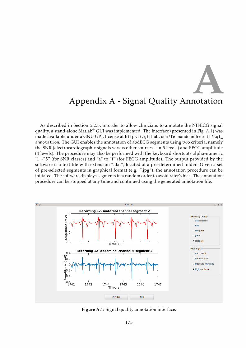
AAppendix A - Signal Quality Annotation
As described in Section 5.2.3, in order to allow clinicians to annotate the NIFECG signalquality, a stand-alone Matlab® GUI was implemented. The interface (presented in Fig. A.1) wasmade available under a GNU GPL license at https://github.com/fernandoandreotti/sqi_annotation. The GUI enables the annotation of abdECG segments using two criteria, namelythe SNR (electrocardiographic signals versus other sources – in 5 levels) and FECG amplitude(4 levels). The procedure may also be performed with the keyboard shortcuts alpha-numeric“1”-“5” (for SNR classes) and “a” to “f” (for FECG amplitude). The output provided by thesoftware is a text file with extension “.dat”, located at a pre-determined folder. Given a setof pre-selected segments in graphical format (e.g. “.jpg”), the annotation procedure can beinitiated. The software displays segments in a random order to avoid rater’s bias. The annotationprocedure can be stopped at any time and continued using the generated annotation file.
Figure A.1: Signal quality annotation interface.
175


BAppendix B - Fetal QRS Annotation
For the purpose of performing FHR/FHRV analyses, preferably exact annotations on theFQRS locations are necessary. Throughout this work, one of the objectives is to enable semi-automated methods that allow accurate FQRS detection and FHR estimation. In order toevaluate those methods, an expert-annotated gold-standard is necessary. With that in mind, astraightforward annotation scheme with four possible annotation markers (see Table B.1) wasintroduced as described below [410]:
1. The annotation procedure should (if possible) be performed by using simultaneouslyat least two different leads (preferably with different FECG polarities). That means,recognizing a fetal peak in one channel and comparing with the other if it is really a QRScomplex or an artifact;
2. Real-time RR generation function should be enabled at all times in providing a simplemethod for auto-assessment;
3. The chosen channels should be the ones on which the FECG appear to have the bestsignal quality (according to visual inspection). The used data can be either the rawsignal channels, pre-processed or processed leads. Other two channels for the annotatingprocedure may be chosen at any time due to quality fluctuation throughout the differentleads;
4. A peak is annotated (as normal peak ’N’) as long as it is visible in at least one of the twoabdominal channels. That, of course, if the form of the peak, QRS duration or heart rate isin accordance with FECG properties;
5. Peaks which are buried into noise or fetal peaks overlapped with maternal QRS complexesshould be annotated (as invisible peaks, or ’V’), as long as the number omitted beats in arow is not greater than two;
6. If the signal does not present a fetal R-peak due to signal quality issues, according to rules3 and 4, the annotation ”loss of FECG signal” in this area should be started (’B’ markershould be placed). This condition may be reversed (with an end marker ’E’) as soon as twofetal peaks in a row are once again visible. The stop for the annotation ”FECG signal loss”should be placed before these peaks;
7. Otherwise, no annotation is made.
177

Table B.1: Fetal QRS annotation markers used in this work [410].
Marker MeaningN normal, clearly recognizable fetal peak
Vprobable, yet invisible peak. This marker applies e.g.when the fetal complex is not visible due to an overlappingMQRS complex
Bbeginning of bad signal quality segment, where no fetalpeak is discernible
E end of bad signal quality segment
For the purpose of annotating FQRS data, the JAVA GUI developed by Grunitz [167] wasused. This GUI (shown in Fig. B.1) requires data to be in the Unisens format1 and allows thesimultaneous display of signals (e.g. MECG leads, raw, preprocessed or extracted abdECGs) andannotations (e.g. MQRS and FQRS). This versatile interface enables stretching and compressionon both X and Y axes, modification, deletion and inclusion of signals at all times, to facilitatethe GUI’s usage. Moreover, the GUI enables the presentation of live RR-intervals (see Fig. B.1),by taking the first derivative of “N” and “V” annotations, which enables specialists to quicklydetect and correct mistakes. The resulting annotated files are simple comma-separated files(“.csv”) containing markers and potential commentaries.
Maternal chest lead
Abdominal channels
Live RR-interval preview
12
3
Figure B.1: Java GUI used for FQRS annotation. In the screenshot are depicted (1) main menuwith open, close and save functions; (2) secondary menu with information to displayed plots;and (3) quick view of current file, annotation types and commentaries. In the screen are por-trayed a MECG chest lead, two abdominal leads (with FQRS annotations as vertical bars) andthe live RR viewer.
1 Unisens was developed at the FZI Research Center for Information Technology and the Institute for InformationProcessing Technology (ITIV) at the University of Karlsruhe. It is an open-source format available at: http:
//www.unisens.org/.
178
CAppendix C - Data Recording GUI
Recording NIFECG data in a clinical setup as the one described in this work is an arduoustask. The author’s first-hand experience with such problem lead to the development of a userinterface with the following goals:
• facilitate the recording procedure with an intuitive and simple interface, which is ex-tremely necessary when the medical expert is responsible for positioning a Doppler ultra-sound probe and be in charge of performing maneuvers (e.g. using the novel measurementprotocol described in Section 7.1.1);
• increase reproducibility of the recorded data regarding time duration and expert annota-tions relevant to further analysis. This is particularly important on the newly proposedrecording protocol (Section 7.1.1), during events such as paced breathing or blood pressureimpulse;
• improve consistency on the medical collection of patients’ information, such as limitingthe possible inputs for pathological conditions or placenta locations. This is important forthe posterior analysis on how this clinical conditions may influence the NIFECG analysis,as performed in Section 5.2.3.
For this purpose, a JAVA GUI (see Fig. C.1) was developed. The GUI was personalized tothe measurement system used in Leipzig and, after its opening, LabChart (ADInstruments’recording interface) is automatically started with a preset configuration file (“.adiset” extension)included in the GUI. The responsible expert is then prompted with the patient informationcollection form showed in Fig. C.1a. This form was developed through direct interaction withthe project partners from Leipzig and includes all the information usually collected by them.After the completion of this form and checking by the specialist, the recording may be initiatedand the user is prompted with the screen presented in Fig. C.1b. On the course of the recording,the expert is asked if the respiratory and blood pressure maneuvers (see Section 7.1.1) shouldbe performed by alerts (in case the step should be skipped), depicted in Fig. C.2a. The color ofthe interface is changed to indicate that a maneuver is being performed as detailed in Fig. C.2b.When the recording is finished, the expert is required to provide additional information on themeasurement that may be relevant for further analysis (e.g. interruptions or problems - seeFig. C.1c). Finally, the interface produces the following output data:
• collected patient information on tabular format (“.csv” extension), incrementally;
179
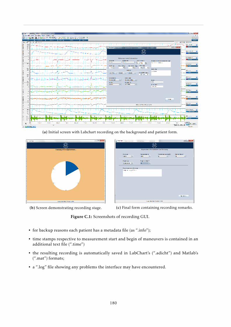
(a) Initial screen with Labchart recording on the background and patient form.
(b) Screen demonstrating recording stage. (c) Final form containing recording remarks.
Figure C.1: Screenshots of recording GUI.
• for backup reasons each patient has a metadata file (as “.info”);
• time stamps respective to measurement start and begin of maneuvers is contained in anadditional text file (“.time”)
• the resulting recording is automatically saved in LabChart’s (“.adicht”) and Matlab’s(“.mat”) formats;
• a “.log” file showing any problems the interface may have encountered.
180

(a) Alert
Resting Maneuver
(b) Color states during different recordingphases
Figure C.2: Chages to the GUI during physiological maneuvers.
181