Embed Size (px)
Citation preview

Externalities as Arbitrage∗
Benjamin Hebert†
July 30, 2021
Abstract
How can we assess whether macro-prudential regulations are having theirintended effects? If these regulations are optimal, their marginal benefit ofaddressing externalities should equal their marginal cost of distorting risk-sharing. These risk-sharing distortions will manifest as trading opportunitiesthat intermediaries are unable to exploit. Focusing in particular on arbitrageopportunities, I construct an “externality-mimicking portfolio” whose returnstrack the externalities that would rationalize existing regulations as optimal.I conduct a revealed-preference exercise using this portfolio and test whetherthe recovered externalities are sensible. I find that the signs of existing CIPviolations are inconsistent with optimal policy.
∗Acknowledgements: This paper builds on the work of and is dedicated to the memory ofEmmanuel Farhi. I would also like to thank Jonathan Berk, Eduardo Davila, Sebastian Di Tella,Wenxin Du, Darrell Duffie, Gary Gorton, Denis Gromb, Valentin Haddad, Barney Hartman-Glaser,Piero Gottardi, Bob Hodrick, Jens Jackwerth, Anton Korinek, Arvind Krishnamurthy, Matteo Mag-giori, Semyon Malamud, Ian Martin, Tyler Muir, Jesse Schreger, Amit Seru, Ludwig Straub, JeremyStein, Dimitri Vayanos, and seminar participants at the MIT Sloan Juniors Conference, Yale SOM,EPFL Lausanne, Stanford, UCLA, UC Irvine, Columbia Juniors Conference, Duke Macro Jam-boree, Gerzensee ESSFM, Barcelona FIRS, LSE, Wharton, HSE Moscow, and the Virtual FinanceSeminar for helpful comments, and in particular Hanno Lustig for many useful comments and PeterKondor for a helpful discussion. I would like to thank Michael Catalano-Johnson of SusquehannaInvestment Group for help with bounds on American option prices, Colin Eyre and Alex Rein-stein of DRW for help understanding SPX and SPY options, and Jonathan Wallen and ChristianGonzalez-Rojas for outstanding research assistance. All remaining errors are my own.†Stanford University and NBER. [email protected]

Following the great financial crisis (GFC), apparent arbitrage opportunities emerged
in financial markets. These arbitrage opportunities, such as the gap between the
federal funds rate and the interest on excess reserves (IOER) rate, or violations of
covered interest rate parity (CIP), are notable in part because they have persisted
for years after the peak of the financial crisis. Authors such as Du et al. (2018) have
argued that macro-prudential regulations put in place after the GFC have enabled
these arbitrages to exist and persist. If these apparent arbitrages opportunities are
made possible by macro-prudential regulations, does that imply that there is some-
thing wrong with the regulations? More generally, what can be learned from the
patterns of arbitrage across assets induced by regulation? Can we use these patterns
to assess whether macro-prudential regulations are having their intended effects?
Suppose we observe the price of an asset a that is traded by both intermediaries
and households, and the price of another asset a′ with identical payoffs that is traded
by intermediaries only. If the prices of a and a′ are not equal, an apparent arbitrage
exists. Such an opportunity can exist in equilibrium if intermediaries are bound
by a constraint that treats a and a′ differently (say, because it treats derivatives and
cash assets differently). Let us further suppose that this constraint exists because of
regulation– it is a leverage constraint, capital control, or some other kind of policy.
Now imagine that a household approaches an intermediary and wishes to buy
asset a. The intermediary contemplates selling asset a to the household and hedging
by purchasing asset a′. If the price of a is higher than the price of a′, this arbitrage
trade is profitable; the intermediary would execute the trade if unconstrained. From
this we can infer, as outside observers, that regulation is constraining the extent to
which the intermediary can sell the asset a to the household. That is, the regulation
1

is keeping the risks associated with asset a within the intermediary sector instead
of allowing those risks to be transferred to the household sector. We can then adopt
a macro-prudential viewpoint and ask whether or not it is desirable, from a social
perspective, to shift the holdings of asset a from households to intermediaries.
In this paper I develop a formal, multi-asset version of the argument above. The
procedure I develop takes the form of a revealed preference exercise. I ask: what ex-
ternalities would justify the distortions in risk-sharing I infer from various arbitrage
opportunities? Equivalently, what risks are pushed by regulation into the interme-
diary sector and what risks are pushed by regulation into the household sector? The
key step in the analysis is the construction of what I call the “externality-mimicking
portfolio.” This portfolio’s returns are an estimate of the externalities that would
justify the observed patterns of arbitrage, or equivalently an estimate of the effect
of regulation on risk-sharing between households and intermediaries.
I construct this portfolio using CIP violations. In the context of CIP violations,
the assets a and a′ are combinations of bond and exchange rate transactions. Em-
pirically, the sign of the observed arbitrage, as documented by Du et al. (2018), is
related to the direction of the carry trade– it is more expensive for the household
to execute the carry trade than it is for the intermediary to replicate the carry trade
using currency forwards. Consequently, I infer that the relevant regulatory con-
straint(s) have the effect of keeping carry trade risk within the intermediary sector,
instead of allowing intermediaries to transfer those risks to households. This result
is surprising given the risky nature of the carry trade.
The basic issue is that some CIP violations (e.g. AUD-USD and JPY-USD)
have the wrong sign. That is, because JPY appreciates and AUD depreciates vs.
2
USD in bad times, optimal policy should encourage intermediaries to be long JPY
and short AUD (i.e. short the carry trade). But the signs of the CIP violations are
such that they encourage intermediaries to be long the carry trade, taking on more
macro-economic risk. I speculate that this issue arises from an interaction between
leverage constraints (which do not consider the “sign” of a trade) and demand from
customers, as suggested by Du et al. (2018).
This conclusion does not rely on specific assumptions about which regulations
are binding in the case of CIP violations. This is desirable in light of the “alpha-
bet soup” of potentially relevant post-crisis regulations.1 That is, the methodology
developed in this paper is relatively model-agnostic and does not require strong as-
sumptions about the nature of the relevant regulation; in contrast, the traditional
approach of using a fully specified model necessarily involves such assumptions.
The procedure I develop has two key limitations. First, it assumes that the arbi-
trages under consideration are caused by regulation. The “anomalies” described by
Lamont and Thaler (2003) are violations of the law of one price between long-lived
assets, and can become larger before converging. Non-regulatory limits to arbitrage
(as in Shleifer and Vishny (1997)) might prevent intermediaries from eliminating
these anomalies. For this reason, I restrict my empirical analysis to short-dated
arbitrages (with a one-month or shorter horizon) which were insignificant prior to
the GFC. Second, the externality mimicking portfolio estimates the overall macro-
prudential effect of existing regulation, without identifying which regulations are
relevant. Some regulations, such as a leverage constraint, might be justified on
1In the context of CIP violations, Du et al. (2018) discuss leverage ratios, risk-weighted assetcalculations, stress tests, value-at-risk, the Volcker rule, liquidity coverage ratios, and the recentmoney market reform; most of these are implemented differently across jurisdictions, and some arecurrency- or country-specific for multi-national banks.
3

micro-prudential grounds, and yet have macro-prudential effects; likewise, redis-
tributive policies can have macro-prudential effects. When I use the returns of the
externality-mimicking portfolio to study the optimality of policy, I am implicitly
assuming that policymakers have a rich enough set of macro-prudential tools to
achieve their desired outcomes, even if that requires offsetting the macro-prudential
effects of non-macro-prudential policies.
I start from the general equilibrium with incomplete markets (GEI) framework
of Farhi and Werning (2016), which encompasses many existing studies of macro-
prudential policy.2 I augment this framework by distinguishing between two classes
of agents, “households” and “intermediaries,” as is standard when studying arbi-
trage (as in, e.g., Gromb and Vayanos (2002)). In this framework, optimal policy
equates the marginal benefits of addressing externalities with the marginal cost of
distorting risk-sharing. Under some additional assumptions about how policy is im-
plemented, these risk-sharing distortions will manifest themselves as arbitrage op-
portunities. To clarify the underlying mechanism and provide a concrete example,
I develop the example of capital controls, building on Fanelli and Straub (2019).
The central contribution of the paper uses the relationship between arbitrages
and externalities to construct what I call the “externality-mimicking portfolio.” The
returns of this portfolio are the projection of the externalities that would rational-
ize existing regulations onto the space of returns. Equivalently, they describe the
direction of the marginal risk-transfer between households and intermediaries un-
2I simplify the Farhi and Werning (2016) in several respects to clarify the exposition, but theprocedure I develop is applicable to the general framework. This framework is quite general, butdoes not span the set of all possible models. Appendix D briefly discusses how hidden trade, privateinformation, moral hazard, and other sources of inefficiency would affect the main results of thepresent paper.
4

der existing regulation. The portfolio can also be thought of as representing the
minimum difference between the household and intermediary SDFs necessary to
explain observed arbitrages (an analog of Hansen and Richard (1987)), or as the
portfolio that maximizes what I call the “Sharpe ratio due to arbitrage” (an analog
of Hansen and Jagannathan (1991)).
Using data on interest rates, foreign exchange spot and forward rates, and for-
eign exchange options, I construct an externality-mimicking portfolio. The weights
in this portfolio are entirely a function of asset prices; no estimation is required. If
policy is optimal, this portfolio’s returns track the externalities the social planner
perceives when considering transfers of wealth between the households and inter-
mediaries in various states of the world. Irrespective of whether policy is optimal,
the returns describe the direction of risk transfer between household and intermedi-
aries induced by policy. When its returns are positive (negative), the planner must
perceive positive (negative) externalities when transferring wealth from intermedi-
aries to households to rationalize existing policy. In “bad times,” we would expect
this portfolio to have negative returns, consistent with the idea that the planner
would like to encourage intermediaries to hold more wealth in these states.
I consider two definitions of “bad times.” First, intuitively, bad times can be
defined as times in which the intermediaries have a high marginal utility of wealth.
Using this definition, I show that it is sufficient to study the expected returns of the
externality-mimicking portfolio, and test if they are positive. Second, I define “bad
times” using the stress test scenarios developed by the Federal Reserve. I argue
that these tests are statements about when the Fed would like intermediaries to
have more wealth, and as a result the returns of the externality-mimicking portfolio
5

should be negative in the stress test scenarios.
However, I find that the expected return of the externality-mimicking portfolio
is generally negative, and that its returns in the stress tests are often positive. This
implies that the externalities that would justify current regulation are positive in bad
times; put another way, existing regulations are having the effect of retaining risk
within the intermediary sector. This is inconsistent with intuition and suggests that
regulations are not having their desired effect.
My theoretical framework builds on the GEI framework of Geanakoplos and
Polemarchakis (1986) and Farhi and Werning (2016). My example of capital con-
trols resembles both Fanelli and Straub (2019) and example 5.4 of Farhi and Wern-
ing (2016). In most theoretical models of macro-prudential policy (such as Farhi
and Werning (2016) and Davila and Korinek (2017)), a planner can implement pol-
icy using quantity constraints, agent-state-good-specific taxes, or some combination
thereof. In this paper, I focus on quantity constraints, which is both realistic, in the
sense that most regulation of banks takes this form, and enables the empirical ex-
ercise that follows. This paper is also related to Davila et al. (2012); both papers
attempt to measure how close existing allocations are to constrained efficiency.
My empirical work considers short-term arbitrages such as the fed funds/IOER
spread (Bech and Klee, 2011) and CIP violations (Du et al., 2018), and hence this
paper lies at the intersection of the theoretical literature mentioned above and the
empirical literature on arbitrage opportunities. The central and most surprising re-
sult of the paper is, in effect, that this intersection exists. The techniques I use to
characterize the externality-mimicking portfolio that links the theory with the data
build on Hansen and Richard (1987) and Hansen and Jagannathan (1991). There
6
is also a significant literature that studies CIP violations in the context of particu-
lar models (as opposed to the general GEI framework). Examples include Amador
et al. (2017); Andersen et al. (2019); Du et al. (2020); Gabaix and Maggiori (2015);
Ivashina et al. (2015). The framework I develop allows for the empirical analysis of
CIP violations within a relatively minimal theoretical structure, and hence enables
more general conclusions about the optimality or sub-optimality of policy.
1 Externalities and Arbitrage
I begin by outlining an endowment economy version of the economy studied by
Farhi and Werning (2016),3 with a specific asset structure that I will introduce be-
low. I will describe only the key aspects of the GEI framework; a more formal
presentation of the model can be found in appendix section C.
Let S1 be the set of future states, let s0 be the initial state, and define S = S1∪
{s0}. Let Js be the set of goods in each state s∈ S. The model will feature two sets of
agents, I (intermediaries) and H (households). An intermediary i ∈I will have
income Iis in state s ∈ S, and face prices {Pj,s} j∈Js , resulting in an indirect utility
in state s of V i(Iis,{Pj,s} j∈Js;s). Likewise, a household h ∈H will have income
Ihs and indirect utility V h(Ih
s ,{Pj,s} j∈Js;s). Each agent evaluates her expected utility
using a full-support “reference” probability measure {πrs}s∈S1 .4
The simplest interpretation of this setup is as a two-date model with multiple
goods in the second date, in which case these indirect utility functions are the result
3For simplicity, I also assume flexible prices and simpler constraints on transfers.4This probability measure is arbitrary; any differences between an agent’s subjective beliefs and
these probabilities can be incorporated into the state-dependent indirect utility function V .
7
of a standard consumer problem. The model can also be interpreted as having more
than two dates and a single consumption good at each date, in which case each
j ∈ Js corresponds to consumption at some date.5 The key assumption is that there
is at least one relative price in the future states s ∈ S1.
The incomes Iis and Ih
s are determined by the agents’ endowments and the al-
location of a set of assets. Let A be the set of assets in the economy, and let
Za,s({Pj,s} j∈Js) denote the payoff of asset a ∈ A in state s ∈ S1, given the goods
prices {Pj,s} j∈Js .6 Let Qa be the price of asset a ∈ A.
Intermediaries and households differ with respect to their ability to trade assets
in two ways. First, intermediaries can trade certain assets (the set AI ⊂ A) that
households cannot. Second, households cannot trade directly with each other, only
via intermediaries.7 Both features are standard in models of financial intermediation
such as Gromb and Vayanos (2002).
Consider a planner who can regulate asset allocations for each agent (denoted
Dia and Dh
a) and transfer wealth between agents in the initial state s0 (denoted T i and
T h).8 By regulating the asset allocations of and transfers to each agent, the planner
can influence the incomes Ihs and Ii
s. Define the income of household h in state s as
5See Farhi and Werning (2016) for several examples along these lines.6I adopt the convention that all assets are ’ex-dividend’ (have zero payoff in state s0), and that all
asset payoffs are homogenous of degree one in the goods prices.7Formally, A\AI is the union of a set of disjoint sets {Ah}h∈H , each containing assets tradable
by the household h and the intermediaries (but not other households). Note that multiple householdscan trade “the same” asset in the sense of payoffs; this formalism is simply a way of preventinghouseholds from trading directly with each other.
8The ability of the planner to transfer income in state s0 isolates the macro-prudential motivesof the planner (correcting externalities) from redistributive motives. This captures the idea that gov-ernments can use taxes and transfers for redistributive purposes while at the same time using macro-prudential regulations to correct externalities. See Appendix D for a discussion of the interpretationof the results in the absence of this assumption.
8

the sum of her endowment income, asset payoffs, and transfers,
Ihs = ∑
j∈Js
Pj,sY hj,s + ∑
a∈ADh
aZa,s({Pj,s} j∈Js)+T h1{s = s0},
where Y hj,s is the endowment of good j for household h in state s. Intermediary
income Iis is defined in similar fashion.
Regulations and Arbitrage Suppose that the planner regulates the trades of in-
termediaries but not households, and moreover does not constrain trade in the
intermediary-only assets AI for some intermediary i∗ ∈I . I will show below that
this is without loss of generality, in the sense that any optimal policy can be imple-
mented this fashion. For now, however, let us consider any regulations of this form,
optimal or sub-optimal.
Consider an asset tradable by households, a ∈ A \AI , and suppose there is an
asset tradable only by intermediaries, a′ ∈ AI , with identical cashflows (Za,s(·) =
Za′,s(·)). The household’s SDF will price the assets a ∈ A \AI . That is, for any
a ∈ A\AI , there exists an h ∈H such that
Qa = ∑s∈S1
πrs Mh,r
s Za,s({Pj,s} j∈Js), (1)
where Mh,rs denotes the household’s SDF.9 In contrast, regulations might constrain
intermediaries’ trade in a, in which case the intermediaries’ SDF will not price a.
9πrs Mh,r
s is the ratio of h’s marginal utility of income in state s ∈ S1, ∂
∂ IVh(I,{Pj} j∈Js ;s)|I=Ih
s,
relative to the marginal utility of income in state s ∈ S0. I have adopted the convention that thesubjective discount factor and subjective state probabilities are incorporated into the indirect utilityfunction.
9

The asset a′ ∈ AI , however, is priced by i∗,
Qa′ = ∑s∈S1
πrs Mi∗,r
s Za′,s({Pj,s} j∈Js), (2)
where Mi∗,rs is the SDF of i∗, and not necessarily by any household’s SDF.
If the regulations on intermediaries do not bind with respect to asset a, the inter-
mediaries’ SDF will price both assets, and the prices of a and a′ will be identical.
If regulations are binding with respect to asset a, meaning (by the definition of a
constraint ’binding’) that the intermediaries’ SDF does not price asset a, then the
prices of the assets a and a′ will not be identical. That is, an apparent arbitrage
opportunity (specifically, a law-of-one-price violation) will exist.
Apparent arbitrage opportunities of this form are driven by the difference be-
tween the household and intermediary SDFs,
Qa′−Qa = ∑s∈S1
πrs (M
i∗,rs −Mh,r
s )Za,s({Pj,s} j∈Js). (3)
This equation can be used in two ways. First, given a set of arbitrages (pairs
a ∈ A\AI and a′ ∈ AI with observable prices Qa and Qa′), it is possible to construct
an estimate of Mi∗,rs −Mh,r
s . This is one interpretation of what I call the “externality-
mimicking portfolio,” described in section 3 below. Second, given an estimate of
Mi∗,rs −Mh,r
s and an observable asset price Qa, this equation can be used to predict
Qa′ , even for assets without an intermediary-only replicating asset.10 That is, this
equation makes it possible to extrapolate the effects of regulation from assets for
10I use the terms replicating asset and replicating portfolio to describe an asset or portfolio withthe same payoffs, which may or may not have the same price.
10

which it is easily observed (e.g. CIP violations) to other traded assets. The differ-
ence between the SDFs, Mi∗,rs −Mh,r
s , summarizes the direction in which regulation
is pushing trade at the margin; if Qa′ < Qa, intermediaries are being discouraged by
regulation from selling asset a to households.
Before proceeding, I will note that these conclusions do not depend on the op-
timality of policy, only that policy is implemented by regulating intermediaries as
opposed to households, and by regulating trades between intermediaries and house-
holds but not between intermediaries. I view both of these assumptions as ap-
proximations of real world policy. First, macro-prudential regulations are usually
implemented by regulating banks, as opposed to attempting to directly regulate
the portfolios of households. Second, banks’ trades in products such as deriva-
tives are far less regulated than trades with households and firms. Interpreting the
intermediary-only assets as derivatives, the arbitrage arises due to the household’s
inability to trade derivatives and the regulatory constraints facing intermediaries,
exactly as suggested by e.g. Du et al. (2018).
This discussion has assumed that in the absence of regulation, intermediaries
would be free to trade both assets until their prices equalized. In the real world, it
is possible that non-regulatory constraints prevent arbitrage. In the fully specified
model of appendix section C, I consider this possibility, and conclude that the ar-
gument above holds for assets for which non-regulatory constraints do not bind. In
my empirical exercise, I address this issue by focusing on arbitrages that are short
maturity (circumventing limits-to-arbitrage issues) and absent prior to the GFC.
Lastly, observe that the logic above extends without modification from assets to
portfolios of assets. I will call an asset a ∈ A \AI “arbitrage-able” if there exists
11

a portfolio of assets in AI that replicate its payoff, regardless of the goods prices
that occur in equilibrium. That is, for any arbitrage-able asset, there exists portfolio
weights wa′(a) such that, for all states s ∈ S1 and all price levels {Pj,s},
Za,s({Pj,s}) = ∑a′∈AI
wa′(a)Za′,s({Pj,s}).
Let A∗ denote the set of arbitrage-able securities.
Optimal Policy Let us now consider what pattern of arbitrage should exist under
an optimal policy. Suppose that the planner can choose any asset allocations, trans-
fers, and goods prices for each state, subject to market clearing constraints for goods
and assets, a constraint that transfers sum to zero, and the constraints on feasible
asset allocations. Under these conditions and subject to a participation constraint
for intermediaries, suppose the planner maximizes household welfare. For a formal
definition of the problem, see definition 3 in appendix section C.
Let us consider in particular the market clearing constraint for good j in state s.
Let Xhj,s(I
hs ,{Pj′,s} j′∈Js) denote the demand function for good j by household h in
state s, and define X ij,s(·) as the same for intermediaries. Market clearing requires
that for each state s ∈ S and good j ∈ Js,
∑h∈H
(Xhj,s(I
hs ,{Pj′,s} j′∈Js)−Y h
j,s) = ∑i∈I
(X ij,s(I
is,{Pj′,s} j′∈Js)−Y i
j,s).
Let µ j,s be the multiplier on this constraint, scaled to the units of prices,11 and let
P∗j,s be the price chosen by the planner for good j in state s. The multiplier µ j,s can
11Converting from social marginal utility to price units requires scaling by a Pareto weight and anagent’s marginal utility; see section 2 below for an example.
12

be interpreted as the additional social cost of good j in state s above the price P∗j,s.
If the prices that clear markets are also the prices that maximize social welfare
(e.g. if the classic welfare theorems apply), the ratio of the social cost P∗j,s +µ j,s to
the private cost P∗j,s will be the same for all goods j ∈ Js within each state s ∈ S.12
In this case, the agents’ and the planner’s preferences are perfectly aligned, and the
solution to the constrained planner’s problem is also a competitive equilibrium.
However, if markets are incomplete, then generically, the solution to the con-
strained planner’s problem will not coincide with a competitive equilibrium (Geanako-
plos and Polemarchakis (1986)). If prices are rigid, or if there are constraints on
agents’ goods allocations that depend on prices, pecuniary externalities will lead
to generic constrained inefficiency regardless of whether markets are complete or
incomplete (Farhi and Werning (2016)). In these cases, the multipliers µ j,s are non-
zero, and the ratio of P∗j,s+µ j,s to P∗j,s is not the same for all goods within each state.
In what follows, I will focus on the incomplete markets case, but the results I derive
will hold regardless of whether the underlying source of inefficiency is incomplete
markets, nominal rigidities, prices in constraints, or some combination thereof.
To quantify these inefficiencies, I define “wedges” (following Farhi and Wern-
ing (2016)). The wedge τrj,s is the difference between the social/private cost ratio
for the good j ∈ Js in state s ∈ S1 and the average ratio for all goods in that state,13
πrs τ
rj,s =−
P∗j,s +µ j,s
P∗j,s+
1|Js| ∑
j′∈Js
P∗j′,s +µ j′,s
P∗j′,s.
12Only relative prices matter. If j0 is the numeraire (implying µ j0,s = 0 and P∗j0,s = 1), then theratio of social to private cost will be the same for all goods if and only if µ j,s = 0 for all goods.
13This definition of wedges is essentially the same as the one employed by Farhi and Werning(2016), adjusted for the difference between production and endowment economies and scaled by thereference measure πr
s . It is not necessary in what follows to define wedges for the state s0.
13

The wedge τrj,s is scaled by the probability measure πr
s > 0. In the applications I
consider, this measure is a risk-neutral measure or the physical probability measure.
The wedges τrj,s are defined in the context of this reference measure, and if defined
instead under an alternative reference measure πr′s would be rescaled, τr′
j,s =πr
sπr′
sτr
j,s.
The wedge is the difference between the first-order conditions of the planner and
of the agents– the latter do not account for effects of their demands on goods prices,
and these pecuniary externalities, due to market incompleteness, affect welfare. It
is positive if the social cost of a good is low relative to its price.
The wedges can be compensated for by transferring income in state s between
agents. Let h and i be two agents in the economy. Let XhI, j,s =
∂
∂ I Xhj,s(I,{P∗j′,s} j′∈Js)|I=Ih∗
s
be the change in h’s consumption of good j in state s if given a marginal unit of in-
come, holding prices constant, evaluated at the income Ih∗s and prices P∗j′,s that solve
the constrained planner’s problem, and let X iI, j,s be the same income effect for i. If
the wedge-weighted difference of these income effects,
∆h,i,rs = ∑
j∈Js
P∗j,sτrj,s(X
hI, j,s−X i
I, j,s),
is positive, transferring income from i to h in state s has a benefit, from the planner’s
perspective, because it alleviates externalities. I will call ∆h,i,rs the “externalities”
because they summarize this benefit.14
For goods j ∈ Js with positive wedges τrj,s, the social cost of the good is lower
than the price, and it is desirable to increase demand for the good. If XhI, j,s > X i
I, j,s,
then transferring income from i to h will indeed increase demand for the good. Sum-
14Farhi and Werning (2016) define an object τ iD,s, which is closely related, πr
s ∆h,i,rs = τh
D,s− τ iD,s.
14

ming these effects across goods determines the marginal benefit ∆h,i,rs of a transfer
of income from i to h in state s.
Under optimal policy, the marginal benefit of reallocating income between i
and h across the states s ∈ S1 is offset by a marginal cost– distorting risk-sharing.
Absent regulation, agents share risks by trading assets, ignoring externalities. The
planner, in contrast, distorts risk-sharing to address these externalities.
Consider an asset a ∈ A that can be freely traded by both i and h in the solution
to the constrained planner’s problem. The planner can reallocate the asset between
these agents; as a result, the marginal benefit of such a reallocation must equal
the marginal cost under optimal policies. Reallocating the asset between h and i
has a cost if it prevents those agents from equating their valuations of the asset.
The following proposition shows how the planner equates the marginal benefit of
reducing externalities and the marginal cost of distorting risk-sharing. Let Z∗a,s =
Za,s({P∗j,s} j∈Js) be the asset payoffs and let Mh,r,∗s and Mi,r,∗
s be the agents’ SDFs in
the solution to the planner’s problem.
Proposition 1. In the solution to the planner’s problem, for any agents h and i, and
any asset a ∈ A, if the planner is free to reallocate a between h and i, then
∑s∈S1
πrs ∆
h,i,rs Z∗a,s = ∑
s∈S1
πrs (M
i,r,∗s −Mh,r,∗
s )Z∗a,s. (4)
These results holds for both the endowment economy of appendix section C and the
production economy of section 4 of Farhi and Werning (2016).
Proof. See the appendix, section F.1, or Farhi and Werning (2016).
If there is a complete market of securities that can be freely reallocated by the
15

planner between h and i, then the externalities ∆h,i,rs must exactly equal the dif-
ference of the agents’ SDFs, Mi,r,∗s −Mh,r,∗
s . In this case, the externalities can be
non-zero if there are other agents who cannot trade in the complete securities mar-
ket (as shown in the example of section 2 below).15 In the incomplete markets case,
the externalities ∆h,i,rs are equal to the difference of the agents’ SDFs within the
span of the payoff space of the assets that can be reallocated between the agents.
That is, because the planner can move these assets between the agents, the planner
must equate the marginal benefit of doing so (alleviating the externalities) with the
marginal cost (distorting risk-sharing).
Implementation The marginal cost vs. marginal benefit tradeoff just described
arises from a planning problem in which the planner allocates assets for each of the
agents. Because the planner chooses each agent’s asset allocation, asset prices do
not enter the constrained planner’s problem. I next describe how the planner can
implement optimal policy using asset markets. In this implementation, there will
be a single price for each asset, and hence I will be able to discuss asset prices.
There is tension between assuming that each asset has a single price and the
results of Proposition 1. In the presence of externalities, Proposition 1 requires that
the willingness to pay for asset a of h be different from that of i, ∑s∈S1 πrs Mh,r,∗
s Z∗a,s 6=
∑s∈S1 πrs Mi,r,∗
s Z∗a,s. Consequently, h and i cannot both be free to trade the asset at the
price Qa. To implement optimal policy, the planner must place constraints on one
or both of the agents’ ability to trade the asset.16 These constraints are what I will
15The externalities can also be non-zero if prices are rigid or if prices enter constraints on agents’goods allocations, as discussed above.
16The planner could also use agent-specific taxes on asset holdings, so that the post-tax asset pricefaced by the agents is different even if the pre-tax price is the same. The FDIC fees charged to US
16

call macro-prudential policy; leverage restrictions are an example.
The planner has a great deal of latitude about the form of these constraints. The
agents, when trading the asset, consider both the asset price and the shadow cost of
the constraints (as in, e.g., Garleanu and Pedersen (2011) or Du et al. (2020)). As
long as these prices and shadow costs are consistent with Proposition 1, then the
resulting equilibrium will be constrained efficient. That is, the functional form of
the constraints does not matter, as long as the constraints generate the appropriate
shadow costs. In particular, the constraints could be a function of both asset prices
and portfolio choices (like a capital requirement), but this is not required.17
Under the financial intermediation structure I have assumed, proposition 2 be-
low shows it is without loss of generality for the planner to implement optimal
policy via portfolio constraints on intermediaries only. Because households trade
through intermediaries, by regulating the trade of intermediaries with each house-
hold and with each other, the planner can dictate the asset allocation for all agents.18
Now consider an arbitrage-able security a ∈ A∗, tradable by some household h.
Applying (1) to this asset and (2) to its replicating portfolio illustrates the relation-
ship between the arbitrage on asset a and the externalities.
Proposition 2. The planner can implement the solution to the constrained planning
problem using portfolio constraints on intermediaries only, and without constrain-
ing the trades of one intermediary, i∗ ∈I , in the intermediary-only assets AI .
banks are an example along these lines. I focus on quantity constraints because these appear morecommon in practice.
17For a formal definition of these portfolio constraints, see the appendix, Section §C.18This point also illustrates the limits of the Farhi and Werning (2016) framework, which does
not allow for either private information or hidden trade, both of which would limit the set of imple-mentable allocations. I discuss in appendix section D why my basic conclusions would continue tohold in the presence of private information or hidden trade.
17

In this implementation, for any arbitrage-able asset a ∈ A∗ that is tradable by
household h and that the planner is free to reallocate between h and i∗,
−Qa + ∑a′∈AI
wa′(a)Qa′︸ ︷︷ ︸arbitrage violation
= ∑s∈S1
πrs ∆
h,i∗,rs Z∗a,s︸ ︷︷ ︸
expected externality-weighted payoffs
. (5)
Proof. See the appendix, section F.2.
This equation demonstrates the tight connection under optimal policy between
arbitrage and the externalities the planner attempts to correct. To correct pecuniary
externalities, the planner must distort risk-sharing. Under the assumed structure of
financial intermediation, the planner can implement the optimal risk-sharing dis-
tortions by regulating intermediaries. In this implementation, certain assets will be
priced by households (because households are not directly regulated) while others
will be priced by intermediaries (because these assets are not tradable by house-
holds). For the subset of assets that are arbitrage-able (tradable by households with
an intermediary-only replicating portfolio), this implementation of optimal policy
will lead to an apparent arbitrage opportunity.
Strikingly, arbitrage is a generic feature of constrained efficient allocations (if
the planner implements the constrained efficient allocation in the manner described
by Proposition 2).19 The absence of arbitrage is not a sign of efficiency, but rather
a sign of inefficiency in the presence of incomplete markets. More specifically,
an arbitrage-able asset should be cheap relative to its replicating portfolio if its
payoffs occur mainly in states in which the planner would like to transfer wealth
19Generically, externalities are non-zero and are in the span of the payoff space of A∗.
18

from intermediaries to households.
The implementation described by Proposition 2 assumes that there exists an
intermediary who is completely unconstrained with respect to trade in the repli-
cating portfolio. This does not mean the intermediary is unregulated; it means
only that regulatory constraints do not bind for that intermediary with respect to
intermediary-only assets. Interpreting intermediary-only assets as derivatives, this
implementation assumes only that derivatives are priced by some intermediary.20
Lastly, note that these results inherit the generality of the Farhi and Wern-
ing (2016) framework. In particular, they allow for arbitrary heterogeneity across
agents in both preferences and endowments. I next provide a concrete example to
further illustrate the connection between externalities and arbitrage.
2 An Example of Externalities as Arbitrage
This section describes a version of Fanelli and Straub (2019) (see also example
5.4 of Farhi and Werning (2016)) to illustrate the meaning of Proposition 2. In
this example, a planner limits foreign-currency lending by intermediaries (i.e. uses
capital controls) to stabilize the real exchange rate. This creates a CIP violation
whose size and direction are determined by the externalities as in (5).
This example connects to the empirical exercise that follows in that it illustrates
how CIP violations can arise from optimal macro-prudential policy. However, this
example focuses on capital controls, and hence is more naturally interpreted as
concerning developing economies, whereas my empirical application focuses on
20It is likely more realistic to suppose regulations impact derivatives to a small degree; in thiscase, the result should be viewed as an approximation.
19

developed markets and bank regulation. I present this example because it more
transparently illustrates the principles behind the exercise.
There are two types of domestic households, Ricardians and non-participants
(H = {r,n}). In each state, there are two goods, tradable and non-tradable, Js =
{T,NT}. Both households have log utility preferences over a Cobb-Douglas aggre-
gate of tradables and non-tradables, with share parameter α on tradables.
The future state can be either good (g) or bad (b), S1 = {g,b}. Non-participants
are endowed with non-tradables YNT and tradables Y nT,s, with Y n
T,g > Y nT,b. Ricardian
households are endowed only with tradables Y rT . Only Y n
T,s varies across the states;
otherwise, the states are identical. Foreign intermediaries are risk-neutral, consume
tradables only, and have a large endowment of tradables in all states. The discount
factor for both households is β < 1, and is one for the intermediaries.
The tradables price is stable in the foreign currency, and the domestic price
index is stable in the domestic currency, and I will use the tradable good as the
numeraire (PT,s = 1). The exchange rate is therefore es = (PNT,s)1−α , Ricardians
can trade both a foreign-currency risk-free bond a f c, with Za f c,s(PNT,s) = 1, and a
domestic risk-free bond adc, with Zadc,s(PNT,s) = (PNT,s)1−α . Intermediaries can
trade both of these bonds, an intermediary-only foreign currency risk-free bond aI ,
and a currency forward aF at exchange rate F , ZaF ,s(PNT,s) = (PNT,s)1−α −F . The
bonds a f c and adc are both arbitrage-able: ZaI ,s(·) = Za f c,s(·) and F × ZaI ,s(·) +
ZaF ,s(·) = Zadc,s(·). Non-participants cannot trade any assets.
The planner’s problem is to maximize a weighted sum of household utility, sub-
ject to a participation constraint for the foreign intermediaries. Note that there is
a complete market traded between intermediaries and Ricardians, as the exchange
20

rate will vary across S1 = {g,b} and the domestic and foreign currency bonds will
have different returns. As a result, the participation constraint of the intermediaries
creates a unified budget constraint for the Ricardians.
Let πps be the physical measure,21 with π
ps0 = 1, let Ts0 be the transfer in s0 to
non-participants, and let λ p > 0 and λ r > 0 be Pareto weights. The planner solves
max{Ir
s≥0,Ins≥0}s∈S,{PNT,s≥0}s∈S,Ts0
∑h∈{r,n}
λh∑s∈S
πps V h
s (Ihs ,PNT,s),
subject to non-tradable market clearing, YNT = ∑h∈{r,p}
XhNT,s(I
hs ,PNT,s),∀s ∈ S,
the non-participants budget constraints, Ins = PNT,sYNT +Y n
T,s +1{s = s0}Ts0,∀s ∈ S,
and the Ricardian budget constraint, Irs0+π
pg Ir
g +πpb Ir
b ≤ 2Y rT −Ts0 .
The functional forms in this example lead to
V hs (I
hs ,PNT,s) =
β [ln(Ih
s )− ln(P1−α
NT,s )+(1−α) ln(1−α)] s ∈ {g,b},
ln(Ihs )− ln(P1−α
NT,s )+(1−α) ln(1−α) s = s0,
XhNT,s(I
hs ,PNT,s) = (1−α)
Ihs
PNT,s.
The market-clearing condition highlights the pecuniary externality present in
the model. If the Ricardian households sell a bond, reallocating income from the
states in S1 to the state s0, this will increase the price of the non-tradable good in
s0 and reduce the price in the states {g,b}. These price changes have an effect on
welfare because the poor households face incomplete (non-existent) markets. The
21Because intermediaries are risk-neutral, this is also the intermediaries’ risk-neutral measure.
21

additional social cost of the non-tradable good, µNT,s, is determined by the planner’s
first-order condition with respect to PNT,s, and can be written for s ∈ S1 as
µNT,s
P∗NT,s= β
Ins0
λ n πps (
λ n +λ r
Ins + Ir
s− λ n
Ins),
where λ n
Ins0
µNT,s is the multiplier on the goods market clearing constraint. In states in
which the income share of non-participants, Ins
Ins +Ir
s, is lower than the relative welfare
weight λ n
λ n+λ r , the planner would like to increase non-participant incomes. Because
non-participants are net sellers of non-tradables, it is desirable in this case to in-
crease PNT,s and the social cost of non-tradables is less than the private cost.22
The wedges are πps τ
pNT,s =−π
ps τ
pT,s =−
12
µNT,sP∗NT,s
, and the externalities simplify to
∆r,i,ps =−(1−α)
µNT,s
P∗NT,sπps= (1−α)β
Ins0
Ins(1− λ n +λ r
λ nIns
Ins + Ir
s).
Let us now consider the first-order conditions of the planner’s problem with
respect to Ricardian households’ income and with respect to the transfer Ts0 ,
βπps
λ r
Irs−(1−α)
µNT,s
P∗NT,s
λ n
Ins0
= πps
λ r
Irs0
−πps (1−α)
µNT,s0
P∗NT,s0
λ n
Ins0
= πps
λ n
Ins0
−πps (1−α)
µNT,s0
P∗NT,s0
λ n
Ins0
.
The transfer ensures that the goods market at date zero is efficient (µNT,s0 = 0).
Combining these equations produces the complete markets analog of (4),
πps (M
i,ps −Mr,p
s ) = πps ∆
r,i,ps , (6)
22Note that I have ignored tradable goods market clearing (Walras’ law), and without loss ofgenerality µT,s = 0.
22

where Mi,ps = 1 and Mr,p
s = βIrs0Irs
are the SDFs of the intermediaries and Ricardians,
respectively. Summing this equation weighted by the payoffs Za,s(P∗NT,s) gives a
version of (4) for log-utility households and risk-neutral intermediaries.
Moreover, the externalities must be non-zero in the solution to the planner’s
problem (and hence that competitive equilibria are inefficient). If the externalities
were zero, the income sharesIng
Ing+Ir
gand In
bInb+Ir
bwould both equal λ n
λ n+λ r , by (6) the Ri-
cardian incomes would be equal, Irg = Ir
b, and therefore the non-participant incomes
would be equal, Ing = In
b . Market clearing in non-tradables requires that if incomes
are identical across {g,b}, so are prices. But if the non-tradable price is the same in
g and b, non-participant income cannot be equal in those states by the assumption
that Y nT,g > Y n
T,b, and therefore the externalities must be non-zero.
More specifically, in the solution to the planner’s problem, the non-tradable
price will be lower in b than in g. Consequently, the domestic bond has a lower
return in b than in g. In the absence of regulation, in the competitive equilibrium
of this example the Ricardians will borrow from intermediaries using the foreign
currency bond (because β < 1 and the Ricardians have no income risk). The plan-
ner, to increase the price of non-tradables in state b relative to state g, would in-
stead prefer that Ricardians borrow from intermediaries using the domestic bond,
thereby increasing Ricardian income in b relative to g. A macro-prudential regula-
tion limiting the quantity of foreign-currency lending by intermediaries is one way
of implementing this outcome. Depending on parameters, the planner might also
limit the total amount of lending by intermediaries.
When the planner implements optimal policies as described in proposition 2, the
externalities ∆r,i,ps will manifest as arbitrages. The Ricardians will price the foreign-
23

currency and domestic-currency bonds a f c and adc. The foreign intermediaries will
price the intermediary-only (i.e. offshore) foreign-currency risk-free bond aI and
the currency forward aF . The resulting arbitrages are
QaI −Qa f c = πpg ∆
r,i,pg +π
pb ∆
r,i,pb , (7)
F×QaI +QaF −Qadc = πpg ∆
r,i,pg (P∗NT,g)
1−α +πpb ∆
r,i,pb (P∗NT,b)
1−α . (8)
The first is a difference between the price intermediaries use when borrowing or
lending with each other and the price they use when borrowing or lending to the
Ricardians. The second is a CIP violation that involves the domestic currency bonds
(the asset Ricardians can trade) and a replicating portfolio only intermediaries can
trade (the currency forward and the intermediary-only bond). These two arbitrages
closely resemble the arbitrages I study in the empirical exercise that follows.
3 The Externality-Mimicking Portfolio
Let us now adopt the perspective of a financial economist who observes asset prices,
and wants to know what externalities would justify the patterns of arbitrage in those
asset prices. Suppose the financial economist observes prices for a set of arbitrage-
able assets A∗ tradable by some household h, along with the prices of the corre-
sponding replicating portfolios of intermediary-only assets (e.g. derivatives). Fur-
ther suppose that the financial economist believes these arbitrages are caused by
regulation, and not by other frictions that are exogenous from the perspective of
24

regulators.23 In the context of the preceding example, A∗ = {a f c,adc} (the foreign
and domestic currency bonds), and h is a Ricardian household.
Suppose regulatory policy is implemented as described in section 1; then (3)
will hold. In this section, I show how (3) can be “inverted” to recover the difference
of the household and intermediary SDFs from asset prices. When the assets in A∗
form a complete market (i.e. in the example of the previous section), we can per-
fectly recover the difference of the SDFs from asset prices. When A∗ does not form
a complete market, we will instead recover the projection of the difference of the
SDFs onto the space of returns. In both cases, we will recover the (projected) differ-
ence of the SDFs by constructing a portfolio, the “externality-mimicking portfolio.”
The externality-mimicking portfolio’s returns track the externalities that would jus-
tify existing regulation as optimal (by Proposition 1).
For simplicity, I use the space of returns, Ra,s =Z∗a,sQa
, as opposed to the space
of payoffs, and therefore assume that every arbitrage-able asset and its replicating
portfolio have strictly positive prices.24 The return of an arbitrage-able asset a∈ A∗,
Ra,s, and the return of its replicating portfolio, RIa,s, are linked by the relationship
RIa,s = (1−χa)Ra,s, where
χa =−Qa +∑a′∈AI wa′(a)Qa′
∑a′∈AI wa′(a)Qa′(9)
is a scale-free measure of arbitrage. Intuitively, when the asset is cheaper than its
replicating portfolio, its returns are higher. Using this notation, we can rewrite (7)
23Plausible real-world examples include the post-GFC CIP violations (Du et al. (2018)) and thedifference between the federal funds rate and the IOER rate (Bech and Klee (2011)).
24This is without loss of generality if there is a risk-free arbitrage-able security, as one couldalways add some amount of the risk-free security to another other security to ensure that its price ispositive, while still ensuring that a replicating portfolio exists.
25

and (8) from the example in the previous section as
χa f c
χadc
=
πpg RI
a f c,g πpb RI
a f c,b
πpg RI
adc,g πpb RI
adc,b
·∆
r,i,pg
∆r,i,pb
.Now consider the portfolio of replicating portfolios (in the example, a portfolio
of the currency forward and intermediary-only bond, expressed as weights on the
replicating portfolios of the bonds traded by Ricardian households) defined by
θ ∗a f c
θ ∗adc
=
RI
a f c,g RIadc,g
RIa f c,b RI
adc,b
−1
·
π
pg RI
a f c,g πpb RI
a f c,b
πpg RI
adc,g πpb RI
adc,b
−1
︸ ︷︷ ︸inverse second moment matrix of RI
a,s
·
χa f c
χadc
.
This portfolio has returns that are equal to the externalities in each state,
∆r,i,pg
∆r,i,pb
=
RIa f c,g RI
adc,g
RIa f c,b RI
adc,b
·θ ∗a f c
θ ∗adc
.This portfolio, which is externality-mimicking portfolio in the context of the capital
controls example, is the projection of the externalities onto space of returns. In this
example, which features complete markets, the portfolio’s returns are the unique set
of externalities that would justify the observed pattern of arbitrage. More generally,
in the incomplete markets case, the externality-mimicking portfolio’s returns are a
(not unique) set of externalities that would justify the observed pattern of arbitrage.
These results are analogous to (and build on) the results of Hansen and Richard
(1987), who study the projection of an SDF onto the space of returns. Those au-
26
thors also show that their projection is equivalent to minimizing the variance of an
SDF, subject to the constraint that the SDF price a set of assets.25 Hansen and Ja-
gannathan (1991) then show that the portfolio whose returns are the projection of
the SDF is also the portfolio with the maximum available Sharpe ratio. Below, I
develop analogous interpretations of the externality-mimicking portfolio.
Constructing the externality-mimicking portfolio requires three ingredients:
1. A set of arbitrage-able assets A∗,
2. Prices for the arbitrage-able assets in A∗ and their replicating portfolios, and
3. Expected returns and a variance-covariance matrix for the assets in A∗.
I assume, to simplify the exposition, that A∗ includes a risk-free asset, whose
return is R f . Let RIf = (1− χ f )R f be the return on the replicating portfolio of
the risk-free asset, and let χA∗ be the vector of scaled arbitrages χa for the risky
assets in A∗. Let µA∗,r and ΣA∗,r be the mean vector and variance-covariance matrix
of the returns Ra,s for each risky arbitrage-able asset a ∈A∗, under some measure
πrs . Given µA∗,r and ΣA∗,r, the mean returns and variance-covariance matrix for the
returns RIa,s, µA∗,I,r and ΣA∗,I,r, are defined by the relationship RI
a,s = (1−χa)Ra,s. I
assume there are no redundant risky arbitrage-able assets (ΣA∗,r has full rank). From
these objects, I define the externality-mimicking portfolio.
Note, by definition, that the space of returns of the arbitrage-able assets is iden-
tical to the space of returns of the replicating portfolios. As a result, the externality-
mimicking portfolio can be defined as either a portfolio of the arbitrage-able assets
or as a portfolio of replicating portfolios. It is convenient for what follows to define
it as a portfolio of replicating portfolios; for the alternative, see appendix section E.
25This equivalence holds if the constraint that the SDF be positive does not bind.
27

Definition 1. The externality-mimicking portfolio is a portfolio of the replicating
portfolios of A∗, with weights on the risky replicating portfolios equal to
θA∗,r = (ΣA∗,I,r)−1(χA∗−χ f
µA∗,I,r
RIf
), (10)
and a weight on the risk-free replicating portfolio equal to
θA∗,rf =−(θ A∗,r)T µA∗,I,r
RIf
+1
(RIf )
2 χ f . (11)
Proposition 3 below demonstrates four facts about this portfolio. The first two
facts show that this portfolio is the projection of the externalities (under the assump-
tions of proposition 2) onto the space of replicating portfolio returns (i.e. the space
of returns for assets in A∗). The third fact shows that the return of the portfolio is
the difference between the household and intermediary SDFs, projected onto the
space of returns. The fourth fact shows that the portfolio maximizes the “Sharpe
ratio due to arbitrage,” which I define next.
Given an arbitrary portfolio θ of risky assets in A∗, consider both its Sharpe
ratio, SA∗,r(θ), and the Sharpe ratio of the replicating portfolio,26
SA∗,I,r(θ) =
θ T µA∗,I,r
RIf−∑a∈A∗ θa
(θ T ΣA∗,I,rθ)12
.
SA∗,r(θ) is defined similarly, with (µA∗,r,ΣA∗,r,R f ) in the place of (µA∗,I,r,ΣA∗,I,r,RIf ).
26The definition of the Sharpe ratio given here is signed, and might be scaled by the inverse ofRI
f when compared to other definitions of the Sharpe ratio. Note also that the portfolio weights θ
do not need sum to one (the units of θ are “dollars”, not percentages), and that the Sharpe ratio ishomogenous of degree zero.
28

Because the prices of the replicating portfolios are not the same as the prices
of the arbitrage-able assets, an allocation in dollars to arbitrage-able assets and the
same dollar asset allocation to the replicating portfolios are in fact claims to differ-
ent cashflows.27 I instead compare portfolios that are claims to the same cashflows
but perhaps have different prices. Define the portfolio transformation θ(θ) by
θa(θ) = (1−χa)θa.
This transformation converts an allocation in dollars at the replicating portfolio
prices to an allocation in dollars at the arbitrage-able asset prices.
I define the “Sharpe ratio due to arbitrage” as the difference between the Sharpe
ratio on a set of claims and the replicating Sharpe ratio of those same claims,
SA∗,I,r(θ) = SA∗,r(θ(θ))−SA∗,I,r(θ).
A little algebra shows that the Sharpe ratio due to arbitrage is the ratio of the excess
arbitrage, χA∗−χ fµA∗,I,r
RIf
, to the volatility of the portfolio,
SA∗,I,r(θ) =θ T · (χA∗−χ f
µA∗,I,r
RIf)
(θ T ΣA∗,I,rθ)12
.
I next summarize the properties of the externality-mimicking portfolio.
Proposition 3. Under the assumptions of proposition 2, the externality-mimicking
27For example, if both intermediaries and households can buy stocks at $1/share but householdspay $2/bond whereas intermediaries pay $1/bond, an allocation of $4 split equally between stocksand bonds means two shares and two bonds for the intermediaries, but two shares and one bond forthe households.
29

portfolio has the following properties:
1. The externalities are the return on the portfolio plus a zero-mean residual,
uncorrelated with the returns of all arbitrage-able assets a ∈ A∗: for all i ∈ I,
∆h,i∗,rs = ∑
a∈A∗RI
a,sθA∗,ra + ε
A∗,rs ,
∑s∈S1
πrs RI
a,sεA∗,rs = 0 ∀a ∈ A∗.
2. The variance of the externalities, ∑s∈S1 πrs (∆
h,i∗,rs − χ f
RIf)2, is weakly greater
than the variance of the externality-mimicking portfolio’s return, (θ A∗,r)T ΣA∗,I,rθ A∗,r.
3. Let mI,rs be any SDF that prices the replicating portfolios under the measure
πrs . Then mr
s = mI,rs +∑a∈A∗ RI
a,sθA∗,ra is the solution to the problem:
minm∈R|S1|
∑s∈S1
πrs (ms−mI,r
s )2 subject to
∑s∈S1
πrs msRa,s = 1 ∀a ∈ A∗.
4. The Sharpe ratio due to arbitrage of the externality-mimicking portfolio, SA∗,I,r(θ A∗,r),
is weakly greater than the Sharpe ratio due to arbitrage of any other portfolio
of replicating portfolios of the assets in A∗.
Proof. See the appendix, section F.3.
The first two claims follow from the least-squares projection. The third is the
analog of Hansen and Richard (1987), and shows that the estimated household SDF
mrs =mI,r
s +∑a∈A∗ RIa,sθ
A∗,ra is the one that makes the household’s and intermediary’s
SDFs as close as possible, subject to the constraint that it price the arbitrage-able
30

assets A∗ (and therefore differ sufficiently from mI,rs , which prices the replicating
portfolios).28 The fourth claim is the analog of Hansen and Jagannathan (1991),
and shows that the externality-mimicking portfolio is also the one the maximizes
the Sharpe ratio due to arbitrage.
The externality-mimicking portfolio is a reflection of what regulation is actually
accomplishing. Consider a state s in which the externality-mimicking portfolio has
a negative 10% return. If policy is optimal, the best linear prediction of the external-
ities in this state is negative 10%. That is, the planner would be indifferent between
being able to transfer ex-post one extra dollar from households to intermediaries in
state s and receiving an additional 10%×πrs dollars in the initial state s0.
The externality-mimicking portfolio is defined in the context of the reference
measure πr. In my empirical exercises, I focus on the intermediaries’ risk-neutral
measure, π i∗s = π
ps RI
f Mi∗,rs , and consider the physical (or actual) probability mea-
sure, π p, in robustness exercises. The two corresponding externalities are the “risk-
neutral externalities” ∆h,i∗,i∗s and the “physical externalities” ∆
h,i∗,ps , and are linked,
πps ∆
h,i∗,ps = π i∗
s ∆h,i∗,i∗s . This connection reflects the usual equivalence in asset pricing
between state-dependent preferences and beliefs. Using the risk-neutral externality-
mimicking portfolio has a particular advantage, which is that all expected returns
are equal to the risk-free rate, and hence observable. Moreover, options and quanto
option29 prices (which I presume are traded only by intermediaries) can reveal risk-
neutral variances and covariances (Kremens and Martin (2019)). If we consider
only arbitrage-able assets for which options and quantos are available (currencies
28That is, mrs maximizes a “market integration” measure along the lines of Chen and Knez (1995).
29A quanto option is an option that involves both an exchange rate and an asset (such as the S&P500). See appendix section A.4 or Kremens and Martin (2019) for details.
31

and the S&P 500), no estimation is required when constructing the risk-neutral
externality-mimicking portfolio. Using the physical measure, in contrast, requires
estimating both expected returns and a variance-covariance matrix.
The externality-mimicking portfolio reveals what externalities would justify ob-
served patterns of arbitrage under an optimal policy. The next step in our revealed
preference exercise is to ask whether the recovered externalities make sense. We
generally expect that externalities (and hence the mimicking portfolio returns) are
negative in “bad” states of the world. That is, governments seem tempted to bailout
intermediaries in bad states, not in good states. To test whether regulations are
consistent with this intuition, we need to define what we mean by “bad” states. I
consider two definitions, which result in two different tests. The first definition is
to define bad times as being bad for the intermediaries, which is to say that the
intermediaries’ SDF is high. The second definition involves studying a particular
situation– the “stress tests” conducted by the Federal Reserve– in which the regu-
lator is concerned about externalities, and would like intermediaries to have more
wealth. Presumably, the idea behind the stress tests is to ensure that intermediaries
have sufficient wealth in the stress scenario so as to avoid a bailout ex-post.
The first approach yields a simple test. The covariance of the intermediary SDF
and the risk-neutral externality-mimicking portfolio, under the physical measure, is
Covp(Mi∗,rs ,∆h,i∗,i∗
s ) =1
RIf(
χ f
RIf− ∑
s∈S1
πps ∆
h,i∗,i∗s )
=− 1RI
f(θ A∗,i∗)T · (µA∗,I,p−RI
f )+Covp(Mi∗,rs ,εA∗,i∗
s ).
If the externalities are negatively correlated with the intermediaries’ SDF, the ex-
32

pected excess return of the risk-neutral externality-mimicking portfolio under the
physical measure should be positive. Therefore, after constructing the externality-
mimicking portfolio, I will estimate its expected returns and ask whether or not they
are positive. The covariance term between the projection error and the intermediary
SDF shows that this test would be biased if there are components of the SDF that
are not spanned by the space of returns, and which are correlated with components
of the externalities that are also unspanned.
The second approach uses stress tests to identify a particular state (the stress test
scenario) in which externalities should be negative. The purpose of the stress test is
to verify that intermediaries have sufficient wealth in the stress scenario. To the ex-
tent that regulations achieve this goal, they must operate by inducing the intermedi-
aries to hold different assets and issue different liabilities than they otherwise would
have. Consequently, the intermediaries’ counterparties (the households) must also
hold different assets and issue different liabilities than they otherwise would have.
In other words, if the regulations act to raise intermediaries’ wealth in certain sce-
narios, they must lower the wealth of households in those scenarios (at least in
an endowment economy). That is, stress test scenarios are a statement when the
regulator perceives negative externalities associated with transferring wealth from
intermediaries to households (negative ∆h,i,rs ). Consequently, if the regulations are
having the desired effect, returns on the externality-mimicking portfolio in the stress
test scenario should be negative. This test is biased if the unspanned component of
the externalities is large in absolute value in the stress scenario.
33

4 Data
In this section, I describe the arbitrages, data sources, and additional assumptions I
use to conduct the tests described in the previous section.
The set of arbitrage-able securities A∗ should be limited to arbitrages induced
by regulation. I therefore focus on short maturity arbitrages, to avoid issues like the
classic limits to arbitrage argument (Shleifer and Vishny (1997)) and debt overhang
(Andersen et al. (2019)). This precludes many of the arbitrages documented in the
literature. I focus on arbitrages appeared after but not before the GFC, reasoning
that these arbitrages are likely to be induced by post-crisis regulatory changes. Two
classes of arbitrage that fit these criteria are the difference between the federal funds
rate and the IOER rate and CIP violations (Bech and Klee (2011); Du et al. (2018)).
Constructing the externality-mimicking portfolio requires determining what is
the “asset” a ∈ A∗ and what is the “replicating portfolio.” My framework offers two
ways of making this distinction: assets a ∈ A∗ are tradable by households, whereas
replicating portfolios are not, and intermediaries’ trades in assets a ∈ A∗ are regu-
lated, whereas trades in the replicating portfolio are not. To a first approximation,
the difference between “cash assets” and “derivatives” lines up with both of these
distinctions: derivatives are both less accessible to households and less regulated
under various leverage and capital requirements.
Consider first the fed funds/IOER arbitrage, which is the difference of two risk-
free rates. A bank can earn interest on excess reserves held at the Fed, whereas a
household cannot. If there is no meeting of the FOMC within the next month, the
bank is essentially guaranteed to earn one month’s worth of interest at the current
34

overnight rate.30 A household could instead purchase treasury bills, highly-rated
commercial paper, repo agreements (via money market funds), bank deposits, or
the like. I use 1-month OIS swap rates, which closely track the yields of one-month
maturity highly-rated commercial paper in the US, as a proxy for a risk-free rate
available to households that provides no liquidity benefits. These rates tend to be
higher than the rates on one-month constant maturity treasuries, but lower than
LIBOR rates (which may include credit risk).31 In the notation of the model, R f is
the one-month OIS swap rate, and RIf is the interest rate on excess reserves.
Next, consider CIP violations. Here, guided by the “cash vs. derivatives” heuris-
tic, I assume that households can purchase foreign-currency bonds, but cannot trade
derivatives.32 The asset a ∈ A∗ is a claim to one euro in one month, and households
can purchase this asset by spot exchanging dollars for euros and then purchasing
a risk-free euro-denominated bond. Following Du et al. (2020), I use OIS rates as
proxies for the risk-free rates available to households in various currencies. The
replicating portfolio involves an intermediary earning the dollar IOER rate for one
month and using a one-month FX forward to lock in the dollar/euro exchange rate.33
My data sample begins on January 4, 2011, and runs through March 12, 2018.
My sample is restricted to include only days on which the settlement of the one-
month currency forward occurs before the next FOMC meeting, excluding days
30In rare circumstances, the Fed might change the IOER rate between meetings, but such changeshave low ex-ante likelihood and are unlikely to materially alter the expected interest rate.
31For example, on August 19th, 2016, the one-month constant-maturity treasury rate was 27bps,the AA non-financial one-month commercial paper rates was 37bps, the one-month OIS rate was40bps, the IOER rate was 50bps, and one-month LIBOR was 52bps.
32That is, either the household cannot trade derivatives, or the transactions costs on derivativestrades for households are high enough that households cannot profitably execute the arbitrage.
33Implicitly, I am assuming that the default risk on the forward contract is negligible (or, to bemore precise, that the pricing data reflects forward rates available to a risk-free counterparty). Duet al. (2018) argue, persuasively in my view, that this risk is negligible.
35

with an FOMC meeting. Because the FOMC holds eight scheduled meetings each
year, roughly one quarter of all non-weekend days are included in the dataset.
My data on spot and forward exchange rates, FX options, and OIS rates are from
Bloomberg. I use the London closing time for all of these instruments, following
Du et al. (2018). I focus on the euro, yen, and pound, because these currencies are
major currencies that are modeled explicitly in the Federal Reserve’s stress test sce-
narios, and the Australian dollar, which plays a role in the “carry trade.” For details
of the data construction, see appendix section A.
Information on the “stress test” scenarios comes from the Federal Reserve’s
website.34 The “severely adverse” scenario described in the tests shows, among
other variables, the level of euro, yen, and pound, as well as the Dow Jones In-
dustrial Average, at a quarterly frequency. I collect both the one and four-quarter
percentage changes for each of the assets I study, and in my analysis will pretend
that these are returns that occur over a one-month horizon. For AUD, which is not
explicitly modeled in the stress test scenarios, I impute the returns in each stress
scenario by running a daily regression predicting AUD returns using the contempo-
raneous GBP, EUR, JPY, and stock returns over the preceding 720 days, and then
use these regression coefficients along with the one or four-quarter stress returns.
To conduct the tests described in the previous section, several additional as-
sumptions are required. To construct the risk-neutral externality-mimicking port-
folio, I require a full variance-covariance matrix under the risk-neutral measure. I
construct such a matrix from currency options on each currency possible currency
pair. For details, see appendix section §A. To estimate that portfolio’s expected
34https://www.federalreserve.gov/supervisionreg/dfa-stress-tests.htm
36

excess returns under the physical measure, an estimate of expected excess returns
is required. Motivated by Meese and Rogoff (1983) and the related literature, I
assume that exchange rates are random walks over my one-month horizon.
Table 1 presents the sample means and standard deviations of the arbitrage asso-
ciated with each currency and the risk-free arbitrage. Conceptually, these statistics
correspond to the term χa defined in (9). For example, for euros, it represents the
percentage difference in price, in dollars today, of purchasing a single euro one
month in the future by buying the euro at spot today and saving at OIS (the asset
a ∈ A∗), and obtaining the same euro one month in the future by savings at the
IOER rate and using a currency forward (the replicating portfolio). I also present
the difference between the dollar OIS rate and IOER (R f vs. RIf ). The arbitrages
have a one month horizon, but are scaled to annualized values.
This table also shows the option-implied volatility and correlations of each cur-
rency (with respect to the US dollar).35 Finally, the table reports the empirical
correlations between the currencies and both the SPDR ETF and the daily He et al.
(2017) (HKM) intermediary capital factor, and the quanto-implied correlations be-
tween the currencies and the S&P 500 (as in Kremens and Martin (2019), see ap-
pendix section A for details). A positive correlation means appreciation relative to
the dollar when the S&P 500 has positive returns.
From Table 1, we can observe several notable features of the data. First, inter-
mediaries are able to earn a higher rate of interest than households (IOER vs. OIS).
However, the positive sign on the euro, pound, and yen arbitrages implies that it
35A version of the table with physical measure estimated volatilities and correlations is in ap-pendix section B. The average volatilities and correlations are strikingly similar to their risk-neutralcounterparts.
37

is more expensive for intermediaries to use derivatives to purchase e.g. a euro one
month in the future in exchange for a dollar today than it is for intermediaries to use
products also available to households. The opposite pattern holds for the Australian
dollar. Note also that the euro and Australian dollar are positively correlated with
the S&P 500 and the HKM factor, while the yen is negatively correlated with the
S&P 500. Immediately, by Proposition 2, we can observe that the AUD and JPY
CIP violations do not have the expected sign, if either the S&P 500 or the HKM
factor is a reasonable proxy for the externalities. Figure 1 shows the time series of
the “risk-neutral” excess arbitrages, χa− χ f , for Australian dollar, euro, and yen.
Using the risk-neutral excess arbitrage, as opposed to the physical measure excess
arbitrage, eliminates the dependence on an estimate of expected returns.
5 Results
I first construct the risk-neutral externality-mimicking portfolio, using the euro,
Australian dollar, and yen assets, and a risk-free asset. This portfolio can be con-
structed at daily frequency using Definition 1 and data on the arbitrages and the
risk-neutral variance-covariance matrix implied by FX options prices. Figure 2 dis-
plays the time series of the portfolio weights on the risky assets (EUR, AUD, JPY).
A few patterns in the data are apparent. First, the portfolio is generally long
yen and euro and short AUD, and long currencies overall. That is, the portfolio is
short US dollars and short the carry trade.36 The “short US dollars” part is likely
to generate positive expected returns, whereas the “short the carry trade” generates
36In the terminology of Lustig et al. (2011), the portfolio is long the “level” factor and short the“slope” factor (the slope is with respect to interest rates).
38

negative expected returns, and this latter effect will dominate (see Table 2 below).
Interpreted through the lens of the model, this portfolio implies that a strong desire
to transfer wealth from households to intermediaries (negative externalities) coin-
cides with an appreciation of the US dollar and high returns for the carry trade.
If the planner would like to transfer wealth to intermediaries in “bad times,” the
first part seems sensible, in light of the safe haven role of the US dollar (see, e.g.,
Maggiori (2017)), but the second is surprising. Lustig and Verdelhan (2007) show
that negative carry trade returns are associated with falls in consumption, and we
would generally presume that these times are times when the planner would like
intermediaries to have relatively more wealth. Second, the noticeable spikes in the
euro and yen CIP deviations that occur around quarter- and year-end result in large
changes to the portfolio weight. This is not surprising, as there is no corresponding
large change in implied volatilities that would offset the effect. Interpreted through
the lens of the model, suddenly binding constraints could only be justified by large
changes in externalities, and hence in the externality-mimicking portfolio.
I next consider the predictions that this portfolio has about other arbitrages. I
deliberately excluded GBP from the set of currencies used to form the externality-
mimicking portfolio. This allows me to test whether the arbitrage predicted us-
ing the externality-mimicking portfolio is consistent with the arbitrage actually ob-
served for the dollar-pound currency pair. Formally, I compute
χGBP−χ f = ΣA∗,I,i∗GBP θ
A∗,i∗, (12)
where θ A∗,i∗ is the externality-mimicking portfolio in (10) and ΣA∗,I,i∗GBP is the co-
39
variance, under the intermediaries’ risk-neutral measure, between the dollar-pound
exchange rate and the risky assets used to form the externality-mimicking portfolio
(EUR, AUD, JPY). This is equivalent to computing the excess arbitrage under the
projected externalities, which coincides with the arbitrage under the true externali-
ties if there is no covariance between the pound and the error of the projection.
Figure 3 displays the results graphically. The actual excess arbitrage in pounds
is constructed from OIS rates in dollars and pounds, and the spot and forward
dollar-pound exchange rates (using excess arbitrage eliminates the dependence on
the IOER rate). The predicted excess arbitrage is constructed entirely from those
same variables in euros, AUD, and yen, along with options prices on all possible
currency pairs, which are used to both construct the externality-mimicking portfolio
(in the matrix ΣA∗,I,i∗) and to construct the covariances ΣA∗,I,i∗GBP . Note that the sets
of financial instruments used to construct the actual and predicted excess arbitrages
do not overlap. Nevertheless, the predicted and actual excess arbitrages track each
other, except near the end of 2011. The R2 of a regression of the actual arbitrage on
the predicted arbitrage, with no constant, is 83%. For predictions involving other
currencies, see appendix section B.1.
I next consider the expected return of this portfolio (the first test described in
the previous section). Intuitively, because the portfolio is generally short the carry
trade, the expected return on the portfolio is negative. This contradicts the intuition
that the externalities should be negatively correlated with the SDF. Figure 4 presents
the time series of expected excess returns on the portfolio, and Table 2 formally
tests whether the average expected return over my sample is greater than or equal
to zero (a one-sided test). I show results for the full sample, only for dates for
40

which the trade crosses a quarter-end, and only for dates for which the trade crosses
a year-end.37 I also formally test whether the quarter-end dates are different from
other dates, and whether the year-end dates are different from other quarter-end
dates. Both Bech and Klee (2011), for fed funds vs. IOER, and Du et al. (2018),
for CIP, have documented that the arbitrage spikes near quarter-ends. As these
results demonstrate, the problem of negative expected returns documented above is
particularly acute at quarter and year-ends.
I now turn to the second test, using the stress tests. Once per year, the Federal
Reserve describes a “severely adverse” scenario and requires banks to maintain
various leverage and capital ratios in this scenario. In Table 3, I present the returns
of the yen, euro, and stocks in the stress test scenarios, at both the one quarter and
four quarter horizons, for each stress test conducted. A general pattern emerges:
recent stress tests have involved sizable euro depreciations relative to the dollar,
and sizable yen appreciations. This pattern is consistent with the observation that,
during my sample, stock market declines tend to coincide with euro depreciation
and yen appreciation relative to the dollar, and that these sorts of correlations might
influence how the Federal Reserve constructs the stress test scenarios. The stock
return itself very negative in all of these scenarios.
The scenarios do not specify a return for the Australian dollar, presumably be-
cause it would be virtually impossible to the specify the returns of every asset a
bank might hold. I impute the return of the AUD using the stress tests returns on
euro, yen, and pounds (not shown in Table 3) and the stock market. Because of
the Australian dollar’s positive correlation with the stock market and negative cor-
37The trade crosses quarter/year end if the settlement dates of the spot and forward FX trades arebefore and after the end of some quarter/year, respectively.
41

relation with the yen, the imputed returns are quite negative. When banks calculate
their stress scenario returns, they likely perform a similar kind of imputation.
Each of the stress test scenarios is associated with a particular date (listed in
Table 3) which is the date at which the scenario starts. For each date in my sample
that is also within 180 calendar days of the stress test date, I report the returns
of the risk-neutral externality-mimicking portfolio under the associated stress test
scenario. Requiring that the relevant financial market data come from a day that is
within 180 days of the stress test date assigns almost all of the days in my sample
to a single stress test per date, dropping only a handful of days.
We should expect that the stress test returns of the externality-mimicking port-
folio are negative. However, this is not the case. At almost all points in time,
the portfolio is long low-interest-rate currencies (EUR and/or JPY) and short high-
interest-rate currencies (AUD), and as a result has positive returns in the stress sce-
nario, because the carry trade performs poorly in the stress scenario.
Table 4 formally tests whether returns are negative, averaging across dates near
a particular stress test. The p-values correspond to a one-sided test that the mean is
less than or equal to zero. I am able to reject the hypothesis that returns are negative
on average for all four stress test years beginning in 2014.
In summary, the risk-neutral externality-mimicking portfolio has negative ex-
pected returns and positive returns in the stress scenario, the opposite of what was
expected. On possible explanation, of course, is that the goal of regulation is to en-
courage intermediaries to take more, not less, macro-prudential risk, and regulatory
policy is accomplishing its goals. A more likely explanation, in my view, is that the
current regulatory apparatus is not accomplishing its macro-prudential objectives.
42

Du et al. (2018) shows that the direction of the CIP arbitrage across currencies
is predicted by the direction of the carry trade. A simple interpretation of this fact
is that households or their proxies want to do the carry trade, and intermediaries
are induced by the arbitrage to take the other side. Leverage constraints, such as
the “supplementary leverage ratio,” prevent the intermediaries from fully satisfy-
ing households’ demands. If this story is correct, households are trying to take
macro-economic risk and insure intermediaries from those risks, but regulation (the
leverage ratio) is limiting this risk transfer, which is the exact opposite of what an
optimal policy would do. Note that, under this interpretation, existing regulation
does not by itself determine the sign of the arbitrage. Instead, the sign of the ar-
bitrage under existing regulations arises from the interaction of customer demands
and regulatory constraints. This, however, is a policy choice; instead of encourag-
ing intermediaries to take more carry trade risk, regulation could be redesigned so
as to discourage intermediaries from taking carry trade risk.
For robustness, appendix section B presents three sets of additional results. The
first set uses the physical measure externality-mimicking portfolio instead of the
risk-neutral externality-mimicking portfolio in the stress test exercise. The esti-
mated physical and risk-neutral measure covariance matrices are similar, and the
stress test results do not depend on the choice of reference measure. See appendix
sections A.2 and B.2 for details on the construction of the portfolio and the results.
The second set of results incorporates an equity-based arbitrage between the
SPDR ETF and SPY options into the risk-neutral externality-mimicking portfolio.
The purpose of this robustness exercise is to demonstrate that the puzzling results
of the main analysis are not driven by the choice of arbitrages to include in the
43

portfolio. Including the SPDR-SPY arbitrage in the externality-mimicking portfo-
lio increases both the complexity and data requirements of the exercise, and the
noisiness of the results due to the imprecision in the measurement of the arbitrage.
For these reasons, I do not include it in the main analysis. With this arbitrage, the
results of the expected return test are broadly unchanged– expected returns are ro-
bustly negative, contrary to expectations. The results for the stress test are “better,”
in that more but not all of the stress returns are sharply negative.38 This effect is
driven by the combination of very negative equity returns in the stress scenario and a
small positive SPDR-SPY arbitrage (on average). The data is described in appendix
sections A.3 and A.4 and the results are presented in appendix section B.3.
The third set of results uses “carry” and “dollar” portfolios of currencies. These
results support the interpretation that the externality-mimicking portfolio is short
USD (which was expected) and short the carry trade (which was not expected). The
negative expected returns and positive returns in the stress scenario that I document
are due to the short carry aspect of the portfolio. See appendix sections A.5 and B.4
for details on the portfolios and the results.
6 Conclusion
There is a close connection between the externalities regulation attempts to ad-
dress and the arbitrage that regulation creates. Using this connection, we can assess
whether macro-prudential policies are achieving their objectives. I construct an
38These results taken together suggest that the stress returns might not be negative enough. Justbecause the returns in the stress scenario are negative does not mean macro-prudential regulation isworking optimally.
44

externality-mimicking portfolio, which tracks the difference between intermediary
and household SDFs, and hence the externalities that would rationalize existing pol-
icy. I argue that these externalities should negatively covary with the SDF, and be
negative in “stress” scenarios, and develop tests demonstrating that current data is
inconsistent with basic intuitions about the nature of optimal policies.
ReferencesManuel Amador, Javier Bianchi, Luigi Bocola, and Fabrizio Perri. Exchange rate
policies at the zero lower bound. The Review of Economic Studies, 2017.Leif Andersen, Darrell Duffie, and Yang Song. Funding value adjustments. The
Journal of Finance, 74(1):145–192, 2019.Morten L Bech and Elizabeth Klee. The mechanics of a graceful exit: Interest
on reserves and segmentation in the federal funds market. Journal of MonetaryEconomics, 58(5):415–431, 2011.
Zhiwu Chen and Peter J Knez. Measurement of market integration and arbitrage.The Review of Financial Studies, 8(2):287–325, 1995.
Eduardo Davila and Anton Korinek. Pecuniary externalities in economies withfinancial frictions. The Review of Economic Studies, page rdx010, 2017.
Julio Davila, Jay H Hong, Per Krusell, and Jose-Vıctor Rıos-Rull. Constrained ef-ficiency in the neoclassical growth model with uninsurable idiosyncratic shocks.Econometrica, 80(6):2431–2467, 2012.
Wenxin Du, Alexander Tepper, and Adrien Verdelhan. Deviations from coveredinterest rate parity. The Journal of Finance, 73(3):915–957, 2018.
Wenxin Du, Benjamin M Hebert, and Amy Wang Huber. Are intermediary con-straints priced? Working paper, National Bureau of Economic Research, 2020.
Sebastian Fanelli and Ludwig Straub. A theory of foreign exchange interventions.Working paper, 2019.
Emmanuel Farhi and Ivan Werning. A theory of macroprudential policies in thepresence of nominal rigidities. Econometrica, 84(5):1645–1704, 2016.
Xavier Gabaix and Matteo Maggiori. International liquidity and exchange rate dy-namics. The Quarterly Journal of Economics, 130(3):1369–1420, 2015.
Nicolae Garleanu and Lasse Heje Pedersen. Margin-based asset pricing and devi-ations from the law of one price. The Review of Financial Studies, 24(6):1980–2022, 2011.
45

John Geanakoplos and Heraklis M Polemarchakis. Existence, regularity, and con-strained suboptimality of competitive allocations when the asset market is in-complete. Uncertainty, information and communication: essays in honor of KJArrow, 3:65–96, 1986.
Denis Gromb and Dimitri Vayanos. Equilibrium and welfare in markets with finan-cially constrained arbitrageurs. Journal of financial Economics, 66(2):361–407,2002.
Lars Peter Hansen and Ravi Jagannathan. Implications of security market data formodels of dynamic economies. Journal of political economy, 99(2):225–262,1991.
Lars Peter Hansen and Scott F Richard. The role of conditioning information indeducing testable restrictions implied by dynamic asset pricing models. Econo-metrica: Journal of the Econometric Society, pages 587–613, 1987.
Zhiguo He, Bryan Kelly, and Asaf Manela. Intermediary asset pricing: New evi-dence from many asset classes. Journal of Financial Economics, 126(1):1–35,2017.
Victoria Ivashina, David S Scharfstein, and Jeremy C Stein. Dollar funding and thelending behavior of global banks. The Quarterly Journal of Economics, 130(3):1241–1281, 2015.
Lukas Kremens and Ian Martin. The quanto theory of exchange rates. AmericanEconomic Review, 109(3):810–43, 2019.
Owen A Lamont and Richard H Thaler. Anomalies: The law of one price in finan-cial markets. The Journal of Economic Perspectives, 17(4):191–202, 2003.
Hanno Lustig and Adrien Verdelhan. The cross section of foreign currency riskpremia and consumption growth risk. American Economic Review, 97(1):89–117, 2007.
Hanno Lustig, Nikolai Roussanov, and Adrien Verdelhan. Common risk factors incurrency markets. The Review of Financial Studies, 24(11):3731–3777, 2011.
Matteo Maggiori. Financial intermediation, international risk sharing, and reservecurrencies. American Economic Review, 107(10):3038–71, 2017.
Richard A Meese and Kenneth Rogoff. Empirical exchange rate models of theseventies: Do they fit out of sample? Journal of international economics, 14(1-2):3–24, 1983.
Andrei Shleifer and Robert W Vishny. The limits of arbitrage. The Journal ofFinance, 52(1):35–55, 1997.
46

Tables and Figures
Figure 1: Time Series of Excess Arbitrage
-100
010
020
030
0Ex
cess
Arb
. (bp
s)
1-Jan-11 1-Jan-12 1-Jan-13 1-Jan-14 1-Jan-15 1-Jan-16 1-Jan-17 1-Jan-18Date
JPY EURAUD
Notes: This figure plots the annualized excess arbitrage χa−χ f , as defined as in (9), for the yen, euro, and Australian dollar.These excess arbitrages are approximately equal to the one month OIS-based CIP violation vs. USD for those currencies.The sample is all US trading days from Jan 4, 2011 to March 12, 2018 that are at least one month before an FOMC meeting.
Figure 2: Externality-Mimicking Portfolio Weights
-50
510
15
1-Jan-11 1-Jan-12 1-Jan-13 1-Jan-14 1-Jan-15 1-Jan-16 1-Jan-17 1-Jan-18Date
JPY EURAUD
Notes: This figure plots the portfolio weights of the externality-mimicking portfolio (definition 1). The portfolio is con-structed using a set of arbitrage-able assets A∗ that contains the yen, euro, and Australian dollar, as well as a risk-free asset.The reference measure is the intermediaries’ risk-neutral measure, meaning that expected returns are equal to the IOER rateand the variance-covariance matrix is inferred from currency options. The sample is all US trading days from Jan 4, 2011 toMarch 12, 2018 that are at least one month before an FOMC meeting.
47

Figure 3: Actual vs. Predicted Excess Arbitrage in Pounds
050
100
150
200
Exce
ss A
rb. (
bps)
1-Jan-11 1-Jan-12 1-Jan-13 1-Jan-14 1-Jan-15 1-Jan-16 1-Jan-17 1-Jan-18Date
GBP Pred. GBP
Notes: This figure plots excess the annualized pound excess arbitrage χGBP− χ f , as defined in (9), along with the predictedvalue defined as in (12). The excess arbitrage is approximately equal to the one month OIS-based GBP-USD CIP violation.The risk-neutral externality-mimicking portfolio is constructed with an A∗ that contains the yen, euro, and Australian dollar,as well as a risk-free asset. The variance-covariance matrix used in the computation and the covariances with the pound areinferred from currency options. The sample is all US trading days from Jan 4, 2011 to March 12, 2018 that are at least onemonth before an FOMC meeting.
Figure 4: Risk-Neutral EMP Expected Returns
-200
-100
010
020
0Ex
cess
Ret
urn
(bps
)
1-Jan-11 1-Jan-12 1-Jan-13 1-Jan-14 1-Jan-15 1-Jan-16 1-Jan-17 1-Jan-18Date
Notes: This figure plots the excess expected return under the physical measure of the risk-neutral externality-mimickingportfolio (definition 1), under the assumption that currencies follow a random walk. The excess return is censored at +/-200bps to enhance readability. The risk-neutral externality-mimicking portfolio is constructed with an A∗ that contains theyen, euro, and Australian dollar, as well as a risk-free asset. The variance-covariance matrix used in the computation isinferred from currency options. The sample is all US trading days from Jan 4, 2011 to March 12, 2018 that are at least onemonth before an FOMC meeting.
48

Table 1: Summary Statistics for ArbitragePounds Euros Yen Aus.
DollarOIS-IOER
Arbitrage Mean (bps/year) 6.7 22.4 28.3 -15.4 -12.5Arbitrage SD (bps/year) 28.2 37.7 37.2 18.5 2.8
OI Vol. (bps/year) 859 950 977 1073 -OI Corr. with Pound/USD 1.00 0.56 0.22 0.47 -OI Corr. with Euro/USD 0.56 1.00 0.31 0.51 -OI Corr. with Yen/USD 0.22 0.31 1.00 0.26 -
Empirical Corr. with SPDR 0.23 0.10 -0.34 0.37 -Empirical Corr. with HKM 0.26 0.17 -0.31 0.31 -Implied Corr. with S&P 500 0.28 0.11 -0.29 0.50 -
N 444 444 444 444 444Notes: This table presents summary statistics for the sample of all US trading days from Jan 4, 2011 to March 12, 2018 atleast one month before an FOMC meeting. Arbitrage mean χa is defined using (9) for a claim to e..g. one euro in one month,priced in dollars today. The OIS-IOER arbitrage is the risk-free arbitrage, based on a claim to one dollar in one month.Arbitrage SD is the daily standard deviation of χa. OI Vol. and OI Corr. variables for currencies are the time-series meanof a daily series extracted from variance-covariance matrices implied by currency options. Empirical Corr. with SPDR andEmpirical Corr. with HKM are the time-series means of the correlations between the currency returns and the SPDR ETF(which tracks the S&P 500) and with the He et al. (2017) daily intermediary capital factor, as estimated on a rolling basisby the methodology described in appendix section A.2. Implied Corr. with S&P 500 is based on the time-series mean of thecurrency correlation with the S&P 500 extracted from quanto options and described in appendix section A.4.
Table 2: Risk-Neutral EMP Expected ReturnsN Mean (bps) Standard Deviation (bps) Test P-Value
Full Sample 444 -222 25.9 ≥ 0 0.0000Quarter-Ends 155 -431 69.7 ≥ 0 0.0000
Year-Ends 46 -1005 209.2 ≥ 0 0.0000QE - NQE -321 = 0 0.0000
YE - NYE QE -816 = 0 0.0000Notes: This table reports the excess expected return under the physical measure of the risk-neutral externality-mimickingportfolio (definition 1), under the assumption that currencies follow a random walk. The portfolio is constructed from an A∗
that contains the yen, euro, and Australian dollar, as well as a risk-free asset. The variance-covariance matrix used in thecomputation is inferred from currency options. The full sample is all US trading days from Jan 4, 2011 to March 12, 2018at least one month before an FOMC meeting. The quarter-end and year-end sub-samples are restricted to days on which aquarter- or year-end occurs between the spot FX settlement date and the one-month FX settlement date. The QE-NQE andYE-NYE QE rows report the mean difference between quarter-end vs. non-quarter-end dates and year-end vs. non-year-endquarter-end. Test indicates the hypothesis about the mean being tested, and P-Value reports the associated p-value.
49

Table 3: Stress Test “Severely Adverse” ScenariosEuro Stocks Yen AUD* *Imputed
Stress TestDate
One-QuarterReturn
Four-QuarterReturn
One-QuarterReturn
Four-QuarterReturn
One-QuarterReturn
Four-QuarterReturn
One-QuarterReturn
Four-QuarterReturn
9/30/12 -7.7 -15.4 -19.3 -51.5 2.8 -1.0 -8.8 -24.59/30/13 -14.3 -21.4 -26.5 -49.5 3.1 -1.1 -17.2 -28.79/30/14 -12.0 -13.4 -16.3 -57.1 7.6 6.5 -5.1 -17.2
12/31/15 -7.7 -13.9 -20.2 -50.7 2.7 5.1 -7.7 -18.312/31/16 -9.1 -11.9 -34.0 -49.7 3.3 7.5 -17.0 -24.112/31/17 -6.6 -10.9 -51.3 -62.8 11.7 4.6 -23.7 -32.9
Notes: This table reports the percentage changes in the level of the euro, yen, and the Dow Jones Total Stock Market Index(“Stocks”) during the first one or four quarters of the associated “Severely Adverse Scenario” from that year’s stress test.These percentage changes are treated as returns in my analysis. Stress Test Date lists the date on which that year’s scenariobegins. AUD shows the imputed return for the Australian dollar, using the imputation method described in the text.
Table 4: Risk-Neutral Returns in Stress ScenarioStressTestDate
N Mean(1Q,%)
S.D.(1Q,%)
P-value(1Q)
Mean(4Q,%)
S.D.(4Q,%)
P-value(4Q)
9/30/12 63 -0.8 0.3 0.9923 -1.8 1.0 0.95939/30/13 59 -0.9 0.4 0.9838 -2.1 0.7 0.99879/30/14 62 4.8 0.6 0.0000 9.9 1.0 0.000012/31/15 60 1.9 0.4 0.0000 4.5 0.8 0.000012/31/16 61 2.8 0.8 0.0000 7.0 1.2 0.000012/31/17 45 31.4 5.0 0.0000 28.6 4.3 0.0000
Notes: This table reports the mean and standard deviation of stress test scenario returns for the risk-neutral externality-mimicking portfolio portfolio. The risk-neutral EMP portfolio is constructed with an A∗ that contains the yen, euro, andAustralian dollar, as well as a risk-free asset. The variance-covariance matrix used in the computation is computed fromcurrency options prices. The sample is all US trading days from Jan 4, 2011 to March 12, 2018 that are at least one monthbefore an FOMC meeting and within 180 days of a stress test date. Each of these dates is assigned to the nearest stress testdate. N reports the number of dates assigned to each stress test, and P-Value reports the p-value associated with a one-sidedhypothesis test that the mean return is negative. Results are reported for both one-quarter (1Q) and four-return (4Q) returnsfrom the stress test scenarios.
50

Internet Appendix (For Online
Publication)
A Details on Data Construction
A.1 The Risk-Neutral Variance-Covariance Matrix
The risk-neutral variance-covariance matrix ΣA∗,I,i∗ is defined as variance-covariance
matrix, under the intermediaries’ risk-neutral measure, of the returns RIa,s. In the
case of currencies, these are the returns of investing at the IOER rate for one month
and using a currency forward to purchase, say, yen, and then immediately exchang-
ing back to dollars the spot rate. Let S j,t be the spot exchange rate of currency j per
dollar (e.g. euros per dollar, yen per dollar), and let Fj,t be the one-month forward
rate. The empirical analog of the return RIa,s is
R j,t = RIf ,t
Fj,t
S j,t+1,
where RIf ,t is the gross IOER rate accumulated over the one-month time horizon.
Note that, because RIf ,t is the risk-free rate available to intermediaries, we must
have E∗t [Fj,t
S j,t+1] = 1 where E∗t denotes expectations taken under the intermediaries’
risk-neutral measure.
To construct the risk-neutral variance-covariance matrix of currency returns, I
use daily, London-closing at-the-money 1-month implied volatilities from Bloomberg
for each currency pair. The volatilities are “percentage” volatilities from a log-
51

normal Garman and Kohlhagen (1983) model. If S j,t and S j′,t are two exchange
rates vs. the US dollar at time t (e.g. euros per dollar and yen per dollar), then
Cov∗t [∆s j,t+1,∆s j′,t+1] =12(V ∗t [∆s j,t+1]+V ∗t [∆s j′,t+1]−V ∗t [∆s j,t+1−∆s j′,t+1])
where ∆s j,t = ln(S j,t+1S j,t
) and Cov∗ and V ∗ denote the risk-neutral variance and co-
variance, respectively. Under the assumption of log-normality,
Cov∗t [S j,t
S j,t+1,
S j′,t
S j′,t+1] = E∗t [exp(−∆s j,t+1−∆s j′,t+1)]−E∗t [exp(−∆s j,t+1)]E∗t [exp(−∆s j′,t+1)]
=S j,tS j′,t
Fj,tFj′,t(exp(Cov∗t [∆s j,t+1,∆s j′,t+1])−1),
where F1,t and F2,t are the forward rates. It follows that
ΣA∗,I,ij, j′,t = (RI
f ,t)2(exp(
12(V ∗t [∆s j,t+1]+V ∗t [∆s j′,t+1]−V ∗t [∆s j,t+1−∆s j′,t+1]))−1).
In theory, I should make an adjustment to Bloomberg implied volatilities to use
a discount rate associated with the IOER rate, instead of the more standard OIS
rate. However, the difference amounts to about one basis point in the option price,
and hence is negligible. I have also experimented with more sophisticated methods
of computing the risk-neutral variance-covariance matrix (the “SVIX” method of
Martin (2017)). Such methods avoid log-normality assumptions at the expense of
additional data requirements and complexity, and have little impact on my results.
52
A.2 The Physical Expected Returns and Variance-Covariance
Matrix
Expected returns under the physical measure are required both to conducted the
expected returns test described in the text and to construct the physical measure
externality-mimicking portfolio. The latter also requires an estimate of the physical
measure variance-covariance matrix of returns.
As described in the text, I assume that currencies are random walks. Specifi-
cally, I assume log-normal exchange rates and that the log-exchange rate is a martin-
gale. The expected excess return of using the IOER rate and a forward to purchase,
say, one yen one month from now, is the determined by the difference between the
forward and expected exchange rate. That is,
µA∗,I,pj,t = RI
f ,tEt [Fj,t
S j,t+1],
where St+1 is the exchange rate in foreign currency per dollar, Ft is the one-month
forward rate, RIf ,t is the IOER rate accumulated over the next month, and expecta-
tions are taken under the physical measure. Under the stated assumptions,
µA∗,I,pj,t = RI
f ,tFj,t
S j,texp(
12
Vt [∆s j,t+1])
where Vt [∆st+1] is the conditional variance of the log change in the exchange rate.
Consequently, armed with an estimate for Vt [∆st+1], we can construct expected re-
turns.
I estimate a daily physical-measure variance-covariance matrix using an expo-
53

nentially weighted moving average of the daily series, with a decay factor of 0.97
(a procedure known as the “RiskMetrics” methodology, see for example Alexander
(2008)). This avoids using future information to estimate the variance-covariance
matrix. I initialize my variance and covariance estimates at the beginning of 2011
with the realized variance/covariance for 2010. I then scale my daily estimated
variance-covariance matrix to a one-month horizon.39
I use this estimated variance-covariance matrix of log returns both construct my
estimates of mean returns, as above, and to construct a variance-covariance matrix
for arithmetic returns, as described in appendix section A.1, under the assumption
of log-normality. In this case,
Covt [S j,t
S j,t+1,
S j′,t
S j′,t+1] = Et [exp(−∆s j,t+1−∆s j′,t+1)]−Et [exp(−∆s j,t+1)]Et [exp(−∆s j′,t+1)]
=µ
A∗,I,pj,t µ
A∗,I,pj′,t
(RIf ,t)
2
S j,tS j′,t
Fj,tFj′,t(exp(Covt [∆s j,t+1,∆s j′,t+1])−1)
and
ΣA∗,I,pj, j′,t =(µA∗,I,p
j,t µA∗,I,pj′,t )(exp(
12(Vt [∆s j,t+1]+Vt [∆s j′,t+1]−Vt [∆s j,t+1−∆s j′,t+1]))−1).
A.3 The SPDR ETF/SPY Option Arbitrage
In this section, I describe an equity-related arbitrage that I include in a robust-
ness exercise. The arbitrage I consider is an arbitrage between the SPDR S&P
500 ETF and options on that ETF, which trade on the CBOE under the ticker SPY.
39More sophisticated approaches that incorporate higher-frequency data might yield better results.See, for example, Ghysels et al. (2006).
54

This arbitrage is closely related to the classic index-future arbitrage involving S&P
500 futures (e.g. Chung (1991); MacKinlay and Ramaswamy (1988); Miller et al.
(1994)).
The arbitrage I study considers the cost of purchasing a share of the SPDR ETF
and holding it for one month as compared to the cost of purchasing that ETF via
put-call parity (by buying a call and selling a put with a one month horizon). The
ETF share itself is the arbitrage-able asset (both because it is easily purchased by
households and because regulations affect intermediaries’ trade in equity shares).
The intermediary, to replicate the ETF, can buy a call on the ETF, sell a put on the
ETF at the same strike, and invest enough cash at the IOER rate over the next month
to cover the exercise price of the put/call. Regardless of whether the ETF ends up
above or below the strike price, the intermediary will end up owning the ETF in one
month.
The particular details of this arbitrage are complicated by the fact that the SPY
options are “American” and not “European” options, meaning they can be exercised
at any time. I deal with this issue by employing the Margrabe (1978) bound on
American put prices, which in my setting (short time horizons and low interest
rates) is reasonably tight. I discuss this issue in more detail below.
The ETF and the replicating portfolio will generate identical payoffs as long as
there are no dividends over the course of the month (more precisely, that an ex-
dividend date does not occur within the month). The ETF has ex-dividend dates
quarterly, usually on the third Friday of March, June, September, and December.40
40The prospectus, available at https://us.spdrs.com/library-content/public/SPDR 500%20TRUST PROSPECTUS.pdf, describes the details of how theex-dividend dates are determined.
55

I therefore limit my sample to avoid these dates. This illustrates one of the two main
advantages the ETF-based arbitrage has over the traditional S&P 500 cash-futures
arbitrage. The stocks of the S&P 500 index pay dividends often, and hence most
studies of index arbitrage assume either perfect foresight of dividends or use a divi-
dend forecast, whereas no such assumptions are required for the ETF arbitrage. The
second advantage relates to transactions costs and stale prices. The traditional index
arbitrage involves buying and selling 500 stocks, generating substantial transactions
costs and exacerbating the issue that prices might not be synchronized. Using the
ETF, which is one of the most actively traded securities in the equity market and has
a very small bid-offer, mitigates many of these issues. Of course, synchronizing the
options prices and the ETF price is still critically important, as in Van Binsbergen
et al. (2012).
For this arbitrage, I am assuming that the costs associated with posting margin
on the options are negligible. That is, the margin is sufficiently small, and the
interest rate the intermediary receives on the posted margin sufficiently close to the
IOER rate, that these costs are negligible. This assumption is also, implicitly, being
applied to the margin required by counterparties in the OTC market for FX swaps
when studying CIP violations.
Because the SPY options are American, not European, I construct arbitrage
bounds as opposed to a single arbitrage measure. It is straightforward to observe
that an American call or put must be weakly more valuable than its European coun-
terpart, but the possibility of early exercise implies that this weak inequality might
be strict.
Let pa(K) ∈ A and ca(K) ∈ A denote the American put and American call of
56

strike K. Following the argument of Margrabe (1978), let pa(K) be an American
put option to exchange the ETF for an amount that grows at the IOER rate, K exp(t ·
ln(RIf )), where t is the time of the exchange. Because the option matures prior to
the next FOMC meeting, the IOER rate is assumed to be constant. Because the
intermediary is always indifferent between buying the ETF and the risk-free bond,
there is never any advantage to early exercise. Consequently, the put option pa has
the same value as a European style put option with the same expiry and a strike
KRIf . Moreover, because RI
f ≥ 1, the option pa is more valuable than the American
put pa. Hence, by no-arbitrage, the following inequalities hold for the American
put:
0≤ Qpe(K) ≤ Qpa(K) ≤ Qpa(K) = Qpe(KRIf ),
where pe(K) ∈ A is the European put of strike K. Using essentially the same argu-
ment, let ca be an American call option to buy the ETF in exchange for KRI
fexp(t ·
ln(RIf )) dollars at time t. Early exercise is again never optimal, and hence this call’s
value is equal to the European call with strike K and the same expiry. Moreover,
this call dominates the American call with strike K and the same expiry, and hence
early exercise is never optimal and the American and European calls have the same
value. That is,
Qca(K) = Qce(K),
where ce(K) ∈ A is the European call of strike K.
Let us now consider how to replicate the ETF. If I observed European options
57

prices, I would calculate the arbitrage, for any strike K, as
χe =Qce(K)−Qpe(K)+
KRI
f−Qe
Qce(K)−Qpe(K)+KRI
f
,
where Qe is the ETF price. Using the put inequalities derived above,
χe ≥ χe,min(K) =Qca(K)−Qpa(K)+
KRI
f−Qe
Qca(K)−Qpa(K)+KRI
f
,
and, for K′ = KRI
f,
χe ≤Qca(K′RI
f )−Qpa(K′)+K′−Qe
Qca(K′RIf )−Qpa(K′)+K′
. (13)
If RIf is sufficiently close to one (and one month’s worth of interest is indeed quite
small), these bounds will be tight.
One implementation issue that arises from these inequalities is that the strike
KRif is unlikely to be traded. However, by the convexity of call prices (another
cashflow dominance argument),
Qce(KRJf )≤ αQce(K1)+(1−α)Qce(K2)
for any K1 ≤ KRIf ≤ K2 such that αK1 + (1− α)K2 = KRI
f . Choosing K1 and
K2 to be as close as possible to KRIf generates the tightest bound. If KRI
f is
greater than the maximum traded strike Kmax, then Qce(KRIf )≤Qce(Kmax). Using these
bounds along with (13) generates an implementable upper-bound, which I will call
χe,max(K). Because these bounds must hold for all K, we are free to choose the
58

greatest lower bound and least upper bound from the set of available strikes.
Another empirical issue to consider in the implementation of this trading strat-
egy is whether to use bids and offers or mid-prices. Bid-offers are wide in options
markets, and likely substantially overstate the bid-offer associated with “delta one”
trades. That is, buying a call and selling a put together likely has a much smaller
bid-offer than doing those trades separately. For this reason, authors such as van
Binsbergen et al. (2019) use mid-prices. However, mid-prices can exhibit strange
behavior when bid-offers are particularly wide (which is why those authors use
outlier-robust methods of analysis). To deal with this issue, I consider only strikes
K with sufficiently small bid-offers. In particular, I restrict attention to values of
χe,min(K) which the difference between the mid-price and the lowest bound that
can be constructed from the various bids and offers is less than 0.05% of the spot
price Qe. Under this restriction, the lower bound χe,min(K) constructed from mid
prices is at most ˜5bps too high in the worse-case scenario. Similarly, I require that
the difference between χe,max(K) and the highest bound constructed from bids and
offers be less than 0.05% of Qe. From these two sets of valid strikes (one for χe,min
and one for χe,max), I choose the strikes that generate the tightest possible bounds
on χe.
After finding the maximum and minimum bounds, χe,min and χe,max, I define
the estimated arbitrage as
χe =
χe,min max(χe,min,χe,max)> χRF
χe,max min(χe,min,χe,max)< χRF
χRF otherwise.
59

In other words, I will assume that there is zero risk-neutral excess arbitrage (χe−
χRF) if this is possible, and assume the minimum amount, in absolute value terms,
if it is not possible.41 In practice, my final dataset never has χe = χRF , because the
bounds are sufficiently tight.
The dataset is a high-frequency (minute-level) dataset of options quotes pur-
chased from the CBOE DataShop. From this dataset (which contains quotes for
all minutes the exchange is open), I have extracted the five minutes on each day
immediately preceding the Bloomberg London closing time. On most days, this
is 12:55pm-12:59pm EST, although the EST hour moves around due the asyn-
chronous use of daylight savings time in the US and UK.
This dataset contains SPY options of many different expiries. Because I am
interested in one-month options (where one-month is defined based on FX trading
conventions) that do not cross an SPY dividend date, I restrict attention to expiries
between 21 and 58 days in the future. These cutoffs ensure expiries are roughly one
month and using these specific cutoffs simplifies the logic of determining whether
an expiry occurs after the next ex-dividend date on the SPY. I also require that each
expiry have at least eleven different strikes quoted to be included in the dataset.
The result of these restrictions and calculations is a dataset containing many esti-
mates of χe on each day (five minutes times the number of valid expiries). From this
set, for each day I search for minute/expiry pairs with non-missing data, expiries
that cross neither the next SPY ex-dividend date nor the next FOMC meeting, and
that have no arbitrage violations based on the bids and offers of options prices.42
Among the surviving minute/expiry pairs, I choose first the expiries that are clos-
41Note that, because I am using mid prices, it is possible to have χe,min > χe,max.42This last filter eliminates a few days with bad options quotes.
60

est to the FX market definition of one month, and then among those choose the
minute-expiry pair with the narrowest bid-offer for the relevant arbitrage bounds.
This procedures results in a unique value for χe on each day.
A.4 Expectations, Variance, and Covariance with the SPDR Ar-
bitrage
To use the SPY arbitrage described in the preceding sub-section in my exercise, I
require estimates of its variance and covariance with currency returns under both
the physical and risk-neutral measures, as well as an estimate of its expected return
under the physical measure.
I use, as an empirical analog of the one-month return RIa,s = (1−χa)Ra,s,
Re,t = (1−χe,t−1)Qe,t
Qe,t−1,
where Qe,t is the spot SPY price. Note that this definition does not include div-
idends, because I have restricted attention to dates on which dividends will not
occur over the next month.
To compute expected returns under the physical measure, I assume an equity
premium of 5% (roughly the average value of Martin (2017) in recent years). Al-
though many predictors of time-varying equity returns have been documented in the
literature, over a one-month horizon most of these predictors are quite weak, and it
seems reasonable to use an estimate of the unconditional equity premium. Under
this assumption,
µA∗,I,pt = (1−χe,t)(R f ,t−1+1.05∆t),
61

where ∆t is the time (in years) to the next month under the FX market convention
and R f ,t is the US OIS rate accumulated over that month.
To compute the physical-measure variance-covariance matrix, I use a daily se-
ries of surprise log-returns,
re,t = ln(Qe,t)− ln(Qe,t−1)− ln(R f ,t−1+1.05∆t),
consistent with how I construct surprise currency returns. I then use the same “Risk-
Metrics” methodology described in appendix section A.2.
I compute the risk-neutral variance-covariance matrix using the SVIX method
of Martin (2017) and data on quanto options from Markit (as in Kremens and Martin
(2019)). Applying the SVIX methodology of Martin (2017) (in particular, equation
(11) of that paper) to the SPY options data used to construct the arbitrage series χe,
I compute V ∗t−1[Qe,t
Qe,t−1], and then scale by (1−χe,t−1)
2 to compute the variance.
I extract covariances from data on quanto options on the S&P 500. A quanto
call option is, for example, the right to buy the S&P 500 for a fixed amount of euros
at a certain date. Such options are traded in OTC markets, and Markit provides a
pricing service to help dealers that trade these options mark their books. The prices
represent the (trimmed, cleaned) averages of prices submitted by participating deal-
ers. My data set includes prices for call and put options for all of currencies used in
this paper. Unfortunately, these options have a twenty-four month expiry (this is es-
sentially the only traded expiry), and the data is monthly rather than daily. I discuss
how I deal with both of these issues below. My use of the quanto options is also
complicated by the presence of arbitrage (CIP violations). I deal with this issue by
62
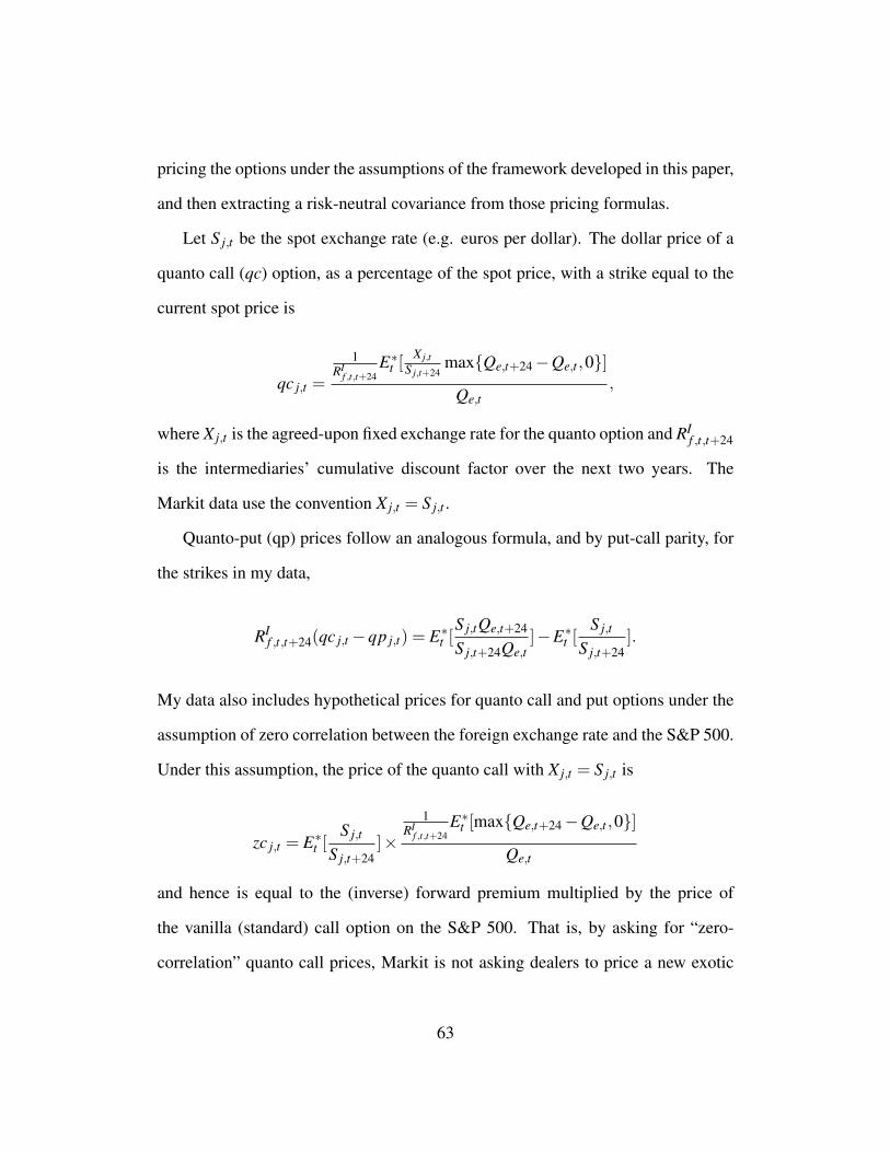
pricing the options under the assumptions of the framework developed in this paper,
and then extracting a risk-neutral covariance from those pricing formulas.
Let S j,t be the spot exchange rate (e.g. euros per dollar). The dollar price of a
quanto call (qc) option, as a percentage of the spot price, with a strike equal to the
current spot price is
qc j,t =
1RI
f ,t,t+24E∗t [
X j,tS j,t+24
max{Qe,t+24−Qe,t ,0}]
Qe,t,
where X j,t is the agreed-upon fixed exchange rate for the quanto option and RIf ,t,t+24
is the intermediaries’ cumulative discount factor over the next two years. The
Markit data use the convention X j,t = S j,t .
Quanto-put (qp) prices follow an analogous formula, and by put-call parity, for
the strikes in my data,
RIf ,t,t+24(qc j,t−qp j,t) = E∗t [
S j,tQe,t+24
S j,t+24Qe,t]−E∗t [
S j,t
S j,t+24].
My data also includes hypothetical prices for quanto call and put options under the
assumption of zero correlation between the foreign exchange rate and the S&P 500.
Under this assumption, the price of the quanto call with X j,t = S j,t is
zc j,t = E∗t [S j,t
S j,t+24]×
1RI
f ,t,t+24E∗t [max{Qe,t+24−Qe,t ,0}]
Qe,t
and hence is equal to the (inverse) forward premium multiplied by the price of
the vanilla (standard) call option on the S&P 500. That is, by asking for “zero-
correlation” quanto call prices, Markit is not asking dealers to price a new exotic
63

instrument but rather to report the levels of two standard contracts along with the
the price of the quanto call option.
Again by put-call parity,
RIf ,t,t+24(zc j,t− zp j,t) = E∗t [
S j,t
S j,t+24]E∗t [
Qe,t+24
Qe,t]−E∗t [
S j,t
S j,t+24],
where zp j,t is the zero-correlation quanto put price.
It follows that
E∗t [Qe,t+24
E∗t [Qe,t+24]
Fj,t,t+24
S j,t+24] =
1+ Fj,t,t+24S j,t
RIf ,t,t+24(qc j,t−qp j,t)
1+ Fj,t,t+24S j,t
RIf ,t,t+24(zc j,t− zp j,t)
, (14)
where Fj,t,t+24 is the two-year forward price.
As mentioned previously, the quanto dataset is a monthly dataset (with a few
missing observations) of 24-month expiry options. The goal of this exercise is to
extract one-month horizon covariances. To that end, I assume that correlations are
constant over horizon, so that I can extract a 24-month risk-neutral correlation and
then assume it is equal to the one-month correlation. I will use the most recent non-
missing observation for each currency. In the data, the correlations I extract move
slowly over time.
Ignoring these issues for a moment, the quantity of interest is
ΣA∗,I,i∗j,e,t = E∗t [Re,t+1R j,t+1]−E∗t [Re,t+1]E∗t [R j,t+1],
64

where R j,t is the intermediary currency return defined in A.1. This is
ΣA∗,I,i∗j,e,t = (1−χe,t)RI
f ,tE∗t [Qe,t+1]
QtCov∗t [
Qe,t+1
E∗t [Qe,t+1],
Fj,t
S j,t+1]
= (RIf ,t)
2Corr∗t [Qe,t+1
E∗t [Qe,t+1],
Fj,t
S j,t+1]V ∗t [
Qe,t+1
E∗t [Qe,t+1]]
12V ∗t [
Fj,t
S j,t+1]
12 . (15)
Under the assumption that correlations are constant across horizon,
Corr∗t [Qe,t+1
E∗t [Qe,t+1],
Fj,t
S j,t+1] =
Cov∗t [Qe,t+24
E∗t [Qe,t+24],
Fj,t,t+24S j,t+24
]
V ∗t [Qe,t+24
E∗t [Qe,t+24]]
12V ∗t [
Fj,t,t+24S j,t+24
]12
=E∗t [
Qe,t+24E∗t [Qe,t+24]
Fj,t,t+24S j,t+24
]−1
V ∗t [Qe,t+24
E∗t [Qe,t+24]]
12V ∗t [
Fj,t,t+24S j,t+24
]12. (16)
I compute risk-neutral variances V ∗t [Qe,t+24
E∗t [Qe,t+24]] and V ∗t [
Fj,t,t+24S j,t+24
] from Bloomberg at-
the-money 2-year at-the-money SPX implied volatilities and 2-year FX volatilities
(implicitly assuming log-normality). As discussed earlier, using an SVIX-based
calculation would avoid log-normality assumptions at the expense of increased data
requirements, computational complexity, and uncertainty related to bid-offers and
illiquidity of out-of-the-money options. Under an assumption of log-normality,
V ∗t [Qe,t+24
E∗t [Qe,t+24]] = exp(V ∗t [ln(Qe,t+24)])−1,
and likewise
V ∗t [Fj,t,t+24
S j,t+24] = exp(V ∗t [ln(S jt+24)])−1.
One last implementation concerns the intermediaries’ two-year discount factor,
RIf ,t,t+24. In the main text, I study only dates at least one month before an FOMC
65

meeting and use the IOER rate as the one-month rate. This approach does not allow
me to construct a two-year rate. For simplicity, I use instead the two-year OIS
rate and then add the sample mean spread between IOER and fed funds (see Table
1). This adjustment makes almost no difference to the estimated correlations. van
Binsbergen et al. (2019) offer a better approach: extracting a two-year intermediary
discount factor using “box” trades (put-call parity for different strikes). As with
the SVIX methodology, this approach is theoretically superior but increases data
requirements and concerns about issues related to illiquidity, bid-offer spreads, and
the like.
A.5 Construction of the Dollar and Carry Portfolios
As an additional robustness exercise, I construct an externality-mimicking portfo-
lio under the assumption that A∗ includes a risk-free asset and two portfolios of
currency trades, which I will refer to as dollar and carry.
These portfolios are portfolios of five developed-market currencies vs. the US
dollar. The five currencies (plus the US dollar) in the portfolio are: euro, yen,
pound, Australian dollar, and Canadian dollar. To select these currencies, I started
with the nine non-US-dollar G10 currencies. I removed the New Zealand dollar,
Swedish krona, and Norwegian Krone due to limited data availability for FX op-
tions and OIS swaps. I removed the Swiss franc both because of problems with its
OIS rate (discussed in Du et al. (2020)) and because of the pegging and de-pegging
events that occur during the sample period.
From these five non-USD currencies, I define the dollar and carry portfolios, in
the spirit of the factor approach of Lustig et al. (2011). Dollar is an equal-weighted
66

basket of the five currencies vs. USD. Note that this portfolio is short USD vs. these
other currencies, not long. This sign convention helps make the portfolio definition
consistent with the exercise in the main text. Carry is a long-short portfolio that
is long the two currencies with the smallest 1m forward premium and short the
two countries with the largest forward premium. For almost all of the sample, this
means long AUD and CAD and short JPY and EUR. To ensure a positive price, I
add some of the risk-free USD investment to the Carry portfolio. This has no effect
on the excess arbitrage χcarry− χRF , and hence no effect on resulting externality-
mimicking portfolio.
Expected returns and variance-covariance matrices for these portfolios can be
constructed from the assumed expected returns and variance-covariance matrices of
the individual currencies (as described in the previous parts of this appendix sec-
tion). Because some of the currencies in these portfolios are not explicitly modeled
in the stress tests, I impute returns using the same procedure used in the main text
for AUD.
B Additional Results
B.1 Predicted Arbitrage in Other Currencies
This sub-section presents the predicted vs. actual arbitrage using the risk-neutral
externality-mimicking portfolio for three additional currencies: CAD, CHF, and
SEK. These currencies have enough OIS swap and options data available to make
these predictions, although for both CHF and SEK the sample size is reduced.
67
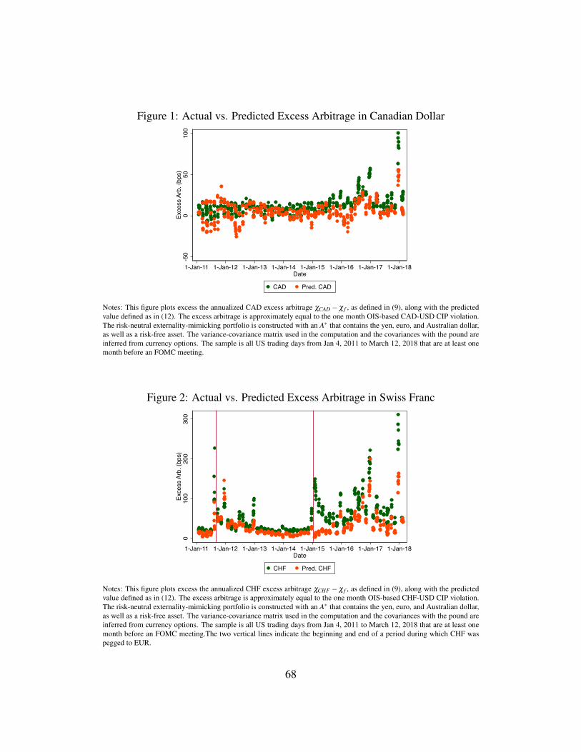
Figure 1: Actual vs. Predicted Excess Arbitrage in Canadian Dollar
-50
050
100
Exce
ss A
rb. (
bps)
1-Jan-11 1-Jan-12 1-Jan-13 1-Jan-14 1-Jan-15 1-Jan-16 1-Jan-17 1-Jan-18Date
CAD Pred. CAD
Notes: This figure plots excess the annualized CAD excess arbitrage χCAD− χ f , as defined in (9), along with the predictedvalue defined as in (12). The excess arbitrage is approximately equal to the one month OIS-based CAD-USD CIP violation.The risk-neutral externality-mimicking portfolio is constructed with an A∗ that contains the yen, euro, and Australian dollar,as well as a risk-free asset. The variance-covariance matrix used in the computation and the covariances with the pound areinferred from currency options. The sample is all US trading days from Jan 4, 2011 to March 12, 2018 that are at least onemonth before an FOMC meeting.
Figure 2: Actual vs. Predicted Excess Arbitrage in Swiss Franc
010
020
030
0Ex
cess
Arb
. (bp
s)
1-Jan-11 1-Jan-12 1-Jan-13 1-Jan-14 1-Jan-15 1-Jan-16 1-Jan-17 1-Jan-18Date
CHF Pred. CHF
Notes: This figure plots excess the annualized CHF excess arbitrage χCHF − χ f , as defined in (9), along with the predictedvalue defined as in (12). The excess arbitrage is approximately equal to the one month OIS-based CHF-USD CIP violation.The risk-neutral externality-mimicking portfolio is constructed with an A∗ that contains the yen, euro, and Australian dollar,as well as a risk-free asset. The variance-covariance matrix used in the computation and the covariances with the pound areinferred from currency options. The sample is all US trading days from Jan 4, 2011 to March 12, 2018 that are at least onemonth before an FOMC meeting.The two vertical lines indicate the beginning and end of a period during which CHF waspegged to EUR.
68

Figure 3: Actual vs. Predicted Excess Arbitrage in Swedish Krona
-100
010
020
0Ex
cess
Arb
. (bp
s)
1-Jan-11 1-Jan-12 1-Jan-13 1-Jan-14 1-Jan-15 1-Jan-16 1-Jan-17 1-Jan-18Date
SEK Pred. SEK
Notes: This figure plots excess the annualized SEK excess arbitrage χSEK − χ f , as defined in (9), along with the predictedvalue defined as in (12). The excess arbitrage is approximately equal to the one month OIS-based SEK-USD CIP violation.The risk-neutral externality-mimicking portfolio is constructed with an A∗ that contains the yen, euro, and Australian dollar,as well as a risk-free asset. The variance-covariance matrix used in the computation and the covariances with the pound areinferred from currency options. The sample is all US trading days from Jan 4, 2011 to March 12, 2018 that are at least onemonth before an FOMC meeting.
B.2 Results using the Physical Measure
This sub-section presents results using the physical-measure externality-mimicking
portfolio, as described in appendix section A.2. Table 1 presents a version of
the summary statistics table, with an estimated variance-covariance matrix in the
place of an option-implied variance-covariance matrix. I then present the portfolio
weights, predicted vs. actual GBP arbitrage, and stress test returns for the physical
measure. The results are similar to their counterparts from the main text.
69

Table 1: Summary Statistics for Physical-Measure ArbitragePounds Euros Yen Aus.
DollarOIS-IOER
Arbitrage Mean (bps/year) 6.7 22.4 28.3 -15.4 -12.5Arbitrage SD (bps/year) 28.2 37.7 37.2 18.5 2.8
Empirical Vol. (bps/year) 812 852 922 1046 -Empirical Corr. with
Pound/USD1.00 0.58 0.18 0.46 -
Empirical Corr. withEuro/USD
0.58 1.00 0.32 0.46 -
Empirical Corr. with Yen/USD 0.18 0.32 1.00 0.24 -Empirical Corr. with SPDR 0.23 0.10 -0.34 0.37 -Empirical Corr. with HKM 0.26 0.17 -0.31 0.31 -
N 444 444 444 444 444Notes: This table presents summary statistics for the sample of days from Jan 4, 2011 to March 12, 2018 at least one monthbefore an FOMC meeting. Arbitrage mean χa is defined using (9) for a claim to e..g. one euro in one month, priced in dollarstoday. The OIS-IOER arbitrage is the risk-free arbitrage, based on a claim to one dollar in one month. Arbitrage SD is thedaily standard deviation of χa. Empirical Vol. and Empirical Corr. variables for currencies are the time-series means of thecorrelations between the currency returns, as estimated on a rolling basis by the methodology described in appendix sectionA.2.. Empirical Corr. with SPDR and Empirical Corr. with HKM are the time-series means of the correlations between thecurrency returns and the SPDR ETF (which tracks the S&P 500) and with the He et al. (2017) daily intermediary capitalfactor, as estimated on a rolling basis by the methodology described in appendix section A.2.
Figure 4: Externality-Mimicking Portfolio Weights, Physical Measure
-4-2
02
46
1-Jan-11 1-Jan-12 1-Jan-13 1-Jan-14 1-Jan-15 1-Jan-16 1-Jan-17 1-Jan-18Date
JPY EURAUD
Notes: This figure plots the portfolio weights of the externality-mimicking portfolio (definition 1). The portfolio is con-structed using a set of arbitrage-able assets A∗ that contains the yen, euro, and Australian dollar, as well as a risk-free asset.The reference measure is the physical measure, meaning that expected returns calculated under the assumption that log ex-change rates are random walks and the variance-covariance matrix is estimated using the RiskMetrics methodology. Thesample is all US trading days from Jan 4, 2011 to March 12, 2018 that are at least one month before an FOMC meeting.
70

Figure 5: Actual vs. Predicted Excess Arbitrage in Pounds, Physical Measure
050
100
150
200
Exce
ss A
rb. (
bps)
1-Jan-11 1-Jan-12 1-Jan-13 1-Jan-14 1-Jan-15 1-Jan-16 1-Jan-17 1-Jan-18Date
GBP Pred. GBP
Notes: This figure plots excess the annualized pound excess arbitrage χGBP− χ f , as defined in (9), along with the predictedvalue defined as in (12). The excess arbitrage is approximately equal to the one month OIS-based GBP-USD CIP violation.The externality-mimicking portfolio is constructed with an A∗ that contains the yen, euro, and Australian dollar, as well as arisk-free asset. The reference measure is the physical measure, meaning that expected returns calculated under the assumptionthat log exchange rates are random walks and the variance-covariance matrix, as well as the covariances with the pound, isestimated using the RiskMetrics methodology. The sample is all US trading days from Jan 4, 2011 to March 12, 2018 thatare at least one month before an FOMC meeting.
Table 2: Physical Returns in Stress ScenarioStressTestDate
N Mean(1Q,%)
S.D.(1Q,%)
P-value(1Q)
Mean(4Q,%)
S.D.(4Q,%)
P-value(4Q)
9/30/12 63 -1.0 0.3 0.9998 -2.8 0.8 0.99959/30/13 59 -1.2 0.4 0.9963 -2.7 0.7 0.99999/30/14 62 6.2 0.9 0.0000 11.7 1.4 0.000012/31/15 60 1.9 0.5 0.0002 4.0 0.9 0.00012/31/16 61 1.4 0.8 0.0384 4.9 1.1 0.000012/31/17 45 35.7 4.3 0.0000 31.8 3.3 0.0000
Notes: This table reports the mean and standard deviation of stress test scenario returns for the physical-measure externality-mimicking portfolio portfolio. The physical measure EMP portfolio is constructed with an A∗ that contains the yen, euro,and Australian dollar, as well as a risk-free asset. The expected returns are calculated under the assumption that log exchangerates are random walks and the variance-covariance matrix is estimated using the RiskMetrics methodology. The sample isall US trading days from Jan 4, 2011 to March 12, 2018 that are at least one month before an FOMC meeting and within180 days of a stress test date. Each of these dates is assigned to the nearest stress test date. N reports the number of datesassigned to each stress test, and P-Value reports the p-value associated with a one-sided hypothesis test that the mean returnis negative. Results are reported for both one-quarter (1Q) and four-return (4Q) returns from the stress test scenarios.
71

B.3 Results including Equity Arbitrage
This sub-section presents results for a risk-neutral externality-mimicking portfolio
that incorporates JPY, EUR, and AUD arbitrages as well as the SPY-based arbitrage
described in appendix section A.3 and the risk-free rate arbitrage. The covariances
and expected returns under the physical measure used in this section are described
in appendix section A.4.
Table 3: Summary Statistics for Arbitrage including SPYPounds Euros Yen Aus.
DollarSPY OIS-
IOER
Arbitrage Mean (bps/year) 6.7 22.4 28.3 -15.4 5.4 -12.5Arbitrage SD (bps/year) 28.2 37.7 37.2 18.5 47.5 2.8
OI Vol. (bps/year) 859 950 977 1073 1566 -OI Corr. with Pound/USD 1.00 0.56 0.22 0.47 0.28 -OI Corr. with Euro/USD 0.56 1.00 0.31 0.51 0.11 -OI Corr. with Yen/USD 0.22 0.31 1.00 0.26 -0.29 -
Empirical Corr. with SPDR 0.23 0.10 -0.34 0.37 1.00 -Empirical Corr. with HKM 0.26 0.17 -0.31 0.31 0.66 -Implied Corr. with S&P 500 0.28 0.11 -0.29 0.50 1.00 -
N 444 444 444 444 312 444Notes: This table presents summary statistics for the sample of all US trading days from Jan 4, 2011 to March 12, 2018at least one month before an FOMC meeting. The SPY statistics are restricted to dates at least one month before a SPDRex-dividend date. Arbitrage mean χa is defined using (9) for a claim to e..g. one euro in one month, priced in dollars today.The OIS-IOER arbitrage is the risk-free arbitrage, based on a claim to one dollar in one month. Arbitrage SD is the dailystandard deviation of χa. OI Vol. and OI Corr. variables for currencies are the time-series mean of a daily series extractedfrom variance-covariance matrices implied by currency options, SPY options, and quanto options. Empirical Corr. withSPDR and Empirical Corr. with HKM are the time-series means of the correlations between the currency returns and theSPDR ETF (which tracks the S&P 500) and with the He et al. (2017) daily intermediary capital factor, as estimated on arolling basis by the methodology described in appendix section A.2. Implied Corr. with S&P 500 is based on the time-seriesmean of the currency correlation with the S&P 500 extracted from quanto options and described in appendix section A.4.
72
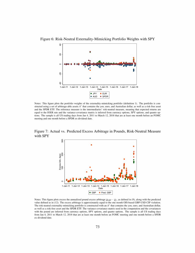
Figure 6: Risk-Neutral Externality-Mimicking Portfolio Weights with SPY
-40
-20
020
40
1-Jan-11 1-Jan-12 1-Jan-13 1-Jan-14 1-Jan-15 1-Jan-16 1-Jan-17 1-Jan-18Date
JPY EURAUD SPDR
Notes: This figure plots the portfolio weights of the externality-mimicking portfolio (definition 1). The portfolio is con-structed using a set of arbitrage-able assets A∗ that contains the yen, euro, and Australian dollar, as well as a risk-free assetand the SPDR ETF. The reference measure is the intermediaries’ risk-neutral measure, meaning that expected returns areequal to the IOER rate and the variance-covariance matrix is inferred from currency options, SPY options, and quanto op-tions. The sample is all US trading days from Jan 4, 2011 to March 12, 2018 that are at least one month before an FOMCmeeting and one month before a SPDR ex-dividend date.
Figure 7: Actual vs. Predicted Excess Arbitrage in Pounds, Risk-Neutral Measurewith SPY
010
020
030
0Ex
cess
Arb
. (bp
s)
1-Jan-11 1-Jan-12 1-Jan-13 1-Jan-14 1-Jan-15 1-Jan-16 1-Jan-17 1-Jan-18Date
GBP Pred. GBP
Notes: This figure plots excess the annualized pound excess arbitrage χGBP− χ f , as defined in (9), along with the predictedvalue defined as in (12). The excess arbitrage is approximately equal to the one month OIS-based GBP-USD CIP violation.The risk-neutral externality-mimicking portfolio is constructed with an A∗ that contains the yen, euro, and Australian dollar,as well as a risk-free asset and the SPDR ETF. The variance-covariance matrix used in the computation and the covarianceswith the pound are inferred from currency options, SPY options, and quanto options. The sample is all US trading daysfrom Jan 4, 2011 to March 12, 2018 that are at least one month before an FOMC meeting and one month before a SPDRex-dividend date.
73

Table 4: Risk-Neutral EMP Expected Returns with SPYN Mean (bps) Standard Deviation (bps) Test P-Value
Full Sample 312 -111 43.3 ≥ 0 0.0053Quarter-Ends 93 -425 125.9 ≥ 0 0.0005
Year-Ends 23 -1495 439.9 ≥ 0 0.0013QE - Full -447.0 = 0 0.0000YE - QE -1421 = 0 0.0000
Notes: This table reports the excess expected return under the physical measure of the risk-neutral externality-mimickingportfolio (definition 1), under the assumption that currencies follow a random walk and with a 5% equity risk premium. Theportfolio is constructed from an A∗ that contains the yen, euro, and Australian dollar, as well as a risk-free asset and theSPDR ETF. The variance-covariance matrix used in the computation is inferred from currency options, SPY options, andquanto options. The full sample is all US trading days from Jan 4, 2011 to March 12, 2018 at least one month before anFOMC meeting and one month before a SPDR ex-dividend date. The quarter-end and year-end sub-samples are restrictedto days on which a quarter- or year-end occurs between the spot FX settlement date and the one-month FX settlement date.The QE-NQE and YE-NYE QE report the mean difference between quarter-end vs. non-quarter-end dates and year-endvs. non-year-end quarter-end. Test indicates the hypothesis about the mean being tested, and P-Value reports the associatedp-value.
Table 5: Risk-Neutral Portfolio with SPY, Returns in Stress ScenarioStressTestDate
N Mean(1Q,%)
S.D.(1Q,%)
P-value(1Q)
Mean(4Q,%)
S.D.(4Q,%)
P-value(4Q)
9/30/12 28 -1.9 0.6 0.9989 -6.0 2.1 0.99569/30/13 52 -0.7 1.5 0.6786 -17.7 4.3 0.99999/30/14 54 2.5 1.3 0.0304 -14.3 2.0 1.000012/31/15 53 0.1 0.7 0.4302 0.4 1.6 0.414212/31/16 55 -23.4 1.6 1.0000 -30.2 2.1 1.000012/31/17 41 0.0 5.4 0.5013 -16.7 4.8 0.9994
Notes: This table reports the mean and standard deviation of stress test scenario returns for the risk-neutral externality-mimicking portfolio portfolio. The risk-neutral EMP portfolio is constructed with an A∗ that contains the yen, euro, andAustralian dollar, as well as a risk-free asset and the SPDR ETF. The variance-covariance matrix used in the computationis computed from currency options prices, SPY options, and quanto options. The sample is all US trading days from Jan 4,2011 to March 12, 2018 that are at least one month before an FOMC meeting, one month before a SPDR ex-dividend date,and within 180 days of a stress test date. Each of these dates is assigned to the nearest stress test date. N reports the numberof dates assigned to each stress test, and P-Value reports the p-value associated with a one-sided hypothesis test that the meanreturn is negative. Results are reported for both one-quarter (1Q) and four-return (4Q) returns from the stress test scenarios.
B.4 Results with Dollar and Carry Portfolios
This sub-section presents for a risk-neutral externality-mimicking portfolio that in-
corporates “Carry” and “Dollar” arbitrages, as well as a risk-free rate arbitrage.
74
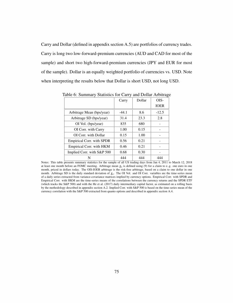
Carry and Dollar (defined in appendix section A.5) are portfolios of currency trades.
Carry is long two low-forward-premium currencies (AUD and CAD for most of the
sample) and short two high-forward-premium currencies (JPY and EUR for most
of the sample). Dollar is an equally weighted portfolio of currencies vs. USD. Note
when interpreting the results below that Dollar is short USD, not long USD.
Table 6: Summary Statistics for Carry and Dollar ArbitrageCarry Dollar OIS-
IOER
Arbitrage Mean (bps/year) -44.1 8.6 -12.5Arbitrage SD (bps/year) 31.4 23.3 2.8
OI Vol. (bps/year) 835 680 -OI Corr. with Carry 1.00 0.15 -OI Corr. with Dollar 0.15 1.00 -
Empirical Corr. with SPDR 0.56 0.21 -Empirical Corr. with HKM 0.46 0.21 -Implied Corr. with S&P 500 0.68 0.30 -
N 444 444 444Notes: This table presents summary statistics for the sample of all US trading days from Jan 4, 2011 to March 12, 2018at least one month before an FOMC meeting. Arbitrage mean χa is defined using (9) for a claim to e..g. one euro in onemonth, priced in dollars today. The OIS-IOER arbitrage is the risk-free arbitrage, based on a claim to one dollar in onemonth. Arbitrage SD is the daily standard deviation of χa. The OI Vol. and OI Corr. variables are the time-series meanof a daily series extracted from variance-covariance matrices implied by currency options. Empirical Corr. with SPDR andEmpirical Corr. with HKM are the time-series means of the correlations between the currency returns and the SPDR ETF(which tracks the S&P 500) and with the He et al. (2017) daily intermediary capital factor, as estimated on a rolling basisby the methodology described in appendix section A.2. Implied Corr. with S&P 500 is based on the time-series mean of thecurrency correlation with the S&P 500 extracted from quanto options and described in appendix section A.4.
75
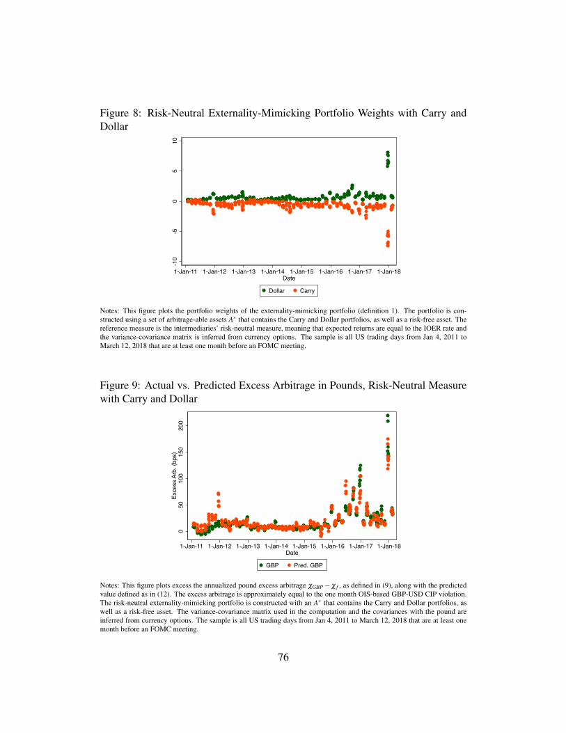
Figure 8: Risk-Neutral Externality-Mimicking Portfolio Weights with Carry andDollar
-10
-50
510
1-Jan-11 1-Jan-12 1-Jan-13 1-Jan-14 1-Jan-15 1-Jan-16 1-Jan-17 1-Jan-18Date
Dollar Carry
Notes: This figure plots the portfolio weights of the externality-mimicking portfolio (definition 1). The portfolio is con-structed using a set of arbitrage-able assets A∗ that contains the Carry and Dollar portfolios, as well as a risk-free asset. Thereference measure is the intermediaries’ risk-neutral measure, meaning that expected returns are equal to the IOER rate andthe variance-covariance matrix is inferred from currency options. The sample is all US trading days from Jan 4, 2011 toMarch 12, 2018 that are at least one month before an FOMC meeting.
Figure 9: Actual vs. Predicted Excess Arbitrage in Pounds, Risk-Neutral Measurewith Carry and Dollar
050
100
150
200
Exce
ss A
rb. (
bps)
1-Jan-11 1-Jan-12 1-Jan-13 1-Jan-14 1-Jan-15 1-Jan-16 1-Jan-17 1-Jan-18Date
GBP Pred. GBP
Notes: This figure plots excess the annualized pound excess arbitrage χGBP− χ f , as defined in (9), along with the predictedvalue defined as in (12). The excess arbitrage is approximately equal to the one month OIS-based GBP-USD CIP violation.The risk-neutral externality-mimicking portfolio is constructed with an A∗ that contains the Carry and Dollar portfolios, aswell as a risk-free asset. The variance-covariance matrix used in the computation and the covariances with the pound areinferred from currency options. The sample is all US trading days from Jan 4, 2011 to March 12, 2018 that are at least onemonth before an FOMC meeting.
76

Table 7: Risk-Neutral EMP Expected Returns with Carry and DollarN Mean (bps) Standard Deviation (bps) Test P-Value
Full Sample 444 -151 20.7 ≥ 0 0.0000Quarter-Ends 155 -315 56.1 ≥ 0 0.0000
Year-Ends 46 -763 169.9 ≥ 0 0.0000QE - Full -252 = 0 0.0000YE - QE -638 = 0 0.0000
Notes: This table reports the excess expected return under the physical measure of the risk-neutral externality-mimickingportfolio (definition 1), under the assumption that currencies follow a random walk. The portfolio is constructed from anA∗ that contains the Carry and Dollar portfolios, as well as a risk-free asset. The variance-covariance matrix used in thecomputation is inferred from currency options. The full sample is all US trading days from Jan 4, 2011 to March 12, 2018at least one month before an FOMC meeting. The quarter-end and year-end sub-samples are restricted to days on whicha quarter- or year-end occurs between the spot FX settlement date and the one-month FX settlement date. The QE-NQEand YE-NYE QE report the mean difference between quarter-end vs. non-quarter-end dates and year-end vs. non-year-endquarter-end. Test indicates the hypothesis about the mean being tested, and P-Value reports the associated p-value.
Table 8: Stress Test “Severely Adverse” ScenariosCarry* *Imputed Dollar* *Imputed
Stress TestDate
One-QuarterReturn
Four-QuarterReturn
One-QuarterReturn
Four-QuarterReturn
9/30/12 -7.4 -16.5 -4.1 -11.69/30/13 -8.9 -13.1 -10.5 -16.59/30/14 -2.1 -10.5 -3.2 -7.7
12/31/15 -3.8 -10.5 -4.1 -8.812/31/16 -11.3 -18.2 -7.9 -11.012/31/17 -23.6 -25.9 -8.0 -14.2
Notes: This table reports the imputed returns of the Carry and Dollar portfolios during the first one or four quarters of theassociated “Severely Adverse Scenario” from that year’s stress test, using the imputation method described in the text. StressTest Date lists the date on which that year’s scenario begins.
77

Table 9: Risk-Neutral Portfolio with Carry and Dollar, Returns in Stress ScenarioStressTestDate
N Mean(1Q,%)
S.D.(1Q,%)
P-value(1Q)
Mean(4Q,%)
S.D.(4Q,%)
P-value(4Q)
9/30/12 63 0.9 0.4 0.0144 0.4 0.9 0.32349/30/13 59 -1.8 0.4 1.0000 -2.9 0.6 1.00009/30/14 62 0.1 0.1 0.1707 3.9 0.6 0.000012/31/15 60 -0.5 0.1 0.9992 0.1 0.3 0.396512/31/16 61 3.7 0.6 0.0000 7.9 1.0 0.000012/31/17 45 27.5 4.4 0.0000 20.6 3.0 0.0000
Notes: This table reports the mean and standard deviation of stress test scenario returns for the risk-neutral externality-mimicking portfolio portfolio. The risk-neutral EMP portfolio is constructed with an A∗ that contains the Carry and Dollarportfolios, as well as a risk-free asset. The variance-covariance matrix used in the computation is computed from currencyoptions prices. The sample is all US trading days from Jan 4, 2011 to March 12, 2018 that are at least one month before anFOMC meeting and within 180 days of a stress test date. Each of these dates is assigned to the nearest stress test date. Nreports the number of dates assigned to each stress test, and P-Value reports the p-value associated with a one-sided hypothesistest that the mean return is negative. Results are reported for both one-quarter (1Q) and four-return (4Q) returns from thestress test scenarios.
C General Equilibrium with Intermediaries
This appendix section more formally describes the environment outlined in section
1.
The economy has a set of future states, S1, and an initial state, s0. Let S =
S1 ∪{s0} denote the set of all states, and let Js be the set of goods in each state
s ∈ S. The government can transfer income between agents in the initial state, s0,
but not any other state, and these transfers must sum to zero. The goods available
in each state are denoted by the set Js.
Households h ∈H maximize expected utility,
∑s∈S
Uh({Xhj,s} j∈Js;s),
78

where Uh({Xhj,s} j∈Js ;s) is the utility of household h in state s, inclusive of the house-
hold’s rate of time preference and the probability the household places on state s.
I will assume non-satiation for at least one good in each state, implying that each
household places non-zero probability on each state in S1, and that the utility func-
tions are differentiable. Note that I will refer to each h as “a household,” and assume
price-taking; nothing would change if we thought of each h as representing a mass
of identical households. In each state s ∈ S, household h ∈ H has an endowment of
good j ∈ Js equal to Y hj,s. In state s0, the household might also receive a transfer T h.
The set of securities available in the economy, A, has securities which offer
payoffs Za,s({Pj,s} j∈Js) for security a∈ A in state s∈ S. Note that the payoff may be
a function of goods prices, which are endogenous, and I will assume that the payoffs
are homogenous of degree one in prices, so that it is without loss of generality to fix
the price for one good (the numeraire) in each state. Let Dha denote the quantity of
security a purchased or sold by household h, and let Qa be the “ex-dividend” price
at time zero (i.e. under the convention that Za,s0 = 0).
In state s, the household’s income used for consumption (i.e. consumption ex-
penditure) is
Ihs =
∑ j∈Js Pj,sY h
j,s +∑a∈A DhaZa,s({Pj,s} j∈Js) if s 6= s0,
T h +∑ j∈Js Pj,sY hj,s−∑a∈A Dh
aQa if s = s0.
(17)
That is, for all states except the initial state, consumption expenditure is equal to
income, and is the value of the household endowment plus the payoffs of the house-
hold’s asset holdings. In the initial state, income used for consumption is the value
of the endowment plus any transfers, less the purchase price of the household’s asset
79
holdings. In all states, there is a budget constraint for consumption in the state,
∑j∈Js
Pj,sXhj,s ≤ Ih
s .
Household asset allocations are constrained by limited participation constraints
or other kinds of limits. The constraints on households’ asset positions are summa-
rized by
Φh({Dh
a}a∈A)≤~0, (18)
where Φh is a vector-valued function, convex in Dh. Limited participation is the
key form of constraint I am attempting to capture with these Φ functions, but it is
not the only kind of constraint that fits into this framework.
Having defined expenditure and prices, I define the standard indirect utility
function in each state,
V h(Ihs ,{Pj,s} j∈Js;s) = max
{Xhj,s∈R+} j∈Js
Uh({Xhj,s} j∈Js;s)
subject to
∑j∈Js
Pj,sXhj,s ≤ Ih
s .
Using these indirect utility functions, we can write the portfolio choice problem as
max{Dh
a∈R}a∈A∑s∈S
V h(Ihs ,{Pj,s} j∈Js;s)
subject to the budget constraints that define income (equation (17)) and the con-
straints on asset allocation (equation (18)). Note that I fold the household’s dis-
80

counting and subjective probability assessments into the state-dependent direct and
indirect utility functions. In a competitive equilibrium (that is, taking asset prices Q
and goods prices P as given, defined below), this is the problem households solve
when choosing their asset allocation.
I will call the other type of agents in the economy intermediaries, and use i ∈I
to denote a particular intermediary. Intermediaries are like households (in the sense
that all of the notation above applies, with some i ∈ I in the place of an h ∈H ),
except that they face different constraints on their portfolio choices. In particular,
households are constrained to trade only with intermediaries, but intermediaries can
trade with both households and other intermediaries.
The constraint that households can trade only with intermediaries, but not each
other, can be implemented using this notation in the following way. The set of as-
sets, A, is a superset of the union of disjoint sets {Ah}h∈H , denoting trades with
household h. For a given household h, the function Φh,exog implements the require-
ment that, for all a ∈ A\Ah, Dha = 0. To be precise, if a ∈ A\Ah and Dh
a 6= 0, then
there exists an element of Φh(Dh) strictly greater than zero. The set of assets also
includes assets that cannot be traded by any household. Define AI = A\ (∪h∈HAh)
as the set of securities tradable only by intermediaries. The exogenous constraints
on intermediary trading are denoted Φi,exog.
Regulation, in this framework, are additional convex functions Φi,reg({Dia}a∈A)
and Φh,reg({Dia}a∈A) such that the intermediaries face the constraint Φi(·)=
[Φi,reg Φi,exog
],
and likewise for households. As discussed in the text, for notational simplicity I as-
sume that these functions depend only on asset quantities and not on asset prices.
Because the equilibrium gradient on these constraints is the only quantity that mat-
81

ters for equilibrium, this assumption is without loss of generality.
The notion of equilibrium, given the constraints Φi and Φh, is standard.
Definition 2. An equilibrium is a collection of consumptions Xhj,s and X i
j,s, goods
prices Pj,s, asset positions Dha and Di
a, transfers T h and T i, and asset prices Qa such
that:
1. Households and intermediaries maximize their utility over consumption and
asset positions, given goods prices and asset prices, respecting the constraints
that consumption be weakly positive and the constraints on their asset posi-
tions,
2. Goods markets clear: for all s ∈ S and j ∈ Js,
∑h∈H
(Xhj,s−Y h
j,s) = ∑i∈I
(X ij,s−Y i
j,s),
3. Asset markets clear: for all a ∈ A,
∑h∈H
Dha + ∑
i∈IDi
a = 0, (19)
4. The government’s budget constraint balances,
∑h∈H
T h + ∑i∈I
T i = 0. (20)
The definition of equilibrium presumes price-taking by households and inter-
mediaries. Absent government constraints, each household h can trade with every
intermediary, and the price of asset a ∈ Ah will be pinned down by competition be-
tween intermediaries. The equilibrium definition supposes that this will continue
82

to be the case, even if the government places asymmetric constraints on intermedi-
aries– for example, by granting a single intermediary a monopoly over trades with a
particular household. In this case, it is as if the household had all of the bargaining
power. Such a policy is unlikely to optimal, and will never be the unique optimum.
I next describe a planner’s problem for this economy. I assume that the plan-
ner is unable to redistribute resources ex-post (doing so would allow the planner to
circumvent limited participation). Instead, in the spirit of Geanakoplos and Pole-
marchakis (1986), I will allow the planner to trade in asset markets on behalf of
agents, trading for each agent only in markets the agent can participate in, to max-
imize a weighted sum of the household’s indirect utility functions, subject to an
ex-ante participation constraint for intermediaries. The planner is required respect
the exogenous portfolio constraints, Φh,exog and Φi,exog.
Definition 3. The constrained planner’s problem is
max{Dh
a∈R}a∈A,h∈H ,{Dia∈R}a∈A,i∈I ,{Pj,s∈R+}s∈S, j∈Js ,{T i∈R}i∈I ,{T h∈R}h∈H
∑h∈H
λh∑s∈S
V h(Ihs ,{Pj,s} j∈Js;s),
subject to the intermediaries’ ex-ante participation constraint,
∑s∈S
V i(Iis,{Pj,s} j∈Js;s)≥ V i, ∀i ∈I ,
83
household’s exogenous portfolio constraints,
Φh,exog({Dh
a}a∈A)≤~0, ∀h ∈H ,
intermediaries exogenous portfolio constraints,
Φi,exog({Di
a}a∈A)≤~0, ∀i ∈I ,
the definition of incomes Ihs and Ii
s (17), market clearing in assets (19), the govern-
ment’s budget constraint (20), and goods market clearing for each state s ∈ S and
good j ∈ Js,
∑h∈H
(Xhj,s(I
hs ,{Pj′,s} j′∈Js)−Y h
j,s) = ∑i∈I
(X ij,s(I
is,{Pj′,s} j′∈Js)−Y i
j,s).
Here, Xhj,s(I
hs ,{Pj′,s} j′∈Js) denotes the demand function for good j by agent h
in state s. I have chosen to write the planner’s problem as maximizing household
utility subject to an ex-ante participation constraint for intermediaries, because this
fits best into the example from the text; nothing would change if instead the planner
maximized a weighted combination of all agents’ utilities. Lastly, I define con-
strained (in)efficiency:
Definition 4. A competitive equilibrium is constrained efficient if there exists Pareto
weights λ h and outside options V i such that the allocation of assets and goods in
the competitive equilibrium coincides with the solution to the planner’s problem.
Otherwise, the competitive equilibrium is constrained inefficient.
84

D Discussion of Alternative Sources of Inefficiency
In this appendix section, I will discuss informally how certain unmodeled sources
of inefficiency might affect the interpretation of my results. I also discuss how the
results should be interpreted if the purpose of macro-prudential policy is redistribu-
tive (i.e. in the absence of the assumption that transfers exist in state s0).
Inefficiency in the states S1 Suppose for the sake of arguments that agents have
private information in some state s ∈ S1, or that they can take hidden actions with
externalities (i.e. a moral hazard problem exists) in s ∈ S1, or even more generally
that, for some reason, the welfare theorem fails to hold in s ∈ S1. More formally,
conditional on the incomes {Iis}i∈I ,{Ih
s }h∈H , suppose any market-clearing prices
{Pj,s} j∈Js are generically not the solution to an ex-post planner’s problem. That, let
{P∗j,s} j∈Js be a solution to
max{Pj,s} j∈Js
∑h∈H
λhs V h(Ih
s ,{Pj,s};s)+ ∑i∈I
λisV
i(Iis,{Pj,s};s)
subject to the constraint that the total endowment value equal total income,
∑h∈H
∑j∈Js
(Pj,sY hj,s− Ih
s ) = ∑i∈I
∑j∈Js
(Pj,sY ij,s− Ii
s).
If no P∗j,s satisfies market clearing, then a pecuniary externality will generically
exist at the margin at any market-clearing prices {Pj,s} j∈Js . That is, perturbations
to prices in the neighborhood of {Pj,s} j∈Js that leave total income unchanged will
85

generically affect welfare.43 Consequently, this case is essentially isomorphic to
the case of incomplete markets, a point due to Greenwald and Stiglitz (1986).
Summarizing, if private information, moral hazard, or any other form of inef-
ficiency occurring the states s ∈ S1 cannot be corrected by ex-post policies, it will
give rise to pecuniary externalities of the form considered in the main body of the
text. Such externalities can justify regulatory interventions, those interventions may
create arbitrage opportunities, and the main part of my analysis follows unchanged.
Of course, if the regulator can correct whatever problems arise from private in-
formation or moral hazard ex-post, the regulator should do that; macro-prudential
(ex-ante) policies are justified only when such ex-post corrections are imperfect.
Private Information or Hidden Trade in the state s0 Private information or
hidden trade in the initial state will limit the set of asset allocations the planner can
implement.
Hidden trade in a particular asset is a straightforward case. Suppose an asset
can be traded between intermediaries, but such trades cannot be observed by the
planner. This in fact has no direct bearing on my results, which focus on trade be-
tween households and intermediaries. It can have an indirect (general equilibrium)
effect, but the first-order conditions of the planner for the assets the planner can
regulate must still hold. Consequently, all of the results in the main text continue to
apply. Essentially the same point applies if intermediaries and households can se-
cretly trade with each other; the first-order conditions of the planner with respect to
the secretly-traded assets will not apply, but the first-order conditions of the planner43This is true generically, and whenever the ex-post planner’s problem is concave, but the possi-
bility of local maxima, saddle points, or minima in prices means that it is not true for all possibleparameter configurations.
86

with respect to other assets will still apply. Hidden trade can have consequences that
affect equilibrium outcomes and the solutions to the planner’s problem, but these
will be captured in the endogenous variables (the externalities and asset prices) that
enter the key formulas of the main text.
Private information can be accommodated within the framework using a virtual
utility approach (see, e.g., Myerson (2007)). This involves, essentially, substituting
the Lagrange multipliers associated with the incentive compatibility constraint into
the objective. To keep things simple, I will consider private information for one
type of household, h ∈H ; the extension to all households and intermediaries is
straightforward. Suppose a continuum of these households draw private types t ∈
T from a distribution πT , and consider an incentive-compatible direct revelation
mechanism version of the planner’s problem in which this household reports a type
t ′ ∈T . Let α(t ′|t) be the multiplier on the incentive compatibility constraint.
The virtual utility version of the planner’s objective is
∑h∈H
λh∑s∈S
V h(Ihs ,{Pj,s} j∈Js;s)+
∑t∈T
(πT (t)λ h,t− ∑t ′∈T
α(t ′|t))∑s∈S
V h,t(Ih,ts ,{Pj,s} j∈Js;s)+
∑t ′∈T
α(t ′|t)∑s∈S
V h,t(Ih,t ′s ,{Pj,s} j∈Js;s).
The “virtual SDF” that appears in the planner’s first-order condition with respect to
a transfer of an asset from i∗ to (h, t) (where t is the reported type) is now
πrs Mh,t,r,∗
s =πT (t)λ h,tV h,t
I (Ih,t,∗s ,{P∗j,s} j∈Js;s)+∑t ′∈T \{t}α(t ′|t)V h,t ′
I (Ih,t,∗s ,{P∗j,s} j∈Js;s)
πT (t)λ h,tV h,tI (Ih,t,∗
s0 ,{P∗j,s0} j∈Js0
;s0)+∑t ′∈T \{t}α(t ′|t)V h,t ′I (Ih,t,∗
s0 ,{P∗j,s0} j∈Js;s0)
.
87
That is, the case of private information in state s0 is equivalent to the case of full
information with a different collection of SDFs for the agents.
Define the “private information externalities” as
∆h,t,i,rs = Mh,t,r,∗
s −V h,t
I (Ih,t,∗s ,{P∗j,s} j∈Js;s)
V h,tI (Ih,t,∗
s0 ,{P∗j,s0} j∈Js0
;s0),
observing that if the incentive compatibility constraints do not bind, these external-
ities are zero.
Regulation is more complex in this case; the planner must regulate the trades
of households. However, as with intermediaries, it is without loss of generality to
assume that one type t∗ of the households in h can freely trade all of the assets
(to determine prices), as it is sufficient to constrain all of that household’s coun-
terparties instead. Under this assumption, the externalities-as-arbitrage analysis of
the main text applies to the (h, t∗) household and i∗ intermediary. In this case that
the externalities recovered are the sum of the pecuniary externalities ∆h,t,i,rs and the
private information externalities ∆h,t,i,rs .
Regulation as Redistribution Lastly, I will discuss issues related to transfers and
redistribution in the planner’s problem.
Because I have assumed all assets trade ex-dividend, in the absence of transfers,
the planner has no ability at all to change incomes in state s0, putting the plan-
ner at a disadvantage relative to the agents (who can exchange assets for the state
s0 numeraire). In this case, the planner’s problem cannot serve as a definition of
constrained efficiency.
88

To consider the planner’s problem in the absence of transfers, we must break
the assumption that all assets trade ex-dividend. Let us instead suppose some asset
trades both ex- and cum-dividend. This is equivalent to assuming an “asset” equiva-
lent to an Arrow security in state s0 exists. Since the planner controls the allocation
of this asset, it is as-if the planner could make transfers. But if an Arrow security
for the state s0 cannot be synthesized, we are back to the assumption that the agents
can accomplish something that the planner cannot. The broader point here is that it
makes little sense to consider a planner who can is free to reallocate assets across
agents but for some reason cannot transfer income at the same time.
Restrictions against income transfers by the planner make more sense in the
context of a regulator who cannot freely assign assets to agents either. It is certainly
plausible that regulators such as the Federal Reserve can implement various forms
of capital and liquidity requirements but are not able to simply reallocate assets or
income across agents. However, it is also not clear what the redistributive motives of
the Fed are; in particular, the Fed may feel constrained to avoid “picking winners.”
In this context, the transfers in state s0 can be seen as a device to capture the idea
that the Fed wishes to move as close as possible to the Pareto frontier without regard
for how this impacts the distribution of wealth across agents.
Let us set this issue aside, and suppose that the Fed is both limited in terms
of what it can accomplish and animated by a desire to redistribute wealth across
agents. In this case, the Fed might wish to use regulations to manipulate the terms
of trade between agents. Put another way, regulatory policy must balance macro-
prudential and redistributive objectives. The redistributive interpretation of the re-
lationship between the sign of CIP violations and the carry trade is that the Fed is
89

attempting to redistribute money from the agents seeking to do carry trade to banks.
Whether this interpretation is more plausible than the “accidental by-product of
leverage restrictions” hypothesis advanced in the main text is beyond the scope my
analysis.
E Alternative Definition of the Externality-Mimicking
Portfolio
In this section, I provide a definition of the externality-mimicking portfolio as a
portfolio of arbitrage-able assets (as opposed to a portfolio of replicating portfolios).
Defining
θA∗,r = θ(θ A∗,r),
where θ A∗,r is the externality-mimicking portfolio of definition 1, and
χa =−Qa +∑a′∈AI wa′(a)Qa′
Qa,
we can see that the following defines a portfolio of arbitrage-able assets with pay-
offs identical to those of θ A∗,r.
Definition 5. The alternative externality-mimicking portfolio is a portfolio arbitrage-
able assets in A∗, with weights on the risky assets equal to
θA∗,r = (ΣA∗,r)−1(χA∗− χ f
µA∗,r
R f), (21)
90

and a weight on the risk-free asset equal to
θA∗,rf =−(θ A∗,r)T µA∗,r
R f+
1(R f )2 χ f . (22)
This definition is identical to definition 1, except that the arbitrage is now nor-
malized by the asset price (as opposed to the replicating portfolio price) and the ex-
pected returns, variance-covariance matrix, and risk-free rates are for the arbitrage-
able assets as opposed to the replicating portfolios.
F Proofs
F.1 Proof of Proposition 1
For a formal definition of the planner’s problem discussed in this proof, see ap-
pendix section C.
Consider a perturbation to the solution of the planner’s problem in which the
planner re-allocates an asset a ∈ A from agent i to agent h, or vice versa. If such
perturbations are feasible, we must have (by differentiability)
−λh0V h0
I,s0 ∑s∈S
∑j∈Js
µ j,s[XhI, j,s−X i
I, j,s]Za,s({P∗j,s} j∈Js)= ∑s∈S
(λ iV iI,s−λ
hV hI,s)Za,s({P∗j,s} j∈Js),
where λ i is the multiplier on intermediary i’s participation constraint and µ j,sλh0V h0
I,s0
is the multiplier on the goods-market clearing constraint. Note that the derivatives
XhI, j,s =
∂
∂ I Xhj,s(I,{P∗j,s} j∈Js)|I=Ih∗
sand V h
I,s =∂
∂ IVhs (I,{P∗j,s} j∈Js)|I=Ih∗
sare evaluated
at the solution to the planner’s problem. Note also that I have normalized the mul-
91

tiplier to units of dollars, rather than social utility, using the marginal utility of an
arbitrary agent h0.
By the definition of the wedges, this is
λh0V h0
I,s0 ∑s∈S
∑j∈Js
(πrs τ
rj,s−
1|Js| ∑
j′∈Js
µ j′,s
P∗j′,s)P∗j,s[X
hI, j,s−X i
I, j,s]Za,s({P∗j,s} j∈Js) =
∑s∈S
(λ iV iI,s−λ
hV hI,s)Za,s({P∗j,s} j∈Js).
By non-satiation, the identity ∑ j∈Js XhI, j,sP
∗j,s = 1 holds, and this simplifies using the
definition of the externalities to
λh0V h0
I,s0 ∑s∈S
πrs ∆
h,i,rs Za,s({P∗j,s} j∈Js) = ∑
s∈S(λ iV i
I,s−λhV h
I,s)Za,s({P∗j,s} j∈Js).
By the first-order condition for the transfer between h0 and h,
λh0V h0
I,s0= λ
hV hI,s0
and likewise λ h0V h0I,s0
= λ iV iI,s0
, and therefore
∑s∈S
πrs ∆
h,i,rs Za,s({P∗j,s} j∈Js) = ∑
s∈S(V i
I,s
V is0
−V h
I,s
V hI,s0
)Za,s({P∗j,s} j∈Js)
= ∑s∈S
πrs (M
i,rs −Mh,r
s )Za,s({P∗j,s} j∈Js),
where
Mh,rs =
V hI,s
πrsV h
I,s0
.
92

F.2 Proof of Proposition 2
Observe first that, via quantity constraints on portfolio choices, the planner can
dictate the asset allocations of all agents. So any feasible allocation (including any
optimal allocations) can be implemented via portfolio constraints.
Moreover, for each asset, the planner can implement the allocation without reg-
ulating one agent’s trade in that asset. If the planner regulates the quantities for
all other agents who can trade that asset, market clearing will ensure the unregu-
lated agent holds the desired asset allocation. In this case, the asset price will be
determined by the valuation of the unregulated agent.
Applying this logic to all assets a ∈ Ah for some h ∈H , the planner can imple-
ment any desired allocation without regulating the household h. All other house-
holds cannot trade that asset, and hence do not need to be regulated either. Generi-
cally, the planner will need to regulate the trades of all intermediaries in that asset.
Applying the same logic to the assets in AI , which no household can trade, it is
without loss of generality to designate one intermediary, i∗, as unregulated for all
the assets in AI . Note, as discussed in the text, that this in fact requires only that the
regulations do not bind for i∗ (which is to say i∗ is not necessarily “unregulated.”)
In such an implementation, equations (1) and (2) hold. The result immediately
follows by proposition 1 and those equations.
93

F.3 Proof of Proposition 3
The first two of these claims are simply the definition of the least-squares projection.
That is
(∑s∈S
πrs RI
s(RIs)
T )−1(∑s∈S
πrs RI
s∆h,i,rs ) = (∑
s∈Sπ
rs RI
s(RIs)
T )−1
χa
χ f
=
(ΣA∗,I,r +µA∗,I,r(µA∗,I,r)T ) RIf µA∗,I,r
RIf (µ
A∗,I,r)T (RIf )
2
−1χa
χ f
=
(ΣA∗,I,r)−1 −(RIf )−1(ΣA∗,I,r)−1µA∗,I,r
−(RIf )−1(µA∗,I,r)T (ΣA∗,I,r)−1 (RI
f )−2(1+(µA∗,I,r)T (ΣA∗,I,r)−1µA∗,I,r)
χa
χ f
=
θ A∗,r
θA∗,rf
.where RI
s is the vector form of {RIa,s}a∈A∗ . The mean externalities, by construction,
are
∑s∈S
πrs ∆
h,i,rs =
χ f
RIf,
and the claim about the variance follows.
I prove the third claim below. Define the Lagrangian, using Ra,s(1−χa) = RIa,s,
as
94
minm∈R|S1|
maxθ∈R|A∗|
12 ∑
s∈S1
πrs (ms−mI,r
s )2−
∑a∈A∗
θa[(1−χa)− ∑s∈S1
πrs msRI
a,s].
The FOC for m is
πrs (ms−mI,r
s )+πrs ∑
a∈A∗θaRI
a,s = 0.
Plugging this back into the problem,
maxθ∈R|A∗|
12 ∑
s∈S1
πrs ( ∑
a∈A∗θaRI
a,s)2−
∑a∈A∗
θa[ ∑s∈S1
πrs ((1−χa)−mI,r
s RIa,s +RI
a,s ∑a′∈A∗
θa′RIa′,s)],
which simplifies, using the assumption that mI,rs prices the replicating portfolios
(∑s∈S1 πrs mI,r
s RIa′,s = 1), to
maxθ∈R|A∗|
∑a∈A∗
θaχa−12 ∑
s∈S1
πrs ( ∑
a∈A∗θaRI
a,s)2. (23)
It follows immediately that θ ∗, the solution to this problem, is the projection of χa
onto the space of returns, and hence is the externality-mimicking portfolio. Ob-
serve, by construction, that the mean return of the externality-mimicking portfolio
is χ f
RIf= ( 1
RIf− 1
R f). Therefore,
mrs = mI,r
s − ∑a∈A∗
θA∗,ra RI
a,s
95

is the household SDF that minimizes the variance of the difference between SDFs
subject to the constraint that the SDFs are consistent with the observed arbitrages.
Lastly, consider the fourth claim: the externality-mimicking portfolio maxi-
mizes the Sharpe ratio due to arbitrage,
SA∗,I,r(θ) = SA∗,r(θ(θ))−SA∗,I,r(θ)
=
θ(θ)T µA∗,r
R f−∑a∈A∗ θa(θ)
(θ(θ)T ΣA∗,I,rθ(θ))12−
θ T µA∗,I,r
RIf−∑a∈A∗ θa
(θ T ΣA∗,I,rθ)12
=∑a∈A∗ θa(χa−χ f
µA∗,I,r
RIf)
(θ T ΣA∗,I,rθ)12
.
Suppose not; let θ be some portfolio with a higher ratio. Note that the Sharpe ratio
due to arbitrage is homogenous of degree zero. Moreover, mixing in some amount
of the risk-free rate does not change this ratio,
∑a∈A∗ θa(χa− µA∗,I,r
RIf
χ f )
(θ T ΣA∗,I,rθ)12
=∑a∈A∗(θa +1(a = f ))(χa− µA∗,I,r
RIf
χ f )
((θa +1(a = f ))T ΣA∗,I,r(θa +1(a = f ))T )12.
It is therefore without loss of generality to suppose that
∑a∈A∗
θaµA∗,I,r = ∑
a∈A∗θaµ
A∗,I,r
and
∑a∈A∗
θaχa = ∑a∈A∗
θaχa.
96
But in this case, θ must achieve a higher payoff than the externality-mimicking
portfolio in (23), a contradiction.
Internet Appendix ReferencesCarol Alexander. Moving average models for volatility and correlation, and covari-
ance matrices. Handbook of finance, 2008.Y Peter Chung. A transactions data test of stock index futures market efficiency and
index arbitrage profitability. The Journal of Finance, 46(5):1791–1809, 1991.Wenxin Du, Benjamin M Hebert, and Amy Wang Huber. Are intermediary con-
straints priced? Working paper, National Bureau of Economic Research, 2020.Mark B Garman and Steven W Kohlhagen. Foreign currency option values. Journal
of international Money and Finance, 2(3):231–237, 1983.John Geanakoplos and Heraklis M Polemarchakis. Existence, regularity, and con-
strained suboptimality of competitive allocations when the asset market is in-complete. Uncertainty, information and communication: essays in honor of KJArrow, 3:65–96, 1986.
Eric Ghysels, Pedro Santa-Clara, and Rossen Valkanov. Predicting volatility: get-ting the most out of return data sampled at different frequencies. Journal ofEconometrics, 131(1-2):59–95, 2006.
Bruce C Greenwald and Joseph E Stiglitz. Externalities in economies with imper-fect information and incomplete markets. The quarterly journal of economics,101(2):229–264, 1986.
Zhiguo He, Bryan Kelly, and Asaf Manela. Intermediary asset pricing: New evi-dence from many asset classes. Journal of Financial Economics, 126(1):1–35,2017.
Lukas Kremens and Ian Martin. The quanto theory of exchange rates. AmericanEconomic Review, 109(3):810–43, 2019.
Hanno Lustig, Nikolai Roussanov, and Adrien Verdelhan. Common risk factors incurrency markets. The Review of Financial Studies, 24(11):3731–3777, 2011.
A Craig MacKinlay and Krishna Ramaswamy. Index-futures arbitrage and the be-havior of stock index futures prices. The Review of Financial Studies, 1(2):137–158, 1988.
William Margrabe. The value of an option to exchange one asset for another. Thejournal of finance, 33(1):177–186, 1978.
97

Ian Martin. What is the expected return on the market? The Quarterly Journal ofEconomics, 132(1):367–433, 2017.
Merton H Miller, Jayaram Muthuswamy, and Robert E Whaley. Mean reversionof standard & poor’s 500 index basis changes: Arbitrage-induced or statisticalillusion? The Journal of Finance, 49(2):479–513, 1994.
Roger B Myerson. Virtual utility and the core for games with incomplete informa-tion. Journal of Economic Theory, 136(1):260–285, 2007.
Jules Van Binsbergen, Michael Brandt, and Ralph Koijen. On the timing and pricingof dividends. American Economic Review, 102(4):1596–1618, 2012.
Jules H van Binsbergen, William F Diamond, and Marco Grotteria. Risk-free inter-est rates. Working paper, National Bureau of Economic Research, 2019.
98