Externalities as Arbitrage∗

Benjamin Hebert (Stanford GSB)

December 29, 2017

PRELIMINARY AND INCOMPLETE; PLEASE DO NOT CITE

Abstract

Regulations on financial intermediaries can create apparent arbitrage op-

portunities. Intermediaries are unable to fully exploit these opportunities due

to regulation, and other agents are unable to exploit them at all due to lim-

ited participation. Does the existence of arbitrage opportunities imply that

regulations are sub-optimal? No. I develop of general equilibrium model, with

financial intermediaries and limited participation by other agents, in which a

constrained-efficient allocation can be implemented with asset prices featuring

arbitrage opportunities. Absent regulation, there would be no arbitrage; how-

ever, allocations would be constrained-inefficient, due to pecuniary externalities

and limited market participation. Optimal policy creates arbitrage opportuni-

ties whose pattern across states of the world reflects these externalities. From

financial data alone, we can construct perceived externalities that would ra-

tionalize the pattern of arbitrage observed in the data. By examining these

perceived externalities, and comparing them to the stated goals of regulators,

as embodied in the scenarios of the stress tests, we can ask whether regulations

are having their intended effect. The answer, in recent data, is no.

∗Acknowledgements: I would like to thank Eduardo Davila, Darrell Duffie, Emmanuel Farhi,Anton Korinek, Arvind Krishnamurthy, Hanno Lustig, and Jesse Schreger for helpful comments.I would particularly like to thank Wenxin Du for inspiring my work on this topic and for helpunderstanding the data sources. All remaining errors are my own.

1

1 Introduction

Following the recent financial crisis, several apparent arbitrage opportunities have

appeared in financial markets. These arbitrage opportunities, such as the gap between

the federal funds rate and the interest on excess reserves (IOER) rate, or violations of

covered interest rate parity, are notable in part because they have persisted for years

after the peak of the financial crisis. Many authors have argued that the regulatory

changes which occurred in response to the financial crisis have enabled these arbitrages

to exist and persist.

If regulatory changes caused these arbitrage opportunities, does that imply that

there is something wrong with the regulations? This paper addresses the question of

the welfare implications of observing arbitrage. The paper first considers a general

equilibrium model with incomplete markets and two types of agents, households and

intermediaries. I point out that, just as a lack of arbitrage does not imply efficiency,

the presence of arbitrage does not imply inefficiency. However, the underlying moti-

vation for regulation in the model is incomplete markets and pecuniary externalities,

and under an optimal policy the patterns of arbitrage across various assets are deter-

mined by whether those assets have payoffs in states with large or small externalities.

That is, if regulation is working correctly, there should be a tight relationship be-

tween the externalities the social planner is correcting and the arbitrage on financial

assets. Consequently, by observing asset prices, we can construct a set of “perceived

externalities” that would justify the observed pattern of arbitrage.

The main contribution of the paper is to conduct this exercise. Because exter-

nalities can vary across states of the world, and markets are incomplete, there will

necessarily be fewer assets than externalities, and hence it will not be possible to

recover a unique set of perceived externalities. However, making an analogy to the

projection of stochastic discount factors on to the space of returns, I show that it

is possible to uniquely recover an “externality-mimicking portfolio.” This returns of

this portfolio across states of the world are a set externalities that would justify the

observed pattern of arbitrage, and all other externalities that would also justify the

observed pattern of arbitrage are more volatile than these returns.

Using data on interest rates, foreign exchange spot and forward rates, and foreign

exchange options, I construct the externality-mimicking portfolio. The weights in this

portfolio are entirely a function of asset prices; there are no econometrics involved.

2

The returns of this portfolio represent an estimate of the externalities the social

planner perceives when considering transfers of wealth between the households and

intermediaries in various states of the world. When the returns are positive, the

planner perceives positive externalities when transferring wealth from intermediaries

to households. I then consider the returns of this portfolio in the “stress tests”

conducted by the federal reserve. I argue that these tests are statements about when

the fed would like intermediaries to have more wealth, and as a result the returns of

the externality-mimicking portfolio should be negative in the stress test. However,

I find for the stress tests conducted at the end of 2014 and 2015 that the returns

are positive, indicating an inconsistency between the stated goals of the fed and the

actual effects of regulation. Along these liens, the procedure developed in this paper

could be used as a tool by regulators to better understand whether the regulations

they impose are having the desired effect.

This paper brings together and builds on several strands of literature. The theoret-

ical framework builds on general equilibrium with incomplete markets (GEI) models

of the sort studied by Geanakoplos and Polemarchakis [1986]. In particular, the defi-

nition of constrained inefficiency and the result that, absent regulation, the economy

is constrained efficient follow from that paper. The model I develop specializes the

standard GEI model in several respects. First, I assume that there are two classes of

agents, households and intermediaries, who have different degrees of access to mar-

kets. Intermediaries have a complete market amongst themselves, and can also trade

with any household. Households, on the other hand, cannot trade with each other,

only via intermediaries, and face incomplete markets in their trades with intermedi-

aries. These constraints, which I will refer to as limited participation constraints for

the households, are very similar to standard incomplete markets constraints, except

that they also allow a social planner to implement any feasible allocation entirely by

regulating intermediaries. That is, the intermediaries can serve as a sort of “cen-

tral point” for regulation, perhaps minimizing unmodeled costs of implementing any

particular regulation. Second, I will assume that all intermediaries have the same

homothetic utility functions. As a result, moving wealth between intermediaries will

not change the total demand for goods, and hence will not generate pecuniary ex-

ternalities. It follows that it is without loss of generality for a planner to implement

an allocation without regulating trades between intermediaries. In this case, the in-

termediaries aggregate, and the planner is only concerned with total intermediary

3

wealth. Put another way, the planner is only concerned with macro-prudential, as

opposed to micro-prudential, regulation.

My emphasis on macro-prudential regulation, and the notation I employ, are

shared with the work of Farhi and Werning [2016]. Furthermore, the connection

between arbitrage and externalities depends on the asset market structure I impose,

but not on the source of the externalities. Building on those authors’ work, I show in

an extension that using borrowing constraints or price rigidities, instead of or in ad-

dition to incomplete markets, would lead to the same relationship between arbitrage

and externalities. A key difference between this paper and the work of Farhi and

Werning [2016], and also the discussion of pecuniary externalities in Davila and Ko-

rinek [2017], is my focus on an implementation of the constrained efficient allocation

using borrowing constraints, rather than agent-state-good-specific taxes. Studying

this implementation is both realistic, in the sense that regulation on banks takes this

form, and it allows me to relate externalities and asset prices under the optimal policy,

enabling the empirical exercises that are a focus of this paper.

Separating agents into multiple types, and enforcing limited participation for some

types, is a common strategy in the literature on arbitrage (surveyed by Gromb and

Vayanos [2010]). As in much of this literature, arbitrage arises in my model because of

limited participation (for households) and constraints on trading (for intermediaries).

My emphasis on welfare and optimal policy in the presence of arbitrage follows the

spirit Gromb and Vayanos [2002]. My baseline model uses the pecuniary externalities

and incomplete markets constrained inefficiency of Geanakoplos and Polemarchakis

[1986], rather than the collateral constraint inefficiency of Gromb and Vayanos [2002],

but the work of Farhi and Werning [2016] and Davila and Korinek [2017] shows that

this distinction is not essential. Again, the key difference between my paper and this

literature is my emphasis on the connection between asset prices and externalities,

and my attempt to use observed arbitrages to quantify these externalities.

However, a second difference concerns the choice of arbitrages to study. Going

back to Shleifer and Vishny [1997], a central theme of this literature has been a focus

on arbitrages, like the value of closed end funds relative to their constituent stocks,

for which convergence is guaranteed only at a distant horizon, if ever. For these

arbitrages, a central concern for any potential arbitrageur is that prices might move

against them over short or medium horizons. Combined with certain other kinds

of frictions, this “mark-to-market” risk might explain why the arbitrage can persist.

4

In contrast, my model and empirical exercises are focused exclusively on arbitrages

that are guaranteed to converge over a short horizon. The interest on reserves/fed

funds arbitrage documented by Bech and Klee [2011] converges daily, and the covered

interest parity arbitrages documented by Du et al. [2017] can also be done at, for

example, monthly frequencies.1 As a result, the sort of mark-to-market risk central

to many models of limits to arbitrage is absent from my model, and arbitrage exists

only in the presence of regulation. This should not be taken as a rejection of those

limits to arbitrage models, but rather as an attempt to focus on what we as economists

can learn from the existence of arbitrages that are induced by regulation. Note also

that, while CIP violations have been documented at a variety of horizons, but this

does not imply that the underlying cause is the same at all horizons. For example,

Andersen et al. [2017] argue that one-year horizon CIP violations are best explained

by a debt-overhang type mechanism, but this mechanism because quantitatively small

as the horizon (and hence default probability) shrinks.

There are also a number of papers that present limits-to-arbitrage type theories in

a setting specific to covered interest parity violations (Amador et al. [2017], Ivashina

et al. [2015], Liao et al. [2016]). These papers take borrowing constraints on inter-

mediaries as given, rather than treating them as a policy instrument and considering

optimal policy. The work of Ivashina et al. [2015] is particularly related, as it em-

phasizes the connections between covered interest parity violations and non-financial

outcomes.

Unfortunately, there are only a small set of “arbitrageable” assets for which data is

available. In the context of the model, an asset is arbitrageable if it can be traded by

households, and if we (as economists observing the economy) can also find the price

of a replicating portfolio of assets from the intermediary-only market. As a result of

the lack of a complete set of arbitrageable assets, we cannot recover a unique set of

externalities that would rationalize an observed pattern of arbitrage (the “perceived

externalities”). However, we can construct a unique2 projection of the externalities

1Bech and Klee [2011] describe the IOER-Fed Funds arbitrage as arising from market power bybanks with respect to fed funds trades with the GSEs. Malamud and Shrimpf [2017] adopt a relatedperspective on CIP violations. Duffie and Krishnamurthy [2016] argue that a mix of the shadow costsof regulation and market power are responsible for the difference between IOER and various moneymarket rates. Brauning and Puria [2017] provide evidence on the significant impact of regulation.I adopt the view that these shadow costs are central in the federal funds market, whereas marketpower plays a larger role in, for example, bank deposit markets.

2The definition of the externalities references a probability measure, and the projection I employ

5

on to the space of returns. Formally, the exercise is analogous to the projection of a

stochastic discount factor on the space of returns, as developed by Hansen and Richard

[1987]. The procedure produces an “externality-mimicking portfolio,” the returns of

which are an estimate of the perceived externalities. Building on this analogy, I will

also show that the standard deviation of any pattern of externalities consistent with

the observed arbitrage is greater than the same standard deviation for this estimate.

Moreover, the latter standard deviation is proportional to the “Sharpe ratio due to

arbitrage” (a concept I will define) of the externality-mimicking portfolio, and this

“Sharpe ratio due to arbitrage” is maximal for the externality-mimicking portfolio.

These results are the analog of the bound of Hansen and Jagannathan [1991].

Armed with this empirical procedure, I construct externality-mimicking portfo-

lios at daily frequency. The arbitrages I use to construct the portfolio are the fed

funds/IOER arbitrage and the covered interest parity arbitrages for the dollar-euro

and dollar-yen currency pairs. These arbitrages are constructed from daily data on

interest rates and both spot and forward exchange rates.3 The FF-IOER arbitrage

serves as a sort of “risk-free arbitrage,” meaning that it is the difference of two risk-

free rates. The other two arbitrages are “risky arbitrages”, meaning that they can be

thought of as law-of-one-price violations on a risky payoff. To compute the weights

in the externality mimicking portfolio, I require not only estimates of the arbitrage,

but also a covariance matrix, under the intermediaries’ risk-neutral measure, of the

risky assets for which there is a law-of-one-price violation. Fortunately, because the

assets in question are currency pairs, the entire risk-neutral covariance matrix can be

extracted from options prices.

Having constructed the externality-mimicking portfolio, I then address two em-

pirical questions. First, given that I am projecting the externalities on to a low-

dimensional space of returns, there is some question about whether the portfolio re-

turn truly mimics the externalities. I perform a sort of “out-of-sample” test, predict-

ing the arbitrage on the dollar-pound currency pair using the externality-mimicking

portfolio weights and implied volatilities for the pound-euro and pound-yen currency

pairs. The high R2 of this predictive exercise suggests that the projection is rea-

sonable. Second, I study the returns of the externality-mimicking portfolio in the

“severely adverse” scenarios from the Federal Reserve’s stress tests. These scenar-

is under this particular probability measure. Uniqueness here means unique given this measure.3There is some dispute on the best way to do this (Du et al. [2017], Rime et al. [2017]).

6

ios are designed to reflect situations in which the Fed would like banks to have

more wealth. Given that, we should expect (under my sign conventions) that the

externality-mimicking portfolio has a negative return in this scenarios.

However, I find for several of the stress tests that the returns are close to zero,

or even positive. This result occurs because, in the stress test scenarios, then yen

appreciates and the euro depreciates relative to the dollar, but the dollar-yen and

dollar-euro CIP violations have the same sign. This suggests an inconsistency in the

regulatory regime. I speculate that this inconsistency arises from the joint effects of

customer demand and leverage constraints, and argue that by constructing the exter-

nality mimicking portfolio and considering its returns, regulators can assess whether

their regulations are having the intended effects.

Section 2 introduces the GEI framework, and describes its general efficiency prop-

erties. Section 3 relates the wedges in that framework to arbitrage on assets. Section

4 describes the projection used to construct the externality-mimicking portfolio. Sec-

tion 5 presents my empirical results. Section 6 discusses extensions to the model, and

section §7 concludes.

2 General Equilibrium with Intermediaries

In this section, I introduce financial intermediaries into an otherwise-standard incom-

plete markets, general equilibrium endowment economy. The notation and setup of

the model follows Farhi and Werning [2016]. The model has two periods, time zero

and one. At time one, a state s ∈ S1 is determined. The state at time zero is s0, and

the set of all states is S = S1 ∪ {s0}. The goods available in each states are denoted

by the set Js.4 Households h ∈ H maximize expected utility,∑

s∈S

Uh({Xhj,s}j∈Js ; s),

where Uh({Xhj,s}j∈Js ; s) is the utility of household h in state s, inclusive of the house-

hold’s rate of time preference and the probability the household places on state s.

I will assume non-satiation for at least one good in each state, implying that each

household places non-zero probability on each state in S1.

4Similar to Farhi and Werning [2016], separating contingent commodities into states and goodsavailable in each state will give meaning to the financial structure described below.

7

In each state s ∈ S, household h ∈ H has an endowment of good j ∈ Js equal

to Y hj,s. In state s0, the household might also receive a transfer. The set of securities

available in the economy, A, has securities which offer payoffs Za,s for security a ∈ A in

state s ∈ S. Let Dha denote the quantity of security a purchased or sold by household

h, and let Qa be the “ex-dividend” price at time zero (i.e. under the convention that

Za,s0 = 0). In state s, the household’s income, which it can use to purchase goods, is

Ihs = T h1(s = s0) +∑j∈Js

Pj,sYhj,s +

∑a∈A

Dha(Za,s −Qa1(s = s0)),

and the household’s budget constraint is

∑j∈Js

Pj,sXhj,s ≤ Ihs .

The constraints on households’ asset positions are summarized by

Φh({Dha}a∈A) ≤ ~0,

where Φh is a vector-valued function, convex in Dh. These constraints implement

households limited participation in markets, in a manner that I will describe below.

Using this wealth and prices, the standard indirect utility function is

V h(Ihs , {Pj,s}j∈Js ; s) = max{Xh

j,s∈R+}j∈JsUh({Xh

j,s}j∈Js ; s)

subject to ∑j∈Js

Pj,sXhj,s ≤ Ihs .

The portfolio choice problem is

max{Dh

a∈R}a∈A

∑s∈S

V h(Ihs , {Pj,s}j∈Js ; s)

subject to the budget constraint defined above and the asset allocation constraint.

Households are distinct from intermediaries, the other type of agent in the econ-

omy. I will use i ∈ I to denote a particular intermediary. Intermediaries are like

households (in the sense that all of the notation above applies, with some i ∈ I in

8

the place of an h ∈ H), except that they face different constraints on their portfolio

choices, and they share a common set of utility functions. In particular, households

are constrained to trade only with intermediaries, but intermediaries can trade with

both households and other intermediaries. Intermediaries also share a common set of

homothetic utility functions; that is, U i(·; s) = U i′(·; s) for all s ∈ S and i, i′ ∈ I, and

U i(·; s) is homothetic for all s ∈ S. The assumption of a common, homothetic (but

state-dependent) utility function ensures that redistributing wealth across intermedi-

aries does not influence relative prices in goods markets, and hence is not particularly

useful from a planner’s perspective.

The constraint that households can trade only with intermediaries, but not each

other, can be implemented using this notation in the following way. The set of assets,

A, is a superset of the union of disjoint sets {Ah}h∈H , denoting trades with household

h. For a given household h, the function Φh implements the requirement that, for all

a ∈ A \ Ah, Dha = 0. To be precise, if a ∈ A \ Ah and Dh

a 6= 0, then there exists an

element of Φh(Dh) strictly greater than zero. For simplicity, I assume there are no

other constraints on household’s portfolio choices, aside from these constraints.

The set of assets also includes assets that cannot be traded by any household.

Define AI = A\ (∪h∈HAh) as the set of securities tradable only by intermediaries. To

simplify the exposition, I will assume this set includes a full set of Arrow securities,

although nothing depends on this. I will say that household h is a limited participant

if the span of {Za,s}a∈Ah is a strict subspace of the span of {Za,s}a∈A, the latter of

which is the space of all possible payoffs. The limited participation of households in

this sense is crucial, in the model, for generating arbitrage. To be precise, the model

will generate violations of the law of one price, by providing conditions under which

a security a ∈ Ah, for some h ∈ H, will have a price that is different than the price

of its replicating portfolio of Arrow securities in AI . Law-of-one-price violations can

also occur between the assets traded with two households (h and h′), although the

paper will not emphasize these violations. There will not, in general, be arbitrage

without law-of-one-price violations (i.e. getting something for nothing), due to the

assumption of non-satiation.

For arbitrage between the asset market AI and the asset market Ah to exist,

intermediaries must face financial constraints. The approach of this paper, in contrast

to the much of the existing literature on arbitrages, is to assume that the constraints

faced by intermediaries are induced entirely by government policy. That is, I will

9

assume that the Φi functions are the government’s policy instrument; in contrast,

the Φh functions are assumed to be exogenous. The assumption that the Φh are

exogenous is without loss of generality. Because all trades are intermediated, and the

government can constrain intermediaries, the government can effectively control all

of the trades in the economy, and therefore implement any allocation that could be

implemented with agent-specific taxes (as in Farhi and Werning [2016]).

The notion of equilibrium is standard:

Definition 1. An equilibrium is a collection of consumptions Xhj,s and X i

j,s, goods

prices Pj,s, asset positions Dha and Di

a, transfers T h and T i, and asset prices Qa such

that:

1. Households and intermediaries maximize their utility over consumption and

asset positions, given goods prices and asset prices, respecting the constraints

that consumption be weakly positive and the constraints on their asset positions

2. Goods markets clear: for all s ∈ S and j ∈ Js,∑h∈H

(Xhj,s − Y h

j,s) =∑i∈I

(X ij,s − Y i

j,s)

3. Asset markets clear: for all a ∈ A,∑h∈H

Dha +

∑i∈I

Dia = 0

4. The government’s budget constraint balances,∑h∈H

T h +∑i∈I

T i = 0

The definition of equilibrium presumes price-taking by households and interme-

diaries. Absent government constraints, each household h can trade with everyone

intermediary, and the price of assets a ∈ Ah will be pinned down by competition be-

tween intermediaries. The equilibrium definition supposes that this will continue to

be case, even if the government places asymmetric constraints on intermediaries– for

example, by granting a single intermediary a monopoly over trades with a particular

10

household. In this case, it is as if the household had all of the bargaining power. In

any case, such a policy is unlikely to optimal, and will never be the unique optimum.

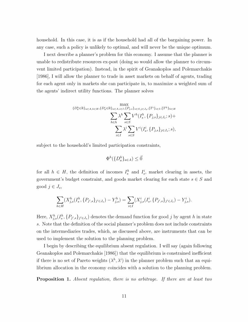
I next describe a planner’s problem for this economy. I assume that the planner is

unable to redistribute resources ex-post (doing so would allow the planner to circum-

vent limited participation). Instead, in the spirit of Geanakoplos and Polemarchakis

[1986], I will allow the planner to trade in asset markets on behalf of agents, trading

for each agent only in markets she can participate in, to maximize a weighted sum of

the agents’ indirect utility functions. The planner solves

max{Dh

a∈R}a∈A,h∈H ,{Dia∈R}a∈A,i∈I ,{Pj,s}s∈S,j∈Js ,{T i}i∈I ,{Th}h∈H∑

h∈h

λh∑s∈S

V h(Ihs , {Pj,s}j∈Js ; s)+∑i∈I

λi∑s∈S

V i(I is, {Pj,s}j∈Js ; s),

subject to the household’s limited participation constraints,

Φh({Dha}a∈A) ≤ ~0

for all h ∈ H, the definition of incomes Ihs and I is, market clearing in assets, the

government’s budget constraint, and goods market clearing for each state s ∈ S and

good j ∈ Js,∑h∈H

(Xhj,s(I

hs , {Pj′,s}j′∈Js)− Y h

j,s) =∑i∈I

(X ij,s(I

is, {Pj′,s}j′∈Js)− Y i

j,s).

Here, Xhj,s(I

hs , {Pj′,s}j′∈Js) denotes the demand function for good j by agent h in state

s. Note that the definition of the social planner’s problem does not include constraints

on the intermediaries trades, which, as discussed above, are instruments that can be

used to implement the solution to the planning problem.

I begin by describing the equilibrium absent regulation. I will say (again following

Geanakoplos and Polemarchakis [1986]) that the equilibrium is constrained inefficient

if there is no set of Pareto weights (λh, λi) in the planner problem such that an equi-

librium allocation in the economy coincides with a solution to the planning problem.

Proposition 1. Absent regulation, there is no arbitrage. If there are at least two

11

households who are limited participants, the allocation is generically constrained in-

efficient in the sense of Geanakoplos and Polemarchakis [1986].

Proof. See the appendix, ...

Absent regulation on intermediaries, there can be no arbitrage. If there are assets

a ∈ Ah and a′ ∈ AI with identical payoffs (Za,s = Za′,s for all s ∈ S), they are perfect

substitutes from the perspective of intermediaries, and therefore must have the same

prices (Qa = Qa′). Constrained inefficiency is not surprising, either; although limited

participation is not identical to incomplete markets, the same pecuniary externalities

that generate constrained inefficiency in incomplete markets (see Geanakoplos and

Polemarchakis [1986]) apply in the context of limited participation.

Proposition 1 establishes “generic” inefficiency. In this context, “generic” means

that if there is an economy, with no regulation and at least two limited participants,

that is constrained efficient (meaning the allocation coincides with a solution to a

planning planning problem), there is a slightly perturbed version of the economy

that will be constrained inefficient. The specific perturbation I use in the proof,

following Geanakoplos and Polemarchakis [1986] and Farhi and Werning [2016], is a

perturbation to the utility functions of the agents. In contrast, if there is a constrained

inefficient economy, it will generically not be possible to perturb it to reach constrained

efficiency. Speaking loosely, the set of economies that achieve constrained efficiency

absent regulation form a “measure zero” subset of the set of all economies.

I next turn to implementations of solutions to the social planning problem. I

will consider implementations of solutions to the planning problem that generate

constrained efficiency through regulation on the trades of intermediaries. The next

proposition shows that, generically, there exist regulations that simultaneously gen-

erate constrained efficiency and bring about arbitrage.

Proposition 2. For a given set of strictly positive Pareto weights, there exist regu-

lations {Φi}i∈I and an equilibrium given those regulations such that the equilibrium

allocation coincides with a solution to the planning problem with those Pareto weights.

Generically, in the set of strictly positive Pareto weights, there is arbitrage in this

equilibrium.

Proof. See the appendix, ...

12

Proposition 2 establishes that, for a given set of Pareto weights, it is possible for

a planner to implement the constrained efficient allocation via regulation. This is

not particularly surprising– all trade goes through intermediaries, and by regulating

those intermediaries, the planner can achieve any allocation, and in particular any

constrained efficient allocation. More surprising is the second part of the statement–

that, generically, the equilibrium features arbitrage. This arbitrage reflects the desire

of the planner to control the asset allocations of both households and intermediaries,

using regulations on the trades of intermediaries.

To summarize, this section shows that an absence of arbitrage does not imply

efficiency, and that efficiency does not imply an absence of arbitrage. Taken together,

these results suggest that arbitrage and efficiency are simply unrelated. This is not

the case; in the next section, I will show that, under the optimal regulatory regime,

the “pattern of arbitrage” across various states of the nature is closely related to the

notion of “wedges” that are typically used to analyze externalities. I will argue that,

but looking at the patterns of arbitrage across financial assets, regulators can asses

whether the regulations they implement are having their desired effects.

3 Arbitrage and Wedges

I begin this section by defining the “wedges,” τj,s, which are defined for each state

s ∈ S and good j ∈ Js. These wedges represent the difference between the first-order

conditions of the planner and of the agents– the latter do not take into account the

effects that their asset allocation decisions have on goods prices, and these pecuniary

externalities, due to limited participation, have welfare consequences. Let πs denote

an arbitrary full-support probability distribution over the states s ∈ S1, let πsµj,s

denote the multiplier, in the planner’s problem, on the market clearing constraint

of good j ∈ Js in state s ∈ S1, and let κ denote the planner’s multiplier on the

government budget constraint. Define the wedges τj,s using an orthogonal projection

of the multipliers on to prices:

µj,s = µsPj,s − κτj,sPj,s,

13

with∑

j∈Js τj,sPj,s = 0 for all s ∈ S.5

The multipliers µj,s represent the social marginal cost of demand for good j in

state s, and the multiplier κ is the social marginal value of resources at time zero.

To the extent that the multipliers µj,s are not proportional to prices (i.e. that the

τj,s are not zero), pecuniary externalities exist in the equilibrium. A high value of

the wedge τj,s indicates that the multiplier µj,s is low relative to the price Pj,s, which

is to say that the social marginal cost of demand for the good is less than the price.

Scaling the wedges τj,s by the multiplier κ ensures that the units of these wedges are

in “dollars,” rather than units of social utility.

These externalities can be compensated for by transferring income in state s to

household h from an intermediary i, if household h has a different marginal propensity

to demand good j in state s than the intermediary does. Transfers between households

with differing marginal propensities to demand could also accomplish the same goal

(transfers between intermediaries, who have the same homothetic utility function,

would have no effect). Let XhI,j,s denote the marginal effect that income has on the

demand of household h for good j in state s, holding prices constant. Let πs denote an

arbitrary probability distribution with full support over the state s ∈ S. If the wedge-

weighted difference of the income effects for the household and the intermediary,

∆h,is =

∑j∈Js

τj,sPj,s(XhI,j,s −X i

I,j,s),

is positive, transferring income from intermediary i to household h in state s has a

benefit, from the planner’s perspective, because it alleviates pecuniary externalities.

However, it might also have a cost, if the Pareto-weighted marginal utilities of income

between intermediary i and household h in state s are not equalized. For transfers

that are feasible (in the span of the assets tradeable by household h), under an optimal

policy, these costs and benefits will exactly offset. That is, in a constrained efficient

allocation, for all households h ∈ H, intermediaries i ∈ I, and assets a ∈ Ah,

∑s∈S

πs∆h,is Za,s =

∑s∈S

(V iI,s

V iI,s0

−V hI,s

V hI,s0

)Za,s, (1)

where V hI,s denotes the marginal value of income for household h in state s, and V i

I,s

5This definition of wedges is the same as the one employed by Farhi and Werning [2016], adjustedfor the differences between production and endowment economies.

14

is that object for intermediary i.

Put another way, we can view ∆h,is as the difference of two stochastic discount

factors– one for the household h and one for the intermediary. Each of these stochas-

tic discount factors reflects the ratio of the agent’s marginal utilities in state s and

state s0, adjusted for any differences between that agent’s beliefs and the measure

π. Neither of these SDFs can be used to price all assets, because of the limited par-

ticipation constraints (for households) and regulations (for intermediaries). However,

for particular assets (the assets in Ah for household h, the Arrow securities for an

intermediary) that are not affected by these constraints, the relevant SDF does in

fact price the asset. Consequently, the amount of arbitrage between an asset a ∈ Ah

and its replicating portfolio of Arrow securities in the intermediary market will also

be determined by the wedges. This result is stated below in 3.

I next elaborate on the importance of the assumption that the intermediaries

have identical, homothetic preferences. A direct consequence of this assumption is

that X iI,j,s = X i′

I,j,s for all i, i′ ∈ I, j ∈ Js, and s ∈ S. As a result, there is never

any particular reason to transfer wealth across intermediaries. It follows that it

is not necessary to regulate intermediaries’ trades in the Arrow securities market,

AI . I will focus on implementations of the constrained efficient allocations without

regulation of trade in the Arrow securities, primarily because these implementations

feature meaningful prices for the Arrow securities. An alternative implementation

that dictated all trades for intermediaries would not need to have asset prices at all,

and hence the question of the existence of arbitrage would be ill-defined.

However, this assumption has economic content. It implies that the social planner

is indifferent to the distribution of wealth across intermediaries. Put another way, the

regulator has “macro-prudential” motives for regulation, but not “micro-prudential”

motives. In section §6, I discuss how micro-prudential motives for regulation might

change the interpretation of my results.

I now present the main result of this section: the relationship between the wedges

(as summarized by the differences ∆) and arbitrage, in a constrained efficient alloca-

tion implemented without regulation of the Arrow securities market.

Proposition 3. Consider a constrained efficient allocation implemented by regula-

tions {Φi}i∈I that do not regulate trade in the Arrow securities AI . For any security

15

tradeable by household h (a ∈ Ah), define the amount of arbitrage as

χa = −Qa +∑s∈S

Za,sQs,

where Qa is the price of the asset and Qs is the price of an Arrow security paying off

in state s.

Then, for any intermediary i ∈ I,

χa =∑s∈S

πs∆h,is Za,s.

Proof. See the appendix, ...

In words, an asset tradeable by households will be cheap, relative to its Arrow-

market replicating portfolio, if its payoffs occur mainly in states for which the planner

would like to transfer wealth from intermediaries to households.

As a special case, consider a risk-free asset (Za,s = 1 for all s 6= s0, recalling

that Za,s0 = 0 by convention), and suppose that there are two goods, “houses” and

“yachts,” bought exclusively by households and intermediaries, respectively. If there

are positive externalities in demand for houses in the future, and/or negative exter-

nalities in demand for yachts, (τhouses,s < 0 and τyachts,s > 0), then it will alleviate

externalities to transfer wealth to households in the future (∆h,is > 0). As a result, in

equilibrium, the risk-free asset available to households will have a lower price (higher

interest rate) than the risk-free asset available to intermediaries.

In the next section, I invert this exercise: given an observed pattern of arbitrage,

what can we say about ∆h,is ? That is, presuming regulation is optimal, in which states

must the regulator believe there are externalities that justify transferring wealth from

intermediaries to households or vice versa?

4 The Externality-Mimicking Portfolio

Suppose a financial economist observes, in financial markets, a set of securities Aarb

that she believes are tradable by households and for which the financial economist

also observes a replicating portfolio of securities traded only by intermediaries (e.g.

derivatives). I will call these assets “arbitrageable,” meaning that, if the prices of

16

these securities were not consistent with the prices of their replicating portfolio, there

would be arbitrage. Many securities will not be arbitrageable, from the perspective

of the financial economist, because she does not observe the price of the replicating

portfolio of derivatives.

For each arbitrageable security a ∈ Aarb, by observing the price of the security

and of the replicating portfolio of derivatives, the financial economist can compute

the amount of arbitrage, χa. Examples of this sort of exercise include the covered

interest parity violations documented by Du et al. [2017], the arbitrage between asset-

swapped TIPS and treasury bonds documented by Fleckenstein et al. [2014], and the

basis between corporate bonds and credit default swaps discussed in Garleanu and

Pedersen [2011].

To varying degrees, each of these “arbitrages” is not exactly a textbook arbitrage.

One can always imagine stories (e.g. jumps to default by derivatives counterparties

correlated with the value of the derivative contract) that could justify small pricing

deviations. I view these issues as quantitatively insignificant (in most of the cases

cited above), and for the purposes of discussion will assume that each of these authors

has in fact documented an arbitrage. The “cleanest” arbitrage of all is perhaps the

ability of banks in the US to borrow overnight from the GSEs in the fed funds market

and earn interest on excess reserves (Bech and Klee [2011]). Because this arbitrage

has only an overnight maturity, and there is no counterparty risk, it is very difficult

to come up with a story, aside from regulation, to explain why banks would not be

willing to engage in the arbitrage.

Suppose we observed these arbitrages, and we assume that the equation of 3 holds:

for each a ∈ Aarb,χa =

∑s∈S

πs∆h,is Za,s,

for any household h ∈ H that can trade the security a ∈ Aarb. If the set Aarb contained

a full set of Arrow securities (or was a complete asset market, more generally), there

would be a one-to-one mapping between the arbitrage on these securities and the

differences ∆h,is (under a fixed probability distribution πs). Empirically, although

there are multiple examples of assets with arbitrage, it would be a stretch to say that

the financial economist observes a complete market in arbitrageable securities.6 As a

6The existence of a full set of Arrow securities in Aarb is (at least in theory) consistent withthe assumption of limited participation. To be in Aarb, some household must be able to trade thesecurity, but these does not imply that every household can trade the security.

17

result, it will not be possible, empirically, to recover ∆h,is for all states s ∈ S.

We can, however, attempt to project the differences ∆h,is on to a lower-dimensional

space, and require that this projection be consistent with the amount of arbitrage we

observe in data. This procedure, which I will describe next, builds on ideas introduced

by Hansen and Richard [1987]. There are essentially two ways to look at the procedure

I employ. The first is that I am simply projecting the differences ∆h,is on to the space

of asset returns, perhaps after employing a non-linear transformation. The second is

that I am attempting to make the risk-neutral measures for the intermediaries and for

households as similar as possible. I will begin by describing this second perspective,

and then demonstrate in lemma 1 that they are equivalent.

I will assume that the set Aarb includes a risk-free security, and I will define the

risk-free interest rate for intermediaries, Ri, as

Ri = (∑s∈S1

V iI,s

V iI,s0

)−1,

and define another risk-free interest rate Rh in similar fashion. If there is arbitrage on

risk-free securities, these two interest rates will not be equal, and are both observable

in data. Using these interest rates, I define a risk-neutral measure for intermediaries,

πis = RiV iI,s

V iI,s0

,

and define πhs along similar lines.

Hansen and Richard [1987] study the problem of minimizing the variance of a

stochastic discount factor, subject to the constraint that the SDF price a set of

assets. Sandulescu et al. [2017] study a generalized version of this problem, minimizing

some moment (not necessarily the variance) of the SDF. An SDF is, of course, also

the Radon-Nikodym derivative between two measures– in these applications, a risk-

neutral measure and the physical measure. The problem of Hansen and Richard [1987]

(and of Sandulescu et al. [2017] more generally) can be recast as minimizing the value

of a divergence between the risk-neutral measure and the physical measure, subject

to the constraint that the risk-neutral measure correctly price assets. The particular

divergence that corresponds to the variance minimization procedure of Hansen and

18

Richard [1987] is the “chi-squared” divergence,7

Dχ2(π||π′) =1

2

∑s∈S1

π′

s(πsπ′s− 1)2.

These procedures have the virtue that they make the estimated risk-neutral mea-

sure as “close” as possible to the physical measure, under a definition of “close”

defined by the divergence in question. In this context of this paper, I could apply

this procedure to both the measure associated with intermediaries (πis) and the mea-

sure associated with households (πhs ), making each of them as close as possible to

the physical measure. However, this requires an econometric exercise (estimating the

moments of returns under the physical measure) and will not necessarily minimize

the estimated amount of arbitrage. That is, by making the households’ and interme-

diaries’ measures as close as possible to the physical measure, we do not necessarily

make them as close as possible to each other.

Instead, I will minimize the value of the chi-squared divergence between the house-

holds’ measure, πh, and the intermediaries’ measure, πi, subject to the constraint that

the observed price of the asset for households is correct. That is, letting P(S) denote

the simplex over time-one states, I solve

πh = minπ∈P(S)

Dχ2(π||πi)

subject to, for each a ∈ Aarb,

(Rh)−1∑s∈S1

πsZa,s + χa = (Ri)−1∑s∈S1

πisZa,s.

This procedure has two virtues. First, it minimizes arbitrage, as measured by the

divergence between the two risk-neutral probability measures. Second, we will see

that the estimated measure πh is entirely a function of the moments of asset payoffs

under the risk-neutral measure of intermediaries.8 Consequently, if we observe a

7The general definition of a divergence D(π′||π) is a weakly positive scalar function of two prob-ability measures that is zero if and only if π′ = π. The more general procedure of Sandulescu et al.[2017] minimizes an α-divergence, which is a particular family of divergences that includes the χ2

divergence.8The procedure also has a disadvantage, which is that πh might not have full support. For

discussions of this issue, see Hansen and Richard [1987] and Hansen and Jagannathan [1991]. Usingan alternative divergence, such as the Kullback-Leibler divergence, as in Sandulescu et al. [2017],

19

sufficiently rich set of asset prices traded only by intermediaries, we can construct

πh from those asset prices, without any econometrics. In the next section, I will use

options prices on currency pairs to put this idea into practice.

One additional complication is that (at least in theory) there might not be a single

household h∗ that can trade all the assets in Aarb. I will ignore this issue, and assume

that such a household does exist. Additionally, it is convenient to work in the space

of returns, rather than payoffs. For this reason, I will assume that the payoff of each

asset in Aarb is weakly positive in all states of the world.

As noted above, the differences ∆h∗,is are defined with respect to a probability

measure. I will work with the particular differences defined with respect to the

intermediaries’ risk-neutral probability measure, πi, and call these differences the

“risk-neutral externalities.” From an estimated risk-neutral measure πh and the risk-

neutral measure πi, we can construct an estimated set of risk-neutral externalities,

∆h∗,is . Defining χR = 1

Ri − 1Rh as the arbitrage on the risk-free asset, we can define

the estimated risk-neutral externalities as (consistent with equation (1))

∆h∗,is = χR +

1

Rh(1− πhs

πis). (2)

An alternative approach would simply be to project (in the least squares sense)

the risk-neutral externalities on to the space of returns. Define the excess returns for

intermediaries as

Ria,s = Ri Za,s∑

s′∈S1πis′Za,s′

−Ri,

and let Aarb \ {aRF} denote the set of arbitrageable assets excluding the risk-free

assets. Let Σi be the covariance matrix of returns for risky assets in Aarb under the

risk-neutral measure πi. Given these definitions, the least squares projection is

∆h∗,is = χR +Ri

∑a,a′∈Aarb\{aRF }

(χa∑

s′∈S1πis′Za,s′

− χR)(Σi)−1a,a′Ria′,s.

The following lemma shows that the least squares projection (∆h∗,is ) is identical to

the estimate of the risk-neutral externalities that minimizes the chi-squared divergence

between the household and intermediaries’ risk-neutral measures (∆h∗,is ).

would remove this problem, but would break the equivalence between the divergence minimizationand least squares projection.

20

Lemma 1. Let πh be the measure for that minimizes the chi-squared divergence be-

tween itself and the intermediaries’ risk-neutral measure, subject to the constraint that

πh correctly price each asset in Aarb from the households’ perspective:

πh = minπ∈P(S)

Dχ2(π||πi)

subject to, for each a ∈ Aarb,

(Rh)−1∑s∈S1

πsZa,s + χa = (Ri)−1∑s∈S1

πisZa,s.

If the measure πh has full support, then the associated estimate of the risk-neutral

externalities, ∆h∗,is = χR + 1

Rh (1 − πh

πi ), is equal to the least-squares projection of the

externalities on to the space of returns, ∆h∗,is .

Proof. See the appendix, section C.2.

This lemma can also be understood in terms of a portfolio problem. The portfolio

weights

θ∗a′ =∑

a∈Aarb\{aRF }

Ri(χa∑

s′∈S1πis′Za,s′

− χR)(Σi)−1a,a′ , (3)

plus some amount of the risk-free asset, form a zero-cost portfolio whose returns

are the unexpected component of ∆h∗,is . I will call this portfolio the “risk-neutral

externality-mimicking portfolio.” The caveat in lemma 1, which I will ignore in what

follows, applies to situations when the risk-neutral externality-mimicking portfolio

has a gross return of less than negative one, breaking limited liability. This could

occur if the portfolio is “short” one of the assets, but is very unlikely for the types of

assets and time horizons that I study.

The risk-neutral externality-mimicking portfolio is the portfolio of assets that

is the unique projection of the planner’s perceived externalities on to the space of

available payoffs, given the intermediaries’ risk-neutral measure πi. In other words, its

return is the best linear approximation of the conditional expectation of ∆h∗,is given

the returns of the arbitrageable assets. In this sense, when its return is high, the

planner must generally think that it would alleviate externalities to transfer wealth

from intermediaries to households, and when its payoff is low, the planner must

generally think it would alleviate externalities to transfer wealth to intermediaries

21

from households.

Continuing the analogy with the procedure of Hansen and Richard [1987], I discuss

a bound along the lines of Hansen and Jagannathan [1991]. In this analogy, as

above, the intermediaries’ measure πis will play the role of the physical measure, and

the households measure πhs will play the role of the risk-neutral measure. As in

the latter paper, the standard deviation (under the measure πis) of any “stochastic

discount factor” πhs

Rhπis, divided by its mean (also under πis) must be greater than the

corresponding statistic for the least-squares projection, πhs

Rhπis. Moreover, for the least

squares projection, this statistic is also equal to the “arbitrage Sharpe ratio” of the

portfolio θ∗a. I define the “arbitrage Sharpe ratio” for any portfolio θ as

Si(θ) =|∑

a∈Aarb θaRi( χa∑

s′∈S1πis′Za,s′

− χR)|

σi(∑

a∈Aarb θaRia,s)

,

where σi(·) denotes the standard deviation under the measure πi. The numerator

is the expected excess return (under the intermediaries’ risk-neutral measure) due

to arbitrage available to intermediaries that purchase assets available to households.

That is, it is not the entire expected excess return, as in the usual definition of the

Sharpe ratio, but only the portion due to “excess arbitrage,” meaning arbitrage in

excess of the arbitrage available on the risk-free asset.

The analogy to the bound of Hansen and Jagannathan [1991] is described in the

following lemma.

Lemma 2. For any risk-neutral externalities ∆h,is that satisfying the arbitrage pricing

equation of 3, and any portfolio θ,

Rhσi(∆h,is ) ≥ Rhσi(∆h,i

s ) = Si(θ∗) ≥ Si(θ).

Proof. See the appendix, section C.3.

This lemma provides an alternative perspective on the least squares projection

procedure. One can view the projection procedure (or, equivalently, the divergence

minimization procedure) as searching for a portfolio with the highest arbitrage Sharpe

ratio. It also shows that the arbitrage Sharpe ratio of any portfolio places a lower

bound on the volatility of the risk-neutral externalities, and the tightest possible

bound is formed using the externality-mimicking portfolio.

22

The externality-mimicking portfolio is a reflection of what regulation is actually

accomplishing. We can compare it to the stated objectives of regulators, and in

particular to the “stress tests” conducted by the Federal Reserve and other central

banks. These “stress test” scenarios presumably reflect situations in which the Federal

Reserve would like intermediaries to have more wealth than the intermediaries would

choose to have on their own, indicating some perception of externalities.

For example, the 2017 Stress Test Scenarios9 involve, in the “severely adverse”

scenario, a depreciation of the euro and pound, and an appreciation of the yen,

relative to the US dollar. Du et al. [2017] document that CIP violations with a

common pattern across these currencies: investing in euros, pounds, or yen bonds,

and using a forward contract to swap back to dollars, offers a higher return than

investing in dollars, at the beginning of 2017. This suggests something inconsistent:

the externality-mimicking portfolio treats euro, pounds, and yen roughly equally, but

the stress test scenario treats them differently. In this next section, I explore this idea

in more detail.

5 Empirical Estimates

In this section, I estimate externality-mimicking portfolios and study the returns

that the portfolios would experience in the “stress tests” conducted by the federal

reserve. Constructing these portfolios requires, for each asset price that we as fi-

nancial economists observe, taking a stand on whether that asset price comes from

the intermediaries-only market or from a market in which both intermediaries and

households can participate. Reality, of course, is more complicated; for example,

some assets are rarely owned by individuals, but held by many money-market funds

or mutual funds, and for our purposes might be thought of as tradable by households.

These abstract difficulties are often easier to resolve in the context of specific

arbitrages. The empirical application I consider features two arbitrages: an arbitrage

between household interest rates and the interest on excess reserves (IOER), and

covered interest parity violations. The horizon of the arbitrage I study is one month.

The first arbitrage involves the yield difference of two (essentially) risk-free assets.

A bank can earn interest on excess reserves held at the Federal Reserve. If there is no

meeting of the FOMC within the next month, the bank is essentially guaranteed to

9https://www.federalreserve.gov/newsevents/pressreleases/files/bcreg20170203a5.pdf

23

earn one month’s worth of interest at the current overnight rate. Of course, in rare

circumstances, the Federal reserve might choose to change the interest on reserves

between meetings, but such changes have low ex-ante likelihood and are unlikely to

materially alter the expected interest rate.

A household, in contrast, cannot earn the rate of interest on excess reserves.

As an alternative, it could invest in treasury bills, highly-rated commercial paper,

repo agreements (via money market funds), bank deposits, or the like. There is a

significant literature arguing that treasury bonds are special, relative to other bonds

the would appear to be close substitutes (e.g. Fleckenstein et al. [2014]), perhaps

due to their additional liquidity or some other kind of benefits. I will use 1-month

OIS swap rates, which closely track the yields of one-month maturity highly-rated

commercial paper in the US, as a proxy for a risk-free rate available to households

that provides no liquidity benefits. These rates tend to be higher than the rates

on one-month constant maturity treasuries, but lower than LIBOR rates (which may

include credit risk). For example, on August 19th, 2016 (a little over one month before

the next FOMC meeting), 1 month constant-maturity treasury rates were 27bps, AA

non-financial one-month commercial paper rates were 37bp, one-month OIS swaps

were 40bps, the interest on excess reserve rates were 50bps, and one month LIBOR

was 52bps. In the notation of the previous section, the annualized household risk

free return (Rh)12 is 1.004 and the annualized intermediary risk-free return (Ri)12 is

1.005.

The next arbitrage is a covered interest parity violation. I will assume that house-

holds can purchase euros with dollars, and invest their euros at the 1-month OIS

swap rate in euros (the EONIA rate). What households cannot do (but intermedi-

aries can) is trade currency forwards. The intermediary can replicate the household’s

euro/EONIA trade by investing dollars at the IOER rate, and selling dollars for eu-

ros using a 1-month currency forward. The households can invest in euros/EONIA

instead of investing their dollars at the 1-month OIS swap rate in dollars, and hence

the difference between these two strategies is also an asset in their payoff space.

That is, one could either define the arbitrage as being about zero-cost portfolios

(the difference in these two strategies vs. the forward), or using positive-cost strategies

(investing in euros/EONIA vs. the bank investing at IOER and using the forward).

However, these two alternatives are simply linear rotations of the payoff Zs and the

arbitrages χ, and hence will yield identical estimates of ∆h∗,is . The first strategy is

24

analogous to the approach of Du et al. [2017], but the latter has the benefit that the

portfolio problem can be implemented in the space of returns rather than payoffs. For

this reason, in what follows, I will pursue the latter approach and consider arbitrages

between positive-cost strategies.

In my empirical exercise, I will consider portfolios of the risk-free arbitrage and

investments in euros and yen, and use an investments in pounds as a sort of “out-

of-sample” test. To estimate the risk-neutral externality mimicking portfolio, it is

sufficient to estimate the arbitrage on the risk-free assets and each of the risky assets,

along with the covariance matrix of the risky assets under the intermediaries’ risk-

neutral measure. Estimates of the arbitrage can be constructed from spot and forward

currency rates, the IOER rate, and OIS swap rates, as in Du et al. [2017]. Estimates of

the risk-neutral covariance matrix between various currency pairs can be constructed

from options on exchange rates. In particular, the availability of dollar-euro, dollar-

pound, dollar-yen, euro-yen, euro-pound, and pound-yen options allows me to extract

an entire risk-neutral variance-covariance matrix from options prices. I assume that

the at-the-money FX options prices I observe come from the intermediary-only market

(and hence the IOER rate is the appropriate discount rate), and that the distribution

of future exchange rates is log-normal. The formula of Black [1976] applies, and

using this formula I extract risk-neutral variances and covariances. More elaborate

constructions, using out-of-the-money options as in the construction of the VIX index,

are possible and would dispense with the need to assume log-normality, at the expense

of additional complexity.

This procedure can be run at daily frequency, for all dates at least one month

before a scheduled FOMC meeting. I will begin by presenting summary statistics

for the magnitude of the arbitrage in question. The dataset consists of daily data

from financial markets between January 2011 and September 2016, including only

those dates that are at least one month (more than 23 non-weekend days) before

the start of the next scheduled FOMC meeting and not meeting dates themselves.

Because the FOMC holds eight scheduled meetings each year, roughly one quarter of

all non-weekend days are included in the dataset.

The first summary statistics I will present contain the sample means and standard

deviations of the arbitrage associated with each currency, as well as the risk-free

25

arbitrage. Conceptually, these statistics correspond to the term

χa =−Qa +

∑s∈S Za,sQs∑

s∈S Za,sQs

.

For example, for euros, it represents the percentage difference in price, in dollars

today, of purchasing a single euro one month in the future by buying the euro at spot

today and saving at OIS (households, Qa), and obtaining the same euro one month in

the future by savings at the IOER rate and using a currency forward (intermediaries,∑s∈S Za,sQs). I also present the difference in dollar zero-coupon bonds prices, scaled

by the interest rate for intermediaries (RiχR), which is a function of the difference

between the dollar OIS rate and the IOER rate.

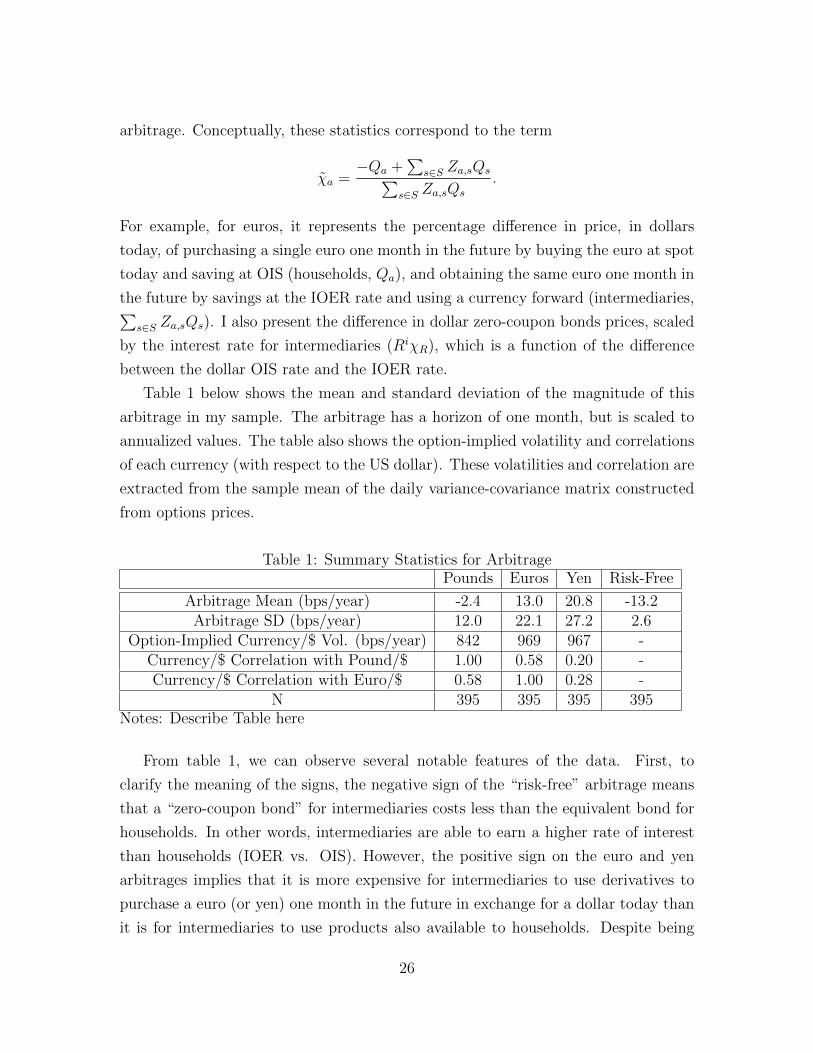
Table 1 below shows the mean and standard deviation of the magnitude of this

arbitrage in my sample. The arbitrage has a horizon of one month, but is scaled to

annualized values. The table also shows the option-implied volatility and correlations

of each currency (with respect to the US dollar). These volatilities and correlation are

extracted from the sample mean of the daily variance-covariance matrix constructed

from options prices.

Table 1: Summary Statistics for ArbitragePounds Euros Yen Risk-Free

Arbitrage Mean (bps/year) -2.4 13.0 20.8 -13.2Arbitrage SD (bps/year) 12.0 22.1 27.2 2.6

Option-Implied Currency/$ Vol. (bps/year) 842 969 967 -Currency/$ Correlation with Pound/$ 1.00 0.58 0.20 -Currency/$ Correlation with Euro/$ 0.58 1.00 0.28 -

N 395 395 395 395Notes: Describe Table here

From table 1, we can observe several notable features of the data. First, to

clarify the meaning of the signs, the negative sign of the “risk-free” arbitrage means

that a “zero-coupon bond” for intermediaries costs less than the equivalent bond for

households. In other words, intermediaries are able to earn a higher rate of interest

than households (IOER vs. OIS). However, the positive sign on the euro and yen

arbitrages implies that it is more expensive for intermediaries to use derivatives to

purchase a euro (or yen) one month in the future in exchange for a dollar today than

it is for intermediaries to use products also available to households. Despite being

26

able to save at the IOER rate instead of the USD OIS rate, the magnitude of the

covered interest parity (CIP) violation more than offsets this effect. Of course, this is

not necessarily “bad news” for intermediaries– it simply means that inter. However,

for pounds, these two effects roughly offset (on average). That is, the extra interest an

intermediary can earn by saving at the IOER rate is roughly offset by the magnitude

of the pound-dollar CIP violation. Finally, note that, at least for euros and yen,

the covariance matrix of currency returns is reasonably close to a scaled version of

the identity matrix. As a result, the portfolio weights constructed as in equation (3)

above will be roughly proportional to the amount of “excess arbitrage,” χa − RiχR,

observed for each asset.

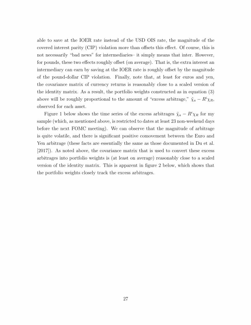
Figure 1 below shows the time series of the excess arbitrages χa − RiχR for my

sample (which, as mentioned above, is restricted to dates at least 23 non-weekend days

before the next FOMC meeting). We can observe that the magnitude of arbitrage

is quite volatile, and there is significant positive comovement between the Euro and

Yen arbitrage (these facts are essentially the same as those documented in Du et al.

[2017]). As noted above, the covariance matrix that is used to convert these excess

arbitrages into portfolio weights is (at least on average) reasonably close to a scaled

version of the identity matrix. This is apparent in figure 2 below, which shows that

the portfolio weights closely track the excess arbitrages.

27

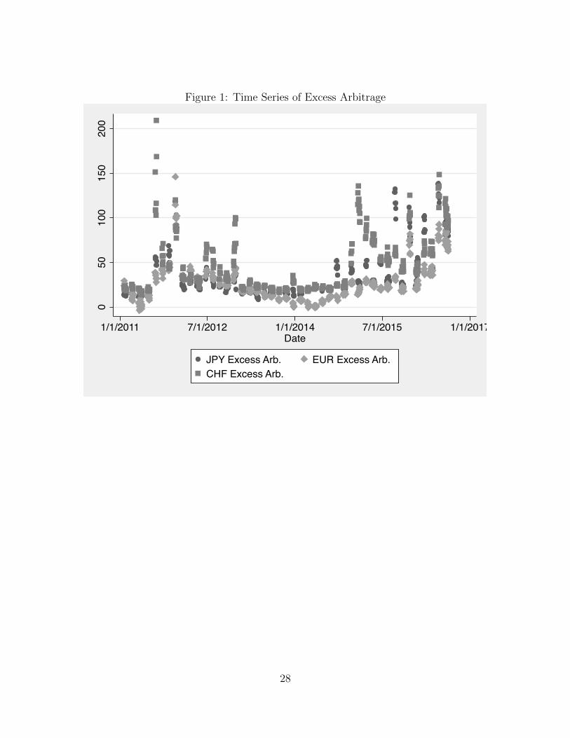
Figure 1: Time Series of Excess Arbitrage0

5010

015

020

0

1/1/2011 7/1/2012 1/1/2014 7/1/2015 1/1/2017Date

JPY Excess Arb. EUR Excess Arb.CHF Excess Arb.

28

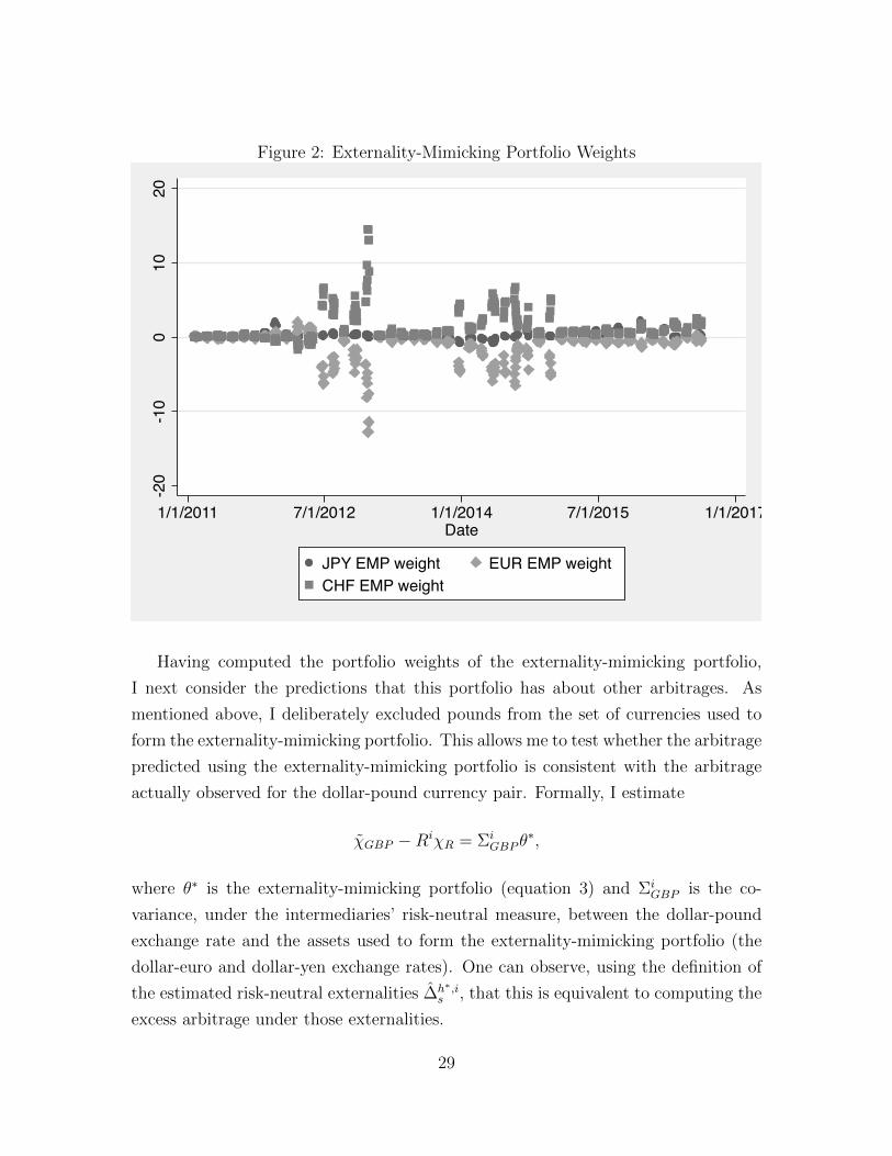
Figure 2: Externality-Mimicking Portfolio Weights-2

0-1

00

1020

1/1/2011 7/1/2012 1/1/2014 7/1/2015 1/1/2017Date

JPY EMP weight EUR EMP weightCHF EMP weight

Having computed the portfolio weights of the externality-mimicking portfolio,

I next consider the predictions that this portfolio has about other arbitrages. As

mentioned above, I deliberately excluded pounds from the set of currencies used to

form the externality-mimicking portfolio. This allows me to test whether the arbitrage

predicted using the externality-mimicking portfolio is consistent with the arbitrage

actually observed for the dollar-pound currency pair. Formally, I estimate

χGBP −RiχR = ΣiGBP θ

∗,

where θ∗ is the externality-mimicking portfolio (equation 3) and ΣiGBP is the co-

variance, under the intermediaries’ risk-neutral measure, between the dollar-pound

exchange rate and the assets used to form the externality-mimicking portfolio (the

dollar-euro and dollar-yen exchange rates). One can observe, using the definition of

the estimated risk-neutral externalities ∆h∗,is , that this is equivalent to computing the

excess arbitrage under those externalities.

29

Figure 3 displays the results graphically. The actual excess arbitrage in pounds is

constructed from OIS rates in dollars and pounds, and the spot and forward dollar-

pound exchange rates (using excess arbitrage eliminates the dependence on the IOER

rate). The predicted excess arbitrage is constructed entirely from those same variables

in euros and yen, along with options prices on all six possible currency pairs, which

are used to both construct the externality mimicking portfolio (in the matrix Σi) and

to construct the covariances ΣiGBP . In other words, the set of financial instruments

used to construct the actual and predicted excess arbitrages do not overlap at all.

Nevertheless, the predicted and actual excess arbitrages closely track each other.

Regressing the actual excess arbitrage on the predicted excess arbitrage, without

a constant, results in an R2 of 74%. This suggests that the mimicking portfolio

constructed from euros and yen tracks the unobservable risk-neutral externalities

reasonably well (or at least that adding pounds does not improve things much).

Figure 3: Actual vs. Predicted Excess Arbitrage in Pounds

050

100

1/1/2011 7/1/2012 1/1/2014 7/1/2015 1/1/2017Date

GBP Excess Arb. Predicted GBP Excess Arb.

I now turn to the question of what the estimates of the externality-mimicking

30

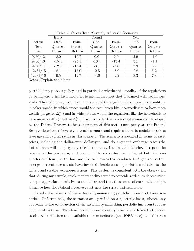
Table 2: Stress Test “Severely Adverse” ScenariosEuro Pound Yen

StressTestDate

One-QuarterReturn

Four-QuarterReturn

One-QuarterReturn

Four-QuarterReturn

One-QuarterReturn

Four-QuarterReturn

9/30/12 -8.0 -16.7 0.0 0.0 2.9 -1.09/30/13 -15.4 -24.1 -13.4 -13.4 3.1 -1.19/30/14 -12.7 -14.4 -3.1 -3.6 7.9 6.712/31/15 -8.1 -15.0 -2.5 -3.9 2.8 5.212/31/16 -9.5 -12.7 -4.6 -9.2 3.3 7.8

Notes: Explain table here

portfolio imply about policy, and in particular whether the totality of the regulations

on banks and other intermediaries is having an effect that is aligned with regulators’

goals. This, of course, requires some notion of the regulators’ perceived externalities;

in other words, in which states would the regulators like intermediaries to have more

wealth (negative ∆h,is ) and in which states would the regulators like the households to

have more wealth (positive ∆h,is ). I will consider the “stress test scenarios” developed

by the Federal Reserve to be a statement of this sort. Once per year, the Federal

Reserve describes a “severely adverse” scenario and requires banks to maintain various

leverage and capital ratios in this scenario. The scenario is specified in terms of asset

prices, including the dollar-euro, dollar-yen, and dollar-pound exchange rates (the

last of these will not play any role in the analysis). In table 2 below, I report the

returns of the yen, euro, and pound in the stress test scenarios, at both the one

quarter and four quarter horizons, for each stress test conducted. A general pattern

emerges: recent stress tests have involved sizable euro depreciations relative to the

dollar, and sizable yen appreciations. This pattern is consistent with the observation

that, during my sample, stock market declines tend to coincide with euro depreciation

and yen appreciation relative to the dollar, and that these sorts of correlations might

influence how the Federal Reserve constructs the stress test scenarios.

I study the returns of the externality-mimicking portfolio in each of these sce-

narios. Unfortunately, the scenarios are specified on a quarterly basis, whereas my

approach to the construction of the externality-mimicking portfolio has been to focus

on monthly returns. The choice to emphasize monthly returns was driven by the need

to observe a risk-free rate available to intermediaries (the IOER rate), and this rate

31

is available at a daily frequency and (with very high probability) changes only on

FOMC meetings dates. In what follows, I will present the returns of the one-month

externality mimicking portfolio, pretending that the currency returns of the stress

test scenario at either the one quarter or four quarter horizons in fact occur over a

single month.

Each of the stress test scenarios is associated with a particular date (listed in

table 2) which is the date at which the scenario starts. For each date in my sample

(at least 23 non-weekend days before the next FOMC meeting) that is also within 180

calendar days of the stress test date, I report the returns of the externality-mimicking

portfolio constructed from that day’s interest rates, spot and forward exchange rates,

and exchange rate options under the associated stress test scenario. Requiring that

the relevant financial market data come from a day that is within 180 days of the

stress test date effectively assigns almost all of the days in my sample to a single

stress test date, dropping a handful of days that are far from any stress test date.

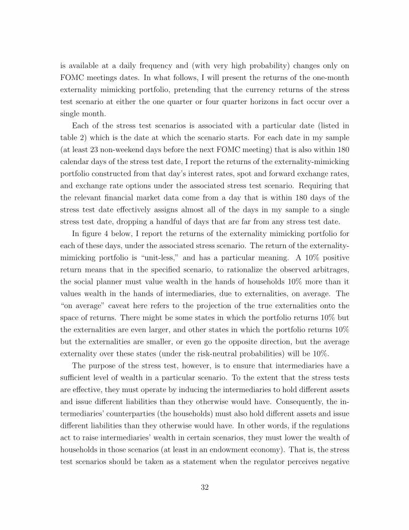
In figure 4 below, I report the returns of the externality mimicking portfolio for

each of these days, under the associated stress scenario. The return of the externality-

mimicking portfolio is “unit-less,” and has a particular meaning. A 10% positive

return means that in the specified scenario, to rationalize the observed arbitrages,

the social planner must value wealth in the hands of households 10% more than it

values wealth in the hands of intermediaries, due to externalities, on average. The

“on average” caveat here refers to the projection of the true externalities onto the

space of returns. There might be some states in which the portfolio returns 10% but

the externalities are even larger, and other states in which the portfolio returns 10%

but the externalities are smaller, or even go the opposite direction, but the average

externality over these states (under the risk-neutral probabilities) will be 10%.

The purpose of the stress test, however, is to ensure that intermediaries have a

sufficient level of wealth in a particular scenario. To the extent that the stress tests

are effective, they must operate by inducing the intermediaries to hold different assets

and issue different liabilities than they otherwise would have. Consequently, the in-

termediaries’ counterparties (the households) must also hold different assets and issue

different liabilities than they otherwise would have. In other words, if the regulations

act to raise intermediaries’ wealth in certain scenarios, they must lower the wealth of

households in those scenarios (at least in an endowment economy). That is, the stress

test scenarios should be taken as a statement when the regulator perceives negative

32

externalities associated with transferring wealth from intermediaries to households

(negative ∆h,is ). Consequently, we would expect, if the regulations were having the

desired effect, that the return on the externality mimicking portfolio in the stress test

scenario would be sharply negative.

What I find in the data, however, is that this is not the case. In both 2014 and

2015, the arbitrage on yen was larger than the arbitrage on euros (figure 1), and as

a result the externality mimicking portfolio placed more weight on yen than euros

(figure 2). The yen appreciation in the stress test scenario was large enough, given

this extra weight, to more than offset the euro depreciation, and as a result the return

on the externality mimicking portfolio was positive. In other words, even though the

Federal Reserve would like the intermediaries to have more wealth in the stress test

scenario, the cumulative effect of all regulations (by the Fed and other entities) acted

to encourage the banks to have less wealth in the stress test scenario. The situation

was better for the 2012 and 2013 stress tests, and appears better at the end of the

data for the 2016 test, mainly due to a higher weight on euros in the portfolio, which is

caused by an increase in the magnitude of the euro CIP violation. Note the surprising

logic of this statement: an increase in the magnitude of arbitrage can be understood

as a sign that regulation is working more effectively. To aid the comparison between

arbitrages, portfolio weights, and portfolio returns in the stress scenarios, section §Ain the appendix shows each of these on the same axis (days relative to the stress test

date), separately for each of the stress tests.

33

Figure 4: Externality Mimicking Portfolio Returns in Stress Scenarios0

5010

015

00

5010

015

0

-200 -100 0 100 200

-200 -100 0 100 200 -200 -100 0 100 200

30sep2012 30sep2013 30sep2014

31dec2015 31dec2016

One-Quarter EMP Stress Return Four-Quarter EMP Stress Return

days

Graphs by Stress Test Date

At first glance, the results for 2014 and 2015 seem like a contradiction. If the stress

test requires intermediaries to have more wealth when the euro depreciates and the

yen appreciates, shouldn’t this have an effect on intermediaries’ willingness to own

euros and yen, and hence be reflected in market prices? How can we reconcile the fact

that the stress test goes in “opposite directions” for euro and yen, but the arbitrages

we observe go in the “same direction”? Although I cannot provide a definitive answer

to this question, I will sketch a “story” that can explain these results. To explain

the existence of arbitrage, it must be the case that households (and institutions

like mutual funds that act on their behalf) are unable to execute the arbitrage, or

face prohibitively high costs, and the evidence of Rime et al. [2017] supports this

hypothesis. At the same time, there must be constraints on banks that raise the cost of

conducting the arbitrage. Leverage constraints, such as the “supplementary leverage

ratio,” described in D’Hulster [2009], have been suggested by Du et al. [2017] as a

relevant constraint, and are perhaps the only plausible interpretation of the IOER-

34

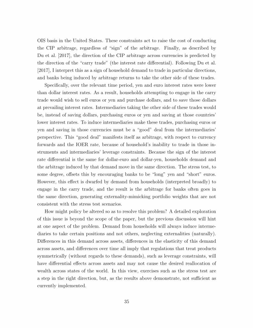
OIS basis in the United States. These constraints act to raise the cost of conducting

the CIP arbitrage, regardless of “sign” of the arbitrage. Finally, as described by

Du et al. [2017], the direction of the CIP arbitrage across currencies is predicted by

the direction of the “carry trade” (the interest rate differential). Following Du et al.

[2017], I interpret this as a sign of household demand to trade in particular directions,

and banks being induced by arbitrage returns to take the other side of these trades.

Specifically, over the relevant time period, yen and euro interest rates were lower

than dollar interest rates. As a result, households attempting to engage in the carry

trade would wish to sell euros or yen and purchase dollars, and to save those dollars

at prevailing interest rates. Intermediaries taking the other side of these trades would

be, instead of saving dollars, purchasing euros or yen and saving at those countries’

lower interest rates. To induce intermediaries make these trades, purchasing euros or

yen and saving in those currencies must be a “good” deal from the intermediaries’

perspective. This “good deal” manifests itself as arbitrage, with respect to currency

forwards and the IOER rate, because of household’s inability to trade in those in-

struments and intermediaries’ leverage constraints. Because the sign of the interest

rate differential is the same for dollar-euro and dollar-yen, households demand and

the arbitrage induced by that demand move in the same direction. The stress test, to

some degree, offsets this by encouraging banks to be “long” yen and “short” euros.

However, this effect is dwarfed by demand from households (interpreted broadly) to

engage in the carry trade, and the result is the arbitrage for banks often goes in

the same direction, generating externality-mimicking portfolio weights that are not

consistent with the stress test scenarios.

How might policy be altered so as to resolve this problem? A detailed exploration

of this issue is beyond the scope of the paper, but the previous discussion will hint

at one aspect of the problem. Demand from households will always induce interme-

diaries to take certain positions and not others, neglecting externalities (naturally).

Differences in this demand across assets, differences in the elasticity of this demand

across assets, and differences over time all imply that regulations that treat products

symmetrically (without regards to these demands), such as leverage constraints, will

have differential effects across assets and may not cause the desired reallocation of

wealth across states of the world. In this view, exercises such as the stress test are

a step in the right direction, but, as the results above demonstrate, not sufficient as

currently implemented.

35

6 Extensions

6.1 Micro-Prudential Motives for Regulation

6.2 Borrowing Constraints and Price Rigidities

7 Conclusion

References

Manuel Amador, Javier Bianchi, Luigi Bocola, and Fabrizio Perri. Exchange rate

policies at the zero lower bound. Technical report, National Bureau of Economic

Research, 2017.

Leif Andersen, Darrell Duffie, and Yang Song. Funding value adjustments. Technical

report, National Bureau of Economic Research, 2017.

Morten L Bech and Elizabeth Klee. The mechanics of a graceful exit: Interest on

reserves and segmentation in the federal funds market. Journal of Monetary Eco-

nomics, 58(5):415–431, 2011.

Fischer Black. The pricing of commodity contracts. Journal of financial economics,

3(1-2):167–179, 1976.

Falk Brauning and Kovid Puria. Uncovering covered interest parity: the role of bank

regulation and monetary policy. 2017.

Eduardo Davila and Anton Korinek. Pecuniary externalities in economies with finan-

cial frictions. The Review of Economic Studies, page rdx010, 2017.

Katia D’Hulster. The leverage ratio: A new binding limit on banks. 2009.

Wenxin Du, Alexander Tepper, and Adrien Verdelhan. Deviations from covered in-

terest rate parity. Technical report, National Bureau of Economic Research, 2017.

Darrell Duffie and Arvind Krishnamurthy. Passthrough efficiency in the fed’s new

monetary policy setting. 2016.

36

Emmanuel Farhi and Ivan Werning. A theory of macroprudential policies in the

presence of nominal rigidities. Econometrica, 84(5):1645–1704, 2016.

Matthias Fleckenstein, Francis A Longstaff, and Hanno Lustig. The tips-treasury

bond puzzle. the Journal of Finance, 69(5):2151–2197, 2014.

Nicolae Garleanu and Lasse Heje Pedersen. Margin-based asset pricing and deviations

from the law of one price. The Review of Financial Studies, 24(6):1980–2022, 2011.

John Geanakoplos and Heraklis M Polemarchakis. Existence, regularity, and con-

strained suboptimality of competitive allocations when the asset market is incom-

plete. Uncertainty, information and communication: essays in honor of KJ Arrow,

3:65–96, 1986.

Denis Gromb and Dimitri Vayanos. Equilibrium and welfare in markets with fi-

nancially constrained arbitrageurs. Journal of financial Economics, 66(2):361–407,

2002.

Denis Gromb and Dimitri Vayanos. Limits of arbitrage. Annu. Rev. Financ. Econ.,

2(1):251–275, 2010.

Lars Peter Hansen and Ravi Jagannathan. Implications of security market data for

models of dynamic economies. Journal of political economy, 99(2):225–262, 1991.

Lars Peter Hansen and Scott F Richard. The role of conditioning information in de-

ducing testable restrictions implied by dynamic asset pricing models. Econometrica:

Journal of the Econometric Society, pages 587–613, 1987.

Victoria Ivashina, David S Scharfstein, and Jeremy C Stein. Dollar funding and the

lending behavior of global banks. The Quarterly Journal of Economics, 130(3):

1241–1281, 2015.

Gordon Y Liao et al. Credit migration and covered interest rate parity. Project on

Behavioral Finance and Financial Stability Working Paper Series, (2016-07), 2016.

Semyon Malamud and Andreas Shrimpf. An intermediation-based model of exchange

rates. Technical report, Working Paper, 2017.

Dagfinn Rime, Andreas Schrimpf, and Olav Syrstad. Segmented money markets and

covered interest parity arbitrage. 2017.

37

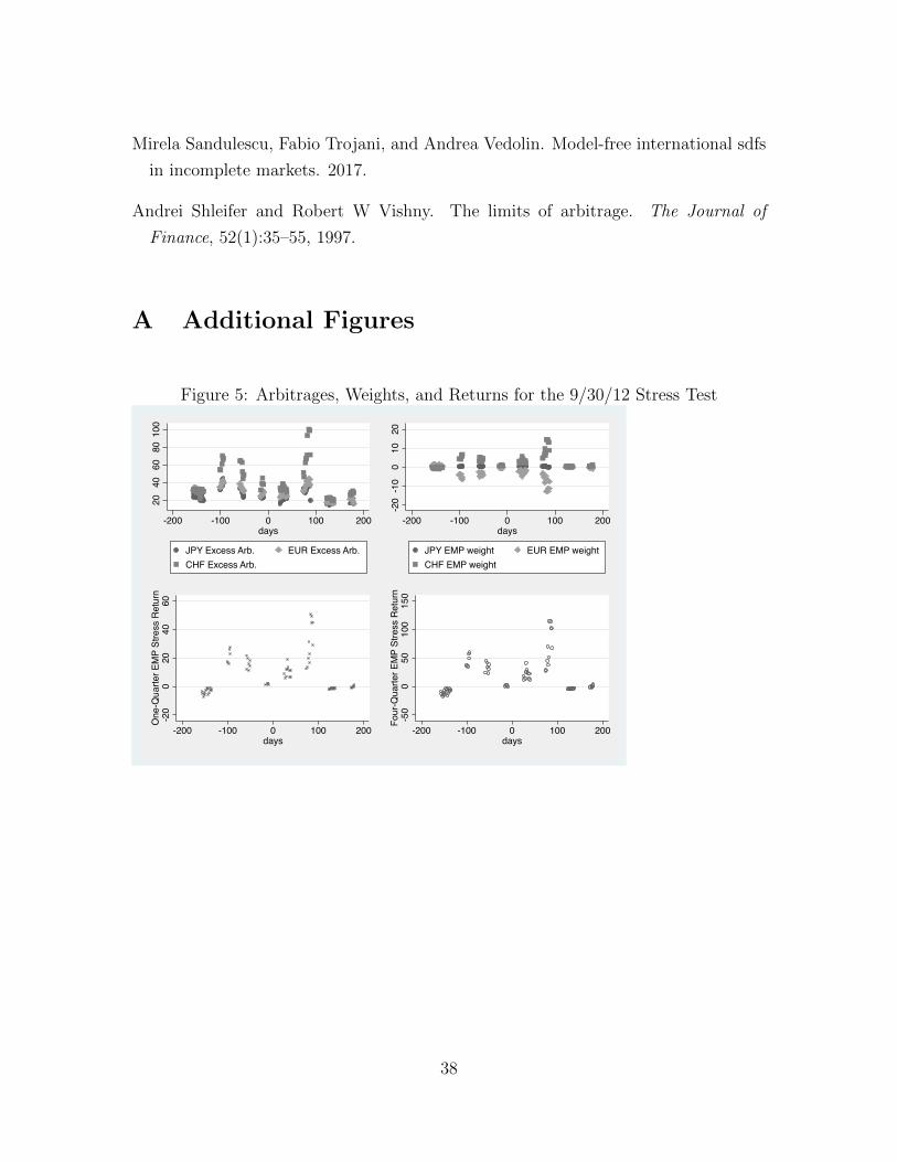
Mirela Sandulescu, Fabio Trojani, and Andrea Vedolin. Model-free international sdfs

in incomplete markets. 2017.

Andrei Shleifer and Robert W Vishny. The limits of arbitrage. The Journal of

Finance, 52(1):35–55, 1997.

A Additional Figures

Figure 5: Arbitrages, Weights, and Returns for the 9/30/12 Stress Test

2040

6080

100

-200 -100 0 100 200days

JPY Excess Arb. EUR Excess Arb.CHF Excess Arb.

-20

-10

010

20

-200 -100 0 100 200days

JPY EMP weight EUR EMP weightCHF EMP weight

-20

020

4060

One

-Qua

rter E

MP

Stre

ss R

etur

n

-200 -100 0 100 200days

-50

050

100

150

Four

-Qua

rter E

MP

Stre

ss R

etur

n

-200 -100 0 100 200days

38

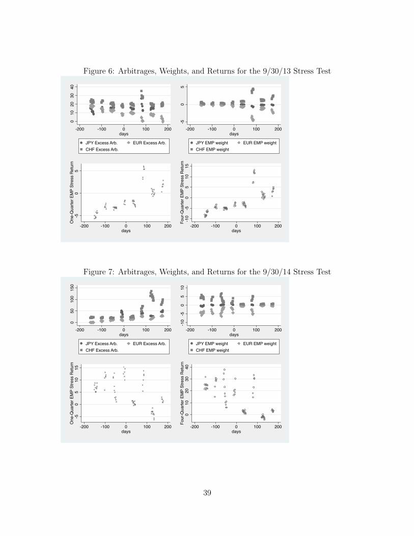
Figure 6: Arbitrages, Weights, and Returns for the 9/30/13 Stress Test0

1020

3040

-200 -100 0 100 200days

JPY Excess Arb. EUR Excess Arb.CHF Excess Arb.

-50

5

-200 -100 0 100 200days

JPY EMP weight EUR EMP weightCHF EMP weight

-50

5O

ne-Q

uarte

r EM

P St

ress

Ret

urn

-200 -100 0 100 200days

-10

-50

510

15Fo

ur-Q

uarte

r EM

P St

ress

Ret

urn

-200 -100 0 100 200days

Figure 7: Arbitrages, Weights, and Returns for the 9/30/14 Stress Test

050

100

150

-200 -100 0 100 200days

JPY Excess Arb. EUR Excess Arb.CHF Excess Arb.

-10

-50

510

-200 -100 0 100 200days

JPY EMP weight EUR EMP weightCHF EMP weight

-50

510

15O

ne-Q

uarte

r EM

P St

ress

Ret

urn

-200 -100 0 100 200days

010

2030

40Fo

ur-Q

uarte

r EM

P St

ress

Ret

urn

-200 -100 0 100 200days

39

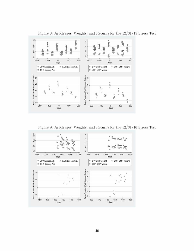
Figure 8: Arbitrages, Weights, and Returns for the 12/31/15 Stress Test0

5010

015

0

-200 -100 0 100 200days

JPY Excess Arb. EUR Excess Arb.CHF Excess Arb.

-10

12

-200 -100 0 100 200days

JPY EMP weight EUR EMP weightCHF EMP weight

-50

510

15O

ne-Q

uarte

r EM

P St

ress

Ret

urn

-200 -100 0 100 200days

010

2030

Four

-Qua

rter E

MP

Stre

ss R

etur

n

-200 -100 0 100 200days

Figure 9: Arbitrages, Weights, and Returns for the 12/31/16 Stress Test

6080

100

120

-180 -170 -160 -150 -140 -130days

JPY Excess Arb. EUR Excess Arb.CHF Excess Arb.

-10

12

3

-180 -170 -160 -150 -140 -130days

JPY EMP weight EUR EMP weightCHF EMP weight

-6-4

-20

One

-Qua

rter E

MP

Stre

ss R

etur

n

-180 -170 -160 -150 -140 -130days

-6-4

-20

24

Four

-Qua

rter E

MP

Stre

ss R

etur

n

-180 -170 -160 -150 -140 -130days

40

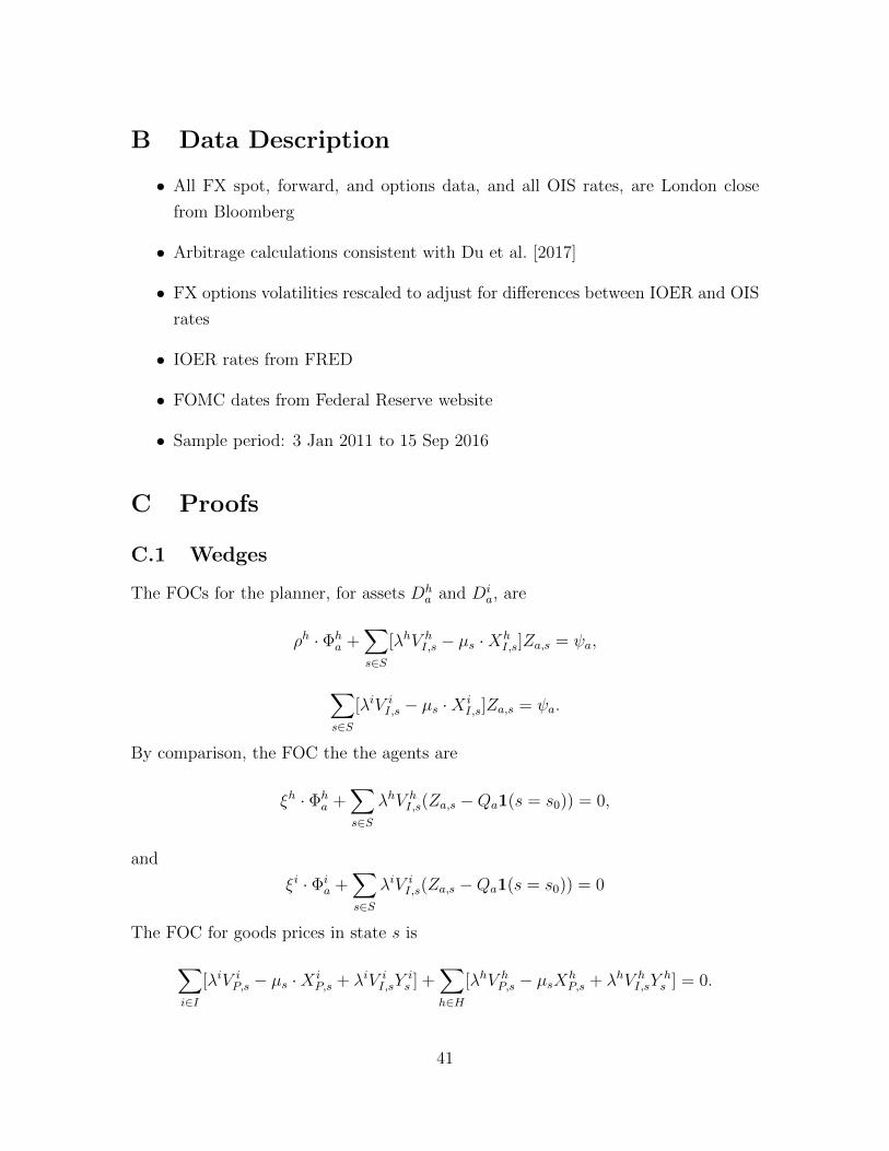
B Data Description

• All FX spot, forward, and options data, and all OIS rates, are London close

from Bloomberg

• Arbitrage calculations consistent with Du et al. [2017]

• FX options volatilities rescaled to adjust for differences between IOER and OIS

rates

• IOER rates from FRED

• FOMC dates from Federal Reserve website

• Sample period: 3 Jan 2011 to 15 Sep 2016

C Proofs

C.1 Wedges

The FOCs for the planner, for assets Dha and Di

a, are

ρh · Φha +

∑s∈S

[λhV hI,s − µs ·Xh

I,s]Za,s = ψa,

∑s∈S

[λiV iI,s − µs ·X i

I,s]Za,s = ψa.

By comparison, the FOC the the agents are

ξh · Φha +

∑s∈S

λhV hI,s(Za,s −Qa1(s = s0)) = 0,

and

ξi · Φia +

∑s∈S

λiV iI,s(Za,s −Qa1(s = s0)) = 0

The FOC for goods prices in state s is∑i∈I

[λiV iP,s − µs ·X i

P,s + λiV iI,sY

is ] +

∑h∈H

[λhV hP,s − µsXh

P,s + λhV hI,sY

hs ] = 0.

41

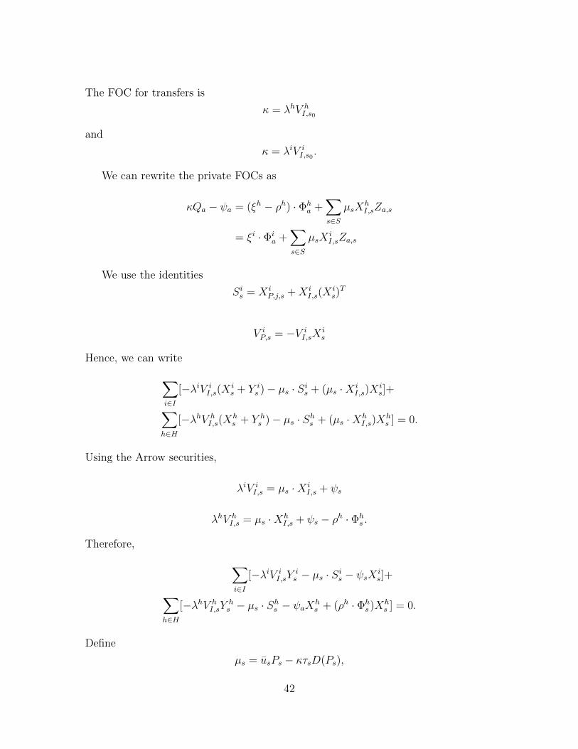
The FOC for transfers is

κ = λhV hI,s0

and

κ = λiV iI,s0.

We can rewrite the private FOCs as

κQa − ψa = (ξh − ρh) · Φha +

∑s∈S

µsXhI,sZa,s

= ξi · Φia +

∑s∈S

µsXiI,sZa,s

We use the identities

Sis = X iP,j,s +X i

I,s(Xis)T

V iP,s = −V i

I,sXis

Hence, we can write∑i∈I

[−λiV iI,s(X

is + Y i

s )− µs · Sis + (µs ·X iI,s)X

is]+∑

h∈H

[−λhV hI,s(X

hs + Y h

s )− µs · Shs + (µs ·XhI,s)X

hs ] = 0.

Using the Arrow securities,

λiV iI,s = µs ·X i

I,s + ψs

λhV hI,s = µs ·Xh

I,s + ψs − ρh · Φhs .

Therefore, ∑i∈I

[−λiV iI,sY

is − µs · Sis − ψsX i

s]+∑h∈H

[−λhV hI,sY

hs − µs · Shs − ψaXh

s + (ρh · Φhs )X

hs ] = 0.

Define

µs = usPs − κτsD(Ps),

42

so that

τs · Ps = 0.

We can rewrite the equations as∑i∈I

[−λiV iI,sY

is + κτsD(ps) · Sis − ψsX i

s]+∑h∈H

[−λhV hI,sY

hs + κτsD(ps) · Shs − ψsXh

s + (ρh · Φhs )X

hs ] = 0.

and

λiV iI,s = µs − κτsD(Ps) ·X i

I,s + ψs

λhV hI,s = µs − κτsD(Ps) ·Xh

I,s + ψs − ρh · Φha.

Using the Arrow securities and the private FOCs,

κQs − ψs = (ξh − ρh) · Φhs + us − κτsD(Ps)X

hI,s

= ξi · Φis + us − κτsD(Ps)X

iI,s

and therefore

κQs = λhV hI,s + ξhΦh

s = λiV iI,s + ξiΦi

s

Define

χa = (−Qa +∑s∈S

Za,sQs)

= κ−1ξi · (−Φia +

∑s∈S

Za,sΦis)

If an asset is tradeable by household h,

κQa − ψa = −∑s∈S

κτsD(Ps)XhI,sZa,s = ξi · Φi

a −∑s∈S

κτsD(Ps)XiI,sZa,s

43

Therefore, with no regulation of the Arrow market,

χa =∑s∈S

τsD(Ps)(XhI,s −X i

I,s)Za,s

=∑s∈S

(λi

κV iI,s −

λh

κV hI,s)Za,s

ρh · Φha +

∑s∈S

[λhV hI,s − µs ·Xh

I,s]Za,s = ψa,

∑s∈S

[λiV iI,s − µs ·X i

I,s]Za,s = ψa.

C.2 Proof of lemma 1

The divergence problem is

πh = minπ∈P(S)

Dχ2(π||πi)

subject to, for each a ∈ Aarb,

(Rh)−1∑s∈S1

πsZa,s + χa = (Ri)−1∑s∈S1

πisZa,s.

Because prices are positive, we can rescale the constraint. Defining Qia as the price

of the replicating portfolio of securities,

Qia = (Ri)−1

∑s∈S1

πisZa,s,

and Ra,s as the excess return (for all assets other than the risk-free asset),

Ra,s =

Ri a = RF

Za,s

Qia−Ri a 6= RF

,

and

χR =1

Ri− 1

Rh,

44

we can rewrite the constraint as

∑s∈S1

πsRa,s =

−Rh( χa

Qia−RiχR) a 6= RF

Ri a = RF.

Note that, for the risk-free asset, this constraint enforces that∑s∈S1

πs = 1

under the assumption that Ri > 0.

Defining the χ2 divergence

Dχ2(π||π′) =1

2

∑s∈S1

π′

s(πsπ′s− 1)2,

the Lagrangian is

minπ∈P(S1)

maxθ∈R|Aarb|,ν∈R|S|+

1

2

∑s∈S1

πis(πsπis− 1)2 −

∑s∈S1

νsπs

−∑

a∈Aarb\{aRF }

θa[∑s∈S1

(πsRa,s) +Rh(χaQia

−RiχR)]−

θRF (∑s∈S1

πsRi −Ri)

We can write the first-order condition for πs

πhsπis− 1− νs −

∑a∈Aarb

θaRa,s = 0.

where θa denotes the multiplier on the constraint. By complementary slackness, we

must have either νs = 0 or πhs = 0, and hence will have

νs = max(−1−∑a∈Aarb

θaRa,s, 0)

and

πhs = πis max(∑a∈Aarb

θaRa,s + 1, 0).

45

Under the assumption that πh has full support, νs = 0 for all s. Plugging this into

the Lagrangian, the problem solves

maxθ∈R|Aarb|

1

2

∑s∈S1

πis(∑a∈Aarb

θaRa,s)2−

∑a∈Aarb\{aRF }

θa[∑s∈S1

πisRa,s(∑

a′∈Aarb

θa′Ra′,s + 1) +Rh(χaQia

−RiχR)]−

θRF (∑s∈S1

πisRi(

∑a′∈Aarb

θa′Ra′,s + 1)−Ri),

This expression simplifies (using∑

s∈S1πisRa,s = 0 for all a ∈ Aarb \ {aRF}) to

maxθ∈R|Aarb|

−1

2

∑s∈S1

πis(∑

a∈Aarb\{aRF }

θaRa,s)2−

∑a∈Aarb\{aRF }

θa(Rh(χaQia

−RiχR))−

1

2(θRFR

i)2.

This expression is concave in θ, and the first-order condition for θa (the optimum) is∑a′∈Aarb

θa′Σia′,a =−Rh(

χaQia

−RiχR),

where Σia′,a =

∑s∈S1

πisRa,sRa′,s for a, a′ ∈ Aarb \{aRF}. Note that, trivially, θRF = 0.

Solving, for a ∈ Aarb \ {aRF},

θa′ = −RhRi∑

a∈Aarb\{aRF }

χa∑s′∈S1

πis′Za,s′− χR)(Σi)−1a,a′ .

46

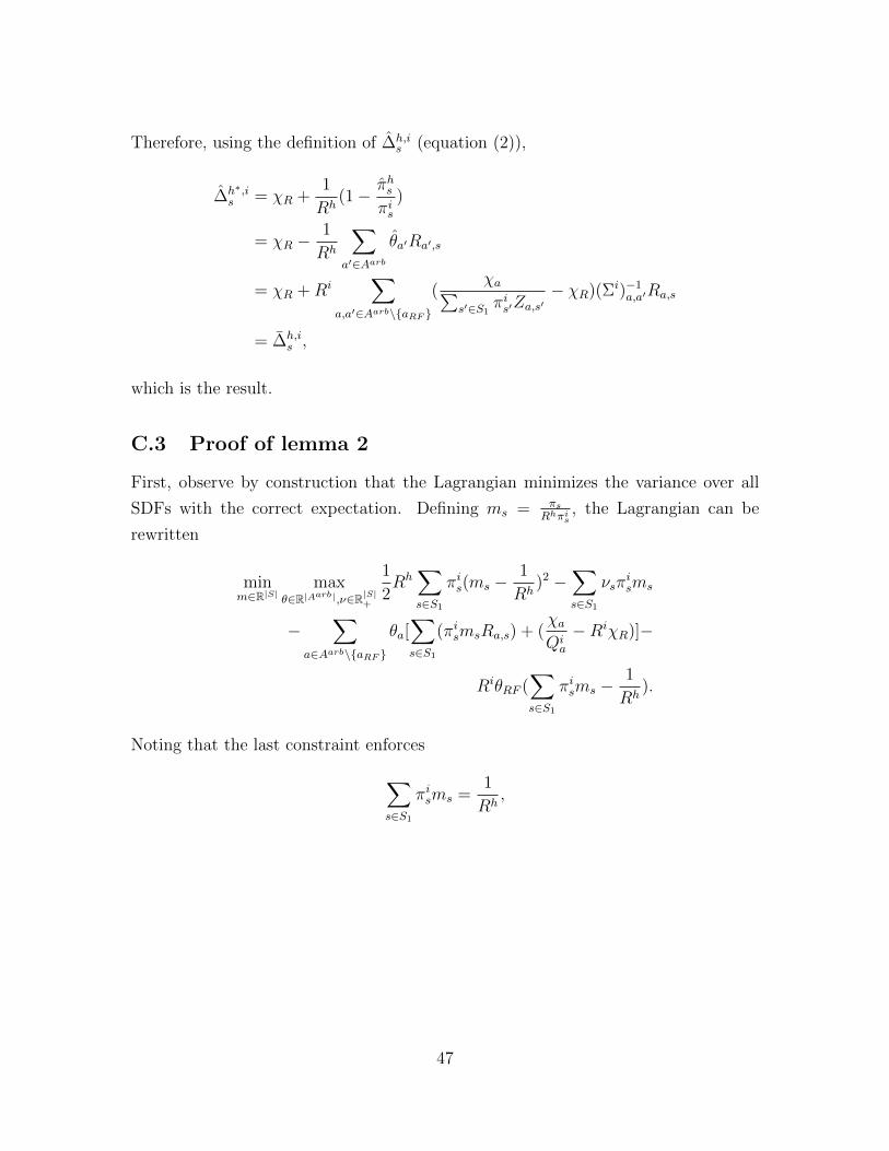
Therefore, using the definition of ∆h,is (equation (2)),

∆h∗,is = χR +

1

Rh(1− πhs

πis)

= χR −1

Rh

∑a′∈Aarb

θa′Ra′,s

= χR +Ri∑

a,a′∈Aarb\{aRF }

(χa∑

s′∈S1πis′Za,s′

− χR)(Σi)−1a,a′Ra,s

= ∆h,is ,

which is the result.

C.3 Proof of lemma 2

First, observe by construction that the Lagrangian minimizes the variance over all

SDFs with the correct expectation. Defining ms = πsRhπi

s, the Lagrangian can be

rewritten

minm∈R|S|

maxθ∈R|Aarb|,ν∈R|S|+

1

2Rh

∑s∈S1

πis(ms −1

Rh)2 −

∑s∈S1

νsπisms

−∑

a∈Aarb\{aRF }

θa[∑s∈S1

(πismsRa,s) + (χaQia

−RiχR)]−

RiθRF (∑s∈S1

πisms −1

Rh).

Noting that the last constraint enforces

∑s∈S1

πisms =1

Rh,

47

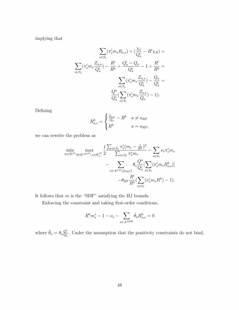
implying that ∑s∈S1

(πismsRa,s) + (χaQia

−RiχR) =

∑s∈S1

(πismsZa,sQia

)− Ri

Rh+Qia −Qa

Qia

− 1 +Ri

Rh=

∑s∈S1

(πismsZa,sQia

)− Qa

Qia

=

Qa

Qia

(∑s∈S1

(πismsZa,sQa

)− 1).

Defining

Rha,s =

Za,s

Qa−Rh a 6= aRF

Rh a = aRF ,

we can rewrite the problem as

minm∈R|S|

maxθ∈R|Aarb|,ν∈R|S|+

1

2

∑s∈S1

πis(ms − 1Rh )2∑

s∈S1πisms

−∑s∈S1

νsπisms

−∑

a∈Aarb\{aRF }

θaQa

Qia

[∑s∈S1

(πismsRha,s)]

−θRFRi

Rh(∑s∈S1

(πismsRh)− 1).

It follows that m is the “SDF” satisfying the HJ bounds.

Enforcing the constraint and taking first-order conditions,

Rhm∗s − 1− νs −∑

a∈AARB

θaRha,s = 0

where θa = θaQa

Qia. Under the assumption that the positivity constraints do not bind,

48

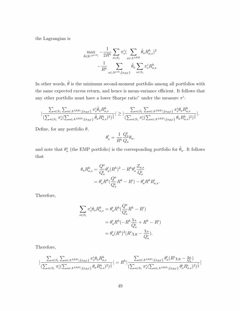
the Lagrangian is

maxθ∈R|Aarb|

− 1

2Rh

∑s∈S1

πis(∑

a∈AARB

θaRha,s)

2

− 1

Rh

∑a∈Aarb\{aRF }

θa∑s∈S1

πisRha,s

In other words, θ is the minimum second-moment portfolio among all portfolios with

the same expected excess return, and hence is mean-variance efficient. It follows that

any other portfolio must have a lower Sharpe ratio” under the measure πi:

|∑

s∈S1

∑a∈AARB\{aRF } π

isθaR

ha,s

(∑

s∈S1πis(

∑a∈AARB\{aRF } θaR

ha,s)

2)12

| ≥ |∑

s∈S1

∑a∈AARB\{aRF } π

isθaR

ha,s

(∑

s∈S1πis(

∑a∈AARB\{aRF } θaR

ha,s)

2)12

|.

Define, for any portfolio θ,

θ′a =1

Rh

Qia

Qa

θa,

and note that θ∗a (the EMP portfolio) is the corresponding portfolio for θa. It follows

that

θaRha,s =

Qa

Qia

θ′a(Rh)2 −Rhθ′a

Za,sQia

= θ′aRh(Qa

Qia

Rh −Ri)− θ′aRhRia,s.

Therefore,

∑s∈S1

πisθaRha,s = θ′aR

h(Qa

Qia

Rh −Ri)

= θ′aRh(−Rh χa

Qia

+Rh −Ri)

= θ′a(Rh)2(RiχR −

χaQia

).

Therefore,

|∑

s∈S1

∑a∈AARB\{aRF } π

isθaR

ha,s

(∑

s∈S1πis(

∑a∈AARB\{aRF } θaR

ha,s)

2)12

| = Rh|∑

a∈AARB\{aRF } θ′a(R

iχR − χa

Qia)

(∑

s∈S1πis(

∑a∈AARB\{aRF } θ

′aR

ia,s)

2)12

|

49

It follows that if there was a portfolio with a higher arbitrage Sharpe ratio than θ∗,

there would be a portfolio with a higher Sharpe ratio under πi than θ, a contradiction.

50