Embed Size (px)
Citation preview

Extensions of the Ferry shear wave model for
active linear and nonlinear microrheology
Sorin M. Mitran, M. Gregory Forest,
Lingxing Yao, Brandon Lindley1,
David B. Hill2
The Virtual Lung Project,
University of North Carolina,
Chapel Hill, 27599-3250
June 15, 2007
1Applied Mathematics Program, Department of Mathematics, University of NorthCarolina, Chapel Hill, 27599-3250
2Cystic Fibrosis Center, University of North Carolina, Chapel Hill, 27599-7248

Abstract
The classical oscillatory shear wave model of Ferry et al. [J. Polym. Sci..
2:593-611, (1947)] is extended for active linear and nonlinear microrheology.
In the Ferry protocol, oscillation and attenuation lengths of the shear wave
measured from strobe photographs determine storage and loss moduli at each
frequency of plate oscillation. Small, microliter, volumes typical in biology re-
quire modifications of experimental method and theory. Microbead tracking
replaces strobe photographs. Reflection from the top boundary yields counter-
propagating modes which are modeled here for linear and nonlinear viscoelastic
constitutive laws. Furthermore, bulk imposed strain is easily controlled, and we
explore the onset of normal stress generation and shear thinning using nonlinear
viscoelastic models. For this paper, we present the theory, exact linear and non-
linear solutions where possible, and simulation tools more generally. We then
illustrate errors in inverse characterization by application of the Ferry formu-
las, due to both suppression of wave reflection and nonlinearity, even if there
were no experimental error. This shear wave method presents an active and
nonlinear analog of two-point microrheology Crocker et al. [Phys. Rev. Lett.
85: 888 - 891 (2000)]. Nonlocal (spatially extended) deformations and stresses
are propagated through a small volume sample, on wavelengths long relative to
bead size. The setup is ideal for exploration of nonlinear threshold behavior.

Keywords: Viscoelastic shear wave; Upper convected Maxwell model; Small
sample effects; Biological fluids; Inverse characterization
1 Introduction
The unidirectional propagation of shear waves from an imposed oscillatory plate
is a classical technique for linear viscoelastic characterization of gels and poly-
mer solutions [1, 2, 3]. The experimental technique and associated modeling and
analysis are extensively discussed in the literature [4, 6, 7]. Linear viscoelastic
constitutive equations, coupled with momentum balance and boundary condi-
tions, yield an exact solution for a semi-infinite domain. In the original applica-
tions, strain-induced birefringence of synthetic polymers allows snapshots of the
propagating shear wave, from which oscillation and attenuation lengthscales are
related explicitly to frequency-dependent shear and loss moduli. These formulas
are recalled in Section 2.
Effects due to a finite depth in the direction of shear wave propagation
are negligible as long as the attenuation scale is much shorter than the gap
height, suppressing back propagation from the opposing surface; see [6], Chapter
5. The advantage of the Ferry design over various other devices carried over
from acoustics, which involve interpreting surface signals, lies in the ability to
strobe the entire shear wave as it progresses through the viscoelastic medium.
The method is therefore effective if the material is birefringent under strain,
and available in sufficient volumes. Linear response is ostensibly controlled
in the bulk by imposing sufficiently small amplitude displacements, yet the
possibility of large local strains near the source plate is evident even in the
classical snapshots. In our microrheology experiments with microliter samples,
strain-induced birefringent waves are replaced by microscopy and bead-tracking
techniques [9]. This method is appealing for various reasons:
1

• Similar to 2-point passive microrheology [13], bead time series are domi-
nated by non-local deformations and stresses rather than local bead-fluid
interactions. The signals are deterministic rather than stochastic.
• One-dimensional heterogeneity is easily modeled for general linear vis-
coelastic fluids, extending the classical viscous fluid analysis of Rayleigh
[6].
• It is straightforward to model one-dimensional heterogeneity with nonlin-
ear constitutive laws (cf. [7, 12], [14]), enabling an experimental-modeling
protocol for nonlinear inverse characterization at the low stress levels typ-
ical in human physiology. The analysis and/or numerical simulation of
the resulting system of quasilinear partial differential equations must be
developed for application to experimental data; these results are provided
in this paper.
• Selected models are capable of capturing and assessing two signature non-
linear phenomena, normal stress generation in shear and shear thinning,
which we implement to explore onset of nonlinear behavior versus plate-
induced strain.
An additional compelling feature of the Ferry shear wave experiment arises
from our interest in viscoelastic characterization of pulmonary liquids as part
of the Virtual Lung Project at UNC Chapel Hill. Namely, the oscillating plane
Couette cell mimics in vivo conditions of oscillatory transport of pulmonary
mucus by coordinated cilia and tidal breathing cycles. Thus, this method has
the potential to characterize linear and nonlinear viscoelastic properties under
conditions that approximate biological conditions. The shear wave experiment
controls oscillatory strain and frequency deformations at one fluid layer inter-
face; one can ramp up the bulk strain by controlling the amplitude of the lower
2

plate displacement relative to the height of the sample, while also monitor-
ing, with the modeling tools presented here, the local strain per wavelength
of the shear-induced deformation. Rather than rely upon refraction due to
strain-induced birefringence, Hill and Superfine [9] mix micron-scale, neutrally
buoyant beads and use particle-tracking to measure shear wave propagation fea-
tures. The model and experiment can also couple asymmetry in the imposed
plate cycle, which mimics asymmetry of the beat cycle of coordinated cilia. This
feature is easily incorporated into the framework presented here by modifying
the boundary conditions on the nonlinear solver algorithm, but that extension
is beyond the scope of the present paper. The numerical solver has also been
benchmarked in the small strain limit with exact formulas presented below, so
that this software along with inverse procedures can be used in general appli-
cations. An article focusing on the experimental protocols and applications to
benchmark viscoelastic fluids and biological liquids is in preparation [8].
This method for viscoelastic constitutive characterization holds special promise
for applications in other biological systems as well, where samples are often only
available in small volumes. The modeling and assessment of counterpropagat-
ing waves and nonlinearity versus imposed strain, especially in regard to inverse
characterization, are the primary contributions of this paper. We show in the
present paper that accuracy of the classical Ferry formulas varies significantly
depending on viscoelastic moduli versus frequency, imposed displacement am-
plitude, and sample height. For example, a conservative estimate of wave speeds
for 30μm thick samples of a viscoelastic material, based on reported ranges of
bulk moduli in pulmonary liquids, indicates multiple wave reflections within
each period of plate oscillation in 10 − 20Hz frequency range. From simulated
finite depth data for prescribed viscoelastic moduli, thereby removing any ex-
perimental error, we show that fitting to formulas based on unidirectional waves
3
can lead to enormous errors in inverse recovery of the moduli.
The key issue motivating this paper is whether the assumptions of the Ferry
model, linearity and a semi-infinite domain, are approximately satisfied under
experimental conditions with limited volumes. More precisely, we assess accu-
racy of the linear, semi-infinite assumption across a multiple parameter space:
storage and loss moduli versus frequency, gap height, and plate displacement
amplitude. The infinite depth assumption is surely not valid, so the first target
is to assess the order of errors in storage and loss moduli across some frequency
range, due to this effect alone. Next, we aim to characterize the threshold
strain (imposed by the lower plate displacement relative to sample height) at
which nonlinear effects become significant, and to assess measurable flow and
stress features triggered by nonlinearity. It is hypothesized that normal stresses
in shear, a standard signature of nonlinearity, play an important role in pul-
monary liquid transport by coordinated cilia and coughing events. A possible
scenario is that normal and shear stresses propagate from the mucus and peri-
ciliary liquid layer to the epithelium, causing cellular compressive and shear
strain, serving to regulate biochemical feedback. The role of shear thinning in
pulmonary transport is not known, so a method is desirable that can simply
ascertain whether a given sample shear thins under controlled strain conditions.
The remainder of this paper is organized as follows. Section 2 gives a sum-
mary of models, from linear–viscous to nonlinear–viscoelastic. Section 3 con-
tains analytical results, including exact solutions and formulas for linear and
nonlinear, semi-infinite and finite depth, models, as well as analysis of well-
posed boundary conditions for the nonlinear models. Section 4 contains numer-
ical studies of the two nonlinear models, their comparison to linear models and
one other, and a discussion of physical predictions.
4

2 Shear wave models
2.1 Physical parameters and non-dimensionalization
We consider a layer of incompressible fluid of height H , set into motion by
an oscillating lower flat plate, and whose upper surface remains flat and par-
allel to the bottom plate. The˜ superscript will be used to denote quantities
expressed in physical units. The bottom plate is set into harmonic motion
V (t) = V0 sin(ωt), as illustrated in Figure 1.
Figure 1: Schematic of oscillatory Couette flow and notation used to describethe deviatoric stress on an infinitesimal fluid element. The x-axis is parallel tothe plate motion, the y-axis is the cross-channel direction.
A reference viscosity η0 value is chosen for the fluid of interest, namely the
zero strain-rate viscosity of the fluid. The reference length A = V0/ω is the
5

maximum displacement of the driven plate; the reference time ω−1 is set by the
plate frequency; and the reference stress η0ω is the viscous plate shear stress.
With this choice, the non-dimensional velocity of the bottom plate is given by
vx(0, t) = V (t) = sin(t), where vx(y, t) denotes the velocity component of the
fluid in the direction of plate motion at height y. It is a property of the model
equations that with this scaling, we can focus on the 2-parameter space of
values of storage and loss moduli, and make general statements about errors in
recovering the moduli that depend only on the pair of values, independent of the
imposed frequency. We return later to the practical implications of this scaling
property. Typically, a distinguished material relaxation time λ is identified,
the ratio of a viscosity to an elastic modulus. The following dimensionless
parameters arise in the model equations:
• Reynolds number Re = ρωA2/η0
• Deborah number λ = λω
• Bulk shear strain γ = A/H.
By symmetry, the one-dimensional propagation of velocity and stress leads
to the following reductions in flow and stress variables, all functions only of t
and the height y between the two flat surfaces. The fluid pressure p and velocity
components are
p = p(y, t), vx = vx(y, t), vy = 0, vz = 0. (1)
From vx(y, t), we may construct transient particle displacements X(y, t) at each
height (y) in the layer,
X(y, t) =∫ t
0
vx(y, t′)dt′ +X(y, 0), (2)
6

for given initial conditions X(y, 0).
The fluid motion is determined from the non-dimensional momentum equa-
tion,∂v
∂t+ (v ·�)v =
1Re
�·(−pI + τ ), (3)
together with a constitutive law for the extra stress, τ , which likewise is assumed
to depend only on t and y,
τ = τ (y, t), with τxz = τyz = 0. (4)
To close the system for (p, vx, τ )(y, t), we require the constitutive law relating
τ and �v. A hierarchy of laws has been discussed in standard texts [6], [7, 12],
the elements of which we now recall.
2.2 Newtonian Viscous Fluid
For viscous fluids, the Navier-Stokes constitutive law is
τ = 2D, (5)
where D ≡ 12 (�v + �vT ), is the rate-of-strain tensor (the viscosity coefficient
does not appear due to the scaling, 2.1). From (1), it follows that
⎧⎪⎪⎨⎪⎪⎩τxy =
∂vx
∂y,
τxx = τyy = τxz = τyz = τzz ≡ 0.(6)
The momentum equation (3) reduces to
⎧⎪⎪⎨⎪⎪⎩∂vx
∂t=
1Re
∂2vx
∂y2,
∂p
∂y= 0 .
(7)
7

2.3 Linear Viscoelastic Fluids
The constitutive law of linear viscoelasticity (the Lodge model) is
τ = 2∫ t
−∞G(t− t′)D(y, t′)dt′, (8)
where G(t) is the non-dimensional shear relaxation modulus function. In phys-
ical units we have G = η0ωG. Combining (1) and (8), only shear stresses are
generated: ⎧⎪⎪⎨⎪⎪⎩τxy =
∫ t
−∞G(t− t′)
∂vx
∂y(y, t′)dt′,
τxx = τyy = τxz = τyz = τzz = 0.
(9)
The momentum equation (3) closes the system:
∂vx
∂t=
1Re
∂τxy
∂y, (10a)
∂p
∂y= 0. (10b)
From (9) and (10a), a closed equation for vx follows:
∂vx
∂t=
1Re
∫ t
−∞G(t− t′)
∂2vx
∂y2(y, t′)dt′, (11)
and then the shear stress is calculated from (9).
We note for future reference that if the shear modulus G(t) is a single-mode
Maxwell model, G(t) = (ηp/λ) e−t/λ (non-dimensional form), then the equation
(11) simplifies to a damped wave equation for vx (cf. [6, 7]),
∂2vx
∂t2− ηp
λ Re
∂2vx
∂y2+
1λ
∂vx
∂t= 0. (12)
Furthermore, it is straightforward to show that the shear stress τxy satisfies the
8

identical damped wave equation (12).
2.4 Upper Convected Maxwell and Giesekus Models of
Nonlinear Viscoelasticity
The standard procedure for lifting linear viscoelasticity to nonlinear regimes is
treated in classical texts [7, 12]. Either one pursues the K-BKZ class of integral
constitutive laws, generalizing (8), or one pursues differential laws, the choice
made here. This approach begins with a decomposition of the extra stress into
a finite sum,
τ =k∑
i=1
τ i, (13)
where each τ i obeys a Maxwell-type evolution equation, with nonlinearity through
the upper convected derivative as well as other nonlinear terms that have been
developed to capture specific nonlinear properties. We will explore a Giesekus
model below which extends the Upper Convected Maxwell model to include
shear thinning capability. For the remainder of this paper, we restrict to a
single Maxwell-type mode; the extension to any finite number of modes is nu-
merically straightforward, where the numerical cost scales proportional to the
number of modes.
The Maxwell-type evolution equation for the extra stress is
λ∇τ = 2ηpD− τ − a τ τ , (14)
where the upper convected derivative∇τ is defined by
∇τ =
∂τ
∂t+ (v · ∇) τ − (∇v)T τ − τ (∇v). (15)
In this type of model the additional polymeric stress τ is transported by the
9

velocity field v, decays exponentially at rate λ, is produced by the solvent fluid
rate of strain D (with scaling 2ηp/λ, ηp = ηp/η0) and is nonlinearly modified
through the Giesekus term (a/λ) τ τ . The Giesekus “mobility parameter” a
distinguishes various viscoelastic models: a = 0 reduces to the upper convected
Maxwell (UCM) model, while a = 0.5 is the Leonov model. In general, it is
assumed that 0 ≤ a ≤ 1, and the mobility parameter is to be fitted from data
along with λ.
For the oscillatory-plate problem the polymeric stress transport equations
(14) become
⎧⎪⎪⎪⎪⎪⎪⎪⎪⎨⎪⎪⎪⎪⎪⎪⎪⎪⎩
∂τxx
∂t− 2τxy
∂vx
∂y= − 1
λτxx − a
λ(τ2
xx + τ2xy)
∂τxy
∂t− τyy
∂vx
∂y=ηp
λ
∂vx
∂y− 1λτxy − a
λτxy (τxx + τyy)
∂τyy
∂t= − 1
λτyy − a
λ(τ2
xy + τ2yy)
τyz = τxz = τzz = 0 .
(16)
The momentum equation reduces to
∂vx
∂t=
1Re
∂τxy
∂y, (17a)
∂p
∂y=∂τyy
∂y. (17b)
The upper convected derivative,∇τ , and the shear thinning term τ τ , render
the stress transport equations nonlinear. As in the Newtonian fluid case, there
is no convective nonlinearity in the momentum equation itself. An important in-
dicator of nonlinearity is the shear-induced generation of a non-zero first normal
stress difference, N1 = τxx − τyy, an easily measured feature. The presence of a
normal stress gradient along the y-direction then generates a pressure gradient,
absent in the linear model. Indeed, neglecting all nonlinear terms from (16)
10

the two normal stress components τxx, τyy, obey identical ordinary differential
equations∂τxx
∂t+
1λτxx = 0,
∂τyy
∂t+
1λτyy = 0 . (18)
Thus, there is no possibility of generation of normal stresses in shear flow under
linear assumptions. Additionally, any initial normal stresses distributed across
the layer relax exponentially fast, and do not propagate nor couple to the shear
stress and shear wave. Finally, the Giesekus model captures shear thinning. All
nonlinear features are addressed in the context of the numerical results.
The coupled system (16) and (17a) can be written as an evolution equation,
∂q
∂t+A(q)
∂q
∂y= ψ(q), (19)
with
q =[vx τxx τxy τyy
]T,
A(q) =−
⎡⎢⎢⎢⎢⎢⎢⎢⎣
0 0 1/Re 0
2τxy 0 0 0
ηp/λ+τyy 0 0 0
0 0 0 0
⎤⎥⎥⎥⎥⎥⎥⎥⎦, ψ = − 1
λ
⎡⎢⎢⎢⎢⎢⎢⎢⎣
0
τxx + a (τ2xx + τ2
xy)
τxy+a τxy (τxx +τyy)
τyy + a (τ2xy + τ2
yy)
⎤⎥⎥⎥⎥⎥⎥⎥⎦,
together with the pressure equation (17b) and τxz = τyz = 0.
2.5 Boundary conditions
Boundary conditions are required at the bottom plate y = 0, which is experi-
mentally controlled, and at the top boundary y = H , which may or may not
be explicitly controlled. The system of partial differential equations (19) is hy-
perbolic if the normal stress τyy obeys an inequality (see Sect. 3.3.1). If the
11

inequality is violated, the model is no longer well-posed for the study of this
experiment, a common occurrence for Maxwell-type models (cf. [14]). Hence,
the characteristics of the system must be investigated to determine allowable
boundary conditions. The following physically motivated conditions are ana-
lyzed in Sec. 3.3.2.
2.5.1 Lower plate boundary condition
At y = 0, no-slip boundary conditions apply, so that
vx(y = 0, t) = V (t), (20)
with V (t) the imposed velocity of the lower plate. From (2) and for harmonic
plate motion V (t) = sin(t), the plate displacement is given by
X(0, t) =∫ t
0
V (s)ds +X(0, 0) = (1 − cos t) +X0, (21)
where X0 labels the horizontal plate coordinate at t = 0.
2.5.2 Top boundary condition
We distinguish two types of top (flat) interface conditions:
1. The top of the layer is in contact with a flat plate, which could be held sta-
tionary or allowed to move (in which case the velocity at the top boundary
is imposed)
vx(y = H, t) = VH(t). (22)
The stationary top plate condition is the most readily realized experimen-
tal condition when seeking inverse characterization.
2. The top of the layer is in contact with another fluid, in which case conti-
12
nuity of shear stress yields
τxy(y = H, t) = τxy(H, t) of the ambient fluid. (23)
The simplest case is to assume a passive ambient so that the shear stress
is identically zero.
We address the issue of normal stress boundary conditions in the character-
istic analysis below.
3 Analytical results
For viscous and linear viscoelastic fluids, with semi-infinite and finite domains,
the model equations above are exactly solvable by Fourier methods if one ignores
transients, and further solvable with transients by Laplace methods. The tradi-
tional approach (cf. Ferry [6]) is to suppress transients, leading to closed form
solutions whose experimentally measurable features (e.g. attenuation length
and shear wavelength) are explicitly related to material properties. Thus in-
verse characterization is given by simple formulas. We review these results now
with some extensions that appear to be absent in the literature. The numerical
solutions, naturally, can easily be used to model transients. We further show
that the nonlinear model for an upper convected Maxwell law is also exactly
solvable, and therefore explicit representations for normal stress generation in
shear are determined. The Giesekus model does not submit to a closed-form
solution.
3.1 Viscous fluid solution
The long-time solution for the viscous model (7) is widely available (e.g. [5])
and recalled for completeness as well as comparison with generalizations.
13

Semi-infinite domain solution. Upon positing a solution of the form
vx(y, t) = Im{vx(y)eit} (recall time is measured in units of ω−1, so the physical
frequency is ω/2π), the solution is given by
vx(y, t) = Im{e−δ0y eit}
= e−α0y sin(t− β0y)
which obeys the far-field boundary condition limy→∞ vx(y, t) = 0. We have in-
troduced δ0 = α0 + iβ0 =√i Re = (1 + i)
√Re/2. The Reynolds number,
Re = ρωA2/η0, determines both the penetration (1/α0) and oscillation length-
scales (2π/β0), through α0 = β0 =√Re/2. The velocity field produces a
particle displacement
X(y, t) = X(y, 0) + e−α0y [cos(βt) − cos(t− βy)]
The viscous shear stress is given by τxy = ∂vx/∂y,
τxy(y, t) = Im{−δ0 e−δ0yeit}
= sin(t− β0y + 5π/4)e−α0y√Re ,
showing a constant phase difference φ = 5π/4 between the shear stress and the
velocity.
Finite-depth channel with stationary top plate. The no-slip boundary
condition at the top of the channel reads vx(y = H, t) = 0. The solution is simple
vx(y, t) = Im{eit sinh [δ0 (H − y)]
sinh [δ0 H ]
}, (24)
but does not appear to have been written down in the literature.
14

3.2 Linear viscoelastic model solutions
We summarize the Fourier, frequency-locked solutions to (10a - 10b) with the
bottom plate forcing V (t) = sin(t), ignoring transients.
Semi-infinite domain solution [6]. If the loss modulus is non-zero, then
vx(y → ∞, t) = 0. (25)
A separable Fourier solution is posited, vx(y, t) = Im{vx(y)eit}. Then from (9)
and (10a) a simple ordinary differential equation for vx(y) is obtained,
d2vx
dy2− i Re
η∗vx = 0. (26)
where the non-dimensional complex viscosity η∗ =∫∞0 G(s) exp(−is)ds = η′ −
iη′′, has been introduced. For a Maxwell model with G(s) = (ηp/λ)e−s/λ we
obtain
η′ =ηp
1 + λ2, η′′ =
ηpλ
1 + λ2. (27)
The decay condition (25) selects one independent solution of (26), and the
velocity has the same form as the viscous solution:
vx(y, t) = Im{eite−δy}
= e−αy sin(t− βy) , (28)
where δ = α+ iβ =√i Re/η∗, (α, β ∈ R+),
α =
√Re/2|η∗|
√|η∗| − η′′, β =
√Re/2|η∗|
√|η∗| + η′′ . (29)
15

For the single mode Maxwell fluid
α2 =Re
2
√1 + λ2 − λ
ηp=
12c2
(√1λ2
+ 1 − 1
), (30)
β2 =Re
2
√1 + λ2 + λ
ηp=
12c2
(√1λ2
+ 1 + 1
), (31)
where the zero-stress shear wave speed c =√ηp/(λ Re) has been introduced.
Clearly, 0 < α ≤ β, with equality only in the viscous limit η′′ = 0, η∗ = 1
(λ = 0, ηp = 1) such that α = β =√Re/2. The greater the elastic component
η′′, the larger the difference between the oscillation wavelength 2π/β and the
attenuation length 1/α.
The transform of the complex modulus, G(ω) = G′ + iG′′, in our choice of
non-dimensional units, is related to the complex viscosity η(ω) by G = iη∗; in
dimensional units, G = iωη∗. The non-dimensional formulas relating storage
and loss moduli and the reciprocal lengthscales α and β are:
G′ =
(β2 − α2
)Re
(α2 + β2)2, G′′ =
2αβ Re
(α2 + β2)2. (32)
Re-expressing the above formulas in physical quantities recovers the formulas of
Ferry, Sawyer, and Ashworth [6]
G′ = ρω2
(β2 − α2
)(α2 + β2
)2 , G′′ = ρω2 2αβ(α2 + β2
)2 ,
used to infer G′(ω), G′′(ω) from experimental measurements of α = αA, β = βA.
The particle positions X(y, t) at height y are then given by
X(y, t) = X(y, 0) + e−αy [cos(βy) − cos(t− βy)] . (33)
16

The shear stress can be computed using the Lodge stress formula (8)
τxy(y, t) = Im{∫ t
−∞G(t− t′)
dvx
dy(y)eit′ dt′
}= Im
{η∗dvx
dy(y)eit
}.
For the velocity (28) we obtain,
τxy(y, t) = Im{−δη∗eite−δy}
= sin(t− βy + φ+ π)e−αy√|η∗|Re , (34)
and, of course, the normal stresses are identically zero for linear viscoelasticity,
τxx = τyy = τzz = 0. The phase shift of the tangential stress with respect
to the velocity is φ + π, with φ = arctan(β/α), 0 ≤ φ ≤ π/2. Note that
the stress required to achieve the claimed boundary condition on plate speed is
τxy(y = 0, t) = − sin(t+ φ)√|η∗|Re.
A comparison to the viscous solution is informative. The ratio of the viscous
to viscoelastic penetration lengths (α/α0) is shown in Fig. 2. When η′′ = 0
we obtain the expected increase in penetration depth as η′ increases – a more
viscous fluid leads to more momentum transfer from the oscillating plate. As
the fluid elasticity η′′ increases, the penetration depth ratio decreases. Some of
the momentum imparted to the fluid by the oscillating plate is now radiated
as an elastic shear wave, hence the penetration depth is smaller. The ratio of
viscid to viscoelastic wavelengths (β/β0) is also shown in Fig. 2. For viscoelastic
fluids with η′′ > 0 the wavelength reflects the competition between diffusive and
radiative momentum transfer. At a given η′ an initial increase in the elasticity
decreases the wavelength. In this range the motion is overdamped and the
decrease in penetration depth dominates the wavelength. At greater values of
η′′ the radiative momentum transfer (through shear waves) becomes dominant
and there is an increase in the wavelength. The maximum viscoelastic shear
stress is greater than the purely viscous stress by a factor of√|η∗| and exhibits
17

a different phase shift, φ+ π instead of 5π/4.
2 4 6 8 100.0
0.2
0.4
0.6
0.8
1.0
Η'
Α�Α0
Penetration Length Ratio
2 4 6 8 100.00.20.40.60.81.01.2
Η'
Β�Β0
Wavelength Ratio
�� � 2
�� � 2�� � 0
�� � 0
�� � 10
�� � 10
Figure 2: Comparison of viscoelastic penetration (1/α) and wave lengths (2π/β)to the viscous values (1/α0, 2π/β0)
Finite channel depth. When the fluid is bounded above at y = H by a
flat interface moving at velocity vH(t), a no-slip boundary condition yields
vx(y = H, t) = vH(t) .
The Fourier method used here ignores transients and can only be used for top
plate velocities of the form vH(t) = VHeit with VH some complex constant
giving the amplitude of the top plate motion as well as its relative phase with
respect to the bottom plate forcing. The solution in this case is given by
vx(y, t) = Im{eit sinh [δ(H − y)]
sinh (δH)+ VHe
it sinh (δy)sinh (δH)
}. (35)
The most easily controlled experimental condition is to place a stationary solid
lid on the top interface in which case VH = 0,
vx(y, t) = Im{eit sinh [δ(H − y)]
sinh (δH)
}. (36)
18

The half-plane solution (28) is recovered in the limit H → ∞
limH→∞
sinh [δ(H − y)]sinh (δH)
= e−δy, limH→∞
sinh (δy)sinh (δH)
= 0, (37)
recalling that δ = α + iβ and α > 0. (This “textbook” solution does not ap-
pear to be in the literature; it is given here for explicit comparison with the
semi-infinite solution, and since it is the basis for finite-depth inverse character-
ization.) The stress is given by
τxy(y, t) = Im{−δ η∗ cosh[δ (H − y)]
sinh(δ H)eit
}
Finite channel depth, flat fluid-fluid boundary above. The boundary
condition in this case is continuity of tangential stress within the viscoelastic
fluid τyx(H, t) and the adjacent fluid τH(t). Again, because we are neglecting
transients, the adjacent fluid must exhibit a tangential stress dependence of the
form τH(t) = THeit to be consistent with the Fourier procedure. This leads to
dv0x
dy(y = H) =
TH
η∗, (38)
and the solution
vx(y, t) = Im{eit
[cosh [δ(H − y)]
cosh (δH)+TH
η∗δsinh(δy)cosh(δH)
]}. (39)
This solution is relevant if one solves the model equations for the fluid layer
above, or designs an experiment with a controlled dynamic shear stress at the
interface. (This solution likewise appears not to have been previously pub-
lished.)
It should be noted however that ensuring that the top fluid layer has the
simple harmonic tangential stress τH(t) = THeit is difficult to realize experi-
19

mentally. If the adjacent fluid exerts negligible stress upon the viscoelastic fluid
layer TH∼= 0, then the formula
vx(y, t) = Im{eit cosh [δ(H − y)]
cosh (δH)
},
is valid. Otherwise, it is to be expected that τH(t) contains other frequencies
besides the fundamental frequency used in the bottom plate forcing eit. Should
one attempt, irrespective of this observation, to use formula (39), then the
complex viscosity deduced from the experimental measurements will be affected
by aliasing of the additional frequencies present in τH(t) onto the fundamental
mode eit.
Linear model limitations. The constitutive law (8) is valid for small
strains
max |Dxy| = max∣∣∣∣∂u∂y∣∣∣∣ = max
∣∣∣∣ ∂∂y∫ t
0
vx(y, s)ds∣∣∣∣ 1 .
For the half-plane solution (28) the strain is given by
Dxy(y, t) = e−αy {α [cos(t− βy) − cos(βy)] + β [sin(t− βy) + sin(βy)]}
assuming X(y, 0) = 0. Physically we expect the maximum strain to be obtained
at y = 0 where the displacement is
X(y = 0, t) = −α (1 − cos t) − β sin t .
The extremum ofX(0, t) is obtained when cos t = α/√α2 + β2, sin t = −β/
√α2 + β2,
hence
max |Dxy| =√α2 + β2 − α .
20

Since√α2 + β2 =
√Re/|η∗|, the small strain condition becomes
√Re
|η∗|
(1 −√
|η∗| − η′′
2 |η∗|
) 1 .
The elastic limit of fluid behavior corresponds to η′′ � η′ for which the small
strain condition becomes
Re η′′ .
It is useful to revert to physical units to highlight the significance of these limits.
Recall that Re = ρωA2/η0 and G′ = ωη′′. The small strain condition in the
elastic limit then states that
ρ(ωA)2 G′ ,
or, physically, that the dynamic pressure induced by the oscillating plate must
be much less than the elastic modulus of the fluid. In the viscous limit η′ =
1, η′′ = 0, the small-strain condition becomes√Re 1 . In physical terms this
states that
A d =√ω/2ν ,
or that the amplitude A of the oscillating bottom plate must be much less than
the viscous penetration depth d. If viscous and elastic effects are roughly equal,
η′ ∼= η′′, then the small strain condition becomes
Re << min(η′, η′′) .
The coefficients (η′, η′′) obtained from fitting experimental data to the formulas
above should be checked against these limits to ascertain whether non-linear
effects are insignificant. In the finite-depth linear and nonlinear models, one
21

can calculate the local strain from the numerical solutions, which generically
will be maximal in the first half-wavelength of the shear deformation at the
lower plate.
3.3 Nonlinear model solution in special limits
3.3.1 Hyperbolic system structure
We now turn to a consideration of nonlinear effects by solving (19). If the
system obeys the linear limit, that will become evident from the solution. Our
focus is conditions where nonlinear effects are measurable. In general numerical
methods are required for a solution. We present the analysis needed for such
numerical methods. For the upper convected Maxwell model, quite conclusive
analytical results are attainable.
The matrix A from (19) has eigenvalues μ1 = μ2 = 0, μ3 = − c, μ4 = c with
c =√ηp/(λRe) + τyy/Re , (40)
denoting the velocity of propagation of shear waves transverse to the flow direc-
tion. If the fluid is elastic to some extent, then λ > 0 and finite. Furthermore
if τyy ≥ 0 then the shear wave velocity c is a real number. It is interesting
to note that for a given relaxation time λ there exists a critical normal stress
τyy = −ηp/λ at which c = 0, and for τyy < −ηp/λ, the system is no longer
hyperbolic, but elliptic. The associated right eigenvectors are
R =[r1 r2 r3 r4
]=
⎡⎢⎢⎢⎢⎢⎢⎢⎣
0 0 −c c
0 1 2τxy 2τxy
0 0 c2Re c2Re
1 0 0 0
⎤⎥⎥⎥⎥⎥⎥⎥⎦. (41)
22

The eigenvectors form a basis for real c = 0, hence the system (19) is hy-
perbolic. The structure of this system is particularly simple with two non-
propagating components, whose physical significance will be addressed below.
The multiplicity-two zero characteristic speed allows considerable analytical
progress.
Consider a local linearization in which we use average values (denoted by an
overbar) in the eigenvector expressions
R =
⎡⎢⎢⎢⎢⎢⎢⎢⎣
0 0 −c c
0 1 2τxy 2τxy
0 0 c2Re c2Re
1 0 0 0
⎤⎥⎥⎥⎥⎥⎥⎥⎦, R
−1 =1
2c2
⎡⎢⎢⎢⎢⎢⎢⎢⎣
0 0 0 2c2
0 2c2 −4τxy/Re 0
−c 0 1/Re 0
c 0 1/Re 0
⎤⎥⎥⎥⎥⎥⎥⎥⎦.
The characteristic variables of the problem are
w =
⎡⎢⎢⎢⎢⎢⎢⎢⎣
w1
w2
w3
w4
⎤⎥⎥⎥⎥⎥⎥⎥⎦= R
−1q =
⎡⎢⎢⎢⎢⎢⎢⎢⎣
τyy
τxx − 2τxy/(c2Re)τxy
−vx/2c+ τxy/(2c2Re)
vx/2c+ τxy/(2c2Re)
⎤⎥⎥⎥⎥⎥⎥⎥⎦,
and (19) can be rewritten in terms of these variables as
∂w
∂t+ Λ
∂w
∂y= φ (42)
with Λ = diag {μ1, μ2, μ3, μ4} and φ = R−1ψ,
φ = − 1λ
⎡⎢⎢⎢⎢⎢⎢⎢⎣
τyy + a(τ2xy + τ2
yy
)τxx + a
(τ2xy + τ2
xx
)− 4τxy σ
σ
σ
⎤⎥⎥⎥⎥⎥⎥⎥⎦, σ =
τxy
2c2Re(1 + a (τxx + τyy)) .
23

The forcing term φ can be rewritten as a function of the characteristic variables
φ = φ(w) by using the transformation,
q = Rw =
⎡⎢⎢⎢⎢⎢⎢⎢⎣
c(w4 − w3)
w2 + 2τxy(w3 + w4)
c2(w3 + w4)Re
w1
⎤⎥⎥⎥⎥⎥⎥⎥⎦. (43)
3.3.2 Characteristic boundary conditions
The hyperbolic structure of the problem indicates the compatible physical bound-
ary conditions that must be used in numerical simulations. The non-propagating
quantities w1 = τyy and w2 = τxx − 2τxy
ρc2 τxy can be freely specified initially on
the bottom and top boundaries. Subsequent values must be determined by
solving the ordinary differential equations at each boundary
∂w1
∂t= − 1
λ
[τyy + a
(τ2xy + τ2
yy
)], (44)
∂w2
∂t= − 1
λ
[τxx + a
(τ2xy + τ2
xx
)− 4τxy σ].
At the bottom plate (y = 0) only the w4 = − 12cvx + 1
2ρc2 τxy quantity can be
specified as a boundary condition since it is propagating into the fluid from the
adjacent domain. The quantity w3 = 12cvx + 1
2ρc2 τxy propagates from within
the fluid domain towards the boundary and must be determined as part of the
solution procedure. Conversely, at the top boundary (y = H) w3 can be given as
a boundary condition and w4 results from the solution procedure. Typically, we
wish to give boundary conditions in terms of the physical variables. The essence
of the above discussion is that we cannot impose both vx and τxy at boundaries.
To do so would determine both w3 and w4 in violation of characteristic infor-
mation propagation directions. We list common cases of compatible boundary
24

conditions which inform experimental protocols for this class of models to be
applicable.
1. Velocity and normal stresses. At the bottom plate we specify vx and
propagation from within the channel as specified by the characteristic
equation∂w3
∂t− c
∂w3
∂y= −σ/λ, (45)
gives w3. This allows τxy = 2 Re c2(w3 + 1
2cvx
)to be computed. We
solve (44) to obtain w1, w2. Using (43) we then compute τxx, τyy thereby
obtaining all the variables within the q vector. At the top plate we proceed
analogously, by specifying vx but obtaining τxy from the w4 component
as τxy = 2 Re c2(w4 − 1
2cvx
). The w4 component is determined from
propagation within the fluid by solving
∂w4
∂t+ c
∂w4
∂y= −σ/λ . (46)
2. Tangential and normal stresses. At both boundaries we specify τxy. Solv-
ing (44) gives w1, w2 and hence τyy, τxx. At the bottom boundary vx is
obtained from the propagating w3 component by solving (45) and at the
top from the w4 component obtained by solving (46).
3. Non-reflective top boundary condition. To simulate an infinite domain
we can set the incoming characteristic at y = H � 1 to zero, w3 = 0.
Numerically, care must be taken so there are no spurious reflections of the
w4 component at the y = H boundary.
Figure 3 gives a graphical overview of the procedure used to set boundary
conditions.
25

Figure 3: Geometry of characteristics of system (19) near the boundaries, high-lighting characteristics coming from inside the computational domain (w3 aty = 0, and w4 at y = H) and non-propagating characteristic variables w1, w2.
3.3.3 Upper convected Maxwell (UCM) solution
After the general analysis presented above let us consider an exactly solvable
case. For the UCM model we have a = 0 and the system (19) becomes
⎧⎪⎪⎪⎪⎪⎪⎪⎪⎪⎨⎪⎪⎪⎪⎪⎪⎪⎪⎪⎩
∂vx
∂t− 1Re
∂τxy
∂y= 0
∂τxx
∂t− 2τxy
∂vx
∂y= − 1
λτxx
∂τxy
∂t−(ηp
λ+ τyy
) ∂vx
∂y= − 1
λτxy
∂τyy
∂t= − 1
λτyy
(47)
with an immediate solution for τyy(y, t) = τyy(y, 0) exp(−t/λ).
Assume that τyy(y, 0) = 0, either because this is the true initial state of the
system or that enough time has passed since an initial excitation to ensure the
decay term exp(−t/λ) has become negligibly small. At later times, τyy(y, t) = 0.
26
Consequently the shear wave propagation velocity is constant c =√ηp/(λRe)
and the above system (47) decouples into a 2 × 2 linear system for vx, τxy,
⎧⎪⎨⎪⎩∂vx
∂t− 1Re
∂τxy
∂y= 0
∂τxy
∂t− ηp
λ
∂vx
∂y= − 1
λτxy
, (48)
and a linear equation for τxx,
∂τxx
∂t+
1λτxx = −2τxy
∂vx
∂y. (49)
The system (48) describes the propagation of shear waves and is identical to the
telegrapher’s equation (12) derived earlier in the linear Maxwell limit. The shear
wave propagates and decays as in the linear model. The convective nonlinearity
of the UCM system appears as a source driving the τxx stress which in the linear
model is zero. For known vx(y, t), τxy(y, t) the solution is
τxx(y, t) = −2∫ t
0
e−(t−t′)/λτxy(y, t′)∂vx
∂y(y, t′) dt′ . (50)
Longitudinal momentum is lost when τxy and ∂vx/∂y are in phase, and gained
when they are of opposite phase.
The telegrapher’s equation (12) for vx (and also for τxy) can be solved by
27

the Riemann method to yield
vx(y, t) = 12e
−t/(2λ)u(y, t), (51)
u(y, t) =12
[U(y − ct) + U(y + ct)] +∫ y+ct
y−ct
[K(s, y, t)U(s) + L(s, y, t)V (s)] ds , (52)
K(s, y, t) = − t
8λ2c
J1 (r(s, y, t))r(s, y, t)
, L(s, y, t) =12cJ0 (r(s, y, t)) , (53)
r(s, y, t) =1
2λc
√(y + ct− s)(s− y + ct) . (54)
Note that the kernel K(s, y, t) in the integrand is nonsingular since
lims→y±ct
K(s, y, t) = − t
16λ2c. (55)
In the above, the initial value functions U(y) = u(y, 0), V (y) = ut(y, 0),
ut = ∂u/∂t, have been introduced. For y > 0 we have U(y) = 0, V (y) = 0.
The original problem has boundary conditions given by vx(0, t) = sin t and
limy→∞ vx(y, t) = 0. Through the same Riemann representation the boundary
conditions can be transformed into initial conditions for y < 0 by assuming
V (y) = 0 and solving the Fredholm integral equation of the second kind
U(y) = μ
∫ 0
y
M(s, y)U(s) ds+ F (y) , (56)
M(s, y) = − y√y2 − s2
J1
(1
2λc
√y2 − s2
), (57)
F (y) = −4e−y/(2λc) siny
c, μ =
12λc
. (58)
for U(y). The solution to this integral equation for c = 1, λ = 4 is shown in
Fig. 4. The solution exhibits exponential growth as y → −∞, which is to be
expected since the initial condition at some y < 0 is attenuated by viscosity
28

until it reaches the y = 0 boundary condition line. High accuracy is essential
therefore in numerical solution of (56), but this can be achieved by using a
Nystrom method and Gauss-Lobatto quadrature (for details see [11]).
The comparison in Fig. 6 of the telegrapher’s equation solution (51) to the
Ferry half-plane solution (28) (for c = 1, λ = 4), shows the expected behavior
with an initially large start-up error followed by asymptotic convergence of the
telegrapher’s equation solution to the Ferry solution (28). The error between
the two models can be characterized using (30). The shear wave speed for the
UCM model is c while that for the Ferry solution is 1/β. Hence the relative
error in shear wave speed is
εc = 1 −√
2λ√λ+
√λ2 + 1
. (59)
Note that the error is large for small λ, i.e. the shorter the elastic relaxation
time (or, equivalently, the more rigid the medium), the greater the error. The
spatial attenuation length is 1/α for the Ferry model and 2λc for the UCM
model. The relative error in attenuation length is therefore
εα =1√
2λ√√
1 + λ2 − λ− 1 , (60)
and again is larger for small λ. The very large error between the initial transient
which is correctly captured by the telegrapher’s equation solution and that of
the asymptotic in time Ferry solution is shown in Fig. 7.
As mentioned, the tangential stress τxy satisfies the same telegrapher’s equa-
tion. However the boundary values at y = 0 are not known initially. However,
we have transformed the half-plane boundary value problem into an initial value
problem on the entire y-axis an approach which now pays dividends since we
29

�8 �6 �4 �2 0
�10
�5
0
5
10
y
U�y�
�2.0 �1.5 �1.0 �0.5 0.0�6�4�2
0246
y
U�y�
�60 �50 �40 �30 �20 �10 0
�5000
0
5000
10 000
y
U�y�
Figure 4: Solution U(y) to (56) for λ = 4, c = 1. The solution gives initialvalues U(y) = u(y, 0) obtained by transformation of boundary condition aty = 0, u(0, t) = 2et/(2λ) sin t. A Nystrom method based upon Gauss-Lobattoqudrature with n = 251 nodes was used to discretize (56). Exponential growthis observed for y → −∞. Insets show sharp resolution near the y = 0 boundaryobtained by numerical method.
30

�8 �6 �4 �2 0
�10
�5
0
5
10
y
U�y�
�2.0 �1.5 �1.0 �0.5 0.0�6�4�2
0246
y
U�y�
�60 �50 �40 �30 �20 �10 0
�5000
0
5000
10 000
y
U�y�
Figure 5: Solution U(y) to (56) for λ = 4, c = 1. The solution gives initialvalues U(y) = u(y, 0) obtained by transformation of boundary condition aty = 0, u(0, t) = 2et/(2λ) sin t. A Nystrom method based upon Gauss-Lobattoqudrature with n = 251 nodes was used to discretize (56). Exponential growthis observed for y → −∞. Insets show sharp resolution near the y = 0 boundaryobtained by numerical method.
31

0 10 20 30 40 50 60
�0.015�0.010�0.005
0.0000.0050.0100.015
y
vtel x�
y��
vFx�
y�
0 10 20 30 40 50 60
�0.4
�0.2
0.0
0.2
0.4
0.6
0.8
y
v x�y�
Figure 6: Comparison at t = 60 of telgrapher’s equation solution (51, dots) toFerry solution (28, line) for λ = 4, c = 1. The inset shows the absolute error inthe velocity vx(y, 60)
32

can apply the first equation in (48) everywhere to obtain
∂τxy
∂y=Re
2e−t/(2λ)
(∂u
∂t− 1
2λu
). (61)
This is an ordinary differential equation along constant t lines and we know that
τxy(y → ∞, t) = 0. Hence τxy can be computed as
τxy(y, t) =Re
2e−t/(2λ)
∫ y
y+ct
[∂u
∂t(s, t) − 1
2λu(s, t)
]ds , (62)
where we have taken into account that u = 0, ∂u/∂t = 0 for s > y + ct.
Comparisons of the UCM model τxy with those from the Ferry solution are
shown in Fig. 8. Notice that the differences in τxy are much greater than those
in vx.
In conclusion we obtain an exact solution of the nonlinear UCM model ex-
pressed as a convolution integral. The solution explicitly captures the nonlinear
phenomenon of normal stress generation in shear, which one computes inde-
pendently from a linear evolution of the velocity and shear stress, uncoupled
from the normal stresses. This behavior has experimental implications, in that
nonlinear behavior cannot be detected by monitoring velocity or shear stress.
In order to ascertain nonlinear behavior experimentally, the first normal stress
difference, which reduces to τxx, has to be measured. To test the accuracy
of the UCM model, those measurements can be compared to the model re-
sults. In the simulations below, we present normal stresses generated from the
boundary-controlled plate motion; the model predicts bulk strain thresholds to
reach a certain normal stress level for given UCM parameters.
33

0 2 4 6 8 10 12 14�0.15
�0.10
�0.05
0.00
0.05
y
vtel x�
y��
vFx�
y�
0 2 4 6 8 10 12 14
0.0
0.2
0.4
0.6
y
v x�y�
Figure 7: As in Fig. 6 but for c = 1, λ = 0.25. At small λ the Ferry steady statesolution exhibits very large errors with respect to the true initial transient.
0 10 20 30 40 50 60�0.4
�0.2
0.0
0.2
0.4
y
Τ xy
Figure 8: Comparison of τxy from Ferry solution (34, line) with that from thetelgrapher’s equation solution (62, dots) .
34

4 High resolution numerical solution
4.1 Numerical algorithm
For the more general nonlinear constitutive laws of Giesekus type with shear-
thinning (a = 0), closed-form solutions do not exist, so numerical methods are
employed. A primary purpose of this study is to provide a basis for inverse
characterization of nonlinear viscoelastic properties. Hence it is desirable to
minimize any artificial dissipation and dispersion that might arise in a numerical
computation, which is the baseline for matching with experimental data through
parameter fitting. For this purpose, we apply a high-resolution algorithm [15] for
hyperbolic PDEs as implemented in the Clawpack [17] or Bearclaw packages
[16]. We present the salient points of the numerical method here for complete-
ness. It is a finite volume, Godunov-type method in which the jumps between
adjacent finite volume cell averages are propagated in accordance with local
wave speeds. Consider an uniform discretization of the interval [0, H ] with step
size h. The cell center coordinates are yj = (j−1/2)h for j = 1, 2, ...,m, and the
cell edge coordinates are yj−1/2 = (j − 1)h, j = 1, 2, ...,m+ 1, with h = H/m.
The cell finite volume average is
Qnj =
1h
∫ yj+1/2
yj−1/2
q(y, tn) dy .
The evolution equation (19) can be rewritten as
qt = (A + B)q, A = −A(q)∂
∂x, B = ψ(q), (63)
35

with A the convective operator and B the source term operator. Equation (63)
is split into two stages using Strang splitting,
q(t+ Δt) = e(A+B)Δtq(t) ∼= eBΔt/2eAΔteBΔt/2q(t).
The source term operator part of the splitting is qt = Bq, a system of ODE’s
which is advanced in time using a second-order Runge-Kutta scheme. For the
convective part, we first represent jumps between adjacent cells as propagating
waves. The jump at the j − 1/2 interface ΔQnj−1/2, is decomposed on the
eigenbasis R = R((Qnj +Qn
j−1)/2)
ΔQnj−1/2 = Qn
j −Qnj−1 =
4∑l=3
αlj−1/2r
lj−1/2,
W lj−1/2 = αl
j−1/2rlj−1/2, l = 3, 4, nw = 2.
Note that only the r3, r4 eigenmodes from (41) are propagating, hence nw = 2
waves W3,4j−1/2 are required. The α coefficients required are
α3j−1/2 =
ΔQ3,j−1/2
2c2j−1/2Re− ΔQ1,j−1/2
2cj−1/2, α4
j−1/2 =ΔQ3,j−1/2
2c2j−1/2Re+
ΔQ1,j−1/2
2cj−1/2,
with Q1, Q3 the 1, 3 components of Q. Cell average values are updated by
Qn+1j = Qn
j − Δth
(W4
j−1/2 + W3j+1/2
),
along with second-order corrections (for complete details, see [15]). The method
is adaptive and second order in space and time. In the spirit of Literate Pro-
gramming [18], all software details are available both within the Bearclaw
package and on a webpage [19].
36

4.2 Validation
To ensure accuracy of the method, numerical convergence studies and compar-
isons with the known analytical results (36), (51) were carried out. A typical
numerical convergence result is presented in Table I. The overall scheme exhibits
an asymptotic convergence rate of 1.6.
my 20 40 80 160
lg h -1.30 -1.60 -1.90 -2.20
lg ε -0.85 -1.20 -1.58 -2.06Table I. Numerical convergence results. The relative error ε is that in the
velocity vx at y = H/2 computed with my subintervals and at time t = 12.96.
The exact solution is taken to be vx computed with my = 320 subintervals.
(Re = 1, λ = 2, H = 1, VH = 0)
Turning now to comparisons with the previous analytical results, formula
(36) is valid for a linear viscoelastic fluid after transients have died out. For
small values of the boundary-controlled bulk strain parameter γ, the numerical
results obtained by solving the nonlinear system (19) for a = 0 should be close
to those from the linear case (36). This is indeed verified computationally and
validates the numerical approach. Fig. 9 shows velocity profiles for a layer of
thickness H = 16, hence γ = 1/16 1. In order to make such a comparison the
parameters of the linear model must be related to those of the nonlinear model.
In the nonlinear UCM model one chooses a Reynolds number Re, a polymer
viscosity ηp and the Deborah number λ. We obtain the δ=√i Re/η∗ parameter
in the linear solution (36) by using formulas (27) to compute η′, η′′.
There is the possibility of a phase error due to transient effects. To allow for
this the comparison should be made at t � 1. The time history of the velocity
at the layer midpoint y = H/2 is shown in an inset on Fig. 9 for λ = 1,
Re = 1. After roughly 20 bottom plate cycles the velocity shows periodic
37

behavior. A time slice of the vx(y) dependence is chosen (tn = 129.912 in Fig.
9). To eliminate any remnant phase error due to transients, the time at which
to evaluate vx using (36) is determined by solving the equation
Im{eit sinh [δ(H − y1)]
sinh (δH)
}= vn
x (y1) (64)
with vnx (y1) denoting the velocity determined in the numerical procedure at
time tn. The phase error goes to zero as time increases, but slowly. For the
parameters above, the solution of (64) is t = 129.928 ∼= tn. The error between
the numerical solution and the analytical result is shown in an inset on Fig. 9.
5 10 15y
0.0010.0020.0030.0040.0050.006
err
0 20 40 60 80 100 120
�0.02�0.01
0.000.010.020.030.04
t
vx
0 5 10 15
�0.8
�0.6
�0.4
�0.2
0.0
0.2
y
v x
Figure 9: Comparison of numerical result for vx(y, 130) (dots) to analyticalprediction by (36). Insets show absolute error at t = 130 and time history ofvx(H/2, t) to indicate time needed for transients to pass.
38

4.3 Experiment design guidelines from numerical results
An important aspect in the design of an experiment for viscoelastic character-
ization is to ensure controllable boundary conditions and to qualitatively un-
derstand the variation of the flow variables across the channel height H under
various boundary conditions. We now apply the numerical algorithm presented
above to show the effect of some experimentally relevant boundary conditions.
We investigate the problem of inverse viscoelastic characterization using the
numerical algorithm in the following section. In order to assess the effect of
boundary conditions, fluid parameters are kept constant at H = 10, ηp = 1,
λ = 4, Re = 1, a = 0 and τyy = 0. Results are presented in Fig. 10-11 by show-
ing superimposed snapshots of vx(y, tn), τxx(y, tn), τxy(y, tn) at times tn = nΔt,
n = 0, 1, ..., 10, Δt = 0.8. Also shown are subsequent time positions of tracer
beads initially placed at X(y, 0) = 0. Since τyy = 0 in these simulations the
normal stress difference is directly given by τxx, N1 = τxx − τyy = τxx.
Open-cell experiment. In an open-cell experimental setup the viscoelastic
fluid is typically in contact with the surrounding air which is assumed to exert
a negligible tangential stress upon the viscoelastic layer. The top boundary at
y = 0 is assumed to be flat. Hence the boundary condition τxy(H, t) = 0 is set.
Results for are shown in Fig. 10. Note that the nonlinear interaction terms in
the UCM model lead to large values of τxx, larger than those for τxy near the
plate.
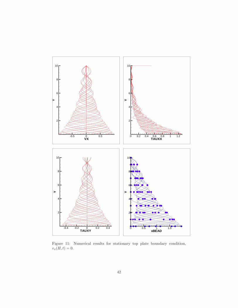
Stationary top plate. A closed-cell experimental setup is advantageous
in ensuring isolation of the sample and surrounding medium. Typical results
are shown in Fig. 11 when the top plate is kept at zero velocity vx(H, t) =
0. An interesting observation is that the velocity and stress profiles are very
similar to those obtained in the open-cell experiment. The main difference is the
much smaller range of motion exhibited by tracer beads when the top plate is
39

stationary by comparison to the open-cell experimental setup. If signal-to-noise
ratio of tracer bead positions becomes a concern at low strain thresholds, then
the open-cell setup is preferable.
5 Implications for inverse viscoelastic character-
ization
The theoretical results presented above provide new formulas in the linear finite
depth case, nonlinear UCM infinite depth case, and accurate numerical simula-
tion algorithms for the nonlinear finite depth case. Especially for experimental
measurements involving small samples, in which of necessity the depth is com-
parable to shear wavelengths, it is crucial to employ the finite depth formulas
deduced above rather than trying to fit to the infinite depth shear wave (28).
In subsequent work we shall use theses new tools to deduce viscoelastic param-
eters from bead tracking data in the presence of experimental noise. For this
paper we want to illustrate the effects that would arise from attempting to fit
measurements to inappropriate models even if there were no experimental error
whatsoever.
Instead of experimentally measured data we shall use bead positions gener-
ated from numerical simulations of a specific viscoelastic model. The goal then
is to infer linear and nonlinear viscoelastic properties from this “experimental
data set”, and to assess the magnitude of errors made as well as the dominant
source of error. Typically, least-squares procedures are employed to fit mea-
sured bead trajectories to theoretical formulas in order to obtain the complex
viscosity η∗(ω) (or complex shear modulus G∗(ω)). We adopt this procedure to
provide fair measurements of relative error.
If the same model is used both to generate the data and to carry out pa-
40

VX
Y
-0.5 0 0.5
2
4
6
8
10
TAUXX
Y
0 0.2 0.4 0.6 0.8 1 1.2
2
4
6
8
10
TAUXY
Y
-0.4 -0.2 0 0.2 0.4
2
4
6
8
10
xBEAD
Y
0 0.5 1 1.5
2
4
6
8
10
Figure 10: Numerical results for zero top shear stress, τxy(H, t) = 0, boundarycondition.
41
TAUXX
Y
0 0.2 0.4 0.6 0.8 1 1.2
2
4
6
8
10
TAUXY
Y
-0.4 -0.2 0 0.2 0.4
2
4
6
8
10
xBEAD
Y
0 0.5 1 1.5
2
4
6
8
10
VX
Y
-0.5 0 0.5
2
4
6
8
10
Figure 11: Numerical results for stationary top plate boundary condition,vx(H, t) = 0.
42

rameter fitting, then errors arise only from generation of model solutions or the
numerical least-squares procedure. We use this as a check to ensure the proce-
dure is accurate. Further errors in viscoelastic characterization arise if the data
is fit to a different model, e.g. if the Ferry infinite depth formulas are used to
characterize measurements made on a linear viscoelastic fluid in a finite-depth
cell. We present errors that arise from finite depth and nonlinear effects.
One unusual feature of these effects in the present non-dimensional formula-
tion is that there is no frequency dependence. This is because we have restricted
attention to a single-mode Maxwell type fluid.
5.1 Finite depth effects, linear viscoelastic model
Consider a viscoelastic fluid of depth H set into motion from rest by harmonic
oscillation of a bottom plate and upon which is placed a stationary top plate
(vH = 0). We wish to ascertain the error made in deriving viscoelastic param-
eters (η∗ or G∗) by fitting observed velocity profiles to the Ferry semi-infinite
solution (28), rather than the correct, finite-depth solution given in (36). Con-
sider the following best-case experimental scenario: measurements are made
at a large number of points, say m = 40, across the fluid depth and at small
time increments, Δt = 2π/n (e.g. n = 36 measurements per plate oscillation
period). The bead positions generated by the finite-depth solution (36) with
complex viscosity η∗H =η′H − η′′H are used to construct a least-squares fit to the
Ferry tracer bead position profile from whence another estimate of the complex
viscosity η∗F = η′F − iη′′F is obtained. The least squares sum is
S(η′F , η
′′F ) =
m∑j=1
n∑k=1
e2(yj , tn, δF , δH), δF =√i Re/η∗F , δH =
√i Re/η∗H ,
e(y, t,H, δF , δH) =∫ t
0
Im{eis
[e−δF y − sinh [δH(H − y)]
sinh (δHH)
]}ds (65)
43

The error function e(y, t,H, δF , δH) is presented in Fig. 12-14. As expected
when H increases the bead position error decreases (Fig. 12). Recall the link
between complex viscosity and Maxwell fluid parameters, η′ = ηp/(1 + λ2),
η′′ = ηpλ/(1 + λ2). We can increase the magnitude of the complex viscosity η∗
by increasing ηp and vary the phase of η∗ by varying λ but setting ηp = 1 + λ2
always. When the absolute value of the complex viscosity increases, the error
increases and furthermore becomes quasi-linear over the depth (Fig. 13). This
makes the identification of parameters ill conditioned. As the relaxation time
of the fluid λ becomes larger, the magnitude of the error remains essentially the
same Fig. 14. At small λ the identification of η∗ will be more difficult since
there are fewer oscillations of the shear wave within the depth H (Fig. 14).
0 1 2 3 4 5�3
�2
�1
0
1
2
y
e
0 1 2 3 4 5
�0.3
�0.2
�0.1
0.0
0.1
0.2
y
e
0 1 2 3 4 5
0.000
0.005
0.010
y
e
0 1 2 3 4 5
�0.0002
0.0000
0.0002
0.0004
0.0006
y
e
Figure 12: Error in bead positions between finite depth (36) and infinite depth(28) solutions (Re = 1, η′ = η′′ = 1). Top row H = 1, 5. Bottom row H =10, 15.
Snapshots of the error in identification of η∗ as presented above are useful,
44

0 1 2 3 4 5�6. � 10�10
�4. � 10�10
�2. � 10�10
0
2. � 10�10
y
e
0 1 2 3 4 5
�0.0015
�0.0010
�0.0005
0.0000
0.0005
0.0010
y
e
0 1 2 3 4 5
�0.05
0.00
0.05
0.10
0.15
0.20
y
e
0 1 2 3 4 5
�0.2
�0.1
0.0
0.1
0.2
0.3
0.4
y
e
Figure 13: As in Fig. 12. Constant H = 10. Top row η′ = η′′ = 0.05, 0.5.Bottom row η′ = η′′ = 5, 50.
but limited to single values of the complex viscosity. To obtain an overall picture
of the error made in identification of viscoelastic parameters we introduce the
complex mapping δF (δH), δF : C → C. This provides a measurement of the
error in fitting the true finite-depth solution to the semi-infinite Ferry solution,
and can also serve to correct the Ferry δF value. It is preferable to use δ rather
than the complex viscosity η∗ for two reasons: 1. δ = α+iβ is directly related to
experimentally measured quantities, the penetration depth 1/α and the shear
wavelength 2π/β; 2. The inversion η∗ = i Re/δ amplifies errors made when δ
is small and hence relatively small errors in δ give large changes in η∗.
A useful technique, common in the studies of conformal mappings, is to
present the δF (δH) mapping as a deformation of the αH = j Δα =constant and
βH = kΔβ =constant lines (j, k are integers and Δα, Δβ are the spacings with
which we sample δH space). If no error is made, an initially Cartesian (αH , βH)
45

0 1 2 3 4 5�2. � 10�7
�1. � 10�7
0
1. � 10�7
2. � 10�7
3. � 10�7
4. � 10�7
y
e
0 1 2 3 4 5
�5. � 10�7
�4. � 10�7
�3. � 10�7
�2. � 10�7
�1. � 10�7
0
y
e
0 1 2 3 4 5
�2. � 10�7
0
2. � 10�7
4. � 10�7
6. � 10�7
y
e
0 1 2 3 4 5
�4. � 10�7
�2. � 10�7
0
2. � 10�7
4. � 10�7
6. � 10�7
y
e
Figure 14: As in Fig. 12. Constant H = 10. Top row λ = 0.5, 1. Bottom rowλ = 5, 10. ηp = 1 + λ2 in all cases.
grid would be transformed into itself identically. The deviation from a Cartesian
map of the (αF , βF ) lines serves as an indication of the error made in using the
Ferry formula in the least squares fit to obtain the complex viscosity. To cover
as wide of range of values as possible the mappings are presented in logarithmic
coordinates. Typical results for H = 2, 5 are presented in figures 15, 16. The
purely viscous case α = β =√Re/2 is shown for reference. As expected errors
decrease as α increases - the shear wave is more attenuated and the boundary
condition at H has less influence. Note however that large values of α in bead
tracking experiments imply small bead displacements, which are difficult to
track. For smaller values of α the wavelength 2π/β is poorly identified. The
region of poor identification is smaller for smaller H as expected.
For certain regions it is even possible to use the δF (δH) mapping to correct
an erroneous estimate made by fitting to the Ferry semi-infinite solution! This
46

would be of interest in reinterpreting archived experimental data. Fig. 17 shows
a sequence of values obtained by fitting to the infinite depth formula and arrows
to the correct values (α, β) for that particular fluid.
It is apparent that very large errors are made when trying to deduce vis-
coelastic parameters from bead tracking data if the fit is carried out on the
infinite depth formula rather than the correct, finite depth model.
�1.0 �0.5 0.0 0.5 1.0�1.0
�0.5
0.0
0.5
1.0
lg�ΑH�
lg�ΒH�
Figure 15: The mapping δF (δH) for H = 2, Re = 1. The dot represents thepurely viscous case α = β =
√1/2. Large errors in viscoelastic characterization
arise for α < 10−0.25.
47

�1.0 �0.5 0.0 0.5 1.0�1.0
�0.5
0.0
0.5
1.0
lg�ΑH�
lg�ΒH�
Figure 16: As above for H = 5.
48

�0.5 �0.4 �0.3 �0.2 �0.1 0.0�1.0
�0.9
�0.8
�0.7
�0.6
�0.5
lg�ΑH�
lg�ΒH�
Figure 17: A plot of δF (δH) for H = 5, Re = 1 with arrows indicating how tocorrect erroneous (αF , βF ) values to the true viscoelastic fluid values (αH , βH),assuming linear viscoelasticity.
49

5.2 Onset on non-linear effects
We now consider how non-linear effects influence viscoelastic characterization.
Velocity profiles for a viscoelastic fluid placed between an oscillatory bottom
plate and a stationary top plate are generated by numerically solving system
(19). The numerically-generated velocity profiles contain non-linear effects from
(19). In order to quantify the onset of nonlinearity, we shall do a least-squares
fit of the numerical velocity data to the linear finite-depth formula (36) to obtain
the parameters (α, β) characterizing the shear wave. We present typical results
of the fitting procedure, highlighting the role of the bulk strain γ = 1/H and
Giesekus parameter a which controls shear thinning. At low values of γ (e.g.
γ < 0.1) the fitting procedure reproduces the numerical parameters used in the
simulations – this was used to validate the least squares algorithm used.
Moderate bulk strain, UCM fluid (γ = 0.25, a = 0). Results are pre-
sented in Fig. 18. At this moderate bulk strain value the fitting procedure
works very well for small Deborah numbers λ (λ ≤ 1). As the Deborah num-
ber is increased the results become markedly worse with errors in parameter
identification greater than 100% at λ = 16.
Large bulk strain, UCM fluid (γ = 0.5, a = 0). When the bulk strain
is large, the fitting procedure fails at all values of λ (Fig. 19).
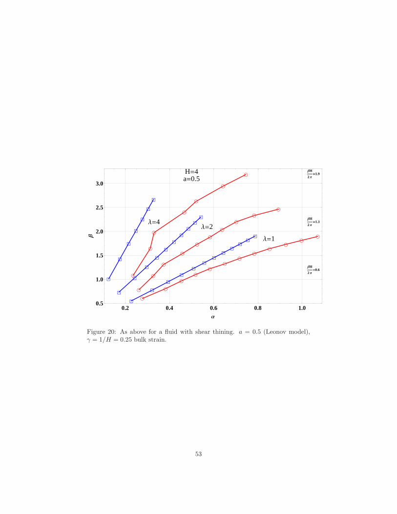
Moderate bulk strain, Giesekus fluid (γ = 0.25, a = 0.5). For moderate
bulk strains on a shear-thinning fluid we notice a systematic overestimate of α
even while β is captured rather well (Fig. 20). This is the expected behavior.
The penetration depth of wave propagating into the fluid 1/α is underestimated
by the linear viscoelastic model hence the α values are higher.
50

��
�� � � � � � � � �
��
� � � � � � � � � �
��
���� �
� �� �
��������
���
��������
������
��
�
�
�
�
�
�
�
�
�
�
�
�
�
�
Λ�1
Λ�2
Λ�4
Λ�16H�4a�0
ΒH
2�Π0.6
ΒH
2�Π1.3
ΒH
2�Π1.9
ΒH
2�Π2.6
ΒH
2�Π3.2
0.1 0.2 0.3 0.4 0.5 0.6 0.7 0.8
1
2
3
4
5
6
Α
Β
Figure 18: Comparison of shear wave identified by fitting to the linear, finitedepth formula (36), (circles) to parameters used to generate data numericall(squares). Bulk strain γ = 1/H = 0.25.
51

��
�� � � � � � � � �
� �����
��
����
��
����� �
����
����
�����
�
����
�
�
�
��������
�
�
�
���
��
���
Λ�1Λ�2
Λ�4
Λ�16
H�2a�0
ΒH
2�Π0.6
ΒH
2�Π1.3
ΒH
2�Π1.9
ΒH
2�Π2.6
ΒH
2�Π3.2
0.1 0.2 0.3 0.4 0.5 0.6 0.7 0.8
1
2
3
4
5
Α
Β
Figure 19: As above, but for higher strain γ = 1/H = 0.5. Nonlinear effects areso strong that fitting to linear model leads to meaningless results.
52
�
�
��
��������
�
��
��
��
��
��
�
�
�
�
�
������
�
�
�
�
��
��
��
�
�
�
�
�
�
�
�
�
�
�
�
�
�
Λ�1
Λ�2Λ�4
H�4a�0.5
ΒH
2�Π0.6
ΒH
2�Π1.3
ΒH
2�Π1.9
0.2 0.4 0.6 0.8 1.00.5
1.0
1.5
2.0
2.5
3.0
Α
Β
Figure 20: As above for a fluid with shear thining. a = 0.5 (Leonov model),γ = 1/H = 0.25 bulk strain.
53

6 Conclusions
For purposes of inverse characterization experiments in low volume samples of
biological fluids (such as pulmonary airway surface liquids, our motivation for
this work), we have extended the Ferry shear wave analysis to include finite-
depth within linear viscoelasticity, and then to include nonlinearity with con-
stitutive laws of Maxwell type. The linear models are exactly solvable, allowing
for an explicit measure of errors in the inverse characterization of a known vis-
coelastic material due solely to finite depth effects. At frequencies and bulk
strains typical for conditions encountered by the airway surface liquid in the
lung, errors in the recovery of storage and loss moduli are enormous when fit-
ting to inappropriate theoretical models. For viscoelastic fluids that can safely
be assumed to be behave linearly, fitting to the newly derived finite depth for-
mula (36), which accounts for counterpropagating shear waves and stress modes,
is shown to work well. If the fluid behaves nonlinearly as controlled bulk strain
from the driven plate is ramped up, either due to convective nonlinearity or
shear thinning, then inverse recovery of viscoelastic parameters by fitting to the
extended finite-depth linear formulas induce significant errors.
These modeling tools have been developed in context with a new device, a
micro, parallel-plate rheometer, which allows both types of velocity controls on
the opposing flat interface to the driven plate. The present paper has illustrated
recovery of linear and nonlinear viscoelastic parameters as well as predictions
of onset of nonlinear effects at threshold values of the imposed strain from
the driven plate. In a future article, we will apply these modeling tools to
experiments on biological liquids.
Acknowledgements. This work originated with and has benefited from dis-
cussions with colleagues involved in the University of North Carolina Virtual
Lung Project. The research effort was sponsored by NIH grant R01-HL077546-
54

01A2, NSF Research Training Grant DMS-0502266, NSF-DMS 0604891, and
ARO 47089-MS-SR.
References
[1] John D. Ferry, Studies of the Mechanical Properties of Substances of High
Molecular Weight I. A Photoelastic Method for Study of Transverse Vibra-
tions in Gels, Rev. Sci. Inst., 12, 79-82, (1941)
[2] John D. Ferry, W.M. Sawyer, and J. N. Ashworth, Behavior of Concentrated
Polymer Solutions under Periodic Stresses, J. Polym. Sci. 2:593-611, (1947)
[3] F.T. Adler, W.M. Sawyer, John D. Ferry, Propagation of transverse waves
in viscoelastic media, J. Appl. Phys., 20, 1036-1041 (1949)
[4] G.B. Thurston, J.L. Schrag, Shear wave propagation in a Birefringent vis-
coelastic medium, J. Appl. Phys. 35, 144, 1964.
[5] Hermann Schlichting, Boundary layer theory, McGraw-Hill, New York,
1960.
[6] J.D. Ferry, Viscoelastic properties of polymers, John Wiley, New York, 1980.
[7] R.B. Bird, R.C. Armstrong, O. Hassager, Dynamics of Polymeric Liquids,
Fluid Mechanics, Vol. 1, Wiley, New York, 1987.
[8] D. B. Hill, B. Lindley, M.G. Forest, S.M. Mitran, Microrheology of DNA
solutions from bead tracking of shear waves, UNC preprint, 2007.
[9] D.B. Hill, R. Superfine, Microbead rheology, (In preparation).
[10] H. Matsui, S. Randell, S. Peretti, C. W. Davis, and R. C. Boucher, Coor-
dinated clearance of periciliary liquid and mucus from airway surfaces, J.
Clin. Invest., 102(6), 1125-1131, 1998.
55

[11] S. M. Mitran, Highly accurate solutions of the non-linear one-dimensional
viscoelastic shear wave problem for Giesekus type fluids, (in preparation)
[12] R.G. Larson, Constitutive Equations for Polymer Melts and Solutions, But-
terworths, Guildford, UK, 1988.
[13] J.C. Crocker, M.T. Valentine, E.R. Weeks, T. Gisler, P.D. Kaplan, A.G.
Yodh, and D.A. Wietz, Phys. Rev. Lett. 85, 888, 2000.
[14] M. Gregory Forest, Qi Wang, Dynamics of slender viscoelastic free jets,
SIAM J. Appl. Math., 54(4), 996-1032,(1994).
[15] R. J. LeVeque, Wave propagation algorithms for multi-dimensional hyper-
bolic systems, J. Comp. Phys., 131, 327-353, 1997.
[16] S. Mitran, BEARCLAW - A software frame-
work multiphysics numerical simulation,
http://www.amath.unc.edu/Faculty/mitran/bearclaw.html.
[17] R. J. LeVeque, CLAWPACK - Conservation Law Package,
http://www.amath.washington.edu/~claw.
[18] D.E. Knuth, Literate Programming, Stanford, CSLI Lecture Notes, no. 27,
1992.
[19] http://www.amath.unc.edu/Faculty/mitran/research/viscelas/shear1d.xhtml
56