Entropy 2008, 10, 477-492; DOI: 10.3390/e10040477

entropy ISSN 1099-4300

www.mdpi.com/journal/entropy Article

Extended Thermodynamics: a Theory of Symmetric Hyperbolic Field Equations

Ingo Müller

Technical University Berlin, Berlin, Germany E-mail: Ingo.Mueller@alumni.tu-berlin.de

Received: 31 July 2008; in revised form: 9 September 2008 / Accepted: 22 September 2008 / Published: 15 October 2008

Abstract: Extended thermodynamics is based on a set of equations of balance which are supplemented by local and instantaneous constitutive equations so that the field equations are quasi-linear first order differential equations. If the constitutive functions are subject to the requirements of the entropy principle, one may write them in symmetric hyperbolic form by a suitable choice of fields. The kinetic theory of gases, or the moment theories based on the Boltzmann equation provide an explicit example for extended thermodynamics. The theory proves its usefulness and practicality in the successful treatment of light scattering in rarefied gases. This presentation is based upon the book [1] of which the author of this paper is a co-author. For more details about the motivation and exploitation of the basic principles the interested reader is referred to that reference. It would seem that extended thermodynamics is worthy of the attention of mathematicians. It may offer them a non-trivial field of study concerning hyperbolic equations, if ever they get tired of the Burgers equation. Physicists may prefer to appreciate the success of extended thermodynamics in light scattering and to work on the open problems concerning the modification of the Navier-Stokes-Fourier theory in rarefied gases as predicted by extended thermodynamics of 13, 14, and more moments. Keywords: extended thermodynamics, entropy

1. Formal Structure The objective of extended thermodynamics is the determination of n fields, synthetically denoted by

),( txu dα (α=1,2,…n) and called densities. The argument xd denotes the spatial coordinates of an event

OPEN ACCESS

Entropy 2008, 10

478

and t is its time. Invariably, the first five of these fields are chosen as the densities of mass, momentum and energy – and that is all in ordinary thermodynamics. But in extended thermodynamics the number of fields is extended (sic!) and it may contain the stress, the heat flux and more, see below.

For the determination of the fields ),( txu dα we need n field equations, and these are based upon n

equations of balance. Summation is implied over repeated indices, whether Greek or Latin.

ααα Π=

∂∂

+∂∂

d

d

xF

tu

α = (1,2,…n). (1.1) dFα (d = 1,2,3) are called fluxes, and αΠ are called productions.

If the first five equations (1.1) represent the conservation laws of mass, momentum, and energy, the first five productions αΠ (α=1,…5) vanish. And all productions vanish in equilibrium.

In order to obtain field equations for the densities αu , the equations of balance must be

supplemented by constitutive equations. Such constitutive equations relate the fluxes and productions to the densities in a manner characteristic for the material. In extended thermodynamics the constitutive relations have the forms

)(ˆβαα uFF dd = and )(ˆ

βαα uΠ=Π (1.2)

so that the fluxes dFα and productions αΠ at a point and a time depend only on the densities αu at that

point and time. We may say that the constitutive equations are local in space-time. Thus no gradients or time derivatives occur among the variables in the constitutive equations. In particular; there is no temperature gradient. And yet heat conduction is accounted for, because the heat flux is counted among the variables.

If the constitutive functions dFαˆ and αΠ̂ were known explicitly, we could eliminate dFα and

αΠ between the equations of balance and the constitutive relations and obtain explicit field equations for the αu ´s. They form a quasi-linear system of partial differential equations of first order. Every

solution of this system is called a thermodynamic process.

2. Symmetric hyperbolic systems In reality, of course, the constitutive functions are not known, and it is the task of the constitutive

theory to determine those functions or, at least, to reduce their generality. The tools of the constitutive theory are certain universal physical principles which represent expectations based on experience. The main principles are:

● entropy inequality, ● requirement of concavity, ● principle of relativity.

The first two of these combined represent the entropy principle. The entropy inequality is an additional balance law which we write as

0≥Σ=∂∂

+∂∂

d

d

xh

th , for all thermodynamic processes. (2.1)

h is the entropy density and hd is the entropy flux. Σ is the entropy production, assumed non-negative for all thermodynamic processes. All three of those quantities are constitutive quantities so that in extended thermodynamics we have

Entropy 2008, 10

479

)(ˆ),(ˆ),(ˆ βββ uuhhuhh dd Σ=Σ== . (2.2) The requirement of concavity demands that h be a concave function of βu , i.e.

βα uuh∂∂

∂ 2

- negative definite. (2.3)

The principle of relativity states that the field equations and the entropy inequality have the same forms in all Galilei frames. In relativistic thermodynamics we require the same invariance under Lorentz transformations.

We defer the consideration of the principle of relativity and proceed with the exploitation of the entropy principle. The key to the exploitation of the entropy inequality lies in the observation that the inequality need not hold for all fields αu ; rather it must hold for thermodynamic processes, i.e.

solutions of the field equations. In a manner of speaking the field equations provide constraints for the fields αu that must satisfy the entropy inequality. A lemma by Liu [2] proves that it is possible to use Lagrange multipliers βΛ , -- functions of αu

- to eliminate the constraints. Indeed, the new inequality

0≥⎟⎟⎠

⎞⎜⎜⎝

⎛Π−

∂∂

+∂∂

Λ−∂∂

+∂∂

ααα

α d

d

d

d

xh

tu

xh

th

must hold for all fields ),( txu dα . In particular this inequality must hold for arbitrary derivatives

tu∂∂ α and dx

u∂∂ α at one event, and this implies

αα uh dd Λ= , dd Fh ααdd Λ= and 0≥ΣΛ αα . (2.4)

From (2.4)1 we conclude that

βαβ

α

uuh

u ∂∂∂

=∂Λ∂ 2

is negative definite because of the concavity of h as a function of αu . Therefore there is a one-to-one correspondence between the densities αu and the Lagrange multipliers βΛ . It is thus possible to make a change of variables αα Λ⇔u . If this is done, the two equations (2.4)1,2 may be written in the form

αα Λ=′ dd uh , αα Λ=′ dd dd Fh , (2.5) where ααuhh Λ+−=′ and aaa Fhh ααΛ+−=′ are called scalar and vector potentials respectively, because their derivatives with respect to αΛ are the densities and the fluxes. Therefore in the new

variables the system of field equations reads

αβ

βα

β

βα

Π=∂

Λ∂

Λ∂Λ∂′∂

+∂

Λ∂

Λ∂Λ∂′∂

d

d

xh

th 22

, (α=1,2,…n). (2.6)

All four matrices in this system are obviously symmetric and the first one is negative definite. This follows from the concavity of the entropy density in terms of the densities αu , since

ααuhh Λ+−=′ defines a Legendre transformation associated to the map αα Λ⇔u . Such a Legendre transformation preserves concavity so that h′ is a concave function of αΛ . Therefore the system of

field equations – written in terms of Lagrange multipliers – is a symmetric hyperbolic system. Hyperbolicity guarantees finite speeds of propagation and symmetric hyperbolic systems have

convenient and desirable mathematical properties, namely well-posedness of Cauchy problems, i.e. existence, uniqueness, and continuous dependence on the data. The desire for finite speeds of

Entropy 2008, 10

480

propagation was the primary original incentive for the formulation of extended thermodynamics by Müller [3].

The residual inequality (2.4)3 is due entirely to the production terms in the field equations; recall that the first five productions are zero. Since αΠ may be considered as a function of the Lagrange

multipliers βΛ , it follows from the inequality that in equilibrium – defined by 0E=Πα -- all βΛ

(β=6,7,…n) are equal to zero 0

E=Λβ , (β=6,7,…n) . (2.7)

The residual inequality is a sum of products of the productions and the Lagrange multipliers. In the jargon of ordinary – non-extended – thermodynamics we may consider these quantities as thermodynamic forces and fluxes. And in a linear theory the forces are linear functions of the fluxes, so that we may write

∑=

=n

L6β

βαβα ΛΠ , (α=6,7,…n). (2.8)

3. Characteristic speeds and pulse speed

A wave is a moving surface, represented mathematically by the equation 0),( =txdϕ ,

which defines the wave front. The unit normal nd and the normal speed V are given by

ϕ

ϕ

grad

dd xn ∂

∂

= and ϕ

ϕ

gradtV ∂

∂

−= . (3.1)

In the simple case considered here the wave front separates the constant and homogeneous fields ),( txd

αΛ in front of the wave from the perturbed fields behind it. In the case of weak waves – or

acceleration waves. In fluid mechanics weak waves have a continuous velocity across the front but a jump of acceleration; hence the name acceleration wave. The fields are continuous across the front, but the gradients have a jump and, obviously, that jump points in the direction of the normal. Therefore

[ ] 0=Λα and hence αα Jn

xd

d =⎥⎦⎤

⎢⎣⎡∂Λ∂

and αα VJt

−=⎥⎦⎤

⎢⎣⎡∂Λ∂

, (3.2)

where a square bracket [a] denotes the difference of a generic quantity a in front of the wave and behind it. αJ (α=1,2,…n) are called the amplitudes of the acceleration wave.

In our case the speeds and amplitudes are given by the field equations (2.6) as solutions of the homogeneous linear algebraic system

022

=⎟⎟⎠

⎞⎜⎜⎝

⎛

Λ∂Λ∂′∂

−Λ∂Λ∂′∂

ββαβα

JnhVh dd

. (3.3)

Thus the possible wave speeds in the direction nd are the solutions of the characteristic equation

det 022

=⎟⎟⎠

⎞⎜⎜⎝

⎛

Λ∂Λ∂′∂

−Λ∂Λ∂′∂ d

d

nhVh

βαβα

. (3.4)

We obtain n speeds and they are called characteristic speeds. The fastest one of these is called the pulse speed. All speeds are real and finite as a consequence of the symmetric hyperbolic character of the field equations. By (3.3) the amplitudes Jβ are right eigen-vectors of the matrix of the linear system.

Entropy 2008, 10

481

4. Growth and decay of acceleration waves The solutions of non-linear hyperbolic equations have a tendency to develop singular derivatives

even when the initial data are smooth. Thus, jumps – or shocks – may appear. However, dissipation – represented by the productions in the equations (2.6) – can put a check on this tendency.

The conditions on initial data and on the dissipative terms which need to be satisfied to guarantee smooth solutions for all times are unknown. All we have is a sufficient condition for smoothness by Kawashima [4]. However, the treatment of acceleration waves gives a good intuitive understanding of what is involved.

It is possible to determine the rate of change tJδδ of the amplitude of acceleration waves. This was

first done by W.A.Green [5] but the most elegant derivation and result is due to Boillat [6]. We shall restrict the attention to the case that the wave propagates into a region of equilibrium with constant and homogeneous fields. In that case Boillat´s result reduces to a Bernoulli equation with constant coefficients

02 =∂Π∂

−Λ∂∂

− Jdu

lJdVtJ

ba

ββ

ααβ

βδδ . (4.1)

lα and dα are the left and right eigen-values of the matrix of the linear system (3.3). The coefficient a, indicated in (4.1), represents non-linearity of the system, namely the dependence of the wave speed upon the value of the fields αΛ . The coefficient b represents dissipation, because it depends on the

productions in the field equations. The solution of (4.1) reads

)1()0(1)0()(

−−= −

−

btba

bt

eJeJtJ . (4.2)

If the system were linear, i.e. a=0, there would be exponential decay, of course. But even for 0≠a there may be decay unless the initial amplitude is too big. If that amplitude is big enough, J(t)

becomes singular at some time. For an acceleration wave this means that the amplitude of acceleration becomes infinite, so that the velocity has a jump; a shock wave appears, a discontinuity of velocity.

Experiments show that discontinuities do not exist. Natura non fecit saltus! If a mathematical theory predicts discontinuities, e.g. jumps of velocity in a shock wave, it is a sure sign that the theory is deficient and additional fields are required to resolve the discontinuity into a steep but smooth structure. Extended thermodynamics of moments shows the way in which this may be done, cf. [1]. Parabolisation of the field equations, -- euphemistically called regularization by mathematicians --, is not the correct way. 5. An example. Extended thermodynamics of moments

5.1. Pulse speeds

The kinetic theory of gases is based on the Boltzmann equation for the distribution function

),,( tcxf dd which determines the number density of atoms – of mass μ – with the velocity cd at the point xd and time t. The moments of the distribution function are

Entropy 2008, 10

482

∫= cfcccull iiiiii d...

2121 ..... μ , (5.1)

So that u, ui, and uii are the densities of mass, momentum and energy of the gas. The moments obey equations of balance of the form (1.1), viz.

l

lliiid

diiiiii

xu

tu

.........

21

2121 Π=∂

∂+

∂

∂, (l=0,1,2,…N). (5.2)

For u, ui, and uii the productions Π, Π i, and Π ii vanish because of the conservation of mass, momentum and energy in atomic collisions. Since each index may assume the values 1,2,3, there are

)3)(2)(1(61 +++= NNNn equations.

These equations fit into the formal framework of extended thermodynamics, but they are simpler Indeed, on the left hand side there is only one flux, namely diii N

u ...21-- the last one – which is not

explicitly related to liiiu ...21(l=0,1,2,…N). Therefore the results of Sections 2 and 3 may be carried over

to the present case, in particular the exploitation of the entropy inequality. In the kinetic theory of gases that inequality assumes the form

( ) ( ).0

dlndln ee≥

∂

−∂+

∂

−∂ ∫∫a

Yf

aYf

x

cfck

t

cfk (5.3)

e is the Euler number and 1/Y is the smallest cell of the phase space spanned by xa and ca . The exploitation makes use of the Lagrange multipliers

liii .....21Λ (l=0,1,2,…N) and the moment

character of the densities and fluxes implies that the distribution function has the form ( )

ll iiiiiik cccYf ...exp2121 ...

1 μΛ−= (5.4)

so that the scalar and vector potential may be written as ( )∫ Λ−−=′ cccckYh

ll iiiiiik d...exp2121 ...

1 μ and ( )∫ Λ−−=′ ccccckYhll iiiiiika

a d...exp2121 ...

1 μ (5.5)

Insertion into the characteristic equation (3.4) for the calculation of the wave speeds gives ( ) 0d...)(det E21

=−∫ cfcccVncliiiaa (5.6)

provided that the wave propagates into a region of equilibrium. fE is the Maxwell distribution. Thus the calculation of characteristic speeds and, in particular, the pulse speed, requires no more

than simple quadratures and the solution of an nth order algebraic equation. It is true that the dimension of the determinant in (5.6) increases rapidly with N: For N = 10 we have 286 rows and columns, while for N = 40 we have 12341 of them. But then, the calculation of the elements of the determinant and the determination of the pulse speed Vmax may be programmed into the computer and W.Weiss [7] has the values ready for any reasonable N at the touch of a button, cf. Figure 1. We recognize from the figure that the pulse speed goes up with increasing N and it never stops. Indeed, according to Boillat & Ruggeri [8] there exists a lower bound for Vmax which tends to infinity for .∞→N

The fact that Vmax is unbounded in a non-relativistic moment theory represents something of an anticlimax for extended thermodynamics, because that theory started out originally as an effort to find a finite speed of heat conduction. But it does not matter! Indeed by the time the conclusion was reached, extended thermodynamics had long outgrown its original motif. Anyway the problem lies with the kinetic theory rather than with extended thermodynamics. After all, infinite speeds of atoms are permitted in the non-relativistic kinetic theory and in the Maxwell distribution. For that reason the moments are integrals over the whole range of velocities from -∞ to +∞. It had become a predictive theory which is needed when steep gradients and rapid changes occur as they do in light scattering. Let us consider that:

Entropy 2008, 10

483

5.2. Field equations for moments Once the distribution function is known in terms of Lagrange multipliers, cf. (5.4), it is possible --

in principle – to change back from the Lagrange multipliers liii ...21

Λ to the moments liiiu ...21 by inverting

the relation

Figure 1. Pulse speeds referred to the normal sound speed. Table and crosses: Calculations by Weiss Circles: Lower bound )( 2

156 −N by Boillat and Ruggeri.

( )∫ Λ−= cccc Ycccullll iiiiiikiiiiii d...exp...

21212121 ...1

..... μμ . (5.7)

Once this is done, we may determine the last flux

diii Nu ...21

= ( )∫ Λ− cccc Ycccclll iiiiiikaiii d...exp...

212121 ...1 μμ (5.8)

in terms of the densities liiiu ...21(l=0,1,2,…N). Also the productions may thus be calculated after we

choose an appropriate model for the atomic interaction, e.g. the model of Maxwellian molecules. In reality the calculations of the flux diii N

u ...21 and of the non-zero productions

liii ...21Π (l=6,7,…N)

require somewhat precarious approximations, since integrals of the type occurring in (5.8) cannot be solved analytically. Those approximations deserve further study but when everything is said and done, one arrives at explicit field equations, e.g. those of Figure 2, which are valid for N=3 so that there are 20 individual equations. A fully satisfactory theory of extended thermodynamics, which does not need the precarious approximation, is presented in [9]. The equations written in the figure are linearized and the canonical notation has been introduced like ρ for the mass density u, ρvi for the momentum density ui , 3/2ρk/μT for the energy density 1/2uii, t<ij> for the deviatoric stress and qi for the heat flux. The moment u<ijk> has no conventional name, - other than trace-free third moment – because it does not enter the conventional equations of balance of mass, momentum, and energy. And yet, it does have to satisfy an explicit field equation.

The figure shows the same set of 20 equations four times so as to make it possible to point out special cases within the different frames. ● On the upper left side we see the equations for the Euler fluid, which is entirely free of

dissipation and thus without shear stresses and heat flux. ● The upper right box contains the Navier-Stokes-Fourier equations with the stress proportional to

the velocity gradient and the heat flux proportional to the temperature gradient. This set

Entropy 2008, 10

484

identifies the only unspecified coefficient τ as related to the shear viscosity η. We have Tk

μτρη 34= so that η grows linearly with T as is expected for Maxwellian molecules.

● In the fifth equation of the third set I have highlighted the Cattaneo equation. Cattaneo [10] was a forerunner of extended thermodynamics, who provided a modification on the Fourier law on the grounds of kinetic arguments by adding a term with the rate of the heat flux to it.

● The fourth box exhibits the 13-moment equations. These were formulated by Grad [11] as an example for his moment method for the approximate determination of the consequences of the Boltzmann equation. They are the most popular equations of extended thermodyna-mics, because they contain only the moments ρ, ρvi, T, t<ij> and qi known from ordinary thermodynamics.

Figure 2. Each one of the four groups represent the field equations of extended thermodynamics for N=3. Top left: Euler equations. Top right: Navier Stokes equations. Bottom left: Cattaneo equations. Bottom right: Grad´s thirteen moment equations.

For an interpretation we may rely on the upper right box in Figure 2, the one that emphasizes the

Navier-Stokes-Fourier theory. Inspection shows that some specific terms are left out of that theory, namely:

tt ij

∂

∂ >< and t

qi

∂∂

and jij

xt∂

∂ >< and ki

xq

∂∂

. (5.9)

Entropy 2008, 10

485

For rapid rates and steep gradients we may suspect that these terms do count and indeed they do, and we must go to the full set of 20 equations, or to equations with even more moments.. Since rapid rates and steep gradients are measured in terms of mean times of free flight and mean free paths, we may suspect that extended thermodynamics becomes necessary for rarefied gases.

5.3. Light scattering in gases as an example of extended thermodynamics of moments

The random thermal motion of the atoms or molecules of a gas disturb the equilibrium of a gas and

generate tiny and short lived compressions and expansions, i.e. fluctuations of density. These make the dielectric constant of the gas fluctuate, because it depends on the density. By Maxwell´s equations the fluctuations cause a light wave to be scattered sideways, cf. Figure 3a. Most of the scattered light has the frequency ω(i) of the incident mono-chromatic light, but neighbouring frequencies ω are also present in the scattering spectrum S(ω). Typically the measured spectrum – scattered in a gas and passed through an interferometer to a photo-multiplier – exhibits three well-developed peaks, if the gas is normally dense. In a rarefied gas measurements show a flatter curve with lateral shoulders, cf. Figure 3b.

Figure 3. On light scattering: a). Light scattering, schematic; b). Scattering spectrum in a dense gas and in a rarefied gas Dots: Measurements in a rarefied gas. Lines: Calculation by Navier-Stokes-Fourier theory.

a b The light scattering spectrum may also be calculated from the field equations fort he gas, e.g. the

Navier-Stokes-Fourier equations. The key to the calculation is the Onsager hypothesis by which the spatial Fourier components of the fields are the same functions of time as the mean regression of a fluctuation. For dense gases the measured and calculated scattering spectra agree perfectly well. This fact supports the Onsager hypothesis. For a rarefied gas, however, the agreement is bad, cf. Figure3b. Therefore we may conclude that the discrepancy is due to the Navier-Stokes-Fourier theory which, indeed, is expected to fail in a rarefied gas, according to the considerations of Section 5.2.

So, this is a case where extended thermodynamics can prove its usefulness and practicality. Weiss [7] has applied the linearized field equations of 20, 35, 56, and 84 moments to the problem and has calculated the scattering spectra of Figure 4 (top) for small pressures for which the experimental dots of Figure 3b were obtained. Inspection shows that the theories differ among themselves and that none

Entropy 2008, 10

486

of them fits the experimental points well. Nor can we adjust parameters to obtain a better fit, because there are no adjustable parameters of the usual type in extended thermodynamics. The only available parameter is the number of moments and moment equations. Therefore Weiss went ahead to 120 through 286 moments and obtained convergence as well as a perfect fit, cf. Figure 4 (bottom).

That result might be called satisfactory, amazing and disappointing at the same time: ● Satisfaction comes from the fact that extended thermodynamics combined with the Onsager

hypothesis is capable of representing light scattering satisfactorily in rarefied gases. ● The amazing feature is the convergence of the light scattering spectra at some finite number of

moments. More moments will not appreciably change the calculated curves. ● Disappointment stems from the large number of moments needed to achieve convergence. We

might have hoped that 13 or, perhaps 14 or 20 moments could give good results. That would have given us a manageable system of equations. Instead we need 120 of them, - at least for the small pressures to which the curves of Figure 4 refer.

Figure 4. Light scattering spectra in a moderately rarefied gas. Dots represent measurements. Top: Extended thermodynamics of N=20, 35, 56, 84 moments. Bottom: Extended thermodynamics of N =120, 165, 220, 286.

And yet, the results for light scattering represent the claim to fame of extended thermo-dynamics.

Indeed, the convergence put in evidence by the plots of Figure 4 permits us to conclude that extended thermodynamics determines its own range of applicability without any reference to experiments. This is something that is often said to be impossible. Yet in extended thermodynamics it is possible because it is not a single theory; it is a theory of theories, one each for a given number of moments. So, if – after an increase of that number – we obtain the same function S(ω) in some norm, we have reached convergence and may fully trust the theory and predict the light spectrum, without making a single experiment.

Entropy 2008, 10

487

5.4. Shock waves and shock structures Shock waves, or rather shock structures, offer a natural field of application for extended

thermodynamics, because they are steep. And it is known that the Navier-Stokes-Fourier theory cannot satisfactorily describe them, at least not for high Mach numbers of the shock. A good thing in the treatment of shock structures is that – even for many moments – boundary conditions are no problem. Indeed, we know their values far in front and far behind the shocks; they are equilibria.

And yet, the calculations are infinitely more difficult than those for light scattering, because we need the full non-linear equations, of course. Therefore the application of extended thermodynamics to shock waves has been limited to a moderate number of moments. The results are better than those of the Navier-Stokes-Fourier theory but they are limited – at this time – to Mach numbers less than 3 which is not enough. For an exposition of what has been achieved I refer to [1] and [12].

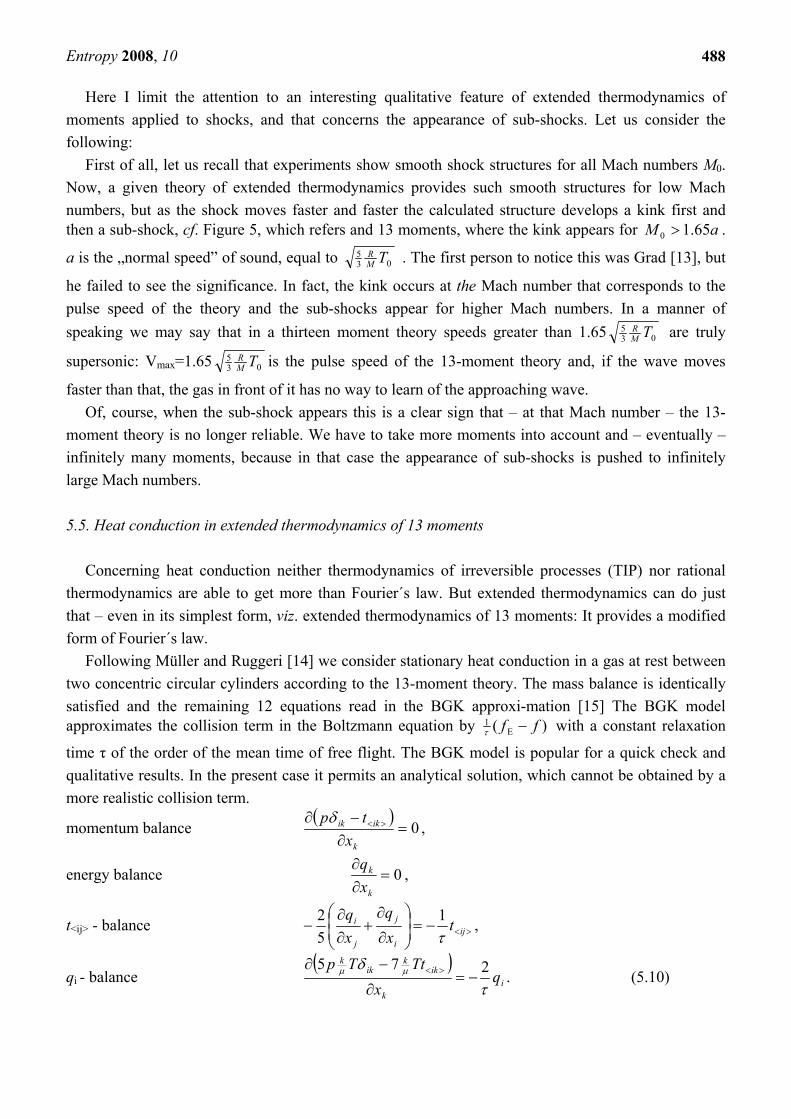
Figure 5. Shock structures of velocity and temperature for 13 moments. a. M0=1.5, b. M0=1.65, c. M0=2.0.

b.

c.

a.

Entropy 2008, 10

488

Here I limit the attention to an interesting qualitative feature of extended thermodynamics of moments applied to shocks, and that concerns the appearance of sub-shocks. Let us consider the following:

First of all, let us recall that experiments show smooth shock structures for all Mach numbers M0. Now, a given theory of extended thermodynamics provides such smooth structures for low Mach numbers, but as the shock moves faster and faster the calculated structure develops a kink first and then a sub-shock, cf. Figure 5, which refers and 13 moments, where the kink appears for aM 65.10 > .

a is the „normal speed” of sound, equal to 035 TM

R . The first person to notice this was Grad [13], but

he failed to see the significance. In fact, the kink occurs at the Mach number that corresponds to the pulse speed of the theory and the sub-shocks appear for higher Mach numbers. In a manner of speaking we may say that in a thirteen moment theory speeds greater than 1.65 03

5 TMR are truly

supersonic: Vmax=1.65 035 TM

R is the pulse speed of the 13-moment theory and, if the wave moves

faster than that, the gas in front of it has no way to learn of the approaching wave. Of, course, when the sub-shock appears this is a clear sign that – at that Mach number – the 13-

moment theory is no longer reliable. We have to take more moments into account and – eventually – infinitely many moments, because in that case the appearance of sub-shocks is pushed to infinitely large Mach numbers.

5.5. Heat conduction in extended thermodynamics of 13 moments

Concerning heat conduction neither thermodynamics of irreversible processes (TIP) nor rational

thermodynamics are able to get more than Fourier´s law. But extended thermodynamics can do just that – even in its simplest form, viz. extended thermodynamics of 13 moments: It provides a modified form of Fourier´s law.

Following Müller and Ruggeri [14] we consider stationary heat conduction in a gas at rest between two concentric circular cylinders according to the 13-moment theory. The mass balance is identically satisfied and the remaining 12 equations read in the BGK approxi-mation [15] The BGK model approximates the collision term in the Boltzmann equation by )( E

1 ff −τ with a constant relaxation

time τ of the order of the mean time of free flight. The BGK model is popular for a quick check and qualitative results. In the present case it permits an analytical solution, which cannot be obtained by a more realistic collision term.

momentum balance ( )

0=∂−∂ ><

k

ikik

xtpδ

,

energy balance 0=∂∂

k

k

xq

,

t<ij> - balance ><−=⎟⎟⎠

⎞⎜⎜⎝

⎛

∂

∂+

∂∂

− iji

j

j

i txq

xq

τ1

52 ,

qi - balance ( )

ik

ikk

ikk

qx

TtTpτ

δ μμ 275−=

∂

−∂ >< . (5.10)

Entropy 2008, 10

489

In the physical cylindrical coordinates appropriate for the problem the solution can eysily be found. It reads

p – homogeneous ⎥⎥⎥

⎦

⎤

⎢⎢⎢

⎣

⎡−><

0000000

21

21

54

54

rc

rc

ijt ττ

⎥⎥⎥

⎦

⎤

⎢⎢⎢

⎣

⎡

>=<00

1rc

iq ⎟⎟⎠

⎞⎜⎜⎝

⎛+−= 2

11

2 2528ln

5rc

ppccTk

ττμ

. (5.11)

c1 and c2 are constants of integration to be determined by boundary conditions. From all of this, -- in particular (5.10)4 –we conclude that qi is no longer solely determined by the

temperature gradient as it is by Fourier´s law; rather there is an additional term due to the deviatoric stress. And that term modifies the temperature field as shown in (5.11)4: unlike the Fourier theory T(r) is no longer determined by lnr. Figure 6 shows a comparison of the temperature fields according to the present theory and the Fourier case. The pressure is chosen as 2m

N210 and the boundary conditions are

those indicated in the Figure

Figure 6. Temperature field between coaxial cylinders. Boundary values.

As expected, the difference of the two solutions becomes noticeable where the temperature field is

steep. Note also that the Fourier solution becomes singular for 0int →r , but the 13-moment solution

remains finite. Additional remarkable phenomena are implied by extended thermodynamics when we let the two

co-axial cylinders be at rest on a turntable, i.e. in a non-inertial frame. According to the Navier-Stokes-Fourier theory the gas will rotate rigidly along with the cylinders, but in a 13-moment theory this is impossible, when heat is conducted between the cylinders, cf. Barbera and Müller [25].

Furthermore the continuity of the entropy flux at a thermometric wall does no longer imply continuity of T, cf. [14], [17]. This fact gives rise to the possibility to distinguish between a kinetic temperature – a measure of the atomic speeds – and the thermodynamic temperature – a continuous quantity at the wall of a thermometer.

Entropy 2008, 10

490

5.6. Boundary values for higher moments In extended thermodynamics of more than 13 moments a problem arises as to the boundary values

of higher moments: they must be prescribed in order to solve the equations, but in the laboratory it is impossible to prescribe and control them. That problem is unsolved. Barbera, Müller, Reitebuch and Zhao [18] have suggested that the uncontrollable boundary values fluctuate with the thermal motion and that the gas reacts to the mean values. That looks like a hopeful avenue but further tests of the proposition are necessary.

6. On the origin and development of extended thermodynamics

When extended thermodynamics started with the work of Müller [3], [18] its sole and – from the

present point of view – rather naïve objective was the resolution of the so-called paradoxa of heat conduction and shear wave propagation: The Navier-Stokes-Fourier theory has a parabolic structure and it predicts infinite pulse speeds. Working within the then prevailing theory of Thermodynamics of Irreversible Processes (TIP), Müller allowed the local entropy to depend on on the heat flux and the viscous stress. Also he assumed the entropy flux to be given by a generic constitutive equation rather than being determined universally by the ratio of heat flux and temperature, cf. [20]. This theory led to hyperbolic equations for temperature and shear velocities.

That early type of extended thermodynamics profited from the contact with the kinetic theory of gases – still in [19] – particularly with the moment method by Grad [11]. Later the connection between extended thermodynamics and the kinetic theory of gases became really close in the work [21] by Liu and Müller, where Lagrange multipliers were used for the exploitation of the entropy inequality. In this manner extended thermodynamics assumed a neat systematic form, albeit only for 13 or 14 moments.

Yet in this shape the theory was prepared to be joined to the mathematical theory of hyperbol--ic systems. Ruggeri and Strumia [22] recognized that the Lagrange multipliers – their main field – were privileged as a variable field and, if they are chosen, they make the field equations symmetric hyperbolic. With this observation it became possible to reveal the formal structure of extended thermodynamics which I have described in Sections 1 and 2 above. That formal structure – applied to moments was refined and extended by Boillat and Ruggeri [23], [24]. In the end the authors proved – in [8] – that the pulse speed, though finite for any finite number of moments, tends to infinity for infinitely many moments, at least in the non-relativistic case. In the relativistic case the speed tends to the speed of light for a growing number of moments.

It seems that the significance of symmetric hyperbolic equations was first recognized by Godunov [25], who rewrote the conventional equations of fluid mechanics in symmetric hyperbolic form. Later Friedrichs and Lax [26] discovered that quasi-linear first order systems may be reduced to symmetric hyperbolic systems, if they are compatible with a “convex extension”, i.e. an additional equation of balance type. Although widely quoted, the approach by Friedrichs and Lax is second best compared with the method of Ruggeri and Strumia [22]. Indeed, the eventual symmetric hyperbolic equations of Friedrichs and Lax are no longer equivalent to the original – physically motivated – balance laws and their solutions of shock structure problems, if they exist at all, are different from those of the original balance laws.

Entropy 2008, 10

491

References

1. Müller, I; Ruggeri, T. In Rational Extended Thermodynamics, 2nd ed.; Springer Tracts of Natural Philosophy, Springer Verlag: New York, 1998; p. 37.

2. Liu, I-Shih. Method of Lagrange multipliers for the exploitation of the entropy principle. Arch. Ration. Mech. An. 1972, 46, 131-146.

3. Müller, I. Zum Paradox der Wärmeleitungstheorie. Z. Phys. 1967, 198-329. 4. Kawashima, S. Large-time behaviour of solutions to hyperbolic-parabolic systems of

conservations laws and applications. Proc. Roy. Soc. Edinburgh Sect. A. 1987, 106. 5. Green, W.A. The growth of plane discontinuities propagating into a homogeneous deformed

material. Arch. Ration. Mech. An. 1964, 16, 79-88. 6. Boillat, G. La propagation des Ondes ; Gauthier-Villars: Paris, 1965. 7. Weiss, W. Zur Hierarchie der erweiterten Thermodynamik, Dissertation; TU Berlin, 1990. 8. Boillat, G.; Ruggeri, T. Moment equations in the kinetic theory of gases and wave velocities.

Continuum Mech. Thermodyn. 1997, 9, 205-212. 9. Müller, I.; Weiss, W.; Reitebuch, D. Extended thermodynamics – consistent in order of

magnitude. Continuum Mech. Thermodyn. 2003, 15, 113-146. 10. Cattaneo, C. Sulla conduzione del calore. Atti Sem. Mat. Fis.Univ. Modena. 1948, 3, 3-21. 11. Grad, H. On the kinetic theory of rarefied gases. Comm. Pur. App. Math. 1949, 2, 331-407. 12. Au, J. Lösung nichtlinearer Probleme in der Erweiterten Thermodynamik, Dissertation; TU

Berlin; Shaker Verlag: Aachen, 2001. 13. Grad, H. The profile of a steady plane shock wave. Comm.Pure Appl. Math. 1952, 5, 257-300. 14. Müller, I.; Ruggeri, T. Stationary heat conduction in radially symmetric situations – an

application of extended thermodynamics. J. Non-Newtonian Fluid Mech. 2004, 119, 139-143. 15. Bhatnagar, P.L.; Gross, E.P.; Krook, M. A model for collision processes in gases. Phy. Rev. 1954,

94, 511-525. 16. Barbera, E.; Müller, I. Inherent frame dependence of thermodynamic fields in a gas. Acta Mech.

2006, 184, 205-216. 17. Barbera, E.; Müller, I. Secondary heat flow between confocal ellipses – an application of

extended thermodynamics. J. Non-Newtonian Fluid Mech. 2008, 153, 149-156. 18. Barbera, E.; Müller, I.; Reitebuch, D.; Zhao, N.R. Determination of boundary conditions in

extended thermodynamics via fluctuation theory. Continuum Mech. Thermodyn. 2004, 16, 411-425.

19. Müller, I. Zur Ausbreitungsgeschwindigkeit von Störungen in kontinuierlichen Medien, Dissertation; TH Aachen, 1966.

20. Müller, I. On the entropy inequality. Arch. Ration. Mech. An.1967, 26, 118-141. 21. Liu, I-Shih; Müller, I. Extended thermodynamics of classical and degenerate gases. Arch. Ration.

Mech. An. 1983, 83, 285-332. 22. Ruggeri, T.; Strumia, A. Main field and convex covariant density for quasi-linear hyperbolic

systems. Relativistic fluid dynamics. Ann. Inst. H. Poincaré. 1981, 34, 65-84. 23. Ruggeri, T. Galilean invariance and entropy principle for systems of balance laws. Continuum

Mech. Thermodyn. 1989, 1, 3-20.

Entropy 2008, 10

492

24. Boillat, G.; Ruggeri, T. Hyperbolic principal subsystems: Entropy convexity and subcharacteristic conditions. Arch. Ration. Mech. An. 1997, 137, 305-320.

25. Godunov, S.K. An interesting class of quasi-linear systems. Soviet Math. 1961, 2, 947-949. 26. Friedrichs, K.O.; Lax, P. Systems of conservation equations with a convex extension. Proc. Nat.

Acad. Sci. USA. 1971, 68, 1686-1688.

© 2008 by the authors; licensee Molecular Diversity Preservation International, Basel, Switzerland. This article is an open-access article distributed under the terms and conditions of the Creative Commons Attribution license (http://creativecommons.org/licenses/by/3.0/).