HAL Id: hal-00812192https://hal.archives-ouvertes.fr/hal-00812192

Submitted on 11 Apr 2013

HAL is a multi-disciplinary open accessarchive for the deposit and dissemination of sci-entific research documents, whether they are pub-lished or not. The documents may come fromteaching and research institutions in France orabroad, or from public or private research centers.

L’archive ouverte pluridisciplinaire HAL, estdestinée au dépôt et à la diffusion de documentsscientifiques de niveau recherche, publiés ou non,émanant des établissements d’enseignement et derecherche français ou étrangers, des laboratoirespublics ou privés.

A NURBS Enhanced eXtended Finite ElementApproach for Unfitted CAD Analysis

Grégory Legrain

To cite this version:Grégory Legrain. A NURBS Enhanced eXtended Finite Element Approach for Unfitted CAD Analysis.Computational Mechanics, Springer Verlag, 2013, 52 (4), pp.913-929. �10.1007/s00466-013-0854-7�.�hal-00812192�

A NURBS Enhanced eXtended Finite

Element Approach for Unfitted CAD

Analysis

G. Legrain

GeM InstituteGeM Institute UMR CNRS 6183

LUNAM UniversiteEcole Centrale de Nantes / Universite de Nantes / CNRS,

1 Rue de la Noe, BP92101, 44321 Nantes, France.

Preprint submitted to: Computational Mechanics

A NURBS Enhanced eXtended Finite Element Approach forUnfitted CAD Analysis

G.Legrain

G. Legrain – LUNAM Universite, GeM, UMR CNRS 6183, Ecole Centrale de Nantes, 1 rue de la

Noe, 44 321 Nantes Cedex 3, France

Tel.: +33 240 372 585

fax: +33 240 372 573

Gregory.Legrain@ec-nantes.fr

SUMMARY

A NURBS Enhanced eXtended Finite Element Approach is proposed for the unfitted simulationof structures defined by means of CAD parametric surfaces. In contrast to classical X-FEM thatuses levelsets to define the geometry of the computational domain, exact CAD description isconsidered here. Following the ideas developed in the context of the NURBS-Enhanced FiniteElement Method, NURBS-Enhanced subelements are defined to take into account the exactgeometry of the interface inside an element. In addition, a high-order approximation is consideredto allow for large elements compared to the size of the geometrical details (without loss ofaccuracy). Finally, a geometrically implicit/explicit approach is proposed for efficiency purposein the context of fracture mechanics. In this paper, only 2D examples are considered: It is shownthat optimal rates of convergence are obtained without the need to consider shape functionsdefined in the physical space. Moreover, thanks to the flexibility given by the Partition of Unity,it is possible to recover optimal convergence rates in the case of re-entrant corners, cracks andembedded material interfaces.Keywords: X-FEM, NURBS-enhanced FEM, Partition of Unity, CAD

Preprint submitted to: Computational Mechanics

1 INTRODUCTION

In recent years and under the impulsion of the work of Prof. Hughes [28, 12], a growingamount of research has been spent on the interaction between CAD (Computed AidedDesign) and CAE (Computed Aided Engineering). Indeed, the most popular descrip-tion format in CAD is B-Rep which is usually based on NURBS parametric surfaces.NURBS (Non-Uniform Rational B-Splines) allow to represent a wide variety of geomet-rical shapes, and in particular conic sections which are common in CAD designs. Onthe other side, CAE relies on a large variety of numerical schemes. Finite elements(FEM) is the most widely used method in the solid mechanics community. FEM relies

2

on the mesh-based discretization of both unknown field and geometry. Classically, theboundaries of the mesh are polynomial (and usually linear), which means that somegeometrical information is lost while discretizing the CAD. Based on this observation,Hughes et al. introduced the so-called isogeometric analysis concept (IGA) where itis proposed to unify the mathematical representation of CAD and CAE. The conceptconsists in using NURBS (or B-Splines) not-only for the geometrical description, butalso for the approximation of the fields involved in the boundary value problem [28].This allows an exact representation of the geometry in the simulation process. Besidethis advantage, NURBS or B-Spline basis allow the construction of arbitrary smoothapproximation basis for the treatment of high-order PDEs [24]. IGA has been used in alarge variety of studies. For an up-to date overview, the reader can refer to the followingspecial issue [2]. However, IGA still suffers from some partial limitations. The first onecomes from the tensor-product nature of the basis functions. This prevents local meshrefinement, which is computationally expensive. To overcome this issue, hierarchicalB-Spline (or more recently NURBS) basis can be considered [20, 44, 46]. Alternatively,T-Splines [47] where also proposed as a remedy to this issue. T-Splines allow local re-finement thanks to T-junctions and have been used with success in IGA [3]. However,the smoothness of the approximation can be lost, limiting it to C1 regularity acrossT-junctions. A second limitation of NURBS-based IGA concerns the need to decomposethe geometry in rectangular or cubic patches (because of the shape of the parametricspace). Such a decomposition is not natural for CAD modellers and requires the set ofpatches to be linked together. Note however that the use of T-spline-based IGA does notconstrain the parametric space to be rectangular anymore. The next limitation concernsthe treatment of trimmed or singular NURBS that are widely used in real geometries.Recently, a proposition has been made by Kim et al. [29, 30] in order to be able totreat complex geometries within only one patch (trimmed by several curves). The lastlimitation comes from the fact that the effort to implement efficiently IGA in an existingfinite element code can be significant. In order to overcome these issues, Sevilla et al.proposed the so-called NURBS-Enhanced Finite Element Method (NEFEM) [49, 50].This approach allows to consider the exact CAD geometry, yet still using an almostclassical FE code. In fact, even finite elements can handle exact geometrical descriptionby means of blending mappings [56]. This class of mapping was introduced by Szaboand Babuska [56] in the context of p-Finite Elements which require accurate geometricaldescription [56, 57]. In contrast to blending mapping, the NURBS-Enhanced mappingallows the use of trimmed and singular NURBS in both 2D or 3D. NEFEM also introducethe use of cartesian shape functions in order to be able to recover optimal convergencerates that cannot be attained for high-order FEM (due to the definition of the shapefunctions in the parent space). This method allows to define high-order finite elementapproximations on exact geometries. Thus, NEFEM can be seen as a good compromisebetween IGA and FEM (easy implementation, exact geometrical description), althoughthe higher-order continuity of the shape functions and the backward CAD compatibilityof IGA are lost. The main drawbacks of this approach concern the treatment of singu-larities that decrease the convergence rate (note that this is also the case with IGA andp-FEM), and sometimes mesh generation that can be complicated due to the creation

3

of twisted elements.

In addition to its inability to represent exactly CAD geometry, finite elements canloose their efficiency when dealing with evolving boundaries (such as cracks or materialinterfaces) or very localized phenomena (such as singularities). Indeed, the computa-tional mesh has to be updated at each step of the evolution in order to be compatiblewith the geometry (which is also the case with IGA). Partition of Unity finite elements[35] are an answer to these issues: thanks to a proper enrichment of the FE basis, singu-larities and geometrical or material discontinuities can be taken into account accurately.X-FEM [36] and GFEM [53] are special instance of Partition of Unity FE methods.These methods have been applied to a wide variety of problems. For a recent overviewof these methods, the reader can refer to [58, 22]. Partition of Unity methods have beenalso used as a mean to solve CAD-based unfitted analysis [6, 17, 32, 39, 53] i.e. withoutthe burden of meshing. One could also cite fictitious domain approaches such as theFinite-Cell method [18, 41, 45, 44] which has been used with great success in the CADcontext. The main limitation of these methods comes from the fact that the geometry isnot exactly taken into account. Indeed, it is facetized in the case of the X-FEM becauseof the interpolation of the Level-Set, and fuzzy in the case of the Finite Cells as only theinterior integration points are considered. Only the GFEM which uses blending-mappingand explicit geometry can recover an exact representation (although non-smooth geome-tries are difficult to take into account in 3D [50]). In addition, note that the X-FEMhas already been used in the context of IGA. The first contribution was proposed byDe Luycker et al. [15] who applied the X-FEM to IGA on mode I crack problems andstudying the influence of BCs and enrichment. It is worth mentioning that in this study,only rectangular physical domains where considered. Ghorashi et al. [23] proposed aneXtended IGA (XIGA) strategy in fracture mechanics, handling crack propagation onNURBS-based domains. In this study, the domain is still rectangular, and the crack isassumed piecewise-linear in both physical and parametric space. Finally, Haasemann etal. [25] proposed a NURBS-based representation of micro-structures. In this study, eachsub-element is considered as a NURBS surface which can lead to integration issues in3D if breakpoints are located on the interface.

The objective of this work is to propose a NURBS-Enhanced eXtended Finite Ele-ment Approach (NE X-FEM in the following). This approach allows to solve unfittedCAD-based BVP, eliminating the meshing burden that can occur both in IGA (when de-composing the geometry into rectangular patches) and NEFEM (where twisted elementscan appear). The main ingredients of the approach are (i) the use of NURBS-Enhancedsubelements for an exact representation of the geometry; (ii) the use of high-order ap-proximations for a high accuracy with coarse meshes and (iii) the use of enrichmentsin order to keep the accuracy near re-entrant corners and material interfaces. Finally,the approach allows an implicit-explicit definition of the geometry in order to use themore efficient tool for a given task: NURBS for the geometrical definition of the globaldomain, and LevelSets for the treatment of evolving details such as cracks or evolvingmaterial interfaces.

4

The outline of the paper as follows: First, NURBS-Enhanced basics are recalled, andthe approach is compared with classical F.E. mapping (isoparametric or blending map-ping). In a second section, the NURBS-Enhanced eXtended Finite Element approach isintroduced together with implementation details. Next, the approach is validated withsimple examples by considering 2D NURBS (or Spline) based geometries in the case ofboth regular and singular solutions. Then, it is applied to more complex cases with theuse of the implicit-explicit approach. Finally conclusions and outlook are given.

2 NURBS-ENHANCED FEM

2.1 NURBS curve / surface

A pth order NURBS (Non Uniform Rational B-Spline) C is a parametric piecewise ratio-nal function defined as:

C(t) =

ncp∑

i=1

Rpi (t)Bi , t ∈ [ta, tb] (1)

In this expression, Bi are the coordinates of the ncp control points defining the curve.The piecewise linear interpolation of the control points is called control polygon. Theparametric functions Rp

i (t) are rational functions defined by means of pth order normal-ized B-Spline functions Np

k (t) as:

Rpi (t) =

Npi (t)wi

∑ncp

k=1Np

k (t)wk(2)

Where wi are the control weights. B-Spline functions Npi (t) are defined recursively

following the Cox-de Boor recursion formula [14, 8] as:

N0k (t) =

{1 if t ∈ [tk, tk+1[

0 otherwise(3)

Then,

Npk (t) =

t− tktk+p − tk

Np−1

k (t) +tk+p+1 − t

tk+p+1 − tk+1

Np−1

k+1(t) (4)

In these expressions, abscissa tk (k = 1 · · ·n + p + 1) are called knots or breakpoints.These abscissa are assumed to be ordered, so that a so-called knot vector can be formed:

T = {ta, · · · , ta︸ ︷︷ ︸

p+1 time

, tp+2, tp+3, · · · , tn−1, tn, tb, · · · , tb︸ ︷︷ ︸

p+1 time

} (5)

The abscissa of the breakpoints may not be distinct: in this case the number of timesan abscissa is repeated is called multiplicity of a knot. This feature characterizes thedegree of smoothness of the curve at the breakpoints: the curve is Cp−1 everywhereexcept at the repeated breakpoints where it is Cp−q, with q the number of time the

5

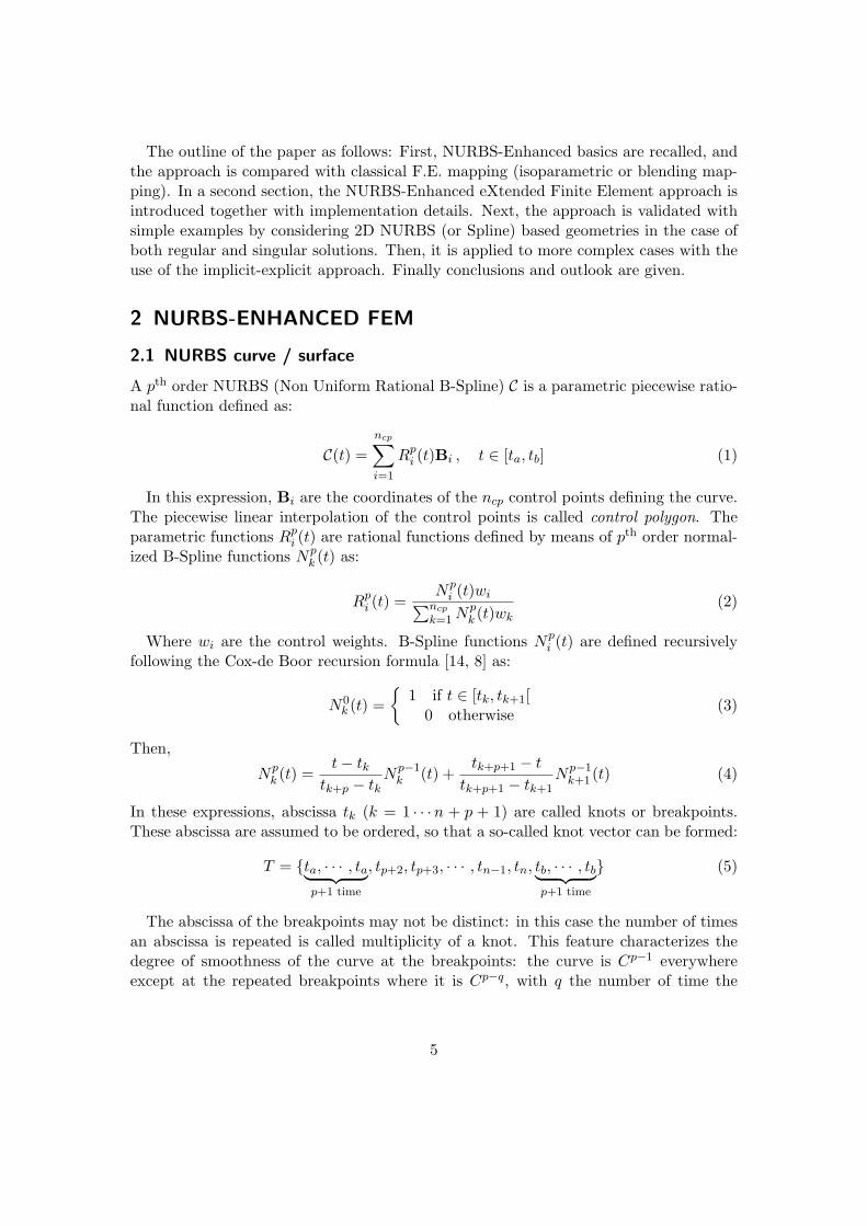
breakpoint is repeated. See for example Figure 1(a), where the following knot vectorwas considered for defining a quadratic Spline (which is a special instance of the NURBS,using constant weights wi = 1):

T = {0, 0, 0, 0.2, 0.4, 0.6,0.8,0.8, 1, 1, 1} (6)

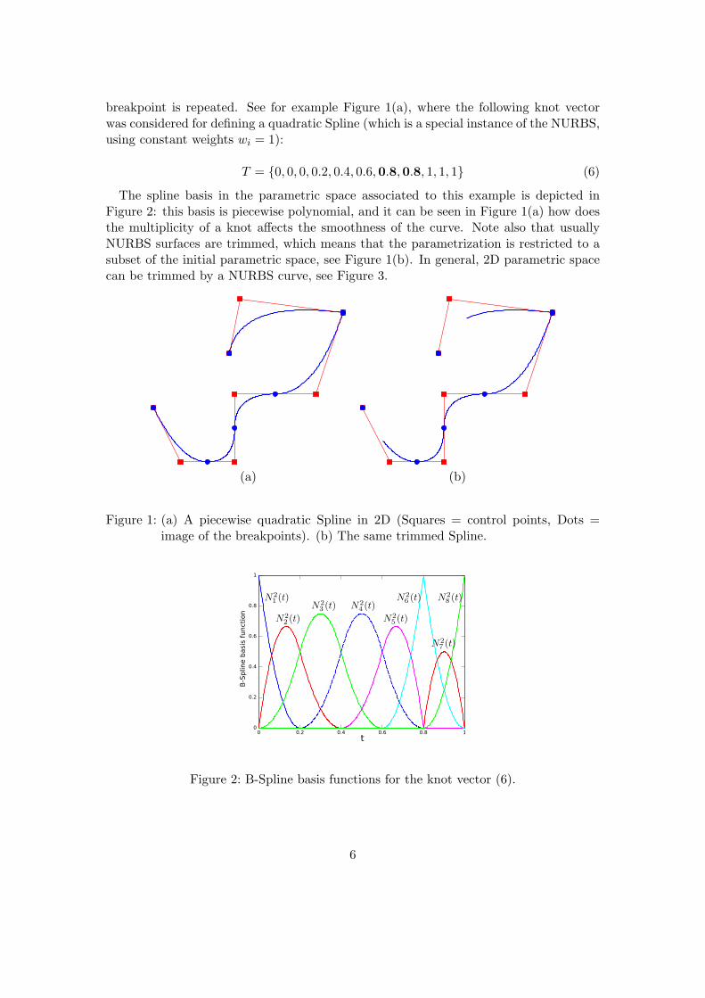
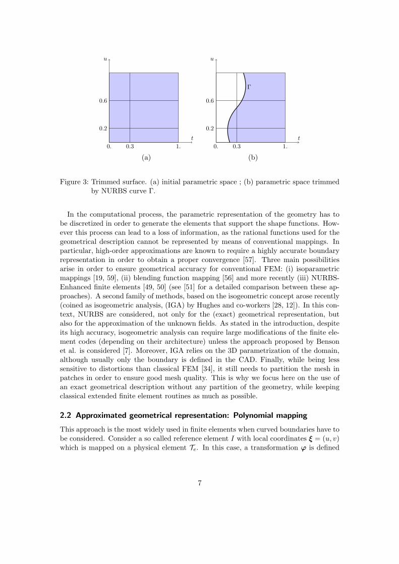
The spline basis in the parametric space associated to this example is depicted inFigure 2: this basis is piecewise polynomial, and it can be seen in Figure 1(a) how doesthe multiplicity of a knot affects the smoothness of the curve. Note also that usuallyNURBS surfaces are trimmed, which means that the parametrization is restricted to asubset of the initial parametric space, see Figure 1(b). In general, 2D parametric spacecan be trimmed by a NURBS curve, see Figure 3.

(a) (b)

Figure 1: (a) A piecewise quadratic Spline in 2D (Squares = control points, Dots =image of the breakpoints). (b) The same trimmed Spline.

0

0.2

0.4

0.6

0.8

1

0 0.2 0.4 0.6 0.8 1

B-Sp

line

basi

s fu

nctio

n

t

Figure 2: B-Spline basis functions for the knot vector (6).

6

0.30. 1.

0.2

0.6

u

t

Γ

0.30. 1.

0.2

0.6

u

t

(a) (b)

Figure 3: Trimmed surface. (a) initial parametric space ; (b) parametric space trimmedby NURBS curve Γ.

In the computational process, the parametric representation of the geometry has tobe discretized in order to generate the elements that support the shape functions. How-ever this process can lead to a loss of information, as the rational functions used for thegeometrical description cannot be represented by means of conventional mappings. Inparticular, high-order approximations are known to require a highly accurate boundaryrepresentation in order to obtain a proper convergence [57]. Three main possibilitiesarise in order to ensure geometrical accuracy for conventional FEM: (i) isoparametricmappings [19, 59], (ii) blending function mapping [56] and more recently (iii) NURBS-Enhanced finite elements [49, 50] (see [51] for a detailed comparison between these ap-proaches). A second family of methods, based on the isogeometric concept arose recently(coined as isogeometric analysis, (IGA) by Hughes and co-workers [28, 12]). In this con-text, NURBS are considered, not only for the (exact) geometrical representation, butalso for the approximation of the unknown fields. As stated in the introduction, despiteits high accuracy, isogeometric analysis can require large modifications of the finite ele-ment codes (depending on their architecture) unless the approach proposed by Bensonet al. is considered [7]. Moreover, IGA relies on the 3D parametrization of the domain,although usually only the boundary is defined in the CAD. Finally, while being lesssensitive to distortions than classical FEM [34], it still needs to partition the mesh inpatches in order to ensure good mesh quality. This is why we focus here on the use ofan exact geometrical description without any partition of the geometry, while keepingclassical extended finite element routines as much as possible.

2.2 Approximated geometrical representation: Polynomial mapping

This approach is the most widely used in finite elements when curved boundaries have tobe considered. Consider a so called reference element I with local coordinates ξ = (u, v)which is mapped on a physical element Te. In this case, a transformation ϕ is defined

7

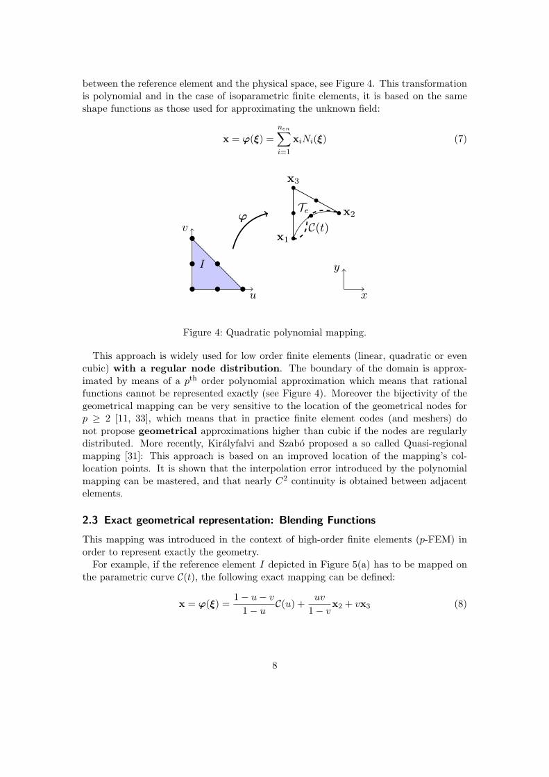
between the reference element and the physical space, see Figure 4. This transformationis polynomial and in the case of isoparametric finite elements, it is based on the sameshape functions as those used for approximating the unknown field:

x = ϕ(ξ) =

nen∑

i=1

xiNi(ξ) (7)

u

v

I

x

y

Teϕ

x1

x3

x2

C(t)

Figure 4: Quadratic polynomial mapping.

This approach is widely used for low order finite elements (linear, quadratic or evencubic) with a regular node distribution. The boundary of the domain is approx-imated by means of a pth order polynomial approximation which means that rationalfunctions cannot be represented exactly (see Figure 4). Moreover the bijectivity of thegeometrical mapping can be very sensitive to the location of the geometrical nodes forp ≥ 2 [11, 33], which means that in practice finite element codes (and meshers) donot propose geometrical approximations higher than cubic if the nodes are regularlydistributed. More recently, Kiralyfalvi and Szabo proposed a so called Quasi-regionalmapping [31]: This approach is based on an improved location of the mapping’s col-location points. It is shown that the interpolation error introduced by the polynomialmapping can be mastered, and that nearly C2 continuity is obtained between adjacentelements.

2.3 Exact geometrical representation: Blending Functions

This mapping was introduced in the context of high-order finite elements (p-FEM) inorder to represent exactly the geometry.For example, if the reference element I depicted in Figure 5(a) has to be mapped on

the parametric curve C(t), the following exact mapping can be defined:

x = ϕ(ξ) =1− u− v

1− uC(u) +

uv

1− vx2 + vx3 (8)

8

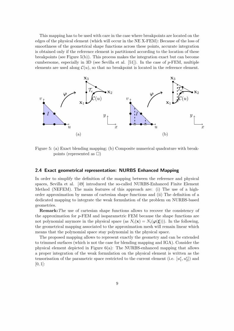
This mapping has to be used with care in the case where breakpoints are located on theedges of the physical element (which will occur in the NE X-FEM): Because of the loss ofsmoothness of the geometrical shape functions across these points, accurate integrationis obtained only if the reference element is partitioned according to the location of thesebreakpoints (see Figure 5(b)). This process makes the integration exact but can becomecumbersome, especially in 3D (see Sevilla et al. [51]). In the case of p-FEM, multipleelements are used along C(u), so that no breakpoint is located in the reference element.

u

v

I

x

y

Teϕ

x1

x3

x2

C(u)

u

v

I

� �

x

y

�

�

Teϕ

x1

x3

x2

C(u)

(a) (b)

Figure 5: (a) Exact blending mapping; (b) Composite numerical quadrature with break-points (represented as �)

2.4 Exact geometrical representation: NURBS Enhanced Mapping

In order to simplify the definition of the mapping between the reference and physicalspaces, Sevilla et al. [49] introduced the so-called NURBS-Enhanced Finite ElementMethod (NEFEM). The main features of this approach are: (i) The use of a high-order approximation by means of cartesian shape functions and (ii) The definition of adedicated mapping to integrate the weak formulation of the problem on NURBS-basedgeometries.Remark:The use of cartesian shape functions allows to recover the consistency of

the approximation for p-FEM and isoparametric FEM because the shape functions arenot polynomial anymore in the physical space (as Ni(x) = Ni(ϕ(ξ))). In the following,the geometrical mapping associated to the approximation mesh will remain linear whichmeans that the polynomial space stay polynomial in the physical space.The proposed mapping allows to represent exactly the geometry and can be extended

to trimmed surfaces (which is not the case for blending mapping and IGA). Consider thephysical element depicted in Figure 6(a): The NURBS-enhanced mapping that allowsa proper integration of the weak formulation on the physical element is written as thetensorisation of the parametric space restricted to the current element (i.e. [ue1, u

e2]) and

[0, 1]:

9

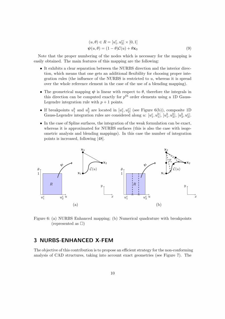
(u, θ) ∈ R = [ue1, ue2]× [0, 1]

ψ(u, θ) = (1− θ)C(u) + θx3 (9)

Note that the proper numbering of the nodes which is necessary for the mapping iseasily obtained. The main features of this mapping are the following:

• It exhibits a clear separation between the NURBS direction and the interior direc-tion, which means that one gets an additional flexibility for choosing proper inte-gration rules (the influence of the NURBS is restricted to u, whereas it is spreadover the whole reference element in the case of the use of a blending mapping).

• The geometrical mapping ψ is linear with respect to θ, therefore the integrals inthis direction can be computed exactly for pth order elements using a 1D Gauss-Legendre integration rule with p+ 1 points.

• If breakpoints ub1 and ub2 are located in [ue1, ue2] (see Figure 6(b)), composite 1D

Gauss-Legendre integration rules are considered along u: [ue1, ub1], [u

b1, u

b2], [u

b2, u

e2].

• In the case of Spline surfaces, the integration of the weak formulation can be exact,whereas it is approximated for NURBS surfaces (this is also the case with isoge-ometric analysis and blending mappings). In this case the number of integrationpoints is increased, following [48].

ue1

ue2

1

u

θ

x

y

ψ

x1

x3

x2

C(u)

R

ue1

ue2

1

u

θ

� �

x

y

Teψ

x1

x3

x2

�

�

C(u)

R

(a) (b)

Figure 6: (a) NURBS Enhanced mapping; (b) Numerical quadrature with breakpoints(represented as �)

3 NURBS-ENHANCED X-FEM

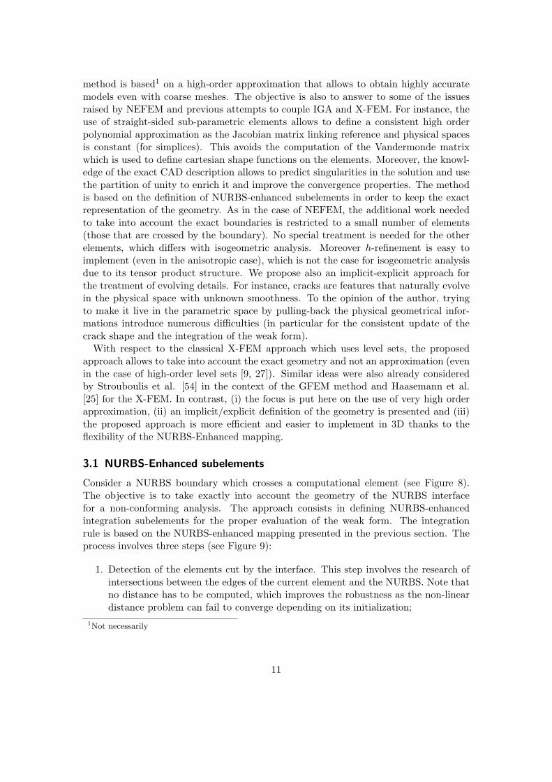
The objective of this contribution is to propose an efficient strategy for the non-conforminganalysis of CAD structures, taking into account exact geometries (see Figure 7). The

10

method is based1 on a high-order approximation that allows to obtain highly accuratemodels even with coarse meshes. The objective is also to answer to some of the issuesraised by NEFEM and previous attempts to couple IGA and X-FEM. For instance, theuse of straight-sided sub-parametric elements allows to define a consistent high orderpolynomial approximation as the Jacobian matrix linking reference and physical spacesis constant (for simplices). This avoids the computation of the Vandermonde matrixwhich is used to define cartesian shape functions on the elements. Moreover, the knowl-edge of the exact CAD description allows to predict singularities in the solution and usethe partition of unity to enrich it and improve the convergence properties. The methodis based on the definition of NURBS-enhanced subelements in order to keep the exactrepresentation of the geometry. As in the case of NEFEM, the additional work neededto take into account the exact boundaries is restricted to a small number of elements(those that are crossed by the boundary). No special treatment is needed for the otherelements, which differs with isogeometric analysis. Moreover h-refinement is easy toimplement (even in the anisotropic case), which is not the case for isogeometric analysisdue to its tensor product structure. We propose also an implicit-explicit approach forthe treatment of evolving details. For instance, cracks are features that naturally evolvein the physical space with unknown smoothness. To the opinion of the author, tryingto make it live in the parametric space by pulling-back the physical geometrical infor-mations introduce numerous difficulties (in particular for the consistent update of thecrack shape and the integration of the weak form).With respect to the classical X-FEM approach which uses level sets, the proposed

approach allows to take into account the exact geometry and not an approximation (evenin the case of high-order level sets [9, 27]). Similar ideas were also already consideredby Strouboulis et al. [54] in the context of the GFEM method and Haasemann et al.[25] for the X-FEM. In contrast, (i) the focus is put here on the use of very high orderapproximation, (ii) an implicit/explicit definition of the geometry is presented and (iii)the proposed approach is more efficient and easier to implement in 3D thanks to theflexibility of the NURBS-Enhanced mapping.

3.1 NURBS-Enhanced subelements

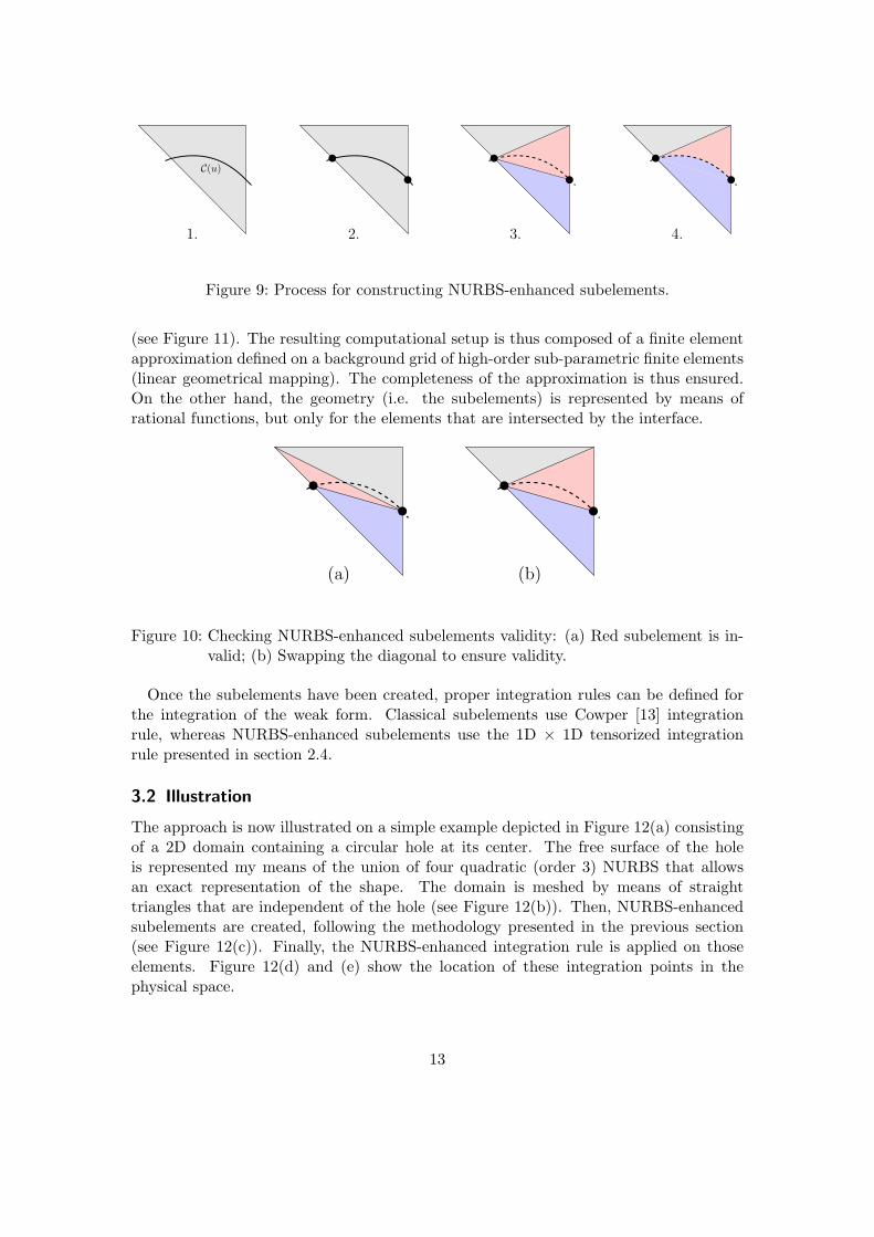
Consider a NURBS boundary which crosses a computational element (see Figure 8).The objective is to take exactly into account the geometry of the NURBS interfacefor a non-conforming analysis. The approach consists in defining NURBS-enhancedintegration subelements for the proper evaluation of the weak form. The integrationrule is based on the NURBS-enhanced mapping presented in the previous section. Theprocess involves three steps (see Figure 9):

1. Detection of the elements cut by the interface. This step involves the research ofintersections between the edges of the current element and the NURBS. Note thatno distance has to be computed, which improves the robustness as the non-lineardistance problem can fail to converge depending on its initialization;

1Not necessarily

11

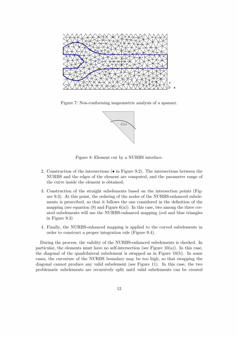
Figure 7: Non-conforming isogeometric analysis of a spanner.

C(u)

Figure 8: Element cut by a NURBS interface.

2. Construction of the intersections (• in Figure 9.2). The intersections between theNURBS and the edges of the element are computed, and the parameter range ofthe curve inside the element is obtained;

3. Construction of the straight subelements based on the intersection points (Fig-ure 9.3). At this point, the ordering of the nodes of the NURBS-enhanced subele-ments is prescribed, so that it follows the one considered in the definition of themapping (see equation (9) and Figure 6(a)). In this case, two among the three cre-ated subelements will use the NURBS-enhanced mapping (red and blue trianglesin Figure 9.3)

4. Finally, the NURBS-enhanced mapping is applied to the curved subelements inorder to construct a proper integration rule (Figure 9.4).

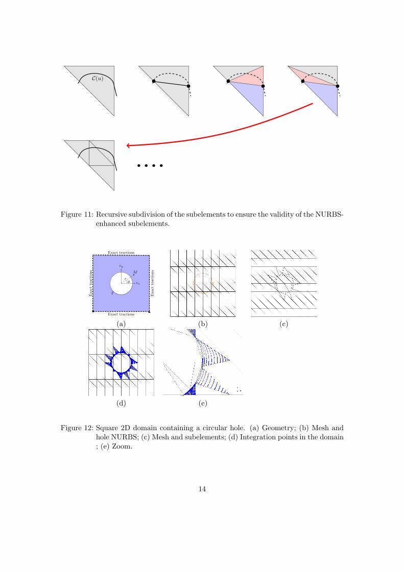
During the process, the validity of the NURBS-enhanced subelements is checked. Inparticular, the elements must have no self-intersection (see Figure 10(a)). In this case,the diagonal of the quadrilateral subelement is swapped as in Figure 10(b). In somecases, the curvature of the NURBS boundary may be too high, so that swapping thediagonal cannot produce any valid subelement (see Figure 11). In this case, the twoproblematic subelements are recursively split until valid subelements can be created

12

C(u)

1. 2. 3. 4.

Figure 9: Process for constructing NURBS-enhanced subelements.

(see Figure 11). The resulting computational setup is thus composed of a finite elementapproximation defined on a background grid of high-order sub-parametric finite elements(linear geometrical mapping). The completeness of the approximation is thus ensured.On the other hand, the geometry (i.e. the subelements) is represented by means ofrational functions, but only for the elements that are intersected by the interface.

(a) (b)

Figure 10: Checking NURBS-enhanced subelements validity: (a) Red subelement is in-valid; (b) Swapping the diagonal to ensure validity.

Once the subelements have been created, proper integration rules can be defined forthe integration of the weak form. Classical subelements use Cowper [13] integrationrule, whereas NURBS-enhanced subelements use the 1D × 1D tensorized integrationrule presented in section 2.4.

3.2 Illustration

The approach is now illustrated on a simple example depicted in Figure 12(a) consistingof a 2D domain containing a circular hole at its center. The free surface of the holeis represented my means of the union of four quadratic (order 3) NURBS that allowsan exact representation of the shape. The domain is meshed by means of straighttriangles that are independent of the hole (see Figure 12(b)). Then, NURBS-enhancedsubelements are created, following the methodology presented in the previous section(see Figure 12(c)). Finally, the NURBS-enhanced integration rule is applied on thoseelements. Figure 12(d) and (e) show the location of these integration points in thephysical space.

13

C(u)

Figure 11: Recursive subdivision of the subelements to ensure the validity of the NURBS-enhanced subelements.

Γ

ex

ey

M

θr

Exact tractions

Exact tractions

Exacttraction

s

Exacttraction

s

(a) (b) (c)

(d) (e)

Figure 12: Square 2D domain containing a circular hole. (a) Geometry; (b) Mesh andhole NURBS; (c) Mesh and subelements; (d) Integration points in the domain; (e) Zoom.

14

4 VERIFICATIONS

The method is now applied on structures containing boundaries defined by means ofNURBS and Splines. Focus is put on the convergence properties of the approximationin the case of both regular and singular solutions. All the problems assume a linearelastic material behaviour and the small strain assumption.

4.1 Plate with a hole

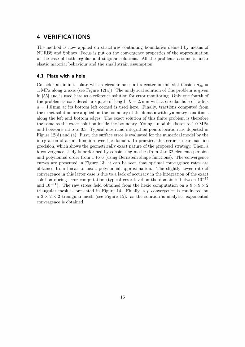
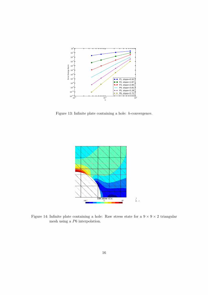
Consider an infinite plate with a circular hole in its center in uniaxial tension σ∞ =1.MPa along x axis (see Figure 12(a)). The analytical solution of this problem is givenin [55] and is used here as a reference solution for error monitoring. Only one fourth ofthe problem is considered: a square of length L = 2.mm with a circular hole of radiusa = 1.0mm at its bottom left corned is used here. Finally, tractions computed fromthe exact solution are applied on the boundary of the domain with symmetry conditionsalong the left and bottom edges. The exact solution of this finite problem is thereforethe same as the exact solution inside the boundary. Young’s modulus is set to 1.0 MPaand Poisson’s ratio to 0.3. Typical mesh and integration points location are depicted inFigure 12(d) and (e). First, the surface error is evaluated for the numerical model by theintegration of a unit function over the domain. In practice, this error is near machineprecision, which shows the geometrically exact nature of the proposed strategy. Then, ah-convergence study is performed by considering meshes from 2 to 32 elements per sideand polynomial order from 1 to 6 (using Bernstein shape functions). The convergencecurves are presented in Figure 13: it can be seen that optimal convergence rates areobtained from linear to hexic polynomial approximation. The slightly lower rate ofconvergence in this latter case is due to a lack of accuracy in the integration of the exactsolution during error computation (typical error level on the domain is between 10−15

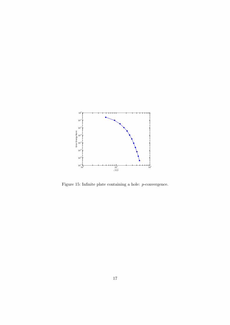
and 10−11). The raw stress field obtained from the hexic computation on a 9 × 9 × 2triangular mesh is presented in Figure 14. Finally, a p convergence is conducted ona 2 × 2 × 2 triangular mesh (see Figure 15): as the solution is analytic, exponentialconvergence is obtained.

15

10-2 10-1 100

h

10-11

10-10

10-9

10-8

10-7

10-6

10-5

10-4

10-3

10-2

10-1

100

Erro

r Ene

rgy

Norm

P1, slope=0.92P2, slope=1.87P3, slope=2.85P4, slope=3.81P5, slope=5.28P6, slope=5.72

Figure 13: Infinite plate containing a hole: h-convergence.

Figure 14: Infinite plate containing a hole: Raw stress state for a 9 × 9 × 2 triangularmesh using a P6 interpolation.

16

100 101 102√dofs

10-7

10-6

10-5

10-4

10-3

10-2

10-1

100

Erro

r Ene

rgy

Norm

Figure 15: Infinite plate containing a hole: p-convergence.

17

4.2 L-Shaped Panel

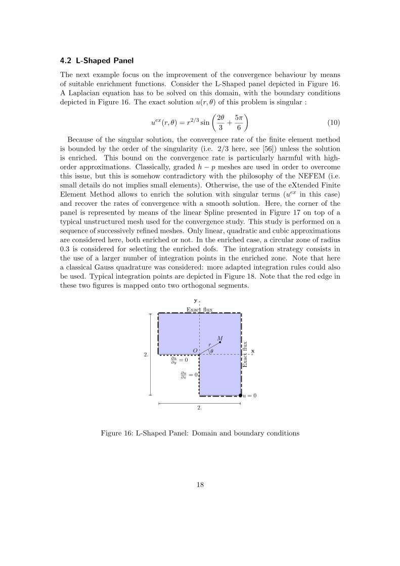
The next example focus on the improvement of the convergence behaviour by meansof suitable enrichment functions. Consider the L-Shaped panel depicted in Figure 16.A Laplacian equation has to be solved on this domain, with the boundary conditionsdepicted in Figure 16. The exact solution u(r, θ) of this problem is singular :

uex(r, θ) = r2/3 sin

(2θ

3+

5π

6

)

(10)

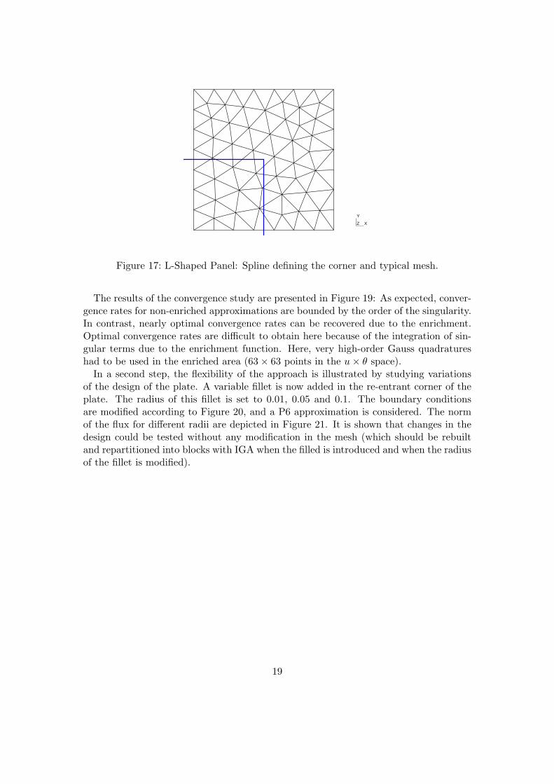
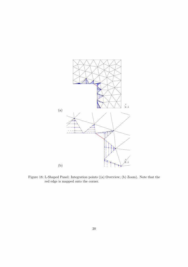
Because of the singular solution, the convergence rate of the finite element methodis bounded by the order of the singularity (i.e. 2/3 here, see [56]) unless the solutionis enriched. This bound on the convergence rate is particularly harmful with high-order approximations. Classically, graded h − p meshes are used in order to overcomethis issue, but this is somehow contradictory with the philosophy of the NEFEM (i.e.small details do not implies small elements). Otherwise, the use of the eXtended FiniteElement Method allows to enrich the solution with singular terms (uex in this case)and recover the rates of convergence with a smooth solution. Here, the corner of thepanel is represented by means of the linear Spline presented in Figure 17 on top of atypical unstructured mesh used for the convergence study. This study is performed on asequence of successively refined meshes. Only linear, quadratic and cubic approximationsare considered here, both enriched or not. In the enriched case, a circular zone of radius0.3 is considered for selecting the enriched dofs. The integration strategy consists inthe use of a larger number of integration points in the enriched zone. Note that herea classical Gauss quadrature was considered: more adapted integration rules could alsobe used. Typical integration points are depicted in Figure 18. Note that the red edge inthese two figures is mapped onto two orthogonal segments.

O x

y

Mrθ

∂u∂x

= 0

∂u∂y

= 0

Exact flux

Exactflux

u = 0

2.

2.

Figure 16: L-Shaped Panel: Domain and boundary conditions

18

X

Y

Z

Figure 17: L-Shaped Panel: Spline defining the corner and typical mesh.

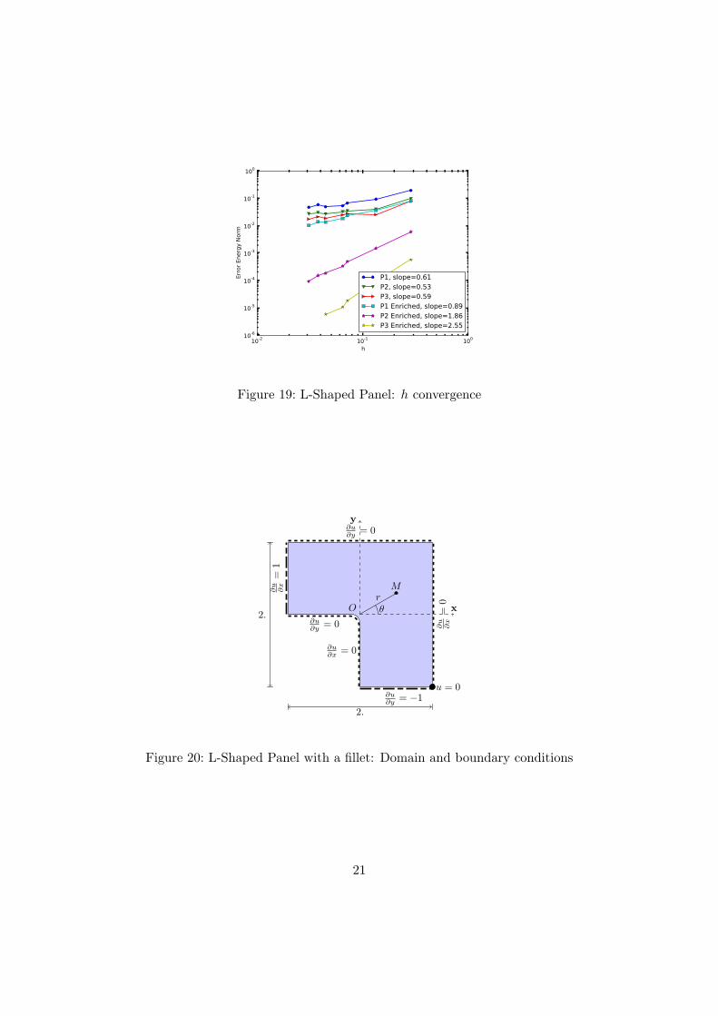
The results of the convergence study are presented in Figure 19: As expected, conver-gence rates for non-enriched approximations are bounded by the order of the singularity.In contrast, nearly optimal convergence rates can be recovered due to the enrichment.Optimal convergence rates are difficult to obtain here because of the integration of sin-gular terms due to the enrichment function. Here, very high-order Gauss quadratureshad to be used in the enriched area (63× 63 points in the u× θ space).

In a second step, the flexibility of the approach is illustrated by studying variationsof the design of the plate. A variable fillet is now added in the re-entrant corner of theplate. The radius of this fillet is set to 0.01, 0.05 and 0.1. The boundary conditionsare modified according to Figure 20, and a P6 approximation is considered. The normof the flux for different radii are depicted in Figure 21. It is shown that changes in thedesign could be tested without any modification in the mesh (which should be rebuiltand repartitioned into blocks with IGA when the filled is introduced and when the radiusof the fillet is modified).

19

(a)X

Y

Z

(b)X

Y

Z

Figure 18: L-Shaped Panel: Integration points ((a) Overview; (b) Zoom). Note that thered edge is mapped onto the corner.

20

10-2 10-1 100

h

10-6

10-5

10-4

10-3

10-2

10-1

100

Erro

r Ene

rgy

Norm

P1, slope=0.61P2, slope=0.53P3, slope=0.59P1 Enriched, slope=0.89P2 Enriched, slope=1.86P3 Enriched, slope=2.55

Figure 19: L-Shaped Panel: h convergence

O x

y

Mrθ

∂u∂x

= 0

∂u∂y

= 0

∂u∂y

= 0

∂u

∂x=

0

∂u∂y

= −1

∂u

∂x=

1

u = 0

2.

2.

Figure 20: L-Shaped Panel with a fillet: Domain and boundary conditions

21

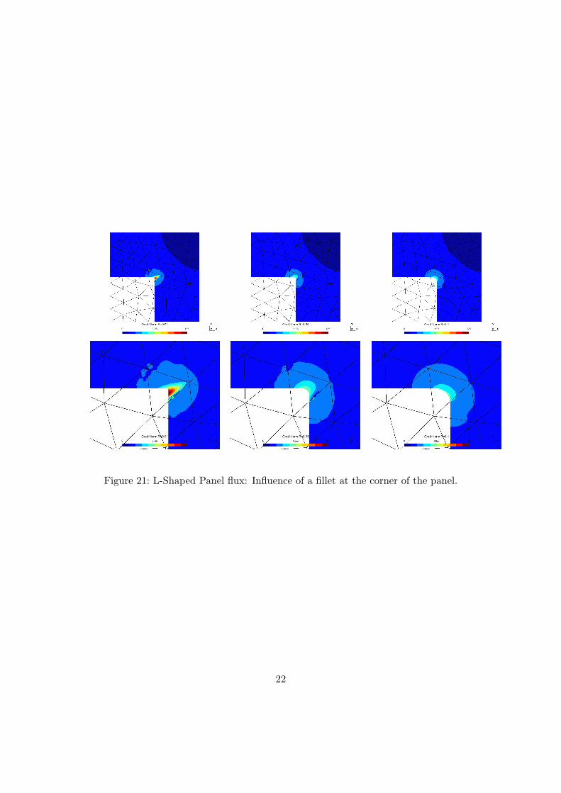
Figure 21: L-Shaped Panel flux: Influence of a fillet at the corner of the panel.

22

4.3 Material interfaces

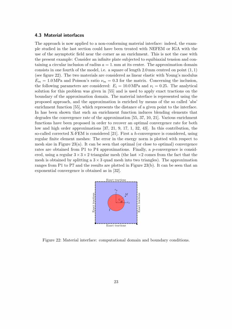
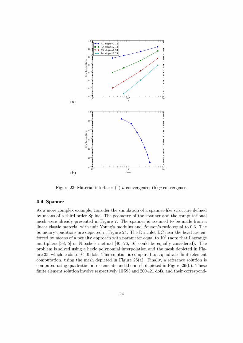
The approach is now applied to a non-conforming material interface: indeed, the exam-ple studied in the last section could have been treated with NEFEM or IGA with theuse of the asymptotic field near the corner as an enrichment. This is not the case withthe present example: Consider an infinite plate subjected to equibiaxial tension and con-taining a circular inclusion of radius a = 1.mm at its center. The approximation domainconsists in one fourth of the model, i.e. a square of length 2.0mm centred on point (1, 1)(see figure 22). The two materials are considered as linear elastic with Young’s modulusEm = 1.0MPa and Poisson’s ratio νm = 0.3 for the matrix. Concerning the inclusion,the following parameters are considered: Ei = 10.0MPa and νi = 0.25. The analyticalsolution for this problem was given in [55] and is used to apply exact tractions on theboundary of the approximation domain. The material interface is represented using theproposed approach, and the approximation is enriched by means of the so called ’abs’enrichment function [55], which represents the distance of a given point to the interface.In has been shown that such an enrichment function induces blending elements thatdegrades the convergence rate of the approximation [55, 37, 10, 21]. Various enrichmentfunctions have been proposed in order to recover an optimal convergence rate for bothlow and high order approximations [37, 21, 9, 17, 1, 32, 43]. In this contribution, theso-called corrected X-FEM is considered [21]. First a h-convergence is considered, usingregular finite element meshes: The error in the energy norm is plotted with respect tomesh size in Figure 23(a). It can be seen that optimal (or close to optimal) convergencerates are obtained from P1 to P4 approximations. Finally, a p-convergence is consid-ered, using a regular 3× 3× 2 triangular mesh (the last ×2 comes from the fact that themesh is obtained by splitting a 3× 3 quad mesh into two triangles). The approximationranges from P1 to P7 and the results are plotted in Figure 23(b). It can be seen that anexponential convergence is obtained as in [32].

Γ

ex

ey

M

θr

Exact tractions

Exact tractions

Exacttractions

Exacttractions

Figure 22: Material interface: computational domain and boundary conditions.

23

(a)10-2 10-1 100

h

10-7

10-6

10-5

10-4

10-3

10-2

10-1

100

Erro

r Ene

rgy

Norm

P1, slope=1.12P2, slope=2.14P3, slope=2.94P4, slope=3.77

(b)100 101 102√

dofs

10-6

10-5

10-4

10-3

10-2

10-1

100

Erro

r Ene

rgy

Norm

Figure 23: Material interface: (a) h-convergence; (b) p-convergence.

4.4 Spanner

As a more complex example, consider the simulation of a spanner-like structure definedby means of a third order Spline. The geometry of the spanner and the computationalmesh were already presented in Figure 7. The spanner is assumed to be made from alinear elastic material with unit Young’s modulus and Poisson’s ratio equal to 0.3. Theboundary conditions are depicted in Figure 24. The Dirichlet BC near the head are en-forced by means of a penalty approach with parameter equal to 106 (note that Lagrangemultipliers [38, 5] or Nitsche’s method [40, 26, 16] could be equally considered). Theproblem is solved using a hexic polynomial interpolation and the mesh depicted in Fig-ure 25, which leads to 9 410 dofs. This solution is compared to a quadratic finite elementcomputation, using the mesh depicted in Figure 26(a). Finally, a reference solution iscomputed using quadratic finite elements and the mesh depicted in Figure 26(b). Thesefinite element solution involve respectively 10 593 and 200 421 dofs, and their correspond-

24

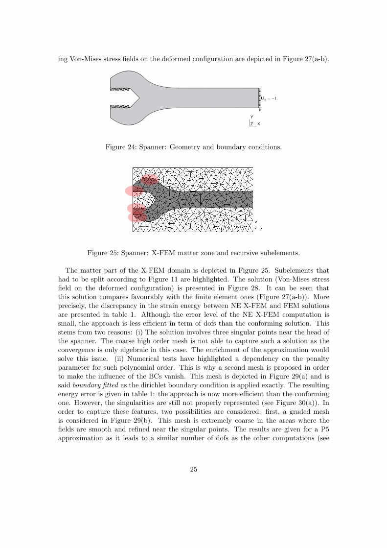
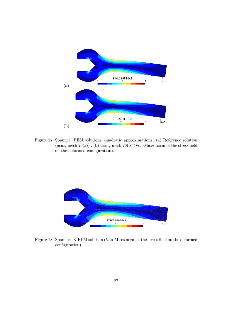
ing Von-Mises stress fields on the deformed configuration are depicted in Figure 27(a-b).

X

Y

Z

Figure 24: Spanner: Geometry and boundary conditions.

Figure 25: Spanner: X-FEM matter zone and recursive subelements.

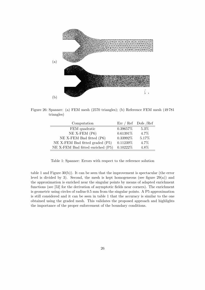
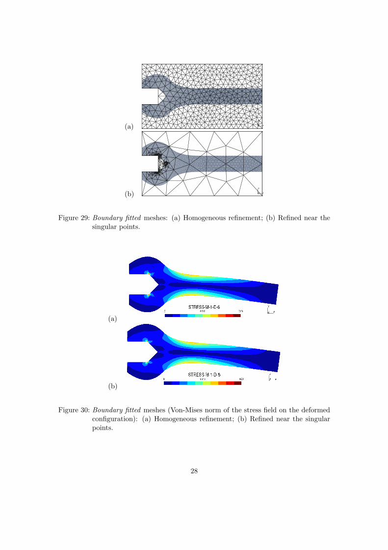
The matter part of the X-FEM domain is depicted in Figure 25. Subelements thathad to be split according to Figure 11 are highlighted. The solution (Von-Mises stressfield on the deformed configuration) is presented in Figure 28. It can be seen thatthis solution compares favourably with the finite element ones (Figure 27(a-b)). Moreprecisely, the discrepancy in the strain energy between NE X-FEM and FEM solutionsare presented in table 1. Although the error level of the NE X-FEM computation issmall, the approach is less efficient in term of dofs than the conforming solution. Thisstems from two reasons: (i) The solution involves three singular points near the head ofthe spanner. The coarse high order mesh is not able to capture such a solution as theconvergence is only algebraic in this case. The enrichment of the approximation wouldsolve this issue. (ii) Numerical tests have highlighted a dependency on the penaltyparameter for such polynomial order. This is why a second mesh is proposed in orderto make the influence of the BCs vanish. This mesh is depicted in Figure 29(a) and issaid boundary fitted as the dirichlet boundary condition is applied exactly. The resultingenergy error is given in table 1: the approach is now more efficient than the conformingone. However, the singularities are still not properly represented (see Figure 30(a)). Inorder to capture these features, two possibilities are considered: first, a graded meshis considered in Figure 29(b). This mesh is extremely coarse in the areas where thefields are smooth and refined near the singular points. The results are given for a P5approximation as it leads to a similar number of dofs as the other computations (see

25

(a)

(b)

Figure 26: Spanner: (a) FEM mesh (2570 triangles); (b) Reference FEM mesh (49 781triangles)

Computation Err / Ref Dofs /Ref

FEM quadratic 0.39657% 5.3%NE X-FEM (P6) 0.61391% 4.7%

NE X-FEM Bnd fitted (P6) 0.33992% 5.17%NE X-FEM Bnd fitted graded (P5) 0.11239% 4.7%NE X-FEM Bnd fitted enriched (P5) 0.10222% 4.8%

Table 1: Spanner: Errors with respect to the reference solution

table 1 and Figure 30(b)). It can be seen that the improvement is spectacular (the errorlevel is divided by 3). Second, the mesh is kept homogeneous (see figure 29(a)) andthe approximation is enriched near the singular points by means of adapted enrichmentfunctions (see [52] for the derivation of asymptotic fields near corners). The enrichmentis geometric using circles of radius 0.5 mm from the singular points. A P5 approximationis still considered and it can be seen in table 1 that the accuracy is similar to the oneobtained using the graded mesh. This validates the proposed approach and highlightsthe importance of the proper enforcement of the boundary conditions.

26

(a)

(b)

Figure 27: Spanner: FEM solutions, quadratic approximations: (a) Reference solution(using mesh 26(a)) ; (b) Using mesh 26(b) (Von-Mises norm of the stress fieldon the deformed configuration).

Figure 28: Spanner: X-FEM solution (Von-Mises norm of the stress field on the deformedconfiguration).

27

(a) X

Y

Z X

Y

Z

(b) X

Y

Z X

Y

Z

Figure 29: Boundary fitted meshes: (a) Homogeneous refinement; (b) Refined near thesingular points.

(a)

(b)

Figure 30: Boundary fitted meshes (Von-Mises norm of the stress field on the deformedconfiguration): (a) Homogeneous refinement; (b) Refined near the singularpoints.

28

4.5 Coupling NE X-FEM and Sub-Grid level sets

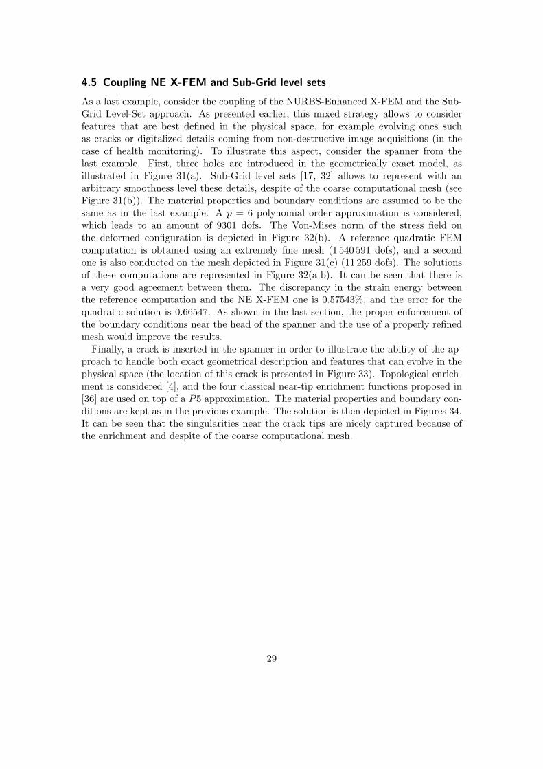
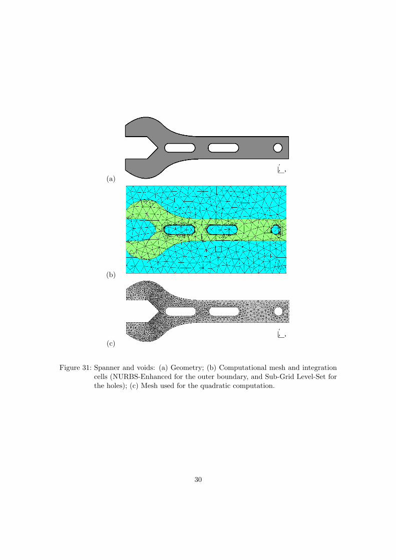
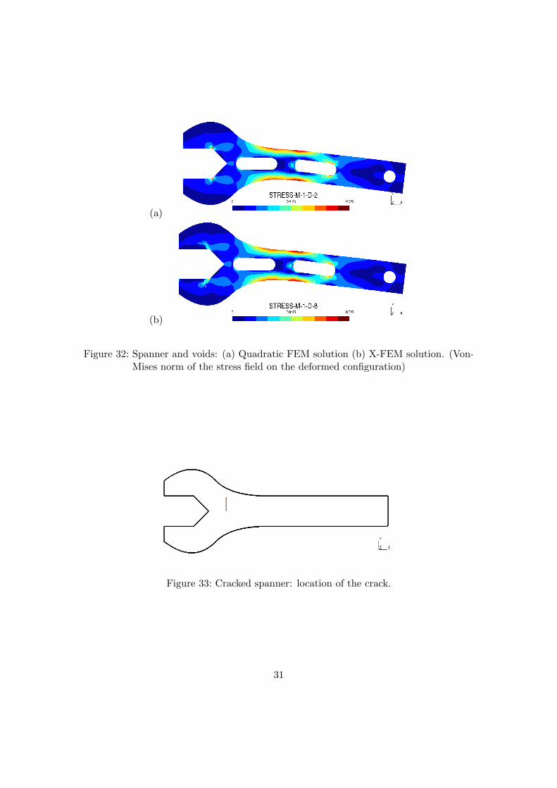
As a last example, consider the coupling of the NURBS-Enhanced X-FEM and the Sub-Grid Level-Set approach. As presented earlier, this mixed strategy allows to considerfeatures that are best defined in the physical space, for example evolving ones suchas cracks or digitalized details coming from non-destructive image acquisitions (in thecase of health monitoring). To illustrate this aspect, consider the spanner from thelast example. First, three holes are introduced in the geometrically exact model, asillustrated in Figure 31(a). Sub-Grid level sets [17, 32] allows to represent with anarbitrary smoothness level these details, despite of the coarse computational mesh (seeFigure 31(b)). The material properties and boundary conditions are assumed to be thesame as in the last example. A p = 6 polynomial order approximation is considered,which leads to an amount of 9301 dofs. The Von-Mises norm of the stress field onthe deformed configuration is depicted in Figure 32(b). A reference quadratic FEMcomputation is obtained using an extremely fine mesh (1 540 591 dofs), and a secondone is also conducted on the mesh depicted in Figure 31(c) (11 259 dofs). The solutionsof these computations are represented in Figure 32(a-b). It can be seen that there isa very good agreement between them. The discrepancy in the strain energy betweenthe reference computation and the NE X-FEM one is 0.57543%, and the error for thequadratic solution is 0.66547. As shown in the last section, the proper enforcement ofthe boundary conditions near the head of the spanner and the use of a properly refinedmesh would improve the results.Finally, a crack is inserted in the spanner in order to illustrate the ability of the ap-

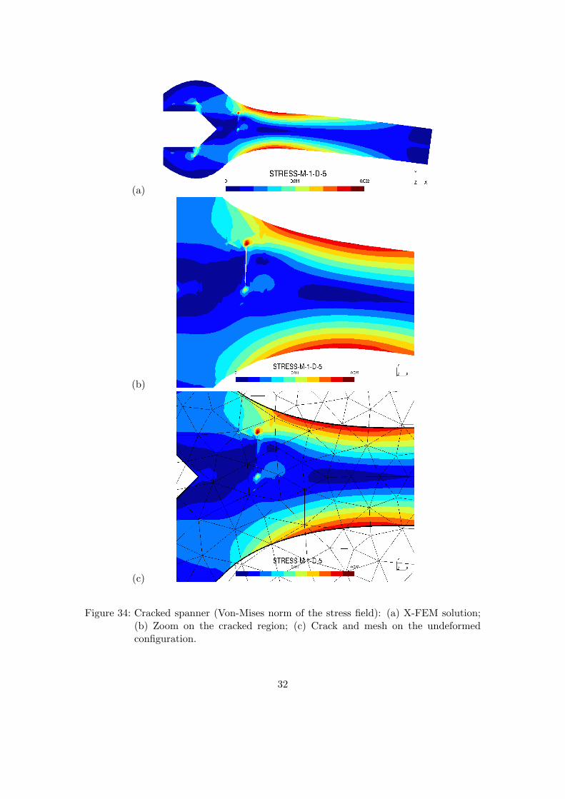
proach to handle both exact geometrical description and features that can evolve in thephysical space (the location of this crack is presented in Figure 33). Topological enrich-ment is considered [4], and the four classical near-tip enrichment functions proposed in[36] are used on top of a P5 approximation. The material properties and boundary con-ditions are kept as in the previous example. The solution is then depicted in Figures 34.It can be seen that the singularities near the crack tips are nicely captured because ofthe enrichment and despite of the coarse computational mesh.

29

(a)

(b)

(c)

Figure 31: Spanner and voids: (a) Geometry; (b) Computational mesh and integrationcells (NURBS-Enhanced for the outer boundary, and Sub-Grid Level-Set forthe holes); (c) Mesh used for the quadratic computation.

30

(a)

(b)

Figure 32: Spanner and voids: (a) Quadratic FEM solution (b) X-FEM solution. (Von-Mises norm of the stress field on the deformed configuration)

Figure 33: Cracked spanner: location of the crack.

31

(a)

(b)

(c)

Figure 34: Cracked spanner (Von-Mises norm of the stress field): (a) X-FEM solution;(b) Zoom on the cracked region; (c) Crack and mesh on the undeformedconfiguration.

32

5 CONCLUSION

An eXtended Finite Element approach was proposed for 2D unfitted geometrically ex-act analysis. This approach relies on two main ingredients: (i) the use of the exactboundaries by means of NURBS and Nurbs-Enhanced subelements and (ii) the use ofa partition of unity approach for enriching the non-conforming solution. With respectto isogeometric analysis, the proposed approach simplifies greatly the mesh refinementprocess. In addition, only the surface parametrization of the domain is necessary, whichis the only information a CAD modeller is working on. Finally, only a small part of theX-FEM code has to be modified. The NURBS-enhanced mapping is also more versa-tile than the blending function mapping proposed in [54] in the case of breakpoints ortrimmed NURBS inside an element (see [51, 50]), especially in 3D. It was demonstratedthat the use of a straight sided background mesh allows to define a consistent high-orderapproximation without the need of cartesian-based shape functions. Optimal conver-gence rates could be obtained. In addition, the knowledge of the parametrization of thesurface allows to predict automatically the location of singular points in the solution, andenrich the approximation accordingly. It was also proposed to use an implicit/explicitrepresentation of the geometry: explicit for the general geometry of the structure andimplicit for evolving features such as cracks. Great flexibility is added thanks to thismixed strategy. Work will now focus on the extension to the 3D case: the extension ofthe NURBS-enhanced mapping was already demonstrated in [50], so that this extensionwould depend on the ease of implementation in this more complex context. In the casewhere the regularity of the solution is of interest, arbitrary smooth approximation canalso be considered if a structured mesh and Spline-based shape functions are used. Inthis case, it is not necessary to extend the NURBS-enhanced mapping to quadranglesand hexaedra as proposed in [49]: The quadrangles (resp. hexaedra) can be split intotwo triangles (resp. six tetraedra) for the integration before applying the proposed ap-proach on this simplex mesh. Finally, note that the approach can be directly applied in3D for thin-walled structures, following the approach proposed by Rank et al. [42] withthe Finite Cell method.

Acknowledgement:The support of the ERC Advanced Grant XLS no 291102 is gratefully acknowledged

33

6 REFERENCES

References

[1] Babuska I, Banerjee U (2012) Stable Generalized Finite Element Method (SGFEM).Computer Methods in Applied Mechanics and Engineering 201-204:91–111, DOI10.1016/j.cma.2011.09.012, URL http://dx.doi.org/10.1016/j.cma.2011.09.012

[2] Bazilevs Y, Bajaj C, Calo V, Hughes T (2010) Special issue on com-putational geometry and analysis. Computer Methods in Applied Mechan-ics and Engineering 199(5–8):223–, DOI 10.1016/j.cma.2009.10.006, URLhttp://www.sciencedirect.com/science/article/pii/S0045782509003429

[3] Bazilevs Y, Calo V, Cottrell J, Evans J, Hughes T, Lipton S, Scott M, SederbergT (2010) Isogeometric analysis using T-splines. Computer Methods in Applied Me-chanics and Engineering 199(5–8):229–263, DOI 10.1016/j.cma.2009.02.036, URLhttp://www.sciencedirect.com/science/article/pii/S0045782509000875

[4] Bechet E, Minnebo H, Moes N, Burgardt B (2005) Improved implementation androbustness study of the X-FEM for stress analysis around cracks. InternationalJournal for Numerical Methods in Engineering 64(8):1033–1056

[5] Bechet E, Moes N, Wohlmuth B (2009) A stable lagrange multiplier space forthe stiff interface conditions within the extended finite element method. Inter-national Journal for Numerical Methods in Engineering 78(8):931–954, DOI10.1002/nme.2515

[6] Belytschko T, Parimi C, Moes N, Usui S, Sukumar N (2003) Structured extendedfinite element methods of solids defined by implicit surfaces. International Journalfor Numerical Methods in Engineering 56:609–635

[7] Benson DJ, Bazilevs Y, De Luycker E, Hsu MC, Scott M, Hughes TJR, Be-lytschko T (2010) A generalized finite element formulation for arbitrary ba-sis functions: From isogeometric analysis to XFEM. International Journal forNumerical Methods in Engineering 83(6):765–785, DOI 10.1002/nme.2864, URLhttp://dx.doi.org/10.1002/nme.2864

[8] Boor CD (1972) On calculation with B-splines. Journal of Approximation Theory6:50–62

[9] Cheng KW, Fries T (2009) Higher-order XFEM for curved strong and weak discon-tinuities. International Journal for Numerical Methods in Engineering 82:564–590,DOI 10.1002/nme.2768, URL http://doi.wiley.com/10.1002/nme.2768

[10] Chessa J, Wang H, Belytschko T (2003) On the construction of blending elements forlocal partition of unity enriched finite elements. International Journal for NumericalMethods in Engineering 57:1015–1038

34

[11] Ciarlet P, Raviart PA (1972) Interpolation theory over curved elements, withapplications to finite element methods. Computer Methods in Applied Me-chanics and Engineering 1(2):217–249, DOI 10.1016/0045-7825(72)90006-0, URLhttp://www.sciencedirect.com/science/article/pii/0045782572900060

[12] Cottrell J, Hughes TJ, Bazilevs Y (2009) Isogeometric Analysis: Toward Integrationof CAD and FE. John Wiley & Sons

[13] Cowper G (1973) Gaussian Quadrature Formulas for Triangles. International Jour-nal for Numerical Methods in Engineering 7:405–408

[14] Cox M (1971) The numerical evaluation of B-splines. Tech. Rep. DNAC 4, NationalPhysical Laboratory

[15] De Luycker E, Benson DJ, Belytschko T, Bazilevs Y, Hsu MC (2011) X-FEMin isogeometric analysis for linear fracture mechanics. International Journal forNumerical Methods in Engineering 87(6):541–565, DOI 10.1002/nme.3121, URLhttp://dx.doi.org/10.1002/nme.3121

[16] Dolbow J, Harari I (2009) An efficient finite element method for embedded interfaceproblems. International Journal for Numerical Methods in Engineering 78(2):229–252, DOI 10.1002/nme.2486, URL http://dx.doi.org/10.1002/nme.2486

[17] Dreau K, Chevaugeon N, Moes N (2010) Studied X-FEM enrichment to handlematerial interfaces with higher order finite element. Computer Methods in AppliedMechanics and Engineering 199(29-32):1922–1936, DOI 10.1016/j.cma.2010.01.021,URL http://linkinghub.elsevier.com/retrieve/pii/S0045782510000563

[18] Duster A, Parvizian J, Yang Z, Rank E (2008) The finite cell method for three-dimensional problems of solid mechanics. Computer Methods in Applied Mechan-ics and Engineering 197(45-48):3768–3782, DOI 10.1016/j.cma.2008.02.036, URLhttp://linkinghub.elsevier.com/retrieve/pii/S0045782508001163

[19] Ergatoudis I, Irons B, Zienkiewicz O (1968) Curved, isoparametric, “quadri-lateral” elements for finite element analysis. International Journal ofSolids and Structures 4(1):31–42, DOI 10.1016/0020-7683(68)90031-0, URLhttp://www.sciencedirect.com/science/article/pii/0020768368900310

[20] Forsey DR, Bartels RH (1988) Hierarchical B-spline refinement. SIG-GRAPH Comput Graph 22(4):205–212, DOI 10.1145/378456.378512, URLhttp://doi.acm.org.gate6.inist.fr/10.1145/378456.378512

[21] Fries T (2008) A corrected XFEM approximation without problems in blendingelements. International Journal for Numerical Methods in Engineering 75(5):503–532, DOI 10.1002/nme.2259, URL http://dx.doi.org/10.1002/nme.2259

35

[22] Fries TP, Belytschko T (2010) The extended/generalized finite element method:An overview of the method and its applications. International Journal for Nu-merical Methods in Engineering 84(3):253–304, DOI 10.1002/nme.2914, URLhttp://dx.doi.org/10.1002/nme.2914

[23] Ghorashi SS, Valizadeh N, Mohammadi S (2012) Extended isogeometric analy-sis for simulation of stationary and propagating cracks. International Journal forNumerical Methods in Engineering 89(9):1069–1101, DOI 10.1002/nme.3277, URLhttp://dx.doi.org/10.1002/nme.3277

[24] Gomez H, Calo VM, Bazilevs Y, Hughes TJ (2008) Isogeometric analysis ofthe Cahn–Hilliard phase-field model. Computer Methods in Applied Mechan-ics and Engineering 197(49–50):4333–4352, DOI 10.1016/j.cma.2008.05.003, URLhttp://www.sciencedirect.com/science/article/pii/S0045782508001953

[25] Haasemann G, Kastner M, Pruger S, Ulbricht V (2011) Development of a quadraticfinite element formulation based on the XFEM and NURBS. International Journalfor Numerical Methods in Engineering 86(4-5):598–617, DOI 10.1002/nme.3120,URL http://dx.doi.org/10.1002/nme.3120

[26] Hansbo A, Hansbo P (2004) A finite element method for the simulation of strongand weak discontinuities in solid mechanics. Computer Methods in AppliedMechanics and Engineering 193(33-35):3523–3540, DOI 10.1016/j.cma.2003.12.041,URL http://www.sciencedirect.com/science/article/B6V29-4BRSGX0-4/2/0a5f9d036b9ef16b2a0e571b247ff04d

[27] Huerta A, Casoni E, Sala-Lardies E, Fernandez-Mendez S, Peraire J (2010) Model-ing discontinuities with high-order elements. In: ECCM 2010 - Paris

[28] Hughes T, Cottrell J, Bazilevs Y (2005) Isogeometric analysis: CAD, finite elements,NURBS, exact geometry and mesh refinement. Computer Methods in Applied Me-chanics and Engineering 194(39–41):4135–4195, DOI 10.1016/j.cma.2004.10.008,URL http://www.sciencedirect.com/science/article/pii/S0045782504005171

[29] Kim HJ, Seo YD, Youn SK (2009) Isogeometric analysis for trimmedCAD surfaces. Computer Methods in Applied Mechanics and Engi-neering 198(37–40):2982–2995, DOI 10.1016/j.cma.2009.05.004, URLhttp://www.sciencedirect.com/science/article/pii/S0045782509001856

[30] Kim HJ, Seo YD, Youn SK (2010) Isogeometric analysis with trimming techniquefor problems of arbitrary complex topology. Computer Methods in Applied Mechan-ics and Engineering 199(45–48):2796–2812, DOI 10.1016/j.cma.2010.04.015, URLhttp://www.sciencedirect.com/science/article/pii/S0045782510001325

[31] Kiralyfalvi G, Szabo B (1997) Quasi-regional mapping for the p-version of the finite element method. Finite Elements in Analysisand Design 27(1):85–97, DOI 10.1016/S0168-874X(97)00006-1, URLhttp://linkinghub.elsevier.com/retrieve/pii/S0168874X97000061

36

[32] Legrain G, Chevaugeon N, Dreau K (2012) High order X-FEM andlevelsets for complex microstructures: Uncoupling geometry and ap-proximation. Computer Methods in Applied Mechanics and Engi-neering 241–244(0):172–189, DOI 10.1016/j.cma.2012.06.001, URLhttp://www.sciencedirect.com/science/article/pii/S0045782512001880

[33] Lenoir M (1986) Optimal Isoparametric Finite Elements and Er-ror Estimates for Domains Involving Curved Boundaries. SIAM Jour-nal on Numerical Analysis 23(3):562–580, DOI 10.1137/0723036, URLhttp://link.aip.org/link/?SNA/23/562/1

[34] Lipton S, Evans J, Bazilevs Y, Elguedj T, Hughes T (2010) Ro-bustness of isogeometric structural discretizations under severemesh distortion. Computer Methods in Applied Mechanics and En-gineering 199(5–8):357–373, DOI 10.1016/j.cma.2009.01.022, URLhttp://www.sciencedirect.com/science/article/pii/S0045782509000346

[35] Melenk J, Babuska I (1996) The partition of unity finite element method : Basictheory and applications. Comp Meth in Applied Mech and Engrg 139:289–314

[36] Moes N, Dolbow J, Belytschko T (1999) A finite element method for crack growthwithout remeshing. International Journal for Numerical Methods in Engineering46:131–150

[37] Moes N, Cloirec M, Cartraud P, Remacle JF (2003) A computational approach tohandle complex microstructure geometries. Comp Meth in Applied Mech and Engrg192:3163–3177, URL http://dx.doi.org/doi:10.1016/S0045-7825(03)00346-3

[38] Moes N, Bechet E, Tourbier M (2006) Imposing Dirichlet boundary conditions inthe extended finite element method. International Journal for Numerical Methodsin Engineering 67(12):1641–1669

[39] Moumnassi M, Belouettar S, Bechet E, Bordas SP, Quoirin D, Potier-Ferry M(2011) Finite element analysis on implicitly defined domains: An accurate rep-resentation based on arbitrary parametric surfaces. Computer Methods in AppliedMechanics and Engineering 200(5-8):774–796, DOI 10.1016/j.cma.2010.10.002, URLhttp://www.sciencedirect.com/science/article/pii/S004578251000280X

[40] Nitsche J (1971) Uber ein Variationprinzip zur losung von Dirichlet-Problem beiVerwendung von Teilraumen, die keinen Randbedingungen unterworfen sind. AbhMath Sem Univ Hamburg 36:9–15

[41] Parvizian J, Duster A, Rank E (2007) Finite cell method - h andp extension for embedded domain problems in solid mechanics. Com-putational Mechanics 41(1):121–133, DOI 10.1007/s00466-007-0173-y, URLhttp://www.springerlink.com/index/10.1007/s00466-007-0173-y

37

[42] Rank E, Ruess M, Kollmannsberger S, Schillinger D, Duster A(2012) Geometric modeling, isogeometric analysis and the finitecell method. Computer Methods in Applied Mechanics and En-gineering 249-252:104–115, DOI 10.1016/j.cma.2012.05.022, URLhttp://linkinghub.elsevier.com/retrieve/pii/S0045782512001855

[43] Sala-Lardies E, Huerta A (2012) Optimally Convergent High-Order X-FEM forProblems with Voids and Inclusions. In: Eccomas 2012

[44] Schillinger D, Rank E (2011) An unfitted hp-adaptive finite elementmethod based on hierarchical B-splines for interface problems of com-plex geometry. Computer Methods in Applied Mechanics and Engi-neering 200(47-48):3358–3380, DOI 10.1016/j.cma.2011.08.002, URLhttp://www.sciencedirect.com/science/article/pii/S004578251100257X

[45] Schillinger D, Duster A, Rank E (2011) The hp-d-adaptive finite cell methodfor geometrically nonlinear problems of solid mechanics. International Journal forNumerical Methods in Engineering pp n/a–n/a, DOI 10.1002/nme.3289, URLhttp://dx.doi.org/10.1002/nme.3289

[46] Schillinger D, Dede L, Scott MA, Evans JA, Borden MJ, Rank E,Hughes TJ (2012) An isogeometric design-through-analysis methodologybased on adaptive hierarchical refinement of NURBS, immersed bound-ary methods, and T-spline CAD surfaces. Computer Methods in Ap-plied Mechanics and Engineering (0):–, DOI 10.1016/j.cma.2012.03.017, URLhttp://www.sciencedirect.com/science/article/pii/S004578251200093X

[47] Sederberg TW, Zheng J, Bakenov A, Nasri A (2003) T-splines and T-NURCCs. ACM Trans Graph 22(3):477–484, DOI 10.1145/882262.882295, URLhttp://doi.acm.org.gate6.inist.fr/10.1145/882262.882295

[48] Sevilla R, Fernandez-Mendez S (2011) Numerical integration over 2D NURBS-shaped domains with applications to NURBS-enhanced FEM. Finite Elementsin Analysis and Design 47(10):1209–1220, DOI 10.1016/j.finel.2011.05.011, URLhttp://www.sciencedirect.com/science/article/pii/S0168874X1100117X

[49] Sevilla R, Fernandez-Mendez S, Huerta A (2008) NURBS-enhanced finite elementmethod (NEFEM). International Journal for Numerical Methods in Engineering76(1):56–83, DOI 10.1002/nme.2311, URL http://dx.doi.org/10.1002/nme.2311

[50] Sevilla R, Fernandez-Mendez S, Huerta A (2011) 3D NURBS-enhancedfinite element method (NEFEM). International Journal for NumericalMethods in Engineering 88(2):103–125, DOI 10.1002/nme.3164, URLhttp://dx.doi.org/10.1002/nme.3164

[51] Sevilla R, Fernandez-Mendez S, Huerta A (2011) Comparison of high-order curvedfinite elements. International Journal for Numerical Methods in Engineering87(8):719–734, DOI 10.1002/nme.3129, URL http://dx.doi.org/10.1002/nme.3129

38

[52] Seweryn A, Molski K (1996) Elastic stress singularities and corresponding gen-eralized stress intensity factors for angular corners under various boundary con-ditions. Engineering {F}racture {M}echanics 55(4):529–556, DOI 10.1016/S0013-7944(96)00035-5, URL http://dx.doi.org/10.1016/S0013-7944(96)00035-5

[53] Strouboulis T, Babuska I, Copps K (2000) The design and analysis of the generalizedfinite element method. Computer Methods in Applied Mechanics and Engineering181:43–69

[54] Strouboulis T, Copps K, Babuska I (2001) The generalized finite el-ement method. Computer Methods in Applied Mechanics and Engi-neering 190(32–33):4081–4193, DOI 10.1016/S0045-7825(01)00188-8, URLhttp://www.sciencedirect.com/science/article/pii/S0045782501001888

[55] Sukumar N, Chopp DL, Moes N, Belytschko T (2001) Modeling Holes and Inclusionsby Level Sets in the Extended Finite Element Method. Comp Meth in Applied Mechand Engrg 190:6183–6200, URL http://dx.doi.org/10.1016/S0045-7825(01)00215-8

[56] Szabo B, Babuska I (1991) Finite Element Analysis. John Wiley & Sons, New York

[57] Szabo B, Duster A, Rank E (2004) Encyclopedia of computational mechanics, JohnWiley, chap The p-version of the Finite Element Method, pp 120–140

[58] Yazid A, Abdelkader N, Abdelmadjid H (2009) A state-of-the-art re-view of the X-FEM for computational fracture mechanics. Applied Math-ematical Modelling 33(12):4269–4282, DOI 10.1016/j.apm.2009.02.010, URLhttp://www.sciencedirect.com/science/article/pii/S0307904X09000560

[59] Zienkiewicz OC, Taylor R (1991) The Finite Element Method, Vol. 1, 2, 3. McGraw-Hill, London

39