Embed Size (px)
Citation preview

Statistical Models for NetworksDifficulties of fitting the ERGM
Favored Approach: Approximate MLE via MCMC
Exponential Random Graph Models forNetwork Data
David Hunter
Department of StatisticsPenn State University
Student Organized Seminar, March 17, 2006
March 17, 2006 ERGMs for network data

Statistical Models for NetworksDifficulties of fitting the ERGM
Favored Approach: Approximate MLE via MCMC
Outline
1 Statistical Models for NetworksWhat’s a network?What’s an ERGM?
2 Difficulties of fitting the ERGMWhy MLE is difficultChange Statistics and Maximum Pseudolikelihood
3 Favored Approach: Approximate MLE via MCMCLaw of Large Numbers to the RescueObtaining samples via MCMCA Numerical Example
March 17, 2006 ERGMs for network data

Statistical Models for NetworksDifficulties of fitting the ERGM
Favored Approach: Approximate MLE via MCMC
What’s a network?What’s an ERGM?
What is a network?
12
34
DefinitionA representation of "relational data" in the formof a mathematical graph: A set of nodes alongwith a set of edges connecting some pairs ofnodes.
Edges can have directions and/or values. . .. . . but for now, we’ll assume undirected,
binary (either on or off) edges.
Notation: A symmetric matrix x of 0’s and 1’s.
March 17, 2006 ERGMs for network data

Statistical Models for NetworksDifficulties of fitting the ERGM
Favored Approach: Approximate MLE via MCMC
What’s a network?What’s an ERGM?
Example Network: High School Friendship Data
School 10: 205 Students
1
1
0
98
9
9
7
9
8
8
1
9
1
7
9
8
9
9
8
7
7
9
7
7
7 8
7
7
9
7
00
0
2 9
−
8
9
7
0
7
1
1
1
9
0 9
9
0
7
70
7
7
7
1
9
9
0
9
2
8
7
7
9
7
1
7
7
9
8
9
−7
7
28
9
98
7
0 8
7
98
81
8
8
1
7
7
0
9
9
8
7
2
77
9
8
8
2
7
9
7
0
1
7
79
7
90
7
7
1
8
77
9
7
8
9
1
1
0
0
7
0
1
2
0
88
−
7
79
8
7
1
2
0
8
7
9
1
7
1
7
7
8
2
9
7
8
7
7
0
7
7
78
−
2
0
8
8
7
9
8
8
1
91
7
0
7
8
8
1
2
7
7
0 8
8
9
2
2
1
8
8
0 7
1
0
9 89
9
An edge indicates a mutualfriendship.Colored labels give gradelevel, 7 through 12.Circles = female,squares = male,triangles = unknown.
March 17, 2006 ERGMs for network data

Statistical Models for NetworksDifficulties of fitting the ERGM
Favored Approach: Approximate MLE via MCMC
What’s a network?What’s an ERGM?
Why study networks?
Many applications, includingEpidemiology: Dynamics of disease spreadBusiness: Viral marketing, word of mouthTelecommunications: WWW connectivity, phone callsCounterterrorism: Robustifying/attacking networksPolitical Science: Coalition formation dynamics. . .
(It’s a little embarrassing even to make such a list, because somany important items are missing.)
March 17, 2006 ERGMs for network data

Statistical Models for NetworksDifficulties of fitting the ERGM
Favored Approach: Approximate MLE via MCMC
What’s a network?What’s an ERGM?
What is an ERGM?
Exponential Random Graph Model (ERGM)
Pθ(X = x) ∝ exp{θts(x)}
or
Pθ(X = x) =exp{θts(x)}
c(θ),
whereX is a random network on n nodes (a matrix of 0’s and 1’s)θ is a vector of parameterss(x) is a known vector of graph statistics on x
March 17, 2006 ERGMs for network data

Statistical Models for NetworksDifficulties of fitting the ERGM
Favored Approach: Approximate MLE via MCMC
What’s a network?What’s an ERGM?
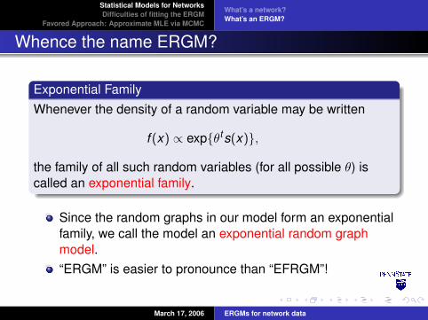
Whence the name ERGM?
Exponential FamilyWhenever the density of a random variable may be written
f (x) ∝ exp{θts(x)},
the family of all such random variables (for all possible θ) iscalled an exponential family.
Since the random graphs in our model form an exponentialfamily, we call the model an exponential random graphmodel.“ERGM” is easier to pronounce than “EFRGM”!
March 17, 2006 ERGMs for network data
Statistical Models for NetworksDifficulties of fitting the ERGM
Favored Approach: Approximate MLE via MCMC
What’s a network?What’s an ERGM?
Whence the name ERGM?
Exponential FamilyWhenever the density of a random variable may be written
f (x) ∝ exp{θts(x)},
the family of all such random variables (for all possible θ) iscalled an exponential family.
Since the random graphs in our model form an exponentialfamily, we call the model an exponential random graphmodel.“ERGM” is easier to pronounce than “EFRGM”!
March 17, 2006 ERGMs for network data

Statistical Models for NetworksDifficulties of fitting the ERGM
Favored Approach: Approximate MLE via MCMC
Why MLE is difficultChange Statistics and Maximum Pseudolikelihood
Maximum Likelihood Estimation
The model:
Pθ(X = x) =exp{θts(x)}
c(θ), where s(xobs) = 0
It follows that c(θ) is a normalizing “constant”:
c(θ) =∑
all possiblegraphs y
exp{θts(y)}.
Replacing s(x) by s(x)− s(xobs) leaves Pθ(X = x)unchanged; thus, we “recenter” s(x) so that s(xobs) = 0.
March 17, 2006 ERGMs for network data

Statistical Models for NetworksDifficulties of fitting the ERGM
Favored Approach: Approximate MLE via MCMC
Why MLE is difficultChange Statistics and Maximum Pseudolikelihood
Why it is difficult to find the MLE
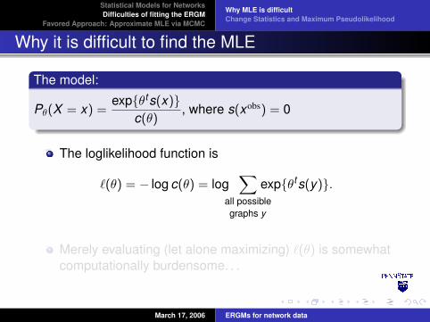
The model:
Pθ(X = x) =exp{θts(x)}
c(θ), where s(xobs) = 0
The loglikelihood function is
`(θ) = − log c(θ) = log∑
all possiblegraphs y
exp{θts(y)}.
Merely evaluating (let alone maximizing) `(θ) is somewhatcomputationally burdensome. . .
March 17, 2006 ERGMs for network data
Statistical Models for NetworksDifficulties of fitting the ERGM
Favored Approach: Approximate MLE via MCMC
Why MLE is difficultChange Statistics and Maximum Pseudolikelihood
Why it is difficult to find the MLE
The model:
Pθ(X = x) =exp{θts(x)}
c(θ), where s(xobs) = 0
The loglikelihood function is
`(θ) = − log c(θ) = log∑
all possiblegraphs y
exp{θts(y)}.
Merely evaluating (let alone maximizing) `(θ) is somewhatcomputationally burdensome. . .
March 17, 2006 ERGMs for network data

Statistical Models for NetworksDifficulties of fitting the ERGM
Favored Approach: Approximate MLE via MCMC
Why MLE is difficultChange Statistics and Maximum Pseudolikelihood
How burdensome?
7
8
7
11
8
8
7
8 8
9
7
11
9
8
11
7
9
9
10
7
7
9
89
9
7
9
7
9
7
7
8
9
7
For this undirected, 34-nodegraph, computing c(θ) directlyrequires summation of
7,547,924,849,643,082,704,483,109,161,976,537,781,833,842,440,832,880,856,752,412,600,491,248,324,784,297,704,172,253,450,355,317,535,082,936,750,061,527,689,799,541,169,259,849,585,265,122,868,502,865,392,087,298,790,653,952
terms.
March 17, 2006 ERGMs for network data

Statistical Models for NetworksDifficulties of fitting the ERGM
Favored Approach: Approximate MLE via MCMC
Why MLE is difficultChange Statistics and Maximum Pseudolikelihood
Conditional log-odds of an edge
Notation: For a network x and a pair (i , j) of nodes,
xij = 0 or 1, depending on whether there is an edgexc
ij denotes the status of all pairs in x other than (i , j)
x+ij denotes the same network as x but with xij = 1
x−ij denotes the same network as x but with xij = 0
Conditional on X cij = xc
ij , X has only two possible states,depending on whether Xij = 0 or Xij = 1.
March 17, 2006 ERGMs for network data

Statistical Models for NetworksDifficulties of fitting the ERGM
Favored Approach: Approximate MLE via MCMC
Why MLE is difficultChange Statistics and Maximum Pseudolikelihood
Conditional log-odds of an edge
Notation: For a network x and a pair (i , j) of nodes,
xij = 0 or 1, depending on whether there is an edgexc
ij denotes the status of all pairs in x other than (i , j)
x+ij denotes the same network as x but with xij = 1
x−ij denotes the same network as x but with xij = 0
Conditional on X cij = xc
ij , X has only two possible states,depending on whether Xij = 0 or Xij = 1.Let’s calculate the ratio of the two respective probabilities:
March 17, 2006 ERGMs for network data

Statistical Models for NetworksDifficulties of fitting the ERGM
Favored Approach: Approximate MLE via MCMC
Why MLE is difficultChange Statistics and Maximum Pseudolikelihood
Conditional log-odds of an edge
Notation: For a network x and a pair (i , j) of nodes,
xij = 0 or 1, depending on whether there is an edgexc
ij denotes the status of all pairs in x other than (i , j)
x+ij denotes the same network as x but with xij = 1
x−ij denotes the same network as x but with xij = 0
P(Xij = 1|X cij = xc
ij )
P(Xij = 0|X cij = xc
ij )=
exp{θts(x+ij )}
exp{θts(x−ij )}
March 17, 2006 ERGMs for network data

Statistical Models for NetworksDifficulties of fitting the ERGM
Favored Approach: Approximate MLE via MCMC
Why MLE is difficultChange Statistics and Maximum Pseudolikelihood
Conditional log-odds of an edge
Notation: For a network x and a pair (i , j) of nodes,
xij = 0 or 1, depending on whether there is an edgexc
ij denotes the status of all pairs in x other than (i , j)
x+ij denotes the same network as x but with xij = 1
x−ij denotes the same network as x but with xij = 0
P(Xij = 1|X cij = xc
ij )
P(Xij = 0|X cij = xc
ij )= exp{θt [s(x+
ij )− s(x−ij )]}
March 17, 2006 ERGMs for network data

Statistical Models for NetworksDifficulties of fitting the ERGM
Favored Approach: Approximate MLE via MCMC
Why MLE is difficultChange Statistics and Maximum Pseudolikelihood
Conditional log-odds of an edge
Notation: For a network x and a pair (i , j) of nodes,
xij = 0 or 1, depending on whether there is an edgexc
ij denotes the status of all pairs in x other than (i , j)
x+ij denotes the same network as x but with xij = 1
x−ij denotes the same network as x but with xij = 0
logP(Xij = 1|X c
ij = xcij )
P(Xij = 0|X cij = xc
ij )= θt [s(x+
ij )− s(x−ij )]
March 17, 2006 ERGMs for network data

Statistical Models for NetworksDifficulties of fitting the ERGM
Favored Approach: Approximate MLE via MCMC
Why MLE is difficultChange Statistics and Maximum Pseudolikelihood
Conditional log-odds of an edge
Notation: For a network x and a pair (i , j) of nodes,
∆(s(x))ij denotes the vector of change statistics,
∆(s(x))ij = s(x+ij )− s(x−ij ).
So ∆(s(x))ij is the conditional log-odds of edge (i , j).
logP(Xij = 1|X c
ij = xcij )
P(Xij = 0|X cij = xc
ij )= θt∆(s(x))ij
March 17, 2006 ERGMs for network data

Statistical Models for NetworksDifficulties of fitting the ERGM
Favored Approach: Approximate MLE via MCMC
Why MLE is difficultChange Statistics and Maximum Pseudolikelihood
Maximum Pseudolikelihood: Alternative to MLE?
What if we approximate the marginal P(Xij = 1) by theconditional P(Xij = 1|X c
ij = xcij )?
Then the Xij are independent with
logP(Xij = 1)
P(Xij = 0)= θt∆(s(xobs))ij ,
so we obtain θ̂ using simple logistic regression.Result: The maximum pseudolikelihood estimate.Unfortunately, little is known about the quality of MPLestimates.
March 17, 2006 ERGMs for network data

Statistical Models for NetworksDifficulties of fitting the ERGM
Favored Approach: Approximate MLE via MCMC
Why MLE is difficultChange Statistics and Maximum Pseudolikelihood
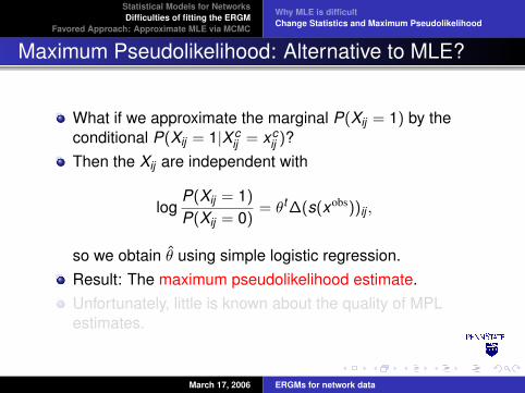
Maximum Pseudolikelihood: Alternative to MLE?
What if we approximate the marginal P(Xij = 1) by theconditional P(Xij = 1|X c
ij = xcij )?
Then the Xij are independent with
logP(Xij = 1)
P(Xij = 0)= θt∆(s(xobs))ij ,
so we obtain θ̂ using simple logistic regression.Result: The maximum pseudolikelihood estimate.Unfortunately, little is known about the quality of MPLestimates.
March 17, 2006 ERGMs for network data
Statistical Models for NetworksDifficulties of fitting the ERGM
Favored Approach: Approximate MLE via MCMC
Why MLE is difficultChange Statistics and Maximum Pseudolikelihood
Maximum Pseudolikelihood: Alternative to MLE?
What if we approximate the marginal P(Xij = 1) by theconditional P(Xij = 1|X c
ij = xcij )?
Then the Xij are independent with
logP(Xij = 1)
P(Xij = 0)= θt∆(s(xobs))ij ,
so we obtain θ̂ using simple logistic regression.Result: The maximum pseudolikelihood estimate.Unfortunately, little is known about the quality of MPLestimates.
March 17, 2006 ERGMs for network data

Statistical Models for NetworksDifficulties of fitting the ERGM
Favored Approach: Approximate MLE via MCMC
Law of Large Numbers to the RescueObtaining samples via MCMCA Numerical Example
MLE Revisited
Remember, c(θ) is really hard to compute.However, suppose we fix θ0. A bit of algebra shows that
E θ0
[exp
{(θ − θ0)
ts(X )}]
=c(θ)
c(θ0).
Thus, c(θ)/c(θ0) is the expectation of a function of arandom network, where the random behavior is governedby the known constant θ0.
March 17, 2006 ERGMs for network data

Statistical Models for NetworksDifficulties of fitting the ERGM
Favored Approach: Approximate MLE via MCMC
Law of Large Numbers to the RescueObtaining samples via MCMCA Numerical Example
Law of Large Numbers to the Rescue!
The LOLN suggests that we approximate an unknownpopulation mean by a sample mean.
Thus,
c(θ)/c(θ0) = E θ0
(exp
{(θ − θ0)
ts(X )})
≈ 1M
M∑i=1
exp{
(θ − θ0)ts(X (i))
},
where X (1), X (2), . . . , X (M) is a random sample of networks fromthe distribution defined by the ERGM with parameter θ0.
March 17, 2006 ERGMs for network data

Statistical Models for NetworksDifficulties of fitting the ERGM
Favored Approach: Approximate MLE via MCMC
Law of Large Numbers to the RescueObtaining samples via MCMCA Numerical Example
An approximate loglikelihood
Using the LOLN approximation, we find
`(θ)− `(θ0) = − logc(θ)
c(θ0)
= − log E θ0
(exp
{(θ − θ0)
ts(X )})
≈ − log1M
M∑i=1
exp{
(θ − θ0)ts(X (i))
}.
Now, all we need is a random sample of networks from Pθ0 .
March 17, 2006 ERGMs for network data

Statistical Models for NetworksDifficulties of fitting the ERGM
Favored Approach: Approximate MLE via MCMC
Law of Large Numbers to the RescueObtaining samples via MCMCA Numerical Example
Obtaining samples via MCMC
MCMC Idea:Simulate a discrete-time Markov chain whose stationarydistribution is the distribution we want to sample from.
We’ll discuss two common ways to run such a Markov chain:Gibbs samplingA Metropolis algorithm
March 17, 2006 ERGMs for network data

Statistical Models for NetworksDifficulties of fitting the ERGM
Favored Approach: Approximate MLE via MCMC
Law of Large Numbers to the RescueObtaining samples via MCMCA Numerical Example
Gibbs sampling
First, select a pair of nodes at random, say (i , j).Decide whether to set Xij = 0 or Xij = 1 at the next timestep according to the conditional distribution of Xij giventhe rest of the network (X c
ij ).Based on an earlier calculation, we obtain
Pθ0(Xij = 1|X cij = xc
ij ) =exp{θt
0∆(s(x))ij}(1 + exp{θt
0∆(s(x))ij}).
Note: To run the MCMC, the values of s(x+ij ) and s(x−ij ) are not
needed; only the difference ∆(s(x))ij matters.
March 17, 2006 ERGMs for network data

Statistical Models for NetworksDifficulties of fitting the ERGM
Favored Approach: Approximate MLE via MCMC
Law of Large Numbers to the RescueObtaining samples via MCMCA Numerical Example
Metropolis algorithm
First, select a pair of nodes at random, say (i , j).Calculate the ratio
π =P(Xij changes|X c
ij = xcij )
P(Xij does not change|X cij = xc
ij )
= exp{±θt0∆(s(x))ij}
Accept the change of Xij with probability min{1, π}.This scheme generally has better properties than Gibbssampling.
Note: To run the MCMC, the values of s(x+ij ) and s(x−ij ) are not
needed; only the difference ∆(s(x))ij matters.
March 17, 2006 ERGMs for network data

Statistical Models for NetworksDifficulties of fitting the ERGM
Favored Approach: Approximate MLE via MCMC
Law of Large Numbers to the RescueObtaining samples via MCMCA Numerical Example
How should θ0 be chosen?
Theoretically, the estimated value of `(θ)− `(θ0) convergesto the true value as the size of the MCMC sampleincreases, regardless of the value of θ0.However, this convergence can be agonizingly slow,especially if θ0 is not chosen close to the maximizer of thelikelihood.A choice that sometimes works is the MPLE (maximumpseudolikelihood estimate)
March 17, 2006 ERGMs for network data

Statistical Models for NetworksDifficulties of fitting the ERGM
Favored Approach: Approximate MLE via MCMC
Law of Large Numbers to the RescueObtaining samples via MCMCA Numerical Example
A numerical example
1 2
3
4
5
6
7
8
9
10
11
12
13
14
15
1617
==========================Summary of output==========================
Newton-Raphson iterations: 32MCMC sample of size 10000
Monte Carlo MLE Results:theta0 estimate s.e. p-value
match.grade 1.0706 1.4118 0.4988 0.0054dmatch.sex.0 1.0383 1.4660 0.7482 0.0522dmatch.sex.1 -0.9387 -0.7195 0.6767 0.2897triangle 1.1864 1.0389 0.5750 0.0732kstar1 9.3754 8.2408 5.3026 0.1226kstar2 -8.1424 -7.5155 4.4219 0.0916kstar3 5.2464 5.0092 3.3080 0.1324kstar4 -2.4226 -2.4512 1.8068 0.1773
Log likelihood of g: -78.52976
March 17, 2006 ERGMs for network data

Statistical Models for NetworksDifficulties of fitting the ERGM
Favored Approach: Approximate MLE via MCMC
Law of Large Numbers to the RescueObtaining samples via MCMCA Numerical Example
Some Useful References
Frank, O. and D. Strauss (1986), Markov graphs, JASAGeyer, C. J. and E. Thompson (1992), Constrained MonteCarlo maximum likelihood for dependent data, J. Roy. Stat.Soc. BHolland, P. W. and S. Leinhardt (1981), An exponentialfamily of probability distributions for directed graphs, JASASnijders, Tom A. B. (2002), Markov chain Monte Carloestimation of exponential random graph models, J. Soc.Struct.Strauss, D. and M. Ikeda (1990), Pseudolikelihoodestimation for social networks, JASAWasserman, S. and P. Pattison (1996), Logit models andlogistic regression for social networks: I. An introduction toMarkov graphs and p∗, Psychometrika
March 17, 2006 ERGMs for network data