Exponential inequalities and functional estimations - Docs at ISFA

Exponential inequalities and functionalestimations for weak dependent datas ;applications to dynamical systems

- Véronique MAUME-DESCHAMPS (Université Lyon 1, Laboratoire SAF)

2006.8

Laboratoire SAF – 50 Avenue Tony Garnier - 69366 Lyon cedex 07 http://www.isfa.fr/la_recherche

ccsd

-000

2245

3, v

ersi

on 1

- 9

Apr

200

6

EXPONENTIAL INEQUALITIES AND FUNCTIONAL

ESTIMATIONS FOR WEAK DEPENDENT DATAS ;

APPLICATIONS TO DYNAMICAL SYSTEMS.

V. MAUME-DESCHAMPS

Abstract. We estimate density and regression functions for weak de-pendant datas. Using an exponential inequality obtained in [DeP] and in[Mau2], we control the deviation between the estimator and the functionitself. These results are applied to a large class of dynamical systemsand lead to estimations of invariant densities and on the mapping itself.

Dynamical systems are widely used by scientists to modalize complexsystems ([ABST]). Therefore, estimating functions related to dynamicalsystems is crucial. Of particular interest are : the invariant density, themapping itself, the pressure function. We shall see that many dynamicalsystems have the same behavior as weak dependant processes (as defined in[DoLo]). We obtain results of deviation for regression functions and den-sities for weak dependant processes and apply these results to dynamicalsystems.In [Mau2] we gave an estimation (with control of the deviation) of the pres-sure function for some expanding maps of the interval. Results on the esti-mation of the invariant density for the same kind of maps where obtainedin [P] and stated in [Mae]. In this later article, results on the estimationof the mapping were also stated. These last two papers dealt with conver-gence in quadratic mean. Our goal here is, on one hand, to consider moregeneral dynamical systems : non uniformly hyperbolic maps on the interval,dynamics in higher dimension ... On the second hand, we obtain bounds onthe deviation between the estimator and the regression function as well asalmost sure convergence. Related results on the estimation of the regressionfunction may also be found in [FV] and [Mas] where strongly mixing pro-cesses are considered and almost everywhere convergence and asymptoticnormality are proved. Our aim is to provide an estimation of the deviationbetween the estimator and the regression function for a larger class of mix-ing processes and for regression functions that may have singularities.Before giving the precise definitions and results, let us state our main resultsinformally. We consider a weak dependant stationary process X0, ..., Xi, ...taking values in Σ ⊂ R

d. Our condition of weak dependence is with respectto a Banach space C of bounded functions on Σ (see Definition 1 below). Let(Yi)i∈N be a stationary process taking values in R and satisfying a conditionof weak dependence according with the process X0, ..., Xi, ... Consider the

2000 Mathematics Subject Classification. 37A50, 60E15, 37D20.Key words and phrases. Exponential inequalities, functional estimation, dynamical sys-

tems, weak dependance..

1

2 V. MAUME-DESCHAMPS

regression function r(x) = E(Yi | Xi = x), we shall assume some regularityon r (see Assumption 2 below). We shall also consider that the process(Xi)i∈N has a density f with respect to the Lebesgue measure m. f is ass-mued to have some regularity properties that allow localised singularities.Consider a non negative kernel K ∈ C satisfying Assumption 1 and the esti-mators (introduced in [R] and used for example in [P], [Mae], [FV], [Mas]) :

fn(x) =1

nh

n−1∑

i=0

K

(x−Xi

h

)gn(x) =

1

nh

n−1∑

i=0

YiK

(x−Xi

h

)

rn(x) =gn(x)

fn(x).(0.1)

Remark that fn(x) = 0 implies gn(x) = 0, in that case, we define rn(x) = 0.

Theorem. Assume some weak dependence condition on Xi and Yi (see Def-inition 1), assume that inf f > 0. There exists M > 0, L > 0, R > 0,0 ≤ β < 1, D > 0, γ′ > 0 such that, outside a set of measure less thanDhγ′

, for all n ∈ N⋆, for all t ∈ R

+, for all u ≥ Cth,

P(|fn(x) − f(x)| > t− uα) ≤ 2e1

e exp[−t2Mhβ+2n] if f is α regular

if r is bounded and α-regular,

P(|rn(x) − r(x)| > t− uα) ≤ e1

e

(2 exp[−t2Lnhβ+2] + exp[−L′nhβ+2]

),

if Yi ∈ L∞ and r is α-regular,

P(|rn(x) − r(x)| > t− uα) ≤ 2e1

e exp[−t2Lnhβ+2].

As a consequence, provided h = hn goes to zero and nhβ+2n = O(nε), ε > 0,

we obtain the following convergences provided r (and f) are α-regular :

• for m almost all x ∈ Σ, fn(x) converges to f(x) and rn(x) convergesto r(x) almost surely and in Lp for any 1 ≤ p,

• E

(∫

Σ|fn(x) − f(x)|dx

)and E

(∫

Σ|rn(x) − r(x)|

)go to zero.

• for almost all x ∈ Σ, for a < 12 , |gn(x) − g(x)| = OP(n−a) where gn

is either fn or rn and g is either f or r.

Using a “time inverted process” (as in [DeP, Mau2]), we deduce an es-timation of the invariant density and of the mapping itself for dynamicalsystems. Consider a discrete dynamical system from a “good class” (seeDefinition 1.4 for precise settings), denote by T the mapping and f the in-variant density of interest. Pick X0 at random with stationary law µ = fm

and let Xi = T i(X0). Consider a kernel K and fn as above, let rjn be the

estimator for Y ji = Xj

i+1 + εji , j = 1, . . . , d, Xji is the jth coordinate of Xi

and (εji )i∈N are independent stationary process with 0 mean, independent

of (Xi)i∈N. Let Tn be an estimator of the map T which has coordinates rjn.

Let ‖ ‖d be the sup norm in Rd, we have the following results.

Corollary. Assume that the dynamical is in the good class. There existsM > 0, L > 0, R > 0, 0 ≤ β ≤ 1, γ′ > 0 such that outside a set of measure

EXPONENTIAL INEQUALITIES AND FUNCTIONAL ESTIMATION 3

less than Rhγ′, for all t ∈ R


is f is regular P(|fn(x) − f(x)| > t− uα) ≤ 2e1

e exp[−t2Mhβ+2n](0.2)

P(‖Tn(x) − T (x)‖d > t− uα) ≤ 2e1

e exp[−t2Lhβ+2n].(0.3)


we obtain the following convergences :

• for m almost all x ∈ Σ, Tn(x) converges to T (x) almost surely and

in Lp for any 1 ≤ p, the same holds for fn(x) provided that f isα-regular.

• E

(∫

Σ‖Tn(x) − T (x)‖d

)go to zero, the same holds for fn(x) pro-

vided that f is α-regular.• for almost all x ∈ Σ, for a < 1

2 , |gn(x) − g(x)| = OP(n−a) where gn

is either fn or Tn and g is either f (provided it is α-regular) or T .

In a first section, we state our hypothesis on the process and the dynamicalsystems. We also give the precise results.The second section is devoted to the proofs.In the last section we provide examples of dynamical systems satisfying ourhypothesis. We also provide some simulations.

Contents

1. Hypothesis and statement of the results 31.1. Weak dependence 31.2. Regularity conditions 41.3. Main result 51.4. Dynamical systems 62. Proofs 72.1. Main ingredient : exponential inequality 72.2. Proof of Theorem 1.1 82.3. Dynamical systems and time reversed process 113. Examples and simulations 123.1. In dimension one : piecewise expanding maps 123.2. In dimension one : unimodal maps 193.3. Piecewise expanding maps in higher dimension 20References 22

1. Hypothesis and statement of the results

1.1. Weak dependence. As mentioned quickly in the introduction, weshall consider a class of weak mixing process with respect to a Banach spaceof bounded functions C. This functional definition of dependence is moregeneral than strong mixing used in [Mas] and [FV]. We shall see that itencounters a large class of dynamical systems (see also [DeP] for other ex-amples than dynamical systems). This kind of functional definition hasbeen introduced in [DoLo] and [DeP] for Lipschitz or BV functions (see also


[Mau2]).For simplicity, let Σ ⊂ R

d and (Xi)i∈N a process taking values in Σ. Ourproofs could probably be extended to sets Σ included in more general Banachspaces. In the following, ‖ ‖d denotes the sup norm on R

d : ‖(x1, . . . , xd)‖d =max(|xi|, i = 1, . . . , d).

Definition 1. Let C be a Banach space of bounded functions on Σ. Weconsider a norm on C of the form :

‖g‖C = ‖g‖∞ +C(g)

where C(·) is a semi-norm on C and ‖ · ‖∞ is the sup. norm on C. Let C1

be the “semi-ball” of functions g ∈ C such that C(g) ≤ 1. Let Mi be theσ-algebra generated by X0, . . . ,Xi. The C-mixing coefficients are :

ΦC(n) = sup{|E(Zg(Xi+n)) − E(Z)E(g(Xi+n))| i ∈ N, Z is

Mi − measurable and ‖Z‖1 ≤ 1, g ∈ C1}.(*)

The process (Xi)i∈N is C-weakly dependant if (ΦC(n))n∈N is summable.

Let Yi be a L1 stationary process, taking values in R. Let Mi be theσ-algebra generated by X0, Y0, . . . ,Xi, Yi. We shall say that (Xi)i∈N is C-weakly dependant with respect to (Yi)i∈N if the coefficients :

ΦC,(Yi)i∈N(n) = sup{|E(ZYi+ng(Xi+n)) − E(Z)E(Yi+ng(Xi+n))| i ∈ N, Z is

Mi − measurable and ‖Z‖1 ≤ 1, g ∈ C1},(**)

are summable.

Remark. Examples of spaces C that we shall consider are :

• the space of function with bounded variations, in that case, C(g) isthe total variation of g ;

• the space of Lipschitz (resp. Holder) functions, in that case, C(g) isthe Lipschitz (resp. Holder) constant ;

• the space of C1 function could also be considered, in that case, C(g)is the sup norm of g′.

1.2. Regularity conditions. We now state the conditions on the kernelK, the regression function r and the density function f .

Assumption 1. The kernel K is a nonnegative function in C (so it isbounded), with compact support D and with integral 1 :

∫

ΣKdm = 1.

For h > 0 and x ∈ Σ, let Kh,x(t) = K(

x−th

). We assume that there exists

0 ≤ β < 1 such that C(Kh,x) ≤C(K)

hβ .

Assumption 2. Consider a function g on Σ and 0 < α ≤ 1. Let Bg(u, h)be the set of points x such that

supd(x,y)<h

|g(x) − g(y)| > uα.

If g is a map from Σ to Σ, Bg(u, h) is the set of points x such that

supd(x,y)<h

‖g(x) − g(y)‖d > uα.


For any decreasing to zero sequences (un)n∈N and (hn)n∈N, let An = Bg(un, hn)

and BN =⋂

n≥N

⋃

p≥n

Ap.

We shall say that g is α-regular if for any sequence (un)n∈N decreasingto 0, for any sequence (hn)n∈N with hn = o(un), there exist constantsD(g),D′(g) > 0 and γ, γ′ > 0 such that m(BN ) ≤ D(g)hγ

N and m(AN ) ≤

D′(g)hγ′

N .

All our results are proved under the assumption that r and/or f areα-regular for some 0 < α ≤ 1.

Remarks. If g is α-Holder then it is α-regular with m(Bg(u, h)) = 0 for allu ≥ H(g)h with H(g) the Holder constant of g.If g is Lipschitz on Σ \{x} and discontinuous at x then m(Bg(u, h)) ≤ Cthd

for all u ≥ L(g)h where L(g) is the Lipschitz constant of g on Σ \ {x}.Functions of bounded variations satisfy this condition (see section 3).An α-regular function need not to be Holder everywhere but we control thepoints where this is not the case.

1.3. Main result. Let us state our main result for C-weak dependant pro-cess.

Theorem 1.1. Assume that (Xi)i∈N is a stationary process absolutely con-tinuous and is C-weakly dependant with respect to (Yi)i∈N, (Yi)i∈N is a sta-tionary process taking values in R. Let r be the regression function (r =E(Yi|Xi)) and f , the density function, we assume that inf f > 0. Then thereexists M > 0, L > 0, L′ > 0, R > 0, a set Au,h such that for all n ∈ N

⋆, for

all t ∈ R+, for x 6∈ Au,h, for all u ≥ h · Diam(D), m(Au,h) ≤ Rhγ′

,if f is α-regular,

(1.1) P(|fn(x) − f(x)| > t− uα) ≤ 2e1

e exp[−t2Mnhβ+2],

if r is α-regular and bounded,(1.2)

P(|rn(x) − r(x)| > t− uα) ≤ e1

e

(2 exp[−t2Lnhβ+2] + exp[−L′nhβ+2]

),

if r is α-regular and Yi ∈ L∞,

(1.3) P(|rn(x) − r(x)| > t− uα) ≤ 2e1

e exp[−t2Lnhβ+2].



• for m almost all x ∈ Σ, rn(x) converges to r(x) almost surely and in

Lp for any 1 ≤ p, the same holds for fn(x) provided f is α-regular.

• E

(∫

Σ|rn(x) − r(x)|

)goes to zero, the same holds for fn(x) provided

f is α-regular.• for almost all x ∈ Σ, for a < 1

2 , |rn(x) − r(x)| = OP(n−a), the same

holds for fn(x) provided f is α-regular.


1.4. Dynamical systems. We turn now to our main motivation : dynami-cal systems. Consider a dynamical system (Σ, T , µ). That is, T maps Σ intoitself, µ is a T -invariant probability measure on Σ, absolutely continuouswith respect to the Lebesgue measure m. We assume that the dynamicalsystem satisfy the following mixing property : for all ϕ ∈ L1(µ), ψ ∈ C,

(1.4)

∣∣∣∣∣∣

∫

Σ

ψ · ϕ ◦ T ndµ −

∫

Σ

ψdµ

∫

Σ

ϕdµ

∣∣∣∣∣∣≤ Φ(n)‖ϕ‖1‖ψ‖C ,

with Φ(n) summable.

Definition 2. A dynamical system (Σ, T , µ) is of the good class if

(1) Σ is a bounded subset of Rd,

(2) the map T : Σ → Σ is α-regular,(3) the invariant density f (µ = fm) verify inf f > 0,(4) it satisfy the mixing property (1.4).

We shall also assume that the Banach space C is regular in the sense thatfor any ϕ ∈ C, there exists R(ϕ) ∈ R such that

(1.5) ‖ϕ+R(ϕ)‖∞ ≤ C(ϕ).

We consider the stationary process taking values in Σ : Xi = T i with lawµ and Yi = Xi+1 + εi where the εi are L1 independent random vectors,with independent coordinates, identically distributed random variables with0 mean and independent on (Xi)i∈N. Then T is the regression function

T (x) = E(Yi|Xi = x). Let rjn is the estimator for Y j

i = Xji+1 +εji , defined by

(0.1), j = 1, . . . , d, Xji is the jth coordinate ofXi and εji is the jth coordiante

of εi. We shall denote Tn the estimator of T which has coordinates rjn.

Theorem 1.1 applied in the context of dynamical systems gives the followingresult.

Corollary 1.2. Let T be a dynamical system of the good class, assumethat the Banach space C is regular. There exists M > 0, L > 0, R > 0,0 ≤ β ≤ 1, γ′ > 0 such that outside a set of measure less than Rhγ′

, for allt ∈ R


P(‖Tn(x) − T (x)‖d > t− uα) ≤ 2de1

e exp[−t2Lhβ+2n]

P(|fn(x) − f(x)| > t− uα) ≤ 2e1

e exp[−t2Mhβ+2n] if f is α-regular.



• for m almost all Tn(x) converges to T (x) x ∈ Σ, fn(x) converges to

f(x) almost surely and in Lp for any 1 ≤ p, if f is α-regular, fn(x)converges to f(x) almost surely and in Lp for any 1 ≤ p,

• E

(∫

Σ‖Tn(x) − T (x)‖d

)go to zero, if f is α-regular,

E

(∫

Σ|fn(x) − f(x)|dx

)go to zero.


is either fn or Tn and g is either f (provided f is α-regular) or T .


2. Proofs

Let us now prove the results stated in the above section. The main in-gredient is an exponential inequality that has been obtained in [DeP] in thecase C = BV , and in [Mau2] for more general spaces C.

2.1. Main ingredient : exponential inequality.

Proposition 2.1. Let (Xi)i∈N be a C-weakly mixing process. Let the coeffi-cients ΦC(k) be defined by (*). For ϕ ∈ C, p ≥ 2, define

Sn(ϕ) =n∑

i=1

ϕ(Xi)

and

bi,n = ΦC(0)

(n−i∑

k=0

ΦC(k)

)‖ϕ(Xi) − E(ϕ(Xi))‖p

2C(ϕ).

For any p ≥ 2, we have the inequality :

‖Sn(ϕ) − E(Sn(ϕ))‖p ≤

(2pΦC(0)

n∑

i=1

bi,n

) 1

2

≤ C(ϕ)

(2p

n−1∑

k=0

(n− k)ΦC(k)

) 1

2

.(2.1)

As a consequence, we obtain

P (|Sn(ϕ) − E(Sn(ϕ))| > t)

≤ e1

e exp

(−t2

2e(C(ϕ))2ΦC(0)∑n−1

k=0(n − k)ΦC(k)

).(2.2)

Applying Proposition 2.1 to the function φ = K will provide an expo-

nential inequality for fn. The proof of Proposition 2.1 may be found in[Mau2] (Proposition 1.1), see also [DeP] for a version of this propositionwith C = BV . In order to have an exponential inequality for gn, we needthe following result.

Proposition 2.2. Let (Xi)i∈N be a C-weakly mixing process with respect to(Yi)i∈N. Let the coefficients ΦC,(Yi)i∈N

(k) be defined by (**). For ϕ ∈ C,p ≥ 2, define

Sn(ϕ) =

n∑

i=1

Yiϕ(Xi)

and

bi,n = ΦC(0),(Yi)i∈N

(n−i∑

k=0

ΦC,(Yi)i∈N(k)

)‖Yiϕ(Xi) − E(Yiϕ(Xi))‖p

2C(ϕ).


For any p ≥ 2, we have the inequality :

‖Sn(ϕ) − E(Sn(ϕ))‖p ≤

(2p

n∑

i=1

bi,n

) 1

2

≤ C(ϕ)

(2pΦC,(Yi)i∈N

(0)n−1∑

k=0

(n− k)ΦC,(Yi)i∈N(k)

) 1

2

.(2.3)

As a consequence, we obtain

P (|Sn(ϕ) − E(Sn(ϕ))| > t)

≤ e1

e exp

(−t2

2e(C(ϕ))2ΦC(0),(Yi)i∈N

∑n−1k=0(n − k)ΦC,(Yi)i∈N

(k)

).(2.4)

Proof. Proposition 2.2 is proved as Proposition 1.1 in [Mau2] using the vari-

able Zi = Yiϕ(Xi) − E(Yiϕ(Xi)) for which we control ‖E(Zk|Mi)‖∞ withthe coefficients ΦC,(Yi)i∈N

(k − i), for k ≥ i. �

2.2. Proof of Theorem 1.1. As already mentioned, the proof of Theorem1.1 uses Propositions 2.1 and 2.2 applied to ϕ = K. This gives a control on

the deviation between fn(x) (resp. gn(x)) and E(fn(x)) (resp. E(gn(x))).

Then it remains to see to that E(fn(x)) is close to f(x). In order to obtainthe result for the regression function, we deduce from the previous results

a control on the deviation between rn(x) andE(gn(x))

E(fn(x)), then we prove that

E(gn(x))

E(fn(x))is close to r(x). To this aim, we begin with two lemmas.

Lemma 2.3. We assume that the density function f is α-regular. For allu ≥ hdiam(D) =: k, if x 6∈ Bf (u, k) we have :

|E(fn(x)) − f(x)| ≤ uα.

Proof. We have :

E(fn(x)) =

∫

DK(y)f(x− hy)dm(y).

If x 6∈ Bf (u, k) then for y ∈ D,

|f(x) − f(x− hy)| ≤ uα.

The result follows from the fact that the integral of K is 1. �

Lemma 2.4. We assume that the regression function r is α-regular. Forall u ≥ hdiam(D) =: k, if x 6∈ Br(u, k) we have :

∣∣∣∣∣E(gn(x))

E(fn(x))− r(x)

∣∣∣∣∣ ≤ uα.

Proof. We have :

E(gn(x))

E(fn(x))=

∫

Dr(x− yh)K(x)f(x− yh)dm(y)∫

DK(x)f(x− yh)dm(y)

.


If x 6∈ Br(u, k) then for y ∈ D,

|r(x) − r(x− hy)| ≤ uα

and the result follows. �

Proof of Theorem 1.1. Proposition 2.1 applied to ϕ(t) = K(

x−th

)gives : for

all t > 0, for all n ∈ N, for all x ∈ Σ,

P(|fn(x) − E(fn(x))| > t) ≤ e1

e exp

(−

t2nhβ+2

2eRΦC(0)C(K)

),

where R is the smallest positive number such that

n−1∑

k=0

(n− k)ΦC(k) ≤ Rn.

This together with Lemma 2.3 gives (1.1) for x 6∈ Bf (u, k) (k = hdiam(D)).In order to obtain the estimation for the regression function r, we applyProposition 2.2 to ϕ(t) = K

(x−th

). We obtain :

P(|gn(x) − E(gn(x)| > t) ≤ e1

e exp

(−

t2nhβ+2

2eR′ΦC,(Yi)i∈N(0)C(K)

),

where R′ is the smallest positive number such that

n−1∑

k=0

(n− k)ΦC,(Yi)i∈N(k) ≤ R′n.

Now, for any t > 0,

P

(∣∣∣∣∣rn(x) −E(gn(x))

E(fn(x))

∣∣∣∣∣ > t

)≤ P

(|gn(x) − E(gn(x)| >

t

2E(fn(x)

)

+ P

(|fn(x) − E(fn(x)| >

t

2E(fn(x)rn(x)−1

).

Now, assume that Yi ∈ L∞, we remark that |rn(x)| ≤ ‖Yi‖∞ =: ymax thus :

P

(∣∣∣∣∣rn(x) −E(gn(x))

E(fn(x))

∣∣∣∣∣ > t

)≤ P

(|gn(x) − E(gn(x))| >

t

2inf f

)

+ P

(|fn(x) − E(fn(x))| >

t

2

inf f

ymax

).

Propositions 2.1 and 2.2 give :

P

(∣∣∣∣∣rn(x) −E(gn(x))

E(fn(x))

∣∣∣∣∣ > t

)≤ 2e

1

e exp[−Ct2hβ+2n]

where

C = max

((inf f)2

8eR′ΦC,(Yi)i∈N(0)C(K)

,(inf f)2

8eRΦC(0)C(K)y2max

).


Lemma 2.4 gives (1.3) for x 6∈ Br(u, k). Let Ah = Bf (u, k) ∪ Br(u, k), thefirst part of Theorem 1.1 is now proved for x 6∈ Ah if Yi ∈ L∞.If we don’t assume Yi ∈ L∞, but r is bounded by rmax, we write :

P

(∣∣∣∣∣rn(x) −E(gn(x))

E(fn(x))

∣∣∣∣∣ > t

)≤ P

(|gn(x) − E(gn(x))| >

t

2fn(x)

)

+P

|fn(x) − E(fn(x))| >

t

2fn(x)

[E(gn(x))

E(fn(x))

]−1

≤ P

(|gn(x) − E(gn(x))| >

t

4inf f

)+ P

(|fn(x) − E(fn(x))| >

t

4

inf f

rmax

)

+P

(fn(x) <

inf f

2

).

Propositions 2.1 and 2.2 give :

P

(|rn(x) −

E(gn(x))

E(fn(x))| > t

)≤ e

1

e

[2 exp[−C ′t2hβ+2n] + exp[−C ′′nhβ+2]

],

where C ′ and C ′′ may be expressed in terms of inf f , rmax, R, R′,ΦC(0),ΦC,(Yi)i∈N

(0), C(K). Then (1.2) follows as above for x 6∈ Ah.Let us conclude with the almost everywhere and Lp convergence, for all1 ≤ p. Let us begin with the convergence in Lp(m). We fix 1 ≤ p. We

remark that since the kernel K is bounded, so is fn : sup(fn) ≤ sup Kh . Also,

if x 6∈ Bf (u, ε) then f(x) ≤ 1+uα

εd . Let Et,u(x) be the event

Et,u(x) = {|fn(x) − f(x)| > t− uα},

we have :∫

|fn(x) − f(x)|pdP =

∫

Et,u(x)|fn(x) − f(x)|pdP

+

∫

[Et,u(x)]c|fn(x) − f(x)|pdP

≤ P(Et,u(x))

(1 + uα

diam(D)h+

supK

h

)p

+ (t− uα)p

≤Ct

hpexp[−Ct2hβn] + (t− uα)p.

Take u such that uα = 1ln n , t = 2uα and h = hn = O( 1

nξ ) with 0 < ξ < 1β+2 .

Then for x 6∈ An = Bf (un, hn), there exists 0 < κ < 1 and constantsC1, C2 > 0 such that :

‖fn(x) − f(x)‖pp ≤ C1e

−C2nκ

+

(1

lnn

)p

.

Thus, ‖fn(x) − f(x)‖p goes to zero for x 6∈ BN = ∩n≥N ∪p≥n Ap and

m(BN ) = O(hγN ). We conclude that for almost all x ∈ Σ, fn(x) goes to

f(x) in Lp(m).


The proof of the almost everywhere convergence is in the same spirit. Con-sider a sequence tm decreasing to 0, for x ∈ Σ,

P({fn(x) 6→ f(x)}) ≤ limm→∞

limN→∞

∑

n≥N

P({|fn(x) − f(x)| > tm}).

Take h = hn = O( 1nξ ) with 0 < ξ < 1

β+2 then

limN→∞

∑

n≥N

P({|fn(x) − f(x)| > tm}) = 0

provided tm > uα with uα > Cthn and x 6∈ Bu,hn , we take u = un = 1lnn and

An = Bun,hn, for x 6∈ ∩N ∪n≥N An =: B, fn(x) goes to f(x) and m(B) = 0.The proofs of Lp(m) and almost everywhere convergence for rn follow thesame lines.Finally, to prove the bound for the convergence in probability, recall thatun = OP(n−a) if and only if

limM→∞

lim supn→∞

P(na|un| > M) = 0.

Following the same lines as above, we prove that for g either f or r and gn

either fn or rn,

limM→∞

lim supn→∞

P(na|gn(x) − g(x)| > M) = 0

for a < 12 , x 6∈ B = ∩n≥0 ∪p≥n Ap and m(B) = 0. �

Let us show how we can apply the above result to dynamical systems.

2.3. Dynamical systems and time reversed process. It turns out that,in general, the process (Xi)i∈N associated to a dynamical system (Σ, T , µ)is not weakly dependent. Nevertheless the condition of weak dependenceis satisfied for a “time reversed process” whose law is the same as (Xi)i∈N.Indeed, Condition 1.4 together with the fact that the space C is regular(recall (1.5)) gives (see [DeP] or [Mau2] for the details) : for all i ∈ N, forψ ∈ C1, ϕ ∈ L1, ‖ϕ‖1 ≤ 1,

(2.5) |Cov(ψ(Xi), ϕ(Xn+i))| ≤ 2Φ(n).

So that, if we consider the process (Xi)i∈N defined by

(X0, . . . , Xn)Law= (Xn, . . . ,X0) ∀n ∈ N,

it is C-weakly dependent.Recall that Yi = Xi+1 + εi with (εi)i∈N independent random vectors, withindependent coordinates, of zero mean, which is also independent of (Xi)i∈N.In order to estimate the regression function E(Yi|Xi) = T , we shall estimateseparately each coordinates of Xi+1. Let

gjn(x) =

1

nh

n−1∑

i=0

Y ji K

(x−Xi

h

)

=1

nh

n−1∑

i=0

Xji+1K

(x−Xi

h

)+

1

nh

n−1∑

i=0

εjiK

(x−Xi

h

).


Equation (2.5) implies also that (Xi)i∈N is C-weakly dependant with respect

to each (Xji+1)i∈N, and also to each (εji ), j = 1, . . . , d. We obtain inequalities

(1.3) separately for the two parts of gjn(x) and then the two parts of rj

n(x).Then we deduce Corollary 1.2.

3. Examples and simulations

We shall now give some examples of discrete dynamical systems satisfying(2.5), such that T is α-regular, admits a unique invariant density (withrespect to the Lebesgue measure), f which may be also α-regular.There is a large class of dynamical systems satisfying (2.5), we refer tothe literature on dynamical systems : [Y1, Y2, Mau1, Li, Col, BuMau1,BuMau2, LiSV, Bro] and many other, see [Ba] for a review on these topics.Below we consider Lasota-Yorke maps, unimodal maps, piecewise expandingmaps in higher dimension. Our results should also apply for hyperbolic mapsbut a more intricate study on the invariant density is required.

3.1. In dimension one : piecewise expanding maps. We shall considerpiecewise expanding maps or “Lasota-Yorke” maps. Consider I = [0, 1],partitioned into subintervals Ij. On the interior of the Ij’s, the map T isC2, uniformly expanding |T ′| ≥ λ > 1, and continuous on the closure of theIj’s. Under additional conditions of mixing or covering (see below), it is wellknown ([Bro, LiSV, Li, Col]) that T admits a unique absolutely continuousinvariant measure whose density f belongs to the space BV of functions ofbounded variations.Before we give precisely the hypothesis on the map, we prove that functionsof bounded variations are regular. We shall denote m the Lebesgue measureon I.Recall that a function g on I belongs to BV if

∨g = sup

n∑

i=0

|g(ai) − g(ai+1)| <∞

where the supremum is taken over all the finite subdivisions of I ; a0 = 0 <a1 < · · · < an+1 = 1, then

∨g is the total variation of g.

Lemma 3.1. Let g belongs to BV . Then for any sequences (un)n∈N and(hn)n∈N decreasing to zero with h2−α

n ≤ u2n, 0 < α < 2, let Bg(u, h) be the

set of points x such that

supd(x,y)<h

|g(x) − g(y)| > u,

An = Bg(un, hn) and BN =⋂

n≥N

⋃

p≥n

Ap.

Then

m(BN ) ≤ 3(∨g)h

α2

N and m(An) ≤ 2(∨g)hn

un

Proof. Let x0 = inf BN and x1 such that 0 ≤ x1 − x0 ≤ hN and x1 ∈ BN .Then x1 belongs to Ap for infinitely many p ≥ N . In particular, thereexists p1 ≥ N and x2 with |x1 − x2| ≤ hp1

and |g(x1) − g(x2)| ≥ up1. Set


x0 = x1,0, x1 = x1,1 and x2 = x1,2. We construct sequences (maybe finite)(xi,0, xi,1, xi,2) and (pi) such that :

(1) pi ≥ N for all i ≥ 1,(2) xi,0 ≤ min(xi,1, xi,2) ; xi+1,0 ≥ max(xi,1, xi,2), xi,1 ∈ Api

,(3) |xi,0 − xi,1| ≤ hpi−1

for all i ≥ 1, with the convention that hp0= hN ,

(4) |xi,1 − xi,2| ≤ hpifor all i ≥ 1,

(5) |g(xi,1) − g(xi,2)| ≥ upifor all i ≥ 1,

(6) BN ⊂⋃

i≥1 Ji with Ji = [ai, bi+hpi−1], [ai, bi] = [xi,0, xi,1]∪[xi,1, xi,2].

If xi,0, xi,1, xi,2 are already constructed, let xi+1,0 = inf[x ∈ BN , x ≥max(xi,1, xi,2) + hpi

]. Now, there exists xi+1,1 ∈ BN with 0 ≤ xi+1,1 −xi+1,0 ≤ hpi

. Since xi+1,1 ∈ BN , there exists pi+1 ≥ pi and xi+1,2 with|xi+1,1 − xi+1,2| ≤ hpi+1

and |g(xi+1,1) − g(xi+1,2)| ≥ upi+1. In that way, all

the points of BN smaller than max(xi+1,2, xi+1,1) + hpi+1are in

i+1⋃

j=1

Jj . The

construction stops when {x ∈ BN , x ≥ max(xi,1, xi,2) + hpi} is empty.

As a consequence of this construction, we get :∑

i≥1

upi≤∨g remark that the Ji’s are disjoint,

m(BN ) ≤ 3∑

i≥0

hpi.

Now, using Cauchy-Schwartz inequality,

∑

i≥0

hpi≤

∑

i≥1

h2pi

upi

1

2

·

∑

i≥1

upi

1

2

≤(∨

g) 1

2

· hα2

N

∑

i≥1

h2−αpi

upi

1

2

≤∨g · h

α2

N recall that h2−αn ≤ u2

n.

Finally, we have proven : m(BN ) ≤ 3(∨g)h

α2

N .The estimation on the measure of An is much simpler. We may cover An byballs of radius 2hn, centered on points x such that supd(x,y)<hn

|g(x)−g(y)| >un. Then, m(An) ≤ 2 · k · hn where k is the number of such balls. Now,∨g ≥ k · un, thus k ≤

∨g

un. �

3.1.1. Finite number of pieces. This subsection is devoted to Lasota-Yorkemaps with a finite number of intervals of monotonicity. The main differencesbetween infinite and finite pieces are some additional technical assumptionsin the infinite case.We consider the following conditions that may be found in [Col, Li].

Assumption 3.


(1) The partition (Ii)i=1,...r of I is finite, denote by Pk the partition of

invertibility of T k.(2) T satisfies the covering property : for all k ∈ N, there exists N(k)

such that for all P ∈ Pk,

TN(k)P = [0, 1].

(3) On each Ii, the map T is C2.

The following result is standard and may be found in ([Col, Li, Ba]).

Theorem 3.2. Under Assumptions 3, the map T admits a unique absolutelyinvariant probability measure, its density f belongs to BV and inf f > 0.Moreover, if µ = fm is this invariant probability measure, then (1.4) issatisfied with C = BV and Φ(n) = γn, 0 < γ < 1 : there exists 0 < γ < 1,C > 0, such that for any ψ ∈ BV and ϕ ∈ L1(µ), for any n ∈ N,

∣∣∣∣∣∣

∫

I


∫

I

ψdµ

∫

I

ϕdµ

∣∣∣∣∣∣≤ Cγn‖ϕ‖1‖ψ‖BV .

We already know that f is regular by Lemma 3.1. In order to have theconditions of Corollary 1.2, it remains to prove that T is regular. This isindeed clear because T is piecewise C2, with finitely many points of disconti-nuity. As a consequence, for any sequences (un)n∈N and (hn)n∈N decreasingto zero with hN ≤ uN

sup |T ′| ,

m(AN ) ≤

p∑

i=1

|gi| · hN

where we have denoted by xi, i = 1, . . . , p the points of discontinuity, andgi the gap at xi : gi = |T (x−i ) − T (x+

i )|. Moreover, as soon as uN ≤ inf gi,we have that An ⊃ An+1, so BN = AN and we have the required control onthe measure of AN .Thus, Corollary 1.2 applies and we get the following result.

Corollary 3.3. Let T satisfies Assumption 3, let K be a Kernel belonging

to BV , let fN and TN be the estimators of f and T . For all 0 < α < 1, hereexists M > 0, L > 0, R > 0, such that outside a set of measure less thanRhα, for all t ∈ R


P(|fn(x) − f(x)| > t− uα) ≤ 2e1

e exp[−t2Mnh2](3.1)

P(|Tn(x) − T (x)| > t− uα) ≤ 2e1

e exp[−t2Lnh2].(3.2)

As a consequence, provided h = hn goes to zero and nh2n = O(nε), ε > 0,


• for m almost all x ∈ Σ, fn(x) converges to f(x) and Tn(x) convergesto T (x) almost surely and in Lp for any 1 ≤ p,

• E

(∫

I|fn(x) − f(x)|dx

)and E

(∫

I|Tn(x) − T (x)|

)go to zero.


is either fn or Tn and g is either f or T .


Proof. We apply Corollary 1.2. Since the Kernel K belongs to BV , we maytake β = 0. Also, with our hypothesis, T and f are in BV so they areregular according to Lemma 3.1. �

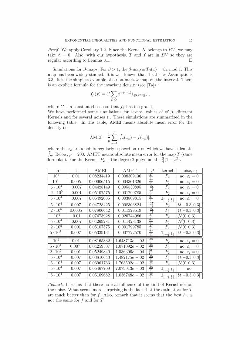
Simulations for β-maps. For β > 1, the β-map is Tβ(x) = βx mod 1. Thismap has been widely studied. It is well known that it satisfies Assumptions3.3. It is the simplest example of a non-markov map on the interval. Thereis an explicit formula for the invariant density (see [Ta]) :

fβ(x) = C∑

i≥0

β−(i+1)1[0,T i1](x),

where C is a constant chosen so that fβ has integral 1.We have performed some simulations for several values of of β, differentKernels and for several noises εi. These simulations are summarized in thefollowing table. In this table, AMEf means absolute mean error for thedensity i.e.

AMEf =1

p

p∑

k=1

|fn(xk) − f(xk)|,

where the xk are p points regularly espaced on I on which we have calculate

fn. Below, p = 200. AMET means absolute mean error for the map T (sameformulae). For the Kernel, P2 is the degree 2 polynomial : 3

4(1 − x2).

n h AMEf AMET β kernel noise, εi104 0.01 0.08234419 0.008309136 27

11 P2 no, εi = 0

104 0.005 0.09906515 0.004301326 2711 P2 no, εi = 0

5 · 104 0.007 0.04428149 0.005530895 2711 P2 no, εi = 0

2 · 105 0.001 0.05107575 0.001799785 2711 P2 no, εi = 0

5 · 104 0.007 0.05492035 0.003809815 2711 1[− 1

2, 12] no, εi = 0

5 · 104 0.007 0.04728425 0.008303824 2711 P2 U [−0.3, 0.3]

2 · 105 0.0005 0.07806642 0.011328519 2711 P2 U [−0.3, 0.3]

104 0.01 0.07473928 0.020744986 2711 P2 N (0, 0.3)

5 · 104 0.007 0.04269281 0.011423138 2711 P2 N (0, 0.3)

2 · 105 0.001 0.05107575 0.001799785 2711 P2 N (0, 0.3)

5 · 104 0.007 0.05329131 0.007722570 2711 1[− 1

2, 12] U [−0.3, 0.3]

104 0.01 0.08165332 1.648713e − 02 4611 P2 no, εi = 0

5 · 104 0.007 0.04259507 1.071092e − 02 4611 P2 no, εi = 0

2 · 105 0.001 0.05249840 1.536396e − 04 4611 P2 no, εi = 0

5 · 104 0.007 0.03810643 1.482175e − 02 4611 P2 U [−0.3, 0.3]

5 · 104 0.007 0.03961733 1.763502e − 02 4611 P2 N (0, 0.3)

5 · 104 0.007 0.05467709 7.079913e − 03 4611 1[− 1

2, 12] no

5 · 104 0.007 0.05109682 1.036748e − 02 4611 1[− 1

2, 12] U [−0.3, 0.3]

Remark. It seems that there no real influence of the kind of Kernel nor onthe noise. What seems more surprising is the fact that the estimators for Tare much better than for f . Also, remark that it seems that the best hn isnot the same for f and for T .


The graphics below correspond to β = 2711 , K = 1[− 1

2, 12], εi ; U [−0.2, 0.2],

n = 50000 and h = 0.007.

3.1.2. Infinite number of pieces. If the number of pieces is infinite, their aremany different settings leading to existence and uniqueness of an absolutelycontinuous invariant probability measure which is exponentially mixing. Letus cite [Bro, LiSV]. We will consider the conditions of Liverani-Saussol-Vaienti [LiSV] in a restricted case (our potential is |T ′|−1, they considermore general potential). These conditions are the following.

Assumption 4. (1) There is a countable partition (Ij)j∈N of I into in-tervals. On each Ij, the map T is monotonic and C2, it is continuous

on each Ij. Denote by P the partition (Ij)j∈N and by Pk the parti-

tion of monotonicity of T k.

(2)1

|T ′|∈ BV and

∑

P∈P

sup1

|T ′|<∞.

(3) The partition P is generating.(4) The map T is covering, which means, in the infinite case, that for

any n ∈ N, for any P ∈ Pn, I may covered by a finite number of


subintervals of TNP :

∀n ∈ N, ∀P ∈ Pn, ∃N, ∃ finite J ⊂ PN

∨{P} /

⋃

Q∈J

TNQ = X.

Remark. The condition1

|T ′|∈ BV is satisfied provided that T has the

bounded distortion property :

supP∈P

supx∈P

|T ′′(x)|

|T ′(x)|2<∞

and that∑

P∈P

sup1

|T ′|<∞.

The following result has been proved in a general setting in [LiSV] and in[Bro] under the condition of bounded distortion.

Theorem 3.4. Under Assumptions 4, the map T admits a unique absolutelyinvariant probability measure, its density f belongs to BV and inf f > 0.Moreover, if µ = fm is this invariant probability measure, then (1.4) issatisfied with C = BV and Φ(n) = γn, 0 < γ < 1 : there exists 0 < γ < 1,C > 0, such that for any ψ ∈ BV and ϕ ∈ L1(µ), for any n ∈ N,

∣∣∣∣∣∣

∫

I


∫

I

ψdµ

∫

I

ϕdµ

∣∣∣∣∣∣≤ Cγn‖ϕ‖1‖ψ‖BV .

Lemma 3.5. The map T satisfying Assumptions 4 is regular.

Idea of the proof. This is a simple consequence of the fact that T is piecewise

C2 (thus piecewise C1) and that∑

P∈P

sup1

|T ′|<∞. �

There are several natural examples of dynamical systems satisfying As-sumptions 4. Let us cite the Gauss map :

T (x) =1

x−

⌊1

x

⌋

which appears in the continuous fractions decomposition ([Bro]) and in anal-ysis a gcd algorithms ([V]). An natural extension of these systems are“Japanese systems” or α-Gauss maps : for 0 < α ≤ 1,

Tα(x) =

∣∣∣∣1

x

∣∣∣∣−⌊∣∣∣∣

1

x

∣∣∣∣+ 1 − α

⌋,

Tα maps the interval [α − 1, α] into itself. See [BoDaV] for a description ofthese systems as well as an application to analysis of generalized Euclidianalgorithms. The maps Tα satisfy Asumption 4 for 0 < α ≤ 1.

Corollary 3.6. Let T satisfies Assumption 4, let K be a Kernel belonging

to BV , let fN and TN be the estimators of f and T . For all 0 < α < 1, here


exists M > 0, L > 0, R > 0, such that outside a set of measure less thanRhα, for all t ∈ R


P(|fn(x) − f(x)| > t− uα) ≤ 2e1

e exp[−t2Mnh2](3.3)

P(|Tn(x) − T (x)| > t− uα) ≤ 2e1

e exp[−t2Lnh2].(3.4)



• for m almost all x ∈ I, fn(x) converges to f(x) and Tn(x) convergesto T (x) almost surely and in Lp for any 1 ≤ p,

• E

(∫

I|fn(x) − f(x)|dx

)and E

(∫

I|Tn(x) − T (x)|

)go to zero.

• for almost all x ∈ I, for a < 12 , |gn(x) − g(x)| = OP(n−a) where gn

is either fn or Tn and g is either f or T .

The following graphics are for the Gauss map T (x) = 1x (mod 1) for which

it is known that the unique invariant probability density is f(x) = 1log 2

11+x .

We have performed simulations with n = 50000, h = 0.009 and the noiseεi ; U [−0.2, 0.2]. Over 800 points, we get EMEf = 0.05046933, AMET =0.05141938, if we restrict to points in [0.2, 1] we get AMET = 0.01439787.


3.2. In dimension one : unimodal maps. Let I = [−1, 1] and f : I → Ibe a C2 unimodal map (i.e., f is increasing on [−1, 0], decreasing on [0, 1])satisfying f ′′(0) 6= 0, and,

(H1) There are 0 < α < 1, K > 1, and λ ≤ λ ≤ 4 with e2α < λ, and

supI |f′| ≤ λK < 8 so that

(i) |(fn)′(f(0))| ≥ λn for all n ∈ N and λ = limn→∞ |(fn)′(f(0))|1/n.(ii) |fn(0)| ≥ e−αn, for all n ≥ 1.(H2) For each small enough δ > 0, there is M = M(δ) ∈ N+ for which

(i) If x, . . . , fM−1(x) /∈ (−δ, δ) then |(fM )′(x)| ≥ λM ; (ii) For each n, if

x, . . . , fn−1(x) /∈ (−δ, δ) and fn(x) ∈ (−δ, δ), then |(fn)′(x)| ≥ λn.(H3) f is topologically mixing on [f2(0), f(0)], that is for any two open setsU , V ⊂ I, there exists N ∈ N such that ∀n ≥ N , T−nU ∩ V 6= ∅.

Examples of unimodal maps satisfying (H1)–(H3) are quadratic maps1 − a · x2 for a positive measure set of parameters a. (See e.g. [BeCa]).The following theorem is obtained in two steps. First, it is proven thatunimodal maps satisfying (H1)–(H3) are conjugated to a kind of hyperbolicmarkov maps called Young towers (see [Y1, KeNo]). Then the estimation onthe speed of mixing is obtained on the tower ([BuMau1]). Let us emphasizethe fact that the kind a mixing we need (namely 1.4) and especially the factthat ‖ϕ‖1 appears, is not obtained in [Y1, KeNo] (a form with the ‖ϕ‖∞was obtained there).

Theorem 3.7. Let T be a unimodal map satisfying (H1)–(H3). The mapT admits a unique absolutely invariant probability measure with density fsatisfying inf

[f2(0),f(0)]f > 0. Moreover, if µ = fm is this invariant probability

measure, then (1.4) is satisfied with C the space Lip of Lipschitz functionson I and Φ(n) = γn, 0 < γ < 1 : there exists 0 < γ < 1, C > 0, such thatfor any ψ ∈ Lip and ϕ ∈ L1(µ), for any n ∈ N,

∣∣∣∣∣∣

∫

I

ψ · ϕ ◦ T ndµ−

∫

I

ψdµ

∫

I

ϕdµ

∣∣∣∣∣∣≤ Cγn‖ϕ‖1‖ψ‖Lip.

This is clear that T is 1-regular : for well chosen εn and un, the setsAN and BN are empty because T is C2. Nevertheless, it is known that theinvariant density is very irregular (see [Y2, KeNo]). With a more intricatestudy, we should probably prove that f is also regular. Here, we restrictourselves to the estimation of T .Since the invariant measure has its support in S = [f2(0), f(0)], our esti-mates are valid only for x ∈ S.

Corollary 3.8. Let T be a unimodal map satisfying (H1)–(H3), let K be a

Kernel belonging to Lip, let TN be the estimator of T . There exists M > 0,L > 0, R > 0, such that outside a subset of S, of measure less than Rh, forall t ∈ R


P(|Tn(x) − T (x)| > t− u) ≤ 2e1

e exp[−t2Lh2n].




• for m almost all x ∈ S, Tn(x) converges to T (x) almost surely andin Lp for any 1 ≤ p,

• E

(∫

S|Tn(x) − T (x)|

)go to zero.

• for almost all x ∈ S, for a < 12 , |Tn(x) − T (x)| = OP(n−a).

The following graphics are for the map T (x) = 3.8 ∗ x ∗ (1 − x). Wehave performed simulations with n = 50000, h = 0.01 and the noise εi ;

U [−0.2, 0.2]. Over 154 points in S, we get AMET = 0.004114143.

3.3. Piecewise expanding maps in higher dimension. These are gen-eralisations of Lasota-Yorke maps in higher dimension. These maps havebeen studied in [Bu4, BuPaS, Bu1, Bu2, Bu5, Cow, GoBo, Sau] from var-ious point of view. The control of the speed of mixing may be found in[BuMau1, BuMau2], the strategy is as for unimodal maps : the map is con-jugated to a “Young tower”.The setting is the following. (X,Z, T ) will be a piecewise invertible map,i.e.:

• X =⋃

Z∈Z Z is a locally connected compact subset of Rd.

• Z is a finite collection of pairwise disjoint, bounded and open subsetsof X, each with a non-empty boundary. Let Y =

⋃Z∈Z Z.

• T : Y → X is a map such that each restriction T |Z, Z ∈ Z, coincideswith the restriction of a homeomorphism TZ : U → V with U, V opensets such that U ⊃ Z, V ⊃ T (Z).

T will be assumed to be non-contracting, i.e., such that for all x, y in thesame element Z ∈ Z, d(Tx, Ty) ≥ d(x, y). Also Z will be assumed tobe generating, i.e., limn→∞ diam(Zn) = 0 where Zn denotes the set of n-cylinders, i.e., the non-empty sets of the form:

[A0 . . . An−1] := A0 ∩ · · · ∩ T−n+1An−1

forA0, . . . , An−1 ∈ Z. Finally the boundary of the partition, ∂Z =⋃

Z∈Z ∂Z,

will play an important role in our analysis. In particular, we shall assume“small boundary pressure” (see below), a fundamental condition which al-ready appeared in [Bu4, Bu5, BuPaS]. To formulate the crucial “small


boundary pressure” condition, we need first some definitions.The topological pressure [DGS] of a subset S of X is:

P (S, T ) = lim supn→∞

1

nlog

∑

A∈Zn

A∩S 6=∅

g(n)(A)

where g(n)(A) = supx∈A g(x)g(Tx) . . . g(Tn−1x), g = |detT ′|−1.

The small boundary pressure condition is:

P (∂Z, T ) < P (X,T ).

This inequality is satisfied in many cases. In particular, if T is expanding

and X is a Riemannian manifold and the weight is |detT ′(x)|−1 or close toit, then it is satisfied: (i) in dimension 1, in all cases; (ii) in dimension 2, ifT is piecewise real analytic [Bu5, Ts1]; (iii) in arbitrary dimension, for allpiecewise affine T [Ts2] or for generic T [Bu3, Cow].A basic example is given by the multidimensional β-transformations [Bu1],i.e., maps T : [0, 1]d → [0, 1]d, T (x) = B(x) mod Z

d with B an expandingaffine map on R

d. Let us summarize our hypothesis on T .

Assumption 5. Let (X,Z, T, g) be a weighted piecewise invertible dynam-ical system. Assume that:

• T is expanding, i.e., there is some λ > 1 such that for all x, y in thesame element of Z, d(Tx, Ty) ≥ λ · d(x, y);

• g = |detT ′|−1 is Holder continuous with exponent γ and is positivelylower bounded.

• the boundary pressure is small: P (∂Z, T ) < P (X,T ).• T is topologically mixing.

LetK(f) = maxZ∈Z supx 6=y∈Z|f(x)−f(y)|

d(x,y)γ where γ is some Holder exponent

of g.

Theorem 3.9. [BuMau1] Let T satisfy Assumption 5. Then, T admitsa unique invariant measure µ, absolutely continuous w.r.t. the Lebesguemeausre m. This measure is exponentially mixing :

∣∣∣∣∫

Xϕ ◦ T n · ψ dµ −

∫

Xϕdµ

∫

Xψ dµ

∣∣∣∣ ≤ C · ‖ϕ‖Cγ (X) · ‖ψ‖L1 κn.

with constants C < ∞ and κ < 1 depending only on (X,Z, T, g), for anymeasurable functions ϕ,ψ : X → R such that ψ is bounded and ϕ is γ-Holdercontinuous.

This is clear that T is 1-regular because it is piecewise C1. Nevertheless, itis known that the invariant density has discontinuities on ∂[T n(Zn)] . Witha more intricate study, we should probably prove that f is also regular.Here, we restrict ourselves to the estimate of T .

Corollary 3.10. Let T satisfy Asumption 5, let K be a γ-Holder Kernel,

let TN be the estimator of T . There exists M > 0, L > 0, R > 0, such thatoutside a set of measure less than Rh, for all t ∈ R


P(|Tn(x) − T (x)| > t− u) ≤ 2e1

e exp[−t2Lhγ+2n].


As a consequence, provided h = hn goes to zero and nhγ+2n = O(nε), ε > 0,


• for m almost all x ∈ X, Tn(x) converges to T (x) almost surely andin Lp for any 1 ≤ p,

• E

(∫

X|Tn(x) − T (x)|

)go to zero.

• for almost all x ∈ X, for a < 12 , |Tn(x) − T (x)| = OP(n−a).

We have performed some simulations for T (x) = Bx mod Z2, with B the

matrix (2.5 3.44.6 3.2

)

Below are the histograms for diffx (resp. diffy), the difference beetween

the x (resp. y) coordinate of T and the x (resp. y) coordinate of Tn, overa grid of 100 times 100 points in [0, 1]2. The Kernel is K = 1

41[−1,1]×[−1,1],there is no noise, εi = 0, n = 66668 and h = 0.004. The AME for thecoordinate x is 0.01882885, for the coordinate y, the AME is 0.06723186.

Remark (Anosov maps). Our technics should also apply to estimate theinvariant density and the application T for Anosov maps for which there ex-ists an invariant measure absolutely continuous with respect to the Lebesguemeasure. A more intricate study could also lead results of the same kind forAxiom A diffeomorphisms.

References

[ABST] H. D Abarbanel, R. Brown, J. J. Sidorowich, L. S. Tsimring, The analysis ofobserved chaotic data in physical systems. Rev. Modern Phys. 65 (1993), no.4, 1331-1392.

[Ba] V. Baladi Positive Transfer Operators and Decay of Correlations, Book, Ad-vanced Series in Nonlinear Dynamics, Vol 16, World Scientific, Singapore(2000).

[BeCa] M. Benedicks, L. Carleson On iterations of 1 − ax2 on (-1,1) Ann. of Math.(2), 122, (1985), 1–25

[Bro] A. Broise, Transformations dilatantes de l’intervalle et theoremes limites.

Etudes spectrales d’operateurs de transfert et applications. Asterisque 1996,no. 238, 1–109.


[BoDaV] J. Bourdon, B. Daireaux, B. Vallee Dynamical Analysis of a-Euclidean Algo-rithms, Journal of Algorithms, 44, (1), (2002), pp. 246-285.

[Bu1] J. Buzzi Intrinsic ergodicity of affine maps in [0, 1]d. Monatsh. Math. 124 (1997),97–118.

[Bu2] J. Buzzi Markov extensions for multi-dimensional dynamical systems. Israel J.Math. 112 (1999), 357–380.

[Bu3] J. Buzzi Absolutely continuous invariant measures for generic piecewise affineand expanding maps Int. J. Chaos & Bif. (1999), 9 (9), 1743-1750.

[Bu4] J. Buzzi Thermodynamical formalism for picewise invertible maps : absolutelycontinuous invariant measures as equilibrium states in Smooth Ergodic Theoryand its Applications (Seattle, WA 1999), Proceedings of Symposia in PureMathematics 69, AMS, RI, (2001), 749–783.

[Bu5] J. Buzzi Absolutely continuous invariant probability measures for arbitrary ex-panding piecewise R-analytic mappings of the plane. Ergodic Theory Dynam.Systems 20 (2000), 697–708.

[BuMau1] J. Buzzi, V. Maume-Deschamps Decay of correlations on towers for potentialswith summable variation, Discrete and Continuous Dynamical Systems, 12,(2005), no 4, 639-656.

[BuMau2] J. Buzzi, V. Maume-Deschamps Decay of correlations for piecewise invertiblemaps in higher dimensions, Israel J. Math. 131 (2002), 203-220.

[BuPaS] J. Buzzi, F. Paccaut, B. Schmitt, Conformal measures for multidimensionalpiecewise invertible maps. Ergodic Theory Dynam. Systems 21 (2001), no. 4,1035–1049.

[Col] P. Collet, Some ergodic properties of maps of the interval. Dynamical systems(Temuco, 1991/1992), 55–91, Travaux en Cours, 52, Hermann, Paris, 1996.

[CMarS] P. Collet, S. Martinez, B. Schmitt, Exponential inequalities for dynamical mea-sures of expanding maps of the interval. Probab. Theory Related Fields 123(2002), no. 3, 301–322.

[Cow] W. Cowieson, Piecewise smooth expanding maps in Rd, Ph.D. Thesis, U.C.L.A.,

Berkeley (see http://math.usc.edu/˜cowieson).[DeDo] J. Dedecker, P. Doukhan, A new covariance inequality and applications. Sto-

chastic Process. Appl. 106 (2003), no. 1, 63–80.[DGS] M. Denker, C. Grillenberger, K. Sygmund Ergodic theory on compact spaces.

Lecture notes in mathematics 527, Springer, Berlin, 1976.[DeP] J. Dedecker, C. Prieur, New dependence coefficients. Examples and applications

to statistics. To appear in Probab. Theory and Relat. Fields.[DoLo] P. Doukhan, S. Louhichi, m A new weak dependence condition and applications

to moment inequalities. Stochastic Process. Appl. 84 (1999), no. 2, 313–342.[FV] F. Ferraty, P. Vieu, Nonparametric models for functional data, with applications

in regression, time series prediction and curves discrimination. J. of Nonpara-metric Statistics, 16, 111-125, (2004).

[GoBo] P. Gora, A. Boyarsky Absolutely continuous invariant measures for piecewiseexpanding C2 transformation in RN . Israel J. Math. 67 (1989), 272–286.

[KeNo] G. Keller, T. Nowicki Spectral theory, zeta functions and the distribution ofperiodic points for Collet-Eckmann maps. Comm. Math. Phys. (1992), 149, 1,31-69.

[Li] C. Liverani, Decay of correlations for piecewise expanding maps. J. Statist.Phys. 78 (1995), no. 3-4, 1111–1129.

[LiSV] C. Liverani, B. Saussol, S. Vaienti, Conformal measure and decay of correlationfor covering weighted systems. Ergodic Theory Dynam. Systems 18 (1998), no.6, 1399–1420.

[Mae] J. Maes Estimation non parametrique pour des processus dynamiques dilatants.C. R. Acad. Sci. Paris Ser. I Math. 330 (2000), no. 9, 831–834.

[Mas] E. Masry Nonparametric regression estimation for dependent functional data:asymptotic normality. Stochastic Processes and their Applications, 115, (2005),155–177.


[Mau1] V. Maume-Deschamps Projective metrics and mixing properties on towers,Trans. A.M.S. 353, (2001), 8, 3371-3389.

[Mau2] V. Maume-Deschamps Exponential inequalities and estima-tion of conditional probabilities. dans Dependence in probabil-ity and statistics, Lect. notes in Stat., Springer, Vol. 187Bertail, Patrice; Doukhan, Paul; Soulier, Philippe (Eds.), (2006).http://www.springer.com/sgw/cda/frontpage/0,11855,1-0-22-122342957-0,00.html?referer=www.springe

[P] C. Prieur Density estimation for one-dimensional dynamical systems. ESAIMProbab. Statist. 5 (2001), 51–76.

[R] M. Rosenblatt, Conditional probability density and regression estimators. Mul-tivariate Analysis, II (Proc. Second Internat. Sympos., Dayton, Ohio, 1968),(1969), pp. 25–31 Academic Press, New York.

[Sau] B. Saussol Absolutely continuous invariant measures for multidimensional ex-panding maps. Israel J. Math. 116 (2000), 223–248.

[Ta] Y. Takahashi, β-transformations and symbolic dynamics. Proceedings of theSecond Japan-USSR Symposium on Probability Theory (Kyoto, 1972), pp.455–464. Lecture Notes in Math., Vol. 330, Springer, Berlin, (1973).

[Ts1] M. Tsujii, Absolutely continuous invariant measures for piecewise real-analyticexpanding maps on the plane. Comm. Math. Phys. 208 (2000), 605–622.

[Ts2] M. Tsujii, Absolutely continuous invariant measures for expanding piecewiselinear maps Invent. Math. (to appear).

[Ts3] M. Tsujii, Piecewise Expanding maps on the plane with singular ergodic prop-erties. Ergod. th. and Dynam. Syst. (to appear).

[V] B. Vallee Digits and continuants in Euclidean algorithms. Ergodic versus Taube-rian theorems. J. Theor. Nombres Bordeaux 12 (2000), no. 2, 531–570.

[Y1] L.-S. Young Statistical properties of dynamical systems with some hyperbolicity.Ann. of Math. (2) (1998), 147, 3, 585-650.

[Y2] L.-S. Young Recurrence times and rates of mixing. Israel J. Math. 110 (1999),153–188.

Universite de Bourgogne B.P. 47870 21078 Dijon Cedex FRANCE

E-mail address: [email protected]

Documents

Exponential inequalities and functional estimations - Docs at ISFA