Exploratorydataanalysisoftheelectricalenergydemandinthetimedomain

inGreece

Hristos Tyralis*, Georgios Karakatsanis, Katerina Tzouka, Nikos Mamassis

* Department of Water Resources and Environmental Engineering, School of Civil

Engineering, National Technical University of Athens, Iroon Polythechniou 5, GR-157 80

Zografou, Greece, (montchrister@gmail.com)

Abstract: The electrical energy demand (EED) in Greece for the time period 2002-2016

is investigated. The aim of the study is to introduce a framework for the exploratory data

analysis (EDA) of the EED in the time domain. To this end, the EED at the hourly, daily,

seasonal and annual time scale along with the mean daily temperature and the Gross

Domestic Product (GDP) of Greece are visualized. The forecast of the EED provided by the

Greek Independent Power Transmission Operator (IPTO) is also visualized and is

compared with the actual EED. Furthermore, the EED pricing system is visualized. The

results of the study in general confirm and summarize the conclusions of previous

relevant studies in Greece, each one treating a single topic and covering shorter and

earlier time periods. Furthermore, some unexpected patterns are observed, which if not

considered carefully could result to dubious models. Therefore, it is shown that the EDA

of the EED in the time domain coupled with weather-, climate-related and socio-economic

variables is essential for the building of a model for the short-, medium- and long-term

EED forecasting, something not highlighted in the literature.

Keywords: electrical energy demand; energy forecasting; exploratory data analysis;

Greece; Gross Domestic Product; temperature

1. Introduction

1.1 Electrical energy demand forecasting

Electrical Energy Demand (EED) forecasting regards the prediction of hourly, daily,

weekly, monthly, and annual values of the system demand and peak demand [1]. EED

forecasts are classified into three categories, according to the horizon of the forecast.

Short-term forecasts usually range from one hour to one week, medium-term forecasts

usually range from one week to one year, and long-term forecasts are usually applied to

time intervals longer than a year [2], albeit in the absence of a standard the time intervals

may differ [3]. The short-term variation of the EED seems to depend mostly on

2

fluctuations of the weather (e.g. [4]). On the other hand, concerning the long-term

forecasting, there is a strong correlation between the EED and socio-economic variables,

with a significant amount of studies examining their possible causal relationships (e.g. [5,

6]). Therefore, the investigation of the EED at various time scales and its relationship with

weather- and climate-related and socio-economic variables is essential for its forecast.

The modelling and forecasting of the EED is important for formulating a sustainable

energy policy [7]. The EED forecasting can serve short-, medium- and long-term

objectives. Short-term forecasting is necessary for the daily operation (energy

transactions, unit commitment, security analysis, and economic dispatch) of generation

and distribution systems [2,8]. Medium-term forecasting is used by electrical energy

producers and resellers for maintenance planning of grids and market researching [2].

Long-term forecasting is used for planning the expansion of the generation and

distribution system [2,8].

Before modelling the EED in the time domain, it is important to understand its

behaviour. To understand time series data a frequent approach adopted by data scientists

is the exploratory data analysis (EDA) which emphasizes the graphical representation of

the data. Based on the classical book of Tukey [9], Behrens and Yu [10] mention that in

the context of EDA, data analysts and scientists work interactively in a cyclical process of

pattern extraction and pattern interpretation. The aim is to complement the model

building based on the findings of the EDA [11]. EDA also aims “to find the unexpected”,

e.g. to identify misleading patterns and to develop rich descriptions [10]. Chatfield [12] in

a critique of Tukey’s [9] work, adds a second objective of the EDA, i.e. the model

formulation. Chatfield [12] and Behrens and Yu [10] also point out that in many studies

the EDA is undervalued or neglected leading to the implementation of useless models

(following the famous Box’s [13] quote that “all models are wrong, some are useful”).

1.2 Greek and international literature review on the electrical energy demand analysis

In this study, the EED in the Greek Interconnected Electric System (GIES) is investigated.

The GIES is part of the Greek Electric System (GES). The GIES consists of subsystems of

generation, distribution and consumption of electrical energy. The GIES extends to the

mainland Greece and the islands close to the mainland [14]. The GES also includes the

electric systems in remote islands. The Independent Power Transmission Operator

(IPTO) operates, maintains and develops the GES. The Operator of Electricity Market

3

(OEM) operates the process of the exchange between electricity producers and electricity

consumers. The Regulatory Authority for Energy (RAE) supervises the OEM [15].

Several studies can be found, which analyse the energy demand in Greece. Amongst

them, there exist studies of special interest for the present case study because their results

are comparable to the present analysis. In most cases, these studies treat a single topic or

they are applied to a short time interval. Psiloglou et al. [16] investigated the electrical

energy demand of Athens for the period 1997-2001, and examined issues such as the

relationship of the EED with the weather (e.g. the temperature) and socio-economic

variables. Mirasgedis et al. [17] present a similar analysis about the EED in Greece for the

time period 1993-2002. Pappas et al. [18] visualize the EED in Greece for the time period

2004-2005, and use the results to fit a stochastic model. Regarding the long-term

forecasting, Ekonomou [19], Kalampalikas and Pilavachi [20], and Dagoumas and Kitsios

[21] examine the relationship between the energy demand and socio-economic variables.

Additional published studies about the energy demand (or the EED) in Greece and in

neighbouring Cyprus (with a Greek culture) include issues related to the energy market

[15], the spatial analysis of the EED [22,23], the relationship between the energy demand

and the economic activity [6,24–29], the relationship between the energy demand and

climatic or geological variables [30–32], the renewable sources [33–35], the energy

consumption for domestic use [36,37], the study of power system production [14], the

exergy [38], the energy policy [39] and energy issues regarding Cyprus [4,40] or Greek

regions [41].

The international literature also includes several studies concerning the EED analyses

in the time domain. Such analyses include the examination of the causality relationship

between the electrical energy consumption and the Gross Domestic Product (GDP) [42–

44], the short- and long-term forecasting of energy demand and production [45–51], the

relationship between the energy demand and the economic activity or socio-economic

factors [7,52–55], the relationship between the energy demand and climatic or geological

variables [56–59], the relationship between the energy demand and both socio-economic

activities and climatic variables [60,61], the energy demand in various sectors of the

economy [62,63], the distribution of the energy demand at different time scales [2,8], the

domestic energy demand [64,65], the operation of grids [66] and many other topics. A

review of the literature is presented in Jebaraj and Iniyan [67], Suganthi and Samuel [68]

and recently in Hong and Fan [3] and Ghalehkhondabi et al. [69], while, regarding the

4

causal relationship between electricity consumption and economic growth, Payne [5]

presents a survey of the empirical literature. Furthermore, Aggarwal et al. [70] present a

literature review on the related subject of electrical energy price forecasting.

1.3 Aim of the study

In Section 1.1, the importance of the EED time series modelling and forecasting was

emphasized. Furthermore, the importance of performing an EDA before modelling a time

series was shown. An accurate forecast depends on the implementation of a useful model,

which in turn depends on the correct description and use of available data. In Section 1.2,

an extended literature on the EED analysis in the time domain was presented in which

each paper treats a single or a couple of topics, regarding the relationship between the

EED and other variables.

The present study has been motivated by the fact that in the EED forecasting literature

little importance has been given to the integrated analysis of the data. Google Scholar

returns 45 results when using simultaneously the terms “exploratory data analysis” and

“energy forecasting”, four results when using “exploratory data analysis” and “electricity

forecasting” and 12 results when using the terms “exploratory data analysis” and “energy

demand forecasting” (access: Saturday, August 13, 2016). Among them, the studies of

Dudek [71], Hippert and Pedreira [72], Narayan et al. [73] and Vaghefi et al. [74] were

distinguished, however their EDA still remains limited.

The number of original techniques for EED forecasting is still countable, i.e. within 100

and their applications in the literature have been exhausted [3]. Hong and Fan [3] also

mention that a “universally best technique simply does not exist”. Furthermore, they define

three steps for EED forecasting, i.e. “understanding of the business needs first, then

analysing the data, and going through a trial and-error process, to figure out which is the

best technique for a specific dataset in a specific jurisdiction”. Consequently, the selection

of the best technique depends on the problem at hand, therefore the analysis of the data

is crucial.

The R package MEFM (abbreviation for Monash Electricity Forecasting Model) based

on Hyndman and Fan [1] models the EED as a function of observed EED, temperatures

and seasonal socio-economic data and delivers a forecast using a combination of

stochastic and machine learning methods. The package is flexible in the sense that various

types of socio-economic data can be given as inputs. We emphasize that the forecast does

5

not depend only on observed EED data. Indeed, in many studies, there is an attempt to

apply time series models (from the families of autoregressive moving average (ARMA)

models, [3]) to the data and use the fitted models to forecast the EED. However, neglecting

the information from weather and climate data and socio-economic variables may be

misleading for specific purposes (e.g. see Section 3.1.3, 3.1.4 and 3.1.9(2) in Hong and Fan

[3] however, ARMAX models, which are generalizations of ARMA models, may include

exogenous variables). The forecasts constitute an important part of the energy policy of a

state, thus the procedure of forecasting must not be taken light-heartedly.

In this study, the EED in Greece for the time period 2002-2015 is investigated. The EED

is visualized at the hourly, daily, seasonal and annual time scale along with the mean daily

temperature, the GDP of Greece, the forecast of the EED provided by the IPTO and the EED

pricing system. Furthermore, the forecast is compared with the actual EED. The aim of our

study is to deliver a complete description of the data and to suggest a methodological EDA

framework for application to EED forecasting techniques emphasising visualization

methods.

We think that if we wish to deliver a valid short-, medium- or long-term forecast of the

EED and avoid the implementation of useless models, we must at least perform an EDA

similar to that of the present study. Before resorting to general models, possible hidden

patterns must be revealed, which if not modelled sufficiently, they may invalidate the

accuracy of the forecast. Furthermore, an interdisciplinary approach to the exploitation

of all available information is also needed. Using the knowledge across several scientific

fields may help to interpret the results of the visualization.

The results of our study confirm and summarize the conclusions of previous relevant

studies in Greece, each one treating a single topic and covering shorter and earlier time

periods. Some unexpected patterns are also revealed. The results of the analysis will be

used in the development of an electrical energy forecasting system, which will be a part

of a framework for optimal planning of a large-scale hybrid renewable energy system in

which hydropower plays the dominant role.

The raw and wrangled data and code of the present study as well as additional Figures,

associated with the present study but not included here for brevity, are available in

Tyralis et al. [75]. The interested reader can use it to reproduce our analysis.

6

2. Dataandmethods

In Section 2, the data and methods used in the subsequent Sections are presented. EED,

price, GDP and temperature data are used. The cleaning of the raw data is presented in

Tyralis et al. [75]. In Table 1, the variables examined in the next Sections are summarized,

along with their availability during the study time period. The IPTO [76] provided the

weekly ahead load forecast.

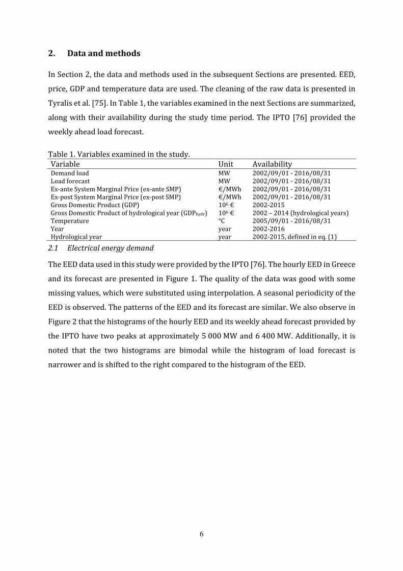
Table 1. Variables examined in the study. Variable Unit Availability Demand load MW 2002/09/01 - 2016/08/31 Load forecast MW 2002/09/01 - 2016/08/31 Ex-ante System Marginal Price (ex-ante SMP) €/MWh 2002/09/01 - 2016/08/31 Ex-post System Marginal Price (ex-post SMP) €/MWh 2002/09/01 - 2016/08/31 Gross Domestic Product (GDP) 106 € 2002-2015 Gross Domestic Product of hydrological year (GDPhydr) 106 € 2002 – 2014 (hydrological years) Temperature °C 2005/09/01 - 2016/08/31 Year year 2002-2016 Hydrological year year 2002-2015, defined in eq. (1)

2.1 Electrical energy demand

The EED data used in this study were provided by the IPTO [76]. The hourly EED in Greece

and its forecast are presented in Figure 1. The quality of the data was good with some

missing values, which were substituted using interpolation. A seasonal periodicity of the

EED is observed. The patterns of the EED and its forecast are similar. We also observe in

Figure 2 that the histograms of the hourly EED and its weekly ahead forecast provided by

the IPTO have two peaks at approximately 5 000 MW and 6 400 MW. Additionally, it is

noted that the two histograms are bimodal while the histogram of load forecast is

narrower and is shifted to the right compared to the histogram of the EED.

7

Figure 1. Hourly EED (top) and weekly ahead hourly forecasted load in Greece, provided by the IPTO (bottom) for the time period 2002/09/01 - 2016/08/31 (Data source: IPTO [76]).

Figure 2. Histogram of the hourly EED (left) and the weekly ahead hourly forecasted load in Greece, provided by the IPTO (right) for the time period 2002/09/01 - 2016/08/31.

2.2 Gross Domestic Product

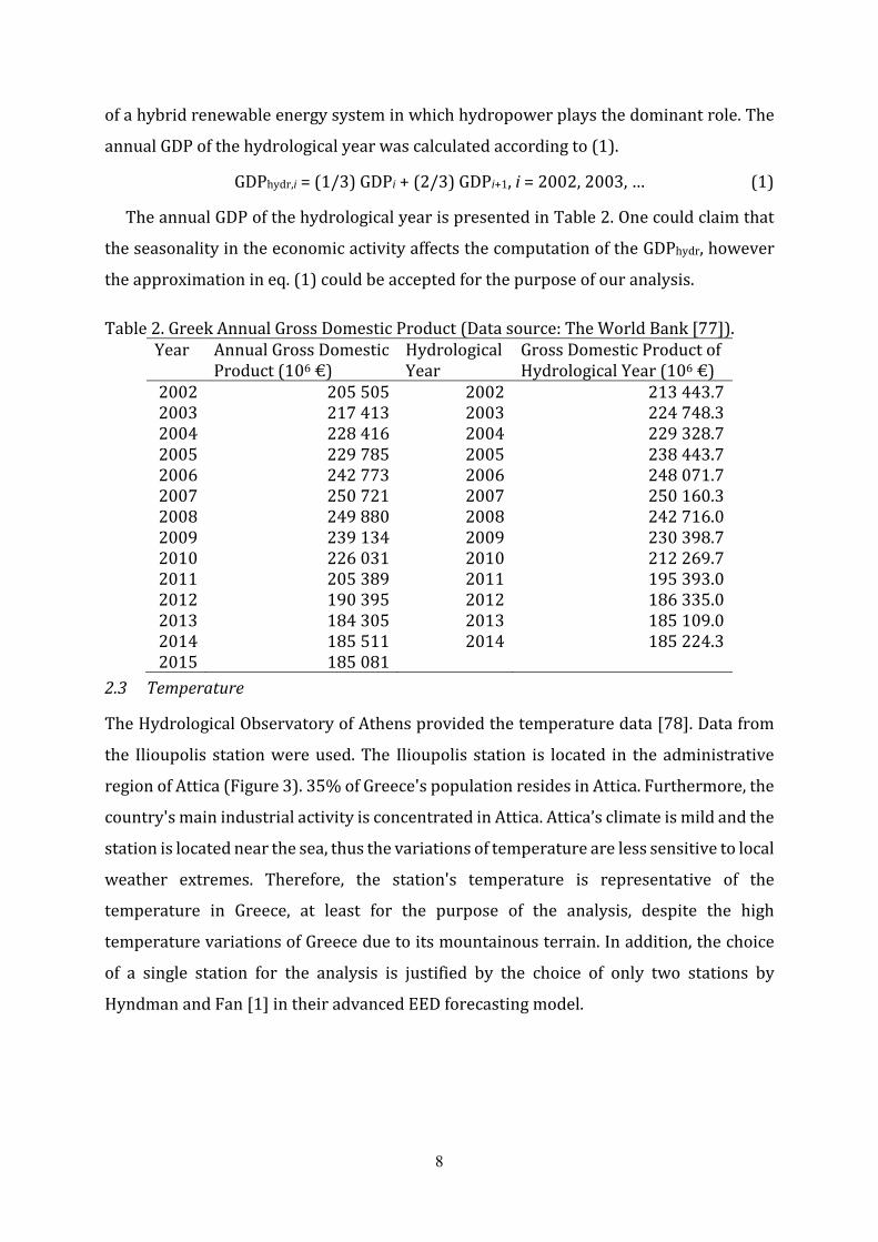
The World Bank [77] provided the annual GDP of Greece (see Table 2). In this study, the

hydrological year was defined, as the period between September 1st of one year and

August 31st of the next. The present analysis will use the hydrological year as the

reference time period because the results of the study will be used for optimal planning

8

of a hybrid renewable energy system in which hydropower plays the dominant role. The

annual GDP of the hydrological year was calculated according to (1).

GDPhydr,i = (1/3) GDPi + (2/3) GDPi+1, i = 2002, 2003, … (1)

The annual GDP of the hydrological year is presented in Table 2. One could claim that

the seasonality in the economic activity affects the computation of the GDPhydr, however

the approximation in eq. (1) could be accepted for the purpose of our analysis.

Table 2. Greek Annual Gross Domestic Product (Data source: The World Bank [77]). Year Annual Gross Domestic

Product (106 €) Hydrological Year

Gross Domestic Product of Hydrological Year (106 €)

2002 205 505 2002 213 443.7 2003 217 413 2003 224 748.3 2004 228 416 2004 229 328.7 2005 229 785 2005 238 443.7 2006 242 773 2006 248 071.7 2007 250 721 2007 250 160.3 2008 249 880 2008 242 716.0 2009 239 134 2009 230 398.7 2010 226 031 2010 212 269.7 2011 205 389 2011 195 393.0 2012 190 395 2012 186 335.0 2013 184 305 2013 185 109.0 2014 185 511 2014 185 224.3 2015 185 081

2.3 Temperature

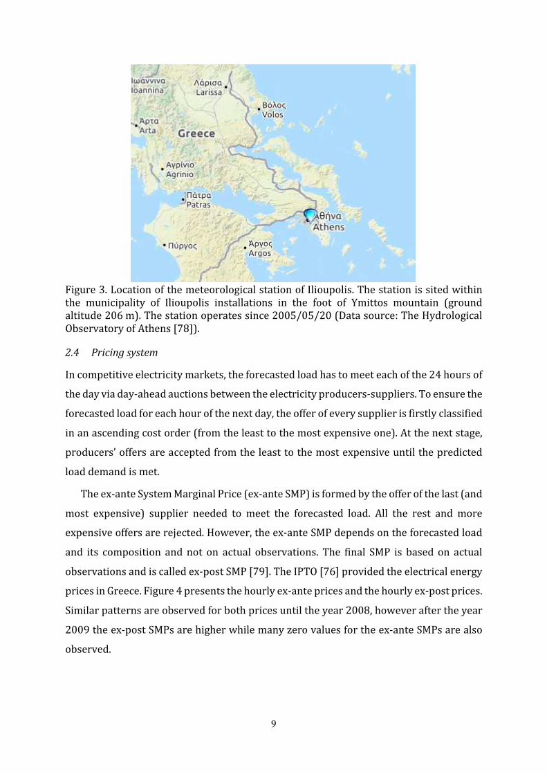
The Hydrological Observatory of Athens provided the temperature data [78]. Data from

the Ilioupolis station were used. The Ilioupolis station is located in the administrative

region of Attica (Figure 3). 35% of Greece's population resides in Attica. Furthermore, the

country's main industrial activity is concentrated in Attica. Attica’s climate is mild and the

station is located near the sea, thus the variations of temperature are less sensitive to local

weather extremes. Therefore, the station's temperature is representative of the

temperature in Greece, at least for the purpose of the analysis, despite the high

temperature variations of Greece due to its mountainous terrain. In addition, the choice

of a single station for the analysis is justified by the choice of only two stations by

Hyndman and Fan [1] in their advanced EED forecasting model.

9

Figure 3. Location of the meteorological station of Ilioupolis. The station is sited within the municipality of Ilioupolis installations in the foot of Ymittos mountain (ground altitude 206 m). The station operates since 2005/05/20 (Data source: The Hydrological Observatory of Athens [78]).

2.4 Pricing system

In competitive electricity markets, the forecasted load has to meet each of the 24 hours of

the day via day-ahead auctions between the electricity producers-suppliers. To ensure the

forecasted load for each hour of the next day, the offer of every supplier is firstly classified

in an ascending cost order (from the least to the most expensive one). At the next stage,

producers’ offers are accepted from the least to the most expensive until the predicted

load demand is met.

The ex-ante System Marginal Price (ex-ante SMP) is formed by the offer of the last (and

most expensive) supplier needed to meet the forecasted load. All the rest and more

expensive offers are rejected. However, the ex-ante SMP depends on the forecasted load

and its composition and not on actual observations. The final SMP is based on actual

observations and is called ex-post SMP [79]. The IPTO [76] provided the electrical energy

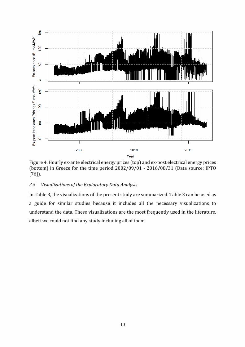
prices in Greece. Figure 4 presents the hourly ex-ante prices and the hourly ex-post prices.

Similar patterns are observed for both prices until the year 2008, however after the year

2009 the ex-post SMPs are higher while many zero values for the ex-ante SMPs are also

observed.

10

Figure 4. Hourly ex-ante electrical energy prices (top) and ex-post electrical energy prices (bottom) in Greece for the time period 2002/09/01 - 2016/08/31 (Data source: IPTO [76]).

2.5 Visualizations of the Exploratory Data Analysis

In Table 3, the visualizations of the present study are summarized. Table 3 can be used as

a guide for similar studies because it includes all the necessary visualizations to

understand the data. These visualizations are the most frequently used in the literature,

albeit we could not find any study including all of them.

11

Table 3. Figures of the present study. The examined variables and their time scale are also shown.

Description Time scale Figures Variables Time series hourly 1, 4 EED, forecasted load, prices Time series daily 18 EED, GDP, temperature Time series monthly 13 EED, forecasted load Time series annual 16 EED, GDP Histogram hourly 2, 14, 21 EED, forecasted load, prices 3D plot hourly 5 EED ACF, PACF hourly 6 EED ACF, PACF daily 6 EED ACF, PACF monthly 6 EED Extreme values hourly 8 EED Daily distribution monthly 7 EED Weekly distribution monthly 9 EED Annual distribution monthly 10, 19 EED, GDP, temperature Boxplot monthly 12 EED Scatterplot hourly 20 EED, GDP, temperature Regression scatterplot hourly 15, 22, 23 EED, forecasted load, prices Regression scatterplot annual 17, 24 EED, prices, GDP

3. VisualizationoftheEEDinthetimedomain

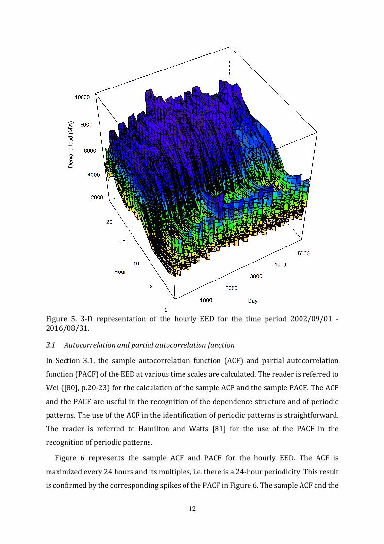
In Section 3, the EED in the time domain is visualized. In Figure 5, the data are illustrated

in three dimensions. This representation provides a better insight and additional

information about the EED variations, as proposed by Filik et al. [2]. One can observe two

constant patterns, the first in the daily distribution and the second in the annual

distribution of the EED. Furthermore, an increasing trend until day 2000 and a decreasing

trend afterwards are observed. The autocorrelations will be examined and the EED at

various time scales will be visualized in the next Sections, to better highlight the

aforementioned observations.

12

Figure 5. 3-D representation of the hourly EED for the time period 2002/09/01 - 2016/08/31.

3.1 Autocorrelation and partial autocorrelation function

In Section 3.1, the sample autocorrelation function (ACF) and partial autocorrelation

function (PACF) of the EED at various time scales are calculated. The reader is referred to

Wei ([80], p.20-23) for the calculation of the sample ACF and the sample PACF. The ACF

and the PACF are useful in the recognition of the dependence structure and of periodic

patterns. The use of the ACF in the identification of periodic patterns is straightforward.

The reader is referred to Hamilton and Watts [81] for the use of the PACF in the

recognition of periodic patterns.

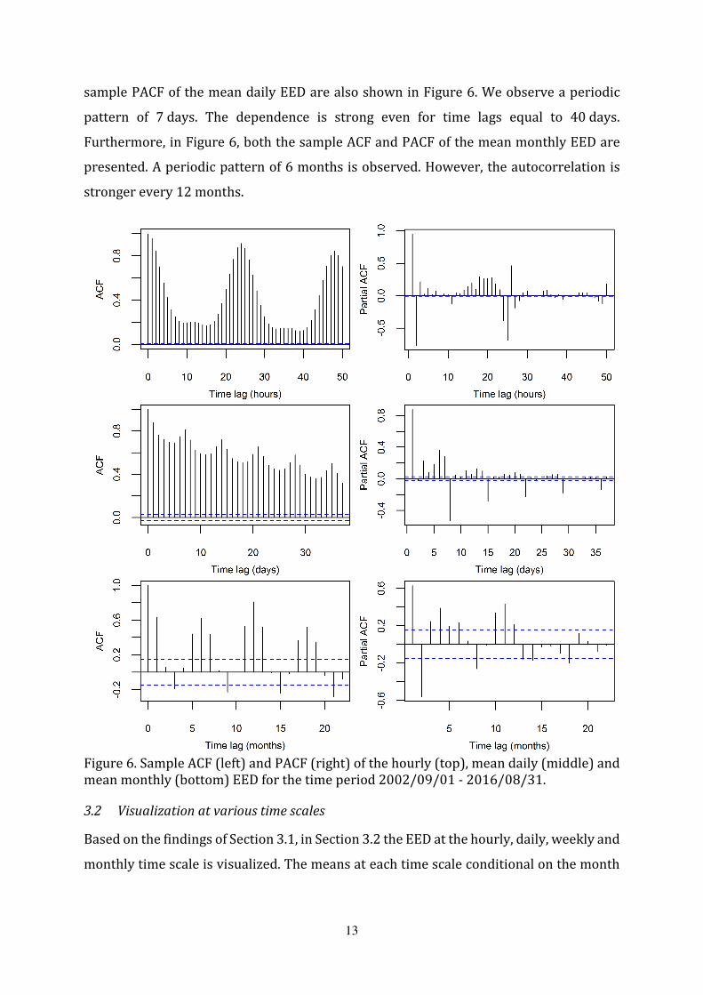
Figure 6 represents the sample ACF and PACF for the hourly EED. The ACF is

maximized every 24 hours and its multiples, i.e. there is a 24-hour periodicity. This result

is confirmed by the corresponding spikes of the PACF in Figure 6. The sample ACF and the

13

sample PACF of the mean daily EED are also shown in Figure 6. We observe a periodic

pattern of 7 days. The dependence is strong even for time lags equal to 40 days.

Furthermore, in Figure 6, both the sample ACF and PACF of the mean monthly EED are

presented. A periodic pattern of 6 months is observed. However, the autocorrelation is

stronger every 12 months.

Figure 6. Sample ACF (left) and PACF (right) of the hourly (top), mean daily (middle) and mean monthly (bottom) EED for the time period 2002/09/01 - 2016/08/31.

3.2 Visualization at various time scales

Based on the findings of Section 3.1, in Section 3.2 the EED at the hourly, daily, weekly and

monthly time scale is visualized. The means at each time scale conditional on the month

14

or the hydrological year are visualized. The results are compared with results reported in

literature about Greece.

Figure 7 presents the mean EED per hour of day, conditional on the month of the year

and the distribution of the EED during the day. While the results in Figure 7 (bottom) are

scaled, thus they seem smoother, it can furthermore be observed that the EED varies over

the year, thus a model, which considers the seasonality, is required. In the rest of Section

3.2, both the actual and the scaled EED for each time scale will be presented. In Figure 7,

it is observed that the global minimum EED values appear at approximately 3:00 to 5:00,

however another local minimum appears at approximately 16:00. Two local maxima are

also observed. The first local maximum is observed at 12:00 regardless of the month,

while the second local maximum moves from 18:00 in the winter months to 21:00 in the

summer months. The first maximum is due to the increased EED for industries, services

and household activities while the second maximum is due to household heating and

cooling. Furthermore, the latter maximum is considerably higher compared to the former

one in the winter months probably due to the increased need for heating in the night,

whereas the two maxima are approximately equal in the summer months, in which

cooling is mostly necessary in the afternoon hours. The increasing trend, observed

between 06:00 and 07:00 in the summer, moves an hour earlier during the other months.

The EED values range between these minima or maxima values during the spring and

autumn. The results are similar to those of Figure 6 in Psiloglou et al. [16], which presents

the EED distribution during the day, conditional on two months (January and July) or

summarizing the results for all months. However, the second maximum is equal or higher

than the first maximum in our study, whereas in Psiloglou et al. [16] the second maximum

is lower. It is noted here that Psiloglou et al. [16] study the EED in Athens, which may

differ compared to that of Greece.

15

Figure 7. Mean EED per hour of day (top) and distribution of the EED during the day (bottom) presented for each month of the year (bottom). The data cover the time period 2002/09/01 - 2016/08/31.

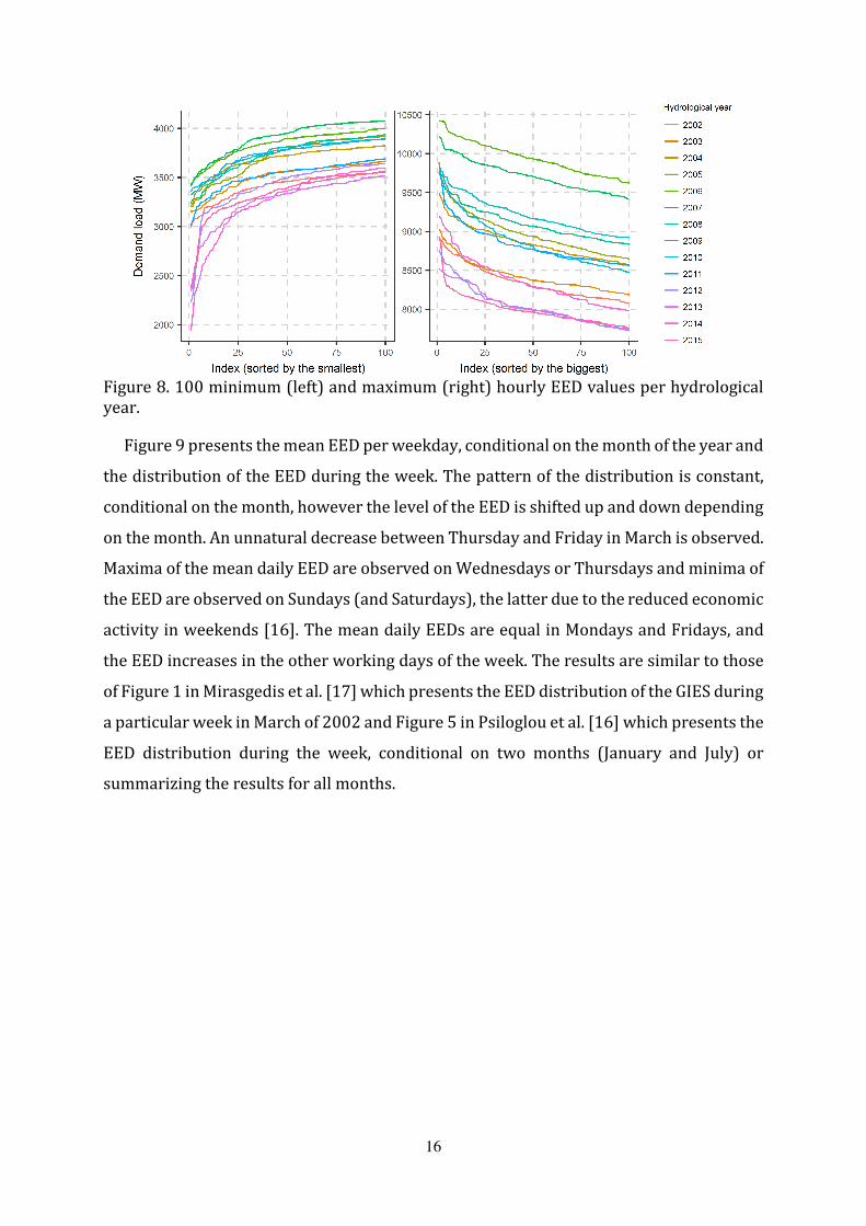
In Figure 8, the 100 minimum and maximum hourly EED values for each hydrological

year in the time period 2002 – 2015 are presented. A constant pattern of ascent in Figure

8 (left) and decay in Figure 8 (right) is observed, which is independent of the hydrological

year. However, this pattern is shifted up and down, depending on the mean annual EED.

Furthermore, in some cases the lines are intersecting, i.e. the extreme values significantly

depend on other factors, e.g. the temperature. The mean annual EED will be discussed

more thoroughly in Section 4.2.

16

Figure 8. 100 minimum (left) and maximum (right) hourly EED values per hydrological year.

Figure 9 presents the mean EED per weekday, conditional on the month of the year and

the distribution of the EED during the week. The pattern of the distribution is constant,

conditional on the month, however the level of the EED is shifted up and down depending

on the month. An unnatural decrease between Thursday and Friday in March is observed.

Maxima of the mean daily EED are observed on Wednesdays or Thursdays and minima of

the EED are observed on Sundays (and Saturdays), the latter due to the reduced economic

activity in weekends [16]. The mean daily EEDs are equal in Mondays and Fridays, and

the EED increases in the other working days of the week. The results are similar to those

of Figure 1 in Mirasgedis et al. [17] which presents the EED distribution of the GIES during

a particular week in March of 2002 and Figure 5 in Psiloglou et al. [16] which presents the

EED distribution during the week, conditional on two months (January and July) or

summarizing the results for all months.

17

Figure 9. Mean EED per weekday (top) and distribution of the EED during the week (bottom) presented for each month of the year. The data cover the time period 2002/09/01 - 2016/08/31.

Figure 10 presents the mean EED per month, conditional on the hydrological year and

the distribution of the EED during the hydrological year. Local maxima of the mean

monthly EED are observed in January and July (which is also the global maximum) and

local minima of the mean monthly EED are observed in October and April (which is also

the global minimum). The increased demand observed in the winter (December, January,

February) and the summer (June, July, August months) is associated with the increased

needs for heating and cooling respectively [16]. The EED in August is significantly lower

compared to July. This is explained by the fact that despite the mean temperatures of July

and August are similar as shown in Figure 19, August is a vacations month for industries,

which are high consumers of electrical energy [23]. The pattern is similar to that of Figure

1 in Mirasgedis et al. [17], which refers to the time period 1993-2002. However, in Figure

18

4 in Psiloglou et al. [16] a low value of the EED in August in Athens is observed. This is

probably due to the fact that August is a vacations period for most people living in Athens.

Figure 10. Mean EED per month (top) and distribution of the EED during the year (bottom) presented for each hydrological year.

In Figure 10, it is observed that the mean annual EED has reduced since the

hydrological year 2008. This is more evident in Figure 11 in which intermediate

hydrological years were omitted. This will be discussed more thoroughly in Section 4.2.

In Figure 10, it is observed that the pattern of the mean monthly EED of December and

January has changed considerably since the hydrological year 2012. This is again more

evident in Figure 11, in which some intermediate hydrological years were again omitted.

This was firstly observed by Dagoumas and Kitsios [21]. Their study refers to the

hydrological year 2012, and they attributed this change to the considerable increase of

tax on heating oil, which lead to an increase of use of electricity for heating purposes. The

19

increase of tax on heating oil was a result of the economic policy adopted by the Greek

government due to the decrease of the GDP and the economic crisis in Greece, which

started the year 2010.

Figure 11. Mean EED per month (top) and distribution of the EED during the year (bottom) presented for the hydrological years 2003, 2006, 2009, 2013.

Figure 12 presents the variance of the mean monthly EED. The highest deviations from

the mean occur in the summer months July and August. It is noted here that Figure 12 is

not comparable to Figure 3 in Psiloglou et al. [16] who study the mean daily EED.

20

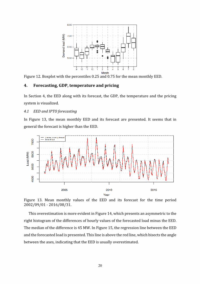
Figure 12. Boxplot with the percentiles 0.25 and 0.75 for the mean monthly EED.

4. Forecasting,GDP,temperatureandpricing

In Section 4, the EED along with its forecast, the GDP, the temperature and the pricing

system is visualized.

4.1 EED and IPTO forecasting

In Figure 13, the mean monthly EED and its forecast are presented. It seems that in

general the forecast is higher than the EED.

Figure 13. Mean monthly values of the EED and its forecast for the time period 2002/09/01 - 2016/08/31.

This overestimation is more evident in Figure 14, which presents an asymmetric to the

right histogram of the differences of hourly values of the forecasted load minus the EED.

The median of the difference is 45 MW. In Figure 15, the regression line between the EED

and the forecasted load is presented. This line is above the red line, which bisects the angle

between the axes, indicating that the EED is usually overestimated.

21

Figure 14. Histogram of hourly values of the forecasted load minus the EED for the time period 2002/09/01 - 2016/08/31.

Figure 15. Hourly EED and the forecasted load. The red line is the bisector of the angle between the two axes. The green line is the regression line between the two variables. The data cover the time period 2002/09/01 - 2016/08/31.

4.2 EED and GDP

In Figures 16 and 17, the annual GDP and the mean annual EED are presented. A linear

model for the relationship between the GDP and the EED seems reasonable, as presented

in Figure 17.

22

Figure 16. Annual GDP (top) and mean annual EED (lower) per hydrological year.

Figure 17. Annual GDP of hydrological year and mean annual EED. The continuous line is the regression line between the two variables. The coefficient of determination r2 = 0.837. The data cover the time period 2002/09/01 - 2015/08/31.

The reduction of the mean annual EED presented in Figure 16 was firstly observed by

Dagoumas and Kitsios [21] whose study ranges in the time period 1960-2012. Dagoumas

and Kitsios [21] conclude that that the decrease in the electrical energy consumption

seems to follow the economic crisis. Furthermore, the assumption of an annual increase

from 2-5% of the EED in Kalampalikas and Pilavachi [20] for the development of a model

of a power production system in Greece was not verified. Ekonomou [19] predicted an

increase in the energy consumption in Greece until the year 2015, but his prediction may

have not been verified. Regarding the Ekonomou’s [19] forecast, it is noted that he models

23

the energy consumption as a function of per resident electricity consumption. The

electrical energy consumption is the highest part of the energy consumption, thus a

decrease in EED may result in a decrease of energy consumption.

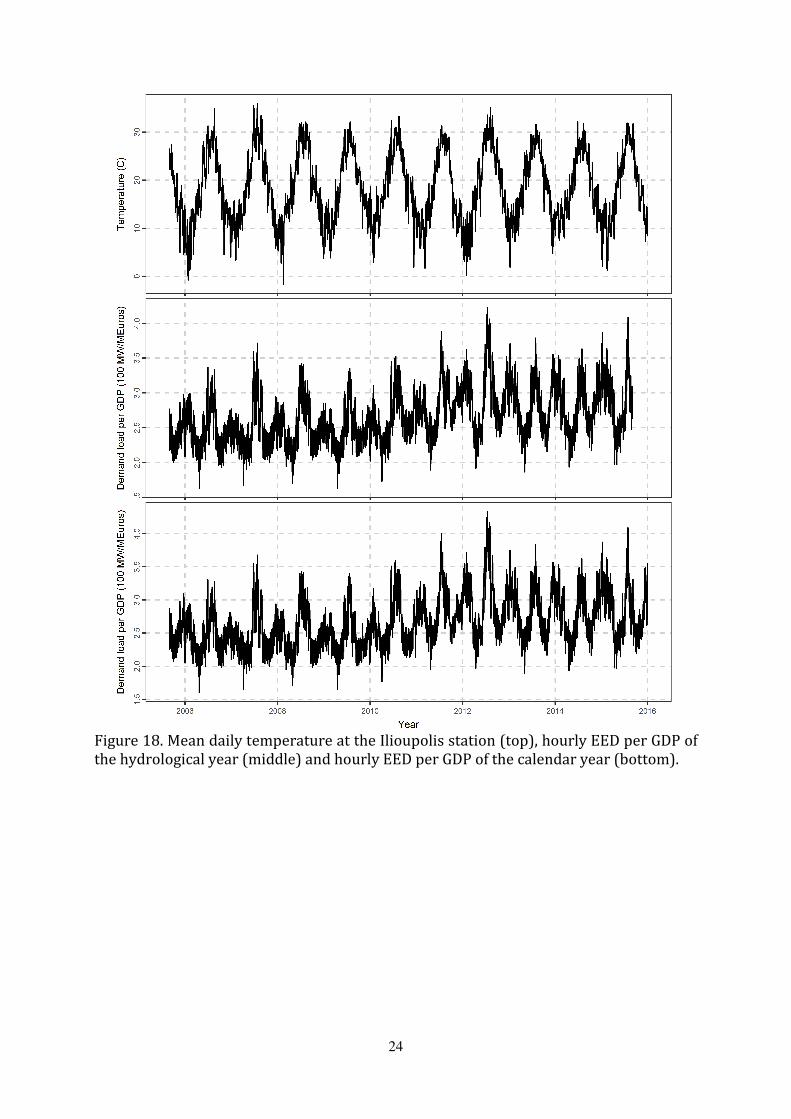
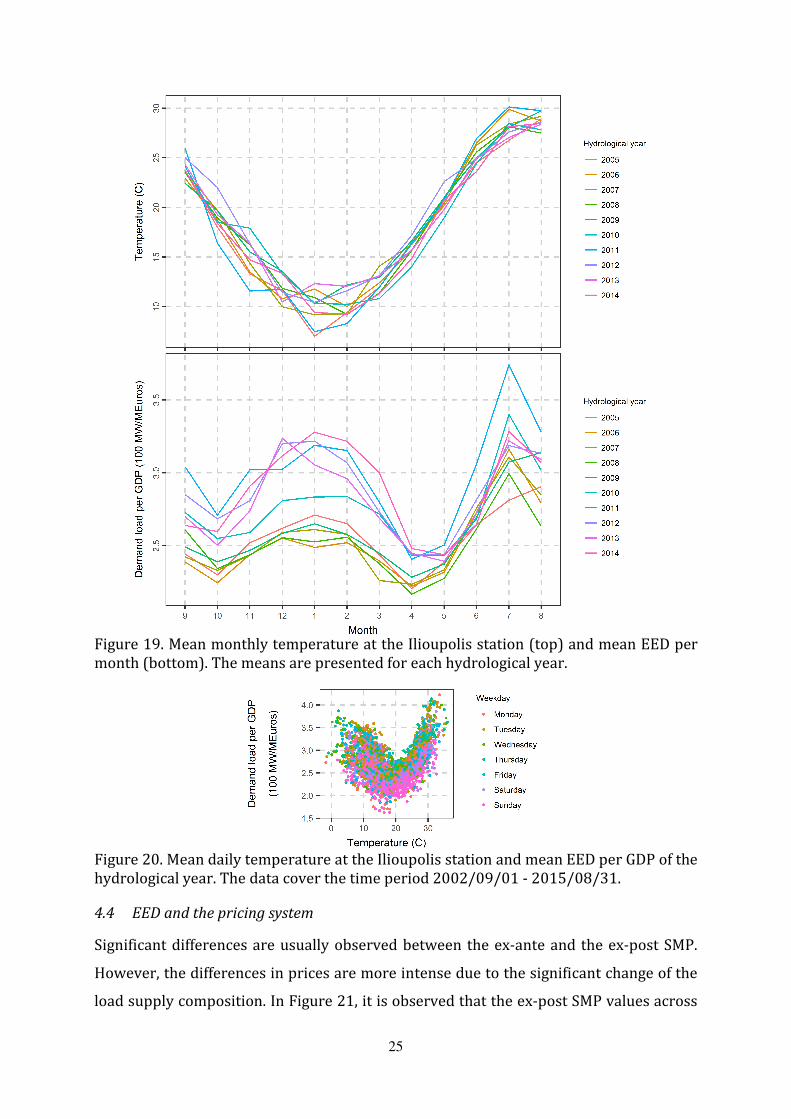
4.3 EED and temperature

Figure 18 presents the mean daily temperature at the station of Ilioupolis and the ratios

of the mean daily EED divided by the GDP of the respective year (calendar or

hydrological). A periodicity of 12 months is observed in all cases (see also Section 3.1). In

Figure 19, two local maxima of the mean monthly EED, occurring during the winter and

the summer season are observed. The winter and the summer season in Greece are

characterized by the highest and the lowest temperatures during the year respectively.

This is also confirmed in Figure 20, which indicates that a useful model for the

relationship between the mean daily temperature and the EED would be a convex curve.

The maxima of this curve appear for low or high temperatures.

Furthermore, Figure 20 is similar to Figure 8 in Psiloglou et al. [16] for Athens, Figure

2 in Mirasgedis et al. [17] for Greece and Figure 2 in Moral-Carcedo and Vicens-Otero [58]

for Spain with a similar climate to that of Greece. However, the pattern depends on the

climate, thus a different pattern in Figure 3 in Hor et al. [57] for the United Kingdom and

Figure 4 in Hyndman and Fan [1] for South Australia is observed.

24

Figure 18. Mean daily temperature at the Ilioupolis station (top), hourly EED per GDP of the hydrological year (middle) and hourly EED per GDP of the calendar year (bottom).

25

Figure 19. Mean monthly temperature at the Ilioupolis station (top) and mean EED per month (bottom). The means are presented for each hydrological year.

Figure 20. Mean daily temperature at the Ilioupolis station and mean EED per GDP of the hydrological year. The data cover the time period 2002/09/01 - 2015/08/31.

4.4 EED and the pricing system

Significant differences are usually observed between the ex-ante and the ex-post SMP.

However, the differences in prices are more intense due to the significant change of the

load supply composition. In Figure 21, it is observed that the ex-post SMP values across

26

the examined time period are much more dispersed, than the ex-ante SMP values.

Furthermore, in the two histograms it is observed that the ex-post SMP values are higher

than the ex-ante SMP values, thus the actual electrical energy price in Greece is

systematically higher than the forecasted. Additionally, as observed in Figure 4, the

deviations between the SMPs become more pronounced from the year 2009, starting to

systemically affect significantly the ex-post SMP to higher values. An event which

happened in the year 2009 was the significant introduction of renewables in the

electricity mix. Thus, the difference between the ex-ante and ex-post SMPs maybe is due

to this event, however it needs to be further investigated. The maximum SMP is

150 €/MWh as observed in Figure 21.

Figure 21. Histogram of the hourly ex-ante (left) and ex-post (right) electrical energy prices for the time period 2002/09/01 - 2016/08/31.

In Figure 22, the relationship between the EED and the ex-ante SMP, and the

relationship between the EED and the ex-post SMP are presented. It is evident from the

regression lines that the SMPs in general increase when the EED increases. In Figure 22,

a cluster of zero ex-ante SMPs for a range of hourly EEDs between 3 000-6 500 MW, and

another cluster of SMPs equal to 150 €/MWh for a range of hourly EEDs between 6 000-

8 000 MW are observed. However, in Figure 22, there is not any cluster of zero ex-post

SMPs, while the SMPs equal to 150 €/MWh range from 4 000 MW to 8 000 MW. This is an

additional indication that the ex-post SMP is systematically higher than the ex-ante SMP.

On the other hand, a linear relationship would not be a reasonable model for the relation

between the SMP and the demand load, as it is also suggested by the low coefficient of

determination r2.

27

Figure 22. Hourly EED and ex-ante (left), ex-post (right) electrical energy prices for the time period 2002/09/01 - 2016/08/31. The red line is the regression line between the two variables.

Although it would be expected that high SMPs correspond to high EEDs, Figure 22

reveals a different behaviour, i.e. extremely high prices can be observed frequently even

at relatively low or medium EEDs (4 000-6 000 MW). A possible explanation for this

behaviour is that it is due to the peculiarities of the Greek electricity market with respect

to the renewables. Furthermore, it is noted that the renewables’ share in the electricity

mix is higher for low or medium EEDs [82].

Figure 23 clarifies the indications of Figure 22. In Figure 21, it is observed that the main

mass of SMPs is concentrated in values less than 115 €/MWh. The regression line in

Figure 23 signifies that the ex-post SMP is systematically higher than the corresponding

ex-ante SMP in the aforementioned region. The ex-ante SMP is higher than the

corresponding expected ex-post SMP for ex-ante SMPs higher than approximately

115 €/MWh.

28

Figure 23. Hourly ex-ante and ex-post electrical energy prices for the time period 2002/09/01 - 2016/08/31. The red line bisects the angle between the two axes. The green line is the regression line between the two variables.

In Figure 24, it is observed that the mean annual demand load increases slightly with

the increase of the mean annual SMP price. Pearson’s r is low, indicating that no linear

relationship exists between the two variables, therefore the influence of the price should

be examined using additional information from other variables.

Figure 24. Mean annual EED and mean annual ex-post electrical energy price of hydrological year for the time period 2002/09/01 - 2016/08/31. The continuous line is the regression line between the two variables. The coefficient of determination r2 = 0.04.

5. Discussionofresults

To summarize the findings of the study, three types of periodicities, i.e. periodic patterns

of 24 hours, 7 days and 12 months were observed. The distribution of the EED in the daily,

weekly and annual time scale, along with the minimum and maximum values were

visualized.

29

A linear model for the relationship between energy demand and GDP seems

reasonable, i.e. the increase of the GDP results in increasing EED (or vice versa). The

relationship between the mean daily temperature and the EED could be modelled with a

convex curve. The maxima of this curve appear for low or high temperatures. This result

is consistent with the result for the mean monthly EED values. Some side results of our

analysis is that the IPTO forecast is usually higher than the observed EED, however, this

difference is acceptable. Regarding the difference between the ex-ante and ex-post SMP

values, it increases in favour of the ex-post SMP values since the year 2009.

Besides the expected patterns found, some details revealed by the EDA could

considerably improve the building of forecasting models, thus highlighting its importance.

One important result is that the price of oil may change the distribution of the EED during

the year in a non-linear way. Thus, the price of fossil fuels should be considered in the

modelling of the EED. Indeed, changes of variables such as the GDP, prices of heating oil

etc., assumed to influence the EED in big time scales may also, influence the distribution

of the EED during the year and consequently the maximum and minimum observed values

and the mean weekly EEDs. Particularly, different economic variables may interact, e.g.

the decrease of the GDP resulted in the increase of the price of fossil fuels as was explained

in Section 3.2. This is important because time series models cannot model such

deterministic changes. Therefore, the interaction of socio-economic factors and weather

and climatic variables should always be considered, as well as their non-linear effects on

the EED.

The varying levels of the variation of the EED from month to month should also been

considered in the modelling, because the usual time series models, e.g. ARMA, ARIMA etc.,

are applied under the assumption of a constant standard deviation during the year, which

is invalid in the present case.

6. Conclusions

Regarding the contributions of the present study, it is noticed that we found only one

similar study in Greece, which investigated the electrical energy demand in Athens (the

capital city) and used data from the time period 1997-2001, whereas in the present study

a longer time period (2002-2015) is covered and more recent data are used. Furthermore,

another study that presents in such detail the electrical energy demand in the time

30

domain and its relationship to a big number of weather-, climate-related and socio-

economic variables was not found.

The results of the present study confirm and summarize the conclusions of previous

relevant studies in Greece with the exception of studies that forecasted the mean annual

electrical energy demand. These studies failed to forecast the gross domestic product

decrease, observed in recent years, and subsequently failed to forecast the electrical

energy demand decrease. In addition, some unexpected behaviours were noticed, related

to the change in the annual distribution of the electrical energy demand due to the

increase in the oil prices and a non-stationarity regarding the variation of the mean

monthly electrical energy demand, which if not modelled properly could result in dubious

forecasts. These results highlight the importance of performing a detailed exploratory

data analysis before modelling the electrical energy demand. Regarding the management

of the GIES, its efficient operation in the short-term is noted, however there is still place

for improvement.

On the other hand, special attention should be given to the short- and long-term

planning due to the uncertainty in the forecasting of socio-economic variables, the

interaction between the socio-economic variables and the modelling of the relationship

between socio-economic variables and the electrical energy demand in small time scales.

Indeed the socio-economic variables are subject to unexpected changes due to the

unpredictability of the human behaviour therefore modelling of socio-economic variables

is important and consequently an interdisciplinary approach is necessary.

The existence of software for electrical energy demand forecasting is noted, however

its general use is not recommended, because the models are location-specific, hence not

general. The exploratory data analysis of the electrical energy demand is necessary to

investigate the usefulness of a model or a software in modelling the electrical energy

demand, before using it. The framework introduced in the present study in which the

electrical energy demand, the gross domestic product, the electricity price and the

temperature were visualized in various time scales to highlight their interactions can

serve as a blueprint for performing an exploratory data analysis.

We think that the results of our study are useful for building a model for short-,

medium- and long-term electrical energy demand forecasting. This model could be

applied in formulating a management policy for the daily operation, the maintenance

31

planning and the expansion of the GIES. This model could also be used for the simulation

of the GIES under various scenarios, regarding the installation of new energy systems,

improving the planning strategy. It is also noted that the building of a model for the

electrical energy demand in Greece is out of the scope of this study. In this manuscript,

the code and the data are also provided, so that the reader can reproduce the results and

create new work based on the present research.

Acknowledgement: The authors wish to thank three anonymous reviewers for their

constructive comments, which helped to improve the quality of the manuscript

significantly. They also thank Dr. Nikolaos Kouveliotis for the constructive discussion

about the Greek Electric System.

Funding information: This research has been partly funded by the Greek General

Secretariat for Research and Technology through the research project “Combined

REnewable Systems for Sustainable Energy DevelOpment” (CRESSENDO project, grant

number 5145).

References

[1] Hyndman RJ, Fan S. Density Forecasting for Long-Term Peak Electricity Demand. IEEE T Power Syst 2010;25(2):1142–1153. http://dx.doi.org/10.1109/TPWRS.2009.2036017.

[2] Filik ÜB, Gerek ÖN, Kurban M. A novel modeling approach for hourly forecasting of long-term electric energy demand. Energ Convers Manage 2011;52(1):199–211. http://dx.doi.org/10.1016/j.enconman.2010.06.059.

[3] Hong T, Fan S. Probabilistic electric load forecasting: A tutorial review. Int J Forecasting 2016;32(3):914–938. http://dx.doi.org/10.1016/j.ijforecast.2015.11.011.

[4] Zachariadis T, Pashourtidou N. An empirical analysis of electricity consumption in Cyprus. Energ Econ 2007;29(2):183–198. http://dx.doi.org/10.1016/j.eneco.2006.05.002.

[5] Payne JE. A survey of the electricity consumption-growth literature. Appl Energy 2010;87(3):723–731. doi:http://dx.doi.org/10.1016/j.apenergy.2009.06.034.

[6] Polemis ML, Dagoumas AS. The electricity consumption and economic growth nexus: Evidence from Greece. Energy Policy 2013;62:798–808. http://dx.doi.org/10.1016/j.enpol.2013.06.086.

[7] Kıran MS, Özceylan E, Gündüz M, Paksoy T. A novel hybrid approach based on Particle Swarm Optimization and Ant Colony Algorithm to forecast energy demand of Turkey. Energ Convers Manage 2012;53(1):75–83. http://dx.doi.org/10.1016/j.enconman.2011.08.004.

[8] Farzan F, Jafari MA, Gong J, Farzan F, Stryker A. A multi-scale adaptive model of residential energy demand. Appl Energy 2015;150:258–273. http://dx.doi.org/10.1016/j.apenergy.2015.04.008.

[9] Tukey JW. Exploratory data analysis. Pearson Addison Wesley; 1977.

32

[10] Behrens JT, Yu CH. Exploratory Data Analysis. In: Schinka JA, Velicer WF, editors. Handbook of Psychology, Volume 2: John Wiley & Sons, Inc; 2003, p. 33–64. http://dx.doi.org/10.1002/0471264385.wei0202.

[11] Behrens JT. Principles and procedures of exploratory data analysis. Psychol Methods 1997;2(2):131–160. http://dx.doi.org/10.1037/1082-989X.2.2.131.

[12] Chatfield C. Exploratory data analysis. Eur J Oper Res 1986;23(1):5–13. http://dx.doi.org/10.1016/0377-2217(86)90209-2.

[13] Box GEP. Robustness in the Strategy of Scientific Model Building. In: Launer RL, Wilkinson GN, editors. Robustness in Statistics: Academic Press; 1979, p. 201–236.

[14] Kalampalikas NG, Pilavachi PA. A model for the development of a power production system in Greece, Part II: Where RES meet EU targets. Energy Policy 2010b;38(11):6514–6528. http://dx.doi.org/10.1016/j.enpol.2010.05.037.

[15] Andrianesis P, Biskas P, Liberopoulos G. An overview of Greece’s wholesale electricity market with emphasis on ancillary services. Electr Pow Syst Res 2011;81(8):1631–1642. http://dx.doi.org/10.1016/j.epsr.2011.04.005.

[16] Psiloglou BE, Giannakopoulos C, Majithia S, Petrakis M. Factors affecting electricity demand in Athens, Greece and London, UK: A comparative assessment. Energy 2009;34(11):1855–1863. http://dx.doi.org/10.1016/j.energy.2009.07.033.

[17] Mirasgedis S, Sarafidis Y, Georgopoulou E, Lalas DP, Moschovits M, Karagiannis F, Papakonstantinou D. Models for mid-term electricity demand forecasting incorporating weather influences. Energy 2006;31(2–3):208–227. http://dx.doi.org/10.1016/j.energy.2005.02.016.

[18] Pappas SS, Ekonomou L, Karampelas P, Karamousantas DC, Katsikas SK, Chatzarakis GE, Skafidas PD. Electricity demand load forecasting of the Hellenic power system using an ARMA model. Electr Pow Syst Res 2010;80(3):256–264. http://dx.doi.org/10.1016/j.epsr.2009.09.006.

[19] Ekonomou L. Greek long-term energy consumption prediction using artificial neural networks. Energy 2010;35(2):512–517. http://dx.doi.org/10.1016/j.energy.2009.10.018.

[20] Kalampalikas NG, Pilavachi PA. A model for the development of a power production system in Greece, Part I: Where RES do not meet EU targets. Energy Policy 2010a;38(11):6499–6513. http://dx.doi.org/10.1016/j.enpol.2010.05.038.

[21] Dagoumas A, Kitsios F. Assessing the impact of the economic crisis on energy poverty in Greece. Sustain Cities Soc 2014;13:267–278. http://dx.doi.org/10.1016/j.scs.2014.02.004.

[22] Tyralis H, Mamassis N, Photis YN. Spatial Analysis of Electrical Energy Demand Patterns in Greece: Application of a GIS-based Methodological Framework. Energy Procedia 2016;97:262–269. http://dx.doi.org/10.1016/j.egypro.2016.10.071.

[23] Tyralis H, Mamassis N, Photis YN. Spatial analysis of the electrical energy demand in Greece. Energy Policy 2017;102:340–352. http://dx.doi.org/10.1016/j.enpol.2016.12.033.

[24] Tsani SZ. Energy consumption and economic growth: A causality analysis for Greece. Energ Econ 2010;32(3):582–590. http://dx.doi.org/10.1016/j.eneco.2009.09.007.

[25] Fuinhas JA, Marques AC. Energy consumption and economic growth nexus in Portugal, Italy, Greece, Spain and Turkey: An ARDL bounds test approach (1965–2009). Energ Econ 2012;34(2):511–517. http://dx.doi.org/10.1016/j.eneco.2011.10.003.

33

[26] Dergiades T, Martinopoulos G, Tsoulfidis L. Energy consumption and economic growth: Parametric and non-parametric causality testing for the case of Greece. Energ Econ 2013;36:686–697. http://dx.doi.org/10.1016/j.eneco.2012.11.017.

[27] Marques AC, Fuinhas JA, Menegaki AN. Interactions between electricity generation sources and economic activity in Greece: A VECM approach. Appl Energy 2014;132:34–46. http://dx.doi.org/10.1016/j.apenergy.2014.06.073.

[28] Slini T, Giama E, Papadopoulos AM. The impact of economic recession on domestic energy consumption. Int J Sustain Energy 2015;34(3–4):259–270. http://dx.doi.org/10.1080/14786451.2014.882335.

[29] Azam M, Khan AQ, Zafeiriou E, Arabatzis G. Socio-economic determinants of energy consumption: An empirical survey for Greece. Renew Sustain Energy Rev 2016;57: 1556–1567. http://dx.doi.org/10.1016/j.rser.2015.12.082.

[30] Katsoulakos NM, Kaliampakos DC. What is the impact of altitude on energy demand? A step towards developing specialized energy policy for mountainous areas. Energy Policy 2014;71:130–138. http://dx.doi.org/10.1016/j.enpol.2014.04.003.

[31] Panagiotopoulos G, Katsoulakos NM. Specification of the socioeconomic dimensions of energy demand and consumption in Greece, using Geographical Information Systems, http://www.researchgate.net/profile/Nikolas_Katsoulakos/publication/267334835_Specification_of_the_socioeconomic_dimensions_of_energy_demand_and_consumption_in_Greece_using_Geographical_Information_Systems/links/544cbb530cf24b5d6c40c70d.pdf; 2014 [accessed 22.05.17]

[32] Katsoulakos NM, Kaliampakos DC. Mountainous areas and decentralized energy planning: Insights from Greece. Energy Policy 2016;91:174–188. http://dx.doi.org/10.1016/j.enpol.2016.01.007.

[33] Halkos GE, Tzeremes NG. Analyzing the Greek renewable energy sector: A Data Envelopment Analysis approach. Renew Sustain Energy Rev 2012;16(5):2884–2893. http://dx.doi.org/10.1016/j.rser.2012.02.003.

[34] Katsaprakakis DA, Christakis DG. The exploitation of electricity production projects from Renewable Energy Sources for the social and economic development of remote communities. The case of Greece: An example to avoid. Renew Sustain Energy Rev 2016;54:341–349. http://dx.doi.org/10.1016/j.rser.2015.10.029.

[35] Papadelis S, Stavrakas V, Flamos A. What Do Capacity Deployment Rates Tell Us about the Efficiency of Electricity Generation from Renewable Energy Sources Support Measures in Greece?. Energies 2016;9(1):38. http://dx.doi.org/10.3390/en9010038.

[36] Hondroyiannis G. Estimating residential demand for electricity in Greece. Energ Econ 2004;26(3):319–334. http://dx.doi.org/10.1016/j.eneco.2004.04.001.

[37] Rapanos VT, Polemis ML (2006) The structure of residential energy demand in Greece. Energy Policy 34(17):3137–3143. http://dx.doi.org/10.1016/j.enpol.2005.05.017.

[38] Koroneos CJ, Nanaki EA, Xydis GA. Exergy analysis of the energy use in Greece. Energy Policy 2011;39(5):2475–2481. http://dx.doi.org/10.1016/j.enpol.2011.02.012.

[39] Doukas H, Karakosta C, Flamos A, Psarras J. Foresight for Energy Policy: Techniques and Methods Employed in Greece. Energ Source Part B 2014;9(2):109–119. http://dx.doi.org/10.1080/15567241003735217.

34

[40] Zachariadis T, Hadjinicolaou P. The effect of climate change on electricity needs – A case study from Mediterranean Europe. Energy 2014;76:899–910. http://dx.doi.org/10.1016/j.energy.2014.09.001.

[41] Amina M, Kodogiannis VS, Petrounias I, Tomtsis D. A hybrid intelligent approach for the prediction of electricity consumption. Int J Elec Power 2012;43(1):99–108. http://dx.doi.org/10.1016/j.ijepes.2012.05.027.

[42] Soytas U, Sari R. Energy consumption and GDP: causality relationship in G-7 countries and emerging markets. Energ Econ 2003;25(1):33–37. http://dx.doi.org/10.1016/S0140-9883(02)00009-9.

[43] Mozumder P, Marathe A. Causality relationship between electricity consumption and GDP in Bangladesh. Energy Policy 2007;35(1):395–402. http://dx.doi.org/10.1016/j.enpol.2005.11.033.

[44] Ouédraogo IM. Electricity consumption and economic growth in Burkina Faso: A cointegration analysis. Energ Econ 2010;32(3):524–531. http://dx.doi.org/10.1016/j.eneco.2009.08.011.

[45] López M, Valero S, Senabre C, Aparicio J, Gabaldon A. Application of SOM neural networks to short-term load forecasting: The Spanish electricity market case study. Electr Pow Syst Res 2012;91:18–27. http://dx.doi.org/10.1016/j.epsr.2012.04.009.

[46] Hainoun A, Seif-Eldin MK, Almoustafa S. Analysis of the Syrian long-term energy and electricity demand projection using the end-use methodology. Energy Policy 2006;34(14):1958–1970. http://dx.doi.org/10.1016/j.enpol.2004.12.024.

[47] Shan B, Xu M, Zhu F, Zhang C. China's Energy Demand Scenario Analysis in 2030. Energy Procedia 2012;14:1292–1298. http://dx.doi.org/10.1016/j.egypro.2011.12.1091.

[48] Gürbüz F, Öztürk C, Pardalos P. Prediction of electricity energy consumption of Turkey via artificial bee colony: a case study. Energ Syst 2013;4(3):289–300. http://dx.doi.org/10.1007/s12667-013-0079-z.

[49] Morales-Acevedo A. Forecasting Future Energy Demand: Electrical Energy in Mexico as an Example Case. Energy Procedia 2014;57:782–790. http://dx.doi.org/10.1016/j.egypro.2014.10.286.

[50] Ferruzzi G, Cervone G, Monache L Delle, Graditi G, Jacobone F. Optimal bidding in a Day-Ahead energy market for Micro Grid under uncertainty in renewable energy production. Energy 2016;106(1):194–202. http://dx.doi.org/10.1016/j.energy.2016.02.166.

[51] Graditi G, Ferlito S, Adinolfi G, Tina GM, Ventura C. Energy yield estimation of thin-film photovoltaic plants by using physical approach and artificial neural networks. Sol Energy 2016;130:232–243. http://dx.doi.org/10.1016/j.solener.2016.02.022.

[52] Akinlo AE. Electricity consumption and economic growth in Nigeria: Evidence from cointegration and co-feature analysis. J Policy Model 2009;31(5):681–693. http://dx.doi.org/10.1016/j.jpolmod.2009.03.004.

[53] Kumar U, Jain VK. Time series models (Grey-Markov, Grey Model with rolling mechanism and singular spectrum analysis) to forecast energy consumption in India. Energy 2010;35(4):1709–1716. http://dx.doi.org/10.1016/j.energy.2009.12.021.

[54] Yu S, Wei YM, Wang K. A PSO–GA optimal model to estimate primary energy demand of China. Energy Policy 2012;42:329–340. http://dx.doi.org/10.1016/j.enpol.2011.11.090.

35

[55] Yu S, Zhu K, Zhang X. Energy demand projection of China using a path-coefficient analysis and PSO–GA approach. Energ Convers Manage 2012;53(1):142–153. http://dx.doi.org/10.1016/j.enconman.2011.08.015.

[56] Pardo A, Meneu V, Valor E. Temperature and seasonality influences on Spanish electricity load. Energ Econ 2002;24(1):55–70. http://dx.doi.org/10.1016/S0140-9883(01)00082-2.

[57] Hor CL, Watson SJ, Majithia S. Analyzing the impact of weather variables on monthly electricity demand. IEEE T Power Syst 2005;20(4):2078–2085. http://dx.doi.org/10.1109/TPWRS.2005.857397.

[58] Moral-Carcedo J, Vicens-Otero J. Modelling the non-linear response of Spanish electricity demand to temperature variations. Energ Econ 2005;27(3):477–494. http://dx.doi.org/10.1016/j.eneco.2005.01.003.

[59] De Cian E, Lanzi E, Roson R. Seasonal temperature variations and energy demand. A panel cointegration analysis for climate change impact assessment. Climatic Change 2013;116(3-4):805–825. http://dx.doi.org/10.1007/s10584-012-0514-5.

[60] Gam I, Rejeb JB. Electricity demand in Tunisia. Energy Policy 2012;45:714–720. http://dx.doi.org/10.1016/j.enpol.2012.03.025.

[61] Thornton HE, Hoskins BJ, Scaife AA. The role of temperature in the variability and extremes of electricity and gas demand in Great Britain. Environ Res Lett 2016;11(114015). http://dx.doi.org/10.1088/1748-9326/11/11/114015.

[62] Dimitropoulos J, Hunt LC, Judge G. Estimating underlying energy demand trends using UK annual data. Appl Econ Lett 2005;12(4):239–244. http://dx.doi.org/10.1080/1350485052000337789.

[63] Dilaver Z, Hunt LC. Industrial electricity demand for Turkey: A structural time series analysis. Energ Econ 2011;33(3):426–436. http://dx.doi.org/10.1016/j.eneco.2010.10.001.

[64] Richardson I, Thomson M, Infield D, Clifford C. Domestic electricity use: A high-resolution energy demand model. Energ Buildings 2010;42(10):1878–1887. http://dx.doi.org/10.1016/j.enbuild.2010.05.023.

[65] Widén J, Wäckelgård E. A high-resolution stochastic model of domestic activity patterns and electricity demand. Appl Energy 2010;87(6):1880–1892. http://dx.doi.org/10.1016/j.apenergy.2009.11.006.

[66] Ferruzzi G, Graditi G, Rossi F, Russo A. Optimal Operation of a Residential Microgrid: The Role of Demand Side Management. Intell Ind Syst 2015;1(1):61–82. http://dx.doi.org/10.1007/s40903-015-0012-y.

[67] Jebaraj S, Iniyan S. A review of energy models. Renew Sustain Energy Rev 2006;10(4):281–311. http://dx.doi.org/10.1016/j.rser.2004.09.004.

[68] Suganthi L, Samuel AA. Energy models for demand forecasting—A review. Renew Sustain Energy Rev 2012;16(2):1223–1240. http://dx.doi.org/10.1016/j.rser.2011.08.014.

[69] Ghalehkhondabi I, Ardjmand E, Weckman GR, Young II WA. An overview of energy demand forecasting methods published in 2005–2015. Energ Syst 2017;8(2):411–447. http://dx.doi.org/10.1007/s12667-016-0203-y.

[70] Aggarwal SK, Saini LM, Kumar A. Electricity price forecasting in deregulated markets: A review and evaluation. Int J Elec Power 2009;31(1):13–22. http://dx.doi.org/10.1016/j.ijepes.2008.09.003.

[71] Dudek G. Multilayer perceptron for GEFCom2014 probabilistic electricity price forecasting. Int J Forecasting 2016;32(3):1057–1060. http://dx.doi.org/10.1016/j.ijforecast.2015.11.009.

36

[72] Hippert HS, Pedreira CE. Estimating temperature profiles for short-term load forecasting: neural networks compared to linear models. IEE P-Gener Transm D 2004;151(4):543–547. http://dx.doi.org/10.1049/ip-gtd:20040491.

[73] Narayan A, Hipel KW, Ponnambalam K, Paul S. Neuro-fuzzy inference system (ASuPFuNIS) model for intervention time series prediction of electricity prices. IEEE Sys Man Cybern 2011;2121–2126. http://dx.doi.org/10.1109/ICSMC.2011.6083985.

[74] Vaghefi A, Jafari MA, Bisse E, Lu Y, Brouwer J. Modeling and forecasting of cooling and electricity load demand. Appl Energy 2014;136:186–196. http://dx.doi.org/10.1016/j.apenergy.2014.09.004.

[75] Tyralis H, Karakatsanis G, Tzouka K, Mamassis N. Data and code for the exploratory data analysis of the electrical energy demand in the time domain in Greece. Data in Brief 2017; (in review).

[76] Independent Power Transmission Operator. Electricity/Power Market Participation, Market Data, http://www.admie.gr/leitoyrgia-dedomena/leitoyrgia-agoras-ilektrikis-energeias/anafores-dimosieyseis-agoras/; 2017 [accessed 06.01.17].

[77] The World Bank. World Development Indicators, http://data.worldbank.org/country/Greece; 2016 [accessed 14.08.16].

[78] The Hydrological Observatory of Athens. List of Stations, http://hoa.ntua.gr/stations/l/?&owner=3; 2017 [accessed 06.01.17].

[79] Independent Power Transmission Operator. Manual of Market Clearance (version 3, in Greek), http://www.admie.gr/fileadmin/groups/EDRETH/Manuals/Egcheiridio_Ekkatharisis_Agoras_v3.0.pdf; 2012a [accessed 22.05.17].

[80] Wei WWS. Time Series Analysis, Univariate and Multivariate Methods. 2nd ed. Pearson Addison Wesley; 2006.

[81] Hamilton DC, Watts DG. Interpreting partial autocorrelation functions of seasonal time series models. Biometrika 1978;65(1):135–140. http://dx.doi.org/10.2307/2335288.

[82] Independent Power Transmission Operator. Manual of Power Sufficiency Mechanism (version 3, in Greek), http://www.admie.gr/uploads/media/MANUAL_CAM_v3_TC.pdf; 2012b [accessed 22.05.17].