Embed Size (px)
Citation preview
CERDI, Etudes et Documents, E 2002.27
Document de travail de la série
Etudes et Documents
E 2002.27
Explaining the Negative Coefficient Associated with Human Capital
in Augmented Solow Growth Regressions∗
Jean-Louis ARCAND, Béatrice D'HOMBRES
This draft: September 2002 - 47 p. Comments Welcome
CERDI-CNRS, Université d'Auvergne 65, boulevard François Mitterrand - 63000 Clermont Ferrand -France tel : +33-4-73177400 - fax : +33-4-73177428 email: [email protected] - [email protected] http: www.cerdi.org
∗
We thank Jerry Hausman for his kind help concerning IV estimation in general and our new GMM estimator in particular. The usual disclaimer, however, applies.
CERDI, Etudes et Documents, E 2002.27
2
Abstract In this paper we consider different explanations for why the coefficient associated with human capital is often negative in growth regressions once country-specific effects are controlled for whereas the coefficient in question is strongly positive in cross-sectional or panel results based on the pooling estimator. In turn, we explore: (i) additional sources of unobserved heterogeneity stemming from country-specific rates of labor-augmenting technological change, (ii) measurement error in the human capital series being used, and (iii) the lack of variability in the human capital series once the usual covariance transformations are implemented. Remaining unobserved country-specific heterogeneity and measurement error alone are shown to be inadequate explanations. The lack of variability in the human capital series is tackled using a new GMM-based estimator that combines the Hausman-Taylor (1981) approach, in which the impact of time-invariant covariates can be identified through use of covariance transformations of the variables themselves as instruments, with the orthogonality conditions of the Arellano-Bond (1991) estimator. Keywords: Economic growth, human capital, measurement error, panel
estimation.
Résumé
Pourquoi le coefficient associé au capital humain dans un modèle de Solow Augmenté est-il négatif ?
Cet article a pour objet d’étudier les différentes explications susceptibles de conduire dans une estimation de croissance à un coefficient associé à l’éducation tantôt négatif en effet fixe et tantôt positif en pooling. Ainsi, nous étudions successivement les biais liés (i) à la non prise en compte de l’hétérogénéité non observable dans le taux d’accumulation du progrès technologique, (ii) à l’erreur de mesure associée à la variable de capital humain traditionnellement utilisée, (iii) au manque de variabilité de la variable de capital humain une fois effectuées les transformations en effets fixes ou en différence première. Les biais causés par la non prise en compte des effets simultanés de l’erreur de mesure et du manque de variabilité sont contrecarrés par l’utilisation d’un nouvel estimateur de variables instrumentales qui combine à la fois l’approche de Hausman-Taylor (1981) et les conditions d’orthogonalités de l’estimateur de Arellano-Bond (1991). Mots clés : croissance économique, capital humain, erreur de mesure, estimation
en panel.
JEL: E13, C230, O400, O150.
CERDI, Etudes et Documents, E 2002.27
3
1. INTRODUCTION
Since the seminal empirical contributions by Mankiw, Romer and Weil (1992, henceforth
MRW) and Benhabib and Spiegel (1994), there has been a fundamental tension between
cross-sectional and panel data results concerning the impact of education on the process of
economic growth. Results based on cross-sectional data over 25 year time spans (or longer),
such as those presented by MRW, indicate a strong positive effect of various measures of
human capital on economic growth. In contrast, once country-specific fixed effects are
controlled for, as in Benhabib and Spiegel (1994) or Islam (1995), the coefficient associated
with human capital becomes either statistically indistinguishable from zero or negative and
statistically significant at the usual levels of confidence.1 Table 1 summarizes a number of
recent empirical findings that follow this pattern, and underscores their worrisome nature.
Given the high proportion of government expenditures devoted to education, the question that
immediately arises, as it was cogently put by Pritchett (1997) is : Where has all the education
gone ?2
The reason for including human capital in an empirical implementation of the Solow growth
model –the point of departure for the contribution of MRW– was to reduce the point estimate
of the coefficient associated with physical capital, held to be much too high in light of the
mean value of labor’s share in GDP across countries and across time periods.3 In a restricted
Solow growth regression estimated over the period 1960-1985, the point estimate of α , the
share of capital in GDP, was found by MRW to be equal to 0.6.4 Including human capital in
the specification brought it down to the much more acceptable level of 0.31, with education’s
1 As Benhabib and Spiegel (1994, p. 154) put it, “the coefficient for human capital is insignificant and enters with the wrong sign…. whether we use the Kyriacou, Barro-Lee, or literacy data sets as proxies for the stock of human capital,” while Islam (1995, p. 1153) states that “the coefficient on the human capital variable now appears…with the wrong sign….Whenever researchers have attempted to incorporate the temporal dimension of human capital variables into growth regressions, outcomes of either statistical insignificance or negative sign have surfaced.” 2 Pritchett uses one human capital stock and instruments using another in his specification. This method, known as the "indicator variable" approach, is well described in Wooldridge (2002). 3 The issue of the “appropriate” value of capital's share has been considered by a number of authors. Hamilton and Monteagudo (1998) consider a vintage capital model that explains the lack of correspondence between the coefficient on capital in the estimation and the share of capital in GDP (see their references on p. 506). Gollin (2001) revises the estimates of labor’s share of income (usually based on employee compensation) using data on self-employment and small enterprises, and shows that conventional estimates are likely to be severely biased for poor countries. 4 MRW, 1992, Table I, p. 414; Islam, 1995, obtains 0.83, Table 1, p. 1141.

CERDI, Etudes et Documents, E 2002.27
4
share coming in at 0.28.5 As such, the augmented Solow specification on cross-sectional data
can be said to have accomplished its mission.
With the increasing availability of internationally comparable panel data, however, it became
difficult to justify estimating growth regressions on cross sections, given that the data, as well
as the appropriate econometric techniques, allowed one to control for country-specific
unobserved heterogeneity. As is well-known, failure to control for individual effects tends to
bias point estimates upwards, when the individual effects in question are positively correlated
with the variable whose marginal impact one is trying to estimate. As such, panel estimation
through some sort of covariance transformation (such as fixed effects) provides one with an
additional tool that can, a priori, bring down the point estimate of the coefficient associated
with physical capital, and provide more robust estimates of the marginal impact of human
capital on growth (presumably reducing, though not, hopefully, eliminating it).
The puzzle being tackled in this paper stems from the fact that, once country-specific fixed
effects are controlled for, the baby has been thrown out along with the bath-water: the
marginal impact of human capital on growth, within the admittedly limiting confines of the
augmented Solow growth model, becomes negative.6 A similar finding by Hamilton and
Monteagudo (1998) leads them to the rather unpalatable conclusion that : “The suggestion
that countries can significantly improve their growth by further investments in public
education does not seem to be supported by the data.”7
The purpose of this paper is, first, to understand why human capital’s role vanishes once
country-specific effects are controlled for and, second, to provide an empirical answer that
restores human capital to the key positive role that is predicted by almost all growth theories.
It is worth stressing that the reasoning, and the empirical results, presented in this paper apply
to the augmented Solow model of economic growth. On the one hand, this approach is rather
limiting, in that richer empirical specifications are possible if one considers more
sophisticated theoretical underpinnings. On the other, the augmented Solow model provides a
simple unifying framework within which to analyze the role of human capital: moreover, if
5 MRW, 1992, Table II, p. 420. 6 See, e.g., Islam, 1995, Table V, p. 1151, where the coefficient associated with human capital becomes negative and statistically significant for his NONOIL sample; it is statistically indistinguishable from zero in the INTER and OECD samples. 7 Hamilton and Monteagudo (1998), p. 508.
CERDI, Etudes et Documents, E 2002.27
5
human capital is not a significant determinant of growth even within the augmented Solow
model, its purported positive role hinges on much more tentative and specific mechanisms
(such as the capacity to adopt new technologies). In addition, despite the popularity of
endogenous growth theories as theoretical constructs within which the determinants of growth
can be understood, it is difficult to test them structurally: the Solow model can certainly not
be criticized in this respect.8
The structure of this paper is as follows. In part 2, we set out the basic empirical specification
of the augmented Solow model. In part 3 we consider the two simple covariance
transformation habitually used to control for country-specific heterogeneity (the within and
first-difference transformations) and discuss the upward biases that arise when these
corrections are not implemented: this may be one reason for which the coefficient associated
with human capital is large in the pooling and cross-sectional results. We also consider
additional sources of country-specific heterogeneity that are not addressed by these
procedures. Given the impact of controlling for country-specific effects on the coefficient
associated with human capital, the main conclusion of this section is that some other source of
negative bias is exacerbated by the usual covariance transformations such as the within or
first-differencing procedures.
In part 4, we consider the classic errors in variables problem that may affect the education
variable (and which is inevitable, given the method by which the Barro-Lee dataset was
constructed), and show how this problem may bias the coefficient associated with human
capital downwards. We discuss ways, suggested by Griliches and Hausman (1986), in which
different covariance transformations may be combined to obtain, under certain conditions,
consistent estimates of the parameters of interest, and why these conditions do not hold in the
case under consideration. We also show, using results due to Dagenais (1994), how
correcting for serial correlation in the pooling results provides additional evidence that the
errors in variables problem affecting the education variable is severe, particularly once
variables have been first-differenced. We then move on to instrumental variables estimation
using the Arellano-Bond (1991a, 1991b) GMM estimator, which is often advocated as the
8 For a critical review of the contribution of the endogenous growth literature to our understanding of economic growth, see Bardhan (1996). On the other hand, Klenow and Rodriguez-Clare (1997) stress the recent exaggerated use of the Neoclassical model in explaining differences in growth performance. Krueger and Lindahl (2001) provide a good discussion of the different manners in which human capital is entered into growth regressions.

CERDI, Etudes et Documents, E 2002.27
6
best means of controlling for measurement error, and show that this approach does not solve
the human capital puzzle, in that the usual tests of the overidentifying restrictions are rejected
and, more pointedly, the coefficient associated with human capital remains either negative
and statistically significant.
In part 5, our focus is on the low variance of the human capital variable, once the within or the
first-difference transformations have been performed. We show that most of the variance in
the Barro-Lee education variable stems from the initial level of education, and that the process
that generates human capital can be approximated by constant, country-specific rates of
growth of human capital. The impact of this dramatic fall in variance is that the effect of
human capital on economic growth becomes almost impossible to identify, and that
measurement error may become relatively large, in contrast to what obtains when country-
specific effects are not controlled for. We then propose a new estimator based on the
Hausman-Taylor (1981) approach, in which the impact of time-invariant covariates can be
identified in panel data while controlling for individual effects through the use of covariance
transformations of the variables themselves as instruments, which we combine with the
orthogonality conditions of the Arellano-Bond (1991a, 1991b) estimator. We show that this
new estimator solves the human capital puzzle, and yields point estimates of the coefficients
on physical and human capital that are more consistent with a priori expectations than are
those provided by other estimation methods. Part 6 concludes.
2. THE BASIC AUGMENTED-SOLOW EMPIRICAL SPECIFICATION
Let the production technology for country i at time t be given by the usual Cobb-Douglas
functional form with labor-augmenting technological change 1( )it it it it itY K H L Aα ϕ α ϕ− −= ,
where itY is GDP, itK is the stock of physical capital, itH is the stock of human capital, itL
is population, and itA represents the level of technology (here, the productivity of labor). As
is usual, we assume constant population growth /it itn L L= & , a constant depreciation rate δ ,
and an exogenous rate of labor augmenting technological progress /it itg A A= & (MRW, 1992,
and Islam, 1995). Assuming neoclassical savings behavior (in both physical and human
capital) yields the pair of dynamic factor accumulation equations
CERDI, Etudes et Documents, E 2002.27
7
(1) ˆ ˆ ˆ ˆ( ) ,it K it it itk s k h n g kα ϕ δ= − + +&
(2) ˆ ˆ ˆ ˆ( ) ,it H it it ith s k h n g hα ϕ δ= − + +&
where ˆ ˆ/ , /it it it it it it it itk K A L h H A L≡ ≡ represent variables expressed in terms of efficiency
units of labor, and Ks and Hs represent the investment rates in physical and human capital,
respectively.
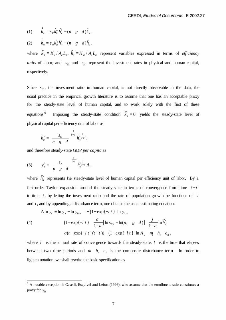
Since Hs , the investment ratio in human capital, is not directly observable in the data, the
usual practice in the empirical growth literature is to assume that one has an acceptable proxy
for the steady-state level of human capital, and to work solely with the first of these
equations.9 Imposing the steady-state condition ˆ 0itk =&
yields the steady-state level of
physical capital per efficiency unit of labor as 1
11ˆ ˆK
it it
sk h
n g
ϕαα
δ
−∗ ∗ −
= + +
,
and therefore steady-state GDP per capita as
(3) 1
1ˆKit it it
sy h A
n g
αϕαα
δ
−∗ ∗ −
= + +
,
where ith∗ represents the steady-state level of human capital per efficiency unit of labor. By a
first-order Taylor expansion around the steady-state in terms of convergence from time t τ−
to time t , by letting the investment ratio and the rate of population growth be functions of i
and t , and by appending a disturbance term, one obtains the usual estimating equation:
(4)
( )
( ) [ ]
( ) 0
ln ln ln 1 exp{ } ln
ˆ1 exp{ } ln ln( ) ln1 1
( exp{ }( )) 1 exp{ } ln ,
it it it it
Kit it it
i i t it
y y y y
s n g h
g t t A
τ τλτ
α ϕλτ δ
α α
λτ τ λτ µ η ε
− −
∗
∆ ≡ − = − − −
+ − − − + + + − − + − − − + − − + + +
where λ is the annual rate of convergence towards the steady-state, τ is the time that elapses
between two time periods and i t itµ η ε+ + is the composite disturbance term. In order to
lighten notation, we shall rewrite the basic specification as
9 A notable exception is Caselli, Esquivel and Lefort (1996), who assume that the enrollment ratio constitutes a proxy for Hs .
CERDI, Etudes et Documents, E 2002.27
8
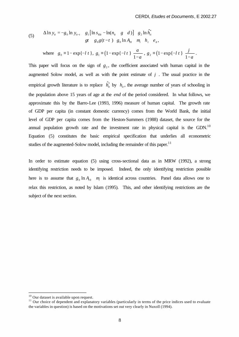
(5) [ ]0 1 2
0 0 0
ˆln ln ln ln( ) ln
( ) ln ,it it Kit it it
i i t it
y y s n g h
g g t Aτγ γ δ γ
τ γ τ γ µ η ε
∗−∆ = − + − + + +
+ + − + + + +
where ( ) ( )0 1 21 exp{ }, 1 exp{ } , 1 exp{ }1 1
α ϕγ λτ γ λτ γ λτ
α α≡ − − ≡ − − ≡ − −
− −.
This paper will focus on the sign of 2γ , the coefficient associated with human capital in the
augmented Solow model, as well as with the point estimate of ϕ . The usual practice in the
empirical growth literature is to replace ith∗ by ith , the average number of years of schooling in
the population above 15 years of age at the end of the period considered. In what follows, we
approximate this by the Barro-Lee (1993, 1996) measure of human capital. The growth rate
of GDP per capita (in constant domestic currency) comes from the World Bank, the initial
level of GDP per capita comes from the Heston-Summers (1988) dataset, the source for the
annual population growth rate and the investment rate in physical capital is the GDN.10
Equation (5) constitutes the basic empirical specification that underlies all econometric
studies of the augmented-Solow model, including the remainder of this paper.11
In order to estimate equation (5) using cross-sectional data as in MRW (1992), a strong
identifying restriction needs to be imposed. Indeed, the only identifying restriction possible
here is to assume that 0 0ln i iAγ µ+ is identical across countries. Panel data allows one to
relax this restriction, as noted by Islam (1995). This, and other identifying restrictions are the
subject of the next section.
10 Our dataset is available upon request. 11 Our choice of dependent and explanatory variables (particularly in terms of the price indices used to evaluate the variables in question) is based on the motivations set out very clearly in Nuxoll (1994).
CERDI, Etudes et Documents, E 2002.27
9
3. UNOBSERVED, COUNTRY-SPECIFIC HETEROGENEITY
Country-specific initial levels of technology
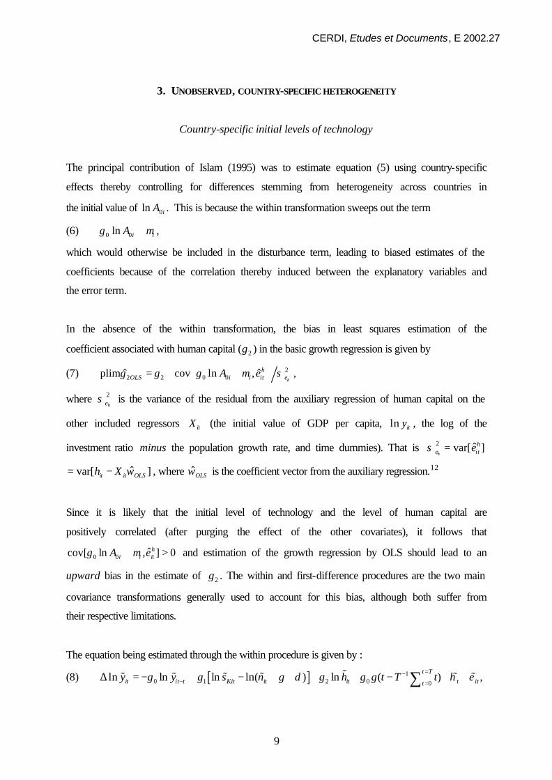
The principal contribution of Islam (1995) was to estimate equation (5) using country-specific
effects thereby controlling for differences stemming from heterogeneity across countries in
the initial value of 0ln iA . This is because the within transformation sweeps out the term
(6) 0 0ln i iAγ µ+ ,
which would otherwise be included in the disturbance term, leading to biased estimates of the
coefficients because of the correlation thereby induced between the explanatory variables and
the error term.
In the absence of the within transformation, the bias in least squares estimation of the
coefficient associated with human capital ( 2γ ) in the basic growth regression is given by
(7) 22 2 0 0ˆ ˆplim cov ln ,
h
hOLS i i it eA eγ γ γ µ σ = + + ,
where 2heσ is the variance of the residual from the auxiliary regression of human capital on the
other included regressors itX (the initial value of GDP per capita, ln ity , the log of the
investment ratio minus the population growth rate, and time dummies). That is 2he
σ ˆvar[ ]hite=
ˆvar[ ]it it OLSh X ω= − , where ˆOLSω is the coefficient vector from the auxiliary regression.12
Since it is likely that the initial level of technology and the level of human capital are
positively correlated (after purging the effect of the other covariates), it follows that
0 0 ˆcov[ ln , ] 0hi i itA eγ µ+ > and estimation of the growth regression by OLS should lead to an
upward bias in the estimate of 2γ . The within and first-difference procedures are the two main
covariance transformations generally used to account for this bias, although both suffer from
their respective limitations.
The equation being estimated through the within procedure is given by :
(8) [ ] 10 1 2 0 0
ln ln ln ln( ) ln ( ) ,t T
it it Kit it it t itty y s n g h g t T tτγ γ δ γ γ η ε
=−− =
∆ = − + − + + + + − + +∑% %% % % % %
CERDI, Etudes et Documents, E 2002.27
10
where 10
t Tit it i it itt
x x x x T x=−
• == − = − ∑% , represents variables expressed in terms of deviations
with respect to their country-specific means ( ix • represents variables in terms of their
country-specific means). Note that the entire term 10 0
( )t T
ttg t T tγ η
=−=
− +∑ % can be accounted
for by time specific dummies.13 The main weakness of the within transformation, as first
noted by Anderson and Hsiao (1981), is that the resulting estimator will be inconsistent if
some variables at time t are correlated with random shocks in any period s t≤ (some
elements of ix • will then be correlated with the error term). We shall return to this problem
later in the context of the issue of GMM estimation and autocorrelation.
An alternative means of eliminating the country specific effect is to first-difference the data.
This yields the equation
(9) [ ]
2
0 1 0 2
ln ln ln
ln ln ln( ) ln ,it it it
it Kit it it t it
y y y
y s n g g hτ
τγ γ δ γ τ γ η ε−
−
∆ = ∆ − ∆
= − ∆ + ∆ − ∆ + + + + ∆ + ∆ + ∆
where ln ln lnit it itx x x τ−∆ ≡ − and 2 ln ln lnit it itx x x τ−∆ ≡ ∆ − ∆ . This approach is similar to
that used by Hamilton and Monteagudo (1998), who estimate over two ten-year periods
(1960-70, 1975-85) using the MRW data, while allowing parameter estimates to vary by
decade.14 They then impose an increasingly stringent set of restrictions, ending up with a first-
differenced form that imposes the theoretical constraints suggested by the augmented Solow
model.15 Note that first-differencing results by construction in correlation between
2ln lnit ity yτ τ− −− (the differenced lagged-dependent variable) and it it τε ε −− (the differenced
error term), an issue that will be explicitly addressed below in the context of GMM
estimation. For the moment, this source of bias in the first-differenced results will be ignored.
Estimation results corresponding to pooling (estimation by OLS in levels), the within
procedure, and first-differencing are presented in columns (1), (2) and (3) of Table 2, and
largely reproduce those obtained by other authors (see the summary provided by Table 1). In
particular, we obtain a negative and statistically significant coefficient associated with human
capital using the within procedure and a negative and statistically insignificant coefficient in
12 Griliches and Hausman, 1986, p.97, Hsiao, 1986, p. 64, equation (3.9.3). 13 Alternatively, a second covariance transformation, in which variables are expressed as deviations with respect to time-specific means, will eliminate that portion of the disturbance term given by the previous expression. 14 Hamilton and Monteagudo (1998), equation 14, p. 500. 15 Hamilton and Monteagudo (1998), equation 15, p. 500, and equation 16, p. 502.
CERDI, Etudes et Documents, E 2002.27
11
first-differences. In Figures 1 through 3, we present graphs of the type popularized by Robert
Barro, in which the growth rate of GDP per capita, purged of the effects of all explanatory
variables except the variable of interest (education), is plotted on the vertical axis, with
education being plotted on the horizontal axis. The regression line also appears in the figure,
and passes through the origin by construction: its slope is equal to the value of 2γ (the
coefficient associated with human capital) estimated by each procedure.
Note that, despite what one might think in terms of what appear to be outliers (in Figures 2, 3
and 4), the unbounded nature of the influence function associated with the within and first-
difference estimators does not lie behind the negative 2γ coefficient. For example, when one
re-estimates the equation in first-differences by least absolute deviations (LAD), rather than
by least squares, a method that is robust to leptokurtic (i.e., “fat tailed”) disturbance terms,
and which is often used when one wishes to obtain results that are robust to outliers, the
estimated value of 2γ goes from 2ˆ 0.0125OLSγ = − with an associated t-statistic of -1.629, to
2ˆ 0.0188dLADγ = − with an associated t-statistic of -3.415 (the same result obtains, qualitatively,
when one estimates by LAD after the within transformation). Controlling for influential
observations therefore simply reinforces the puzzling negative coefficient associated with
human capital.16
These results highlight the main issue tackled by this paper, namely the instability of the sign
of the coefficient associated with human capital, which ranges from being positive and
statistically significant (pooling results), to being negative and statistically significant
(within).
At this point, it is worthwhile explicitly stating those hypotheses under which the within and
first-differenced results will be unbiased, as well as alternative, weaker, hypotheses that will
be considered at greater length in what follows.
ASSUMPTION 1 (exogeneity): [ln ] [ln( ) ] [ln ] 0, ,it is it is Kit isE h E n g E s s tε δ ε ε′ ′′= + + = = ∀ .
16 Temple (1999b) is able to obtain a positive coefficient on human capital on the Benhabib and Spiegel (1994) dataset, using OLS on first-differenced data, following use of least trimmed squares which allows him to eliminate 14 outliers. This specification does not, however, correspond to the augmented Solow model and involves only 64 observations (our first-differenced results involve 635 observations).
CERDI, Etudes et Documents, E 2002.27
12
ASSUMPTION 2 (predeterminedness) : [ln ]it isE y ε′ [ln ]it isE h ε′= [ln( ) ]it isE n g δ ε′= + +
[ln ]Kit isE s ε′= 0, s t= ∀ > .
ASSUMPTION 3 (correlated effects) : 0 0[ln ( ln )],it i iE h Aγ µ′ + 0 0[ln( ) ( ln )],it i iE n g Aδ γ µ′+ + +
0 0[ln ( ln )]Kit i iE s Aγ µ′ + 0≠ .
Both the within and first-differencing procedures are explicitly designed to deal with
ASSUMPTION 3 (correlated effects), and the within procedure will yield unbiased estimates
when ASSUMPTION 1 (exogeneity) holds. On the other hand, the within procedure will be
biased when ASSUMPTION 1 (exogeneity) is not satisfied, while first-differencing induces
correlation between the differenced lagged dependent variable and the differenced error term,
as previously noted, even when ASSUMPTION 1 is satisfied. ASSUMPTION 2
(predeterminedness) is crucial in allowing one to overcome this particular hurdle using
instrumental variable or GMM estimation. This issue will be addressed in section 4.
Country-specific rates of labor-augmenting technological change A potential source of bias not accounted for by Islam (1995) is constituted by country-specific
rates of technological progress.17 Consider the basic growth regression, which may now be
expressed as:
(10) [ ]0 1 2
0 0 0
ln ln ln ln( ) ln
( ) ln ,it it Kit it i it
i i i i t it
y y s n g h
g g t Aτγ γ δ γ
τ γ τ γ µ η ε−∆ = − + − + + +
+ + − + + + +
where the difference with equation (9) is that g has been replaced with the country-specific
growth rate of labor productivity ig . In order to assess the magnitude of the bias induced by
failure to control for differences in ig , consider a first-order Taylor expansion around itn δ+ ,
which allows one to write 1ln( ) ln( ) ( )it i it it in g n n gδ δ δ −+ + = + + + . It follows that the basic
growth regression can be rewritten as:
[ ]0 1 2
11 0 0 0
ln ln ln ln( ) ln
( ) ( ) ln .it it Kit it it
it i i i i i t it
y y s n h
n g g g t Aτγ γ δ γ
γ δ τ γ τ γ µ η ε−
−
∆ = − + − + +
− + + + − + + + +
Neither the within procedure nor first-differencing eliminates this source of bias. In the case
of the within procedure, the term
CERDI, Etudes et Documents, E 2002.27
13
( ) ( )1 1 1 10 10 0
( ) ( )t T t T
it i i it itt tg t T t g n T nϑ γ γ δ δ
= =− − − −= =
= − − + − +∑ ∑
remains, leading to a bias given by
(11) 22 2ˆplim cov[ , ]
h
hw it it eeγ γ ϑ σ= +
%
% ,
where 2 ˆvar[ ] var[ln ]h
he it it it we h Xσ ω= = −
%
% % % is the variance of the residual from the auxiliary
regression of human capital on the other regressors using the within procedure. Similarly, the
equation to be estimated by least squares after first-differencing is now given by
(12) [ ]2
0 1 2
11 0
ln ln ln ln( ) ln
( ) ,it it Kit it it
i it i t it
y y s n h
g n gτγ γ δ γ
γ δ γ τ η ε−
−
∆ = − ∆ + ∆ − ∆ + + ∆
− ∆ + + + ∆ + ∆
with the bias being given by
(13) ( )1 22 2 0 1ˆplim cov ( ) ,
h
hd i it it eg n eγ γ γ τ γ δ σ
∆
− ∆ = + − ∆ + ,
where 2 ˆvar[ ] var[ ln ]h
he it it it de h Xσ ω∆
∆= = ∆ − ∆ is the variance of the residual from the
corresponding auxiliary regression. Since it is likely that the level of human capital is
positively correlated with the country-specific rate of technological progress, failure to
account for this problem is likely to bias estimates of the impact of human capital on growth
upwards.18
The solution to this problem is to move to second-differences, which will eliminate 0 igγ τ
from equation (12), and to assume multiplicative country-specific fixed effects to account for
the remaining source of heterogeneity ( 2 11 ( )i itg nγ δ −∆ + ) since the equation to be estimated by
least squares is now given by:
(14) 3 2 2 2 2
0 1 2
2 1 2 21
ln ln ln ln( ) ln
( ) .
it it Kit it it
i it t it
y y s n h
g n
τγ γ δ γ
γ δ η ε
−
−
∆ = − ∆ + ∆ − ∆ + + ∆ − ∆ + + ∆ + ∆
Note that, if second-differencing alone is performed, the bias will be equal to
1 22 2 1ˆplim cov ( ) ,
h
hd it i it en g eγ γ γ δ σ
∆
− ∆ = + − ∆ + .
17 This issue is considered explicitly by Lee, Pesaran and Smith (1998) who consider a stochastic version of the Solow growth model. It is also worth emphasizing that the assumption of country-specific rates of technological change is linked to the debate concerning σ -convergence. 18 More precisely, and as with the bias stemming from uncontrolled for differences in the initial level of technology, we assume that the residual from the auxiliary regression is, like human capital itself, positively correlated here with the country-specific rate of technological change.
CERDI, Etudes et Documents, E 2002.27
14
Estimates of the parameters of the growth regression in second-differences and in second-
differences with multiplicative country-specific effects are presented in columns (6) and (7) of
Table 2. Figure 4 presents a Barro-type graph corresponding to the second-differenced results.
Note that there is some evidence that the specification in terms of labor-augmenting
technological change employed in the basic MRW specification is itself misplaced. Boskin
and Lau (2000) find, for the G7 countries, that "technical progress is simultaneously purely
tangible capital and human capital augmenting, that is, generalized Solow-neutral….
Technical progress has been capital, not labor, saving." On the other hand, this should not
present particular problems in the context of empirical implementations of the augmented
Solow model since different forms of technological progress cannot be identified.19
It is also worth noting that other sources of unobserved heterogeneity can readily be found in
the augmented Solow model. The most obvious stems from the linearization around the
steady-state used to move from equation (3) (the steady-state level of GDP per capita) to
equation (4) (the basic growth regression). This is because, while it is customary to write the
annual rate of convergence towards the steady as a constant ( )(1 )n gλ δ α ϕ= + + − − , one
should really be writing ( )(1 )it itn gλ δ α ϕ= + + − − . The speed of convergence should
therefore vary over time. It should also vary across countries.
The first problem is considered implicitly by Hamilton and Monteagudo (1998), who allow
for coefficients that vary over the two time periods of their estimations.20 It is also dealt with
partially by Rappaport (1999), who explicitly considers variations over time in the speed of
convergence, although his empirical specification is chosen (rightly, in his case) for its
tractability rather than its faithfulness to the theoretical construct of the Solow model. The
second problem (country-specific rates of convergence) is implicitly tackled in Durlauf,
Kourtellos and Minkin (2001) in that their non-parametric approach allows all coefficients to
19 In the basic augmented Solow specification, if we change the production function so that it is specified in terms of Solow-neutral technological change, 1( )Y A K H Lit it it it it
ϕ α ϕα − −= , with all other assumptions remaining the
same, the country-specific term in the growth regression becomes [(1 )/(1 )]ln 0Ai iϕ α µ+ − + . The within procedure
or first-differencing will therefore eliminate this source of bias. The same discussion goes for country-specific rates of technological change in the second-differencing procedure. Note, however, that the magnitude of the bias stemming from the failure to account for country-specific effects will be changed by dint of the fact that the country-specific term is now multiplied by (1 )/(1 )ϕ α+ − . 20 Hamilton and Monteagudo (1998), equation 9, p. 498 in theoretical terms, equation 14, p. 500 for the empirical results.
CERDI, Etudes et Documents, E 2002.27
15
vary over countries, as a function of the initial level of GDP per capita. However, as they do
not seek to impose the restrictions implied by the Cobb-Douglas functional form, they do not
furnish one with estimates of country-specific heterogeneity in the rate of convergence. It is
interesting to note, in terms of the human capital puzzle, that their estimate of 2γ is positive
for values of log GDP per capita lying roughly between 6.3 ($544) and 7.5 ($1,808), and is
negative otherwise.21
Simple covariance transformations and the coefficient associated with human capital: lessons learned
The upshot of these three simple covariance transformations, and the likely direction of bias
induced by the failure to control for unobserved country-specific heterogeneity in pooling
regressions or cross-sectional studies, is that there is probably significant positive bias
introduced by failure to control for differences in 0iA and ig . The fact that the coefficient
associated with human capital goes from being positive to being negative (as well as the fact
that the point estimate of α is significantly reduced –similar expressions for the bias in the
coefficient associated with physical capital hold) is evidence enough of that. However, given
that the estimates of ϕ are either negative and statistically significant, or statistically
indistinguishable from zero, there must be other sources of bias, not controlled for by the
within, first-differencing, or second-differencing procedures, which bias estimates of ϕ
downwards. Moreover, these potential sources of bias may be exacerbated by the procedures
in question. The natural candidate is of course measurement error in the human capital
variable.
4. MEASUREMENT ERROR
As with most authors, we use the measure of the stock of human capital (average number of
years of schooling in a given population) constructed by Barro and Lee (1993, 1996). This
variable was generated partly by using census information on school attainment.
Unfortunately, available census data only give information for a subset corresponding to 40
21 Durlauf, Kourtellos and Minkin (2001), Figure 1, p. 934. An additional source of bias in the standard tests of the augmented Solow model involves the imposed functional form. Duffy and Papageorgiou (2000) show that a CES functional form is preferred over the usual Cobb-Douglas specification, although they use a human capital adjusted measure of the labor input (i.e. education does not enter as a separate input or, more precisely, its coefficient is restricted to being the same as that associated with labor) and do not consider the augmented Solow

CERDI, Etudes et Documents, E 2002.27
16
percent of time periods. Barro and Lee were therefore obliged to infer missing data from
enrollment ratios (as well as from adult illiteracy rates which allows one to construct a good
proxy of the no-schooling category). As noted by Krueger and Lindahl (2001), and many
other authors, “errors in measurement are inevitable because the enrollment ratios are of
doubtful quality in many countries...errors cumulate over time, the errors will be positively
correlated over time.”22 For the time being, the serial correlation aspect of the Barro-Lee
human capital variable, as well as the impact of any serial correlation that there may be in the
associated measurement error will be ignored: our focus, in this section, will be on the
classical measurement error problem.23
Assume that one observes an error-ridden measure of human capital ith′ given by the true
value of human capital ith plus an error term :
ASSUMPTION 4 (classical measurement error):ln lnit it ith h u′ = + , where itu is distributed i.i.d.
with mean zero and variance 2uσ .
ASSUMPTION 4 (classical measurement error) implies that the bias in the coefficient associated
with human capital is given by
(15) 2 2 2 22 2 2ˆplim cov[ , ] ( 1) ( ) ,
h h
hw it it e u e ue T Tγ γ ϑ σ γ σ σ σ = + − − + % %
%
in the case of the within estimator, and by
(16) ( )1 2 2 2 22 2 0 1 2ˆplim cov ( ) , 2 ( )
h h
hd i it it e u e ug n eγ γ γ τ γ δ σ γ σ σ σ
∆ ∆
− ∆ = + − ∆ + − +
in the case of the first-difference estimator (there is simply an extra term in each equation
with respect to the expressions given in equations (11) and (13)). In the case of second-
differences with multiplicative country-specific effects, the bias should be equal to
(17) 2
2 2 222 2 2ˆplim 4 ( )
hd u e uγ γ γ σ σ σ
∆= − + ,
where 2
22 2
22ˆvar[ ] var[ ln ]hit it it dh
e e h X ω∆=
∆= ∆ − ∆ . These three expressions are standard
examples of attenuation bias stemming from an errors in variables problem. Computing the
model per se since their focus is on an aggregate production function. 22 Nehru, Swanson and Dubey (1995) provide an alternative measure of the human capital stock that is sometimes used in empirical studies of the augmented Solow model (see, e.g. Temple, 1999a). 23 Temple (1999b) considers the robustness of the MRW cross-sectional results to classical measurement error, using the Klepper and Leamer (1984) reverse regression technique as well as classical method of moments estimators (Carroll, Ruppert and Stefanski, 1995). He does not, however, consider the robustness of the panel data literature. He finds that estimates of ϕ lie between 0.15 and 0.38 (p. 371).
CERDI, Etudes et Documents, E 2002.27
17
attenuation bias due to measurement error is much more complicated in the case where
several variables are affected. Nelson (1995) shows that the vector of OLS parameters is also
asymptotically biased towards zero. While this does explain why the coefficient associated
with human capital might be biased downwards, it implies that, far from being overestimated,
the coefficient associated with physical capital may be underestimated (the opposite of what
is usually believed).
Note that it may be the case that the two sources of bias (upward from the failure to control
for unobserved country-specific heterogeneity, downward for measurement error) cancel each
other out in the pooling results. A similar argument could be made for the remaining
unobserved heterogeneity stemming from ig and measurement error on human capital in the
within and first-difference estimations; the fact that the coefficient associated with human
capital is negative would suggest that the downward bias from measurement error
overwhelms the upward bias from ig in these estimations. Simply controlling for unobserved
heterogeneity stemming from uncontrolled for differences in 0iA and iµ by the within
procedure or first-differencing leaves the negative measurement error bias intact (moreover, it
worsens it with respect to the corresponding expression for the pooling estimator in that the
denominator falls, since 2 2h he eσ σ
∆< —more on this fall in variance in section 5). This might
be conjectured to be a reason why the pooling results yield a reasonable, that is positive,
estimate of ϕ whereas correcting for unobserved heterogeneity in 0iA and iµ yields a
negative ϕ .
Within versus first-differences: estimating the magnitude of the bias due to measurement error
Can anything be said concerning the magnitude of the bias in the estimates of 2γ stemming
from classical measurement error using the simple covariance transformations that have been
the subject of the paper up until now? As is well-known (Griliches and Hausman, 1986),
different covariance transformations that control for the country-specific fixed effect can be
combined in order to obtain consistent estimators for 2γ and 2uσ . In particular, when one
combines the first-difference and within estimators, one obtains:24
24 Hsiao, 1986, p. 65, equations (3.9.8) and (3.9.9); similarly, there are / 2 1 3T − = other estimators, using other “long” differences, that allow one to deduce the magnitude of the bias.
CERDI, Etudes et Documents, E 2002.27
18
(18)
1
2 22 2 2 2 2
ˆ ˆ2 ( 1) 2 ( 1)ˆh hh h
w d
e e e e
T TT T
γ γγ
σ σ σ σ∆ ∆
− − −
= − − % %
, 2
2 2 2
2
ˆ ˆˆ
ˆ 2hed
u
σγ γσ
γ∆ −
=
.
Computing the empirical counterparts to equation (18) on the basis of the results presented in
columns 2 and 3 of Table 2 yields 2γ = -0.2247 and 2ˆuσ = 0.006. Combining the two
covariance transformations therefore still leads us to a negative point estimate for 2γ , which
runs counter to common sense. Part of the answer to this additional puzzle must surely lie in
the relative magnitudes of the within and first-difference coefficients: it is usually expected
that the bias is greater in the within than in the first-difference results, although here (if the
true coefficient is positive) the opposite obtains. This means that one or more of the
maintained assumptions needed to implement the Griliches and Hausman approach must be
violated. The problem is that it is impossible to say at this stage which one it is.
The issue of the potential for sign-reversal induced by the two covariance transformations
brings this question into sharper focus. If one ignores the bias stemming from unobserved
country-specific heterogeneity in the within results, classical measurement error per se cannot
explain a reversal of the sign of the coefficient since, from equation (15), one can deduce that
2ˆsign[plim ]wγ 2 2 2 22sign[ ( ) / ( )]
h he u e uT Tγ σ σ σ σ= + +% % 2sign[ ]γ= . In the case of the first-difference
estimator, on the other hand (and again ignoring the bias stemming from failure to account for
country-specific ig ), the formula given in equation (16) implies that it suffices that 2 2he uσ σ
∆<
for sign reversal to obtain. It follows that, while classical measurement error can explain a
statistically insignificant coefficient associated with human capital in the within results, it
cannot explain a statistically significant negative coefficient, if one accepts the basic
hypothesis that the true coefficient is indeed positive. On the other hand, classical
measurement error can account for the sign reversal that appears in the first-difference results,
since the first-difference transformation will result (usually) in a large reduction in the
variance of the human capital variable. This last issue will be explored at much greater length
in section 5.
A further indication of the presence of measurement error: the impact of correcting for serial correlation in the first-differenced results
As was first noted by Grether and Maddala (1973), and more recently by Dagenais (1994), the
combination of serially correlated errors in the equation’s disturbance term ( itε in equation
CERDI, Etudes et Documents, E 2002.27
19
(5)) and measurement error in one of the variables (human capital) can lead to extremely
puzzling results when corrections for serial correlation are carried out. Assume that the
disturbance term in the growth regression follows a first-order autoregressive process:
1it it itεε ρ ε ξ−= + , where itξ is white noise.
If human capital were the only variable in the regression, and if it and the measurement error
are not serially correlated (ASSUMPTION 4, classical measurement error), the bias in 2γ
induced when one corrects for serial correlation in the presence of measurement error
(ignoring unobserved country-specific heterogeneity) is exactly the same as given above (for
example, equation (17)). On the other hand, if one assumes that human capital is serially
correlated, with
(19) 1it h it ith hρ ζ−= + ,
where itζ is white noise, the expression for bias becomes:25
(20) 2 2
22 2 2 2 2
(1 2 )ˆplim(1 2 ) (1 )
h h
h h u
ε ε
ε ε ε
γ σ ρ ρ ργ
σ ρ ρ ρ σ ρ
∗ ∗
∗ ∗ ∗
+ −=
+ − + +,
where 2 2 2 2 2 2 2 2
22 2 2 2 2 2 2 2
2
( ) ( )( )[ ( ) ]
h u u h h
u h h u u h
ε εε
ε
ρ σ σ σ γ σ ρ σρ
σ σ σ σ σ γ σ σ∗ + +
=+ + +
.
It should be apparent from equation (20) that bias which induces sign reversal is a possibility,
if one corrects for serial correlation (it suffices for the numerator to be negative and the
denominator to be positive, which is entirely possible). Moreover, Dagenais shows that the
bias induced by correcting for serial correlation is increasing in the ratio of the variance 2uσ of
the measurement error to the variance 2hσ of the true variable. When one re-estimates the
pooling regression (column (1) in Table 2) while correcting for first-order serial correlation,
the parameter estimates change very little.26 In light of the previous comments, this may be
taken as indication that the variance of the measurement error is relatively small with respect
to the variance of the education variable in levels.
On the other hand, when one re-estimates the regression in first-differences while correcting
for first-order serial correlation (in the first-differenced residuals), the change in the point
25 See Dagenais (1994), equations (10)-(12), p. 155, for the general case in which the measurement error is itself serially correlated. 26 Not presented but available upon request.
CERDI, Etudes et Documents, E 2002.27
20
estimates is impressive.27 In particular, the coefficient associated with human capital more
than doubles (in absolute value), and becomes statistically significant at the usual levels of
confidence. Results are presented in column (4) of Table 2. What can be inferred from this
last finding ? Assume that the disturbance term of the growth regression in first-differences
follows a first-order autoregressive process: 1it it itεε ρ ε ξ∆ −∆ = ∆ + , where itξ is white noise.
Then an expression similar to equation (20) obtains where we substitute 2hσ ∆ , 2
ερ ∗∆ , hρ∆ , and
2uσ ∆ for their counterparts in levels. The implication is that the variance of the measurement
error is relatively large with respect to the variance of the education variable, when both are
expressed in first differences. Of course, while this result does indicate that measurement
error is a potentially serious problem, we are still left with the puzzle of why sign-reversal
obtains in the absence of correcting for serial correlation.
Instrumental variables estimation
The traditional cure for an errors in variables problem is, of course, estimation by
instrumental variables. Concomitantly, we now return to the issue of the correlation, induced
by first-differencing, between the first-differenced disturbance term and the first-differenced
lagged dependent variable, that was mentioned earlier. Again, the standard cure, first
advocated by Anderson and Hsiao (1981), involves instrumental variables estimation.
Recall, from equation (9), that first-differencing induces correlation between
2ln ln lnit it ity y yτ τ τ− − −∆ = − and it it it τε ε ε −∆ = − , since ln ity τ− is correlated with it τε − . We
now make the following identifying assumption:
ASSUMPTION 5 (no autocorrelation in the error term): [ ] 0,it isE s tε ε = < .
In the absence of serial correlation in itε , and under ASSUMPTION 2 (all right-hand-side
variables are predetermined) a valid instrument for ln ity τ−∆ is given by 2ln ity τ− . This is
because 2ln ity τ− is orthogonal to it it it τε ε ε −∆ = − (if itε were autocorrelated, this would no
27 We present evidence below in the context of Arellano-Bond GMM estimation that the residuals of the growth regression in first-differences are indeed serially correlated of order one, although this serial correlation is negative.
CERDI, Etudes et Documents, E 2002.27
21
longer be the case because one could write 2it it itτ ε τ τε ρ ε ξ− − −= + , with it τξ − white noise and
2ln ity τ− would no longer be orthogonal to 2( )it it it it itε τ τ τε ρ ε ε ξ ξ− − −∆ = − + − ). Moreover,
given ASSUMPTION 5, 3ln ity τ− is also a valid instrument for ln ity τ−∆ , as is any ln , 2it ny nτ− ≥ .
This is expressed by the following orthogonality condition:
ASSUMPTION 6 (orthogonality condition on lagged dependent variable):
[ln ]it n itE y τ θ−′∆ 0, 2n= ≥ ,where itθ∆ t itη ε= ∆ + ∆ 2
0ln lnit ity y τγ −= ∆ + ∆
[ ]1 ln ln( )Kit its n gγ δ− ∆ − ∆ + + 2 0ln ith gγ γ τ− ∆ − .
In terms of the other explanatory variables, we pose the following additional orthogonality
conditions, which simply formalize ASSUMPTION 2 (predeterminedness) in GMM
terminology :
ASSUMPTION 7 (orthogonality conditions on explanatory variables): [ln ]it n itE h τ θ−′′ ∆
[ln( ) ] [ln ] 0, 2it n it Kit n itE n g E s nτ τδ θ θ− −′′= + + ∆ = ∆ = ≥ .
Note that using the human capital variable lagged two periods and more as instruments will
be valid only when ASSUMPTION 4 and ASSUMPTION 5 both hold, that is when there is no
autocorrelation in the disturbance term in the growth regression and well as no autocorrelation
in the measurement error affecting human capital. Autocorrelation in itε renders the
explanatory variables lagged two periods inadmissible as instruments for the same reasons as
for 2ln ity τ− . On the other hand, autocorrelation in the measurement error, which one may
write as ln lnit it ith h u′ = + , where it u it itu u τρ υ−= + , with itυ white noise, implies that
1 12it u it u itu uτ τ τρ ρ υ− −
− − −= − . Since ASSUMPTION 7, for the specific case of the human capital
variable, may be written as 2 2[(ln ) ( )] 0it it t it itE h uτ τ τη ε ε− − −′+ ∆ + − = , substitution implies that
2
1 12[(ln ) ( )] 0
it
it u it u it t it it
h
E h uτ
τ τ τ τρ ρ υ η ε ε−
− −− − − −
′
′+ − ∆ + − ≠1444442444443 ,
since itu τ− is correlated with it τε − . Autocorrelation in the measurement error therefore results
in a violation of the orthogonality condition given by ASSUMPTION 7.
CERDI, Etudes et Documents, E 2002.27
22
Current econometric technique combines the instruments defined by ASSUMPTIONS 6 and 7 in
an optimal manner through the use of the generalized method of moments (GMM) estimator.
The key to understanding the GMM approach, pioneered by Arellano-Bond (1991a, 1991b), is
to note that the number of lags that may be used as instruments depends upon the time
dimension of the panel. In the case at hand, 8T = . Formally speaking, we set up the problem
as a set of 6 growth regressions in first-differences because: (i) the first time period is lost
through first-differencing ( 1T − ) and (ii) two additional time periods are lost because the
minimal set of instruments is constituted by the explanatory variables lagged two periods,
although we retrieve the period lost through first-differencing in terms of instruments
( 1 2 1 6T − − + = ). These six equations are estimated as a system, imposing the restrictions
that the coefficients are equal across equations. In our notation, the system of equations is as
follows, where we indicate the set of valid instruments for each equation in parentheses:
[ ]
[ ]
20 0 1 2
24 0 0 5 1 4 4 2 4 4
7
ln ln ln ln( ) ln
(instruments ln ,ln , 2,...,7)
ln ln ln ln( ) ln
(instruments ln
it it Kit it it it
it n it n
it it Kit it it it
it
y g y s n g h
y x n
y g y s n g h
y
τ
τ τ
τ τ τ τ τ τ
τ
γ τ γ γ δ γ θ
γ τ γ γ δ γ θ
−
− −
− − − − − −
−
∆ = − ∆ + ∆ − ∆ + + + ∆ + ∆
= =
∆ = − ∆ + ∆ − ∆ + + + ∆ + ∆
=
M M
[ ]7 6 6
25 0 0 6 1 5 5 2 5 5
7 7
,ln ,ln ,ln )
ln ln ln ln( ) ln
(instruments ln ,ln )
it it it
it it Kit it it it
it it
x y x
y g y s n g h
y x
τ τ τ
τ τ τ τ τ τ
τ τ
γ τ γ γ δ γ θ− − −
− − − − − −
− −
∆ = − ∆ + ∆ − ∆ + + + ∆ + ∆
=
This means that for those observations where 5ln ity τ−∆ is regressed on 6ln ity τ−∆ and 5ln itx τ− ,
7ln ity τ− and the matrix of explanatory variables 7ln itx τ− are the admissible instruments,
whereas for those observations where 4ln ity τ−∆ is regressed on 5ln ity τ−∆ and 4ln itx τ− ,
7ln ity τ− and 6ln ity τ− are both admissible, as are 6ln itx τ− and 7ln itx τ− , and so on as one moves
forward in time.
A well-known example of the application of this estimator to the augmented Solow model is
the paper by Caselli, Esquivel and Lefort (1996), who find, estimating over the 1960-1985
time period with 5τ = and 5T = : (i) substantially higher rates of convergence than was
previously found using conventional panel techniques ( ˆ 0.10λ ≈ ), (ii) an implied capital share
that is much more in line with conventional wisdom than those obtained using simple cross-
sections ( ˆ 0.49α ≈ ) and, unfortunately, (iii) a negative and statistically significant coefficient
CERDI, Etudes et Documents, E 2002.27
23
associated with the human capital variable ( ˆ 0.25ϕ ≈ − ).28 On the basis of this last finding,
Caselli, Esquivel and Lefort (1996) reject the augmented Solow model outright.
Caselli, Esquivel and Lefort (1996) are careful to test for first-order serial correlation in the
disturbance term in the growth equation which, in the presence of measurement error in the
human capital variable, is equal to 2 it ituγ ε+ . The absence of first-order serial correlation in
the disturbance term of the growth equation in levels is implied, in the growth equation
expressed in first-differences, by : (i) the presence of negative first-order serial correlation
and (ii) the absence of second-order serial correlation:29 they cannot reject the null hypothesis
that ASSUMPTIONS 4 and 5 hold. This last statement follows because the absence of serial
correlation in the composite disturbance term 2 it ituγ ε+ implies its absence in both of its
components.30
As a further test for the presence of autocorrelation in the measurement error, Caselli,
Esquivel and Lefort (1996) re-estimate their specification while dropping the most recent
instruments. They show that the results are not very different according to whether they use
the restricted or unrestricted matrix of instruments.31
In the first column of Table 2, we present results corresponding to application of the Arellano-
Bond estimator to our data. Our results are similar to those of Caselli, Esquivel and Lefort
(1996), in that our estimate of ϕ is negative and highly significant. Moreover, the situation is
even worse in that the point estimate is twice that found by Caselli, Esquivel and Lefort. As
with their specification, the Sargan test of the overidentifying restrictions strongly rejects the
specification, with a p-value coming in at the 3 percent level. Manifestly, the Arellano-Bond
estimator does not provide one with a solution to the human capital puzzle. As we shall see
28 Caselli, Esquivel and Lefort, 1996, Table 3, p. 376. 29 Arellano and Bond, 1991a, pp. 281-2. 30 Note that some authors reject the use of lagged right-hand-side variables altogether as instruments, even in the absence of serial correlation concerns. For example, Rappaport (2000) notes that “the potential for a reverse causal link from the current income level to any of the “stock” conditioning variables (i.e., right-hand-side variables constrained to a finite time derivative) ” should be of great concern in any instrumental variable procedure based on the Arellano-Bond approach. As he puts it: “To the extent that an included right-hand-side stock variable is a normal good, its level will increase with income; education and public capital seem obvious examples. The persistence of stock variables along with optimization by forward-looking agents rule out using lagged values as instruments” (Rappaport, 2000, p. 13). 31 A further development on the methodology implemented by Caselli, Esquivel and Lefort (1996) is provided by Bond, Hoeffler and Temple (2001), who use the system GMM estimator proposed by Arellano and Bover (1995) and Blundell and Bond (1998). This approach combines equations in levels with those in first-differences,
CERDI, Etudes et Documents, E 2002.27
24
below, part of the problem lies in the low variability of the human capital variable once first-
differencing is performed, with an additional source of difficulty probably stemming from the
weakness of the instruments used in the standard GMM procedure. It is this “weak
instrument” problem that the new estimator introduced in the next section is designed to
overcome.
5. LOW VARIABILITY IN THE HUMAN CAPITAL VARIABLE
There are two additional standard reasons that could explain the lack of significance of the
human capital variable (though not sign-reversal per se) once country-specific effects have
been accounted for through a covariance transformation such as first-differencing. The first
involves multicollinearity induced by the covariance transformation. The second involves a
reduction in the variance of the human capital variable following the covariance
transformation. This is because the least squares estimate of the variance of 2ˆ wγ is given by
2 2 22ˆvar[ ] / (1 )w h hRεγ σ σ= −% %% , where 2
hR% is the R-squared of the auxiliary regression of human
capital on the other explanatory variables and 2hσ % is the variance of the human capital variable
after the covariance transformation.
The term 2 1(1 )hR −− % , which is known as the variance inflation factor (VIF), is a measure of the
collinearity that exists between human capital and the other included regressors.32 If the
degree of collinearity is high, 2ˆvar[ ]wγ will be large, ceteris paribus. Similarly, if the
covariance transformation results in a dramatic fall in 2hσ % with respect to 2
hσ (its counterpart
in levels), then again, 2ˆvar[ ]wγ will be large when compared with 2ˆvar[ ]OLSγ .33 If we
consider the pooling and the within results, the VIFs are almost identical in that the 2R of the
auxiliary regressions come in at 0.6676 for the pooling regression and 0.6675 for the within
regression. It is therefore not an increase in collinearity stemming from the within
transformation that is driving the human capital puzzle.
where the variables in the equations in levels are instrumented using twice lagged first-differenced variables. 32 We include the VIF for the human capital variable for all estimations presented in Table 2, as well as the variance of the residuals of the auxiliary regression of human capital on the other explanatory variables. 33 When we speak of a reduction in
2hσ % , we mean of course, a reduction with respect to 2
εσ % .
CERDI, Etudes et Documents, E 2002.27
25
On the other hand, the within transformation does result in a substantial reduction in the
variance of the human capital variable, which goes from 2hσ = 0.6935 in levels to 2
hσ =% 0.1321
after the within transformation. Removing country-specific means therefore does result in a
substantial loss in the variance that could be the cause of insignificant coefficients associated
with the human capital variable. The situation is even worse when one carries out first-
differencing, with 2hσ ∆ = 0.0230. This dramatic fall in variance is illustrated in Figure 5,
where we plot different kernel density estimates of the human capital variable following
various transformations (all variables have had their unconditional mean subtracted, which
explains why all the kernels are centered on zero): it is obvious that the within and first-
difference transformations correspond to substantial mean-preserving decreases in the
"spread" (in the sense of Rothschild and Stiglitz) of the distribution of ln ith , with respect to
the situation in levels (graphically, the estimated distributions become much more
concentrated around zero). As one would expect from the respective variances reported
above, this decrease in the spread is much more noticeable for the first-difference
transformation than for the within transformation.
In order to counter this problem, Mairesse (1990, p. 92, 1993, p. 435) suggests carrying out a
"between" estimation after performing the first-difference transformation. The first step
eliminates the country-specific effect, while the second should ensure that variables expressed
in first-differences recover sufficient variance for their effect to be identifiable. In terms of
the problem at hand, this approach will be worthwhile only if the second transformation
allows one to recoup a sufficient amount of variance: this is not the case, since the variance of
the education variable after the second transformation falls once again, to 2b hσ ∆ = 0.0060.
Results corresponding to the between regression on first-differences are presented in column
5 of Table 2. Once again, the procedure in question does not solve the human capital puzzle.
The growth process of human capital
The preceding findings in terms of the variances associated with various covariance
transformations of the human capital variable naturally leads one to investigate its statistical
properties more closely. Recall that the within transformation purges the human capital
variable of its country-specific mean over the period. All that remains are within-country
changes in human capital, and if that rate of growth is roughly constant (the variable is in
CERDI, Etudes et Documents, E 2002.27
26
logs), the within transformation will have removed inter-country differences due to
differences in the initial level of education, leaving only relatively small differences in the
between-period growth rate of human capital. The same is true of the first-difference
transformation. In order to illustrate this point formally, consider the following exponential
growth process for human capital: 0 exp{ }it i ih h a t= which implies that
(21) 0ln lnit i ih h a t= + ,
where 0ih is the (country-specific) initial level of human capital, and ia is its (country-
specific) growth rate. If we consider the first-difference transformation, equation (9) may
then be re-expressed as :
(22) [ ]20 1 0 2ln ln ln ln( ) .it it Kit it i t ity y s n g g aτγ γ δ γ τ γ τ η ε−∆ = − ∆ + ∆ − ∆ + + + + + ∆ + ∆
What is clear in equation (22) is that the entire effect of human capital in the regression will
be identified through the variations in ia .34 How great can one expect the fall in variance of
the human capital variable to be when one moves from estimation in levels to estimation in
first-differences, when human capital follows the process defined by (21)? Let 2var[ ] ,i aa σ=
and 0
20var[ln ]i hh σ= . Then it can be shown that the variance of the logarithm of human
capital in a pooling regression over T periods is given by:
0
12 2 2 2 21
( 1)t
n Th h a n
T nσ σ τ σ= −
== − + ∑ .35
Now consider a regression in first-differences. The variance of the first-difference of the
logarithm of human capital, where the equation is estimated over 1T − periods, is given by: 2 2 2( 1)
th aTσ τ σ∆ = − .
The ratio of the variances of log human capital in levels and log human capital in first-
differences is therefore given by:
(23) 0
2 22 2
2 2 2 1
11
1t
t
n Th h
nh a
n TT
σ σ
σ τ σ= −
=∆
= + + −− ∑ .36
34 Note that, if this were indeed the true process generating human capital, the effect of the latter would not be identifiable at all in the equation estimated in second-differences ? this is indeed what happens, in the sense that the standard error associated with human capital becomes extremely large when one moves to second-differences; see the results presented in Table 2, column 6. 35 See APPENDIX 1 for the derivation. 36 It is interesting to note that this expression provides part of the explanation for why the coefficients (and especially their standard errors) vary as the time frame (2 twenty-year periods, 4 ten-year periods, etc.) over which growth regressions in first differences are estimated changes.
CERDI, Etudes et Documents, E 2002.27
27
Here 5τ = and 8T = which implies that 0
2 2 2 2/ 20 ( /25 )t th h h aσ σ σ σ∆ = + . Thus, if human capital
follows the process given by (21), one expects the variance that is performing the function of
identification to fall by a factor of at least 20. This is indeed what happens when one
performs the first-difference transformation: the resulting ratio of variances is approximately
equal to 30 (here 0
21960var[ln ]i hh σ= = 1.013).
How good an approximation of the behavior of the human capital variable is the process
described by equation (21)? In order to assess its empirical validity, we simply performed the
regression suggested by (21), thereby estimating country-specific, time-invariant growth rates
of human capital. For the regression in question 2R = 0.8519, and the resulting estimate of 2aσ is equal to 0.00029 (the F-test associated with the null-hypothesis that the estimated ˆia
are equal across countries, and thus that 2 0aσ = , is rejected with a p-value below 0.001). If
we constrain the growth rates to be equal ( i ja a a= = and thus 2 0aσ = ), the mean rate of
growth of human capital is equal to 0.024 per five-year period. The results are represented
graphically in Figure 6, where we plot the actual value of ln ith against the value predicted by
(21): as should be obvious from the Figure, the fit is extremely good.
Note that the preceding argument is a powerful explanation for the imprecision of the
estimates of the coefficient associated with human capital, after the first-difference
transformation. It does not, however, explain a negative and statistically significant
coefficient. In order to do so, measurement error must again be invoked. If the measurement
error takes a form such that its magnitude is relatively important, relative to that of the
transformed human capital variable, then (i) the process generating the human capital
variable, (ii) measurement error and (iii) the first-difference transformation which results in a
dramatic fall in the variance of the human capital variable may explain the negative
coefficient associated with human capital.
Suppose that there is measurement error in the country-specific growth rate of human capital.
We pose this as follows:
0ln ln ( ) ,it i i ith h a tθ′ = + + where itθ is i.i.d. 2(0, )N θσ: .
Under this assumption, the equation in first-differences is given by
CERDI, Etudes et Documents, E 2002.27
28
(24) [ ]2
0 1
0 2 2
ln ln ln ln( )
.it it Kit it
i it t it
y y s n g
g aτγ γ δ
γ τ γ τ γ τθ η ε−∆ = − ∆ + ∆ − ∆ + +
+ + + + ∆ + ∆
Ignoring problems stemming from uncontrolled-for heterogeneity in the growth rate of labor
productivity ( ig ), the bias resulting from the measurement error on the growth rate of human
capital is then given by:
2 2 22 2 2ˆplim 2 ( )
hd eθ θγ γ γ τσ σ σ∆
= − + ,
where (as in equation (13)), 2heσ
∆ is the variance of the residuals from the auxiliary regression
of ln ith∆ on the other explanatory variables, expressed in first-differences). The key issue is
that 2θσ may be of the same order of magnitude as 2
thσ ∆ (or more precisely, 2heσ
∆): it will
nevertheless be extremely small (by a factor of 30, as shown in equation (23)) with respect to 2thσ . The point being made here is that the instrumental variables method that one is looking
for must simultaneously deal with the measurement error problem (and, therefore,
orthogonalize, lnh′∆ with respect to the error term), and inject enough "between" variance
(i.e., cross-country variance) for the impact of human capital to be precisely identified after
the first-difference transformation, which deals with ASSUMPTION 3 (correlated effects) but
leaves very little variance in the transformed variable. Given that external instruments are
unavailable, the next logical step is to consider instrumental variable estimators that use
covariance transformations themselves as instruments, first proposed by Hausman and Taylor
(1981), and developed further by Amemiya and McCurdy (1986), Breusch, Mizon and
Schmidt (1989) and Cornwell, Schmidt and Wyhowski (1992), although this approach will
have to be modified in order to take the orthogonality conditions given by ASSUMPTIONS 6
and 7 into account.
Hausman-Taylor estimation
To the best of our knowledge, no use of the Hausman-Taylor (1981) estimator has been made
in the empirical growth literature, and this is surprising.37 Although Judson (1995) does
mention their paper, she confines her estimations to the within, variance components (random
37 In related work, we (2002) have found that the impact on economic growth of many time-invariant variables identified in the empirical literature using pooling regressions is dramatically altered once country-specific effects are controlled-for using the Hausman-Taylor approach. The basic point being made is that it is empirically dubious to present results concerning time-invariant variables when an appropriate and well-established (since 1981) empirical technique does exists which simultaneously controls for unobserved
CERDI, Etudes et Documents, E 2002.27
29
effects), and GLS estimators. Hausman and Taylor (1981) provide consistent and efficient
estimators for the coefficients associated with time-invariant variables when these variables
are correlated with unobserved heterogeneity, when we have no external exogenous
instruments, and when ASSUMPTION 1 (exogeneity) is satisfied. The principle of this method
consists in using the transformations in terms of deviations with respect to their country-
specific means of the exogenous explanatory variables and their country-specific means as
instruments.
Consider a growth equation in which 1 2[ ; ]it itX X X= are the time-varying explanatory
variables and 1 2[ ; ]it itZ Z Z= are the time-invariant explanatory variables. 1itX and 1itZ are
assumed to be doubly exogenous, in that they are uncorrelated with the disturbance term itε
and the unobserved country-specific effects 0 0ln i iAγ µ+ (i.e., ASSUMPTION 1 (exogeneity)
holds but there are no correlated effects). We express the lack of correlation between 1itX and
1itZ with 0 0ln i iAγ µ+ by posing:
ASSUMPTION 8 (orthogonality of 1itX and 1itZ with the individual effect):
1 0 0[ ( ln )] 0i i iE Z Aγ µ′ + = and 1 0 0[ ( ln )] 0it i iE X Aγ µ′ + = .
The 2itX and 2itZ variables, on the other hand, are singly exogenous in that they are assumed
by Hausman and Taylor to be correlated with 0 0ln i iAγ µ+ but uncorrelated with
itε (ASSUMPTIONS 1 and 3 hold for them). The set of instruments proposed by Hausman-
Taylor (1981) is :
(25) 1 1[ ; ; ]HT v it v it iA Q X P X Z= ,
where vP and vQ are the idempotent matrices that perform the between and within
transformations, respectively; under ASSUMPTION 1 (exogeneity) v itQ X is a legitimate set of
instruments since [( ) ] 0v it itE Q X ε′ = (alternatively, one may specify the set of instruments as
1 1[ ; ; ]HT v it v it v iA Q X P X P Z= ). These results have been extended by Amemiya and McCurdy
(1986) and Breusch, Mizon and Schmidt (1989) (henceforth, AM and BMS) who suggest the
wider set of instruments given by :
heterogeneity and allows one to identify the impact of time invariant covariates.
CERDI, Etudes et Documents, E 2002.27
30
(26) * * *1 2 1[ ; ; ], [ ; ; ; ],AM v it it v i BMS v it it v it v iA Q X X P Z A Q X X Q X P Z= =
where *itX and *
2itX are defined as in Amemiya-McCurdy (1986). The Amemiya-McCurdy
instrument set assumes that the doubly exogenous variables are uncorrelated with the country-
specific effect, at each t . The Breusch-Mizon-Schmidt instrument set assumes that
2 0 0[ ( ln )]it i iE X Aγ µ′ + is the same, t∀ . Notice, that the HT, AM and BMS instrument sets
are all admissible only if ASSUMPTION 1 (exogeneity) holds. This is because that portion of
the country-specific means given by it itx x τ−+ will be correlated with itε under ASSUMPTIONS
6 and 7. This suggests using the remaining portion (2
0
j tijj
xτ= −
=∑ ) as instruments that will
satisfy the predeterminedness assumptions that one is willing to impose in the context of
GMM estimation.
A new instrumental variables estimator
Assume that the right-hand-side variables satisfy ASSUMPTION 2 (predeterminedness), as well
as the corresponding orthogonality conditions given by ASSUMPTIONS 6 and 7.38 Consider the
following projection matrix T jP − , which transforms time-varying variables into their
individual conditional means from time 1 to time t j− ; that is :
(27) 1( )1
( )t j
T j it i i t jP X t j X Xτ
ττ
= −−− • −=
′ = − ≡∑ .
For example, if 4T = and we want to consider individual means of a variable, conditional on
the mean being computed from time 1t − backwards (i.e., 1j = ), one obtains for 4iX :
( )3 3 2 1 /3i i i iX X X X• = + + .
One can think of T jP − as being the product of two matrices, T j A T jP P S− −= , where AP is a
conventional idempotent matrix (of dimension [( ) ] [( ) ]T j N T j N− × − ) that transforms a
( ) 1T j N− × vector of variables into its individual means, and T jS − is a [( ) ]T j N TN− ×
matrix that deletes the most recent j observations from each individual. If we premultiply a
time-invariant variable by T jP − , we simply obtain a ( ) 1T j N− × vector of the T j− earliest
elements of the variable itself, where the most recent j observations for each individual will
38 Note that we have no time-invariant variables (be they correlated or not with the country-specific effect) in our growth regressions, although our proposed instrument set can readily be expanded, as with the HT, AM and BMS instrument sets, to accommodate them.
CERDI, Etudes et Documents, E 2002.27
31
have been deleted. In what follows, most of the discussion will be phrased in terms of the
case where 1j = .
The reason for doing this transformation, rather than the usual Hausman-Taylor (henceforth
HT) one is that, despite the absence of exogeneity, and thanks to ASSUMPTIONS 5, 6, 7 and
8: 1 ( 1)[ ] 0i t iE X λ• −′ = (trivially, by ASSUMPTION 8), and 1 ( 1)[ ] 0i t itE X ε• −
′ = (by ASSUMPTIONS 5, 6
and 7). The combination of these two conditions implies that we can use 1 ( 1)i tX • − as
instruments for 2iZ , and the same necessary condition for identification as in HT holds. If
there are no time-invariant variables in the regression, as is the case in the context of the
augmented Solow growth regressions considered here, 1 ( 1)i tX • − is not needed as an instrument
for the non-existent 2iZ . The second result is essential when time-invariant variables are
present in that it ensures that 1 ( 1)i tX • − is a valid instrument since it will be orthogonal to the
composite error term i itλ ε+ . On the other hand, a useful property of the two results is that
they imply that 1 ( 1)i tX • − will be a valid instrument for 2itX . If we had some 3itX variables
which we knew to be orthogonal to itε ( 3[ ] 0, ,it isE X t sε′ = ∀ ), then we could add the
conventional HT instruments given by 3iX • to 1 ( 1)i tX • − so as to obtain a broader instrument set
for 2iZ .
Now consider our twist on the "within" transformation :
(28) 1( 1) 1 ( 1)it t it i tX X X− − − • −≡ −% .
One can think of this as premultiplying the variables by the "anihilator matrix"
1 ( 1) 1 1( )T T N T TQ P S− − − −= −I , where ( 1)T N−I is the identity matrix of dimension
( 1) ( 1)T N T N− × − . 1TQ − transforms a variable, after deleting the observation at time t for
each individual, into deviations of the variable lagged one period, with respect to its
individual mean, measured from 1t − backwards. (Of course, if we premultiply a time-
invariant iZ vector by 1TQ − , we simply get a 1T − dimensional vector of zeroes.) For
example, for 4T = , one obtains, starting from 4iX :
[ ]3(3) 3 3 2 3 1 3i i i i i i iX X X X X X X• • •′ = − − −% .
CERDI, Etudes et Documents, E 2002.27
32
This second transformation of variables yields the following properties: 1 1( 1)[ ] 0it t iE X λ− −′ =% ,
(trivially, by ASSUMPTION 8); 1 1( 1)[ ] 0it t itE X ε− −′ =% (by ASSUMPTIONS 5, 6 and 7);
2 1( 1)[ ] 0it t iE X λ− −′ =% ( 2itX has been purged of its component that is correlated with iλ );
2 1( 1)[ ] 0it t itE X ε− −′ =% (by ASSUMPTIONS 5, 6 and 7).
The preceding discussion suggests the following instrument set as an alternative to HT, when
exogeneity does not hold, but conditions by ASSUMPTIONS 5, 6, 7 and 8 do, in the context of
an augmented Solow growth regression :
(29) 1 1( 1) 2 1( 1) 1 ( 1)it t it t i tX X X− − − − • − % % .
APPENDIX 2 provides additional developments geared towards expanding this instrument set,
as well as some remarks concerning the future potential for extensive hypothesis testing.
Results
In column 2 of Table 3, we present results corresponding to application of the conventional
Hausman-Taylor instrument set. More explicitly, our assumptions are that (i) all variables,
except for the 7 time period dummies, are correlated with the country-specific effects, (ii) the
education variable is correlated with the time-varying component of the disturbance term
because of a classical measurement error problem and (iii) the two other explanatory variables
are not. Formally, this means that the HT instrument set being used is given by
(30) 1 1[ ln [ln ln( )] ]v it v Kit it v it v itQ y Q s n g Q X P Xτ δ− − + + ,
where 1itX is constituted by the time period dummies. In essence, this is the conventional HT
instrument set given in equation (25), modified for the absence of time-invariant covariates
( 1iZ vanishes), and where one of the elements of v itQ X has been dropped as an instrument
because it is believed to be correlated with the time-varying component of the error term
because of a classical measurement error problem.39
In comparison with the results presented in Table 2, as well as those corresponding to the
Arellano-Bond estimator (column 1 of Table 3), the results are encouraging. First, the point
estimate of α is equal to 0.509, which is extremely close to that which is obtained in the
39 The degrees of overidentification is therefore equal to 7 +1 (time dummies + constant) - 1 (dropped element of Q Xv it ) = 7.
CERDI, Etudes et Documents, E 2002.27
33
within results (Table 2, column 2). Second, and more importantly, the point estimate of ϕ is
equal to 0.490, and is statistically significant at the 6 percent level. Interestingly, and in line
with what one would expect if time-invariant, country-specific measurement error that is
negatively correlated with the schooling variable (not the classical measurement error dealt
with in part 4) were present, the point estimate of ϕ is substantially greater than in the
pooling results, by a factor of 3. The estimated rate of annual convergence (λ ) is in line
(roughly 0.5 percent per year) with the results stemming from the pooling estimation, and is
much smaller than that which obtains using the within estimator. Unfortunately, the test of
the overidentifying restrictions yields a p-value of 0.008 leading one, at any level of
confidence, to reject. It is probable that the assumption that lnv itQ y τ− and
[ln ln( )]v Kit itQ s n g δ− + + are admissible HT instruments is untenable, because of a
contemporaneous correlation with the time-varying portion of the disturbance term.40
In column 3 of Table 3, we present results corresponding to a simple version of our new
instrument set, in which instruments are limited to the deviations of the variables with respect
to the conditional country-specific means only for the initial period (1960). More explicitly,
the instrument set being used is
(31) 2 1( 1)[ ]it tX − −% ,
since we assume that no 1itX variables (those uncorrelated with the country-specific effects)
obtain in the equation (therefore, 1 1( 1)it tX − −% and 1 ( 1)i tX • − drop out from the instrument set given
in equation (29)). This specification is overidentified with 3 degrees of freedom,41 and yields
a point estimate of α equal to 0.65, roughly halfway between the pooling and within results,
and larger, by 0.15, than the conventional HT results. As with the conventional Hausman-
Taylor estimates, the point estimate of ϕ is slightly below 0.50 (with an associated p-value of
9 percent), while the convergence rate falls even further, to 0.33 percent per year.
40 When one relaxes this assumptions, and allows for only the time dummies in deviations and country-specific means to constitute the HT instruments, the overidentifying restrictions continue to be rejected. This should not be surprizing, by dint of the fact that these variables have extremely weak explanatory power in the corresponding instrumenting equations. 41 Given that deviations with respect to conditional means are used as instruments, we are left with only 5 five-year periods for estimation purposes, since variables expressed as deviations with respect to conditional means must be lagged at least two periods, and conditional means must span at least two periods to be meaningful. This implies that there are 8 parameters to be estimated: 5 period-specific constants, and the three parameters presented in the Tables. In the results presented in column 3 of Table 3, there are 11 instruments, constituted by 10 deviations with respect to conditional means plus the constant. This yields 3 degrees of freedom for the test of the overidentifying restrictions. A similar computation yields the 11 degrees of freedom for the results
CERDI, Etudes et Documents, E 2002.27
34
Unfortunately, in terms of the validity of our choice of instruments, the specification fails the
test of the overidentifying restrictions: the p-value associated with the test is equal to 0.05
which, at conventional levels of confidence, would lead one to reject.
In column 4 we extend the instrument set to include deviations of variables over the last two
time periods (1965 and 1960) with respect to their country-specific conditional means. The
results are striking. First, the point estimate for ϕ comes in at 0.98, and is significant at the 1
percent level of confidence. This seems too large, but it cannot be denied that human capital
is thereby restored to its position of prominence as an important determinant of economic
growth. The point estimate of α falls back to the value found with the conventional HT
estimator, and is equal to 0.50; the annual rate of convergence also moves back towards the
conventional HT level, and is equal to 0.64 percent per year, surprizingly close to the number
obtained using the pooling estimator. Finally, and this provides us with some confidence in
the relative robustness of our results, the instrument set is not rejected by the test of the
overidentifying restrictions, with the p-value of the associated test statistic (with degrees of
freedom equal to 11) being equal to 0.60: this is the first instance presented in Table 3 where
an instrumental variables-based estimator is not rejected by a test of the corresponding
overidentifying restrictions. It is also in sharp contrast to what happens when the Arellano-
Bond estimator was used.
6. CONCLUDING REMARKS
In this paper, we have attempted to explain why, once conventional panel estimation
techniques such as the within procedure or first-differencing are performed, the coefficient
associated with human capital, which is positive and statistically significant in cross-sectional
or pooling regressions, becomes either statistically indistinguishable from zero or negative
and statistically significant. After reviewing the forms of bias that are likely to arise in the
augmented Solow model, we showed that the crucial issue revolves around the lack of
variability in the education variable once country-specific heterogeneity is accounted for, and
how standard covariance transformations result in the measurement error that affects human
capital becoming the dominant source of identifying variance. We have proposed an
estimator, based on the Hausman-Taylor (1981) approach, which allows one to identify the
presented in column 4, since here there are 18 deviations with respect to conditional means.

CERDI, Etudes et Documents, E 2002.27
35
impact of time invariant variables while controlling for individual effects, which we combined
with the orthogonality restrictions that appear to be reasonable in the context of cross-country
panel data. A first application of this new estimator revealed that it may allow one to solve
the negative human capital coefficient puzzle, although further testing would be desirable.
The contributions of this paper to the literature on economic growth are, we believe, two-fold.
First, we have shown, sometimes (and unfortunanely) rather laboriously, that a clear
understanding of the underlying data-generating process is essential for one to be able to
choose the right empirical instrument. The Barro-Lee human capital variable is an extremely
useful creation which does, however, bring with it important problems, that have led to an
econometric puzzle that has baffled growth-specialists in recent years.
Second, from the methodological perspective, we have shown that the Hausman-Taylor
approach can be fruitfully applied to the empirics of economic growth. Concomitantly, we
have shown that it is a viable alternative, when modified to take into account the milder
identifying assumptions recently popularized by the GMM literature, to the Arellano-Bond
approach which is sometimes, especially in parsimonious specifications such as the
augmented Solow model, plagued by a problem of weak instruments. Further investigations
will involve exploring the broader instrument sets made possible by our approach, as well as
developing a battery of hypothesis tests that will provide further checks on the validity of the
identifying assumptions.
CERDI, Etudes et Documents, E 2002.27
36
REFERENCES AMEMYA , T., AND MACURDY, T. (1986), “Instrumental-Variable Estimation of an Error-
Components Model,” Econometrica 54:869-881. ANDERSON, T. AND HSIAO, C. (1981), “Estimation of Dynamic Models with Error
Components,” Journal of the American Statistical Association 76:598-606. ANDERSON, T. AND HSIAO, C. (1982), “Formulation and Estimation of Dynamic Models
Using Panel Data,” Journal of Econometrics 18:47-82. ARCAND, J.-L., AND D’HOMBRES, B. (2002), “Time-Invariant Covariates and Unobserved
Heterogeneity in Cross-Country Growth Regressions,” processed, CERDI, June. ARELLANO, M., AND BOND, S. (1991a), “Some Tests of Specification of Panel Data: Monte
Carlo Evidence and An Application to Employment Equations,” Review of Economic Studies 58:277-297.
ARELLANO, M., AND BOND, S. (1991b), “Estimation of Dynamic Models with Error
Components,” Journal of the American Statistical Association 76:598-606. ARELLANO, M., AND BOVER, O. (1995), “Another Look at the Instrumental Variable
Estimation of Error-Components Models,” Journal of Econometrics 68:29-52. BARRO, R. J. (1989), “Economic Growth in a Cross Section of Countries,” Quarterly Journal
of Economics 106:407-443. BARRO, R. J. AND LEE, J.-W. (1993), “International Comparisons of Educational Attainment,”
NBER Working Paper No. 4349, published in the Journal of Monetary Economics 32:363-394.
BARRO, R. J. AND LEE, J.-W. (1996), “International Measures of Schooling Years and
Schooling Quality,” American Economic Review, Papers and Proceedings 86:218-223.
BARDHAN, P. (1996), “The Contributions of Endogenous Growth Theory to the Analysis of
Development Problems: An Assessment,” in BEHRMAN, J. AND T. N. SRINIVASAN, EDS. Handbook of Development Economics, vol. 3A (Amsterdam : North Holland).
BENHABIB, J. AND SPIEGEL, M. (1994), “The Role of Human Capital in Economic
Development: Evidence from Aggregate Cross-Country Data,” Journal of Monetary Economics 34:143-174.
BERNANKE, B., AND GURKAYNAK, R. (2001), “Is Growth Exogenous? Taking Mankiw,
Romer and Weil Seriously,” NBER Working Paper No. 8365. BLUNDELL, R., AND BOND, S. (1998), “Initial Conditions and Moment Restrictions in
Dynamic Panel Data Models,” Journal of Econometrics 87:115-143.
CERDI, Etudes et Documents, E 2002.27
37
BOND, S., HOEFFLER, A., AND TEMPLE, J. (2001), “GMM Estimation of Empirical Growth
Models,” processed, September. BOSKIN, M., AND LAU, L. (2000), “Generalized Solow-Neutral Technical Progress and
Postwar Economic Growth,” NBER Working Paper No. 8023. BRÄUNINGER, M., AND PANNENBERG, M. (2002), “Unemployment and Productivity Growth:
An Empirical Analysis Within an Augmented Solow Model, ” Economic Modeling 19:105-120.
BREUSCH, T., MIZON, G., AND SCHMIDT, P. (1989), “Efficient Estimation Using Panel Data,”
Econometrica 57:695-700. BRUMM, H. (1996), “The Human Capital Augmented Solow Model Revisited,” Applied
Economics Letters 3:711-714. BUN, M., AND KIEVIT, J. F. (1999), “On the Small Sample Accuracy of Various Inference
Procedures in Dynamic Panel Data Models, ” Processed, University of Amsterdam. CARROLL, R., RUPPERT, D., AND STEFANSKI, L.(1995). Measurement Error in Non-Linear
Models (London: Chapman and Hall). CASELLI, F., ESQUIVEL, G., AND LEFORT, F. (1996), “Reopening the Convergence Debate: A
New Look at Cross-Country Growth Empirics,” Journal of Economic Growth 1:363-389.
CORNWELL, C., AND RUPERT, P. (1988), “Efficient Estimation with Panel Data: An Empirical
Comparison of Instrumental Variables Estimators,” Journal of Applied Econometrics 3:149-155.
CORNWELL, C., SCHMIDT, P. AND WYHOWSKI, D. (1992), “Simultaneous Equations and Panel
Data,” Journal of Econometrics 51:151-181. DAGENAIS, M. (1994), “Parameter Estimation in Regression Models with Errors in the
Variables and Autocorrelated Disturbances,” Journal of Econometrics 64:145-163. DINOPOULOS, E., AND THOMPSON, P. (1999), “Reassessing the Empirical Validity of the
Human-Capital Augmented Neoclassical Growth Model,” Journal of Evolutionary Economics 9:135-154.
DUFFY, J., AND PAPAGEORGIOU, C. (1999), “Cross-Country Empirical Investigation of the
Aggregate Production Function Specification,” Journal of Economic Growth 5:87-120.
DURLAUF, S., KOURTELLOS, A., AND MINKIN, A. (2001), “The Local Solow Growth Model,”
European Economic Review 45:928-940. GEMMELL, N. (1995), “Endogenous Growth, the Solow Model and Human Capital,”
Economics of Planning 28:169-183.
CERDI, Etudes et Documents, E 2002.27
38
GEMMELL, N. (1999), “Evaluating the Impacts of Human Capital Stocks and Accumulation
on Economic Growth: Some New Evidence,” Oxford Bulletin of Economics and Statistics 58:9-28.
GOLLIN, D. (2001), “Getting Income Shares Right: Self Employment, Unincorporated
Enterprise, and the Cobb-Douglas Hypothesis,” Processed, Williams College. GRETHER, D., AND MADDALA , G. (1973), “Errors in Variables and Serially Correlated
Disturbances in Distributed Lag Models,” Econometrica 41:255-262. GRILICHES, Z. AND HAUSMAN, J. (1986), “Errors in Variables in Panel Data,” Journal of
Econometrics 31:93-118. HAMILTON, J. AND MONTEAGUDO, J. (1998), “The Augmented Solow Model and the
Productivity Slowdown,” Journal of Monetary Economics 42:495-509. HAUSMAN, J. AND TAYLOR, W. (1981), “Panel Data and Unobservable Individual Effects,”
Econometrica 49:1377-1398. HSIAO, C. (1986). Analysis of Panel Data. Econometrics Society Monographs No. 11
(Cambridge, UK: Cambridge University Press). ISLAM, N. (1995), “Growth Empirics: A Panel Data Approach,” Quarterly Journal of
Economics 110:1127-1170. JUDSON, R. (1995), “Do Low Human Capital Coefficients Make Sense? A Puzzle and Some
Answers,” Processed, Federal Reserve Board. KIVIET, J. (1995), “On Bias, Inconsistency, and Efficiency of Various Estimators in Dynamic
Panel Data Models,” Journal of Econometrics 68:53-78. KLENOW, P., AND RODRIGUEZ-CLARE, A. (1997), “The Neoclassical Revival in Growth
Economics: Has It Gone Too Far?” in BERNANKE, B. AND ROTEMBERG, J., EDS., NBER Macroeconomics Annual, pp. 73-103, (Cambridge, MA: MIT Press).
KLEPPER, S., AND LEAMER, E. (1984), “Consistent Sets of Estimates for Regressions with
Errors in All Variables,” Econometrica 52:163-183. KNOWLES, S., AND OWEN, P. (1995), “Health Capital and Cross-Country Variation in Income
per Capita in the Mankiw-Romer-Weil Model,” Economics Letters 48:99-106. KRUEGER, A., AND LINDAHL, M. (2001), “Education for Growth: Why and For Whom?”
Journal of Economic Literature 39:1101-1136. KYRIACOU, G. (1991), “Level and Growth Effects of Human Capital,” Working Paper, C. V.
Starr Center, NYU. LEE, K., PESARAN, H., AND SMITH, R. (1997), “Growth and Convergence in a Multicountry
Empirical Stochastic Solow Model,” Journal of Applied Econometrics 12:357-392.
CERDI, Etudes et Documents, E 2002.27
39
LEE, K., PESARAN, H., AND SMITH, R. (1998), “Growth Empirics: A Panel Data Approach –A
Comment,” Quarterly Journal of Economics 113:319-324. MCDONALD, S., AND ROBERTS, J. (1999), “Testing Growth Models: Should Cross-Section
Growth Studies Be Used to Inform Policy,” South African Journal of Economics 67:441-472.
MCDONALD, S., AND ROBERTS, J. (2002), “Growth and Multiple Forms of Human Capital in
An Augmented Solow Model: A Panel Data Investigation,” Economics Letters 74:271-276.
MAIRESSE, J. (1990), “Time-Series and Cross-Sectional Estimates on Panel Data : Why Are
They Different and Why Should They Be Equal?” in HARTOG, J., RIDDER, G., AND THEEUWES, J., EDS., Panel Data and Labor Market Studies (Amsterdam: North Holland) reprinted in MADDALA , G., ED. (1993), The Econometrics of Panel Data II (Aldershot: Edward Elgar).
MAIRESSE, J., AND HALL, B. (1996), “Estimating the Productivity of Research and
Development: An Exploration of GMM Methods Using Data on French and United States Manufacturing Firms,” NBER Working Paper No. 5501.
MANKIW, N. G., ROMER, D., AND WEIL, D. N. (1990), “A Contribution to the Empirics of
Economic Growth,” Quarterly Journal of Economics 107:407-437. NEHRU, V., SWANSON, E., AND DUBEY, A. (1995), “A New Database on Human Capital
Stock: Sources, Methodology, and Results,” Journal of Development Economics 46:379-401.
NELSON, D. (1995), “Vector Attenuation Bias in the Classical Errors-in-Variables Model,”
Economics Letters 49:345-349. NUXOLL, D. (1994), “Differences in Relative Prices and International Differences in Growth
Rates,” American Economic Review 84:1423-1436. O’NEILL, D. (1995), “Education and Income Growth: Implications for Cross-Country
Inequality,” Journal of Political Economy 103:1289-1301. PRITCHETT, L. (1997), “Where Has All the Education Gone?” Policy Research Working Paper
No. 1581, World Bank (revised version available online on World Bank website: December 1999; forthcoming in the World Bank Economic Review).
RAPPAPORT, J. (2000), “Is the Speed of Convergence Constant?” Processed, Federal Reserve
Bank of Kansas City. SOLOW, R. M. (1956), “A Contribution to the Theory of Economic Growth,” Quarterly
Journal of Economics 70:65-94.

CERDI, Etudes et Documents, E 2002.27
40
SUMMERS, R., AND HESTON, A. (1988), “A New Set of International Comparisons of Real Product and Price Levels Estimates for 130 Countries, 1950-85,” Review of Income and Wealth 34:1-25.
TEMPLE, J. (1999a), “The New Growth Evidence,” Journal of Economic Literature 37:112-
156. TEMPLE, J. (1999b), “A Positive Effect of Human Capital on Growth,” Economics Letters
65:131-134. WOOLDRIDGE, J. (2002). Analysis of Cross-Section and Panel Data (Cambridge, MA: MIT
Press).
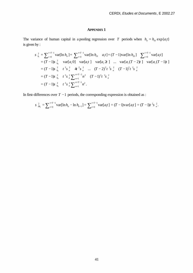
CERDI, Etudes et Documents, E 2002.27
41
APPENDIX 1
The variance of human capital in a pooling regression over T periods when 0 exp{ }it i ih h a t= is given by :
0
0
1 1 120 00 0 0
2
2 2 2 2 2 2 2 2 2 2
var[ln ] var[ln ] ( 1)var[ln ] var[ ]
( 1) var[ 0] var[ ] var[ 2 ] ... var[ ( 2) ] var[ ( 1) ]
( 1) 4 ... ( 2) ( 1)
t
t T t T t Th it i i i it t t
h i i i i i
h a a a
h h a t T h a t
T a a a a T a T
T T T
σ
σ τ τ τ τ
σ τ σ τ σ τ σ τ
= − = − = −
= = == = + = − +
= − + + + + + − + −
= − + + + + − + −
∑ ∑ ∑
0
0
2
22 2 2 2 2 2 21
12 2 2 21
( 1) ( 1)
( 1) .
a
n Th a an
n Th a n
T n T
T n
σ
σ τ σ τ σ
σ τ σ
= −
=
= −
=
= − + + −
= − +
∑∑
In first-differences over 1T − periods, the corresponding expression is obtained as :
1 12 2 210 0
var[ln ln ] var[ ] ( 1)var[ ] ( 1) .t
t T t Th it it i i at t
h h a T a Tσ τ τ τ σ= − = −
∆ −= == − = = − = −∑ ∑
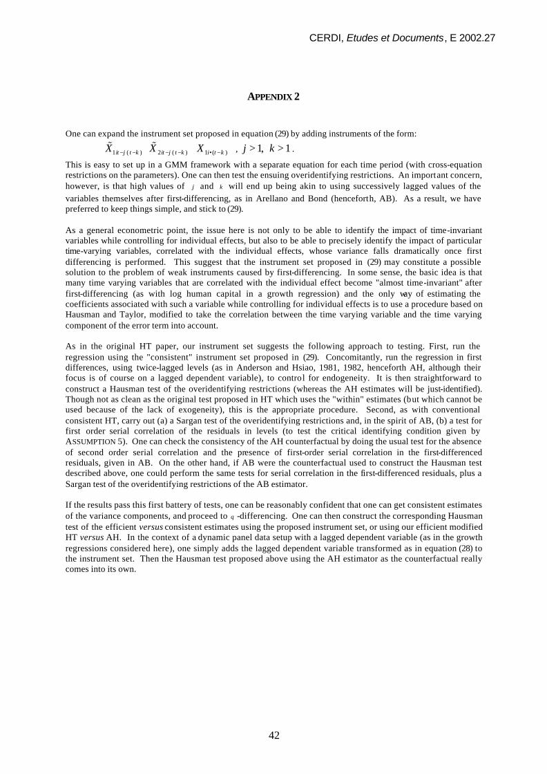
CERDI, Etudes et Documents, E 2002.27
42
APPENDIX 2 One can expand the instrument set proposed in equation (29) by adding instruments of the form:
1 ( ) 2 ( ) 1 ( )it j t k it j t k i t kX X X− − − − • − % % , 1, 1j k> > .
This is easy to set up in a GMM framework with a separate equation for each time period (with cross-equation restrictions on the parameters). One can then test the ensuing overidentifying restrictions. An important concern, however, is that high values of j and k will end up being akin to using successively lagged values of the variables themselves after first-differencing, as in Arellano and Bond (henceforth, AB). As a result, we have preferred to keep things simple, and stick to (29). As a general econometric point, the issue here is not only to be able to identify the impact of time-invariant variables while controlling for individual effects, but also to be able to precisely identify the impact of particular time-varying variables, correlated with the individual effects, whose variance falls dramatically once first differencing is performed. This suggest that the instrument set proposed in (29) may constitute a possible solution to the problem of weak instruments caused by first-differencing. In some sense, the basic idea is that many time varying variables that are correlated with the individual effect become "almost time-invariant" after first-differencing (as with log human capital in a growth regression) and the only way of estimating the coefficients associated with such a variable while controlling for individual effects is to use a procedure based on Hausman and Taylor, modified to take the correlation between the time varying variable and the time varying component of the error term into account. As in the original HT paper, our instrument set suggests the following approach to testing. First, run the regression using the "consistent" instrument set proposed in (29). Concomitantly, run the regression in first differences, using twice-lagged levels (as in Anderson and Hsiao, 1981, 1982, henceforth AH, although their focus is of course on a lagged dependent variable), to control for endogeneity. It is then straightforward to construct a Hausman test of the overidentifying restrictions (whereas the AH estimates will be just-identified). Though not as clean as the original test proposed in HT which uses the "within" estimates (but which cannot be used because of the lack of exogeneity), this is the appropriate procedure. Second, as with conventional consistent HT, carry out (a) a Sargan test of the overidentifying restrictions and, in the spirit of AB, (b) a test for first order serial correlation of the residuals in levels (to test the critical identifying condition given by ASSUMPTION 5). One can check the consistency of the AH counterfactual by doing the usual test for the absence of second order serial correlation and the presence of first-order serial correlation in the first-differenced residuals, given in AB. On the other hand, if AB were the counterfactual used to construct the Hausman test described above, one could perform the same tests for serial correlation in the first-differenced residuals, plus a Sargan test of the overidentifying restrictions of the AB estimator. If the results pass this first battery of tests, one can be reasonably confident that one can get consistent estimates of the variance components, and proceed to θ -differencing. One can then construct the corresponding Hausman test of the efficient versus consistent estimates using the proposed instrument set, or using our efficient modified HT versus AH. In the context of a dynamic panel data setup with a lagged dependent variable (as in the growth regressions considered here), one simply adds the lagged dependent variable transformed as in equation (28) to the instrument set. Then the Hausman test proposed above using the AH estimator as the counterfactual really comes into its own.
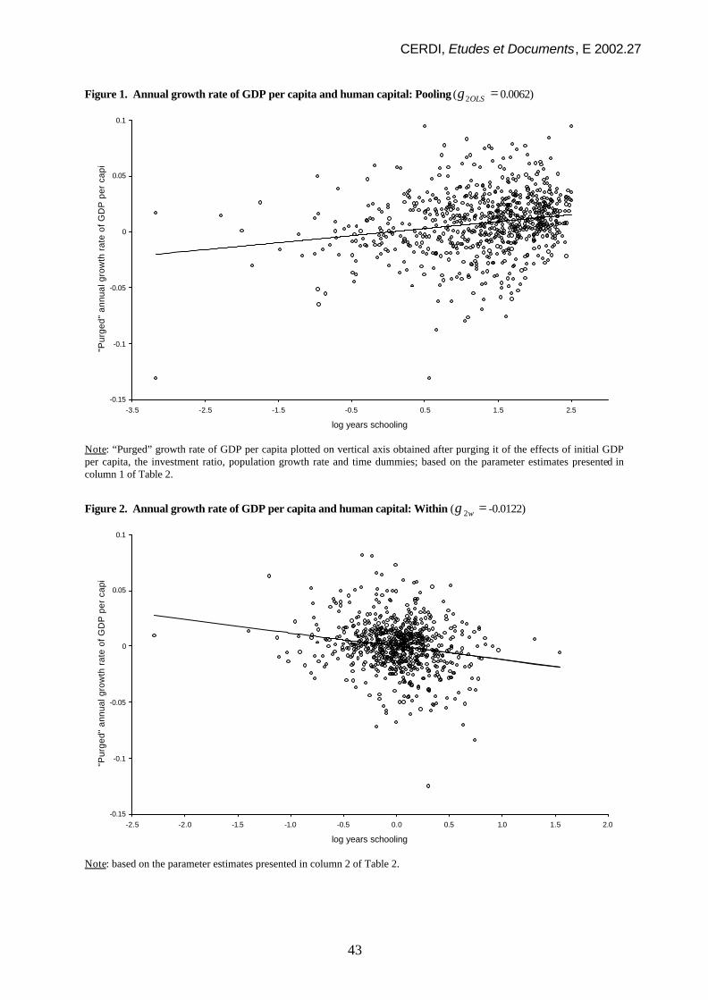
CERDI, Etudes et Documents, E 2002.27
43
Figure 1. Annual growth rate of GDP per capita and human capital: Pooling ( 2OLSγ = 0.0062)
Note: “Purged” growth rate of GDP per capita plotted on vertical axis obtained after purging it of the effects of initial GDP per capita, the investment ratio, population growth rate and time dummies; based on the parameter estimates presented in column 1 of Table 2.
Figure 2. Annual growth rate of GDP per capita and human capital: Within ( 2wγ = -0.0122)
Note: based on the parameter estimates presented in column 2 of Table 2.
-0.15
-0.1
-0.05
0
0.05
0.1
-3.5 -2.5 -1.5 -0.5 0.5 1.5 2.5
log years schooling
"Pur
ged"
ann
ual g
row
th r
ate
of G
DP
per
cap
ita
-0.15
-0.1
-0.05
0
0.05
0.1
-2.5 -2.0 -1.5 -1.0 -0.5 0.0 0.5 1.0 1.5 2.0
log years schooling
"Pur
ged"
ann
ual g
row
th r
ate
of G
DP
per
cap
ita
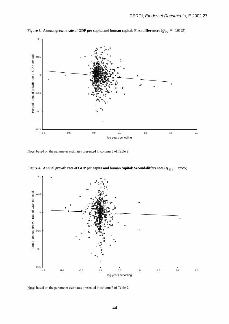
CERDI, Etudes et Documents, E 2002.27
44
Figure 3. Annual growth rate of GDP per capita and human capital: First-differences ( 2dγ = -0.0125)
Note: based on the parameter estimates presented in column 3 of Table 2.
Figure 4. Annual growth rate of GDP per capita and human capital: Second-differences ( 22 dγ = x.xxxx)
Note: based on the parameter estimates presented in column 6 of Table 2.
-0.15
-0.1
-0.05
0
0.05
0.1
-1.0 -0.5 0.0 0.5 1.0 1.5 2.0
log years schooling
"Pur
ged"
ann
ual g
row
th r
ate
of G
DP
per
cap
ita
-0.15
-0.1
-0.05
0
0.05
0.1
-1.5 -1.0 -0.5 0.0 0.5 1.0 1.5 2.0 2.5
log years schooling
"Pur
ged"
ann
ual g
row
th r
ate
of G
DP
per
cap
ita
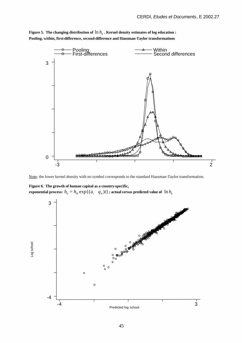
CERDI, Etudes et Documents, E 2002.27
45
Figure 5. The changing distribution of ln ith . Kernel density estimates of log education :
Pooling, within, first-difference, second-difference and Hausman-Taylor transformations
Note: the lower kernel density with no symbol corresponds to the standard Hausman-Taylor transformation. Figure 6. The growth of human capital as a country-specific, exponential process: 0 exp{( ) }it i i ith h a tθ= + ; actual versus predicted value of ln ith
Log
scho
ol
Predicted log school-4 3
-4
3
Pooling Within First-differences Second differences
-3 20
3
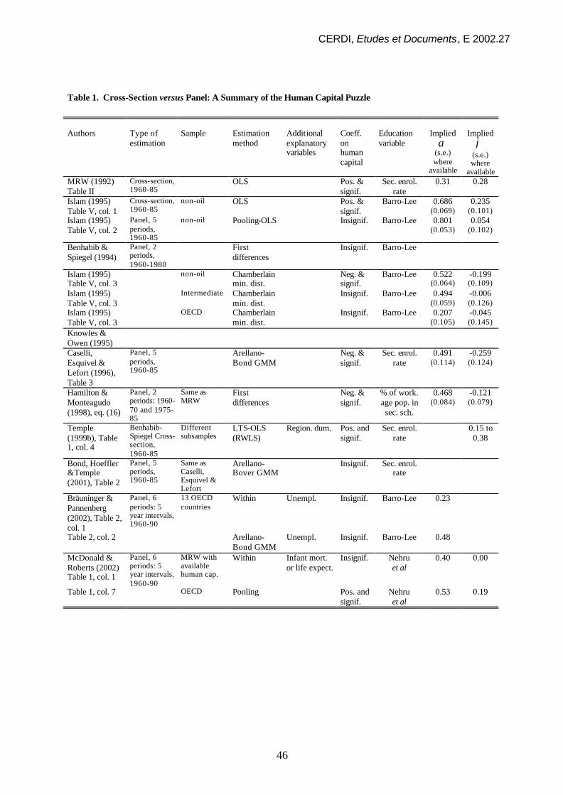
CERDI, Etudes et Documents, E 2002.27
46
Table 1. Cross-Section versus Panel: A Summary of the Human Capital Puzzle Authors
Type of estimation
Sample
Estimation method
Additional explanatory variables
Coeff. on human capital
Education variable
Implied
α (s.e.) where
available
Implied
ϕ (s.e.) where
available MRW (1992) Table II
Cross-section, 1960-85
OLS Pos. & signif.
Sec. enrol. rate
0.31 0.28
Islam (1995) Table V, col. 1
Cross-section, 1960-85
non-oil OLS Pos. & signif.
Barro-Lee 0.686 (0.069)
0.235 (0.101)
Islam (1995) Table V, col. 2
Panel, 5 periods, 1960-85
non-oil Pooling-OLS Insignif. Barro-Lee 0.801 (0.053)
0.054 (0.102)
Benhabib & Spiegel (1994)
Panel, 2 periods, 1960-1980
First differences
Insignif. Barro-Lee
Islam (1995) Table V, col. 3
non-oil Chamberlain min. dist.
Neg. & signif.
Barro-Lee 0.522 (0.064)
-0.199 (0.109)
Islam (1995) Table V, col. 3
Intermediate Chamberlain min. dist.
Insignif. Barro-Lee 0.494 (0.059)
-0.006 (0.126)
Islam (1995) Table V, col. 3
OECD Chamberlain min. dist.
Insignif. Barro-Lee 0.207 (0.105)
-0.045 (0.145)
Knowles & Owen (1995)
Caselli, Esquivel & Lefort (1996), Table 3
Panel, 5 periods, 1960-85
Arellano-Bond GMM
Neg. & signif.
Sec. enrol. rate
0.491 (0.114)
-0.259 (0.124)
Hamilton & Monteagudo (1998), eq. (16)
Panel, 2 periods: 1960-70 and 1975-85
Same as MRW
First differences
Neg. & signif.
% of work. age pop. in sec. sch.
0.468 (0.084)
-0.121 (0.079)
Temple (1999b), Table 1, col. 4
Benhabib-Spiegel Cross-section, 1960-85
Different subsamples
LTS-OLS (RWLS)
Region. dum. Pos. and signif.
Sec. enrol. rate
0.15 to 0.38
Bond, Hoeffler &Temple (2001), Table 2
Panel, 5 periods, 1960-85
Same as Caselli, Esquivel & Lefort
Arellano-Bover GMM
Insignif. Sec. enrol. rate
Bräuninger & Pannenberg (2002), Table 2, col. 1
Panel, 6 periods: 5 year intervals, 1960-90
13 OECD countries
Within Unempl. Insignif. Barro-Lee 0.23
Table 2, col. 2 Arellano-Bond GMM
Unempl. Insignif. Barro-Lee 0.48
McDonald & Roberts (2002) Table 1, col. 1
Panel, 6 periods: 5 year intervals, 1960-90
MRW with available human cap.
Within Infant mort. or life expect.
Insignif. Nehru et al
0.40 0.00
Table 1, col. 7 OECD Pooling Pos. and signif.
Nehru et al
0.53 0.19
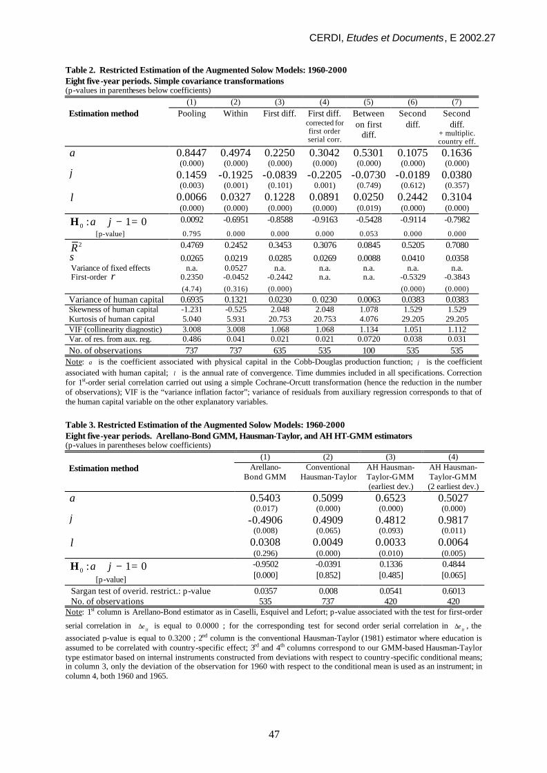
CERDI, Etudes et Documents, E 2002.27
47
Table 2. Restricted Estimation of the Augmented Solow Models: 1960-2000 Eight five -year periods. Simple covariance transformations (p-values in parentheses below coefficients)
(1) (2) (3) (4) (5) (6) (7) Estimation method Pooling Within First diff. First diff.
corrected for first order serial corr.
Between on first
diff.
Second diff.
Second diff.
+ multiplic. country eff.
α 0.8447 0.4974 0.2250 0.3042 0.5301 0.1075 0.1636 (0.000) (0.000) (0.000) (0.000) (0.000) (0.000) (0.000) ϕ 0.1459 -0.1925 -0.0839 -0.2205 -0.0730 -0.0189 0.0380 (0.003) (0.001) (0.101) 0.001) (0.749) (0.612) (0.357)
λ 0.0066 0.0327 0.1228 0.0891 0.0250 0.2442 0.3104 (0.000) (0.000) (0.000) (0.000) (0.019) (0.000) (0.000)
0 : 1 0α ϕ+ − =H 0.0092 -0.6951 -0.8588 -0.9163 -0.5428 -0.9114 -0.7982
[p-value] 0.795 0.000 0.000 0.000 0.053 0.000 0.000 2R 0.4769 0.2452 0.3453 0.3076 0.0845 0.5205 0.7080
σ 0.0265 0.0219 0.0285 0.0269 0.0088 0.0410 0.0358 Variance of fixed effects n.a. 0.0527 n.a. n.a. n.a. n.a. n.a. First-order ρ 0.2350 -0.0452 -0.2442 n.a. n.a. -0.5329 -0.3843 (4.74) (0.316) (0.000) (0.000) (0.000) Variance of human capital 0.6935 0.1321 0.0230 0. 0230 0.0063 0.0383 0.0383 Skewness of human capital -1.231 -0.525 2.048 2.048 1.078 1.529 1.529 Kurtosis of human capital 5.040 5.931 20.753 20.753 4.076 29.205 29.205 VIF (collinearity diagnostic) 3.008 3.008 1.068 1.068 1.134 1.051 1.112 Var. of res. from aux. reg. 0.486 0.041 0.021 0.021 0.0720 0.038 0.031 No. of observations 737 737 635 535 100 535 535
Note: α is the coefficient associated with physical capital in the Cobb-Douglas production function; ϕ is the coefficient associated with human capital; λ is the annual rate of convergence. Time dummies included in all specifications. Correction for 1st-order serial correlation carried out using a simple Cochrane-Orcutt transformation (hence the reduction in the number of observations); VIF is the “variance inflation factor”; variance of residuals from auxiliary regression corresponds to that of the human capital variable on the other explanatory variables. Table 3. Restricted Estimation of the Augmented Solow Models: 1960-2000 Eight five-year periods. Arellano-Bond GMM, Hausman-Taylor, and AH HT-GMM estimators (p-values in parentheses below coefficients)
(1) (2) (3) (4) Estimation method Arellano-
Bond GMM Conventional
Hausman-Taylor AH Hausman-Taylor-GMM (earliest dev.)
AH Hausman-Taylor-GMM (2 earliest dev.)
α 0.5403 0.5099 0.6523 0.5027 (0.017) (0.000) (0.000) (0.000) ϕ -0.4906 0.4909 0.4812 0.9817 (0.008) (0.065) (0.093) (0.011)
λ 0.0308 0.0049 0.0033 0.0064 (0.296) (0.000) (0.010) (0.005)
0 : 1 0α ϕ+ − =H [p-value]
-0.9502 [0.000]
-0.0391 [0.852]
0.1336 [0.485]
0.4844 [0.065]
Sargan test of overid. restrict.: p-value 0.0357 0.008 0.0541 0.6013 No. of observations 535 737 420 420
Note: 1st column is Arellano-Bond estimator as in Caselli, Esquivel and Lefort; p-value associated with the test for first-order
serial correlation in itε∆ is equal to 0.0000 ; for the corresponding test for second order serial correlation in itε∆ , the associated p-value is equal to 0.3200 ; 2nd column is the conventional Hausman-Taylor (1981) estimator where education is assumed to be correlated with country-specific effect; 3rd and 4th columns correspond to our GMM-based Hausman-Taylor type estimator based on internal instruments constructed from deviations with respect to country-specific conditional means; in column 3, only the deviation of the observation for 1960 with respect to the conditional mean is used as an instrument; in column 4, both 1960 and 1965.


![MOSFETs [CHAPTER 6]apachepersonal.miun.se/~gorthu/device/Omi.pdfmicrowave amplifiers •Higher input impedance than bipolar transistors •Thermally stable Negative temperature coefficient](https://img.pdfslide.us/doc/110x75/5e3a4e73b69ac32a5040b7b5/mosfets-chapter-6-gorthudeviceomipdf-microwave-amplifiers-ahigher-input-impedance.jpg)