FEDERAL RESERVE BANK OF SAN FRANCISCO

WORKING PAPER SERIES

Explaining Exchange Rate Anomalies in a Model with Taylor-rule Fundamentals and Consistent Expectations

Kevin J. Lansing Federal Reserve Bank of San Francisco

Jun Ma

University of Alabama

June 2016

Working Paper 2014-22

http://www.frbsf.org/economic-research/publications/working-papers/wp2014-22.pdf

Suggested citation:

Lansing, Kevin J., Jun Ma. 2016. “Explaining Exchange Rate Anomalies in a Model with Taylor-rule Fundamentals and Consistent Expectations.” Federal Reserve Bank of San Francisco Working Paper 2014-22. http://www.frbsf.org/economic-research/publications/working-papers/wp2014-22.pdf The views in this paper are solely the responsibility of the authors and should not be interpreted as reflecting the views of the Federal Reserve Bank of San Francisco or the Board of Governors of the Federal Reserve System.

Explaining Exchange Rate Anomalies in a Model withTaylor-rule Fundamentals and Consistent Expectations

June 27, 2016

Abstract

We introduce boundedly-rational expectations into a standard asset-pricing model ofthe exchange rate, where cross-country interest rate di¤erentials are governed by Taylor-type rules. Agents augment a lagged-information random walk forecast with a term thatcaptures news about Taylor-rule fundamentals. The coe¢ cient on fundamental news ispinned down using the moments of observable data such that the resulting forecast errorsare close to white noise. The model generates volatility and persistence that is remarkablysimilar to that observed in monthly exchange rate data for Canada, Japan, and the U.K.Regressions performed on model-generated data can deliver the well-documented forwardpremium anomaly.

Keywords: Exchange rates, Uncovered interest rate parity, Forward premium anomaly,Random-walk expectations, Excess volatility.

JEL Classi�cation: D83, D84, E44, F31, G17.

1 Introduction

This paper develops a simple framework that can reproduce numerous quantitative features

of real-world exchange rates. The key aspect of our approach is the way in which agents�

expectations are modeled. Starting from a standard asset-pricing model of the exchange

rate, we postulate that agents augment a lagged-information random walk forecast with news

about fundamentals. Fundamentals in our model are determined by cross-country interest

rate di¤erentials which, in turn, are described by Taylor-type rules, along the lines of Engel

and West (2005, 2006). We solve for a �consistent expectations equilibrium,� in which the

coe¢ cient on fundamental news in the agent�s subjective forecast rule is pinned down using

the observed covariance between exchange rate changes and fundamental news. This learnable

equilibrium delivers the result that the forecast errors observed by an agent are close to white

noise, making it di¢ cult to detect any misspeci�cation of the subjective forecast rule.1

We demonstrate that our consistent expectations model can generate volatility and per-

sistence that is remarkably similar to that observed in monthly bilateral exchange rate data

(relative to the U.S.) for Canada, Japan, and the U.K. over the period 1974 to 2012. We

show that regressions performed on model-generated data can deliver the so-called �forward-

premium anomaly,�whereby a high interest rate currency tends to appreciate, thus violating

the uncovered interest parity (UIP) condition. Moreover, the estimated slope coe¢ cient in

the model UIP regressions can vary over a wide range when estimated using a rolling sample

period. This result is consistent with the wide range of coe¢ cient estimates observed across

countries and time periods in the data.2

In our model, agents�perceived law of motion (PLM) for the exchange rate is a driftless

random walk that is modi�ed to include an additional term involving fundamental news,

i.e., the innovation to the AR(1) driving process that is implied by the Taylor-rule based

interest rate di¤erential. The standard asset-pricing model implies that the contemporaneous

realization of the exchange rate at time t depends in part on agents�subjective forecast of the

exchange rate at time t+1: Following the methodology of the adaptive learning literature, we

postulate that when constructing their subjective forecast, agents employ the lagged realization

of the exchange rate at time t � 1: Use of the lagged realization ensures that the forecast is�operational.�Since the contemporaneous realization depends on the forecast, it is not clear

how agents could make use of this realization when constructing their forecast in real-time.

Our setup captures an idea originally put forth in an informal way by Froot and Thaler (1990),

who suggested that the empirical failure of the UIP condition might be linked to the fact that

1The equilibrium concept that we employ was originally put forth by Hommes and Sorger (1998). A closely-related concept is the �restricted perceptions equilibrium�described by Evans and Honkopohja (2001, Chapter13). For other applications of consistent expectations to asset pricing or in�ation, see Sögner and Mitlöhner(2002), Branch and McGough (2005), Evans and Ramey (2006), Lansing (2009, 2010), and Hommes and Zhu(2014).

2For evidence of variability in estimated UIP slope coe¢ cients, see Bansal (1997), Flood and Rose (2002),Baillie and Chang (2011), Baillie and Cho (2014), and Ding and Ma (2013).

1

investors �may need some time to think about trades before executing them, or that they

simply cannot respond quickly to recent information.�

We assume that enough time has gone by for agents to have discovered the parameters

governing the law of motion for the fundamental driving variable, thus allowing them to

infer the fundamental innovation, i.e., news. Given the time series of past data, agents�can

estimate the coe¢ cient on fundamental news in their PLM by running a simple regression.

The agents�forecast rule can be viewed as boundedly-rational because the resulting actual law

of motion (ALM) for the exchange rate exhibits a near-unit root with innovations that depend

on Taylor-rule fundamentals.3

We show that regardless of the starting value for the coe¢ cient on fundamental news in the

subjective forecast rule, a standard real-time learning algorithm will converge to the vicinity

of the �xed point which de�nes the unique consistent expectations (CE) equilibrium. Use

of the lagged exchange rate in the subjective forecast rule is the crucial element needed to

generate the forward-premium anomaly. In equilibrium, the CE model delivers substantial

�excess volatility�of the exchange rate relative to the rational expectations (RE) version of

the model. Indeed, the CE model�s prediction for the volatility of exchange rate changes is

very close to that observed in the data.

Our setup is motivated by two important features of the data: (1) real-world exchange

rates exhibit near-random walk behavior, and (2) exchange rates and fundamentals do exhibit

some tenuous empirical links. Andersen et al. (2003) employ high frequency data to show

that fundamental macroeconomic news surprises induce shifts in the exchange rate. Survey

responses from professional exchange rate forecasters indicate that the vast majority use fun-

damental economic data to help construct their forecasts (Dick and Menkho¤ 2013; Ter Ellen

et al. 2013).

When we apply the CE model�s forecast rule to exchange rate data for Canada, Japan, and

the U.K., we �nd that the inclusion of fundamental news together with the lagged exchange rate

helps to improve forecast accuracy relative to an otherwise similar random walk forecast that

omits the fundamental news term. Moreover, once the fundamental news term is included in

the forecasting regression, forecast performance is often improved by using the lagged exchange

rate rather than the contemporaneous exchange rate.

Using survey data of �nancial institutions for 3-month ahead forecasts of exchange rates,

we show that changes in the interest rate di¤erential (a proxy for fundamental news) are helpful

in explaining movements in the survey forecasts� a result that is consistent with the subjective

forecast rule in the CE model. In particular, the data show that survey respondents tend to

forecast a currency appreciation during periods when the change of interest rate di¤erential is

positive.

3Lansing (2010) employs a similar random walk plus fundamentals subjective forecast rule in a standardLucas-type asset pricing model to account for numerous quantitative features of long-run U.S. stock marketdata.

2

1.1 Related Literature

E¤orts to explain movements in exchange rates as a rational response to economic funda-

mentals have, for the most part, met with little success. More than thirty years ago, Meese

and Rogo¤ (1983) demonstrated that none of the usual economic variables (money supplies,

real incomes, trade balances, in�ation rates, interest rates, etc.) could help forecast future

exchange rates better than a simple random walk forecast. With three decades of additional

data in hand, researchers continue to con�rm the Meese-Rogo¤ results.4 While some tenuous

links between fundamentals and exchange rates have been detected, the empirical relationships

are generally unstable (Bacchetta and Van Wincoop 2004, 2013), hold only at 5 to 10 year

horizons (Chinn 2006), or operate in the wrong direction, i.e., exchange rates may help predict

fundamentals but not vice versa (Engel and West 2005).5 The failure of traditional funda-

mental variables to improve forecasts of future exchange rates has been called the �exchange

rate disconnect puzzle.�

Another puzzle relates to the �excess volatility�of exchange rates. Like stock prices, ex-

change rates appear to move too much when compared to changes in observable fundamentals.6

Engel and West (2006) show that a standard rational expectations model can match the ob-

served persistence of real-world exchange rates, but it substantially underpredicts the observed

volatility. West (1987) makes the point that exchange rate volatility can be reconciled with

fundamental exchange rate models if one allows for �regression disturbances,�i.e., exogenous

shocks that can be interpreted as capturing shifts in unobserved fundamentals. Similarly,

Balke et al. (2013) �nd that unobserved factors (labeled �money demand shifters�) account

for most of the volatility in the U.K./U.S. exchange rate using data that extends back more

than a century. An innovative study by Bartolini and Gioginianni (2001) seeks to account for

the in�uence of unobserved fundamentals using survey data on exchange rate expectations.

The study �nds �broad evidence...of excess volatility with respect to the predictions of the

canonical asset-pricing model of the exchange rate with rational expectations�(p. 518).

A third exchange rate puzzle is the so-called �forward-premium anomaly.� In theory, a

currency traded at a premium in the forward market predicts a subsequent appreciation of

that currency in the spot market. In practice, there is a close empirical link between the

observed forward premium and cross-country interest rate di¤erentials, consistent with the

covered interest parity condition. Hence, theory predicts that a low interest rate currency

should, on average, appreciate relative to a high interest rate currency because the subsequent

appreciation compensates investors for the opportunity cost of holding a low interest rate

4The Meese-Rogo¤ results are very robust; they show that realized future fundamentals also fail to forecastfuture exchange rates. For surveys of this vast literature, see Rossi (2013), Cheung, Chinn and Pascual (2005),and Sarno (2005).

5Speci�cally, Engel and West (2005) �nd Granger causality running from exchange rates to fundamentals.Recently, however, Ko and Ogaki (2015) demonstrate that this result is not robust after correcting for thesmall-sample size.

6Early studies applied to exchange rate volatility include Huang (1981) and Wadhwani (1987).

3

bond. The theoretical slope coe¢ cient from a regression of the observed exchange rate change

on the prior interest rate di¤erential is exactly equal to one. This prediction of the theory,

known as the uncovered interest parity condition, is grossly violated in the data. Regressions

of the observed exchange rate change on the prior interest rate di¤erential yield estimated

slope coe¢ cients that are typically negative and signi�cantly di¤erent from one (Fama 1984).

Like the other two puzzles, the forward-premium anomaly has stood the test of time.7

The wrong sign of the slope coe¢ cient in UIP regressions can be reconciled with no-

arbitrage and rational expectations if investors demand a particular type of risk premium to

compensate for holding an uncovered currency position. By failing to account for a potentially

time-varying risk premium that may co-move with the interest rate di¤erential, the standard

UIP regression may deliver a biased estimate of the slope coe¢ cient.8 Lustig and Verdelhan

(2007) provide some evidence that carry-trade pro�ts (excess returns from betting against UIP)

may re�ect a compensation for risk that stems from a negative correlation between the carry-

trade pro�ts and investors�consumption-based marginal utility.9 However, Burnside (2011)

points out that their empirical model is subject to weak identi�cation such that there is no

concrete evidence for the postulated connection between carry-trade pro�ts and fundamental

risk. Moreover, Burnside et al. (2011) show that there is no statistically signi�cant covariance

between carry-trade pro�ts and conventional risk factors.

Verdelhan (2010) develops a rational model with time-varying risk premiums along the

lines of Campbell and Cochrane (1999). The model implies that rational domestic investors

will expect low future returns on risky foreign bonds in good times (due to an expected

appreciation of the domestic currency) when risk premia are low and domestic interest rates

are high relative to foreign interest rates. Hence, the model delivers the prediction that the

domestic currency will appreciate, on average, when domestic interest rates are high� thus

violating the UIP condition, as in the data. Unfortunately, the idea that investors expect low

future returns in good times is strongly contradicted by a wide variety of survey evidence. The

survey evidence shows that investors typically expect high future returns in good times, as

they extrapolate from past return data.10 Overall, the survey evidence tells us that rationally

time-varying risk premiums are not a convincing explanation for the empirical failure of UIP.

Our approach relates to some previous literature that has employed models with distorted

beliefs to account for the behavior of exchange rates. Gourinchas and Tornell (2004) postulate

that agents have distorted beliefs about the law of motion for fundamentals. Related mech-

anisms are proposed by Burnside et al. (2011), Ilut (2012), and Yu (2013). In contrast, we

postulate that agents have distorted beliefs about the law of motion for exchange rates, not

7For recent evidence, see Baillie and Chang (2011) and Baillie and Cho (2014).8See Engel (1996) for a survey of this large literature and Engel (2014) for a review of new developments in

this �eld.9See also Lustig et al. (2014).10For additional details, see Amromin and Sharpe (2014), Greenwood and Shleifer (2014), and Koijen et al.

(2015).

4

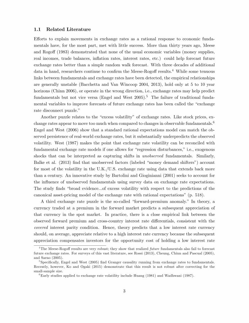
Figure 1: There is no tight systematic relationship between monthly exchange rate changes andthe prior month�s interest rate di¤erential (exchange rate disconnect puzzle). The slope of the �ttedrelationship between the observed exchange rate change and the prior month�s interest rate di¤erentialis negative (forward-premium anomaly).

fundamentals.

Bacchetta and Van Wincoop (2007) introduce �random walk expectations� into an ex-

change rate model with risk aversion and infrequent portfolio adjustments. Unlike our setup,

the agent�s subjective forecast in their model completely ignores fundamentals. While their

model can account for the forward-premium anomaly, it relies on exogenous shocks from ad

hoc noise traders to account for the observed volatility of exchange rate changes.

Chakraborty and Evans (2008) introduce constant-gain learning about the reduced-form

law of motion for the exchange rate. The agent in their model employs the correct (i.e., ra-

tional) form for the law of motion, but the estimated parameters are perpetually updated

using recent data. They show that statistical variation in the estimated parameters may

cause the UIP condition to be violated, particularly in small samples. However, their model

does not account for excess volatility of the exchange rate. Mark (2009) develops a model

with perpetual learning about the Taylor-rule coe¢ cients that govern the cross-country in-

terest rate di¤erential. He shows that the model can account for major swings in the real

deutschemark/euro-dollar exchange rate over the period 1976 to 2007.

5

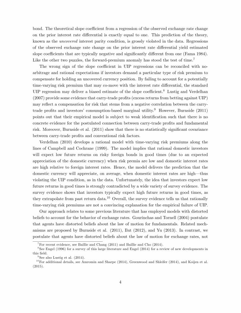
Figure 2: The volatility of the exchange rate change is 10 to 40 times higher than the volatility of thecross-country interest rate di¤erential (excess volatility puzzle). Estimated UIP slope coe¢ cients liemostly in negative territory and exhibit substantial time variation.

2 Exchange Rate Anomalies

According to UIP theory, the cross-country interest rate di¤erential should be a key ex-

planatory variable for subsequent exchange rate changes. Figure 1 plots scatter diagrams

of monthly bilateral exchange rate changes (in annualized percent) versus the prior month�s

average short-term nominal interest rate di¤erential (in percent) for three pairs of countries,

namely, Canada/U.S., Japan/U.S. and U.K./U.S. The data covers the period from January

1974 through October 2012.11 The bottom right panel of Figure 1 shows a scatter diagram of

the pooled data.

Figure 1 shows that there is no tight systematic relationship between monthly exchange

rate changes and the prior month�s interest rate di¤erential (exchange rate disconnect puzzle).

The dashed regression lines in Figure 1 show a negative slope in the �tted relationship between

the observed exchange rate change and the prior month�s interest rate di¤erential (forward-

premium anomaly). The top left panel of Figure 2 plots the relative volatility of exchange rate

changes to interest rate di¤erentials, where volatilities are computed as the standard deviation

11Exchange rate changes are computed as the log di¤erence of sequential end-of-month values and thenannualized. Interest rates are annualized 3-month government bond yields. All data are from the IMF�sInternational Financial Statistics database.

6

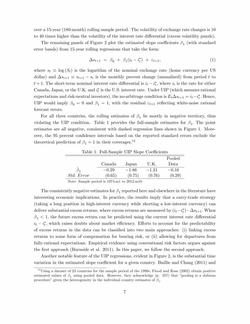
over a 15-year (180-month) rolling sample period. The volatility of exchange rate changes is 10

to 40 times higher than the volatility of the interest rate di¤erential (excess volatility puzzle).

The remaining panels of Figure 2 plot the estimated slope coe¢ cients �1 (with standard

error bands) from 15-year rolling regressions that take the form:

�st+1 = �0 + �1(it � i�t ) + "t+1; (1)

where st � log (St) is the logarithm of the nominal exchange rate (home currency per US

dollar) and �st+1 � st+1 � st is the monthly percent change (annualized) from period t to

t+1: The short-term nominal interest rate di¤erential is it� i�t , where it is the rate for eitherCanada, Japan, or the U.K. and i�t is the U.S. interest rate. Under UIP (which assumes rational

expectations and risk-neutral investors), the no-arbitrage condition is Et�st+1 = it�i�t : Hence,UIP would imply �0 = 0 and �1 = 1; with the residual "t+1 re�ecting white-noise rational

forecast errors.

For all three countries, the rolling estimates of �1 lie mostly in negative territory, thus

violating the UIP condition. Table 1 provides the full-sample estimates for �1: The point

estimates are all negative, consistent with dashed regression lines shown in Figure 1. More-

over, the 95 percent con�dence intervals based on the reported standard errors exclude the

theoretical prediction of �1 = 1 in their coverages.12

Table 1. Full-Sample UIP Slope Coe¢ cients

Canada Japan U.K.PooledData

�̂1 �0:29 �1:86 �1:21 �0:16Std: Error (0.65) (0.75) (0.76) (0.29)Note: Sample period is 1974.m1 to 2012.m10.

The consistently negative estimates for �1 reported here and elsewhere in the literature have

interesting economic implications. In practice, the results imply that a carry-trade strategy

(taking a long position in high-interest currency while shorting a low-interest currency) can

deliver substantial excess returns, where excess returns are measured by (it�i�t )��st+1:When�1 < 1; the future excess return can be predicted using the current interest rate di¤erential

it � i�t ; which raises doubts about market e¢ ciency. E¤orts to account for the predictabilityof excess returns in the data can be classi�ed into two main approaches: (i) linking excess

returns to some form of compensation for bearing risk, or (ii) allowing for departures from

fully-rational expectations. Empirical evidence using conventional risk factors argues against

the �rst approach (Burnside et al. 2011). In this paper, we follow the second approach.

Another notable feature of the UIP regressions, evident in Figure 2, is the substantial time

variation in the estimated slope coe¢ cient for a given country. Baillie and Chang (2011) and

12Using a dataset of 23 countries for the sample period of the 1990s, Flood and Rose (2002) obtain positiveestimated values of �1 using pooled data. However, they acknowledge (p. 257) that �pooling is a dubiousprocedure�given the heterogeneity in the individual country estimates of �1:

7

Baillie and Cho (2014) employ time-varying parameter regressions to capture this feature of

the data. Bansal (1997) shows that the sign of �1 appears to be correlated with the sign

of the interest rate di¤erential, but his results do not generalize to other sample periods

or countries. Ding and Ma (2013) develop a model of cross-border portfolio reallocation

that can help explain a time-varying �1 estimate. Our model can deliver a negative and

statistically signi�cant estimate of �1 in long-sample regressions as well as substantial time-

variation in the estimated slope coe¢ cient in rolling regressions. The time variation in the

estimated slope coe¢ cient arises for two reasons: (i) the actual law of motion that governs

�st+1 in the consistent expectations equilibrium turns out to di¤er in signi�cant ways from

the UIP regression equation (1), and (ii) the volatility of �st+1 in the consistent expectations

equilibrium is much higher than the volatility of it � i�t :

3 Model

The framework for our analysis is a standard asset-pricing model of the exchange rate. Funda-

mentals are given by cross-country interest rate di¤erentials which, in turn, are described by

Taylor-type rules. Given our data, the home country in the model represents either Canada,

Japan, or the U.K. while the foreign country represents the United States (denoted by �variables).

We postulate that the home country central bank sets the short-term nominal interest rate

according to the following Taylor-type rule

it = �it�1 + (1� �)f g��t + gyyt + gs[st � �st�1 � (1� �)st]g + �t; (2)

where it is the short term nominal interest rate, �t is the in�ation rate (log di¤erence of the

price level over the past 12 months), yt is the output gap (log deviation of actual output from

potential output), st is the log of the nominal exchange rate (home currency per U.S. dollar),

st�1 is the lagged exchange rate, and st � pt�p�t is a benchmark exchange rate implied by thepurchasing power parity (PPP) condition, where pt is the domestic price level and p�t is the

foreign price level.13 When � = 0; the central bank reacts to st � st which is the deviation ofthe exchange rate from the PPP benchmark, consistent with the models employed by Engel

and West (2005, 2006). When � = 1; the central bank reacts to the exchange rate change

�st = st � st�1; consistent with the empirical policy rule estimates of Lubik and Schorfheide(2007) and Justiniano and Preston (2010) for a variety of industrial countries. Motivated by

the empirical evidence, we set � ' 1.14 The term �t represents an exogenous monetary policy

shock. In contrast to Engel and West (2005, 2006), we allow for interest-rate smoothing on

the part of the central bank, as governed by the parameter � > 0: For the remaining reaction13We omit constant terms from equation (2) because our empirical application of the central bank reaction

function makes use of demeaned data.14As noted below, we impose the parameter restriction 0 � � < 1 to ensure the existence of a unique rational

expectations solution of the model.

8

function parameters, we follow standard practice in assuming g� > 1; and gy; gs > 0: In other

words, the central bank responds more than one-for-one to movements in in�ation and raises

the nominal interest rate in response to a larger output gap or a depreciating home currency

(�st > 0).

The foreign (i.e., U.S.) central bank sets the short-term nominal interest rate according to

i�t = �i�t�1 + (1� �)[ g���t + gyy�t ] + ��t ; (3)

where we assume that the reaction function parameters �; g�; and gy are the same across

countries.15 Subtracting equation (3) from equation (2) yields the following expression for the

cross-country interest rate di¤erential

it � i�t = �(it�1 � i�t�1) + (1� �) f g�(�t � ��t ) + gy(yt � y�t ) + gs [st � �st�1 � (1� �)st] g+ �t � ��t : (4)

Assuming risk-neutral, rational investors, the uncovered interest rate parity condition im-

plies

Etst+1 � st = it � i�t ; (5)

where Etst+1 is the rational forecast of next period�s log exchange rate.16 The UIP condition

says that a negative interest rate di¤erential it�i�t < 0 will exist when rational investors expecta home currency appreciation, i.e., when Etst+1 < st: The expected appreciation compensates

investors for the opportunity cost of holding a low interest rate domestic bond rather than

a high interest rate foreign bond. Rational expectations implies Etst+1 = st+1 � "t+1, where"t+1 is a white-noise forecast error. Hence, theory predicts that, on average, a low interest rate

currency should appreciate relative to a high interest rate currency such that E (st+1 � st) < 0:Substituting the cross-country interest rate di¤erential (4) into the UIP condition (5)

and solving for st yields the following no-arbitrage condition that determines the equilibrium

exchange rate

st = bEtst+1 + �(1� b)st�1 + xt; b � 1

1 + (1� �)gs< 1; (6)

where b is the e¤ective discount factor and xt is the fundamental driving variable de�ned as

xt � �b�(it�1�i�t�1) � b(1��)[ g�(�t���t )+gy(yt�y�t )�gs(1��)(pt�p�t )] � b (�t � ��t ) ; (7)

where we have made the substitution st = pt � p�t .17

15Consistent with the literature (see for example Engel and West 2005) we assume that the U.S. policyinterest rate does not react to the exchange rate. For convenience, we assume that the remaining policy ruleparameters are the same across countries. A departure from either of these assumptions would not alter themodel or the quantitative results in a substantial way. See footnote 17 for further clari�cation.16More precisely, the UIP condition is EtSt+1=St = (1 + it) = (1 + i�t ) : Following standard practice, we take

logs of both sides and ignore the Jensen�s inequality term such that log (EtSt+1) ' Et log (St+1) :17The basic form of equations (6) and (7) will remain unchanged if we assume that the foreign central bank

also reacts to the exchange rate, but with a smaller reaction coe¢ cient g�s < gs: In this case, the e¤ectivediscount factor becomes b = 1= [1 + (1� �) (gs � g�s )] :

9

The no-arbitrage condition (6) shows that the equilibrium exchange rate st depends on

the agent�s conditional forecast Etst+1; the lagged exchange rate st�1, and the fundamental

driving variable xt. When 0 � � < 1; the sum of the coe¢ cients on Etst+1 and st�1 is less

than one which ensures the existence of a unique rational expectations solution. The general

form of equation (6), whereby the current value of an endogenous variable depends on its own

expected future value, its lagged value, and a driving variable appears in a wide variety of

economic models, such as the hybrid New Keynesian Phillips Curve (Galí, et al. 2005).

The macroeconomic variables that enter the de�nition of xt exhibit a high degree of persis-

tence in the data. We therefore model the behavior of the fundamental driving variable using

the following stationary AR(1) process

xt = �xt�1 + ut; ut � N�0; �2u

�; j�j < 1; (8)

where the parameter � governs the degree of persistence. While some studies allow for a

unit root in the law of motion for fundamentals, we maintain the assumption of stationarity

for consistency with most of the literature. In a �nite data sample, it is nearly impossible

to distinguish between a unit root process and one that is stationary but highly persistent

(Cochrane 1991).

Given values for xt and st; we can recover the current-period interest rate di¤erential as

follows

it � i�t = �1bxt +

�1� bb

�(st � �st�1) : (9)

Empirical estimates of central bank policy rules typically imply � values in the range of 0.8 to

0.9 together with small values for gs such that b ' 1: In this case, the equilibrium dynamics

for it � i�t will be very similar to the equilibrium dynamics for �xt: We will make use of thisinverse relationship between the interest rate di¤erential and the fundamental driving variable

in our discussion of the results.

Our description of monetary policy in terms of Taylor-type interest rate rules has solid em-

pirical support using data for many countries from the 1980�s onwards (Lubik and Schorfheide

2007, Justiniano and Preston 2010). But even for earlier sample periods when Taylor-type

rules may not have been followed, there would still exist a general feedback mechanism that

implies some type of monetary policy response (e.g., a shift in the money growth rate) to

movements in the exchange rate in order to help stabilize the macro-economy. For exam-

ple, given a speci�cation for money demand, a shift of the money growth rate in response to

a movement in the exchange rate could be mapped to a corresponding shift in the interest

rate di¤erential. The Taylor-type interest rate rules (2) and (3) capture the idea of feedback

mechanism from exchange rates to monetary policy in a tractable way, allowing us to com-

pare the predictions of our consistent expectations model to an otherwise similar model with

fully-rational expectations.

10

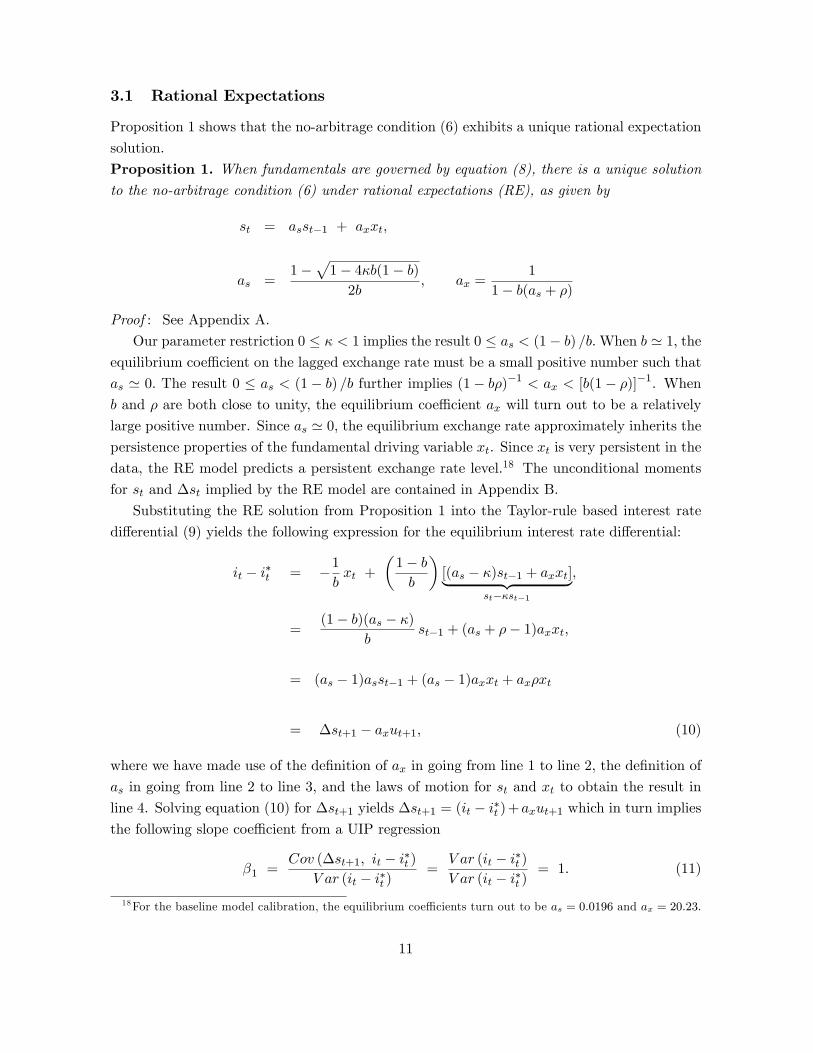
3.1 Rational Expectations

Proposition 1 shows that the no-arbitrage condition (6) exhibits a unique rational expectation

solution.

Proposition 1. When fundamentals are governed by equation (8), there is a unique solutionto the no-arbitrage condition (6) under rational expectations (RE), as given by

st = asst�1 + axxt;

as =1�

p1� 4�b(1� b)2b

; ax =1

1� b(as + �)

Proof : See Appendix A.

Our parameter restriction 0 � � < 1 implies the result 0 � as < (1� b) =b:When b ' 1; theequilibrium coe¢ cient on the lagged exchange rate must be a small positive number such that

as ' 0: The result 0 � as < (1� b) =b further implies (1� b�)�1 < ax < [b(1� �)]�1. Whenb and � are both close to unity, the equilibrium coe¢ cient ax will turn out to be a relatively

large positive number. Since as ' 0; the equilibrium exchange rate approximately inherits the

persistence properties of the fundamental driving variable xt. Since xt is very persistent in the

data, the RE model predicts a persistent exchange rate level.18 The unconditional moments

for st and �st implied by the RE model are contained in Appendix B.

Substituting the RE solution from Proposition 1 into the Taylor-rule based interest rate

di¤erential (9) yields the following expression for the equilibrium interest rate di¤erential:

it � i�t = �1bxt +

�1� bb

�[(as � �)st�1 + axxt]| {z }

st��st�1

;

=(1� b)(as � �)

bst�1 + (as + �� 1)axxt;

= (as � 1)asst�1 + (as � 1)axxt + ax�xt

= �st+1 � axut+1; (10)

where we have made use of the de�nition of ax in going from line 1 to line 2, the de�nition of

as in going from line 2 to line 3, and the laws of motion for st and xt to obtain the result in

line 4. Solving equation (10) for �st+1 yields �st+1 = (it � i�t )+axut+1 which in turn impliesthe following slope coe¢ cient from a UIP regression

�1 =Cov (�st+1; it � i�t )

V ar (it � i�t )=V ar (it � i�t )V ar (it � i�t )

= 1: (11)

18For the baseline model calibration, the equilibrium coe¢ cients turn out to be as = 0:0196 and ax = 20:23:

11

3.2 Consistent Expectations

Real-world exchange rates exhibit near-random walk behavior. A naive forecast rule that uses

only the most recently-observed exchange rate almost always outperforms a fundamentals-

based forecast (Rossi 2013). In addition to its predictive accuracy, a random walk forecast has

the advantage of economizing on computational and informational resources. As described

many years ago by Nerlove (1983), �Purposeful economic agents have incentives to eliminate

errors up to a point justi�ed by the costs of obtaining the information necessary to do so...The

most readily available and least costly information about the future value of a variable is its

past value�(p. 1255).

Despite the dominance of a random walk forecast, survey evidence indicates that market

participants continue to pay attention to fundamentals. A recent study by Dick and Menkho¤

(2013) uses survey data to analyze the methods of nearly 400 professional exchange rate

forecasters. The data shows that the vast majority of forecasters employ fundamental economic

data together with past exchange rate movements to help construct their forecasts. Another

study of survey data by Ter Ellen et al. (2014) �nds evidence that large wholesale investors in

the foreign exchange market employ fundamentals-based strategies as part of their forecasting

toolkit.

To capture the above ideas, we postulate that agents�perceived law of motion (PLM) for

the exchange rate is given by

st = st�1 + �ut; (12)

where ut represents �fundamental news,� as measured by the innovation to the AR(1) fun-

damental driving process (8). A long history of observations of xt would allow the agent to

discover the law of motion for fundamentals and infer the value of ut from sequential obser-

vations of xt and xt�1: Given the past data, agents could estimate the value of the parameter

� by running a regression of �st on ut: When � 6= 0; the PLM implies that a fundamental

news shock will induce an immediate jump in the exchange rate, consistent with the �ndings

of Andersen et al. (2003) who employ high frequency data.

The PLM is used by agents to construct a subjective forecast bEt st+1 which takes theplace of the rational forecast Et st+1 in the no-arbitrage condition (6). Following Yu (2013),

p. 476, our solution procedure assumes that the no-arbitrage condition �holds ex ante under

investors�perception.�19 But ex post, the exchange rate evolves according to the actual law of

motion (ALM) to be derived below. Since the no-arbitrage condition implies that st depends

in part on the subjective forecast, it is not clear how an agent could make use of st when

constructing a forecast in real-time. Even in high frequency trading environments, investors

who submit market orders to buy or sell an asset do not know the exact price at which their

order will be �lled. To deal with this timing issue, models that employ adaptive learning or

other forms of boundedly-rational expectations typically assume that agents can only make

19This is also the setup in the distorted-belief models of Gourinchas and Tornell (2004) and Ilut (2012).

12

use of the lagged realization of the forecast variable (in this case st�1) when constructing their

subjective forecast at time t.20 According to the de�nition (7), xt does not not depend on stso there is no controversy about including it in agents�information at time t:

Our lagged-information setup can be viewed as a reduced-form way of capturing various

types of information frictions. The �sticky information�model of Mankiw and Reis (2002)

postulates that only a fraction of agents update to the current vintage rational forecast each

period. A �noisy information�model along the lines of Coibion and Gordonichencko (2015)

implies that the current vintage rational forecast itself is a moving average of past observed

values. Combining these two frictions could result in a very small weight assigned to the

most recent data observation in the aggregate market forecast. Later, we show that forecast

accuracy in the data can often be improved by using st�1 rather than st in rolling forecast

regressions that include a fundamental news term.21

Since the agent employs lagged information about the exchange rate, the PLM (12) is

iterated ahead two periods to obtain their subjective forecast

bE t st+1 = bE t [st + �ut+1] ;= bE t [st�1 + �ut + �ut+1] ;= st�1 + �ut; (13)

which makes use of the lagged exchange rate st�1, together with the contemporaneous funda-

mental news shock.

Substituting the agent�s subjective forecast (13) into the no-arbitrage condition (6) and

solving for st yields the following actual law of motion for the exchange rate

st = [1� (1� �)(1� b)] st�1 + b�ut + xt; (14)

where xt is governed by (8). Notice that the form of the ALM is similar, but not identical,

to the RE model solution from Proposition 1. Recall that we previously showed that the

equilibrium coe¢ cient on the lagged exchange rate in the RE model must be a small positive

number such that as ' 0: In the CE model, the parameter restriction 0 � � < 1 implies thatthe equilibrium coe¢ cient on the lagged exchange rate has a lower bound of b when � = 0:

This lower bound is close to unity when b ' 1: Since the equilibrium coe¢ cient on st�1 in the

CE model is near unity, the agents�perception of a unit root in the exchange rate turns out to

be close to self-ful�lling. Hence we can say that agents are forecasting in a way that appears

near-rational.20For an overview of these methods, see Evans and Honkapohja (2001) and Hommes (2013).21 In an earlier version of the paper, we allowed a fraction � 2 [0; 1) of agents in the CE model to make use of

contemporaneous information about the exchange rate, similar to the information setup in Adam et al. (2006).The quantitative results were broadly similar to those presented here.

13

3.2.1 De�ning the Consistent Expectations Equilibrium

We now de�ne a �consistent expectations equilibrium�along the lines of Hommes and Sorger

(1998) and Hommes and Zhu (2014). Speci�cally, the parameter � in the PLM (12) is pinned

down using the moments of observable data. Since the PLM presumes that st exhibits a unit

root, agents inside the model can readily estimate � as follows

� =Cov (�st; ut)

�2u; (15)

where Cov (�st; ut) and �2u can be computed from observable data. An analytical expression

for the observable covariance can be derived from the ALM (14) which implies:

�st = � (1� �)(1� b) st�1 + b�ut + xt; (16)

Cov (�st; ut) = (b�+ 1)�2u: (17)

Equations (15) and (17) can be combined to form the following de�nition of equilibrium.

De�nition 1. A consistent expectations (CE) equilibrium is de�ned as a perceived law of

motion (12), a subjective forecast (13), an actual law of motion (14), and a subjective forecast

parameter �; such that the equilibrium value �� is given by the unique �xed point of the linear

map

� = T (�) � b�+ 1;

�� =1

1� b ;

where b � 1= [1 + (1� �)gs] < 1 is the e¤ective discount factor.

The slope of the map T (�) determines whether the equilibrium is stable under learning.

The slope is given by T 0 (�) = b: Since 0 < T 0 (�) < 1; the CE equilibrium is globally stable.

In Section 4, we demonstrate that a standard real-time learning algorithm always converges to

the vicinity of the theoretical �xed point �� regardless of the shock sequences or the starting

value for �.

3.2.2 Implications for the Forward-Premium Anomaly

The unconditional moments for st and �st implied by the actual laws of motion (14) and

(16) turn out to be quite complicated, as shown in Appendix C. It is useful to consider what

happens to these moments when the e¤ective discount factor approaches unity. When b ! 1

the equilibrium exchange rate exhibits a unit root. From equation (16), the actual law of

14

motion becomes �st = �ut + xt where xt = � (it � i�t ) from equation (9). In this case, the

analytical slope coe¢ cient from a UIP regression is given by

�1 = limb! 1

Cov (�st+1; it � i�t )V ar (it � i�t )

= ��; (18)

which demonstrates that the CE model can deliver a negative slope coe¢ cient, thus repro-

ducing the well-documented forward-premium anomaly. When 0 < b < 1; the slope coe¢ cient

remains negative, but is smaller in magnitude than in the limiting case of b ! 1: We will

con�rm these results numerically in the quantitative analysis presented in Section 4.

The intuition for the forward-premium anomaly in the CE model is not complicated.

From equation (13), the subjective forecast is bEtst+1 = st�1 + �ut: Subtracting st from both

sides of this expression yields bEtst+1 � st = ��st + �ut. In contrast, the RE model impliesEtst+1 = st+1�"t+1, where "t+1 is the white noise rational forecast error. Again subtracting stfrom both sides yields Etst+1�st = �st+1�"t+1. The UIP condition (5) relates the forecastedchange in the exchange rate to the prior interest rate di¤erential it�i�t : By introducing positiveweight on st�1 in the agent�s forecast, the CE model shifts the temporal relationship between

the forecasted change of the exchange rate and the interest rate di¤erential, thus �ipping the

sign of the slope coe¢ cient in the UIP regression.

Additional insight can obtained by substituting the ALM for �st (16) into the Taylor-

rule based interest rate di¤erential (9) to obtain the following expression for the equilibrium

interest rate di¤erential:

it � i�t = �1bxt +

�1� bb

�f[1� (1� �)(1� b)� �] st�1 + b� ut + xtg| {z }

st��st�1

;

= [(1� b)(1� �) st�1 + (1� b)� ut � xt] ;

= ��st + �ut; (19)

where the last expression again makes use of (16). From equation (1), the sign of the UIP

slope coe¢ cient �1 is governed by the sign of Cov (�st+1; it � i�t ) : Iterating equation (19)ahead one period and then solving for �st+1 yields �st+1 = �

�it+1 � i�t+1

�+ �ut+1 which in

turn implies

Cov (�st+1; it � i�t ) = �Cov�it+1 � i�t+1; it � i�t

�: (20)

The right-side of the above expression will be negative so long as the interest rate di¤erential

exhibits positive serial correlation, as it does in both the model and the data. Intuitively, since

the interest rate di¤erential depends on the exchange rate via the Taylor-type rule, and the

exchange rate depends on agents�expectations via the no-arbitrage condition (6), a departure

from rational expectations that involves lagged information can shift the dynamics of the

variables that appear on both sides of the UIP regression equation (1).

15

4 Quantitative Analysis

4.1 Numerical Solution for the Equilibrium

Using the de�nition of the fundamental driving variable xt in equation (7), we construct time

series for xt in Canada, Japan, and the U.K. using monthly data on the consumer price index,

industrial production, and the short-term nominal interest rate di¤erential relative to the U.S.

The interest rate di¤erential is computed using 3-month government bond yields. Our data

are from the International Monetary Fund�s International Financial Statistics (IFS) database

and covers the period January 1974 through October 2012. To construct measures of the

output gap for each country, we estimate and remove a quadratic trend from the logarithm of

the industrial production index.22 In constructing the time series for xt; we use the following

calibrated values for the Taylor-rule parameters: � = 0:9; g� = 1:5; gy = 0:5; gs = 0:2;

and � = 0:98: These values are consistent with those typically employed or estimated in the

literature.23 Empirical estimates of the interest rate smoothing parameter typically imply

� ' 0:8 for quarterly data. Since our model employs monthly data, we choose � = 0:9: Giventhe Taylor-rule parameters, the e¤ective discount factor in our model is b � 1= [1 + (1� �)gs] =0:9804:

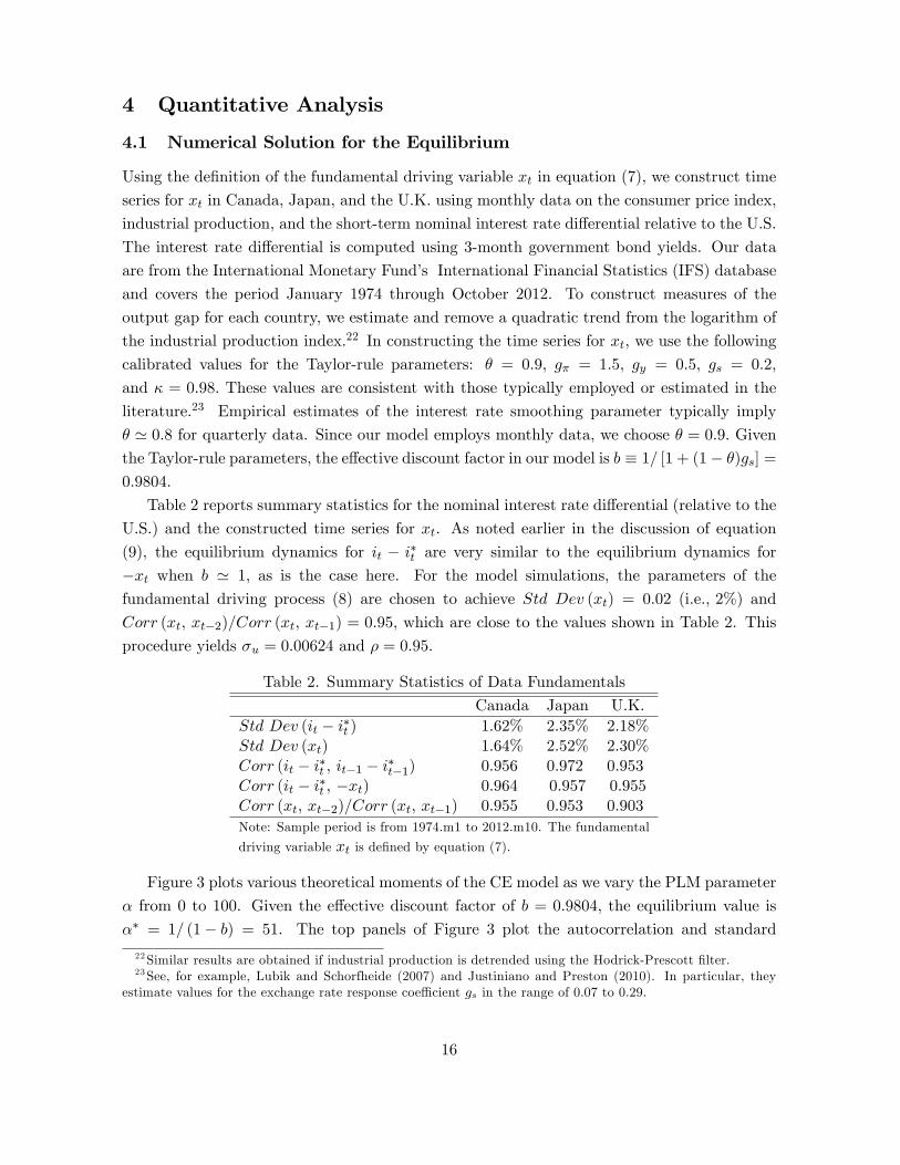
Table 2 reports summary statistics for the nominal interest rate di¤erential (relative to the

U.S.) and the constructed time series for xt. As noted earlier in the discussion of equation

(9), the equilibrium dynamics for it � i�t are very similar to the equilibrium dynamics for

�xt when b ' 1; as is the case here. For the model simulations, the parameters of the

fundamental driving process (8) are chosen to achieve Std Dev (xt) = 0:02 (i.e., 2%) and

Corr (xt; xt�2)=Corr (xt; xt�1) = 0:95; which are close to the values shown in Table 2. This

procedure yields �u = 0:00624 and � = 0:95:

Table 2. Summary Statistics of Data Fundamentals

Canada Japan U.K.Std Dev (it � i�t ) 1:62% 2:35% 2:18%Std Dev (xt) 1:64% 2:52% 2:30%Corr (it � i�t ; it�1 � i�t�1) 0:956 0:972 0:953Corr (it � i�t ; �xt) 0:964 0:957 0:955Corr (xt; xt�2)=Corr (xt; xt�1) 0:955 0:953 0:903

Note: Sample period is from 1974.m1 to 2012.m10. The fundamental

driving variable xt is de�ned by equation (7).

Figure 3 plots various theoretical moments of the CE model as we vary the PLM parameter

� from 0 to 100. Given the e¤ective discount factor of b = 0:9804; the equilibrium value is

�� = 1= (1� b) = 51. The top panels of Figure 3 plot the autocorrelation and standard

22Similar results are obtained if industrial production is detrended using the Hodrick-Prescott �lter.23See, for example, Lubik and Schorfheide (2007) and Justiniano and Preston (2010). In particular, they

estimate values for the exchange rate response coe¢ cient gs in the range of 0.07 to 0.29.

16

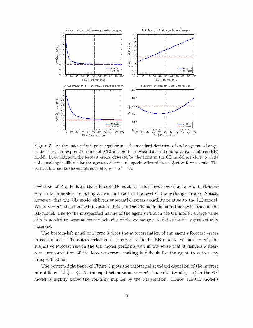
Figure 3: At the unique �xed point equilibrium, the standard deviation of exchange rate changesin the consistent expectations model (CE) is more than twice that in the rational expectations (RE)model. In equilibrium, the forecast errors observed by the agent in the CE model are close to whitenoise, making it di¢ cult for the agent to detect a misspeci�cation of the subjective forecast rule. Thevertical line marks the equilibrium value � = �� = 51:

deviation of �st in both the CE and RE models. The autocorrelation of �st is close to

zero in both models, re�ecting a near-unit root in the level of the exchange rate st: Notice,

however, that the CE model delivers substantial excess volatility relative to the RE model.

When � = ��; the standard deviation of �st in the CE model is more than twice that in the

RE model. Due to the misspeci�ed nature of the agent�s PLM in the CE model, a large value

of � is needed to account for the behavior of the exchange rate data that the agent actually

observes.

The bottom-left panel of Figure 3 plots the autocorrelation of the agent�s forecast errors

in each model. The autocorrelation is exactly zero in the RE model. When � = ��; the

subjective forecast rule in the CE model performs well in the sense that it delivers a near-

zero autocorrelation of the forecast errors, making it di¢ cult for the agent to detect any

misspeci�cation.

The bottom-right panel of Figure 3 plots the theoretical standard deviation of the interest

rate di¤erential it � i�t . At the equilibrium value � = ��; the volatility of it � i�t in the CEmodel is slightly below the volatility implied by the RE solution. Hence, the CE model�s

17

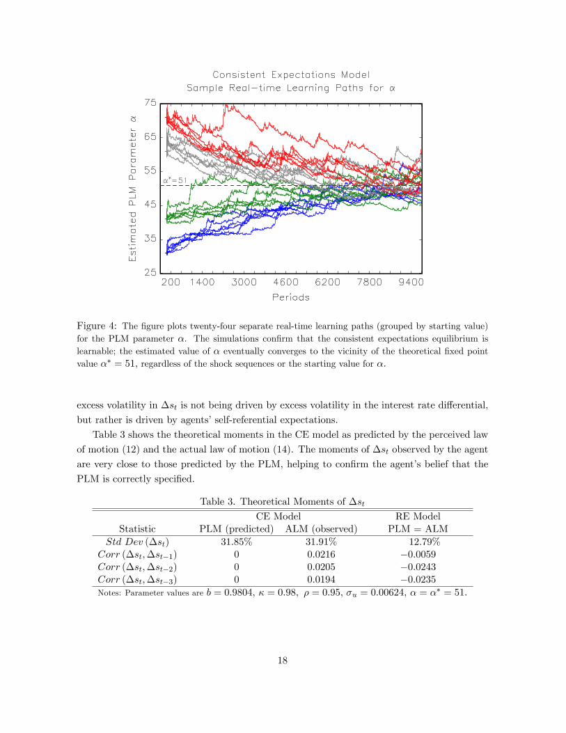
Figure 4: The �gure plots twenty-four separate real-time learning paths (grouped by starting value)for the PLM parameter �. The simulations con�rm that the consistent expectations equilibrium islearnable; the estimated value of � eventually converges to the vicinity of the theoretical �xed pointvalue �� = 51; regardless of the shock sequences or the starting value for �:

excess volatility in �st is not being driven by excess volatility in the interest rate di¤erential,

but rather is driven by agents�self-referential expectations.

Table 3 shows the theoretical moments in the CE model as predicted by the perceived law

of motion (12) and the actual law of motion (14). The moments of �st observed by the agent

are very close to those predicted by the PLM, helping to con�rm the agent�s belief that the

PLM is correctly speci�ed.

Table 3. Theoretical Moments of �stCE Model RE Model

Statistic PLM (predicted) ALM (observed) PLM = ALMStd Dev (�st) 31:85% 31:91% 12:79%

Corr (�st;�st�1) 0 0:0216 �0:0059Corr (�st;�st�2) 0 0:0205 �0:0243Corr (�st;�st�3) 0 0:0194 �0:0235Notes: Parameter values are b = 0:9804; � = 0:98; � = 0:95; �u = 0:00624; � = �

� = 51:

18

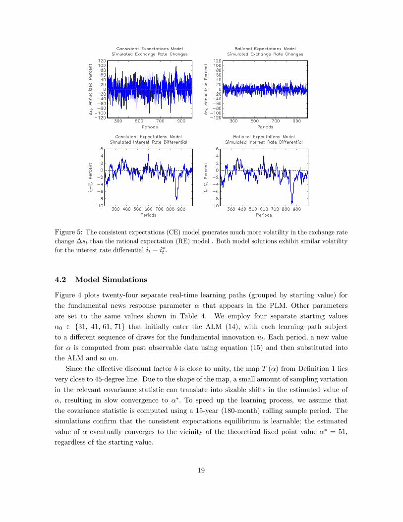
Figure 5: The consistent expectations (CE) model generates much more volatility in the exchange ratechange �st than the rational expectation (RE) model . Both model solutions exhibit similar volatilityfor the interest rate di¤erential it � i�t .

4.2 Model Simulations

Figure 4 plots twenty-four separate real-time learning paths (grouped by starting value) for

the fundamental news response parameter � that appears in the PLM. Other parameters

are set to the same values shown in Table 4. We employ four separate starting values

�0 2 f31; 41, 61, 71g that initially enter the ALM (14), with each learning path subject

to a di¤erent sequence of draws for the fundamental innovation ut: Each period, a new value

for � is computed from past observable data using equation (15) and then substituted into

the ALM and so on.

Since the e¤ective discount factor b is close to unity, the map T (�) from De�nition 1 lies

very close to 45-degree line. Due to the shape of the map, a small amount of sampling variation

in the relevant covariance statistic can translate into sizable shifts in the estimated value of

�, resulting in slow convergence to ��: To speed up the learning process, we assume that

the covariance statistic is computed using a 15-year (180-month) rolling sample period. The

simulations con�rm that the consistent expectations equilibrium is learnable; the estimated

value of � eventually converges to the vicinity of the theoretical �xed point value �� = 51;

regardless of the starting value.

19

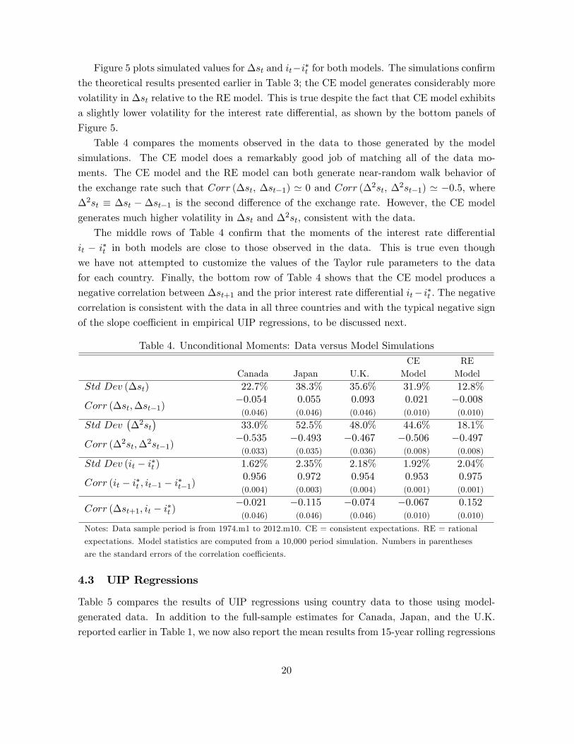
Figure 5 plots simulated values for�st and it�i�t for both models. The simulations con�rmthe theoretical results presented earlier in Table 3; the CE model generates considerably more

volatility in �st relative to the RE model. This is true despite the fact that CE model exhibits

a slightly lower volatility for the interest rate di¤erential, as shown by the bottom panels of

Figure 5.

Table 4 compares the moments observed in the data to those generated by the model

simulations. The CE model does a remarkably good job of matching all of the data mo-

ments. The CE model and the RE model can both generate near-random walk behavior of

the exchange rate such that Corr (�st; �st�1) ' 0 and Corr (�2st; �2st�1) ' �0:5; where�2st � �st � �st�1 is the second di¤erence of the exchange rate. However, the CE modelgenerates much higher volatility in �st and �2st; consistent with the data.

The middle rows of Table 4 con�rm that the moments of the interest rate di¤erential

it � i�t in both models are close to those observed in the data. This is true even thoughwe have not attempted to customize the values of the Taylor rule parameters to the data

for each country. Finally, the bottom row of Table 4 shows that the CE model produces a

negative correlation between �st+1 and the prior interest rate di¤erential it� i�t : The negativecorrelation is consistent with the data in all three countries and with the typical negative sign

of the slope coe¢ cient in empirical UIP regressions, to be discussed next.

Table 4. Unconditional Moments: Data versus Model Simulations

Canada Japan U.K.CEModel

REModel

Std Dev (�st) 22:7% 38:3% 35:6% 31:9% 12:8%

Corr (�st;�st�1)�0:054(0.046)

0:055(0.046)

0:093(0.046)

0:021(0.010)

�0:008(0.010)

Std Dev��2st

�33:0% 52:5% 48:0% 44:6% 18:1%

Corr (�2st;�2st�1)

�0:535(0.033)

�0:493(0.035)

�0:467(0.036)

�0:506(0.008)

�0:497(0.008)

Std Dev (it � i�t ) 1:62% 2:35% 2:18% 1:92% 2:04%

Corr (it � i�t ; it�1 � i�t�1)0:956(0.004)

0:972(0.003)

0:954(0.004)

0:953(0.001)

0:975(0.001)

Corr (�st+1; it � i�t )�0:021(0.046)

�0:115(0.046)

�0:074(0.046)

�0:067(0.010)

0:152(0.010)

Notes: Data sample period is from 1974.m1 to 2012.m10. CE = consistent expectations. RE = rational

expectations. Model statistics are computed from a 10,000 period simulation. Numbers in parentheses

are the standard errors of the correlation coe¢ cients.

4.3 UIP Regressions

Table 5 compares the results of UIP regressions using country data to those using model-

generated data. In addition to the full-sample estimates for Canada, Japan, and the U.K.

reported earlier in Table 1, we now also report the mean results from 15-year rolling regressions

20

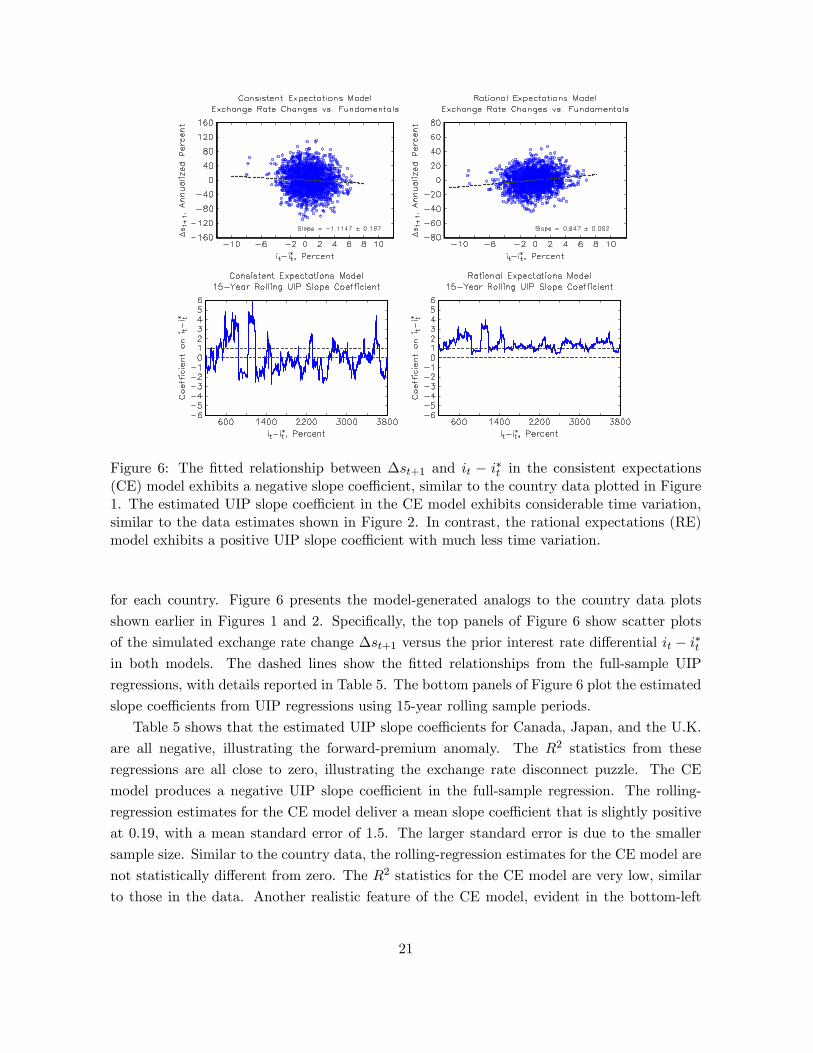
Figure 6: The �tted relationship between �st+1 and it � i�t in the consistent expectations(CE) model exhibits a negative slope coe¢ cient, similar to the country data plotted in Figure1. The estimated UIP slope coe¢ cient in the CE model exhibits considerable time variation,similar to the data estimates shown in Figure 2. In contrast, the rational expectations (RE)model exhibits a positive UIP slope coe¢ cient with much less time variation.

for each country. Figure 6 presents the model-generated analogs to the country data plots

shown earlier in Figures 1 and 2. Speci�cally, the top panels of Figure 6 show scatter plots

of the simulated exchange rate change �st+1 versus the prior interest rate di¤erential it � i�tin both models. The dashed lines show the �tted relationships from the full-sample UIP

regressions, with details reported in Table 5. The bottom panels of Figure 6 plot the estimated

slope coe¢ cients from UIP regressions using 15-year rolling sample periods.

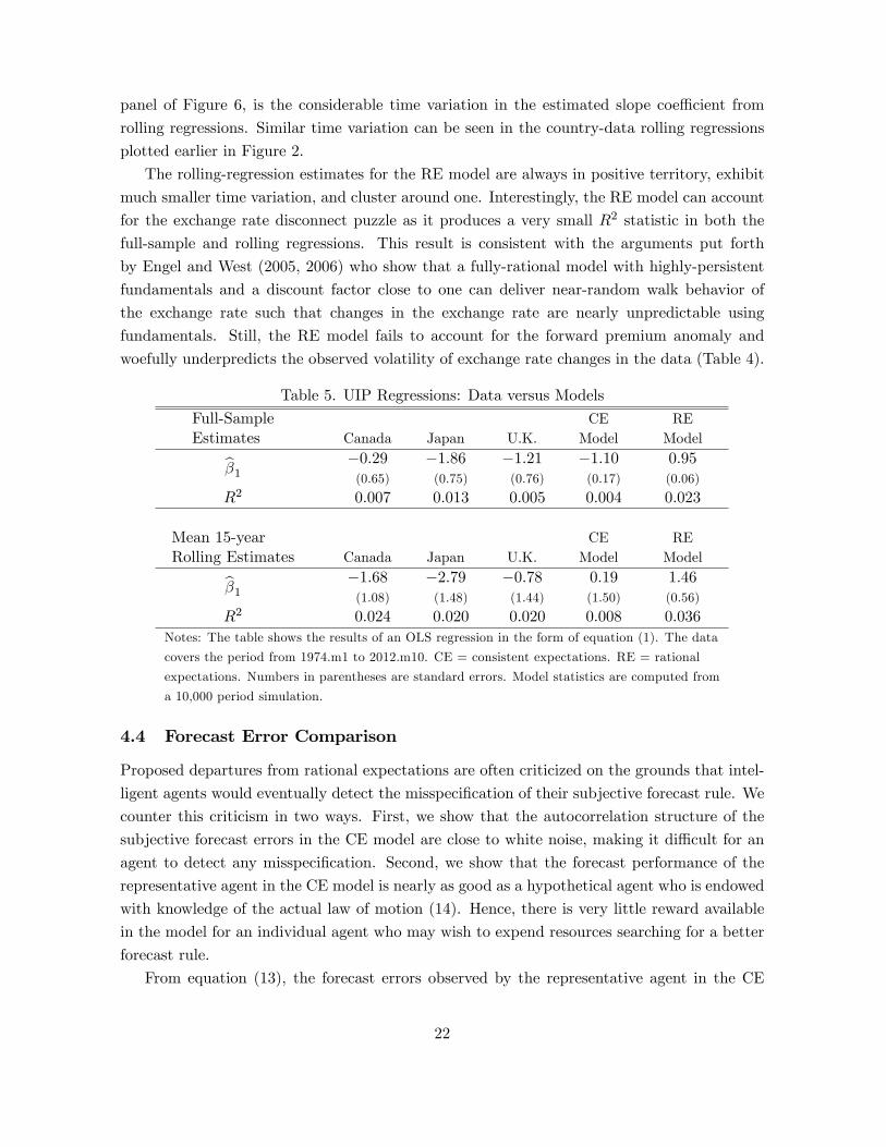
Table 5 shows that the estimated UIP slope coe¢ cients for Canada, Japan, and the U.K.

are all negative, illustrating the forward-premium anomaly. The R2 statistics from these

regressions are all close to zero, illustrating the exchange rate disconnect puzzle. The CE

model produces a negative UIP slope coe¢ cient in the full-sample regression. The rolling-

regression estimates for the CE model deliver a mean slope coe¢ cient that is slightly positive

at 0:19; with a mean standard error of 1.5. The larger standard error is due to the smaller

sample size. Similar to the country data, the rolling-regression estimates for the CE model are

not statistically di¤erent from zero. The R2 statistics for the CE model are very low, similar

to those in the data. Another realistic feature of the CE model, evident in the bottom-left

21

panel of Figure 6, is the considerable time variation in the estimated slope coe¢ cient from

rolling regressions. Similar time variation can be seen in the country-data rolling regressions

plotted earlier in Figure 2.

The rolling-regression estimates for the RE model are always in positive territory, exhibit

much smaller time variation, and cluster around one. Interestingly, the RE model can account

for the exchange rate disconnect puzzle as it produces a very small R2 statistic in both the

full-sample and rolling regressions. This result is consistent with the arguments put forth

by Engel and West (2005, 2006) who show that a fully-rational model with highly-persistent

fundamentals and a discount factor close to one can deliver near-random walk behavior of

the exchange rate such that changes in the exchange rate are nearly unpredictable using

fundamentals. Still, the RE model fails to account for the forward premium anomaly and

woefully underpredicts the observed volatility of exchange rate changes in the data (Table 4).

Table 5. UIP Regressions: Data versus Models

Full-SampleEstimates Canada Japan U.K.

CEModel

REModelb�1 �0:29

(0.65)

�1:86(0.75)

�1:21(0.76)

�1:10(0.17)

0:95(0.06)

R2 0:007 0:013 0:005 0:004 0:023

Mean 15-yearRolling Estimates Canada Japan U.K.

CEModel

REModelb�1 �1:68

(1.08)

�2:79(1.48)

�0:78(1.44)

0:19(1.50)

1:46(0.56)

R2 0:024 0:020 0:020 0:008 0:036

Notes: The table shows the results of an OLS regression in the form of equation (1). The data

covers the period from 1974.m1 to 2012.m10. CE = consistent expectations. RE = rational

expectations. Numbers in parentheses are standard errors. Model statistics are computed from

a 10,000 period simulation.

4.4 Forecast Error Comparison

Proposed departures from rational expectations are often criticized on the grounds that intel-

ligent agents would eventually detect the misspeci�cation of their subjective forecast rule. We

counter this criticism in two ways. First, we show that the autocorrelation structure of the

subjective forecast errors in the CE model are close to white noise, making it di¢ cult for an

agent to detect any misspeci�cation. Second, we show that the forecast performance of the

representative agent in the CE model is nearly as good as a hypothetical agent who is endowed

with knowledge of the actual law of motion (14). Hence, there is very little reward available

in the model for an individual agent who may wish to expend resources searching for a better

forecast rule.

From equation (13), the forecast errors observed by the representative agent in the CE

22

model are given by

errPLMt = st+1 � bE t st+1;= st+1 � st�1 � �ut; (21)

where we use the superscript �PLM�to indicate that bE t st+1 is based on the perceived law ofmotion (12). But of course, the evolution of st+1 is governed by the ALM (14).

Now consider an atomistic agent who understands that the evolution of st+1 is governed

by the ALM. This hypothetical agent cannot in�uence the evolution of st+1 but is tasked only

with making forecasts. The forecast error observed by the hypothetical agent is given by

errALMt+1 = st+1 � [1� (1� �)(1� b)] st � � xt; (22)

where we use the superscript �ALM� to indicate that the forecast is based on the actual

law of motion. Notice that, unlike the representative agent in the CE model, we allow the

hypothetical agent�s forecast to make use of the contemporaneous realization of the exchange

rate st:

Within the RE model, the forecast errors observed by the fully-rational agent are given by

errREt+1 = st+1 � (asst + ax�xt)

= axut+1: (23)

Given the sequences of forecast errors, it is straightforward to compute the associated auto-

correlations and the root mean squared forecast error, as given by RMSFE �qE[(errt+1)

2].

In each of the above cases, the forecasts are unbiased such that E (errt+1) = 0:

Table 6 compares the moments of the various forecast errors computed from model simu-

lations. For the PLM-based forecast, the autocorrelations of the forecast errors are near zero

at all lags, giving the agent in the CE model no signi�cant indication of a misspeci�cation.

The ALM-based forecast of the hypothetical agent delivers a slightly lower RMSFE of 31.8%

versus 32.1% for the PLM-based forecast. Hence, there is little room for an individual agent

in the CE model to improve forecasting performance by employing more sophisticated (and

presumably more costly) econometric methods to discover the true underlying law of motion

for the exchange rate.

The last column of Table 6 shows that the RE model exhibits the most accurate forecasts

(lowest RMSFE), as expected. However, it is important to realize that an individual agent

inhabiting the CE model could never achieve this level of forecast performance unless all of the

other agents decided to switch to the fully-rational forecast rule. This is because the actual

law of motion for the exchange rate in the CE model is permanently shifted by the forecasting

behavior of the CE agents.

23

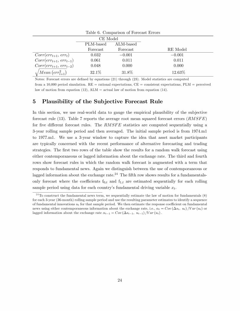
Table 6. Comparison of Forecast Errors

CE ModelPLM-basedForecast

ALM-basedForecast RE Model

Corr(errt+1; errt) 0:032 �0:001 �0:001Corr(errt+1; errt�1) 0:061 0:011 0:011Corr(errt+1; errt�2) 0:048 0:000 0:000qMean

�err2t+1

�32:1% 31:8% 12:63%

Notes: Forecast errors are de�ned by equations (21) through (23). Model statistics are computed

from a 10,000 period simulation. RE = rational expectations, CE = consistent expectations, PLM = perceived

law of motion from equation (12), ALM = actual law of motion from equation (14).

5 Plausibility of the Subjective Forecast Rule

In this section, we use real-world data to gauge the empirical plausibility of the subjective

forecast rule (13). Table 7 reports the average root mean squared forecast errors (RMSFE)

for �ve di¤erent forecast rules. The RMSFE statistics are computed sequentially using a

3-year rolling sample period and then averaged. The initial sample period is from 1974.m1

to 1977.m1. We use a 3-year window to capture the idea that asset market participants

are typically concerned with the recent performance of alternative forecasting and trading

strategies. The �rst two rows of the table show the results for a random walk forecast using

either contemporaneous or lagged information about the exchange rate. The third and fourth

rows show forecast rules in which the random walk forecast is augmented with a term that

responds to fundamental news. Again we distinguish between the use of contemporaneous or

lagged information about the exchange rate.24 The �fth row shows results for a fundamentals-

only forecast where the coe¢ cients f0;t and f1;t are estimated sequentially for each rolling

sample period using data for each country�s fundamental driving variable xt:

24To construct the fundamental news term, we sequentially estimate the law of motion for fundamentals (8)for each 3-year (36-month) rolling sample period and use the resulting parameter estimates to identify a sequenceof fundamental innovations ut for that sample period. We then estimate the response coe¢ cient on fundamentalnews using either contemporaneous information about the exchange rate, i.e., �t = Cov (�st; ut) =V ar (ut) orlagged information about the exchange rate �t�1 = Cov (�st�1; ut�1) =V ar (ut) :

24

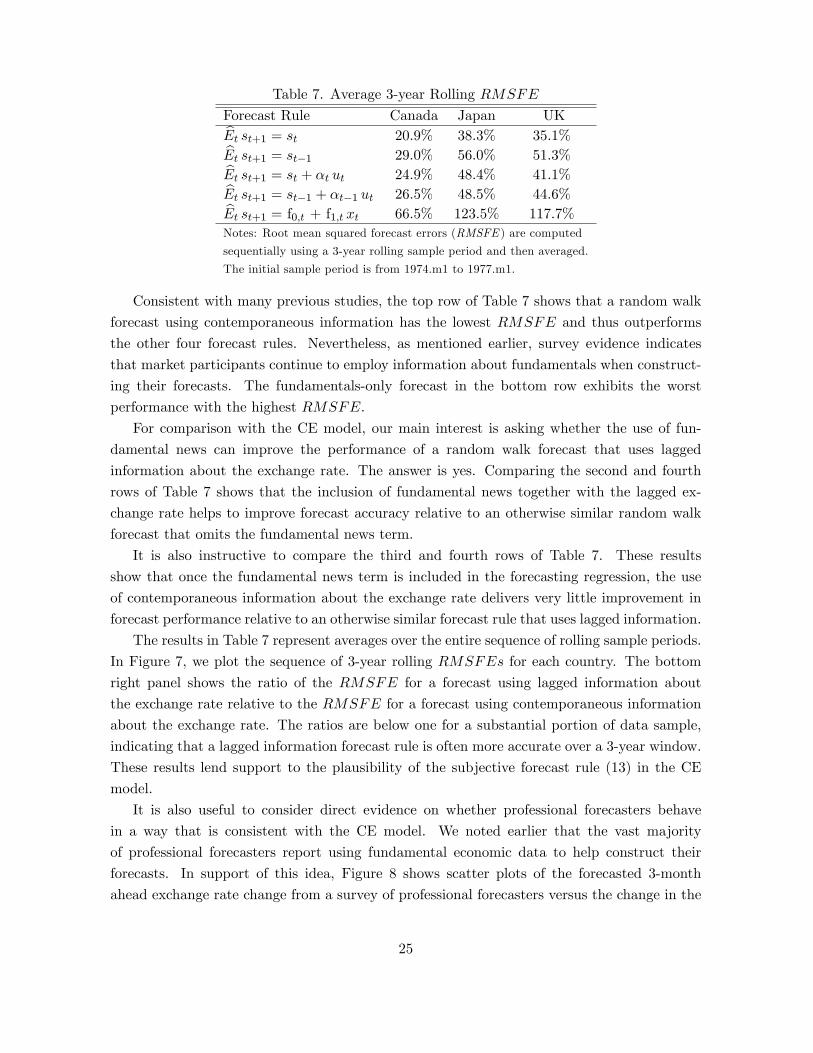
Table 7. Average 3-year Rolling RMSFE

Forecast Rule Canada Japan UKbEt st+1 = st 20:9% 38:3% 35:1%bEt st+1 = st�1 29:0% 56:0% 51:3%bEt st+1 = st + �t ut 24:9% 48:4% 41:1%bEt st+1 = st�1 + �t�1 ut 26:5% 48:5% 44:6%bEt st+1 = f0;t + f1;t xt 66:5% 123:5% 117:7%

Notes: Root mean squared forecast errors (RMSFE ) are computed

sequentially using a 3-year rolling sample period and then averaged.

The initial sample period is from 1974.m1 to 1977.m1.

Consistent with many previous studies, the top row of Table 7 shows that a random walk

forecast using contemporaneous information has the lowest RMSFE and thus outperforms

the other four forecast rules. Nevertheless, as mentioned earlier, survey evidence indicates

that market participants continue to employ information about fundamentals when construct-

ing their forecasts. The fundamentals-only forecast in the bottom row exhibits the worst

performance with the highest RMSFE.

For comparison with the CE model, our main interest is asking whether the use of fun-

damental news can improve the performance of a random walk forecast that uses lagged

information about the exchange rate. The answer is yes. Comparing the second and fourth

rows of Table 7 shows that the inclusion of fundamental news together with the lagged ex-

change rate helps to improve forecast accuracy relative to an otherwise similar random walk

forecast that omits the fundamental news term.

It is also instructive to compare the third and fourth rows of Table 7. These results

show that once the fundamental news term is included in the forecasting regression, the use

of contemporaneous information about the exchange rate delivers very little improvement in

forecast performance relative to an otherwise similar forecast rule that uses lagged information.

The results in Table 7 represent averages over the entire sequence of rolling sample periods.

In Figure 7, we plot the sequence of 3-year rolling RMSFEs for each country. The bottom

right panel shows the ratio of the RMSFE for a forecast using lagged information about

the exchange rate relative to the RMSFE for a forecast using contemporaneous information

about the exchange rate. The ratios are below one for a substantial portion of data sample,

indicating that a lagged information forecast rule is often more accurate over a 3-year window.

These results lend support to the plausibility of the subjective forecast rule (13) in the CE

model.

It is also useful to consider direct evidence on whether professional forecasters behave

in a way that is consistent with the CE model. We noted earlier that the vast majority

of professional forecasters report using fundamental economic data to help construct their

forecasts. In support of this idea, Figure 8 shows scatter plots of the forecasted 3-month

ahead exchange rate change from a survey of professional forecasters versus the change in the

25

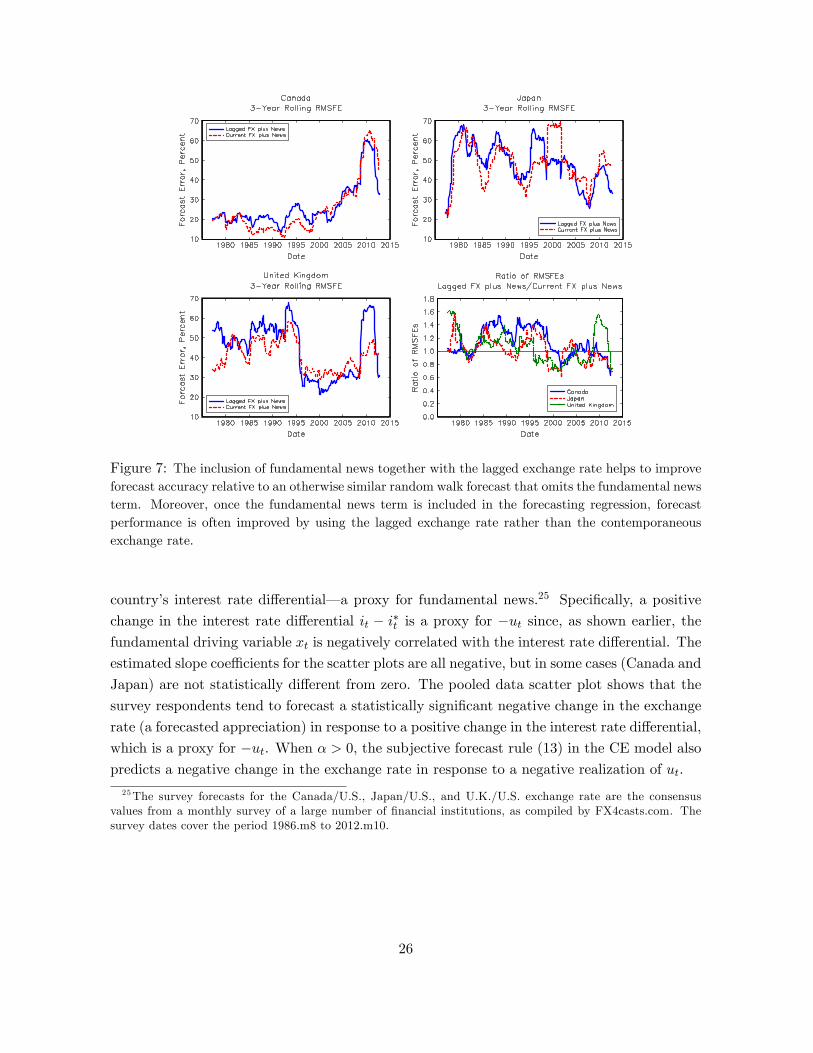
Figure 7: The inclusion of fundamental news together with the lagged exchange rate helps to improveforecast accuracy relative to an otherwise similar random walk forecast that omits the fundamental newsterm. Moreover, once the fundamental news term is included in the forecasting regression, forecastperformance is often improved by using the lagged exchange rate rather than the contemporaneousexchange rate.

country�s interest rate di¤erential� a proxy for fundamental news.25 Speci�cally, a positive

change in the interest rate di¤erential it � i�t is a proxy for �ut since, as shown earlier, thefundamental driving variable xt is negatively correlated with the interest rate di¤erential. The

estimated slope coe¢ cients for the scatter plots are all negative, but in some cases (Canada and

Japan) are not statistically di¤erent from zero. The pooled data scatter plot shows that the

survey respondents tend to forecast a statistically signi�cant negative change in the exchange

rate (a forecasted appreciation) in response to a positive change in the interest rate di¤erential,

which is a proxy for �ut. When � > 0, the subjective forecast rule (13) in the CE model alsopredicts a negative change in the exchange rate in response to a negative realization of ut:

25The survey forecasts for the Canada/U.S., Japan/U.S., and U.K./U.S. exchange rate are the consensusvalues from a monthly survey of a large number of �nancial institutions, as compiled by FX4casts.com. Thesurvey dates cover the period 1986.m8 to 2012.m10.

26

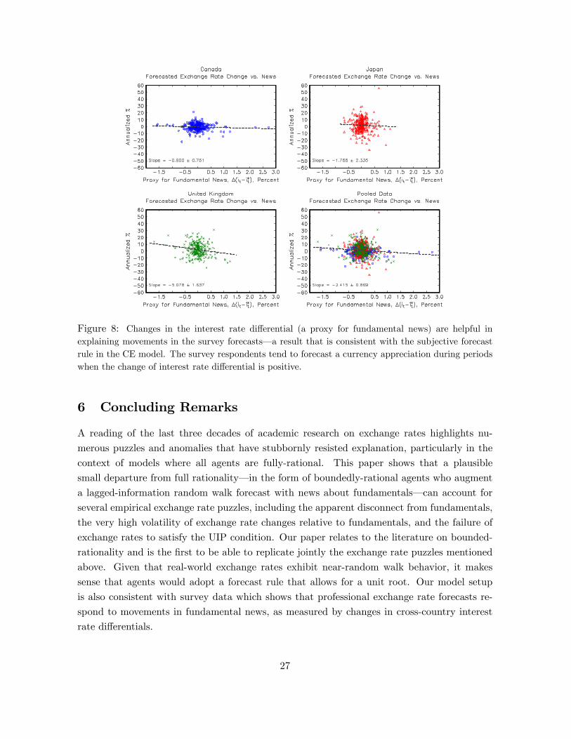
Figure 8: Changes in the interest rate di¤erential (a proxy for fundamental news) are helpful inexplaining movements in the survey forecasts� a result that is consistent with the subjective forecastrule in the CE model. The survey respondents tend to forecast a currency appreciation during periodswhen the change of interest rate di¤erential is positive.

6 Concluding Remarks

A reading of the last three decades of academic research on exchange rates highlights nu-

merous puzzles and anomalies that have stubbornly resisted explanation, particularly in the

context of models where all agents are fully-rational. This paper shows that a plausible

small departure from full rationality� in the form of boundedly-rational agents who augment

a lagged-information random walk forecast with news about fundamentals� can account for

several empirical exchange rate puzzles, including the apparent disconnect from fundamentals,

the very high volatility of exchange rate changes relative to fundamentals, and the failure of

exchange rates to satisfy the UIP condition. Our paper relates to the literature on bounded-

rationality and is the �rst to be able to replicate jointly the exchange rate puzzles mentioned

above. Given that real-world exchange rates exhibit near-random walk behavior, it makes

sense that agents would adopt a forecast rule that allows for a unit root. Our model setup

is also consistent with survey data which shows that professional exchange rate forecasts re-

spond to movements in fundamental news, as measured by changes in cross-country interest

rate di¤erentials.

27

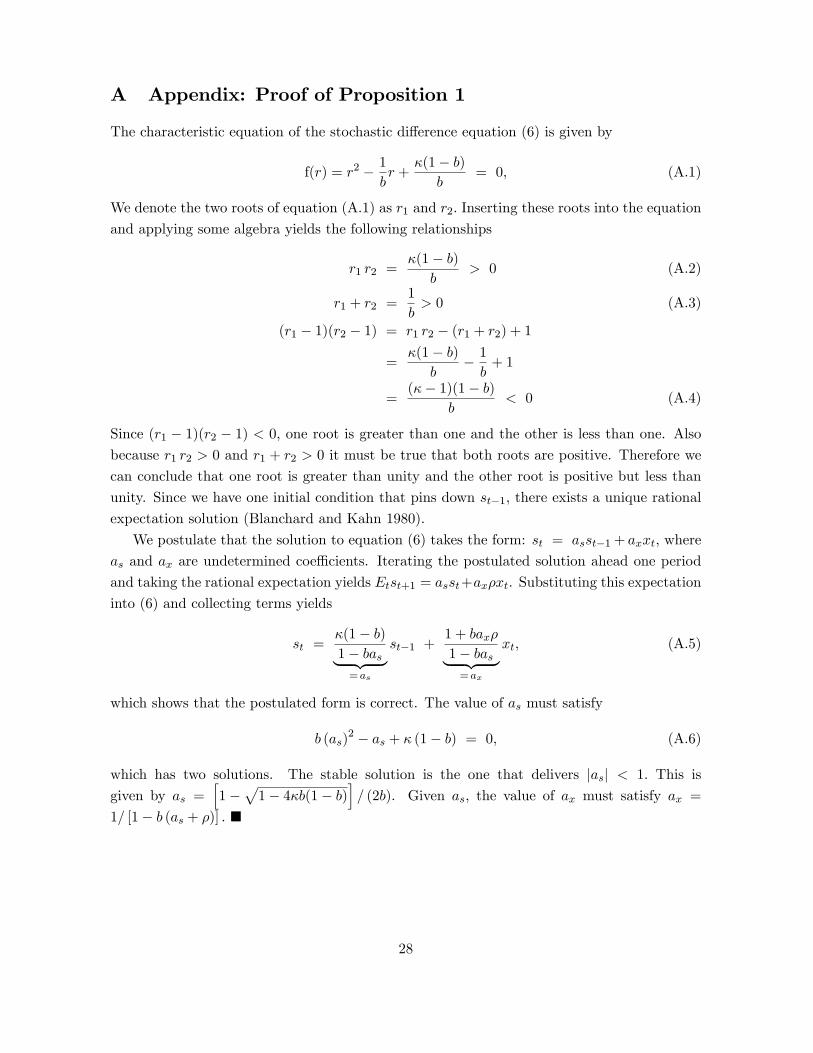
A Appendix: Proof of Proposition 1

The characteristic equation of the stochastic di¤erence equation (6) is given by

f(r) = r2 � 1br +

�(1� b)b

= 0; (A.1)

We denote the two roots of equation (A.1) as r1 and r2: Inserting these roots into the equation

and applying some algebra yields the following relationships

r1 r2 =�(1� b)

b> 0 (A.2)

r1 + r2 =1

b> 0 (A.3)

(r1 � 1)(r2 � 1) = r1 r2 � (r1 + r2) + 1

=�(1� b)

b� 1b+ 1

=(�� 1)(1� b)

b< 0 (A.4)

Since (r1 � 1)(r2 � 1) < 0; one root is greater than one and the other is less than one. Alsobecause r1 r2 > 0 and r1 + r2 > 0 it must be true that both roots are positive. Therefore we

can conclude that one root is greater than unity and the other root is positive but less than

unity. Since we have one initial condition that pins down st�1; there exists a unique rational

expectation solution (Blanchard and Kahn 1980).

We postulate that the solution to equation (6) takes the form: st = asst�1+ axxt, where

as and ax are undetermined coe¢ cients. Iterating the postulated solution ahead one period

and taking the rational expectation yields Etst+1 = asst+ax�xt. Substituting this expectation

into (6) and collecting terms yields

st =�(1� b)1� bas| {z }= as

st�1 +1 + bax�

1� bas| {z }= ax

xt; (A.5)

which shows that the postulated form is correct. The value of as must satisfy

b (as)2 � as + � (1� b) = 0; (A.6)

which has two solutions. The stable solution is the one that delivers jasj < 1: This is

given by as =h1�

p1� 4�b(1� b)

i= (2b). Given as; the value of ax must satisfy ax =

1= [1� b (as + �)] : �

28

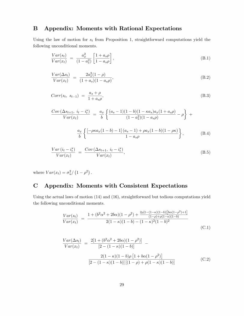
B Appendix: Moments with Rational Expectations

Using the law of motion for st from Proposition 1, straightforward computations yield the

following unconditional moments.

V ar(st)

V ar(xt)=

a2x(1� a2s)

�1 + as�

1� as�

�; (B.1)

V ar(�st)

V ar(xt)=

2a2x(1� �)(1 + as)(1� as�)

; (B.2)

Corr(st; st�1) =as + �

1 + as�; (B.3)

Cov (�st+1; it � i�t )V ar(xt)

=axb

�(as � 1)(1� b)(1� �as)ax(1 + as�)

(1� a2s)(1� as�)� �

�+

axb

�[���ax(1� b)� 1] (as � 1) + �ax(1� b)(1� ��)

1� as�

�; (B.4)

V ar (it � i�t )V ar(xt)

=Cov (�st+1; it � i�t )

V ar(xt); (B.5)

where V ar(xt) = �2u=�1� �2

�:

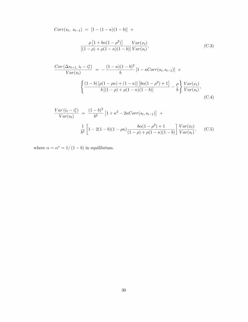
C Appendix: Moments with Consistent Expectations

Using the actual laws of motion (14) and (16), straightforward but tedious computations yield

the following unconditional moments.

V ar(st)

V ar(xt)=1 + (b2�2 + 2b�)(1� �2) + 2�[1�(1��)(1�b)][b�(1��2)+1]

(1��)+�(1��)(1�b)2(1� �)(1� b)� (1� �)2(1� b)2

(C.1)

V ar(�st)

V ar(xt)=2[1 + (b2�2 + 2b�)(1� �2)]

[2� (1� �)(1� b)] �

2(1� �)(1� b)��1 + b�(1� �2)

�[2� (1� �)(1� b)] [(1� �) + �(1� �)(1� b)] (C.2)

29

Corr(st; st�1) = [1� (1� �)(1� b)] +

��1 + b�(1� �2)

�[(1� �) + �(1� �)(1� b)]

V ar(xt)

V ar(st); (C.3)

Cov (�st+1; it � i�t )V ar(st)

= � (1� �)(1� b)2

b[1� �Corr(st; st�1)] +

((1� b) [�(1� ��) + (1� �)]

�b�(1� �2) + 1

�b [(1� �) + �(1� �)(1� b)] � �

b

)V ar(xt)

V ar(st);

(C.4)

V ar (it � i�t )V ar(st)

=(1� b)2b2

�1 + �2 � 2�Corr(st; st�1)

�+

1

b2

�1� 2(1� b)(1� ��) b�(1� �2) + 1

(1� �) + �(1� �)(1� b)

�V ar(xt)

V ar(st); (C.5)

where � = �� = 1= (1� b) in equilibrium.

30

ReferencesAdam, K., Evans, G.W., and Honkapohja, S., 2006. Are hyperin�ation paths learnable?,Journal of Economic Dynamics and Control 30, 2725-2748.Amromin, G. and Sharpe, S.A., 2014. From the horse�s mouth: economic conditions andinvestor expectations of risk and return, Management Science 60, 845-866.Andersen, T.G., Bollerslev, T., Diebold, F.X., and Vega, C., 2003. Micro e¤ects of macroannouncements: real-time price discovery in foreign exchange, American Economic Review93, 38-62.Bacchetta, P. and Van Wincoop, E., 2004. A scapegoat model of exchange rate �uctuations,American Economic Review, Papers and Proceedings 94, 114-118.Bacchetta, P. and Van Wincoop, E., 2007. Random walk expectations and the forward dis-count puzzle, American Economic Review, Papers and Proceedings 97, 346-350.Bacchetta, P. and Van Wincoop, E., 2013. On the unstable relationship between exchangerates and macroeconomic fundamentals, Journal of International Economics 91, 18-26.Baillie, R. and Chang, S., 2011. Carry trades, momentum Trading and the forward premiumanomaly, Journal of Financial Markets 14, 441-464.Baillie, R. and Cho, D., 2014. Time variation in the standard forward premium regression:some new models and tests, Journal of Empirical Finance 29, 52-63.Balke, N., Ma, J., and Wohar, M., 2013. The contribution of economic fundamentals tomovements in exchange rates, Journal of International Economics 90, 1-16.Bartolini, L. and Giorgianni, L., 2001. Excess volatility of exchange rates with unobservablefundamentals, Review of International Economics 9, 518-530.Blanchard, O.J. and Kahn, C.M., 1980. The solution of linear di¤erence models under rationalexpectations, Econometrica 48, 1305-1311.Burnside, C., 2011. The cross section of foreign currency risk premia and consumption growthrisk: comment, American Economic Review 101, 3456-3476.Burnside, C., Eichenbaum, M., and Rebelo, S., 2011. Carry trade and momentum in currencymarkets, Annual Review of Finance and Economics 3, 511-535.Burnside, C., Han, B., Hirshleifer, D., and Wang, T.Y., 2011. Investor overcon�dence and theforward premium puzzle, Review of Economic Studies 78, 523-558.Bansal, R., 1997. An exploration of the forward premium puzzle in currency markets, Reviewof Financial Studies 10, 369-403.Branch, W.A. and McGough, B., 2005. Consistent expectations and misspeci�cation in sto-chastic non-linear economies, Journal of Economic Dynamics and Control 29, 659-676.Campbell, J. and Cochrane, J., 1999. By force of habit: a consumption-based explanation ofaggregate stock market behavior, Journal of Political Economy 107, 205-251.Chakraborty, A. and Evans, G.W., 2008. Can perpetual learning explain the forward-premiumpuzzle?, Journal of Monetary Economics 55, 477-490.Cheung, Y-W., Chinn, M. D., and Pascual, A. G., 2005. Empirical exchange rate models of thenineties: are any �t to survive?, Journal of International Money and Finance 24, 1150-1175.Chinn, M., 2006. The (partial) rehabilitation of interest rate parity in the �oating rate era:longer horizons, alternative explanations, and emerging markets, Journal of InternationalMoney and Finance 25, 7-21.Cochrane, J.H., 1991. A critique of the application of unit root tests, Journal of EconomicDynamics and Control 15, 275-284.Coibion, O. and Gorodnichenko, Y., 2015. Information rigidity and the expectations formationprocess: a Simple framework and new facts, American Economic Review 105, 2644�2678

31

Dick, C.D. and Menkho¤, L., 2013. Exchange rate expectations of chartists and fundamental-ists, Journal of Economic Dynamics and Control 37, 1362�1383.Ding, L. and Ma, J., 2013. Portfolio reallocation and exchange rate dynamics, Journal ofBanking and Finance 37, 3100-3124.Engel, C., 1996. The forward discount anomaly and the risk premium: a survey of recentevidence, Journal of Empirical Finance 3, 123�191.Engel, C., 2014. Exchange rates and interest parity, in G. Gopinath, E. Helpman, and K.Rogo¤, (eds.), Handbook of International Economics Volume 4. Amsterdam: Elsevier, pp.453-516.Engel, C. and West, K., 2005. Exchange rates and fundamentals, Journal of Political Economy113, 485-517.Engel, C. and West, K., 2006. Taylor rules and the Deutschmark-Dollar real exchange rate,Journal of Money, Credit, and Banking 38, 1175-1194.Engel, C., Wang, J., and Wu, J., 2010. Long-horizon forecasts of asset prices when the discountfactor is close to unity, Working Paper.Evans, G.W. and Honkapohja, S., 2001. Learning and Expectations in Economics. Princeton:Princeton University Press.Evans, G.W. and Ramey, G., 2006. Adaptive expectations, underparameterization, and theLucas critique, Journal of Monetary Economics 53, 249-264.Fama, E., 1984. Forward and spot exchange rates, Journal of Monetary Economics 14, 319-338.Flood, R.P. and Rose, A.K., 2002. Uncovered interest rate parity in crisis, IMF Sta¤ Papers49, 252-266.Froot. K.A. and Thaler, R.H., 1990. Anomalies: foreign exchange, Journal of EconomicPerspectives 4(3), 179�192.Galí, J., Gertler, M., López-Salido, J.D., 2005. Robustness of the estimates of the Hybrid NewKeynesian Phillips Curve, Journal of Monetary Economics 52, 1107�1118.Gourinchas, P.-O. and Tornell, A., 2004. Exchange rate puzzles and distorted beliefs, Journalof International Economics 64, 303-333.Greenwood, R. and Shleifer, A., 2014. Expectations of returns and expected returns, Reviewof Financial Studies 27, 714-746.Huang, R., 1981. The monetary approach to exchange rate in an e¢ cient foreign exchangemarket: tests based on volatility, Journal of Finance 36, 31-41.Hommes, C., 2013. Behavioral Rationality and Heterogeneous Expectations in Complex Eco-nomic Systems. Cambridge: Cambridge University Press.Hommes, C. and Sorger, G., 1998. Consistent expectations equilibria, Macroeconomic Dy-namics 2, 287-321.Hommes, C. and Zhu, M., 2014. Behavioral learning equilibria, Journal of Economic Theory150, 778-814.Ilut, C., 2012. Ambiguity aversion: implications for the uncovered interest rate parity puzzle,American Economic Journal: Macroeconomics 4, 33-65.Justiniano, A. and Preston, B., 2010. Monetary policy and uncertainty in an empirical smallopen-economy model, Journal of Applied Econometrics 23, 93-128.Ko, H.-H. and Ogaki, M., 2015. Granger causality from exchange rates to fundamentals: whatdoes the bootstrap test show us? International Review of Economics & Finance 38, 198-206.Koijen, R.S.J., Schmeling, M, and Vrugt, E.B., 2015. Survey expectations of returns and assetpricing puzzles, Working Paper.

32

Mankiw. N.G., and Reis, R., 2002. Sticky information versus sticky prices: a proposal toreplace the New Keynesian Phillips Curve, Quarterly Journal of Economics 117, 1295-1328.Lansing, K.J., 2009. Time-varying U.S. in�ation dynamics and the New Keynesian PhillipsCurve, Review of Economic Dynamics 12, 304-326.Lansing, K.J., 2010. Rational and near-rational bubbles without drift, Economic Journal 120,1149-1174.Lubik, T.A. and Schorfheide, F., 2007. Do central banks respond to exchange rate movements?A structural investigation. Journal of Monetary Economics 54, 1069-1087.Lustig, H. and Verdelhan, A., 2007. The cross section of foreign currency risk premia andconsumption growth risk, American Economic Review 97, 89-117.Lustig, H., Roussanov, N., and Verdelhan, A., 2014. Countercyclical currency risk premia,Journal of Financial Economics.111, 527�553Mark, N., 2009. Changing monetary policy rules, learning, and real exchange rate dynamics,Journal of Money, Credit, and Banking 41, 1047-1070.Meese, R. A., and Rogo¤, K., 1983. Empirical exchange rate models of the seventies: do they�t out of sample? Journal of International Economics 14, 3-24.Nerlove, M., 1967. Distributed lags and unobserved components in economic time series, inW. Fellner, (ed.), Ten Economic Studies in the Tradition of Irving Fischer. New York: JohnWiley & Sons, pp. 127-169.Rossi, B., 2013. Exchange rate predictability, Journal of Economic Literature 51, 1063-1119.Sarno, L., 2005. Viewpoint: towards a solution to the puzzles in exchange rate economics:where do we stand? Canadian Journal of Economics 38, 673-708.Sögner, L. and Mitlöhner, H., 2002. Consistent expectations equilibria and learning in a stockmarket, Journal of Economic Dynamics and Control 24, 799-831.Ter Ellen, S., Verschoor, W.F.C., and Zwinkels, R.C.J., 2013. Dynamic expectation formationin the foreign exchange market, Journal of International Money and Finance 37, 75-97.Verdelhan, A., 2010. A habit-based explanation of the exchange rate risk premium, Journalof Finance 65, 123-145.Wadhwani, S.B., 1987. Are exchange rates �excessively� volatile? Journal of InternationalEconomics 22, 339-348.West, K., 1987. A standard monetary model and the variability of the Deutschemark-Dollarexchange rate, Journal of International Economics 23, 57-76.Yu, J., 2013. A sentiment-based explanation for the forward premium puzzle, Journal ofMonetary Economics 60, 474-491.

33