Experimentation Speed Across Products: Evidence from Peru in

the USA Market

Manuel Tong Koecklin∗

University of Sussex

June 25, 2017

Abstract

This paper develops a model to explain how quickly exporters sequentially export prod-ucts to a particular destination in a setting where product demands follow a joint bivariatedistribution. By exporting shipments of a first product A to market d and observing realiseddemand, the exporter gradually updates his perceived demand for product B. Expectedprofitability of product B, and thus the decision to export, is shown to be a function of thenumber of shipments of A, the correlation coefficient between the two demands, as well asthe mean export value of A. Sequential exporting is predicted to take place faster (afterfewer shipments of product A) if (i) trade costs of product B are lower, (ii) the mean value ofA exports is larger, and (iii) the higher is the correlation between product demand in marketd. This prediction is then tested by a survival analysis, using a rich dataset of Peruvian firmsthat exported to the United States between 2006 and 2013. The enactment of the USA-PeruFree Trade Agreement in 2009, which eliminated most tariffs on Peruvian products in USA,is associated with an acceleration of the introduction of new products into that market,expressed as either fewer shipments of previous products or a shorter time spell betweenthe first shipments of the old and the new product. Such acceleration tends to be largerfor products with higher pre-FTA tariffs that were not included in pre-FTA unilateral tradepreferences by USA. Additionally, trade liberalisation tends to facilitate the introduction ofnew products by pre− FTA firms after having sent smaller values of previous products.

Keywords: Export dynamics, experimentation, trade liberalisation, number of shipments,survival analysis, USA-Peru Free Trade Agreement

JEL Classification: F14, D21, F15, D22

1 Introduction

Recent literature on firm export dynamics has found that firms surviving in the export activitytend to experiment sequentially in the foreign market; but what is their experimentation speedin that activity? And what factors determine that speed?

Albornoz et al. (2012) is one of the first studies on export sequential strategy, finding thatnew Argentinean exporters, despite having a higher probability of exiting the export business,

∗University of Sussex, Jubilee Building, Falmer, Brighton, United Kingdom. +44 7810315872.mt338@sussex.ac.uk

1

grow more at the intensive and extensive margin, conditional on survival, compared to moreestablished exporters. That is, surviving new exporters undertake a sequential exporting process.

Those described dynamics occur across destinations, leaving as a pending concern how dy-namics in export decisions by firms work within one destination, across products. Moreover,the way trade liberalisation may affect those decisions remains insufficiently addressed.

Works like Albornoz et al. (2012) obtain that, by realising the export profitability in onemarket, firms may sequentially decide to sell to further destinations. However, that decisionmay actually be delayed, both across markets and products within one destination. How longdo firms take to introduce a new product to a particular market? What factors determine theacceleration or delay of that decision? Does trade liberalisation play a role in this process?

Other studies on firm export dynamics focus on firms’ probability to survive and/or exit theexport activity. Roberts and Tybout (1997) and Eaton et al. (2008) describe the export entryand exit decision processes for Colombian firms. In the Peruvian context, Freund and Pierola(2010) theoretically explains the export entry determinants in terms of costs; while Malca andRubio (2012) addresses the role of tenure as a driver of firms’ export survival.

In that same line, other researches measure the duration of firms’ permanence in the exportactivity and its determinants, by applying conventional methods like the Kaplam-Meier survivalestimator or the Cox proportional hazard model. Indeed, Besedes and Prusa (2006b) usethese approaches to explore the role of product differentiation in the duration of USA importrelationships. Volpe Martincus and Carballo (2008), with the same techniques, analyse theeffect of product and geographical diversification, along with firm size, on the survival likelihoodof Peruvian firms in the export business.

Even in the literature on multi-product firms, the use of survival or duration models ispractically limited to examining the survival of products in a firm’s export portfolio. To myknowledge, no previous works on firm export dynamics have applied those methods under a morepositive focus. One in which the event of entering into the export activity, i.e. a success, isanalysed. One example is the decision to introduce a new product into a particular destination.

There is also a growing literature on experimentation in different areas, whereby the decisionto undertake one particular action may be delayed, by gradually updating agents’ beliefs on thepayoff from that action. The use of that approach to illustrate firms’ export strategies is quiterecent, either by the role of learning from neighbour firms, like Fernandes and Tang (2014),or firms’ previous experience in other markets, like Akhmetova and Mitaritonna (2012) andNguyen (2012). Hence, firms’ decision to introduce a new product to a market of interest byupdating their beliefs on the demand for that product, given their previous experiences withother goods in that destination, is a subject of potential research under that approach.

Given the described gaps, this paper contributes to the literature by developing a theoreticalmodel, empirically tested afterwards, explaining how quickly firms sequentially export productsto a particular destination, incorporating the role of trade liberalisation and the firms’ experiencewith other products in the market of interest. That is, what is the experimentation speed offirms across products in a market? In my approach, such speed is measured by the number ofshipments of product A to market d by firm i required before deciding to introduce productB to that market. Hence, the fewer shipments of A prior to introducing B, the quicker theexperimentation will be. The role of trade liberalisation in this scheme is accounted for as thetariff elimination by the market of interest on products from the country of origin.

I test the prediction from my theoretical model by a survival analysis, using a very richdataset of Peruvian firms that exported to the United States between 2006 and 2013. I exploit

2

the nature of my dataset, which is at the transaction level, by constructing observations, eachone representing the event in which a Peruvian firm introduces a one or many new productsto the USA market, henceforth called an experimentation round. The Peru-USA case is anappropriate one for this research, since the two countries signed a Free Trade Agreement in2009, and long discussions arose on the new opportunities and potential threats to the Peruvianmanufacturing industry. Yet, little is known on the effects of this trade liberalisation processon the performance of Peruvian firms in that market.

By this analysis, not only do I measure the experimentation speed of Peruvian firms acrossproducts in the USA market. I also investigate whether the tariff elimination by USA onPeruvian products under the USA-Peru FTA plays an accelerating role in firms’ decision tointroduce a new product to that destination. This role can be assessed by comparing (1)firms founded before and after the FTA enactment; (2) experimentation rounds occurred beforeand after such enactment; (3) the original tariffs levied on the products introduced; or (4)the treatment given by USA to the product before the FTA (whether the products enjoyeda unilateral trade preference). Additionally, I examine if a firm’s large prior experience withother products in USA, expressed as a high mean export shipments of old products, exerts anaccelerating effect on the decision to experiment with a new product.

My empirical approach embraces a Kaplan-Meier survival estimator, as well as a Cox pro-portional hazard model, where my time variable is the number of days before the firm’s exper-imentation round i in USA, counting from the day round i− 1 occurred, or firm’s foundation.I also run OLS and panel data regressions at the experimentation round level, where my de-pendent variable is the number of shipments of product A before the introduction of productB to USA by a firm. Overall, the results find that trade liberalisation is associated with anacceleration of the introduction of new products into that market. Such acceleration tends tobe larger for products with higher pre-FTA tariffs that were not included in pre-FTA unilateraltrade preferences by USA, such as the ATPDEA regime or the MFN zero tariff. Moreover, inthe case of firms founded before the FTA enactment, trade liberalisation tends to facilitate theintroduction of new products after having sent smaller values of previous products.

The remainder of the paper is organised as follows. Section 2 goes deeper into the relatedliterature. Section 3 presents the theoretical model. Section 4 describes the data and offers adescriptive analysis of Peruvian firms exporting to the USA market, focusing on their experi-mentation rounds. Section 5 presents the Kaplan-Meier survival analysis. Section 6 shows theresults from my econometric approach. Section 7 concludes.

2 Related Literature

Three large strands of the previous literature clearly nourish my research: (i) firm exportdynamics, (ii) multi-product firms and (iii) experimentation.

2.1 Firm Export Dynamics

Within the growing literature on firm export dynamics, I highlight the recent interest in thesequential exporting strategy undertaken by firms in the foreign market.

Albornoz et al. (2012), which inspires part of my theoretical approach, is one of the firstresearches on that issue, focusing on the Argentinean industry. In line with previous researches,these authors argue that many new exporters give up very shortly after entering, despite having

3

incurred substantial entry costs; while others raise sales and expand to new destinations. Theyassume that a firm’s export profitability is initially uncertain, only realised once it enters theexport market, paying a fixed entry cost. Such export profitability is perfectly correlated overtime and across destinations, and its discovery leads to a sequential exporting process, wherebyfirms use their initial export experience to infer information on their potential success in thisand other markets.

This compelling analysis is undertaken across markets, leaving unattended how these dy-namics operate within one destination, i.e. how firms develop their strategy across products.Furthermore, the trade liberalisation issue is yet to be accounted for in that analysis.

Like Albornoz et al. (2012) most literature reviewed on firm export dynamics cover the firmdecision to enter and exit the export activity, and its progress across destinations. Robertsand Tybout (1997), for instance, quantified the effect of prior exporting experience on Colom-bian manufacturing plants’ decision to enter into foreign markets, finding that after a two-yearabsence, re-entry costs are as similar as those of a new exporter, due to export experience de-preciation. Moreover, larger and older plants are all more likely to export. Eaton et al. (2008),also for the Colombian case, observe that, while many firms start and stop exporting, exportsales are dominated by a few very large and stable firms.

Some studies address the Peruvian case, such as Freund and Pierola (2010), which showsa considerable entry and exit flows of Peruvian exporters each year. However, contrary to Al-bornoz et al. (2012), they argue that smaller firms can discover their entry costs by a very cheaptrial, while firm size is positively associated with large export sales. In contrast, developing newproducts requires a much larger entry cost. Also focusing on the Peruvian industry (agricul-ture), Malca and Rubio (2012) analyse the relation between tenure in export markets andexport performance, finding that for one additional year a firm exports, there is a considerablerise in the probability of remaining as an exporter (survival).

The latter leads to refer to a growing tendency to the use of duration models to measurefirms’ probability to remain or exit from the export activity. Besedes and Prusa (2006a), forinstance, address the duration of US imports from up to 180 countries, finding a short medianduration of about 2 or 4 years. They also obtain a negative duration dependence; that is, if acountry can survive exporting for the first few years, its failure probability falls, maintainingits trade relation.

Other studies like Besedes and Prusa (2006b) use more conventional survival analysis meth-ods like the Kaplan-Meier estimator and the Cox proportional hazard models. These authorsfind that US import trade relationships involving differentiated products have over twice as longa median duration as other product types starting with considerably smaller initial purchases.The larger these initial purchases, the longer the duration, and the larger the differences acrossproduct types. For the Peruvian case, Volpe Martincus and Carballo (2008) use both methodsconsidering only new exporters, finding that both product and, especially, geographical diver-sification raise the chances of remaining an exporter. Larger firms, measured by number ofemployees, are more likely to survive in foreign markets. 1

Despite the valuable findings from these studies, there is a limited consideration of tradeliberalisation into the analysis of firm export dynamics. 2 Moreover, the cited papers on the

1Many other studies analyse export survival by employing the aforementioned approaches, such as Besedesand Blyde (2010) for Latin America and Carrere and Strauss-Kahn (2014) for non-OECD countries. Otherstudies explore alternative methods like discrete-time models ( Hess and Persson (2012)), or the Prentice andGloeckler (1978) model ( Brenton et al. (2010)).

2 Brenton et al. (2010), for instance, only introduces a dummy for countries signing a Regional Trade

4

Peruvian case have not addressed the recent enactment of the USA-Peru Free Trade agreementand other treaties. Hence, there is a huge potential to explore these issues and, from thecommented Besedes and Prusa (2006b) findings, we can also ask how the relationship betweenexport size and duration vary across products.

Additionally, all studies listed herein, utilising duration models, took the conventional pro-cess of considering the event of firms leaving the export market as the “failure” of interest.What about, instead, addressing a positive event of interest, for instance, how long it takes forfirms to decide to enter into the export activity?

2.2 Multi-Product Firms

Since my focus is firms’ export strategy across products in one destination, the event of interestI am interested in is the introduction of a new product into a foreign market. Therefore, it isnecessary to refer to the literature on multi-product firms. Within this strand, works likeEckel and Neary (2010), Eckel et al. (2009) and Mayer et al. (2011), on the role of “corecompetence” products in a context of trade liberalisation, clearly stand out, but most of themare limited to a single-year analysis at a firm level, rather than at a wider firm-product level.

Other studies follow the performance of multi-product firms in a longer period, such asJavorcik and Iacovone (2008), which presents stylised facts of firm-product dynamics in theMexican industry during an export boom. The authors find, among other facts, that newexporters tend to “start small” in value and number of products, and the introduction of newproducts is preceded by a surge in investment. Equally important, the intensive and extensivemargin across products are positively correlated.

A valuable theoretical contribution on firms’ dynamics across products is provided by Bernardet al. (2010), on the frequency, pervasiveness and determinants of product switching. The au-thors predict that the duration of a product in a firm’s product mix is longer the greater thesale volume and the longer the tenure of the product; that the exit probability of a firm-productcombination is decreasing in productivity and quality; and that the product adding and drop-ping rates are positively correlated. Motivated by that framework, Gorg et al. (2012) analysesthe determinants of products’ survival in Hungarian firms’ export mixes. Departing from theidea that product choices are endogenous, they find that both firm and product characteristicsmatter in export dynamics. In fact, firm productivity, as well as product scale and tenure, isassociated with higher export survival rates.

Another remarkable theoretical approach is found at Bernard et al. (2006), which incor-porates the role of trade liberalisation. Here, firm productivity is a combination of firm-level“ability” and firm-product-level “expertise”, both unknown until the firm pays a sunk cost of en-try. The authors conclude that higher “ability” raises a firm’s productivity across all products,inducing a positive correlation between firm’s intensive and extensive margins. Trade liberali-sation fosters productivity growth within and across firms and in aggregate, because firms dropmarginally productive products and the least productive firms exit. However, surviving firmsincrease their share of products sold abroad, as well as their exports per product. In that line,Arkolakis and Muendler (2010), makes an empirical test with cross sectional Brazilian data,obtaining results akin to the predictions described earlier.

These works, more focused on the firm-product level, offer a valuable contribution on thedeterminants of products’ survival in firms’ export mix. However, I propose to evaluate a

Agreement–, leaving room for further research.

5

different phenomenon. What determines firms’ decision to introduce a product or set of productsinto one particular destination, and how long does it take for this event to occur? In other words,I am interested in measuring firms’ experimentation speed in one market. And one departurepoint to consider comes from a literature survey by Bernard et al. (2011). They make referenceto studies finding that firms update their priors about profitability in export markets, basedupon their sales, deciding to exit or expand their penetration of export markets over time.

2.3 Experimentation

The point raised earlier leads me to refer to the literature on experimentation . This stranddates back to a first model by Wald (1945), illustrating sequential tests of statistical hypotheses.In this process, we may decide either to accept a null hypothesis, reject it, or continue theexperiment by making an additional observation. That process terminates when one of thefirst two decisions is made; but will continue if we opt for the third. Thus, a sequential test isundertaken, where the number of observations is a random variable, unlike other tests where thatnumber is predetermined. The author argues this test is more efficient as the expected numberof observations required is lower.3 Extensions to this approach can be found at Moscariniet al. (1998), aiming to find an optimal experimentation level, assuming the decision maker isimpatient, making variable-size experiments each period, at some increasing and strictly convexcost before making a final decision. That optimal level is increasing in the confidence about theproject outcome and for more impatient agents.

These basic ideas were further deployed in contexts like the decision to adopt new agriculturaltechnologies in Ghana ( Conley and Udry (2001)) and India ( Foster and Rosenzweig (1995))or the modelling of entrepreneurial learning ( Minniti and Bygrave (2001)). The first twofocus on belief updates depending on neighbours’ performance.4 Other studies, like Kellyand Kolstad (1999) on growth and pollution, emphasise that decision makers have a Bayesianlearning process. This theoretical approach addresses the relation between greenhouse gas levelsand global mean temperature changes. Policy makers learn depending on stochastic shocks tothe realised temperature, and the expected learning time is related to the variance of that shockand the emissions policy, implying a tradeoff between emissions control and learning speed.

Closer to my focus are Rauch and Watson (2003) and Watson (1999) on “starting small”in a trade partnership. The former, theoretically portraying the relation between a developedcountry buyer and a developing country supplier, states that matched firms “start small” toassess the supplier’s ability to successfully fulfil a large order. That propensity rises withthe cost of seeking a new supplier, and falls with the probability of fulfilling a large order aftertraining. The latter incorporates renegotiation into the analysis, making both agents decide withincomplete information whether to cooperate or betray each other. They find an equilibriumwhere partners “start small”, uniquely selected under a strong renegotiation condition.

More into the exports matter is Fernandes and Tang (2014) on how learning from neigh-bouring firms affects new exporters’ performance, updating their prior belief on a foreign marketdemand, based on the number of exporting neighbours, export heterogeneity and the firm’s ownbelief. A positive signal from neighbours increases the firm’s probability to enter a market andits initial sales, and that effect is stronger the more exporting neighbours and the less familiarto the market the firm is.

3 Wald (945a) provides more practical examples of this test.4 Bolton and Harris (1999) provides a theoretical approach in which N decision makers learn from each other’s

experimentations, deciding between a “safe” and a “risky” action.

6

Another approach is in terms of number of destinations explored. Akhmetova and Mi-taritonna (2012) propose an experimentation model whereby a firm can postpone full entryinto a market and learn more about its product’s demand by accessing a few consumers. Thefirm chooses an optimal experimentation intensity (number of consumers accessed) and an en-try/exit policy. That intensity will be larger if the firm is more productive, even if its beliefsare low. Empirically, these predictions are proven in a context of testing destinations beforefully entering into a region.

But the closest work to my interest, inspiring part of my theoretical model, is Nguyen(2012), explaining why firms wait to export and why many fail. Its key assumption is imperfectcorrelation of demand across destinations, so that firms can use previously realised demandsfrom other markets to forecast demands from untested destinations. This gives firms the chanceto delay exporting to a particular market, by gathering information from already explored mar-kets. Thus, firms opt for entering markets sequentially, entering and exiting destinations afterrealising their demands. A similar rationale I propose to apply to explaining firms’ experimen-tation strategy within one destination, by introducing new products sequentially. Thus, I cantheoretically measure how long it takes for a firm, after selling one new product to the market ofinterest, to sell another one, expressed as the number of shipments of the previous new productprior to the first shipment of the next one. In other words, I aim to measure firms’ experimen-tation speed in a market and its determinants, including the role of trade liberalisation. Notethat Nguyen (2012) does not consider the influence of other firms. I follow this feature in myapproach, as I am more interested in the transition from the first to the second and subsequentnew products, rather than the decision to export the first product.

3 Theoretical Model

The basics of my theoretical model are inspired from a previous study by Albornoz et al. (2012)on sequential exporting across markets.

A producer from country o evaluates to export or not to country d, with a product portfolioconsisting of products A and B. If the firm decides to enter d, it will have to pay a sunk entrycost Fd per product, assumed to the identical across products, meant to reflect distributionchannels, marketing strategy and exporting procedures, which might be specific to each kindof product. I assume other common entry costs across products within a market, such asinformation on institutional and policy characteristics of the foreign country, to be minimaland/or easily accessible to firms.

When exporting products A and B to country d, firms must pay a product-specific unit tradecost (tariff levied by d) τA and τB, such that τA ≤ τB.5 Variable costs per product comprisea unit export cost, cAx and cBx , and a firm-specific unit production cost, cAp and cBp , such that

cAp > cBp , which means that a firm is more efficient producing B than A. This implies that goodB is the firm’s core competence product; the good in which the firm is more productive. Whileproduction costs are known to the firm, unit export costs are unknown.

The demand side, on the other hand, is represented by the following function:

qj(pj) = dj − pj (1)

where qj denotes the quantity of product A or B exported; pj is the price of that product; and

5I make the assumption that home firm pays the tariff, since I do not have information on importers.

7

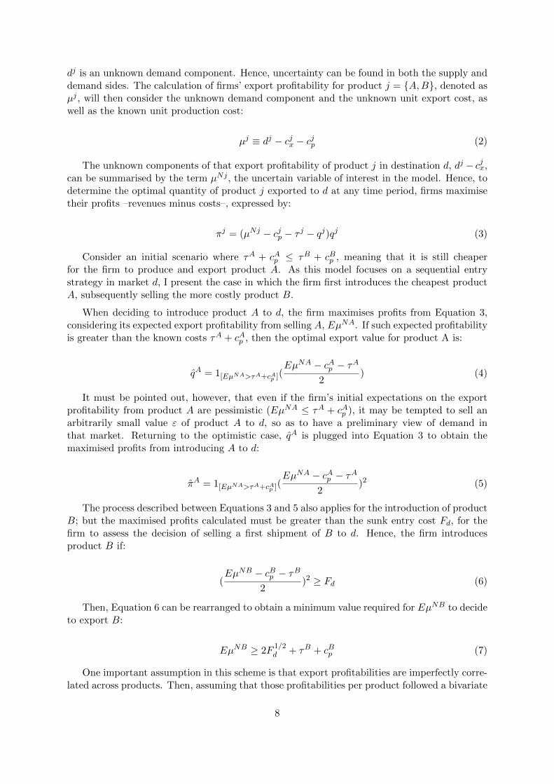
dj is an unknown demand component. Hence, uncertainty can be found in both the supply anddemand sides. The calculation of firms’ export profitability for product j = {A,B}, denoted asµj , will then consider the unknown demand component and the unknown unit export cost, aswell as the known unit production cost:

µj ≡ dj − cjx − cjp (2)

The unknown components of that export profitability of product j in destination d, dj − cjx,can be summarised by the term µNj , the uncertain variable of interest in the model. Hence, todetermine the optimal quantity of product j exported to d at any time period, firms maximisetheir profits –revenues minus costs–, expressed by:

πj = (µNj − cjp − τ j − qj)qj (3)

Consider an initial scenario where τA + cAp ≤ τB + cBp , meaning that it is still cheaperfor the firm to produce and export product A. As this model focuses on a sequential entrystrategy in market d, I present the case in which the firm first introduces the cheapest productA, subsequently selling the more costly product B.

When deciding to introduce product A to d, the firm maximises profits from Equation 3,considering its expected export profitability from selling A, EµNA. If such expected profitabilityis greater than the known costs τA + cAp , then the optimal export value for product A is:

qA = 1[EµNA>τA+cAp ](EµNA − cAp − τA

2) (4)

It must be pointed out, however, that even if the firm’s initial expectations on the exportprofitability from product A are pessimistic (EµNA ≤ τA + cAp ), it may be tempted to sell anarbitrarily small value ε of product A to d, so as to have a preliminary view of demand inthat market. Returning to the optimistic case, qA is plugged into Equation 3 to obtain themaximised profits from introducing A to d:

πA = 1[EµNA>τA+cAp ](EµNA − cAp − τA

2)2 (5)

The process described between Equations 3 and 5 also applies for the introduction of productB; but the maximised profits calculated must be greater than the sunk entry cost Fd, for thefirm to assess the decision of selling a first shipment of B to d. Hence, the firm introducesproduct B if:

(EµNB − cBp − τB

2)2 ≥ Fd (6)

Then, Equation 6 can be rearranged to obtain a minimum value required for EµNB to decideto export B:

EµNB ≥ 2F1/2d + τB + cBp (7)

One important assumption in this scheme is that export profitabilities are imperfectly corre-lated across products. Then, assuming that those profitabilities per product followed a bivariate

8

normal distribution, with parameters (EµNA, EµNB, σA, σB, ρ), I obtain a function for the ex-pected export profitability for B, given the realisation of A:

E(µNB | µNA) = EµNB + (µNA − EµNA)ρσA

σB(8)

This outcome implies that E(µNB | µNA) ≥ 2F1/2d +τB +cBp for the firm to decide to export

B. From Equation 8, I could find a cutoff value of µNA above which the sequential exportingstrategy would be undertaken.

However, under the scheme outlined so far, the firm only needs to make one shipment ofproduct A to automatically realise the export profitability of that product, and that single pieceof information is sufficient to decide whether to export B or not in the next period.

It is pertinent then to consider the more realistic assumption that firm i requires furthershipments to be more certain about the demand of product A in market d. That will not onlyprovide a better view of the demand for A; but will also give a tool to update firm i’s expectedexport profitability of product B, leading to a more backed export decision. Furthermore, tosimplify the model, I propose to take the uncertain export profitability as solely a function ofthe unknown demand of product j from destination d, denoted as xj .6

The maths and notation presented hereafter are inspired from Nguyen (2012), on delaysin the export decision across destinations. Every shipment of product A provides one piece ofinformation on the demand of that good, meaning that the firm is gradually realising the actualdemand of A in market d. However, with those shipments, the firm is updating its expected de-mand of product B. I may propose that each shipment of A produces one perceived demand xAi .All these perceived demands may be gathered in one random vector xA ≡ [xA1 , . . . , x

Aj , . . . , x

AJ ],

where J is an arbitrarily large number of possible shipments.

I assume that demands for A and B in market d (xA and xB) follow a joint bivariatedistribution. If the firm has not entered d yet, the moments of those demands collapse to:

E[xA] = E[xB] = 0 (9a)

V ar[xA] = V ar[xB] = σ20 > 0 (9b)

Cov(xA, xB)

σ20= ρ→ 0 < ρ < 1 (9c)

While the firm begins exporting the less costly product A, it will be gradually updatingits realised demand by calculating the mean demand of that product, considering IA⊂J , thenumber of shipments so far:

xA =Σi∈IAx

Ai

IA(10)

However, when it comes to decide to export product B to market d, the expected value andvariance of the demand on that product are updated in function of the number of shipments of

6The latter implies assuming that the unknown unit export cost cjx to be negligible.

9

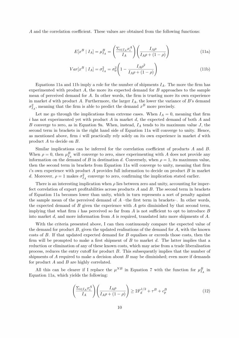
A and the correlation coefficient. These values are obtained from the following functions:

E[xB | IA] = µBIA =

(Σi∈IAx

Ai

IA

)(IAρ

IAρ+ (1− ρ)

)(11a)

V ar[xB | IA] = σ2IA = σ20

(1− IAρ

2

IAρ+ (1− ρ)

)(11b)

Equations 11a and 11b imply a role for the number of shipments IA. The more the firm hasexperimented with product A, the more its expected demand for B approaches to the samplemean of perceived demand for A. In other words, the firm is trusting more its own experiencein market d with product A. Furthermore, the larger IA, the lower the variance of B’s demandσ2IA , meaning that the firm is able to predict the demand xB more precisely.

Let me go through the implications from extreme cases. When IA = 0, meaning that firmi has not experimented yet with product A in market d, the expected demand of both A andB converge to zero, as in Equation 9a. When, instead, IA tends to its maximum value J , thesecond term in brackets in the right hand side of Equation 11a will converge to unity. Hence,as mentioned above, firm i will practically rely solely on its own experience in market d withproduct A to decide on B.

Similar implications can be inferred for the correlation coefficient of products A and B.When ρ = 0, then µBIA will converge to zero, since experimenting with A does not provide anyinformation on the demand of B in destination d. Conversely, when ρ = 1, its maximum value,then the second term in brackets from Equation 11a will converge to unity, meaning that firmi’s own experience with product A provides full information to decide on product B in marketd. Moreover, ρ = 1 makes σ2IA converge to zero, confirming the implication stated earlier.

There is an interesting implication when ρ lies between zero and unity, accounting for imper-fect correlation of export profitabilities across products A and B. The second term in bracketsof Equation 11a becomes lower than unity, which in turn represents a sort of penalty againstthe sample mean of the perceived demand of A –the first term in brackets–. In other words,the expected demand of B given the experience with A gets diminished by that second term,implying that what firm i has perceived so far from A is not sufficient to opt to introduce Binto market d, and more information from A is required, translated into more shipments of A.

With the criteria presented above, I can then continuously compare the expected value ofthe demand for product B, given the updated realisations of the demand for A, with the knowncosts of B. If that updated expected demand for B equalises or exceeds those costs, then thefirm will be prompted to make a first shipment of B to market d. The latter implies that areduction or elimination of any of these known costs, which may arise from a trade liberalisationprocess, reduces the entry cutoff for product B. This subsequently implies that the number ofshipments of A required to make a decision about B may be diminished; even more if demandsfor product A and B are highly correlated.

All this can be clearer if I replace the µNB in Equation 7 with the function for µBIA inEquation 11a, which yields the following:

(Σi∈IAx

Ai

IA

)(IAρ

IAρ+ (1− ρ)

)≥ 2F

1/2d + τB + cBp (12)

10

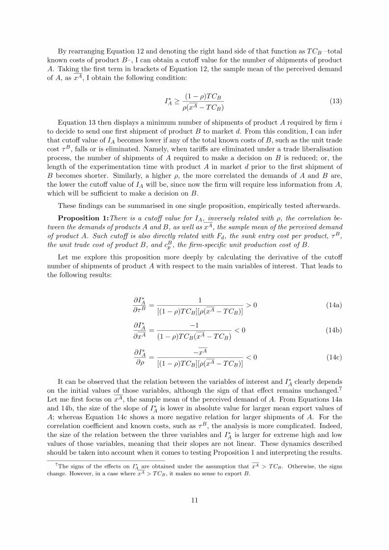
By rearranging Equation 12 and denoting the right hand side of that function as TCB –totalknown costs of product B–, I can obtain a cutoff value for the number of shipments of productA. Taking the first term in brackets of Equation 12, the sample mean of the perceived demandof A, as xA, I obtain the following condition:

I∗A ≥(1− ρ)TCB

ρ(xA − TCB)(13)

Equation 13 then displays a minimum number of shipments of product A required by firm ito decide to send one first shipment of product B to market d. From this condition, I can inferthat cutoff value of IA becomes lower if any of the total known costs of B, such as the unit tradecost τB, falls or is eliminated. Namely, when tariffs are eliminated under a trade liberalisationprocess, the number of shipments of A required to make a decision on B is reduced; or, thelength of the experimentation time with product A in market d prior to the first shipment ofB becomes shorter. Similarly, a higher ρ, the more correlated the demands of A and B are,the lower the cutoff value of IA will be, since now the firm will require less information from A,which will be sufficient to make a decision on B.

These findings can be summarised in one single proposition, empirically tested afterwards.

Proposition 1:There is a cutoff value for IA, inversely related with ρ, the correlation be-tween the demands of products A and B, as well as xA, the sample mean of the perceived demandof product A. Such cutoff is also directly related with Fd, the sunk entry cost per product, τB,the unit trade cost of product B, and cBp , the firm-specific unit production cost of B.

Let me explore this proposition more deeply by calculating the derivative of the cutoffnumber of shipments of product A with respect to the main variables of interest. That leads tothe following results:

∂I∗A∂τB

=1

[(1− ρ)TCB][ρ(xA − TCB)]> 0 (14a)

∂I∗A

∂xA=

−1

(1− ρ)TCB(xA − TCB)< 0 (14b)

∂I∗A∂ρ

=−xA

[(1− ρ)TCB][ρ(xA − TCB)]< 0 (14c)

It can be observed that the relation between the variables of interest and I∗A clearly dependson the initial values of those variables, although the sign of that effect remains unchanged.7

Let me first focus on xA, the sample mean of the perceived demand of A. From Equations 14aand 14b, the size of the slope of I∗A is lower in absolute value for larger mean export values ofA; whereas Equation 14c shows a more negative relation for larger shipments of A. For thecorrelation coefficient and known costs, such as τB, the analysis is more complicated. Indeed,the size of the relation between the three variables and I∗A is larger for extreme high and lowvalues of those variables, meaning that their slopes are not linear. These dynamics describedshould be taken into account when it comes to testing Proposition 1 and interpreting the results.

7The signs of the effects on I∗A are obtained under the assumption that xA > TCB . Otherwise, the signschange. However, in a case where xA > TCB , it makes no sense to export B.

11

Given the data availability, I may test the effect of trade liberalisation, as a tariff eliminationby country d on most products, on the number of shipments by firm i of old products prior tothe first shipments of a new product to market d. The number of shipments may also be proxiedby the length of the time spell between the first shipment of product A and the equivalent ofproduct B. The data also allows me to measure the impact of the mean export value of productA before the first shipment of B, as a proxy for the perceived demand of A in market d.

4 Data and Summary Statistics

4.1 The Data

The export data was provided by the Peruvian Society of Foreign Trade (COMEXPERU inSpanish), which manages data on daily export and import transactions from diverse sectors.This information is collected from the Peruvian Tax and Tariff Agency (Superintendencia Na-cional de Administracion Tributaria - SUNAT in Spanish).

The original datasets range from 1998 to 2013, each compiling information on daily exporttransactions per firm, from eight sectors: Agriculture, Basic Metal Industries, Chemical, Jew-ellery, Metallic-Mechanics, Non-Metallic Mining, Textile and Apparel, and Timber and Paper.

Each transaction contains very detailed information, such as the transaction date, nameand tax code of the firm, port of departure, description and 10-digit tariff line of the product,destination and port of arrival, export value in US dollars, weight and unit of measure. Thispaper focuses on manufacturing industries due to the large share of small firms comprised,unlike more traditional extractive industries dominated by medium and large firms, as well asthe known previous controversy on a potential damage by an FTA with the US to Peruvianmanufacturers, especially the smallest firms.

From the Peruvian Tax and Tariff Agency, I also collected firm-level information, such asthe year each firm came into existence and, where relevant, the year they exited the business,as well as the region their main headquarters is located.

Aiming to account for trade liberalisation, I collected the tariff rates levied by the UnitedStates at the HS 8-digit level, from the World Integrated Trade Solutions (WITS) database ofthe World Bank. These tariff rates derive from the Most Favoured Nation (MFN) scheme, until2008. From 2009 onwards, under the Free Trade Agreement (FTA) between Peru and USA, thevast majority of these tariff rates become zero. Since many products were unilaterally liberalisedby the US before the enactment of the FTA under the ATPDEA scheme, I also obtained thelist of 8-digit tariff lines eligible under that regime, with their respective tariff until 2008.

For this analysis, I converted the original exports dataset into one on a daily basis. Thus, Iproceeded to construct observations at the firm/day level, each representing one day on whichfirm i exports one or a set of new products to USA. This process involved the generation ofrelevant information, such as the number of days elapsing between rounds of new exports; everyexact date each round took place, as well as the number of new products introduced and theorder in which these new products were exported to USA for the first time.

This resulting daily dataset of new exports, covering the 2006-2013 period, is restricted tofirms that started their business since 2006, leading to a total of 2,426 firms that sold to USA.This final sample does not distinguish between firms starting to export to USA with one singleproducts and those starting with more than one good. It also considers those firms that neverexported to USA up to three years since founded, which raises the number to 7,806 firms.

12

4.2 Summary Statistics

4.2.1 Firms and Rounds of New Exports

Table 1 displays the 7,806 firms considered, according to their year of foundation, regardlessof whether they ever exported or not to USA. In some statistics, I distinguish between firmsstarting before (pre− FTAfirms) and from 2009 (post− FTAfirms), intending to identify apotential influence of the USA-Peru FTA on firms’ experimentation decisions. Hence, I end upwith approximately 60% of firms that are post− FTA.

Table 1: Peru-USA - Exporters per Starting Year 2006-2013

Year Freq. Percent Cum.

2006 1009 12.93 12.932007 992 12.71 25.632008 1052 13.48 39.112009 1149 14.72 53.832010 1044 13.37 67.22011 1055 13.52 80.722012 973 12.46 93.182013 532 6.82 100

Total 7806 100

Source: COMEXPERU - SUNAT

From the eight sectors mentioned above, clearly Agriculture and Textile and Apparel arethose accounting for the largest amount of firm export transactions involving new products –experimentation rounds–. Hence, for further analyses I gather the six remaining sectors into thegroup “OTHERS”. Table 2 groups the experimentation rounds according to the sector productj belongs to. The upper part considers only the first experimentation round by each of the2,426 firms that ever exported to USA; whereas the lower part includes all rounds registered,leading to a total of 7,532 experimentation rounds by those 2,426 firms. 8

8Products sold in one round may belong to more than one sector. However, the raw daily data shows thatproducts from secondary sectors are mostly sold at minimum values compared to firms’ core sectors. Also, thegrouping made, which considers non-agriculture and non-textile exports into one category, helps control for thisissue, assuming that one round of new exports consists of products from only one of these three groups.

13

Table 2: Peru-USA - Exporters per Sector 2006-2013

Sector (firstexports)

Freq. Percent Cum.

Agriculture 792 32.65 32.65Textile-Apparel 789 32.52 65.17Others 845 34.83 100

Total 2426 100

Sector (allnew exports)

Freq. Percent Cum.

Agriculture 1782 23.66 23.66Textile-Apparel 3624 48.11 71.77Others 2126 28.23 100

Total 7532 100

Source: COMEXPERU - SUNAT

Although the focus is the US market, it is also relevant to take into account firms’ experiencein other destinations. Nevertheless, the daily basis and the nature of my dataset make itmore difficult to control for that experience. As an approximation, I constructed the dummyelsewhere, taking value 1 if, in the latest month I have information from firm i prior to itsexperimentation round in USA analysed, that firm exported to any other destination. In Table3 I distinguish the new export rounds according to that criterion, and it is evident from firstexperimentation rounds in USA that most Peruvian firms have one previous experience inother markets, presumably neighbouring countries like those from the Andean Community andMERCOSUR. However, as firms subsequently experiment with more products in USA, it seemsthey become more focused in that destination, as results for all new exports show.

Table 3: Peru-USA - Exporters to USA Only vs. Elsewhere 2006-2013

Elsewhere(first exports)

Freq. Percent Cum.

No 298 12.28 12.28Yes 2128 87.72 100

Total 2426 100

Elsewhere (allnew exports)

Freq. Percent Cum.

No 3534 46.92 46.92Yes 3998 53.08 100

Total 7532 100

Source: COMEXPERU - SUNAT

14

4.2.2 Number of Products Exported

The following tables are more concentrated on the number of products exported by Peruvian firmi to USA. Table 4 groups firms according to the maximum number of new products introducedby firms in one single experimentation round. The figures show that most firms in the sample(55.15%) experiment with only one new product per attempt, followed by a 14.88% of firmsexporting up to two new products in a round.

Table 4: Peru-USA - Maximum Number of New ProductsIntroduced by Firm i to USA on Day t 2006-2013

N◦ Freq. Percent Cum.

1 1338 55.15 55.152 361 14.88 70.033 187 7.71 77.744 138 5.69 83.435 93 3.83 87.266 74 3.05 90.317 60 2.47 92.798 32 1.32 94.119 33 1.36 95.4710 22 0.91 96.3711 - 20 65 2.65 99.0221 - 94 23 0.92 100

Total 2426 100

Source: COMEXPERU - SUNAT

It is equally striking to find that, throughout the 2006-2013 period, slightly more than 40%of firms have only exported one product to USA in total, as Table 5 states. Indeed, more thana half of the 2,426 firms that exported to USA during that period, have only introduced up totwo products into that market.

To have a clearer view of firms’ performance in terms of product experimentation in USA,in Table 6 I take all the 7,532 experimentation rounds counted to see how many productsthese rounds comprise. As expected from the previous numbers, over 64% of these rounds arecomposed by only one new product.

15

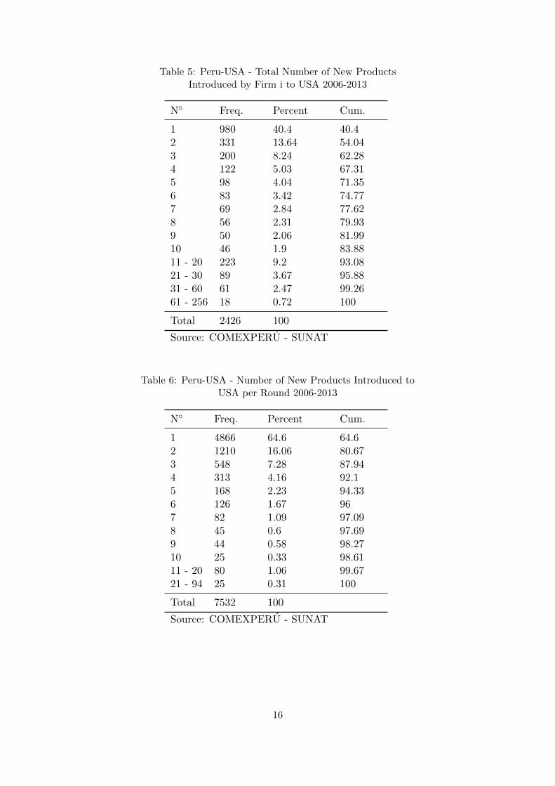
Table 5: Peru-USA - Total Number of New ProductsIntroduced by Firm i to USA 2006-2013

N◦ Freq. Percent Cum.

1 980 40.4 40.42 331 13.64 54.043 200 8.24 62.284 122 5.03 67.315 98 4.04 71.356 83 3.42 74.777 69 2.84 77.628 56 2.31 79.939 50 2.06 81.9910 46 1.9 83.8811 - 20 223 9.2 93.0821 - 30 89 3.67 95.8831 - 60 61 2.47 99.2661 - 256 18 0.72 100

Total 2426 100

Source: COMEXPERU - SUNAT

Table 6: Peru-USA - Number of New Products Introduced toUSA per Round 2006-2013

N◦ Freq. Percent Cum.

1 4866 64.6 64.62 1210 16.06 80.673 548 7.28 87.944 313 4.16 92.15 168 2.23 94.336 126 1.67 967 82 1.09 97.098 45 0.6 97.699 44 0.58 98.2710 25 0.33 98.6111 - 20 80 1.06 99.6721 - 94 25 0.31 100

Total 7532 100

Source: COMEXPERU - SUNAT

16

4.2.3 Experimentation Rounds per Firm

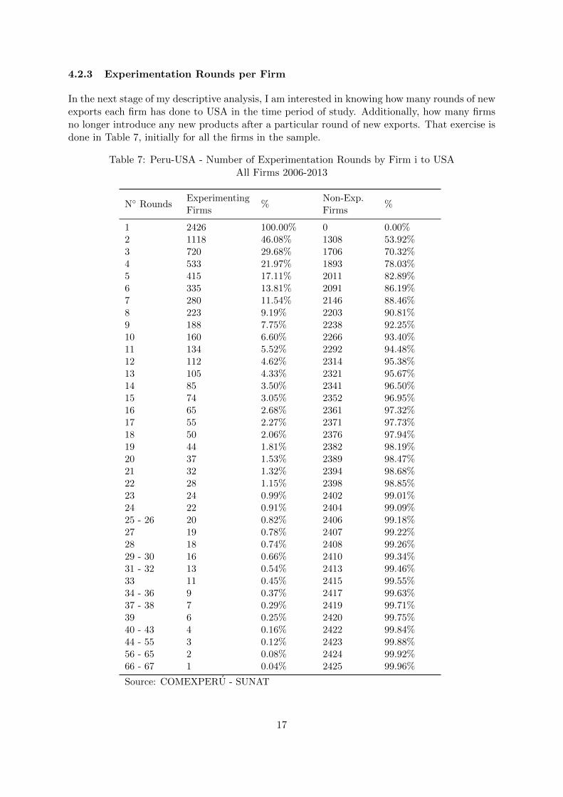
In the next stage of my descriptive analysis, I am interested in knowing how many rounds of newexports each firm has done to USA in the time period of study. Additionally, how many firmsno longer introduce any new products after a particular round of new exports. That exercise isdone in Table 7, initially for all the firms in the sample.

Table 7: Peru-USA - Number of Experimentation Rounds by Firm i to USAAll Firms 2006-2013

N◦ RoundsExperimentingFirms

%Non-Exp.Firms

%

1 2426 100.00% 0 0.00%2 1118 46.08% 1308 53.92%3 720 29.68% 1706 70.32%4 533 21.97% 1893 78.03%5 415 17.11% 2011 82.89%6 335 13.81% 2091 86.19%7 280 11.54% 2146 88.46%8 223 9.19% 2203 90.81%9 188 7.75% 2238 92.25%10 160 6.60% 2266 93.40%11 134 5.52% 2292 94.48%12 112 4.62% 2314 95.38%13 105 4.33% 2321 95.67%14 85 3.50% 2341 96.50%15 74 3.05% 2352 96.95%16 65 2.68% 2361 97.32%17 55 2.27% 2371 97.73%18 50 2.06% 2376 97.94%19 44 1.81% 2382 98.19%20 37 1.53% 2389 98.47%21 32 1.32% 2394 98.68%22 28 1.15% 2398 98.85%23 24 0.99% 2402 99.01%24 22 0.91% 2404 99.09%25 - 26 20 0.82% 2406 99.18%27 19 0.78% 2407 99.22%28 18 0.74% 2408 99.26%29 - 30 16 0.66% 2410 99.34%31 - 32 13 0.54% 2413 99.46%33 11 0.45% 2415 99.55%34 - 36 9 0.37% 2417 99.63%37 - 38 7 0.29% 2419 99.71%39 6 0.25% 2420 99.75%40 - 43 4 0.16% 2422 99.84%44 - 55 3 0.12% 2423 99.88%56 - 65 2 0.08% 2424 99.92%66 - 67 1 0.04% 2425 99.96%

Source: COMEXPERU - SUNAT

17

The way to read these results is as follows: from the 2,426 firms that exported one first setof new products to USA, 1,118 firms (46.08%) move one step forward, undertaking a secondexperimentation round; while the other 1,308 (53.92%) firms never experimented with anothernew product again. Hence, for the effects of the survival analysis made afterwards, those 1,308firms are considered as right censored. In a similar way, the next rows can be interpreted, sothat only one firm managed to have up to 67 experimentation rounds; leaving the other 2,425firms as right censored.

For the sake of that survival analysis, it is also necessary to establish differences in perfor-mance between pre− FTA and post− FTA firms. Hence, under the same previous rationale,Table 8 presents the equivalent exercise separately for both types of firms. It can be found thatthe level of experimentation and right censoring across the two groups is very similar. Indeed,45.47% of pre− FTA firms jumped from the first to the second experimentation round; whilethat was the case for 46.71% of post−FTA firms. Figures remain similar across the subsequentrounds, with the exception that the most experimenting post−FTA firm has come to 39 roundsof new products, compared to the 67 rounds of one pre− FTA firm.

18

Table 8: Peru-USA - Number of Experimentation Rounds by Firm i to USA

(a) Pre-FTA Firms 2006-2008

N◦

RoundsExperimentingFirms

%Non-Exp.Firms

%

1 1225 100.00% 0 0.00%2 557 45.47% 668 54.53%3 360 29.39% 865 70.61%4 273 22.29% 952 77.71%5 214 17.47% 1011 82.53%6 174 14.20% 1051 85.80%7 145 11.84% 1080 88.16%8 112 9.14% 1113 90.86%9 100 8.16% 1125 91.84%10 88 7.18% 1137 92.82%11 76 6.20% 1149 93.80%12 65 5.31% 1160 94.69%13 64 5.22% 1161 94.78%14 54 4.41% 1171 95.59%15 45 3.67% 1180 96.33%16 39 3.18% 1186 96.82%17 35 2.86% 1190 97.14%18 31 2.53% 1194 97.47%19 28 2.29% 1197 97.71%20 25 2.04% 1200 97.96%21 22 1.80% 1203 98.20%22 20 1.63% 1205 98.37%23 17 1.39% 1208 98.61%24 16 1.31% 1209 98.69%25 - 26 14 1.14% 1211 98.86%27 13 1.06% 1212 98.94%28 12 0.98% 1213 99.02%29- 30 11 0.90% 1214 99.10%31- 33 10 0.82% 1215 99.18%34- 36 8 0.65% 1217 99.35%37 - 38 6 0.49% 1219 99.51%39 5 0.41% 1220 99.59%40 - 43 4 0.33% 1221 99.67%44 - 55 3 0.24% 1222 99.76%56 - 65 2 0.16% 1223 99.84%66 - 67 1 0.08% 1224 99.92%

Source: COMEXPERU - SUNAT

(b) Post-FTA firms 2009-2013

N◦

RoundsExperimentingFirms

%Non-Exp.Firms

%

1 1201 100.00% 0 0.00%2 561 46.71% 640 53.29%3 360 29.98% 841 70.02%4 260 21.65% 941 78.35%5 201 16.74% 1000 83.26%6 161 13.41% 1040 86.59%7 135 11.24% 1066 88.76%8 111 9.24% 1090 90.76%9 88 7.33% 1113 92.67%10 72 6.00% 1129 94.00%11 58 4.83% 1143 95.17%12 47 3.91% 1154 96.09%13 41 3.41% 1160 96.59%14 31 2.58% 1170 97.42%15 29 2.41% 1172 97.59%16 26 2.16% 1175 97.84%17 20 1.67% 1181 98.33%18 19 1.58% 1182 98.42%19 16 1.33% 1185 98.67%20 12 1.00% 1189 99.00%21 10 0.83% 1191 99.17%22 8 0.67% 1193 99.33%23 7 0.58% 1194 99.42%24- 28 6 0.50% 1195 99.50%29- 30 5 0.42% 1196 99.58%31- 32 3 0.25% 1198 99.75%33- 39 1 0.08% 1200 99.92%

Source: COMEXPERU - SUNAT

19

4.2.4 Export Values and Preference Regimes

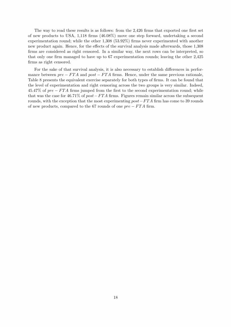
It should always be regarded that, prior to the enactment of the USA-Peru Free Trade Agree-ment, several Peruvian products had a tariff-free access to the US market by unilateral tradepreferences from that country, under the ATPDEA and zero-MFN schemes. The next two ta-bles group the rounds of new exports according to whether they include at least one productfavoured by either of those regimes. Table 9 covers all the 7,532 experimentation rounds in thesample; while Table 10 exclusively focuses on the first exports by each of the 2,426 firms.

The figures in Table 9 reveal that, in my whole sample, 51.35% of experimentation roundsby firms include at least one product that was affected by one of the aforementioned regimesbefore the FTA was effective. That share is much larger for first exports only as shown in Table10. 63.27% of firms in the sample have started their experience in the US market with either anATPDEA or zero-MFN product. However, the amount of experimentation rounds comprisingonly products with no pre-FTA unilateral trade preference is also remarkable.

Table 9: Peru-USA - New Exports to USA per Preference Regime 2006-2013

At least one new ATPDEAproduct to USA on day t

At least one new MFN product toUSA on day t

No Yes Total

No 3664 1206 4870Yes 1622 1040 2662

Total 5286 2246 7532

Source: WITS - World Bank

Table 10: Peru-USA - First Exports to USA per Preference Regime 2006-2013

New ATPDEA productto USA on day t

New MFN product to USA onday t

No Yes Total

No 891 534 1425Yes 668 333 1001

Total 1559 867 2426

Source: WITS - World Bank

Briefly looking at daily exports by Peruvian firms to USA during 2006-2013, I constructedsome Kernel densities of the log of total exports by firm i to that market on day t, consideringonly those days in which firms undertook an experimentation round, also taking into accountthat in those days –except for the first exports– firms may have exported both new productsand other goods the firm previously exported to USA. Figures 1 and 2 display those densitiesfor all the 7,532 experimentation rounds in the sample, and only the 2,426 first new exports,respectively. This is one of the first exercises aiming at distinguishing between firms activebefore and after the enactment of the FTA, and it shows that export values by post − FTAfirms tend to be larger than those by older firms. Furthermore, focusing on Figure 2, the initialvalue with which post−FTA firms jump into the US market is usually larger than for pre−FTAfirms. While the latter on average start with a US $ 21,568.26 shipment, the former do it witha mean value of US $ 28,530.08.

20

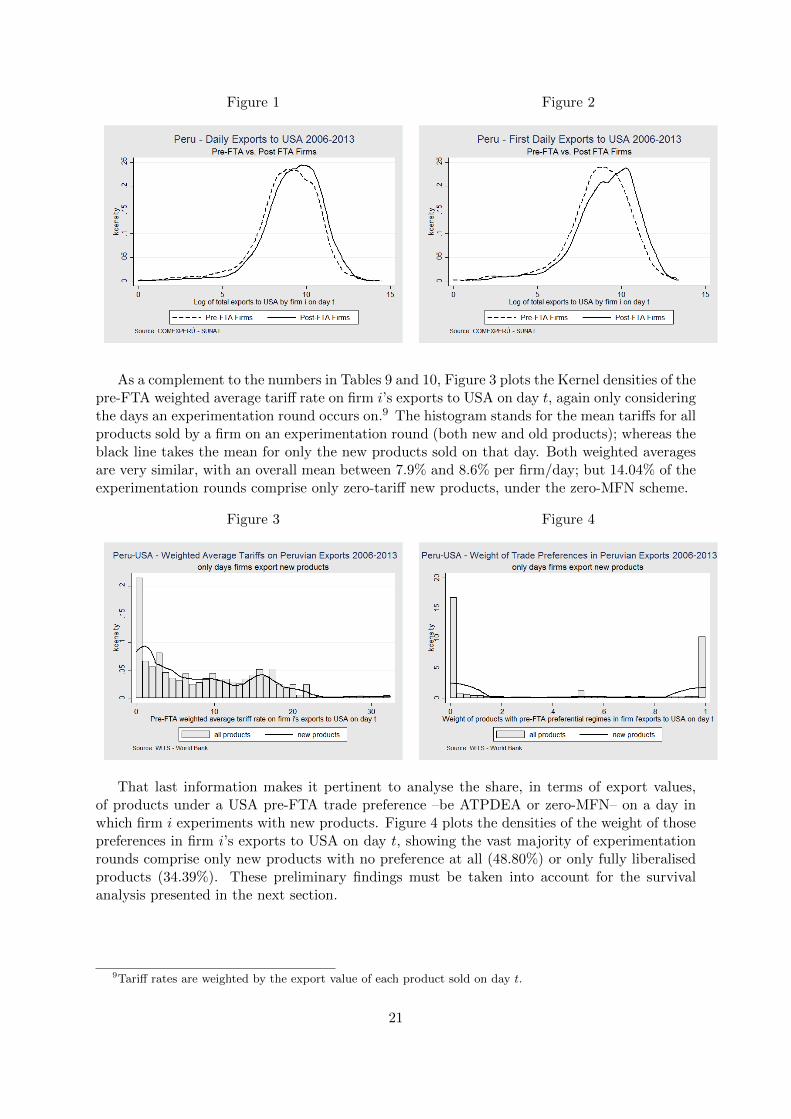
Figure 1 Figure 2

As a complement to the numbers in Tables 9 and 10, Figure 3 plots the Kernel densities of thepre-FTA weighted average tariff rate on firm i’s exports to USA on day t, again only consideringthe days an experimentation round occurs on.9 The histogram stands for the mean tariffs for allproducts sold by a firm on an experimentation round (both new and old products); whereas theblack line takes the mean for only the new products sold on that day. Both weighted averagesare very similar, with an overall mean between 7.9% and 8.6% per firm/day; but 14.04% of theexperimentation rounds comprise only zero-tariff new products, under the zero-MFN scheme.

Figure 3 Figure 4

That last information makes it pertinent to analyse the share, in terms of export values,of products under a USA pre-FTA trade preference –be ATPDEA or zero-MFN– on a day inwhich firm i experiments with new products. Figure 4 plots the densities of the weight of thosepreferences in firm i’s exports to USA on day t, showing the vast majority of experimentationrounds comprise only new products with no preference at all (48.80%) or only fully liberalisedproducts (34.39%). These preliminary findings must be taken into account for the survivalanalysis presented in the next section.

9Tariff rates are weighted by the export value of each product sold on day t.

21

5 Survival Analysis

My main interest is to test the main prediction from my theoretical model, finding whether tradeliberalisation, in the shape of the tariff elimination on Peruvian goods exported to USA under the2009 Free Trade Agreement, plays a facilitating role for experimentation. I am also interested inassessing a potential role of the size of export shipments prior to firms’ experimentation rounds.One convenient approach is to characterise how long it takes for a Peruvian firm to introduceone or more new products into the USA market; namely, Peruvian firms’ experimentation speedin that destination; and the main determinants of that speed.

To attain that outcome, I undertook a survival analysis which calculates the well-knownKaplan-Meier Survival Function. The innovation in this analysis, as opposed to most studiesthat consider as a failure the event of a firm leaving an export market or even dropping out ofthe export activity, is that the “failure” I assess is the event in which a Peruvian firm sells oneor many new products to the US market, i.e. the occurrence of an experimentation round. Itshould be kept in mind that a product is taken as “new” at the firm-destination level. That is,a product is new if firm i has never exported it to USA before.

Econometrics textbooks like Cleves et al. (2010) report that the Kaplan-Meier Estimator isa nonparametric estimate of the survival function, denoted as S(t). That estimate, also knownas the product limit estimate of S(t) at any time t is defined as:

S(t) = Πj|tj≤t(nj − djnj

) (15)

where nj is the number of observations at risk at time tj , and dj is the number of failures atsuch tj . This function is a product considering all j times there is a failure, both before andat time t. As a result, the estimate of the failure function is the supplement of the estimatedsurvival function: 1− S(t).

The basic way to interpret the Kaplan-Meier Estimator is: at day t, what is the probabilityfor firms to introduce one or more new products into USA (failure)? Alternatively, at day t,what is the probability for firms to no longer experiment in USA with any other new product(survival)? The time span is measured in days, depending on the order of the experimentationround. For instance, for the first new exports by firm i to USA, I count the number of days sincefirm i was established. For the second experimentation round, in contrast, I count how manydays have elapsed since firm i’s first products sold to USA. That latter rationale is applied forthe subsequent rounds. Note that the analysis considers the right censored firms lost in eachround, as well as those that never exported to USA during the 2006-2013 period.

5.1 Pre-FTA vs. Post-FTA Firms

For the first Kaplan-Meier analysis, I split the sample of 7,806 firms according to their year offoundation, leading to 3,053 firms starting between 2006 and 2008 –pre−FTA firms– and 4,753founded between 2009 and 2013 –post− FTA firms–. The outcomes are striking.

Figure 5 provides an overall comparison of the Kaplan-Meier Survival Function between bothtypes of firms, considering the pool of experimentation rounds, regardless of the order and thefirm. The observations ”at risk” in this exercise are the number of days elapsed since the previousexperimentation round of firm i. The dashed line shows the function for the experimentationrounds by pre− FTA firms; whereas the solid line is the equivalent for post− FTA firms.

22

This figure shows that, overall, experimentation rounds by pre − FTA firms take shorterto effectively occur than by post − FTA firms. More precisely, this outcome tells that theprobability for pre− FTA firms of introducing one or many new products into the US marketrises to 50% 423 days after their previous experimentation round; while that probability isreached at 646 days for post − FTA firms. Similarly, the ”failure” probability became 25% at79 days for pre − FTA firms; while for post − FTA firms, that likelihood was reached at 95days. This might indicate that pre − FTA firms tend to experiment faster than post − FTAfirms; however, after 1,500 days approximately, the survival probability for post − FTA firmsbecomes lower. This is likely to be explained by the longer existence of pre− FTA firms. Theresults also indicate that, after 1,718 days, there is one time spell by a post − FTA firm thatdoes not end up with a new experimentation round, leading to a final survival probability of2.86%. As for pre−FTA firms, the survival probability becomes zero after 2,862 days, meaningthat all the time spells ”at risk” concluded with the introduction of a new product into the USmarket, with many other time spells becoming right-censored in between.10

Figure 5

However, I consider it much more informative to estimate the survival probability separatelyfor each experimentation round, so that the interpretation can be done at the firm level. Thus,Figure 6 presents the results for each of the first four rounds of new exports. The patternobserved in Figure 5 is somehow exhibited in Figure 6a) for the first experimentation rounds byfirms. This time, both estimates of the survival function follow the same path; but the survivalprobability for post−FTA firms drops at a larger pace from day 1,424. For post−FTA firms,the probability of experimenting for the first time in USA becomes 50% at 1,419 days since thefirm was founded; while that length was 1,391 days for pre−FTA firms. For the reason exposedearlier, the survival probability becomes zero –the probability of exporting for the first time toUSA becomes one– after 1,682 days for post−FTA firms and 2,862 days for pre−FTA firms.

10A time spell becomes right-censored if a firm never exports to USA or does no longer sell any other newproduct to USA. The date considered to close that time spell is either the day the firm closed down or the lastdate the firm sold any product to any other destination in my sample.

23

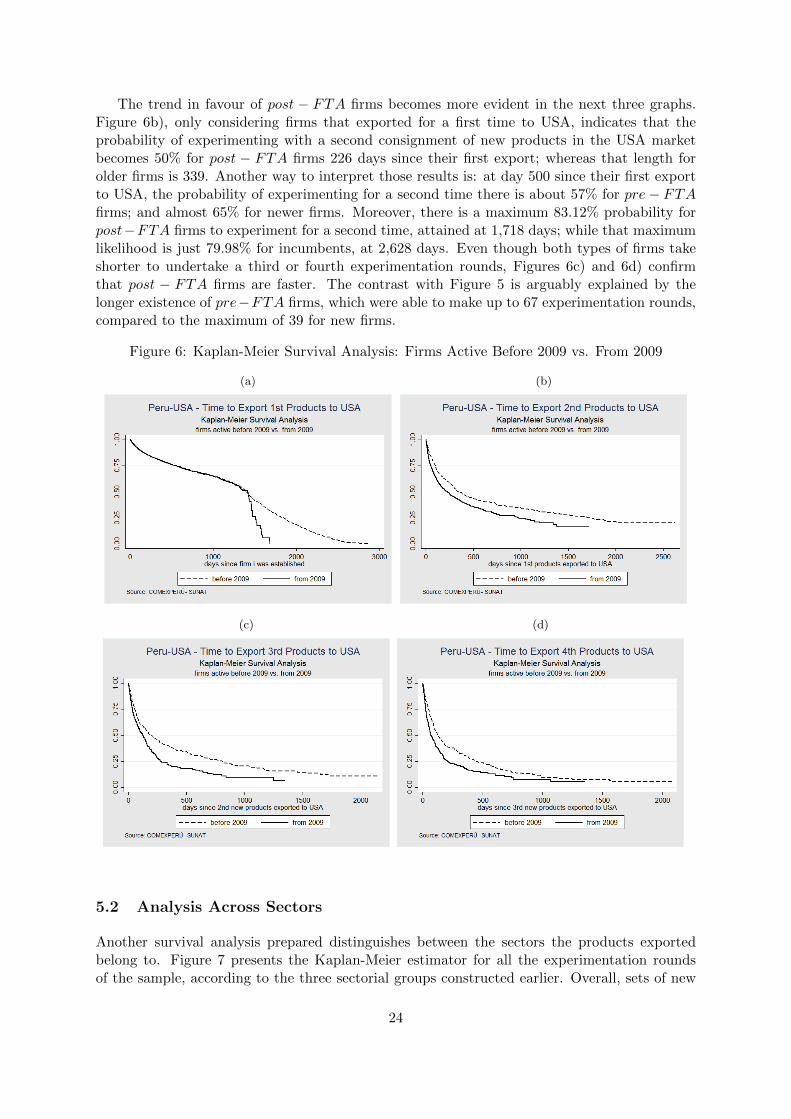
The trend in favour of post − FTA firms becomes more evident in the next three graphs.Figure 6b), only considering firms that exported for a first time to USA, indicates that theprobability of experimenting with a second consignment of new products in the USA marketbecomes 50% for post − FTA firms 226 days since their first export; whereas that length forolder firms is 339. Another way to interpret those results is: at day 500 since their first exportto USA, the probability of experimenting for a second time there is about 57% for pre− FTAfirms; and almost 65% for newer firms. Moreover, there is a maximum 83.12% probability forpost−FTA firms to experiment for a second time, attained at 1,718 days; while that maximumlikelihood is just 79.98% for incumbents, at 2,628 days. Even though both types of firms takeshorter to undertake a third or fourth experimentation rounds, Figures 6c) and 6d) confirmthat post − FTA firms are faster. The contrast with Figure 5 is arguably explained by thelonger existence of pre−FTA firms, which were able to make up to 67 experimentation rounds,compared to the maximum of 39 for new firms.

Figure 6: Kaplan-Meier Survival Analysis: Firms Active Before 2009 vs. From 2009

(a) (b)

(c) (d)

5.2 Analysis Across Sectors

Another survival analysis prepared distinguishes between the sectors the products exportedbelong to. Figure 7 presents the Kaplan-Meier estimator for all the experimentation roundsof the sample, according to the three sectorial groups constructed earlier. Overall, sets of new

24

exports embracing textile and apparel products –solid line– take place faster than agriculturalexports –dashed line–, as well as other manufacturing industries –dotted line–. Note that, sinceI compare the span lengths between sectors, it is impossible to control for right-censored firmsin this estimation.

Figure 7

When looking at each round separately, Kaplan-Meier estimations –not reported in thispaper– reveal that agricultural first exports tend to be faster than those from other sectors; butfrom the second round onwards, textile and apparel new exports take less days than the rest.

In order to better assess the findings from this exercise, I combined the analysis acrosssectors with the pre-FTA vs. post-FTA criterion. But I consider it more informative to splitthe experimentation rounds by pre − FTA firms between rounds before and after 2009, soas to identify a clearer role of trade liberalisation. Figure 8 presents a set of nine graphswith the results from the criteria combination. The first row shows the overall analysis for allexperimentation rounds; the second one, only the first exports; and the third one, the secondround. The first column considers the new exports by pre − FTA firms done before the 2009FTA; the second column takes those made by such firms since the FTA; and the third one workswith all post− FTA firms.

The dynamics previously described of experimentation across sectors are still evident in thisestimation. What is most remarkable, looking at the second row of first exports, is that theargued faster experimentation speed by agricultural exports is mostly explained by pre-FTAtransactions by pre − FTA firms (Figure 8(d)) and, to a much lesser extent, transactions bypost−FTA firms (Figure 8(f)). In the case of post-FTA transactions by pre−FTA firms (Figure8(e)), it is textile exports that are effective faster, just like in subsequent rounds. This outcomemay imply a particular boost for textile exports by the Free Trade Agreement, especially forfirms that, prior to the FTA, depended on the ATPDEA trade preferences given by USA tomany textile exports, and were not certain about the renewal of those preferences. Also, sometextile products were levied with very high tariffs, meaning that, with the elimination of thosetariffs since 2009, it is much easier to export these products, in a shorter time span.

25

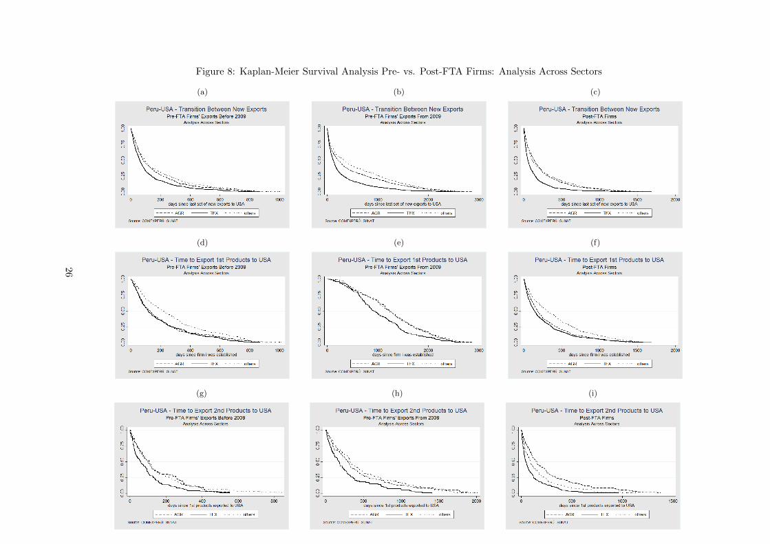
Figure 8: Kaplan-Meier Survival Analysis Pre- vs. Post-FTA Firms: Analysis Across Sectors

(a) (b) (c)

(d) (e) (f)

(g) (h) (i)

26

5.3 Exporting One or Many New Products

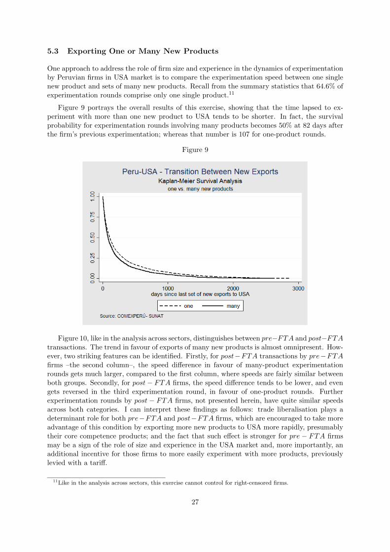
One approach to address the role of firm size and experience in the dynamics of experimentationby Peruvian firms in USA market is to compare the experimentation speed between one singlenew product and sets of many new products. Recall from the summary statistics that 64.6% ofexperimentation rounds comprise only one single product.11

Figure 9 portrays the overall results of this exercise, showing that the time lapsed to ex-periment with more than one new product to USA tends to be shorter. In fact, the survivalprobability for experimentation rounds involving many products becomes 50% at 82 days afterthe firm’s previous experimentation; whereas that number is 107 for one-product rounds.

Figure 9

Figure 10, like in the analysis across sectors, distinguishes between pre−FTA and post−FTAtransactions. The trend in favour of exports of many new products is almost omnipresent. How-ever, two striking features can be identified. Firstly, for post−FTA transactions by pre−FTAfirms –the second column–, the speed difference in favour of many-product experimentationrounds gets much larger, compared to the first column, where speeds are fairly similar betweenboth groups. Secondly, for post− FTA firms, the speed difference tends to be lower, and evengets reversed in the third experimentation round, in favour of one-product rounds. Furtherexperimentation rounds by post − FTA firms, not presented herein, have quite similar speedsacross both categories. I can interpret these findings as follows: trade liberalisation plays adeterminant role for both pre−FTA and post−FTA firms, which are encouraged to take moreadvantage of this condition by exporting more new products to USA more rapidly, presumablytheir core competence products; and the fact that such effect is stronger for pre − FTA firmsmay be a sign of the role of size and experience in the USA market and, more importantly, anadditional incentive for those firms to more easily experiment with more products, previouslylevied with a tariff.

11Like in the analysis across sectors, this exercise cannot control for right-censored firms.

27

Figure 10: Kaplan-Meier Survival Analysis Pre- vs. Post-FTA Firms: One vs. Many Products Exported

(a) (b) (c)

(d) (e) (f)

28

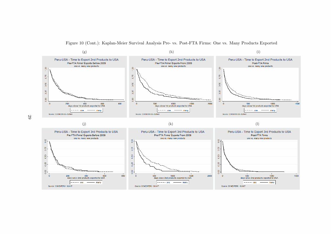
Figure 10 (Cont.): Kaplan-Meier Survival Analysis Pre- vs. Post-FTA Firms: One vs. Many Products Exported

(g) (h) (i)

(j) (k) (l)

29

5.4 Analysis Across Mean Export Values

My theoretical model predicts that the number of shipments of product A by firm i to countryd prior to the introduction of B is inversely correlated with i’s mean export value of shipmentsof A. Thus, I test this prediction with a Kaplan-Meier survival analysis on the experimentationspeed across quintiles of the mean export value of shipments by a Peruvian firm prior to a newexperimentation round in the USA market. The exercise separately utilises shipments to USAonly and to all destinations.

5.4.1 Mean Exports to USA

In this first estimation, I obtain quintiles of the mean values of shipments by firm i to USA, fromits first shipment of product A inclusively, to the last one before the introduction of product B.The same rule applies for all subsequent experimentation rounds. The mean export quintilesare as follows:

• First quintile: mean export value of up to US $ 662.

• Second quintile: above US $ 662 and up to US $ 2,379.

• Third quintile: above US $ 2,379 and up to US $ 6,542.35.

• Fourth quintile: above US $ 6,542.35 and up to US $ 20,625.50.

• Fifth quintile: above US $ 20,625.50.

Each graph elaborated in this analysis shows five step lines, each of them representing oneof the mentioned quintiles.

Figure 11 compiles all experimentation rounds, regardless of the firm; while Figure 12 focuseson the second new products exported to USA per firm. Recall that, since I work with theprevious shipments to USA, the first experimentation rounds are excluded from this exercise.

Figure 11 tells that introductions of new products to USA preceded by small mean shipmentvalues tend to occur quite faster than experimentations following larger mean export values.Thus, for the first quintile function –the solid grey line–, the experimentation probability be-comes 50% at day 56 since last experimentation round. Conversely, for the last quintile function–the solid black line–, that probability is attained at day 254.

Figure 12 on the introduction of the second new products to USA portrays a commonpattern that will be more clearly seen in the forthcoming graphs: there is a growing difference insurvival/failure probabilities between experimentation rounds from the first three quintiles andthe last two, embracing mean exports above US $ 6,542.35. Introduction of second new exportspreceded by average shipments up to US $ 6,542.35 take a shorter span than experimentationrounds occurring after mean exports above that value.

These findings appear to go against the prediction from my theoretical approach. However,looking at differences between pre − FTA and post − FTA transactions may provide furtherinformation.

30

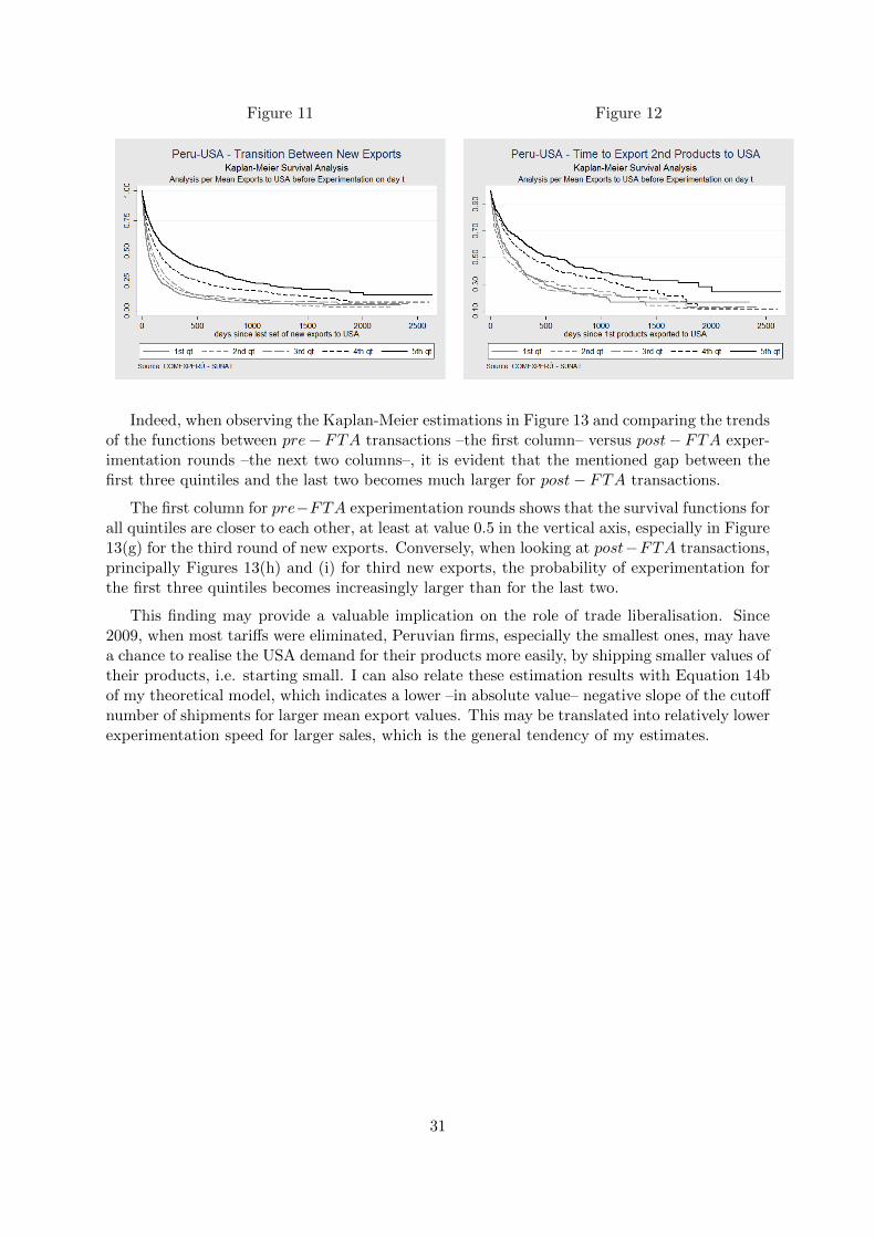
Figure 11 Figure 12

Indeed, when observing the Kaplan-Meier estimations in Figure 13 and comparing the trendsof the functions between pre− FTA transactions –the first column– versus post− FTA exper-imentation rounds –the next two columns–, it is evident that the mentioned gap between thefirst three quintiles and the last two becomes much larger for post− FTA transactions.

The first column for pre−FTA experimentation rounds shows that the survival functions forall quintiles are closer to each other, at least at value 0.5 in the vertical axis, especially in Figure13(g) for the third round of new exports. Conversely, when looking at post−FTA transactions,principally Figures 13(h) and (i) for third new exports, the probability of experimentation forthe first three quintiles becomes increasingly larger than for the last two.

This finding may provide a valuable implication on the role of trade liberalisation. Since2009, when most tariffs were eliminated, Peruvian firms, especially the smallest ones, may havea chance to realise the USA demand for their products more easily, by shipping smaller values oftheir products, i.e. starting small. I can also relate these estimation results with Equation 14bof my theoretical model, which indicates a lower –in absolute value– negative slope of the cutoffnumber of shipments for larger mean export values. This may be translated into relatively lowerexperimentation speed for larger sales, which is the general tendency of my estimates.

31

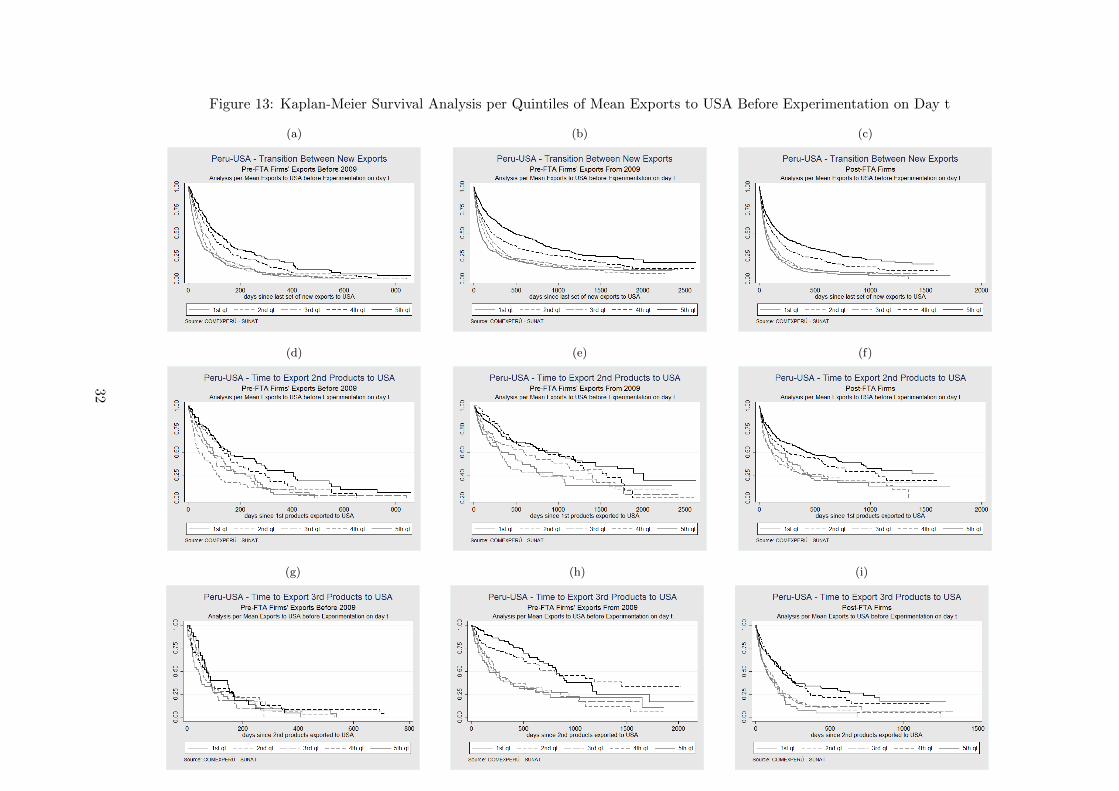
Figure 13: Kaplan-Meier Survival Analysis per Quintiles of Mean Exports to USA Before Experimentation on Day t

(a) (b) (c)

(d) (e) (f)

(g) (h) (i)

32

5.4.2 Mean Exports to All Destinations

Subsequently, I prepared a similar exercise, but working with the mean value of shipmentsby firm i to everywhere, including USA. I reckon this may provide valuable information onexperimentation speed by Peruvian firms, especially for the introduction of their first newproduct to that market.

Similarly, I constructed quintile values for the mean shipments to any destination by firm i,obtaining the following numbers:

• First quintile: mean export value of up to US $ 308.23. This group includes experimen-tation rounds in USA with no previous exports anywhere (zero mean export value).

• Second quintile: above US $ 308.23 and up to US $ 2,148.74.

• Third quintile: above US $ 2,148.74 and up to US $ 6,954.26.

• Fourth quintile: above US $ 6,954.26 and up to US $ 22,452.89.

• Fifth quintile: above US $ 22,452.89.

This analysis gives as interesting results as the former. Figures 14 and 15 show the overallresults for all experimentation rounds and the first new exports, respectively. I am particularlyinterested in the outcome from Figure 15. On the one hand, it is evident that the introductionof a first product to USA preceded by tiny or no shipments to any other destination –the solidgrey line– takes place in a much shorter time span since the firm’s foundation than the firstexperimentations from the other quintiles. This is a sign of the existence of Peruvian firmsexclusively focused on the USA market. Indeed, most debuts in USA from the first quintilecorrespond to firms without any export experience elsewhere.

On the other hand, after the first quintile, the group with the largest experimentation speedis the fifth quintile –the solid black line–, embracing firms with the largest mean export values.This last pattern can be more clearly observed when distinguishing between pre − FTA andpost− FTA transactions.

Figure 14 Figure 15

That analysis, performed in Figure 16, effectively confirms in the second row that the ex-perimentation speed, measured in days since firm i was established, is largest for firms withalmost exclusive focus on the USA market. That speed gap between the first quintile and therest gets exacerbated for first exports by post− FTA firms, as Figure 16(f) shows.

33

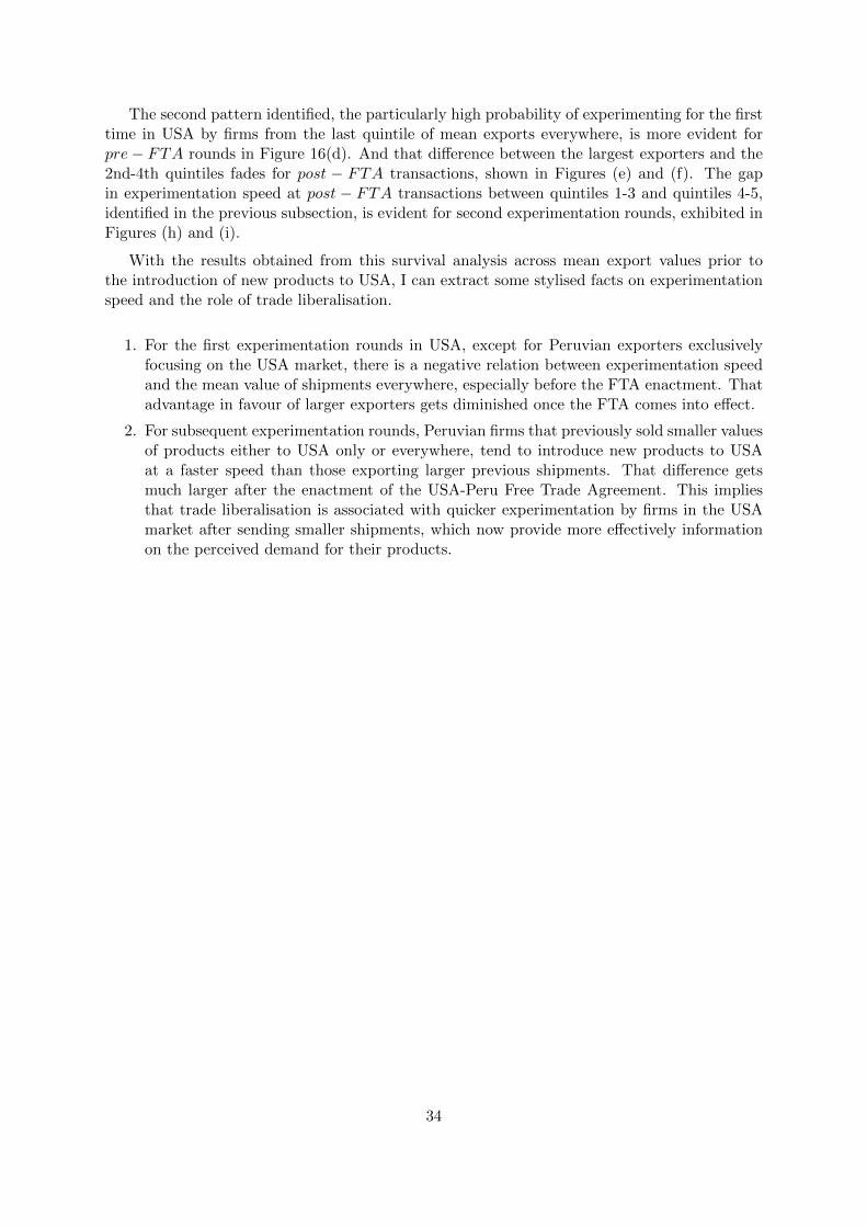
The second pattern identified, the particularly high probability of experimenting for the firsttime in USA by firms from the last quintile of mean exports everywhere, is more evident forpre− FTA rounds in Figure 16(d). And that difference between the largest exporters and the2nd-4th quintiles fades for post − FTA transactions, shown in Figures (e) and (f). The gapin experimentation speed at post − FTA transactions between quintiles 1-3 and quintiles 4-5,identified in the previous subsection, is evident for second experimentation rounds, exhibited inFigures (h) and (i).

With the results obtained from this survival analysis across mean export values prior tothe introduction of new products to USA, I can extract some stylised facts on experimentationspeed and the role of trade liberalisation.

1. For the first experimentation rounds in USA, except for Peruvian exporters exclusivelyfocusing on the USA market, there is a negative relation between experimentation speedand the mean value of shipments everywhere, especially before the FTA enactment. Thatadvantage in favour of larger exporters gets diminished once the FTA comes into effect.

2. For subsequent experimentation rounds, Peruvian firms that previously sold smaller valuesof products either to USA only or everywhere, tend to introduce new products to USAat a faster speed than those exporting larger previous shipments. That difference getsmuch larger after the enactment of the USA-Peru Free Trade Agreement. This impliesthat trade liberalisation is associated with quicker experimentation by firms in the USAmarket after sending smaller shipments, which now provide more effectively informationon the perceived demand for their products.

34

Figure 16: Kaplan-Meier Survival Analysis per Quintiles of Mean Exports to All Destinations Before Experimentation on Day t

(a) (b) (c)

(d) (e) (f)

(g) (h) (i)

35

5.5 Analysis Across Tariff Rates and Preference Regimes

In this next stage of the survival analysis, I am interested in knowing the number of days takenby firms to experiment in the USA market, depending on the mean pre-FTA tariff rate leviedby that country and whether these products enjoyed a USA trade preference regime prior tothe enactment of the Free Trade Agreement. The trade preferences regimes addressed are theAndean Trade Preference and Drug Eradication Act (ATPDEA) and the zero tariff rates underthe WTO Most Favoured Nation (MFN) regime.

5.5.1 Analysis Across Weighted Average Tariffs

As we know, since 2009 the vast majority of products were automatically liberalised (zero tariff).Hence, for the tariff-based analysis to be done, I decided to calculate for each experimentationround a pre-FTA weighted average tariff rate, in which the weight is the US $ export value ofeach product.

I constructed two types of weighted average tariffs: 1) one for all the products sold by firmi on day t; and 2) another one for only the new products introduced by firm i on day t. In thispaper, I present the results from the second type, as my main focus is on the new exports.

For the effects of the calculation of the Kaplan-Meier survival estimator, I obtained thequintiles of the weighted average tariffs, which are as follows:

• First quintile: up to 0.279%, mostly accounting for new products with zero MFN tariff.

• Second quintile: above 0.279% and up to 3.07%.

• Third quintile: above 3.07% and up to 7.34%.

• Fourth quintile: above 7.34% and up to 14.9%.

• Fifth quintile: above 14.9%.

Similar to the mean export analysis, all graphs provided show five step lines, each represent-ing one quintile.

Figure 17 displays the outcome from this exercise, including all experimentation rounds,regardless of the order and the firm. It is clear from this figure that it usually takes a shortertime spell for firms to experiment in USA with products which pre-FTA weighted average tariffbelongs to the 4th –the dashed black line– and, especially, the 5th quintile –the solid black line–.In numbers, firms are faster to export new goods with an over 7.34% pre-FTA weighted averagerate. On the contrary, firms take much longer to export new products from the 1st quintile,namely, those with zero MFN tariffs. It must be pointed out, nevertheless, that products fromsuch 1st quintile are more quickly exported by firms in much further rounds, even quicker thanproducts from the top quintiles.

This first finding may imply an opposite result compared to the basics of my sequentialexporting theory, which stated that, between two types of products, the firm would experimentwith the one with the lowest trade cost. However, recall that some of the tariff lines exportedbefore the 2009 FTA, be from either the lowest or highest quintiles, enjoyed a zero tariff underthe ATPDEA regime by USA.

36

Figure 17

Additionally, the export behaviour by firms may vary between pre−FTA and post−FTAfirms. Figure 18 compiles that analysis, across pre-FTA tariff quintiles and distinguishingbetween transactions done before and from 2009.

The first row confirms the findings from the previous figure, in that new products belongingto the 4th and 5th pre-FTA tariff rate quintiles tend to wait less to be introduced than productswith lower trade costs. This tendency for pre − FTA firms, however, is more evident for thepost-FTA new exports (Figure 18(b)), in which nearly all tariffs become zero. Clearly, in thatcase new exports of the furthest quintiles are more dynamic than exports of the 2nd –the dashedgrey line– and 3rd quintiles –the dashed and dotted grey line–, and even more dynamic thanthose of the 1st quintile –the solid grey line representing the zero MFN tariff group–. In Figure18(b), the probability of introducing new products to USA becomes 50% at 123 days since thefirm’s last experimentation round for transactions from the 4th quintile by pre − FTA firmsdone since 2009; while for the 5th quintile, that probability is achieved 22 days later. Fairlylonger spells are taken by new exports of products with lower weighted average tariffs.

When looking at the first and second experimentation rounds, the finding described earlieralso holds. Products with the highest pre-FTA tariffs tend to take less to be exported after theFTA by more experienced firms. Particularly, the second experimentation round of productsfrom the top quintile (Figure 18(h)) are by far more dynamic than the rest. Such tendency wasalso found for the second rounds by post − FTA firms (Figure 18(i)). It must be pointed outthough that for further rounds, the duration difference between low and high tariff productsdiminishes considerably. Hence, it can be argued that there is an experimentation peak for themost costly products at the second round of post-FTA transactions, followed by more experi-mentation with products with lower pre-FTA tariffs in further rounds. Relating these resultswith Equation 14a of my theoretical model, I highlight that for post − FTA experimentationrounds by both types of firms, the gap between the top two tariff quintiles and the rest becomeslarger, meaning that trade liberalisation’s experimentation accelerating role is more relevant forproducts with highest pre− FTA tariffs.

37

Figure 18: Kaplan-Meier Survival Analysis per Weighted Average Pre-FTA Tariffs (new exports)

(a) (b) (c)

(d) (e) (f)

(g) (h) (i)

38

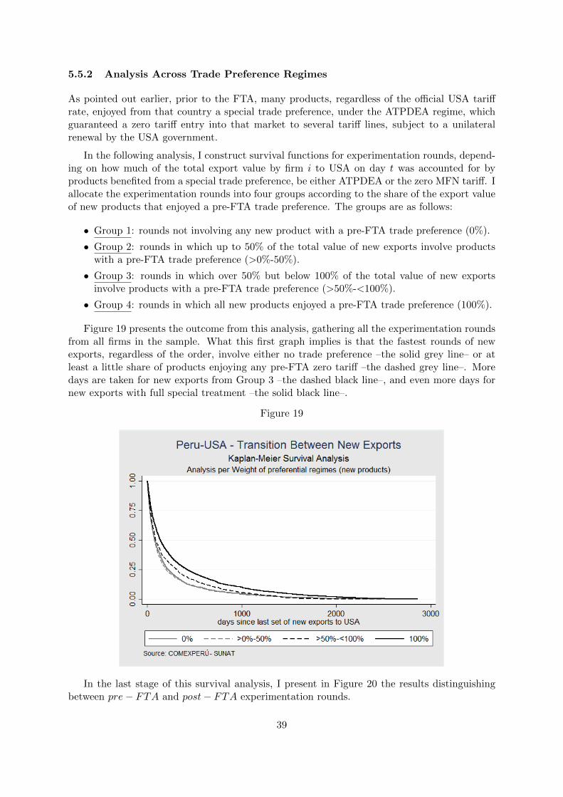
5.5.2 Analysis Across Trade Preference Regimes

As pointed out earlier, prior to the FTA, many products, regardless of the official USA tariffrate, enjoyed from that country a special trade preference, under the ATPDEA regime, whichguaranteed a zero tariff entry into that market to several tariff lines, subject to a unilateralrenewal by the USA government.

In the following analysis, I construct survival functions for experimentation rounds, depend-ing on how much of the total export value by firm i to USA on day t was accounted for byproducts benefited from a special trade preference, be either ATPDEA or the zero MFN tariff. Iallocate the experimentation rounds into four groups according to the share of the export valueof new products that enjoyed a pre-FTA trade preference. The groups are as follows:

• Group 1: rounds not involving any new product with a pre-FTA trade preference (0%).

• Group 2: rounds in which up to 50% of the total value of new exports involve productswith a pre-FTA trade preference (>0%-50%).

• Group 3: rounds in which over 50% but below 100% of the total value of new exportsinvolve products with a pre-FTA trade preference (>50%-<100%).

• Group 4: rounds in which all new products enjoyed a pre-FTA trade preference (100%).

Figure 19 presents the outcome from this analysis, gathering all the experimentation roundsfrom all firms in the sample. What this first graph implies is that the fastest rounds of newexports, regardless of the order, involve either no trade preference –the solid grey line– or atleast a little share of products enjoying any pre-FTA zero tariff –the dashed grey line–. Moredays are taken for new exports from Group 3 –the dashed black line–, and even more days fornew exports with full special treatment –the solid black line–.

Figure 19

In the last stage of this survival analysis, I present in Figure 20 the results distinguishingbetween pre− FTA and post− FTA experimentation rounds.

39

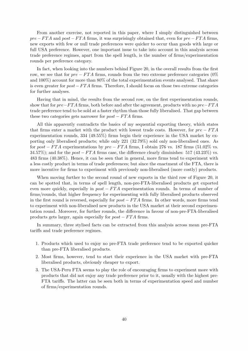
From another exercise, not reported in this paper, where I simply distinguished betweenpre−FTA and post−FTA firms, it was surprisingly obtained that, even for pre−FTA firms,new exports with few or null trade preferences were quicker to occur than goods with large orfull USA preference. However, one important issue to take into account in this analysis acrosstrade preference regimes, apart from the spell length, is the number of firms/experimentationrounds per preference category.

In fact, when looking into the numbers behind Figure 20, in the overall results from the firstrow, we see that for pre− FTA firms, rounds from the two extreme preference categories (0%and 100%) account for more than 80% of the total experimentation events analysed. That shareis even greater for post−FTA firms. Therefore, I should focus on those two extreme categoriesfor further analyses.

Having that in mind, the results from the second row, on the first experimentation rounds,show that for pre−FTA firms, both before and after the agreement, products with no pre−FTAtrade preference tend to be sold at a faster rhythm than those fully liberalised. That gap betweenthese two categories gets narrower for post− FTA firms.

All this apparently contradicts the basics of my sequential exporting theory, which statesthat firms enter a market with the product with lowest trade costs. However, for pre − FTAexperimentation rounds, 334 (49.55%) firms begin their experience in the USA market by ex-porting only liberalised products; while only 221 (32.79%) sold only non-liberalised ones. Asfor post − FTA experimentations by pre− FTA firms, I obtain 276 vs. 187 firms (51.02% vs.34.57%); and for the post−FTA firms case, the difference clearly diminishes: 517 (43.23%) vs.483 firms (40.38%). Hence, it can be seen that in general, more firms tend to experiment witha less costly product in terms of trade preferences; but since the enactment of the FTA, there ismore incentive for firms to experiment with previously non-liberalised (more costly) products.

When moving further to the second round of new exports in the third row of Figure 20, itcan be spotted that, in terms of spell length, non-pre-FTA-liberalised products get exportedeven more quickly, especially in post − FTA experimentation rounds. In terms of number offirms/rounds, that higher frequency for experimenting with fully liberalised products observedin the first round is reversed, especially for post− FTA firms. In other words, more firms tendto experiment with non-liberalised new products in the USA market at their second experimen-tation round. Moreover, for further rounds, the difference in favour of non-pre-FTA-liberalisedproducts gets larger, again especially for post− FTA firms.

In summary, three stylised facts can be extracted from this analysis across mean pre-FTAtariffs and trade preference regimes.

1. Products which used to enjoy no pre-FTA trade preference tend to be exported quickerthan pre-FTA liberalised products.

2. Most firms, however, tend to start their experience in the USA market with pre-FTAliberalised products, obviously cheaper to export.

3. The USA-Peru FTA seems to play the role of encouraging firms to experiment more withproducts that did not enjoy any trade preference prior to it, usually with the highest pre-FTA tariffs. The latter can be seen both in terms of experimentation speed and numberof firms/experimentation rounds.

40

Figure 20: Kaplan-Meier Survival Analysis per Weight of USA Pre-FTA Preferential Regimes (new exports)

(a) (b) (c)

(d) (e) (f)

(g) (h) (i)

41

6 Econometric Approach

After that first attempt to test some features of my theoretical prediction by a Kaplan-Meiersurvival analysis, in this section I present the main results from the econometric models, aimingto provide an alternative approach to test some of the main predictions from the theory.

6.1 Number of Shipments

I start by running an Ordinary Least Square (OLS) identification strategy, in which each ob-servation represents the event of the introduction of one or many products by firm i into theUSA market, i.e. experimentation round. As in the descriptive and survival analyses, theseestimations consider Peruvian firms starting to export USA between 2006 and 2013. Since mypurpose is to assess the influence of trade liberalisation and the value of exports on the numberof shipments prior to an experimentation round, I propose the following basic specification:

num shipments USAi = α0 + α1postftai + α2mean export USAi+

α3postfta ∗ export USAi + α4new wmean tariffi+

α5postfta ∗ tariffi + µijt

(16)

This first approach takes every experimentation round independently, regardless of the firm,because a panel fixed effects model at the firm level, shown afterwards, omits some relevantvariables I am interested in.

The dependent variable is the log of the number of shipments to USA by a Peruvian firmbefore experimentation round i, from experimentation round i − 1 inclusively. That variableis regressed on postfta, a dummy variable taking value 1 if the Peruvian firm making ex-perimentation round i was founded between 2009 and 2013, when the USA-Peru Free TradeAgreement came into force. mean export USA stands for the log of the firm’s mean exportvalue of shipments to USA from experimentation round i − 1 to the last shipment before ex-perimentation round i. These first two variables are interacted to see if there is a combinedeffect. Aiming to find a more specific effect of trade liberalisation at the product level, I includenew wmean tariff , the log of one plus the average pre-FTA tariffs levied on the new productsexported in experimentation round i, weighted by the export value per product. Thus, tariffslevied on products accounting for the largest shares of the full experimentation shipment aregiven more weight. That variable is also interacted with the postfta dummy.

Further additions and modifications are made to that basic specification. Firstly, I incorpo-rate the pre postfta dummy, taking value 1 if experimentation round i was done by a pre−FTAPeruvian firm after the enactment of the USA-Peru FTA. By adding this dummy, and keepingthe postfta variable, pre − FTA experimentation rounds by pre − FTA firms become nowthe base category. pre postfta is afterwards interacted with the export and tariff variables.Secondly, I replace the tariff regressor by new wpref , standing for the proportion, weighted byexport values, of new products exported in experimentation round i eligible for a pre − FTAtrade preferential regime, either ATPDEA or zero-MFN tariffs. I interact this last variable withthe postfta and pre postfta dummies.

This first approach and the subsequent ones all include year and sector fixed effects, as wellas other controllers used in the survival analysis, such as a dummy for many products per round,another one for the elsewhere experience, and others for first and second experimentation rounds

42

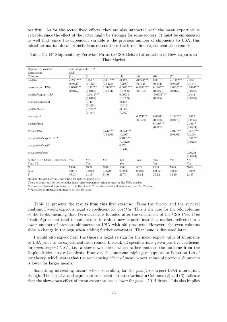
per firm. As for the sector fixed effects, they are also interacted with the mean export valuevariable, since the effect of the latter might be stronger for some sectors. It must be emphasisedas well that, since the dependent variable is the previous number of shipments to USA, thisinitial estimation does not include as observations the firms’ first experimentation rounds.

Table 11: N◦ Shipments by Peruvian Firms to USA Before Introduction of New Exports toThat Market

Dependent Variable num shipments USAEstimation OLSColumn (1) (2) (3) (4) (5) (6) (7) (8)

postfta -0.271*** 0.251* -0.116*** -0.123 -0.273*** 0.0616 -0.112*** -0.266(0.0325) (0.132) (0.0428) (0.196) (0.0325) (0.132) (0.0428) (0.194)

mean export USA 0.0961*** 0.133*** 0.0923*** 0.0632*** 0.0950*** 0.128*** 0.0910*** 0.0584***(0.0152) (0.0166) (0.0153) (0.0208) (0.0153) (0.0166) (0.0153) (0.0207)

postfta*export USA -0.0644*** 0.00915 -0.0587*** 0.0144(0.0159) (0.0209) (0.0159) (0.0209)

new wmean tariff 0.140 -0.158(0.425) (0.614)

postfta*tariff -0.975** -0.685(0.484) (0.660)

new wpref 0.174*** 0.0981* 0.182*** 0.0912(0.0480) (0.0584) (0.0479) (0.0836)

postfta*pref 0.190*** 0.196**(0.0719) (0.0924)

pre postfta 0.232*** -0.631*** 0.241*** -0.570***(0.0460) (0.203) (0.0462) (0.200)

pre postfta*export USA 0.106*** 0.105***(0.0222) (0.0221)

pre postfta*tariff 0.470(0.734)

pre postfta*pref 0.00258(0.0994)

Sector FE / Other Regressors Yes Yes Yes Yes Yes Yes Yes YesYear FE Yes Yes Yes Yes

N 5036 5009 5036 5009 5028 5028 5028 5028r2 o 0.0573 0.0919 0.0620 0.0966 0.0600 0.0945 0.0650 0.0992F 36.63 24.19 34.58 21.70 33.62 25.12 32.10 22.55

Robust standard errors controlling for heteroskedasticity.These estimations do not consider firms’ first experimentation rounds in the USA market.*Denotes statistical significance at the 10% level; **Denotes statistical significance at the 5% level;***Denotes statistical significance at the 1% level.

Table 11 presents the results from this first exercise. From the theory and the survivalanalysis, I would expect a negative coefficient for postfta. This is the case for the odd columnsof the table, meaning that Peruvian firms founded after the enactment of the USA-Peru FreeTrade Agreement tend to wait less to introduce new exports into that market, reflected in alower number of previous shipments to USA with old products. However, the even columnsshow a change in the sign when adding further covariates. That issue is discussed later.

I would also expect from the theory a negative sign for the mean export value of shipmentsto USA prior to an experimentation round. Instead, all specifications give a positive coefficientfor mean export USA, i.e. a slow-down effect, which rather matches the outcome from theKaplan-Meier survival analysis. However, this outcome might give support to Equation 14b ofmy theory, which states that the accelerating effect of mean export values of previous shipmentsis lower for larger means.

Something interesting occurs when controlling for the postfta ∗ export USA interaction,though. The negative and significant coefficient of that covariate in Columns (2) and (6) indicatethat the slow-down effect of mean export values is lower for post−FTA firms. This also implies

43

an increasingly accelerating postfta effect for higher mean exports. Focusing on Column (2), letme explore the net effects. Assuming a zero pre−FTA tariff, the net effect of a 1% increase inthe mean export value on the number of shipments is 0.133% for a pre−FTA firm, and 0.0683%for a post − FTA firm. More interestingly, taking the median value of the mean export USAvariable for post − FTA firms (US $ 4,077.33), the net effect of the postfta dummy on thenumber of shipments to USA prior to an experimentation round is approximately -25%, beingonly US $ 49.28 the mean export value at which the postfta effect cancels out. The patterndescribed remains consistent across most specifications and methods I present in this document,and may be interpreted as follows: the effect of being a post − FTA firm on experimentationspeed is mostly positive, expressed in fewer shipments to USA prior to a new experimentationround compared to pre− FTA firms, turning negative only for rounds preceded by very smallconsignments of products previously introduced.

As for the weighted mean pre − FTA tariff, my theory’s proposition make me expect apositive coefficient; but Columns (2) and (4) do not give significant numbers. These two columnsalso include the interaction with postfta, which obtains a negative and significant value inColumn (2). Again, this sign is consistent across further estimations shown afterwards, and isreasonable to expect, as after the FTA enactment most tariffs are eliminated, facilitating thedecision to experiment in USA, especially for products with higher pre−FTA tariffs. Moreover,going back to the change in the sign of postfta from Column (1) to (2), for instance, I can arguethat the effect of being a post − FTA firm on experimentation speed is an accelerating effectfor most products, except for those with zero or a minimum pre− FTA tariff.

But what is the effect on number of shipments for pre − FTA firms experimenting afterthe FTA enactment? To address this concern, in Columns (3) and (4) I add the pre postftadummy. Column (3) shows a positive and significant coefficient for that dummy, meaning thatexperimentation rounds after the FTA by pre − FTA firms are preceded by more shipmentsthan rounds before the FTA by those firms. This outcome may reflect cases where, for instance,firms founded in 2006 try to experiment in 2013, long after the FTA enactment. Hence, suchexperimentation round may be preceded by more shipments than an equivalent event by anotherpre− FTA firm before the agreement came into effect.

When adding the interactions in Column (4), the sign for pre postfta becomes insteadnegative, with the previous positive effect being transferred to the interaction with the meanexport values. Again, let me go through the net effects, assuming zero tariffs. The positiveeffect of a 1% increase of mean export USA on the number of shipments to USA is 0.0632%for both pre−FTA experimentation rounds and those done by post−FTA firms; whereas it is0.2161% for post− FTA rounds by pre− FTA firms. As for effect of the pre postfta dummy,taking the 10th percentile of mean export USA for post − FTA rounds by pre − FTA firms(US $ 215.29), that effect is approximately -6%, and turns into positive when the mean exportvalue exceeds US$ 384.84, which lies far below the median and average of that variable.

The described outcome can be interpreted as follows: the effect of being a pre−FTA firm ex-perimenting after the FTA enactment is mostly a slow-down effect, compared to experimentingbefore the agreement; but it is an accelerating one for rounds preceded by very small shipmentsof products already introduced, i.e. after starting small with those products. This result isslightly in line with the outcome from Equation 14a of my theoretical model, in that the ef-fect of a tariff change on experimentation speed is lower the larger the mean value of previousshipments is. No significant effect is found for the interaction of pre postfta with tariffs.

Columns (5)-(8) replicate the analysis, but replacing the tariff variable by the new wprefregressor, accounting for the pre−FTA unilateral trade preference share of the new exports in

44

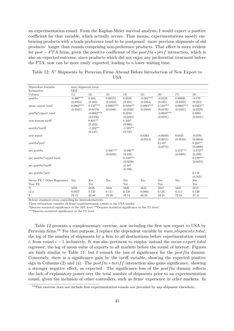
an experimentation round. From the Kaplan-Meier survival analysis, I would expect a positivecoefficient for that variable, which actually occurs. That means, experimentations mostly em-bracing products with a trade preference tend to be postponed –more previous shipments of oldproducts– longer than rounds comprising non-preference products. That effect is more evidentfor post − FTA firms, given the positive coefficient of the postfta ∗ pref interaction, which isalso an expected outcome, since products which did not enjoy any preferential treatment beforethe FTA, now can be more easily exported, leading to a lower waiting time.

Table 12: N◦ Shipments by Peruvian Firms Abroad Before Introduction of New Export toUSA

Dependent Variable num shipments totalEstimation OLSColumn (1) (2) (3) (4) (5) (6) (7) (8)

postfta -0.300*** 0.164 0.00574 0.0558 -0.301*** -0.0123 0.00800 -0.170(0.0354) (0.165) (0.0458) (0.231) (0.0354) (0.165) (0.0459) (0.224)

mean export total 0.0962*** 0.137*** 0.0904*** 0.0488** 0.0964*** 0.134*** 0.0904*** 0.0462**(0.0167) (0.0179) (0.0166) (0.0230) (0.0168) (0.0179) (0.0167) (0.0229)

postfta*export total -0.0682*** 0.0240 -0.0645*** 0.0265(0.0190) (0.0242) (0.0191) (0.0241)

new wmean tariff 0.891** 1.240*(0.453) (0.666)

postfta*tariff -1.224** -1.591**(0.547) (0.735)

new wpref 0.0264 -0.00565 0.0455 -0.0791(0.0514) (0.0615) (0.0510) (0.0883)

postfta*pref 0.148* 0.224**(0.0774) (0.0990)

pre postfta 0.466*** -0.496** 0.472*** -0.573**(0.0494) (0.239) (0.0495) (0.230)

pre postfta*export total 0.140*** 0.139***(0.0256) (0.0255)

pre postfta*tariff -0.487(0.796)

pre postfta*pref 0.116(0.105)

Sector FE / Other Regressors Yes Yes Yes Yes Yes Yes Yes YesYear FE Yes Yes Yes Yes

N 5859 5826 5859 5826 5847 5847 5847 5847r2 o 0.0977 0.135 0.111 0.139 0.0981 0.135 0.111 0.139F 78.12 42.88 79.90 37.12 69.55 43.21 72.18 37.41

Robust standard errors controlling for heteroskedasticity.These estimations consider all firms’ experimentation rounds in the USA market.*Denotes statistical significance at the 10% level; **Denotes statistical significance at the 5% level;***Denotes statistical significance at the 1% level.

Table 12 presents a complementary exercise, now including the first new export to USA byPeruvian firms.12 For that purpose, I replace the dependent variable by num shipments total,the log of the number of shipments by a firm to all destinations before experimentation roundi, from round i − 1 inclusively. It was also pertinent to employ instead the mean export totalregressor, the log of mean value of exports to all markets before the round of interest. Figuresare fairly similar to Table 11; but I remark the loss of significance for the postfta dummy.Conversely, there is a significance gain by the tariff variable, showing the expected positivesign in Columns (2) and (4). The postfta ∗ tariff interaction also gains significance, showinga stronger negative effect, as expected. The significance loss of the postfta dummy reflectsthe lack of explanatory power over the total number of shipments prior to an experimentationround, given the inclusion of other controllers, such as firms’ experience in other markets. In

12This exercise does not include first experimentation rounds not preceded by any shipment elsewhere.

45

fact, the elsewhere dummy, not reported in this table, always shows highly significant positivecoefficients, implying that focusing on other markets may prompt firms to postpone the decisionto export a new product to USA, especially for the first experimentation.

Appendix B shows replications of this OLS approach, considering either only the first exper-imentation round per firm, using the shipments to all destinations, or only the second round.For the latter, I run regressions for both types of dependent variables. On first experimentationrounds, it is striking that postfta is positive in all specifications, and significant when addingthe pre postfta dummy. That may be explained by the aforementioned time difference betweenan experimentation round made in 2013 by a post−FTA firm founded early in 2009, comparedto a round produced in 2008 by a pre−FTA firm founded in 2006. Additionally, the new wprefvariable on the pre−FTA unilateral trade preference by USA, always gives negative and signif-icant coefficients, which makes sense, since firms that start their export activity in USA before2009, tend to do it with fully liberalised products, as discussed in the survival analysis.

When it comes to analysing the second experimentation rounds, taking num shipments USAas dependent variable, it is remarkable that postfta keeps its negative and significant value evenwhen controlling for post − FTA rounds by pre − FTA firms. This may imply that trade lib-eralisation exerts a trigger to grow in the USA market at the early extensive margin for firmsfounded after the FTA enactment. That effect does not seem to come from the tariff elimi-nation, given the insignificant coefficients for the tariff variables. I did the same exercise fornum shipments total, and no major differences from the main outcomes in Table 12 are found.

Appendix C presents a panel data model with fixed effects at the firm level. This strategydoes not allow to distinguish the effect of being a post−FTA firm per se, since that dummy getsomitted; but we can interact it. The mean exports to USA or all destinations keeps its positiveand significant effect; but the interaction with postfta loses significance in most specifications.Tariff variables are not significant, but they show consistency in the signs across columns. Infact, higher tariffs are associated with a longer delay in experimentation; but the interactionfor post − FTA firms is linked to an acceleration. All this gives support to the main findingspresented earlier. Equal consistency is shown by the trade preference variables. Positive values,although insignificant, for new wpref ; but negative and significant coefficient for the interactionwith postfta, implying an experimentation acceleration for post−FTA firms exporting productsnot subject to any pre−FTA preference. No relevant changes for the pre postfta combinations,confirming the tendency for pre−FTA firms to experiment quicker since the enactment of theFTA after starting small in the USA market. Although not reported, the many dummy, onexperimentation rounds with more than one product, is consistently negative and significant,providing an approach of the relevance of firms’ size.

Overall, the results described show an apparent incompatibility between my theory’s pre-diction and the empirical finding on the role of export values. That outcome leads me to thinkabout the limitations of my approach. The observed delay in the introduction of a new productassociated with larger shipments of previous goods might be due to a firm-specific decision tosufficiently enjoy the profitability in market d generated by exporting product A, which is notcontemplated in my theory. Additionally, my empirical approach accounts in a preliminary wayfor firms’ experience in other markets, by including a dummy taking value 1 if, in the monthprior to the experimentation round, the firm has exported elsewhere. Clearly, further attemptscan be made to account for that experience.

I am aware as well that the number of shipments of a product is not a perfect indicator ofexperimentation speed, since few shipments may occur within a long period of time, and theshipment frequency may also depend on the industry the product belongs to. This is to some

46

extent tackled here by controlling for sector fixed effects of the new product introduced; but itwould also be relevant to control for the industry of the old products; although most old andnew products belong to the same industry.

6.2 Duration Model

Aiming to offer a closer complement to the earlier Kaplan-Meier survival analysis, I run a CoxProportional Hazard Model, a continuous-time duration model proposed by Cox (1972), whichestimates the hazard function for every individual from a sample, in the following general shape:

h(t) = h0(t)exp(β1x1 + . . .+ βkxk) (17)

where h(t) is the hazard at time t for an observation; h0(t) is the baseline hazard, not estimatedin this model; and the rest of the right hand side stands for the covariates considered. The CoxModel calculates the probability of a failure to occur to an individual at time t. I opted for acontinuous-time model like Cox given the nature of the time spells constructed.

As in my earlier approach, observations are at the experimentation round level; and the timespell considered is the number of days prior to the event of a firm’s experimentation round isince the day of firm’s round i−1 inclusively. Hence, the event of a Peruvian firm introducing anew export to the USA market is the “failure” in this analysis, and I measure the probability ofthat “failure” occurring at day t since the firm’s previous “failure”, or since the firm’s foundationdate, in case of its first experimentation round.

It is important to point out that, as many of my covariates are at the product level, this ex-ercise does not include censored observations. And, more importantly, given the likely existenceof risk heterogeneity at the firm level, I run a Cox model with shared frailty at such level.

Tables 13 and 14 report the hazard ratios (exp(βk)) using the same regressors from theOLS analysis. Hazard ratios above unity mean that the covariate increases the probability ofintroducing new exports to USA; whereas ratios below unity represent a fall in that likelihood.

47

Table 13: Peruvian Firms’ Probability of Introducing New Exports to USA (Hazard Ratios)Excluding First Experimentation Rounds

Time Spell Days After Firm i’s Last Experimentation Round in USAEstimation Cox Proportional Hazard Model - Shared Frailty at Firm LevelColumn (1) (2) (3) (4) (5) (6) (7) (8)

postfta 1.629*** 1.796*** 0.985 0.293*** 1.626*** 2.199*** 0.982 0.345***(0.0857) (0.329) (0.0608) (0.0742) (0.0853) (0.401) (0.0603) (0.0864)

mean export USA 0.846*** 0.861*** 0.849*** 0.857*** 0.846*** 0.863*** 0.849*** 0.860***(0.0146) (0.0160) (0.0147) (0.0217) (0.0146) (0.0161) (0.0147) (0.0217)

postfta*export USA 1.022 1.026 1.019 1.021(0.0208) (0.0273) (0.0208) (0.0271)

new wmean tariff 1.908** 0.649 1.784* 1.023(0.582) (0.263) (0.546) (0.671)

postfta*tariff 4.327*** 2.759(2.272) (2.037)

new wpref 0.901** 0.967 0.886** 1.032(0.0431) (0.0559) (0.0425) (0.0919)

postfta*pref 0.851** 0.795**(0.0678) (0.0833)

pre postfta 0.477*** 0.171*** 0.474*** 0.162***(0.0245) (0.0407) (0.0242) (0.0380)

pre postfta*export USA 1.003 1.003(0.0249) (0.0248)

pre postfta*tariff 0.475(0.353)

pre postfta*pref 0.911(0.0922)

FE 2009 0.283*** 2.023*** 0.275*** 2.009***(0.0372) (0.134) (0.0356) (0.133)

FE 2010 0.219*** 1.542*** 0.213*** 1.548***(0.0290) (0.0910) (0.0279) (0.0913)

FE 2011 0.169*** 1.187*** 0.165*** 1.192***(0.0225) (0.0637) (0.0216) (0.0638)

Sector FE / Other Regressors Yes Yes Yes Yes Yes Yes Yes YesYear FE Yes Yes Yes Yes

N 5025 5025 5025 5025 5044 5044 5044 5044chi2 340.4 764.1 539.3 766.9 341.2 772.4 545.9 774.4theta 0.350 0.282 0.339 0.282 0.349 0.283 0.338 0.283

Robust standard errors adjusted for clusters in firms.*Denotes statistical significance at the 10% level; **Denotes statistical significance at the 5% level;***Denotes statistical significance at the 1% level.

Table 13 shows the results excluding the first experimentation round per firm, in order tosee the effect of the mean exports to USA only. To understand the interpretation of hazardratios, let me focus on Column (1). Being a post − FTA firm increases in 62.9% a Peruvianfirm’s probability of introducing a new set of products to the USA market at time t, comparedto a pre−FTA firm. For covariates in natural logs, the interpretation is different: an e-fold risein a firm’s mean export value to USA (multiplied by e = 2.718) since its last experimentationround reduces the new experimentation likelihood in 15% approximately; and an e-fold rise inthe pre− FTA tariff on products raises the experimentation probability in about 91%.

As in the OLS approach, the role of the postfta dummy turns into the opposite whenincluding the pre postfta regressors; and the mean export value keeps its hazard-reducingfunction across all specifications. Regarding the tariff variable, when including its interactionwith postfta, it loses significance and even gets its role reversed; while the interaction turnsout highly significant, with a clear role of increasing the experimentation probability in Column(2), meaning that post − FTA firms tend to experiment faster in the USA market with goodspreviously charged with high tariffs. The figures for the new wpref variables are in line withthe outcome from the previous analyses: firms tend to experiment earlier in the USA market

48

with products with no pre−FTA unilateral trade preference by USA, especially firms foundedafter the FTA enactment.

An important difference with respect to the OLS estimations occur with the pre postftavariables accounting for post− FTA experimentation rounds by pre− FTA firms. The signif-icant coefficients below unity for pre postfta in all specifications imply that this category ofexperimentation tends to take more days to occur than experimentation rounds made before theFTA enactment, which makes sense given the time comparisons mentioned earlier between preand post−FTA experimentation rounds by pre−FTA firms. However, interactions, especiallythat with the mean export value, are all insignificant. This differs from the previous analysis,where pre postfta experimentation rounds preceded by small shipments tended to occur faster.

Apparently, the inclusion of the pre postfta covariates discards any accelerating effect oftrade liberalisation. Nevertheless, Columns (4) and (8) control for year fixed effects, whichhazard ratios are worthy to refer to. While 2007 and 2008 dummies have a slow-down effect onexperimentation, that effect dramatically reverses into acceleration for 2009, the year of the FTAenactment. In fact, the experimentation probability increases by more than 100% in that yearwith respect to 2006, the base year. In other words, a Peruvian firm in 2009 is over 100% morelikely to experiment in USA than a firm in 2006, t days after their last experimentation rounds.That effect lowers to around 54% for 2010 and 19% for 2011. Hence, these results confirmthat there is an effect from trade liberalisation in favour of faster export experimentation byPeruvian firms in the USA market.13

13The estimations from the Cox Proportional Hazard approach control for year fixed effects from 2007 to 2013;but only coefficients for 2009-2011 dummies are reported in this paper.

49

Table 14: Peruvian Firms’ Probability of Introducing New Exports to USA (Hazard Ratios)Including First Experimentation Rounds

Time Spell Days After Firm i’s Last Experimentation Round in USA or Entry into Business (1st Round)Estimation Cox Proportional Hazard Model - Shared Frailty at Firm LevelColumn (1) (2) (3) (4) (5) (6) (7) (8)

postfta 1.710*** 1.576** 1.090 0.211*** 1.524*** 1.808*** 1.141** 0.288***(0.0849) (0.297) (0.0615) (0.0529) (0.0867) (0.373) (0.0736) (0.0780)

mean export total 0.820*** 0.856*** 0.823*** 0.865*** 0.802*** 0.838*** 0.805*** 0.835***(0.0143) (0.0155) (0.0143) (0.0210) (0.0151) (0.0168) (0.0151) (0.0228)

postfta*export total 1.052** 1.035 1.043* 1.047(0.0216) (0.0270) (0.0238) (0.0305)

new wmean tariff 1.396 0.658 1.230 0.628(0.415) (0.249) (0.367) (0.377)

postfta*tariff 5.255*** 5.309**(2.533) (3.575)

new wpref 0.893** 0.964 0.886** 1.045(0.0433) (0.0556) (0.0430) (0.0927)

postfta*pref 0.841** 0.773**(0.0670) (0.0808)

pre postfta 0.501*** 0.157*** 0.641*** 0.166***(0.0238) (0.0371) (0.0325) (0.0417)

pre postfta*export total 0.973 1.004(0.0238) (0.0272)

pre postfta*tariff 0.883(0.601)

pre postfta*pref 0.890(0.0899)

FE 2009 0.225*** 2.577*** 0.276*** 1.986***(0.0263) (0.162) (0.0358) (0.132)

FE 2010 0.159*** 1.810*** 0.218*** 1.556***(0.0189) (0.100) (0.0286) (0.0917)

FE 2011 0.120*** 1.337*** 0.168*** 1.193***(0.0143) (0.0677) (0.0221) (0.0639)

Sector FE / Other Regressors Yes Yes Yes Yes Yes Yes Yes YesYear FE Yes Yes Yes Yes

N 5832 5832 5832 5832 5853 5853 5853 5853chi2 498.6 1808.4 708.7 1786.1 595.2 795.0 673.9 797.3theta 0.473 0.245 0.438 0.263 0.665 0.287 0.642 0.287

Robust standard errors adjusted for clusters in firms.*Denotes statistical significance at the 10% level; **Denotes statistical significance at the 5% level;***Denotes statistical significance at the 1% level.

No major changes to the commented results occur in Table 14 where I add the first experi-mentation rounds to measure the effect of mean export values to all destinations. Perhaps, I mayhighlight that in the first four columns the accelerating role of the postfta variables is stronger,since the interaction with export values recovers its significance, as in the OLS approach; andthe interaction with tariffs provides a more evident effect in favour of experimentation. Thatmeans, postfta firms experiment faster with products with higher pre−FTA tariffs after havingshipped large export values abroad.

Very similar results are obtained for Cox estimations without shared frailty, with standarderrors clustered at the firm level, presented in Appendix D. I also present in Appendix E separateCox estimations for first and second experimentation rounds. Results do not differ from theshared frailty exercise nor the OLS estimations; but I can remark that the aforementionedacceleration effects arising from the year fixed effects after the FTA enactment get dramaticallyinflated for these first two experimentation rounds, especially the first one. The 2009 dummyprovides a 2,000% jump in the probability to send a first shipment to USA; while a 660% and350% probability rise are given by the 2010 and 2011 dummies, respectively.

50

7 Conclusions

This paper investigates the strategy firms undertake to penetrate into one particular destina-tions, by exporting new products sequentially. More precisely, I am interested in how quicklyfirms experiment with a new product in that market, after having done so with other previousproducts there.

For that purpose, I develop a theoretical model where product demands follow a joint bi-variate distribution, imperfectly correlated. By sending shipments of the cheaper product A tomarket d, thereby realising the demand for A, a firm gradually updates its expected demandfor the more costly product B. Thus, that expected demand for B is in function of the numberof shipments of A, as well as the demand correlation of both products, and the mean value ofthose shipments.

As a result, my model predicts that experimentation speed in a sequential exporting strategyis greater (i.e. less shipments of A before introduction of B) with (i) lower trade costs of productB; (ii) larger mean export values of A to market d; and (iii) higher correlation between thedemand for the two products in d. The magnitude of these effects clearly depend on the initialvalues of those variables.

This prediction is empirically tested with a survival analysis, comprising a Kaplan-Meiersurvival estimation and a Cox proportional hazard model, along with an OLS and panel dataapproach, using a very rich dataset of Peruvian exports to the USA market, covering the 2006-2013 period. The data was processed to obtain a set of observations, each representing theevent in which a Peruvian firm introduces a new product to the USA market, known in thispaper as an experimentation round. I give a special emphasis on the role of trade liberalisation,expressed as the tariff elimination by the United States on Peruvian products, under the FreeTrade Agreement signed by both countries in 2009. Thus, this paper is one of the first attemptsto measure the effects of this FTA on Peruvian exporters’ performance in the USA market.

Overall, the prediction from my theoretical approach finds empirical support regarding theeffect of trade liberalisation on experimentation speed. This can be observed in several ways.Firstly, post − FTA firms, founded after the FTA came into force, tend to introduce newproducts to USA faster than pre − FTA firms, expressed in either fewer previous shipmentsof other products to that market or fewer days since the introduction of the previous product.Secondly, that process is even quicker when the product used to face a high tariff prior to theFTA enactment and/or the product was not subject to a pre−FTA unilateral trade preferenceregime by USA, such as ATPDEA or MFN zero tariff. Thirdly, the probability of a firmexperimenting in USA (the hazard ratio) dramatically jumps if the round takes place in 2009,the year of the FTA enactment, and in 2010, to a minor extent.

The effect of the mean export value of shipments of old products on experimentation speedappears to be opposite to my theory’s prediction. Indeed, higher mean shipments of product Aare associated with a delay in the introduction of product B, expressed in more prior shipmentsof A or more days since the first shipment of A. Nevertheless, this outcome may be relatedwith the dynamics of my prediction, which states that the negative association between meanexport values of A and prior shipments is more negligible for larger mean exports. Moreover,when linking this factor with trade liberalisation, I find interesting results. Post− FTA firms,compared to pre − FTA firms, are boosted to experiment faster in the USA market aftershipping larger values of old products. However, since the FTA enactment, pre − FTA firmsare prompted to experiment faster with a new product after shipping lower amounts of otherproducts (i.e. after starting small with them).

51

There are clearly several issues to be addressed in the future. The role of correlation betweenthe products demand in the market of interest is yet to be tested empirically. Hence, for furtherresearch I may control for that by, for instance, including a measure or a dummy for the degreeof similarity between products A and B; although that aim gets more complicated for furtherexperimentation rounds, and if those rounds comprise more than one product. Moreover, itcan be argued that firms’ better performing products –“core competence” products– tend to beexported more rapidly and earlier than worse performing ones. That is another issue to addressin the future.

Finally, more data availability on firm-specific characteristics to account for heterogeneity,as well as product-specific information on production costs, or information on the buyer side,will be other important inputs to better investigate these export dynamics. To my knowledge,this is the first attempt to analyse the determinants of experimentation speed across productsin a market, and surely future researches may arise for other firms and destinations.

References

Akhmetova, Z. and C. Mitaritonna (2012). A model of firm experimentation under demanduncertainty with an application to multi-destination exporters. University of New SouthWales Working Paper 1.

Albornoz, F., H. F. C. Pardo, G. Corcos, and E. Ornelas (2012). Sequential exporting. Journalof International Economics 88 (1), 17–31.

Arkolakis, C. and M.-A. Muendler (2010). The extensive margin of exporting products: Afirm-level analysis. Technical report, National Bureau of Economic Research.

Bernard, A. B., J. Eaton, J. B. Jenson, and S. Kortum (2000). Plants and productivity ininternational trade. Technical report, National Bureau of Economic Research.

Bernard, A. B., J. B. Jensen, S. J. Redding, and P. K. Schott (2011). provided that full credit,including c© notice, is given to the source. the empirics of firm heterogeneity and internationaltrade.

Bernard, A. B., S. J. Redding, and P. K. Schott (2006). Multi-product firms and trade liberal-ization. Technical report, National Bureau of Economic Research.

Bernard, A. B., S. J. Redding, and P. K. Schott (2007). Comparative advantage and heteroge-neous firms. The Review of Economic Studies 74 (1), 31–66.

Bernard, A. B., S. J. Redding, and P. K. Schott (2010). Multiple-product firms and productswitching. The American Economic Review 100 (1), 70–97.

Besedes, T. and J. Blyde (2010). What drives export survival? an analysis of ex-port duration in latin america. In January, available at www. editorialexpress. com/cgi-bin/conference/download. cgi.

Besedes, T. and T. J. Prusa (2006a). Ins, outs, and the duration of trade. Canadian Journalof Economics/Revue Canadienne d’Economique 39 (1), 266–295.

Besedes, T. and T. J. Prusa (2006b). Product differentiation and duration of us import trade.Journal of International Economics 70 (2), 339–358.

52

Besedes, T. and T. J. Prusa (2011). The role of extensive and intensive margins and exportgrowth. Journal of Development Economics 96 (2), 371–379.

Bolton, P. and C. Harris (1999). Strategic experimentation. Econometrica 67 (2), 349–374.

Brenton, P., C. Saborowski, and E. Von Uexkull (2010). What explains the low survival rate ofdeveloping country export flows? The World Bank Economic Review , lhq015.

Carrere, C. and V. Strauss-Kahn (2014). Developing countries exports survival in the oecd:Does experience matter?

Chor, D. and K. Manova (2012). Off the cliff and back? credit conditions and internationaltrade during the global financial crisis. Journal of International Economics 87 (1), 117–133.

Conley, T. and C. Udry (2001). Social learning through networks: The adoption of new agri-cultural technologies in ghana. American Journal of Agricultural Economics 83 (3), 668–673.

Cox, D. R. (1972). Regression models and life-tables. Journal of the Royal Statistical Society.Series B (Methodological), 187–220.

Eaton, J., M. Eslava, M. Kugler, and J. Tybout (2008). The margins of entry into exportmarkets: evidence from colombia.

Eckel, C., L. Iacovone, B. Javorcik, and J. P. Neary (2009). Multi-product firms at home andaway, working paper. University of Oxford .

Eckel, C. and J. P. Neary (2010). Multi-product firms and flexible manufacturing in the globaleconomy. The Review of Economic Studies 77 (1), 188–217.

Faruq, H. and R. A. Lopez (2007). New products in export markets: Learning from experienceand learning from others.

Fernandes, A. P. and H. Tang (2014). Learning to export from neighbors. Journal of Interna-tional Economics 94 (1), 67–84.

Fernandez, R. and J. Portes (1998). Returns to regionalism: An analysis of nontraditional gainsfrom regional trade agreements. The World Bank Economic Review 12 (2), 197–220.

Fernandez-Arias, E., U. Panizza, and E. Stein (2002). Trade agreements, exchange rate dis-agreements. Inter-American Development Bank, Washington.

Foster, A. D. and M. R. Rosenzweig (1995). Learning by doing and learning from others: Humancapital and technical change in agriculture. Journal of political Economy 103 (6), 1176–1209.

Foster, L., J. Haltiwanger, and C. Syverson (2005). Reallocation, firm turnover, and efficiency:Selection on productivity or profitability? Technical report, National Bureau of EconomicResearch.

Freund, C. L. and M. D. Pierola (2010). Export entrepreneurs: evidence from peru. WorldBank Policy Research Working Paper Series, Vol .

Ghosh, S. and S. Yamarik (2004). Are regional trading arrangements trade creating?: Anapplication of extreme bounds analysis. Journal of International Economics 63 (2), 369–395.

53

Gorg, H., R. Kneller, and B. Murakozy (2012). What makes a successful export? evi-dence from firm-product-level data. Canadian Journal of Economics/Revue canadienned’economique 45 (4), 1332–1368.

Hess, W. and M. Persson (2012). The duration of trade revisited. Empirical Economics 43 (3),1083–1107.

Javorcik, B. S. and L. Iacovone (2008). Multi-product exporters: diversification and micro-leveldynamics.

Kelly, D. L. and C. D. Kolstad (1999). Bayesian learning, growth, and pollution. Journal ofeconomic dynamics and control 23 (4), 491–518.

Malca, O. and J. Rubio (2012). La continuidad y el desempeno exportador de la empresaperuana. Technical report, Universidad del Pacıfico.

Mayer, T., M. J. Melitz, and G. I. Ottaviano (2011). Market size, competition, and the productmix of exporters. Technical report, National Bureau of Economic Research.

Melitz, M. J. (2003). The impact of trade on intra-industry reallocations and aggregate industryproductivity. Econometrica 71 (6), 1695–1725.

Minniti, M. and W. Bygrave (2001). A dynamic model of entrepreneurial learning. Entrepreneur-ship: Theory and practice 25 (3), 5–5.

Moscarini, G., L. Smith, et al. (1998). Wald revisited: The optimal level of experimentation.Technical report, Cowles Foundation for Research in Economics, Yale University.

Nguyen, D. X. (2012). Demand uncertainty: Exporting delays and exporting failures. Journalof International Economics 86 (2), 336–344.

Prentice, R. L. and L. A. Gloeckler (1978). Regression analysis of grouped survival data withapplication to breast cancer data. Biometrics, 57–67.

Rauch, J. E. and J. Watson (2003). Starting small in an unfamiliar environment. InternationalJournal of industrial organization 21 (7), 1021–1042.

Roberts, M. J. and J. R. Tybout (1997). The decision to export in colombia: an empiricalmodel of entry with sunk costs. The American Economic Review , 545–564.

Volpe Martincus, C. and J. Carballo (2008). Survival of new exporters in developing countries:Does it matter how they diversify? Technical report, Inter-American Development Bank.

Wald, A. (1945). Sequential tests of statistical hypotheses. The Annals of Mathematical Statis-tics 16 (2), 117–186.

Wald, A. (1945a). Sequential method of sampling for deciding between two courses of action.Journal of the American Statistical Association 40 (231), 277–306.

Watson, J. (1999). Starting small and renegotiation. Journal of economic Theory 85 (1), 52–90.

54

Appendix A Derivation: Moments of xA

The derivation of the moments of the random vector xA ≡ [xA1 , . . . , xAj , . . . , x

AJ ] is based on a

previous work by Nguyen (2012). This vector is formed of an arbitrarily large number J ofpossible shipments of product A, and is normally distributed:

xA ∼ (0J ,Ξ) (A.1a)

Ξ = σ20

1 ρ . . . ρρ 1 . . . ρ. . . . . . . . . . . .ρ ρ . . . 1

(A.1b)

The vector xA can be partitioned, defining xA = [xA1 , xAI ], where xAI is a vector of J − 1

elements and xA1 is a single element. As a result, matrix A.1b is partitioned as follows:

ΞI =

1 ρ . . . ρ

ρ 1 . . . ρ. . . . . . . . . . . .ρ ρ . . . 1

=

[1 Ξ1I

ΞI1 ΞII

](A.2)

Since, from Equation 9a, at the initial stage of the decision-making process in market d,E[xA] = E[xB] = 0, and the firm decides on B given its previous shipments of A, I can takethe single element xA1 as the perceived demand from the first shipment of product B, xB1 .Then, following a theorem on Marginal and Conditional Normal Distributions, explained at theEconometric Analysis textbook by Greene (2012), I can calculate the conditional distributionof xB1 given xAI , which is normal with the following moments:

E[xB1 | xAI ] = Ξ1IΞ−1II x

AI (A.3a)

V ar[xB1 | xAI ] = σ20 − Ξ1IΞ−1II ΞI1 (A.3b)

Subsequently, I follow Nguyen (2011), guided by a previous work by Paltseva (2010), in orderto simplify the term Ξ1IΞ

−1II . The challenge is to obtain the inverse matrix of Ξ−1II . Paltseva

(2010) achieved the following simplification:

Ξ1IΞ−1II =

[ρ . . . . . . ρ]

(1− ρ)(1 + (I − 1)ρ)

1 + (I − 2)ρ −ρ . . . −ρ−ρ 1 + (I − 2)ρ . . . −ρ. . . . . . . . . . . .−ρ −ρ . . . 1 + (I − 2)ρ

=

ρ

(1 + (I − 1)ρ)[1 . . . . . . 1]

(A.4)

55

By that simplification, I can rewrite the moments from Equations A.3a and A.3b:

E[xB1 | xAI ] = Ξ1IΞ−1II x

AI =

ρΣi∈IAxAi

(1 + (I − 1)ρ)(A.5a)

V ar[xB1 | xAI ] = σ20 − Ξ1IΞ−1II ΞI1 = σ20

(1− Iρ2

(1 + (I − 1)ρ)

)(A.5b)

Note that if I multiply both the numerator and denominator of Equation A.5a by IA, I obtainthe expected value of xB given IA of Equation 11a. Additionally, the denominator (1+(I−1)ρ)is a rearrangement of IAρ+ (1− ρ) from Equations 11a and 11b.

Appendix B OLS Estimations: First and Second Experimenta-tion Rounds

Table B.1: N◦ Shipments by Peruvian Firms to USA Before Second Experimentation Roundin That Market

Dependent Variable num shipments USAEstimation OLSColumn (1) (2) (3) (4) (5) (6) (7) (8)

postfta -0.119* 0.368 -0.139* -0.135 -0.119* 0.352 -0.130* -0.274(0.0640) (0.284) (0.0741) (0.329) (0.0638) (0.284) (0.0739) (0.356)

mean export USA 0.0653** 0.0939*** 0.0653** 0.0250 0.0615** 0.0833** 0.0615** 0.00901(0.0291) (0.0325) (0.0291) (0.0380) (0.0295) (0.0327) (0.0294) (0.0384)

postfta*export USA -0.0614* 0.0112 -0.0586* 0.0115(0.0333) (0.0386) (0.0333) (0.0381)

new wmean tariff -0.824 0.896(0.825) (1.098)

postfta*tariff 0.699 -1.040(0.931) (1.170)

new wpref 0.243** 0.192 0.242** 0.188(0.0966) (0.124) (0.0977) (0.149)

postfta*pref 0.0752 0.0843(0.141) (0.165)

pre postfta -0.0401 -0.813** -0.0221 -1.123***(0.0926) (0.365) (0.0934) (0.407)

pre postfta*export USA 0.117*** 0.128***(0.0449) (0.0457)

pre postfta*tariff -2.967**(1.351)

pre postfta*pref 0.0262(0.202)

Sector FE / Other Regressors Yes Yes Yes Yes Yes Yes Yes YesYear FE Yes Yes Yes

N 1117 1108 1117 1108 1115 1115 1115 1115r2 o 0.0470 0.0579 0.0472 0.0610 0.0535 0.0624 0.0535 0.0699F 6.512 3.744 5.885 4.828 6.762 4.335 6.233 4.094

Robust standard errors controlling for heteroskedasticity.*Denotes statistical significance at the 10% level; **Denotes statistical significance at the 5% level;***Denotes statistical significance at the 1% level.

56

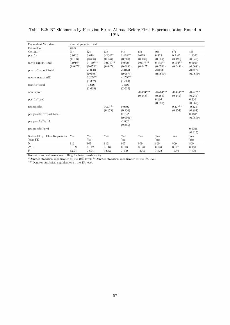
Table B.2: N◦ Shipments by Peruvian Firms Abroad Before First Experimentation Round inUSA

Dependent Variable num shipments totalEstimation OLSColumn (1) (2) (3) (4) (5) (6) (7) (8)

postfta 0.0426 0.618 0.264** 1.428** 0.0294 0.523 0.240* 1.102*(0.108) (0.608) (0.126) (0.710) (0.108) (0.589) (0.126) (0.640)

mean export total 0.0895* 0.140*** 0.0949** 0.0624 0.0973** 0.138** 0.102** 0.0609(0.0473) (0.0536) (0.0478) (0.0682) (0.0477) (0.0541) (0.0481) (0.0681)

postfta*export total -0.0904 -0.0141 -0.0930 -0.0174(0.0599) (0.0674) (0.0600) (0.0669)

new wmean tariff 3.205** 4.155**(1.392) (1.813)

postfta*tariff -0.646 -1.546(1.638) (2.035)

new wpref -0.453*** -0.514*** -0.434*** -0.542**(0.148) (0.189) (0.146) (0.245)

postfta*pref 0.196 0.220(0.220) (0.269)

pre postfta 0.397** 0.0602 0.377** -0.225(0.155) (0.930) (0.154) (0.881)

pre postfta*export total 0.164* 0.160*(0.0901) (0.0899)

pre postfta*tariff -1.802(2.315)

pre postfta*pref 0.0796(0.315)

Sector FE / Other Regressors Yes Yes Yes Yes Yes Yes Yes YesYear FE Yes Yes Yes Yes

N 813 807 813 807 809 809 809 809r2 o 0.109 0.142 0.116 0.148 0.120 0.146 0.127 0.150F 13.24 7.624 12.43 7.499 13.45 7.872 12.59 7.779

Robust standard errors controlling for heteroskedasticity.*Denotes statistical significance at the 10% level; **Denotes statistical significance at the 5% level;***Denotes statistical significance at the 1% level.

57

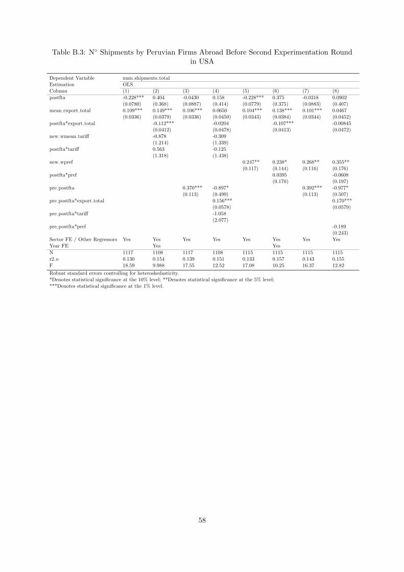
Table B.3: N◦ Shipments by Peruvian Firms Abroad Before Second Experimentation Roundin USA

Dependent Variable num shipments totalEstimation OLSColumn (1) (2) (3) (4) (5) (6) (7) (8)

postfta -0.228*** 0.404 -0.0430 0.158 -0.228*** 0.375 -0.0318 0.0902(0.0780) (0.368) (0.0887) (0.414) (0.0779) (0.375) (0.0883) (0.407)

mean export total 0.109*** 0.149*** 0.106*** 0.0650 0.104*** 0.138*** 0.101*** 0.0467(0.0336) (0.0379) (0.0336) (0.0450) (0.0343) (0.0384) (0.0344) (0.0452)

postfta*export total -0.112*** -0.0204 -0.107*** -0.00845(0.0412) (0.0478) (0.0413) (0.0472)

new wmean tariff -0.878 -0.309(1.214) (1.339)

postfta*tariff 0.563 -0.125(1.318) (1.438)

new wpref 0.247** 0.238* 0.268** 0.355**(0.117) (0.144) (0.116) (0.176)

postfta*pref 0.0395 -0.0608(0.170) (0.197)

pre postfta 0.370*** -0.897* 0.392*** -0.977*(0.113) (0.499) (0.113) (0.507)

pre postfta*export total 0.156*** 0.170***(0.0578) (0.0579)

pre postfta*tariff -1.058(2.077)

pre postfta*pref -0.189(0.243)

Sector FE / Other Regressors Yes Yes Yes Yes Yes Yes Yes YesYear FE Yes Yes

N 1117 1108 1117 1108 1115 1115 1115 1115r2 o 0.130 0.154 0.139 0.151 0.133 0.157 0.143 0.155F 18.59 9.988 17.55 12.52 17.08 10.25 16.37 12.82

Robust standard errors controlling for heteroskedasticity.*Denotes statistical significance at the 10% level; **Denotes statistical significance at the 5% level;***Denotes statistical significance at the 1% level.

58

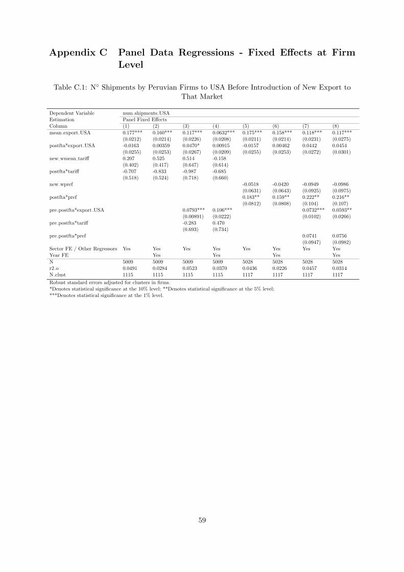
Appendix C Panel Data Regressions - Fixed Effects at FirmLevel

Table C.1: N◦ Shipments by Peruvian Firms to USA Before Introduction of New Export toThat Market

Dependent Variable num shipments USAEstimation Panel Fixed EffectsColumn (1) (2) (3) (4) (5) (6) (7) (8)

mean export USA 0.177*** 0.160*** 0.117*** 0.0632*** 0.175*** 0.158*** 0.118*** 0.117***(0.0212) (0.0214) (0.0226) (0.0208) (0.0211) (0.0214) (0.0231) (0.0275)

postfta*export USA -0.0163 0.00359 0.0470* 0.00915 -0.0157 0.00462 0.0442 0.0454(0.0255) (0.0253) (0.0267) (0.0209) (0.0255) (0.0253) (0.0272) (0.0301)

new wmean tariff 0.207 0.525 0.514 -0.158(0.402) (0.417) (0.647) (0.614)

postfta*tariff -0.707 -0.833 -0.987 -0.685(0.518) (0.524) (0.718) (0.660)

new wpref -0.0518 -0.0420 -0.0949 -0.0986(0.0631) (0.0643) (0.0925) (0.0975)

postfta*pref 0.183** 0.159** 0.222** 0.216**(0.0812) (0.0808) (0.104) (0.107)

pre postfta*export USA 0.0793*** 0.106*** 0.0732*** 0.0593**(0.00891) (0.0222) (0.0102) (0.0266)

pre postfta*tariff -0.283 0.470(0.693) (0.734)

pre postfta*pref 0.0741 0.0756(0.0947) (0.0982)

Sector FE / Other Regressors Yes Yes Yes Yes Yes Yes Yes YesYear FE Yes Yes Yes Yes

N 5009 5009 5009 5009 5028 5028 5028 5028r2 o 0.0491 0.0284 0.0523 0.0370 0.0436 0.0226 0.0457 0.0314N clust 1115 1115 1115 1115 1117 1117 1117 1117

Robust standard errors adjusted for clusters in firms.*Denotes statistical significance at the 10% level; **Denotes statistical significance at the 5% level;***Denotes statistical significance at the 1% level.

59

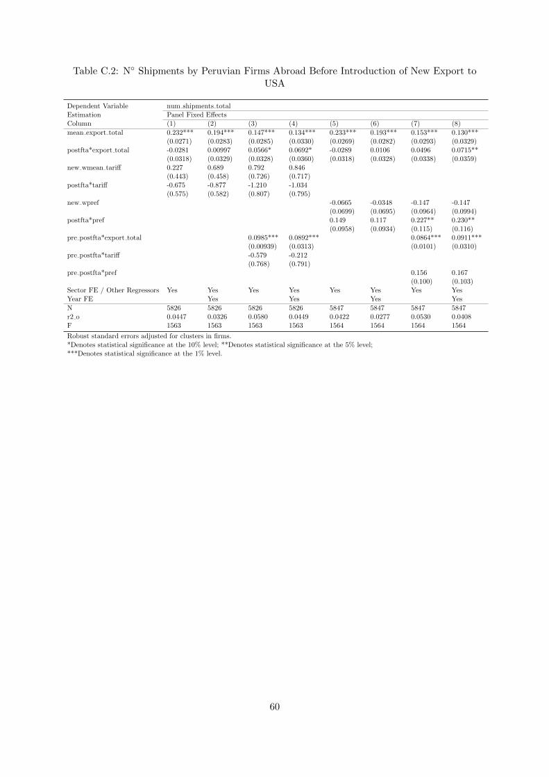
Table C.2: N◦ Shipments by Peruvian Firms Abroad Before Introduction of New Export toUSA

Dependent Variable num shipments totalEstimation Panel Fixed EffectsColumn (1) (2) (3) (4) (5) (6) (7) (8)

mean export total 0.232*** 0.194*** 0.147*** 0.134*** 0.233*** 0.193*** 0.153*** 0.130***(0.0271) (0.0283) (0.0285) (0.0330) (0.0269) (0.0282) (0.0293) (0.0329)

postfta*export total -0.0281 0.00997 0.0566* 0.0692* -0.0289 0.0106 0.0496 0.0715**(0.0318) (0.0329) (0.0328) (0.0360) (0.0318) (0.0328) (0.0338) (0.0359)

new wmean tariff 0.227 0.689 0.792 0.846(0.443) (0.458) (0.726) (0.717)

postfta*tariff -0.675 -0.877 -1.210 -1.034(0.575) (0.582) (0.807) (0.795)

new wpref -0.0665 -0.0348 -0.147 -0.147(0.0699) (0.0695) (0.0964) (0.0994)

postfta*pref 0.149 0.117 0.227** 0.230**(0.0958) (0.0934) (0.115) (0.116)

pre postfta*export total 0.0985*** 0.0892*** 0.0864*** 0.0911***(0.00939) (0.0313) (0.0101) (0.0310)

pre postfta*tariff -0.579 -0.212(0.768) (0.791)

pre postfta*pref 0.156 0.167(0.100) (0.103)

Sector FE / Other Regressors Yes Yes Yes Yes Yes Yes Yes YesYear FE Yes Yes Yes Yes

N 5826 5826 5826 5826 5847 5847 5847 5847r2 o 0.0447 0.0326 0.0580 0.0449 0.0422 0.0277 0.0530 0.0408F 1563 1563 1563 1563 1564 1564 1564 1564

Robust standard errors adjusted for clusters in firms.*Denotes statistical significance at the 10% level; **Denotes statistical significance at the 5% level;***Denotes statistical significance at the 1% level.

60

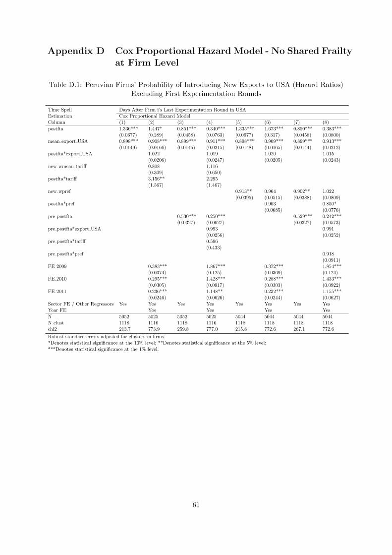
Appendix D Cox Proportional Hazard Model - No Shared Frailtyat Firm Level

Table D.1: Peruvian Firms’ Probability of Introducing New Exports to USA (Hazard Ratios)Excluding First Experimentation Rounds

Time Spell Days After Firm i’s Last Experimentation Round in USAEstimation Cox Proportional Hazard ModelColumn (1) (2) (3) (4) (5) (6) (7) (8)

postfta 1.336*** 1.447* 0.851*** 0.340*** 1.335*** 1.673*** 0.850*** 0.383***(0.0677) (0.289) (0.0458) (0.0763) (0.0677) (0.317) (0.0458) (0.0800)

mean export USA 0.898*** 0.908*** 0.899*** 0.911*** 0.898*** 0.909*** 0.899*** 0.913***(0.0149) (0.0166) (0.0145) (0.0215) (0.0148) (0.0165) (0.0144) (0.0212)

postfta*export USA 1.022 1.019 1.020 1.015(0.0206) (0.0247) (0.0205) (0.0243)

new wmean tariff 0.808 1.116(0.309) (0.650)

postfta*tariff 3.156** 2.295(1.567) (1.467)

new wpref 0.913** 0.964 0.902** 1.022(0.0395) (0.0515) (0.0388) (0.0809)

postfta*pref 0.903 0.850*(0.0685) (0.0776)

pre postfta 0.530*** 0.250*** 0.529*** 0.242***(0.0327) (0.0627) (0.0327) (0.0573)

pre postfta*export USA 0.993 0.991(0.0256) (0.0252)

pre postfta*tariff 0.596(0.433)

pre postfta*pref 0.918(0.0911)

FE 2009 0.383*** 1.867*** 0.372*** 1.854***(0.0374) (0.125) (0.0369) (0.124)

FE 2010 0.295*** 1.428*** 0.288*** 1.433***(0.0305) (0.0917) (0.0303) (0.0922)

FE 2011 0.236*** 1.148** 0.232*** 1.155***(0.0246) (0.0626) (0.0244) (0.0627)

Sector FE / Other Regressors Yes Yes Yes Yes Yes Yes Yes YesYear FE Yes Yes Yes Yes

N 5052 5025 5052 5025 5044 5044 5044 5044N clust 1118 1116 1118 1116 1118 1118 1118 1118chi2 213.7 773.9 259.8 777.0 215.8 772.6 267.1 772.6

Robust standard errors adjusted for clusters in firms.*Denotes statistical significance at the 10% level; **Denotes statistical significance at the 5% level;***Denotes statistical significance at the 1% level.

61

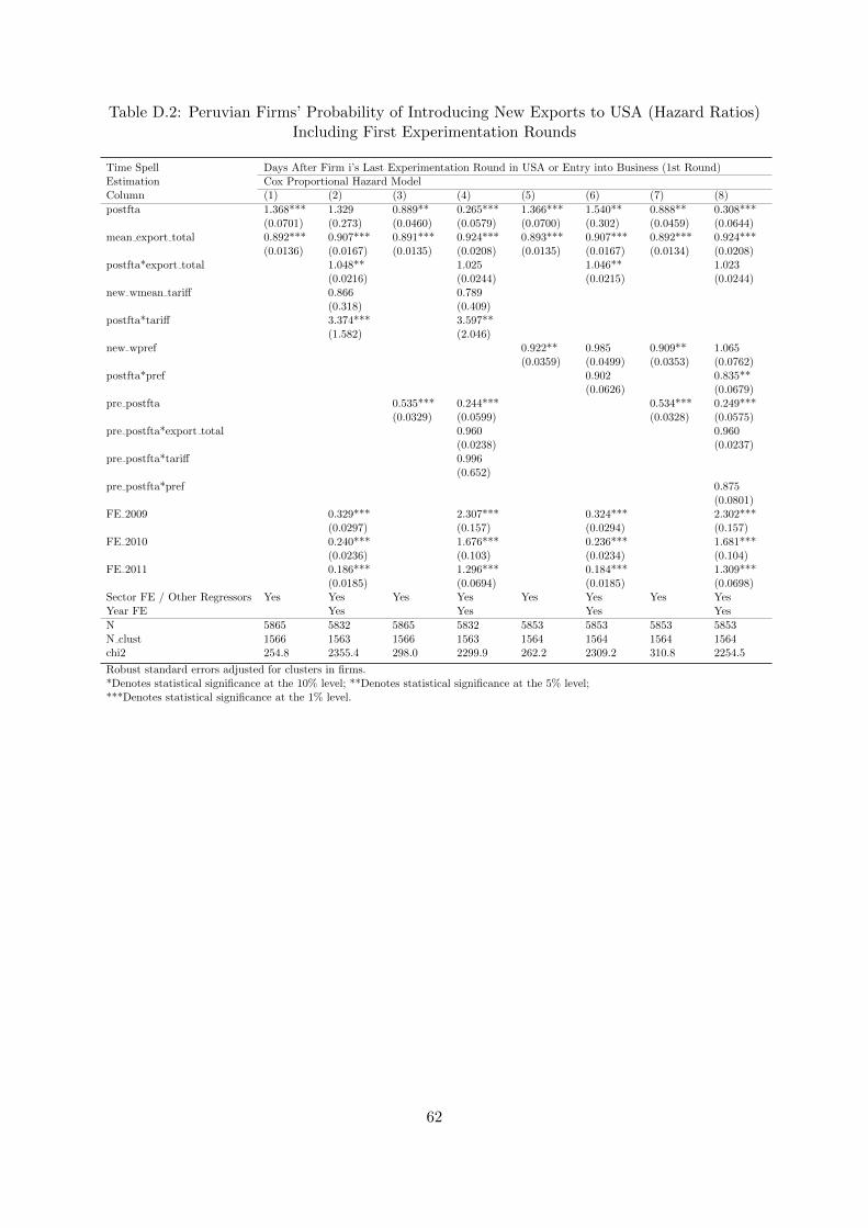
Table D.2: Peruvian Firms’ Probability of Introducing New Exports to USA (Hazard Ratios)Including First Experimentation Rounds

Time Spell Days After Firm i’s Last Experimentation Round in USA or Entry into Business (1st Round)Estimation Cox Proportional Hazard ModelColumn (1) (2) (3) (4) (5) (6) (7) (8)

postfta 1.368*** 1.329 0.889** 0.265*** 1.366*** 1.540** 0.888** 0.308***(0.0701) (0.273) (0.0460) (0.0579) (0.0700) (0.302) (0.0459) (0.0644)

mean export total 0.892*** 0.907*** 0.891*** 0.924*** 0.893*** 0.907*** 0.892*** 0.924***(0.0136) (0.0167) (0.0135) (0.0208) (0.0135) (0.0167) (0.0134) (0.0208)

postfta*export total 1.048** 1.025 1.046** 1.023(0.0216) (0.0244) (0.0215) (0.0244)

new wmean tariff 0.866 0.789(0.318) (0.409)

postfta*tariff 3.374*** 3.597**(1.582) (2.046)

new wpref 0.922** 0.985 0.909** 1.065(0.0359) (0.0499) (0.0353) (0.0762)

postfta*pref 0.902 0.835**(0.0626) (0.0679)

pre postfta 0.535*** 0.244*** 0.534*** 0.249***(0.0329) (0.0599) (0.0328) (0.0575)

pre postfta*export total 0.960 0.960(0.0238) (0.0237)

pre postfta*tariff 0.996(0.652)

pre postfta*pref 0.875(0.0801)

FE 2009 0.329*** 2.307*** 0.324*** 2.302***(0.0297) (0.157) (0.0294) (0.157)

FE 2010 0.240*** 1.676*** 0.236*** 1.681***(0.0236) (0.103) (0.0234) (0.104)

FE 2011 0.186*** 1.296*** 0.184*** 1.309***(0.0185) (0.0694) (0.0185) (0.0698)

Sector FE / Other Regressors Yes Yes Yes Yes Yes Yes Yes YesYear FE Yes Yes Yes Yes

N 5865 5832 5865 5832 5853 5853 5853 5853N clust 1566 1563 1566 1563 1564 1564 1564 1564chi2 254.8 2355.4 298.0 2299.9 262.2 2309.2 310.8 2254.5

Robust standard errors adjusted for clusters in firms.*Denotes statistical significance at the 10% level; **Denotes statistical significance at the 5% level;***Denotes statistical significance at the 1% level.

62

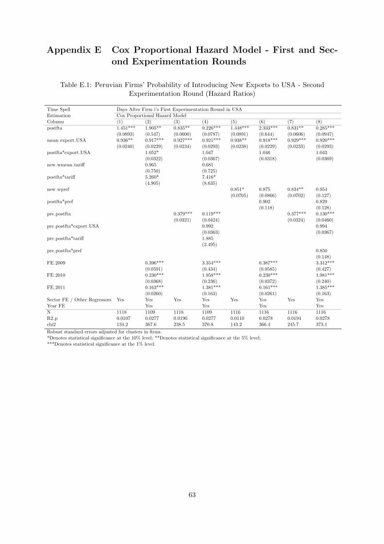
Appendix E Cox Proportional Hazard Model - First and Sec-ond Experimentation Rounds

Table E.1: Peruvian Firms’ Probability of Introducing New Exports to USA - SecondExperimentation Round (Hazard Ratios)

Time Spell Days After Firm i’s First Experimentation Round in USAEstimation Cox Proportional Hazard ModelColumn (1) (2) (3) (4) (5) (6) (7) (8)

postfta 1.451*** 1.905** 0.835** 0.226*** 1.448*** 2.333*** 0.831** 0.285***(0.0893) (0.547) (0.0600) (0.0787) (0.0891) (0.644) (0.0606) (0.0947)

mean export USA 0.936** 0.917*** 0.927*** 0.921*** 0.938** 0.918*** 0.929*** 0.920***(0.0240) (0.0229) (0.0234) (0.0293) (0.0238) (0.0229) (0.0233) (0.0293)

postfta*export USA 1.052* 1.047 1.046 1.043(0.0322) (0.0367) (0.0318) (0.0369)

new wmean tariff 0.965 0.681(0.750) (0.725)

postfta*tariff 5.260* 7.416*(4.905) (8.635)

new wpref 0.851* 0.875 0.834** 0.954(0.0705) (0.0866) (0.0702) (0.127)

postfta*pref 0.902 0.829(0.118) (0.128)

pre postfta 0.379*** 0.119*** 0.377*** 0.130***(0.0321) (0.0424) (0.0324) (0.0460)

pre postfta*export USA 0.992 0.994(0.0363) (0.0367)

pre postfta*tariff 1.885(2.495)

pre postfta*pref 0.850(0.148)

FE 2009 0.396*** 3.354*** 0.387*** 3.312***(0.0591) (0.434) (0.0585) (0.427)

FE 2010 0.230*** 1.958*** 0.230*** 1.981***(0.0368) (0.236) (0.0372) (0.240)

FE 2011 0.163*** 1.381*** 0.161*** 1.385***(0.0260) (0.163) (0.0261) (0.163)

Sector FE / Other Regressors Yes Yes Yes Yes Yes Yes Yes YesYear FE Yes Yes Yes Yes

N 1118 1109 1118 1109 1116 1116 1116 1116R2 p 0.0107 0.0277 0.0190 0.0277 0.0110 0.0278 0.0194 0.0278chi2 134.2 367.6 238.5 370.8 143.2 366.4 245.7 373.1

Robust standard errors adjusted for clusters in firms.*Denotes statistical significance at the 10% level; **Denotes statistical significance at the 5% level;***Denotes statistical significance at the 1% level.

63

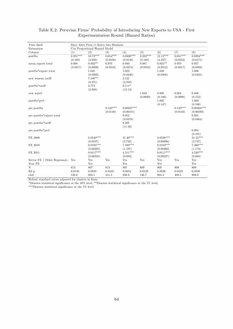
Table E.2: Peruvian Firms’ Probability of Introducing New Exports to USA - FirstExperimentation Round (Hazard Ratios)

Time Spell Days After Firm i’s Entry into BusinessEstimation Cox Proportional Hazard ModelColumn (1) (2) (3) (4) (5) (6) (7) (8)

postfta 2.291*** 10.73*** 0.654*** 0.0300*** 2.282*** 12.12*** 0.651*** 0.0394***(0.169) (3.956) (0.0550) (0.0138) (0.169) (4.227) (0.0553) (0.0171)

mean export total 0.988 0.922** 0.970 0.940 0.987 0.925** 0.970 0.957(0.0317) (0.0309) (0.0316) (0.0374) (0.0316) (0.0312) (0.0317) (0.0393)

postfta*export total 1.045 1.023 1.039 1.006(0.0393) (0.0436) (0.0388) (0.0431)

new wmean tariff 7.108** 2.121(6.271) (2.583)

postfta*tariff 2.773 9.111*(2.928) (12.13)

new wpref 1.023 0.886 0.964 0.886(0.0949) (0.109) (0.0998) (0.152)

postfta*pref 1.002 1.003(0.147) (0.186)

pre postfta 0.133*** 0.00337*** 0.133*** 0.00464***(0.0140) (0.00181) (0.0140) (0.00239)

pre postfta*export total 0.952 0.931(0.0476) (0.0464)

pre postfta*tariff 8.207(11.56)

pre postfta*pref 0.994(0.191)

FE 2009 0.0549*** 21.30*** 0.0526*** 21.55***(0.0107) (3.732) (0.00998) (3.747)

FE 2010 0.0195*** 7.580*** 0.0183*** 7.460***(0.00395) (1.197) (0.00360) (1.173)

FE 2011 0.0117*** 4.511*** 0.0111*** 4.520***(0.00245) (0.693) (0.00227) (0.694)

Sector FE / Other Regressors Yes Yes Yes Yes Yes Yes Yes YesYear FE Yes Yes Yes Yes

N 813 807 813 807 809 809 809 809R2 p 0.0140 0.0849 0.0423 0.0852 0.0138 0.0836 0.0423 0.0838chi2 138.6 934.1 411.5 938.8 136.7 904.4 409.5 908.0

Robust standard errors adjusted for clusters in firms.*Denotes statistical significance at the 10% level; **Denotes statistical significance at the 5% level;***Denotes statistical significance at the 1% level.

64

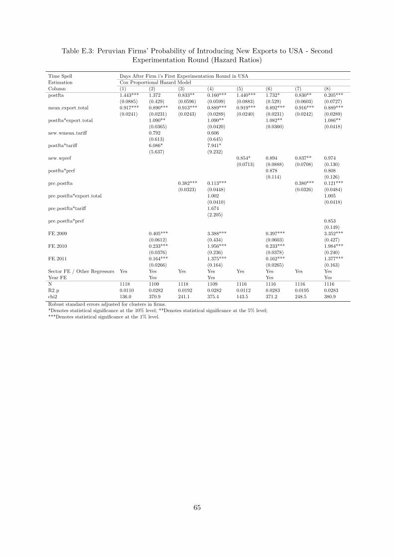
Table E.3: Peruvian Firms’ Probability of Introducing New Exports to USA - SecondExperimentation Round (Hazard Ratios)

Time Spell Days After Firm i’s First Experimentation Round in USAEstimation Cox Proportional Hazard ModelColumn (1) (2) (3) (4) (5) (6) (7) (8)

postfta 1.443*** 1.372 0.833** 0.160*** 1.440*** 1.732* 0.830** 0.205***(0.0885) (0.429) (0.0596) (0.0599) (0.0883) (0.529) (0.0603) (0.0727)

mean export total 0.917*** 0.890*** 0.913*** 0.889*** 0.919*** 0.892*** 0.916*** 0.889***(0.0241) (0.0231) (0.0243) (0.0289) (0.0240) (0.0231) (0.0242) (0.0289)

postfta*export total 1.090** 1.090** 1.082** 1.086**(0.0365) (0.0420) (0.0360) (0.0418)

new wmean tariff 0.792 0.606(0.613) (0.645)

postfta*tariff 6.086* 7.941*(5.637) (9.232)

new wpref 0.854* 0.894 0.837** 0.974(0.0713) (0.0888) (0.0708) (0.130)

postfta*pref 0.878 0.808(0.114) (0.126)

pre postfta 0.382*** 0.113*** 0.380*** 0.121***(0.0323) (0.0448) (0.0326) (0.0484)

pre postfta*export total 1.002 1.005(0.0410) (0.0418)

pre postfta*tariff 1.674(2.205)

pre postfta*pref 0.853(0.149)

FE 2009 0.405*** 3.388*** 0.397*** 3.352***(0.0612) (0.434) (0.0603) (0.427)

FE 2010 0.233*** 1.956*** 0.233*** 1.984***(0.0376) (0.236) (0.0378) (0.240)

FE 2011 0.164*** 1.375*** 0.162*** 1.377***(0.0266) (0.164) (0.0265) (0.163)

Sector FE / Other Regressors Yes Yes Yes Yes Yes Yes Yes YesYear FE Yes Yes Yes Yes

N 1118 1109 1118 1109 1116 1116 1116 1116R2 p 0.0110 0.0282 0.0192 0.0282 0.0112 0.0283 0.0195 0.0283chi2 136.0 370.9 241.1 375.4 143.5 371.2 248.5 380.9

Robust standard errors adjusted for clusters in firms.*Denotes statistical significance at the 10% level; **Denotes statistical significance at the 5% level;***Denotes statistical significance at the 1% level.

65