Experimental Verification of a Wireless Sensing and Control System for Structural Control Using MR-Dampers

Chin-Hsiung Loh1, Jerome P. Lynch2, Kung-Chun Lu1, Yang Wang3

Chia-Ming Chang1, Pei-Yang Lin4, Ting-Hei Yeh1

ABSTRACT

The performance aspects of a wireless “active” sensor, including the reliability of the wireless

communication channel for real-time data delivery and its application to feedback structural

control, are explored in this study. First, the control of magnetorheological (MR) dampers

using wireless sensors is examined. Second, the application of the MR-damper to actively

control a half-scale three-story steel building excited at its base by shaking table is studied

using a wireless control system assembled from wireless active sensors. With an MR damper

installed on each floor (3 dampers total), structural responses during seismic excitation are

measured by the system’s wireless active sensors and wirelessly communicated to each other;

upon receipt of response data, the wireless sensor interfaced to each MR damper calculates a

desired control action using an LQG controller implemented in the wireless sensor’s

computational core. In this system, the wireless active sensor is responsible for the reception

of response data, determination of optimal control forces, and the issuing of command signals

to the MR damper. Various control solutions are formulated in this study and embedded in

the wireless control system including centralized and decentralized control algorithms.

Keywords: Wireless active sensor, LQG control algorithm, MR-damper, decentralized control.

1 Department of Civil Engineering, National Taiwan University, Taipei 106-17, Taiwan 2 Department of Civil & Environmental Engineering, University of Michigan, Ann Arbor, USA 3 Department of Civil & Environmental Engineering, Stanford University, Stanford, USA 4 National Center for Research on Earthquake Engineering, Taipei, Taiwan

Experimental Verification of a Wireless Sensing and Control System for Structural Control Using MR-Dampers

Chin-Hsiung Loh1, Jerome P. Lynch2, Kung-Chun Lu1, Yang Wang4

Chia-Ming Chang1, Pei-Yang Lin3, Ting-Hei Yeh1

1. INTRODUCTION

For the installation of semi-active control devices (magnetorheological (MR) dampers) in

structures, extensive lengths of wires are often needed to connect sensors (to provide real-time

state feedback) with a controller where control forces are calculated. In contrast to this

classical approach, wireless sensors can be considered for controlling structures. In order to

reduce the monetary and time expenses associated with the installation of wire-based systems,

the emergence of new embedded system and wireless communication technologies have been

adopted in academia and industry for wireless monitoring. The use of wireless communications

within a structural health monitoring (SHM) data acquisition system was illustrated by Straser

and Kiremidjian [1998]. More recently, Lynch et al. have extended upon this work by

embedding damage identification algorithms into the wireless sensors [Lynch et al. 2004] and

have proven the reliability of the system in harsh field conditions [Wang et al. 2005; Lynch et

al. 2005; Lynch et al. 2006a]. While the advantages of using wireless sensors for structural

health monitoring have been verified in the structural monitoring area, many challenges must

still be explored in greater detail before they can be adopted for structural control.

To dissipate hysteretic energy and to indirectly apply control forces to a civil structure,

semi-active control devices, like MR dampers, have been developed and applied to various

structures in recent years [Dyke et al., 1996; Spencer et al., 1999; Yang et al., 2002; Occhiuzzi

et al., 2003, Spencer and Nagarajaiah 2003; Nishitani et al. 2003; Kurino et al. 2003]. The

voltage-dependent nonlinear hysteretic behavior allows MR dampers to be very flexible in

resisting different levels of external force. A number of control studies have thoroughly

investigated and modeled the command-force relationships for MR dampers [Dyke et al., 1996].

Several analytical and experimental studies focues upon the seismic protection of structures

using MR dampers have also been published [Lin et al., 2002, 2004]. An inclusive goal of

this study is to further validate the effectiveness of MR dampers in the application of structural

control. A prototype wireless structural sensing and control system has been previously

proposed [Lynch et al. 2006b] for structural response mitigation. The software written to

operate the wireless sensors under the real-time requirements of the control problem is

presented in detail herein. The promising performance of wireless communication and

embedded computing technology within a real-time feedback structural control system is

offered.

This paper presents the experimental verification of using both fully centralized control

and fully decentralized control strategies within a structural control system assembled from

semi-active control devices (MR dampers) and a wireless sensor network consisting of wireless

sensors capable of actuation. An almost full-scale three-story steel building with MR

dampers installed upon each floor of the structure is tested by applying base motion using a 6

degree-of-freedom (DOF) shaking table. Structural responses are measured during seismic

excitation by the wireless sensors and wirelessly communicated to wireless sensors interfaced

to the system’s MR damper. Embedded within each wireless sensor’s computational core is

an LQG control solution. Specifically, two major research directions are emphasized in this

study:

1. The theoretical basis for fully centralized and fully decentralized control algorithms are

offered for implementation within a wireless structural control system.

2. Experimental verification of wireless communications for real-time structural control is

made and comparison of the control performance of the wireless control system is compared

to that of a traditional tethered control system.

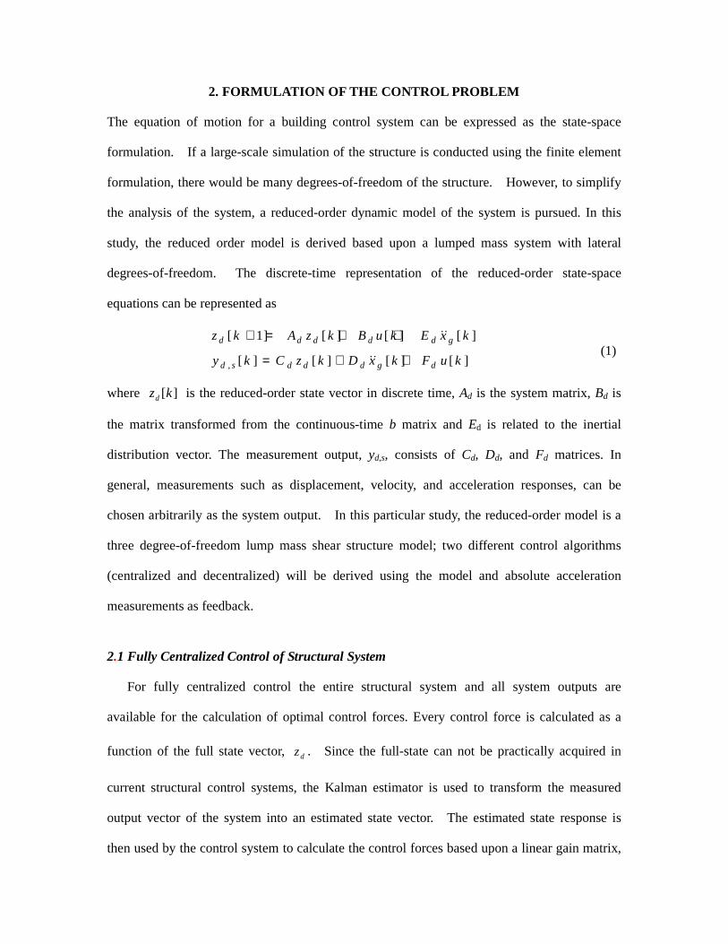
2. FORMULATION OF THE CONTROL PROBLEM

The equation of motion for a building control system can be expressed as the state-space

formulation. If a large-scale simulation of the structure is conducted using the finite element

formulation, there would be many degrees-of-freedom of the structure. However, to simplify

the analysis of the system, a reduced-order dynamic model of the system is pursued. In this

study, the reduced order model is derived based upon a lumped mass system with lateral

degrees-of-freedom. The discrete-time representation of the reduced-order state-space

equations can be represented as

,

[ 1] [ ] [ ] [ ]

[ ] [ ] [ ] [ ]

d d d d d g

d s d d d g d

z k A z k B u k E x k

y k C z k D x k F u k

+ = + +

= + +

ɺɺ

ɺɺ (1)

where ][kzd is the reduced-order state vector in discrete time, Ad is the system matrix, Bd is

the matrix transformed from the continuous-time b matrix and Ed is related to the inertial

distribution vector. The measurement output, yd,s, consists of Cd, Dd, and Fd matrices. In

general, measurements such as displacement, velocity, and acceleration responses, can be

chosen arbitrarily as the system output. In this particular study, the reduced-order model is a

three degree-of-freedom lump mass shear structure model; two different control algorithms

(centralized and decentralized) will be derived using the model and absolute acceleration

measurements as feedback.

2.1 Fully Centralized Control of Structural System

For fully centralized control the entire structural system and all system outputs are

available for the calculation of optimal control forces. Every control force is calculated as a

function of the full state vector, dz . Since the full-state can not be practically acquired in

current structural control systems, the Kalman estimator is used to transform the measured

output vector of the system into an estimated state vector. The estimated state response is

then used by the control system to calculate the control forces based upon a linear gain matrix,

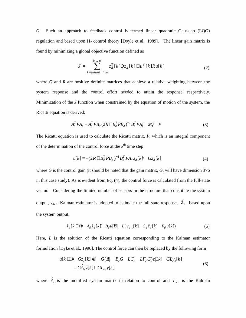
G. Such an approach to feedback control is termed linear quadratic Gaussian (LQG)

regulation and based upon H2 control theory [Doyle et al., 1989]. The linear gain matrix is

found by minimizing a global objective function defined as

[ ] [ ] [ ] [ ]k

T Td d

k initail time

J z k Qz k u k Ru k→ ∞

=

= +∑ (2)

where Q and R are positive definite matrices that achieve a relative weighting between the

system response and the control effort needed to attain the response, respectively.

Minimization of the J function when constrained by the equation of motion of the system, the

Ricatti equation is derived:

1(2 ) 2T T T Td d d d d d d dA PA A PB R B PB B PA Q P−− + + = (3)

The Ricatti equation is used to calculate the Ricatti matrix, P, which is an integral component

of the determination of the control force at the kth time step

1[ ] (2 ) [ ] [ ]T Td d d d d du k R B PB B PA z k Gz k−= − + = (4)

where G is the control gain (it should be noted that the gain matrix, G, will have dimension 3×6

in this case study). As is evident from Eq. (4), the control force is calculated from the full-state

vector. Considering the limited number of sensors in the structure that constitute the system

output, yd, a Kalman estimator is adopted to estimate the full state response, dz , based upon

the system output:

,[ 1] [ ] [ ] ( [ ] [ ] [ ])d d d d d s d d dz k A z k B u k L y k C z k F u k+ = + + − −⌢ ⌢ ⌢ (5)

Here, L is the solution of the Ricatti equation corresponding to the Kalman estimator

formulation [Dyke et al., 1996]. The control force can then be replaced by the following form

[ 1] [ 1] ( ) [ ] [ ]

ˆ ˆ[ ] [ ]

d d d c d d d

cs ms

u k Gz k G A B G LC LF G z k GLy k

GA z k GL y k

+ = + = + − − +

= + (6)

where csA is the modified system matrix in relation to control and msL is the Kalman

estimator in relation to the system measurements. As is seen in Eq. (6), the control force is

generated using the full state response vector. Since each actuator (which corresponds to each

row of the gain matrix) requires the full state response to determine its control action, this

control approach assumes a fully centralized control architecture.

2.2 Fully Decentralized Control of Structural System

Fully decentralized control emphasizes control of the local sub-system only using the

sub-system’s actuators and sensor measurements. It is to mitigate the response of the

structure using limited information (partial state information) and independent controllers

corresponding to sub-systems of the global structure. The control force generated by a

sub-system controller would inherently be independent from those of the other sub-systems.

A main advantage of decentralized control architectures is that subsystem controllers are

independent; the malfunction of an individual controller will not cause the failure of whole

control system. In exchange for the reliability offered by decentralized control methods is

that their control performance is below that of their centralized counterparts. Within the

structural control community, a number of researchers have explored decentralized approaches

to the complex control problem [Nishitani et al. 2003; Kurino et al. 2003].

To formulate a decentralized control solution, the discrete time state-space equation is

rewritten as

, ,

[ 1] [ ] ( ) [ ] [ ]

( ) [ ] ( ) [ ] ( ) [ ] ( ) [ ]

d d d d i i d g

d s j d j d d j g d j i i

z k A z k B u k E x k

y k C z k D x k F u k

+ = + +

= + +

∑∑

ɺɺ

ɺɺ (7)

where “j” indicates j-th subsystem and “I” indicates i-th locations of actuator, and yj indicates

the measured output of the jth sub-system of the measurement system. Let it be assumed that

for each subsystem, there is one control actuator which applies a control force. The control

force of the ith actuator is denoted as ui and its control action seeks to minimize the following

objective function:

[ ] [ ] [ ] [ ]k

T Ti d d i i

k initail time

J z k Qz k u k Ru k→∞

=

= +∑⌢

(8)

Here, R⌢

is a scalar weighting term and may be different for each actuator depending upon the

objectives of the specific actuator. The number of objective functions is the same as the

number of subsystems defined in the global structure.

Consider a three-story structure where each floor is considered a subsystem within the

control system. If an actuator and sensor (measuring acceleration) are collocated upon each

floor of the structure, each floor can be considered its own subsystem. Provided three

sub-systems, the global state-space equation and the measurement output equations

corresponding to each subsystem (i.e. floor) can be written:

3

1

3

1 ,1 1 6 ,11 1 1 1 ,1 1 1 ,1 1 12

2 ,2 1 6 ,22 1 1 2 ,2 1 1 ,2 1 11,3

3 ,

[ 1] [ ] ( ) [ ] [ ]

[ ] ( ) [ ] ( ) [ ] ( ) [ ] ( ) [ ]

[ ] ( ) [ ] ( ) [ ] ( ) [ ] ( ) [ ]

[ ] (

d d d d i i d gi

d d d d j j d gj

d d d d j j d gj

d

z k A z k B u k E x k

y k C z k D u k D u k F x k

y k C z k D u k D u k F x k

y k C

=

× × × ×=

× × × ×=

+ = + +

= + + +

= + + +

=

∑

∑

∑

ɺɺ

ɺɺ

ɺɺ

2

3 1 6 ,33 1 1 3 ,3 1 1 ,3 1 11

) [ ] ( ) [ ] ( ) [ ] ( ) [ ]d d d j j d gj

z k D u k D u k F x k× × × ×=

+ + +∑ ɺɺ

(9)

Here, the matrix (Cd,1)1x6 corresponds to the 1st row (with dimensions 1 by 6) of the

discrete-time matrix dC of Eq. (4); the other matrix notations follows the same convention.

The objective function, Ji, for the ith floor can be written for all three floors:

1 6 6 1 1 1 10

2 6 6 2 1 1 20

3 6 6 3 1 1 30

[ ] [ ] [ ] [ ]

[ ] [ ] [ ] [ ]

[ ] [ ] [ ] [ ]

T Td d

k

T Td d

k

T Td d

k

J z k Q z k u k R u k

J z k Q z k u k R u k

J z k Q z k u k R u k

∞

× ×=

∞

× ×=

∞

× ×=

= +

= +

= +

∑

∑

∑

⌢

⌢

⌢

(10)

Each objective function will derive an optimal gain matrix that corresponds to the objectives of

the subsystem actuator. The Ricatti equation derived from the ith sub-system objective

function can be presented:

1, 6 1 1 1 , 6 1 , 6 1( ) (2 ( ) ) ( ) 2T T T T

d d d d i d d i d i dA PA A P B R B P B B PA Q P−× × × ×− + + =⌢

(11)

Based upon the solution of the Ricatti equation, the control gain of the subsystem can be

described:

1, , , 1 6[ ] (2 ) ( ) [ ] ( ) [ ]T T

i d i d i d i d i d iu k R B PB B PA z k G z k−×= − + =

⌢

(12)

It should be noted that the gain matrix relating the full state response to the ith control force, ui,

has the dimensions of 1 by 6. To maintain the fully decentralized architecture, the

communication of response data between the sub-systems does not occur. Therefore, a

Kalman estimator is used to estimate the full state response, dz , based upon the measured

system output:

, ,( ) [ 1] [ ] ( ) [ ] (( ) [ ] ( ) ( ) [ ] ( ) [ ])d i d d d i i j d s j d j d i d j i iz k A z k B u k L y k C z k F u k+ = + + − −⌢ ⌢ ⌢ (13)

If control force of Eq. (12) is substituted into Eq. (13), the estimator can be rewritten as

, ,( ) [ 1] ( ( ) ( ) ( ) )( ) [ ] ( ) [ ]d i d d i i j d j j d j i i d i j d s jz k A B G L C L F G z k L y k+ = + − − +⌢ ⌢ (13a)

here subscript i indicates the full state estimated by the i th subsystem Kalman estimator. The

estimated full state is then used to determine the optimal control force to be applied by the

sub-system actuator:

[ 1] ( ) [ 1]i i d iu k G z k+ = +⌢ (14)

3. THE EXPERIMENAL SET-UP

3.1 Test Structure

A three-story half-scale steel structure is designed and constructed at the National Center

for Research on Earthquake Engineering (NCREE) in Taipei, Taiwan. As shown in Figure 1,

the three-story structure consists of a single bay with a 3m by 2m floor area and 3m tall stories.

The structure is constructed using H150x150x7x10 steel I-beam elements with each

beam-column joint designed as a bolted connection. Concrete blocks are added and fastened to

the floor diaphragms until the total mass of each floor is precisely 6,000 kg. The entire

structure is constructed upon a large-scale NCREE shaking table capable of applying base

motion in 6 independent degrees-of-freedom. The structural behavior is modeled using a

lumped mass shear structure reduced-order structural model defined by 3 degrees-of-freedom

(i.e. the lateral displacement of each floor). Based on the response of the bare frame, the

damping and stiffness matrices of a reduced-order model were identified using system

identification techniques. The identified natural frequencies corresponding to the first three

modes of the structure are 1.08, 3.25, and 5.06 Hz, respectively. Furthermore, the damping

ratio of the 1st, 2nd, and 3rd modes are 1.6%, 1.7%, and 2.7%, respectively. The identified

natural frequencies are in consistent with the mathematical model.

3.2 The MR-Damper

The magnetic field that controls the viscosity of the MR fluid is generated by the

application of an electrical current to the coil surrounding the damper chamber. Therefore,

higher damping coefficients can be attained by the MR damper simply by increasing the coil

current. To render the MR damper compatible with a feedback control system, a VCCS

(voltage current converter) unit will be needed to translate voltage command signals to the

electrical current applied to the MR damper coil. In this study, the effects of temperature of

the MR damper are not considered and the voltage-current conversion is assumed linearly

proportional. Three 20 kN MR dampers designed for the purposes of controlling the dynamic

response of the test structure, are constructed. MR dampers are inherently nonlinear devices

that must be properly modeled prior to their use within a control system. Prior study of the

MR dampers constructed reveals the suitability of using a modified Bouc-Wen model to

express their force-velocity functions [Lin et al., 2005]. The total restoring force of the

Bouc-Wen damper model is expressed as:

)()()(~

kxCkzkF ɺ+= (15)

and dtkkkzkzi

ii∑=

−−+−=5

1

)1()1()1()( φθ (15a)

[ ]Tkzkxkzkzkxkzkxkzkzkxkxtk2110

)()(),()()(,)()(),()()(),(*)( ɺɺɺɺɺ∆=φ (15b)

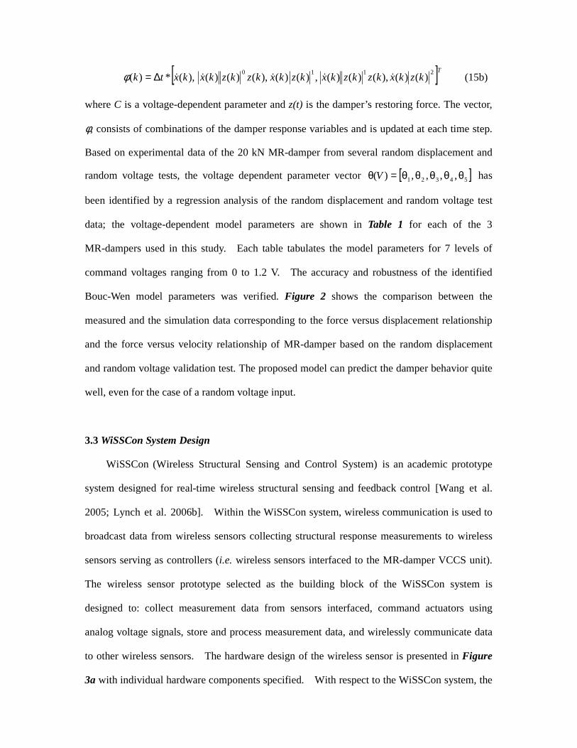
where C is a voltage-dependent parameter and z(t) is the damper’s restoring force. The vector,

φ, consists of combinations of the damper response variables and is updated at each time step.

Based on experimental data of the 20 kN MR-damper from several random displacement and

random voltage tests, the voltage dependent parameter vector [ ]54321 ,,,,)( θθθθθ=θ V has

been identified by a regression analysis of the random displacement and random voltage test

data; the voltage-dependent model parameters are shown in Table 1 for each of the 3

MR-dampers used in this study. Each table tabulates the model parameters for 7 levels of

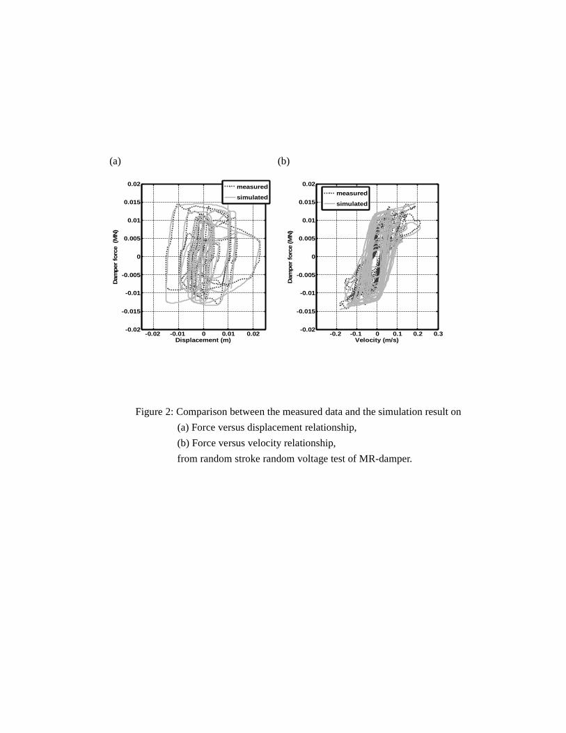
command voltages ranging from 0 to 1.2 V. The accuracy and robustness of the identified

Bouc-Wen model parameters was verified. Figure 2 shows the comparison between the

measured and the simulation data corresponding to the force versus displacement relationship

and the force versus velocity relationship of MR-damper based on the random displacement

and random voltage validation test. The proposed model can predict the damper behavior quite

well, even for the case of a random voltage input.

3.3 WiSSCon System Design

WiSSCon (Wireless Structural Sensing and Control System) is an academic prototype

system designed for real-time wireless structural sensing and feedback control [Wang et al.

2005; Lynch et al. 2006b]. Within the WiSSCon system, wireless communication is used to

broadcast data from wireless sensors collecting structural response measurements to wireless

sensors serving as controllers (i.e. wireless sensors interfaced to the MR-damper VCCS unit).

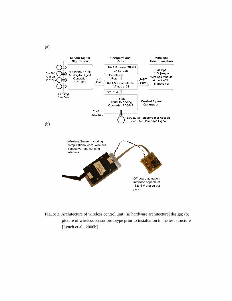
The wireless sensor prototype selected as the building block of the WiSSCon system is

designed to: collect measurement data from sensors interfaced, command actuators using

analog voltage signals, store and process measurement data, and wirelessly communicate data

to other wireless sensors. The hardware design of the wireless sensor is presented in Figure

3a with individual hardware components specified. With respect to the WiSSCon system, the

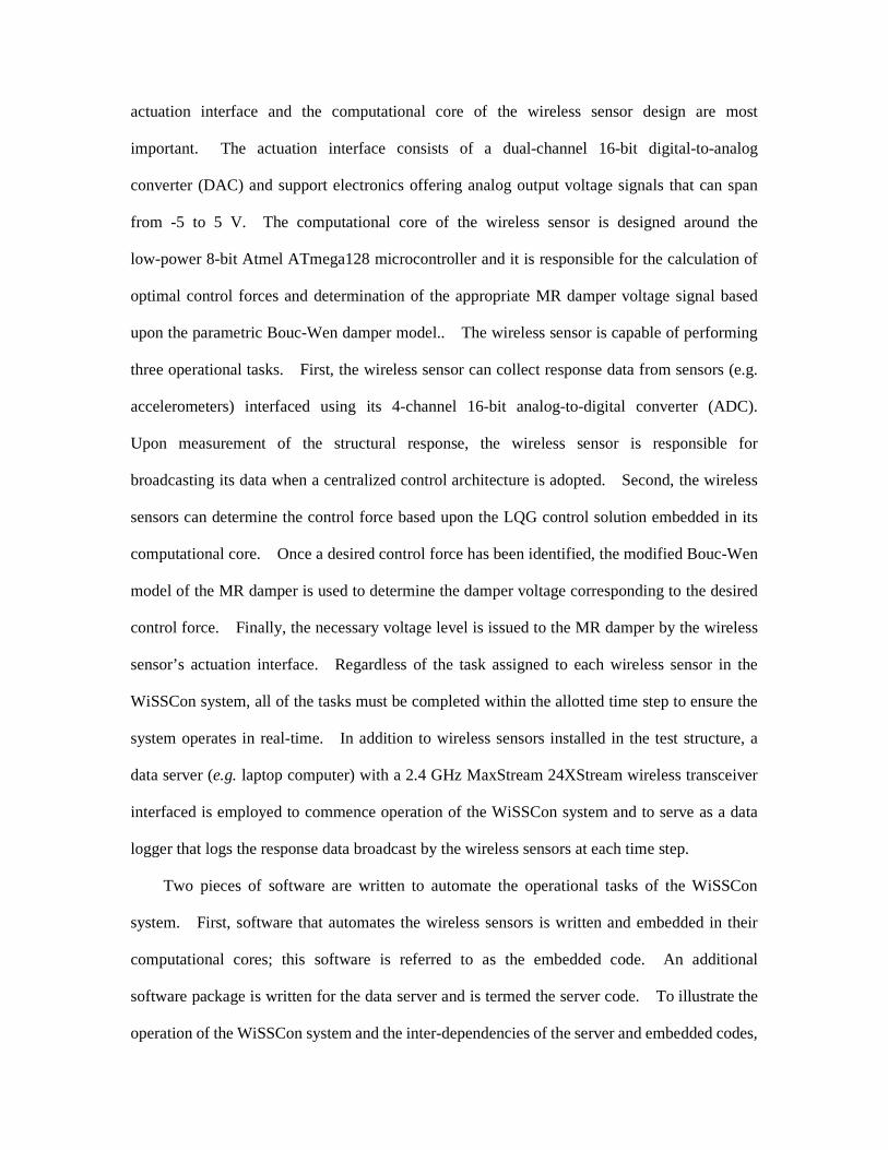
actuation interface and the computational core of the wireless sensor design are most

important. The actuation interface consists of a dual-channel 16-bit digital-to-analog

converter (DAC) and support electronics offering analog output voltage signals that can span

from -5 to 5 V. The computational core of the wireless sensor is designed around the

low-power 8-bit Atmel ATmega128 microcontroller and it is responsible for the calculation of

optimal control forces and determination of the appropriate MR damper voltage signal based

upon the parametric Bouc-Wen damper model.. The wireless sensor is capable of performing

three operational tasks. First, the wireless sensor can collect response data from sensors (e.g.

accelerometers) interfaced using its 4-channel 16-bit analog-to-digital converter (ADC).

Upon measurement of the structural response, the wireless sensor is responsible for

broadcasting its data when a centralized control architecture is adopted. Second, the wireless

sensors can determine the control force based upon the LQG control solution embedded in its

computational core. Once a desired control force has been identified, the modified Bouc-Wen

model of the MR damper is used to determine the damper voltage corresponding to the desired

control force. Finally, the necessary voltage level is issued to the MR damper by the wireless

sensor’s actuation interface. Regardless of the task assigned to each wireless sensor in the

WiSSCon system, all of the tasks must be completed within the allotted time step to ensure the

system operates in real-time. In addition to wireless sensors installed in the test structure, a

data server (e.g. laptop computer) with a 2.4 GHz MaxStream 24XStream wireless transceiver

interfaced is employed to commence operation of the WiSSCon system and to serve as a data

logger that logs the response data broadcast by the wireless sensors at each time step.

Two pieces of software are written to automate the operational tasks of the WiSSCon

system. First, software that automates the wireless sensors is written and embedded in their

computational cores; this software is referred to as the embedded code. An additional

software package is written for the data server and is termed the server code. To illustrate the

operation of the WiSSCon system and the inter-dependencies of the server and embedded codes,

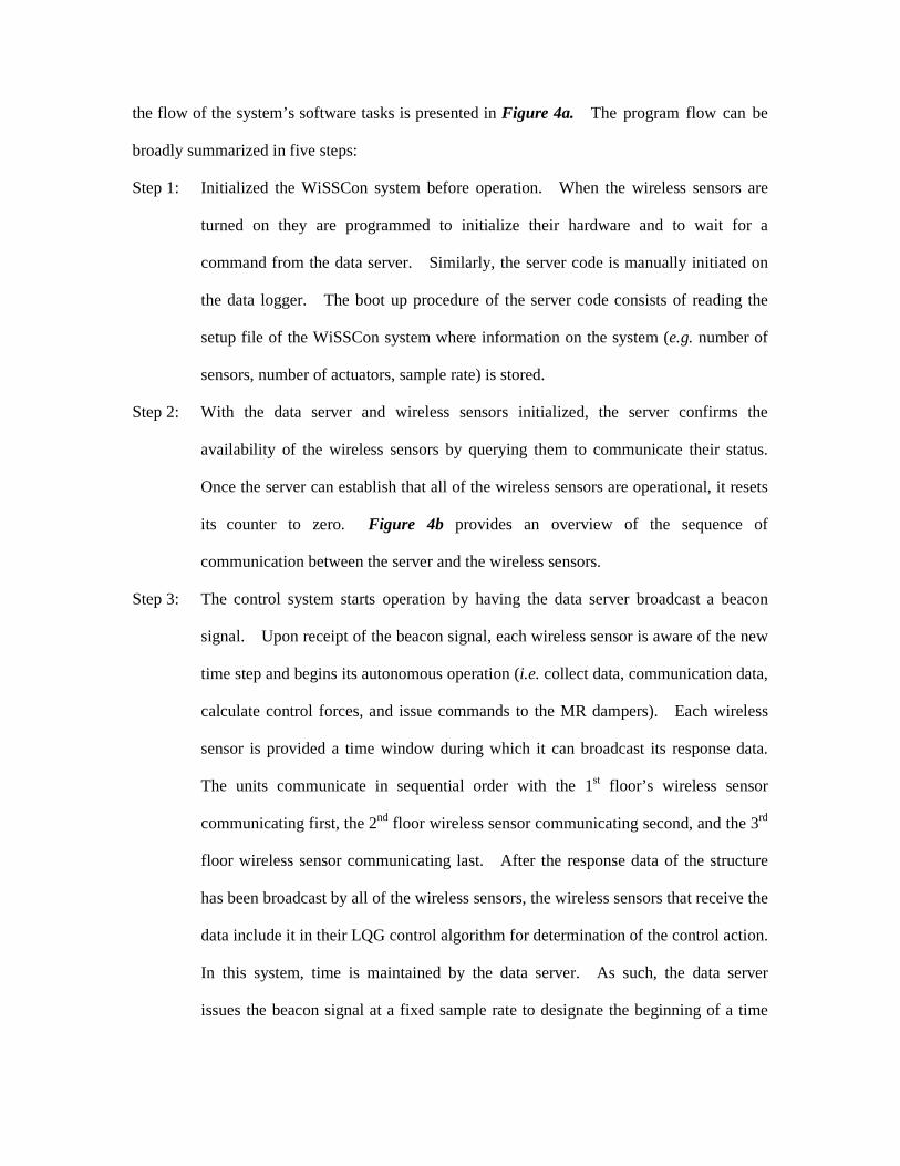
the flow of the system’s software tasks is presented in Figure 4a. The program flow can be

broadly summarized in five steps:

Step 1: Initialized the WiSSCon system before operation. When the wireless sensors are

turned on they are programmed to initialize their hardware and to wait for a

command from the data server. Similarly, the server code is manually initiated on

the data logger. The boot up procedure of the server code consists of reading the

setup file of the WiSSCon system where information on the system (e.g. number of

sensors, number of actuators, sample rate) is stored.

Step 2: With the data server and wireless sensors initialized, the server confirms the

availability of the wireless sensors by querying them to communicate their status.

Once the server can establish that all of the wireless sensors are operational, it resets

its counter to zero. Figure 4b provides an overview of the sequence of

communication between the server and the wireless sensors.

Step 3: The control system starts operation by having the data server broadcast a beacon

signal. Upon receipt of the beacon signal, each wireless sensor is aware of the new

time step and begins its autonomous operation (i.e. collect data, communication data,

calculate control forces, and issue commands to the MR dampers). Each wireless

sensor is provided a time window during which it can broadcast its response data.

The units communicate in sequential order with the 1st floor’s wireless sensor

communicating first, the 2nd floor wireless sensor communicating second, and the 3rd

floor wireless sensor communicating last. After the response data of the structure

has been broadcast by all of the wireless sensors, the wireless sensors that receive the

data include it in their LQG control algorithm for determination of the control action.

In this system, time is maintained by the data server. As such, the data server

issues the beacon signal at a fixed sample rate to designate the beginning of a time

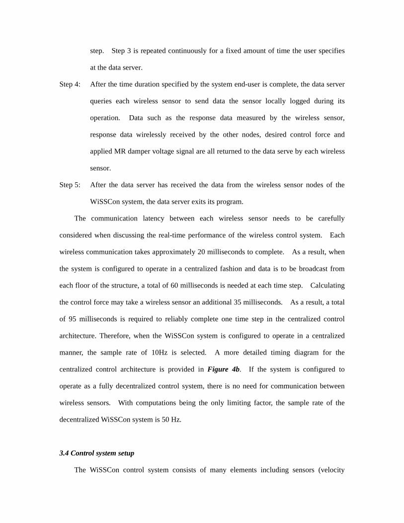
step. Step 3 is repeated continuously for a fixed amount of time the user specifies

at the data server.

Step 4: After the time duration specified by the system end-user is complete, the data server

queries each wireless sensor to send data the sensor locally logged during its

operation. Data such as the response data measured by the wireless sensor,

response data wirelessly received by the other nodes, desired control force and

applied MR damper voltage signal are all returned to the data serve by each wireless

sensor.

Step 5: After the data server has received the data from the wireless sensor nodes of the

WiSSCon system, the data server exits its program.

The communication latency between each wireless sensor needs to be carefully

considered when discussing the real-time performance of the wireless control system. Each

wireless communication takes approximately 20 milliseconds to complete. As a result, when

the system is configured to operate in a centralized fashion and data is to be broadcast from

each floor of the structure, a total of 60 milliseconds is needed at each time step. Calculating

the control force may take a wireless sensor an additional 35 milliseconds. As a result, a total

of 95 milliseconds is required to reliably complete one time step in the centralized control

architecture. Therefore, when the WiSSCon system is configured to operate in a centralized

manner, the sample rate of 10Hz is selected. A more detailed timing diagram for the

centralized control architecture is provided in Figure 4b. If the system is configured to

operate as a fully decentralized control system, there is no need for communication between

wireless sensors. With computations being the only limiting factor, the sample rate of the

decentralized WiSSCon system is 50 Hz.

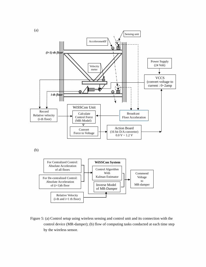
3.4 Control system setup

The WiSSCon control system consists of many elements including sensors (velocity

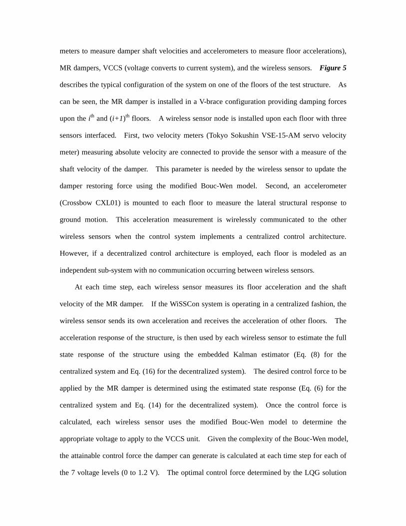
meters to measure damper shaft velocities and accelerometers to measure floor accelerations),

MR dampers, VCCS (voltage converts to current system), and the wireless sensors. Figure 5

describes the typical configuration of the system on one of the floors of the test structure. As

can be seen, the MR damper is installed in a V-brace configuration providing damping forces

upon the ith and (i+1)th floors. A wireless sensor node is installed upon each floor with three

sensors interfaced. First, two velocity meters (Tokyo Sokushin VSE-15-AM servo velocity

meter) measuring absolute velocity are connected to provide the sensor with a measure of the

shaft velocity of the damper. This parameter is needed by the wireless sensor to update the

damper restoring force using the modified Bouc-Wen model. Second, an accelerometer

(Crossbow CXL01) is mounted to each floor to measure the lateral structural response to

ground motion. This acceleration measurement is wirelessly communicated to the other

wireless sensors when the control system implements a centralized control architecture.

However, if a decentralized control architecture is employed, each floor is modeled as an

independent sub-system with no communication occurring between wireless sensors.

At each time step, each wireless sensor measures its floor acceleration and the shaft

velocity of the MR damper. If the WiSSCon system is operating in a centralized fashion, the

wireless sensor sends its own acceleration and receives the acceleration of other floors. The

acceleration response of the structure, is then used by each wireless sensor to estimate the full

state response of the structure using the embedded Kalman estimator (Eq. (8) for the

centralized system and Eq. (16) for the decentralized system). The desired control force to be

applied by the MR damper is determined using the estimated state response (Eq. (6) for the

centralized system and Eq. (14) for the decentralized system). Once the control force is

calculated, each wireless sensor uses the modified Bouc-Wen model to determine the

appropriate voltage to apply to the VCCS unit. Given the complexity of the Bouc-Wen model,

the attainable control force the damper can generate is calculated at each time step for each of

the 7 voltage levels (0 to 1.2 V). The optimal control force determined by the LQG solution

is then compared to this list of attainable control forces; the wireless sensor selects the voltage

level offering the control force closest to that desired by the LQG controller. To ensure the

Bouc-Wen model is updated for the next time step, the wireless sensor updates the restoring

force of the model using Eq. (15). Figure 5b provides a flow chart of the flow of calculations

made by each wireless sensor during the operation of the WiSSCon system.

4. DISCUSSIONS OF THE EXPERIMENTAL RESULTS

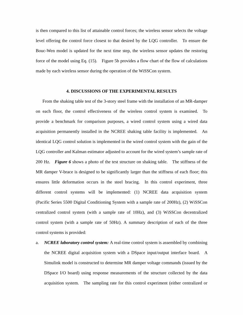
From the shaking table test of the 3-story steel frame with the installation of an MR-damper

on each floor, the control effectiveness of the wireless control system is examined. To

provide a benchmark for comparison purposes, a wired control system using a wired data

acquisition permanently installed in the NCREE shaking table facility is implemented. An

identical LQG control solution is implemented in the wired control system with the gain of the

LQG controller and Kalman estimator adjusted to account for the wired system’s sample rate of

200 Hz. Figure 6 shows a photo of the test structure on shaking table. The stiffness of the

MR damper V-brace is designed to be significantly larger than the stiffness of each floor; this

ensures little deformation occurs in the steel bracing. In this control experiment, three

different control systems will be implemented: (1) NCREE data acquisition system

(Pacific Series 5500 Digital Conditioning System with a sample rate of 200Hz), (2) WiSSCon

centralized control system (with a sample rate of 10Hz), and (3) WiSSCon decentralized

control system (with a sample rate of 50Hz). A summary description of each of the three

control systems is provided:

a. NCREE laboratory control system: A real-time control system is assembled by combining

the NCREE digital acquisition system with a DSpace input/output interface board. A

Simulink model is constructed to determine MR damper voltage commands (issued by the

DSpace I/O board) using response measurements of the structure collected by the data

acquisition system. The sampling rate for this control experiment (either centralized or

decentralized control) is 200Hz and the LQG control algorithm will be used. The result

from this control system will be used for comparison with the wireless control system

(centralized and decentralized).

b. Centralized wireless control with a sampling rate of 10 Hz: In the centralized architectural

configuration of the WiSSCon system, the wireless sensors on each floor will measure their

respective acceleration and broadcast that measurement to the other wireless sensors

situated on different floors. If a high sample rate is chosen, then there is a chance data

could be lost due to dropped packets or packet collisions in the wireless channel. To

ensure data loss kept below 2%, a sample rate of 10 Hz is used [Lynch et al., 2006b].

c. Decentralized wireless control with a sample rate of 50 Hz: In the decentralized control

system, each wireless sensor only receives measurement data from the sensors on its own

floor. Since there is no need to wait for the wireless transmission of data, the sample rate

can be higher; a rate of 50Hz is employed.

4.1 Validation of the WiSSCon system

In order to verify the measurement accuracy of the wireless control system (centralized and

decentralized) and the validity of the embedded algorithms (specifically, the modified

Bouc-Wen damper model), the wireless control system time-histories will be compared to that

redundantly recorded by the NCREE tethered data acquisition system. The El Centro (1940,

NS) ground motion record scaled to a peak acceleration of 200 gal is adopted during this study.

Although the table has 6 degrees-of-freedom, the ground motion is only applied in one lateral

direction.

a. First, the command voltage issued by the wireless sensors and that measured by the

laboratory data acquisition system show one-to-one agreement. As presented in Figure 7,

the command voltage calculated by the wireless sensor and applied to an MR damper

during the El Centro earthquake record is identical to that measured by the tethered data

acquisition system.

b. Next, the acceleration response of the structure as measured by each wireless sensor is

compared to the same acceleration response time-history wirelessly received by the other

wireless sensors during an excitation. This comparison is intended to identify any issues

associated with the communication of data in the wireless control system. As shown in

Figure 8, the acceleration time histories are wirelessly received without error and data loss

during excitation.

c. The accuracy of the LQG control solution embedded in the wireless sensor computational

core is validated by comparing the voltage output from the wireless sensor to that

theoretically calculated off-line using the response data recorded by the wireless sensor.

This is done for both the centralized and decentralized WiSSCon architectures. As shown

in Figure 9, there is good agreement between the command voltage generated by the

off-line numerical simulation and the experimentally obtained command voltage signal.

d. Similarly, the accuracy of the modified Bouc-Wen model in converting the LQG control

force into a command voltage to be applied to the MR damper is verified. Figures 10a

and 10c show the damper’s shaft velocity and the voltage signal generated by the wireless

sensor’s Bouc-Wen model during the application of the El Centro ground motion record.

As can be seen in Figure 10b, the damper force measured by the laboratory data

acquisition system from a load cell installed on the 1st floor MR damper (dash line) is in

strong agreement with the LQG control force calculated by the wireless sensor (solid line).

From the above mentioned validation tests, the WiSSCon system has proven that it can reliably

command the correct voltage to attain a desired control force, that there is no loss of data

during communication, and that the actuation interface is capable of generating the correct

control voltage.

4.2 Validation of wireless control effectiveness

An evaluation of MR-damper performance during experimentation is important in

assessing the effectiveness of the control system. During the application of the centralized

control system to the test structure, the hysteretic behavior of each MR damper is examined.

First, the centralized WiSSCon system is used to control the test structure; during a second

round of testing, the NCREE control system is used implementing the same Bouc-Wen and

LQG algorithms at 10 Hz. Alternatively, the wired NCREE control system is also operated at

200 Hz to see if the higher sample rate impacts the hysteretic properties of the damper.

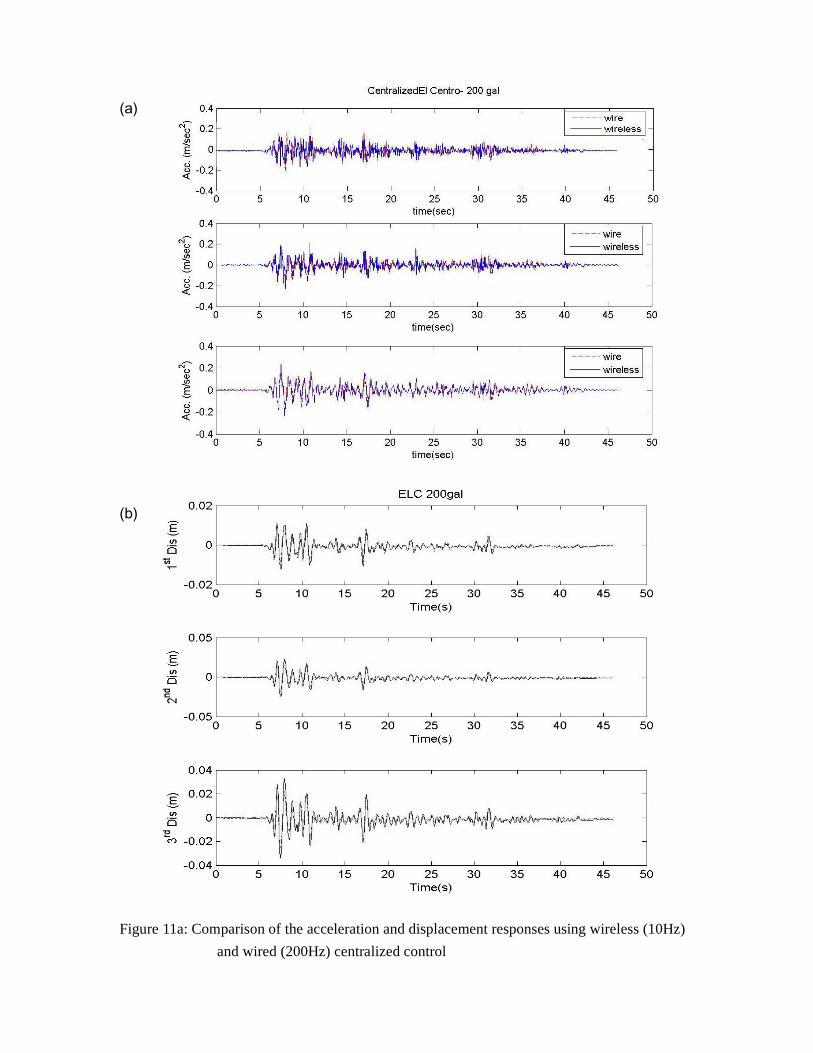
To verify the ability of the wireless control system to mitigate the dynamic response of the

test structure, response time histories (acceleration and displacement) of the test structure are

compared between those obtained using the wireless and wired control systems. Comparison

on the floor acceleration and displacement using the wired control system (200Hz) and the

wireless control system (10Hz) for a centralized control architecture is presented in Figure 11a,

and comparison on the floor acceleration and displacement using wireless control system

between the case of centralized control (10Hz) and the decentralized control (50 Hz) is shown

in Figure 11b. The strong agreement in the mitigated time histories reveals the effectiveness

of the WiSSCon system in controlling the test structure; in general, the performance of the

wireless control system is on par with that of the tethered laboratory control system.

A comparison between the closed-loop feedback control and passive mitigation methods

is also made. For cases of passive-on (constant 1.2 V supplied to the MR-damper to attain the

maximum damping coefficient), passive-off (constant 0V supplied to the MR-damper to attain

the minimum damping coefficient), wireless 10Hz centralized control, wireless 50 Hz

decentralized control, wired 200Hz centralized control and wired 200Hz decentralized control,

peak structural responses are recorded and compared. The results of the comparative study

are presented in Figure 12. It is concluded that both centralized and decentralized control

using the wireless sensing system can reach almost the same control effectiveness as the wired

control system. Furthermore, the closed-loop feedback control results generally outperform

those of the passive-on and passive-off cases.

5. CONCLUSIONS

This study examines the potential use of wireless communication and embedded computing

technologies within real-time structural control applications. Based on the implementation of

the prototype WiSSCon system in a three story steel test structure, both the centralized and

decentralized control architectures are implemented to mitigate the lateral response of the test

structure using MR dampers. During the test, a large earthquake time history is applied (El

Centro (1940 NS) scaled to a peak acceleration of 200 gal) at the structure base using a shaking

table. Three major performance attributes of the wireless control system were examined: (1)

validation of the reliability of wireless communications for real-time applications, (2)

validation of a modified Bouc-Wen damper model embedded in the wireless sensors to operate

the MR dampers, and (3) exploration between the control effectiveness when using WiSSCon

in a centralized and decentralized architectural configuration. The following conclusions

have been drawn:

1. In this study, the WiSSCon system for structural control has been demonstrated. The

performance of this novel control technology has been shown to be nearly comparable to

that of the wired control system. Issues of stability have not been considered because of

the inherent bounded input/bounded output (BIBO) nature of the semi-active control

approach.

2. When applying wireless sensor networks to real-time applications, communication latency

must be carefully examined. In this study, reliability of the wireless communication

channel is attained by slowing the system down. Alternatively, if a sample rate greater

than 10 Hz is desired, decentralization offers one potential solution (with an attainable

sample rate of 50 Hz). In the decentralized control system, only local sensor information

is needed to generate the control signal sent to the MR damper. As a result, such an

approach could be easily carried out for large-scale structural systems.

3. An advantage of the decentralized control approach is its robustness to failure. In other

words, the approach ensures that the control system can still operate should one damper

fail to operate properly. Given one subsystem fails, the other subsystems will be capable

of compensating accordingly and ensure suitable global performance of the system.

Finally, this study proves that wireless sensor networks are a promising technology capable

of operating in a real-time environment. The displacement and acceleration response of the

structure when using WiSSCon is nearly identical to that attained when using the wired

laboratory control system. While great success has been encountered in this study, further work

is needed to further refine wireless sensors for deployment in real civil structures using

structural control for response mitigation. Future efforts will be focused on modification of

the wireless sensor hardware to be able to attain higher sample rates consistent with the current

state-of-practice (50 Hz or greater). In addition, partially decentralized control architectures

remain an unexplored arena for potential use in a wireless structural control system.

ACKNOWLEDGEMENTS

This research has been supported by both the National Science Council, Taiwan, under grant

No. NSC 94-2625–Z -002-031 and No. NSC 95-2221-E-002-311. Additional support has been

provided to Prof. J. P. Lynch (University of Michigan) by the National Science Foundation

(Grant CMS-0528867) and the Office of Naval Research (Young Investigator Program). The

authors would also like to express their gratitude to NCREE technicians for their assistance

when conducting the shaking table experiments, and would also like to acknowledge the

support and guidance offered by Prof. Kincho Law during all phases of this research endeavor.

REFERENCES

Doyle, J. C., Glover, K., Khargonekar, P. P., and Francis, B. A., “State-space solutions to

standard H2 and H∞ control problems,” IEEE Transactions on Automatic Control, 34, 1989,

831-847.

Dyke, S.J., Spencer, B.F., Sain, M.K. and Carlson, J. D., “Modeling and control of

magnetorheological dampers for seismic response reduction,” Smart Materials and

Structures, 5, 1996, 565-575.

Dyke, S.J., Spencer, B.F., Quast, P. Sain, M.K., Kaspaari, D.C. and Soong, T.T., “Acceleration

feedback control of MDOF structures,” ASCE, J. of Engineering Mechanics, 122(9), 1996,

907-917.

Kurino, H., Tagami, J., Shimizu, K. And Kobori, T., “Switching oil damper with built-in

controller for structural control,” J. of Structural engineering, ASCE, Vol. 129, No.7, 2003,

895-904.

Lin, P.Y., P.N. Roschke, C. H. Loh and C. P. Cheng, “Semi-Active controlled based-isolation

system with MR dampers and pendulum system,”, 13WCEE, Vancouver, August, 2004,

paper #691.

Lin, P.Y., Roschke, P. and Loh, C. H, “System identification and real application of a smart

magneto-rheological damper,” Proceedings of the 2005 IEEE International Symposium

on Intelligent Control, Limassol, Cyprus, 2005, 989-994.

Lin, P.Y., Chung, L.L., Loh, C.H., Cheng, C.P., Roschke, P.N. and Chang, C.C., “Experimental

study of seismic protection for structures using MR dampers,” Proceedings of the 12th

European Conference on Earthquake Engineering, London, September, 2002, paper #249.

Lynch, J. P., Sundararajan, A., Law, K. H., Kiremidjian, A. S., and Carryer, E., “Embedded

damage detection algorithms in a Wireless Sensing Unit for Attainment of Operational

Power efficiency,” Smart Materials and Structures, IOP, Vol.13, No.4, 2004, 800-810.

Lynch, J. P., Loh, K. J., Hou, T. C., Wang, Y., Yi, J., Yun, C. B., Lu, K. and Loh, C. H. "

Validation case studies of wireless monitoring systems in civil structures," Proceedings of

the 2nd International Conference on Structural Health Monitoring of Intelligent

Infrastructure (SHMII-2) , Shenzhen, China, November, 2005, 597-604.

Lynch, J. P., Wang, Y., Lu, K. C., Hou, T. C., and Loh, C. H., “Post-seismic Damage

Assessment of Steel Structures Instrumented with Self-interrogating wireless Sensors,”

Proceedings of the 8th National Conference on Earthquake Engineering, San Francisco, CA,

USA, April 18-22, 2006a.

Lynch, J. P., Wang, Y., Swartz, R. A., Lu, K. C. and Loh, C. H., “Implementation of a

closed-loop structural control system using wireless sensor networks,” submit to J. of

Structural Control and Health Monitoring (2006b).

Nishitani, A., Nitta, Y. and Ikeda, Y., “Semiactive structural-control based on variable

slip-force level dampers,” J. of Structural Engineering, ASCE, Vol.129, No.7, 2003,

933-940.

Spencer, B.F., Dyke, S.J., Sain, M.K. and Carlson, J. D., “Phenomenological model for

magnetorheological dampers,” J. Engineering Mechanics, ASCE, 123, 1997, 230-238.

Spencer, B. F. and Nagarajaiah, S., “State of the art of structural control,” J. Structural

Engineering, ASCE, 129, 2003, 845-856.

Straser, E. G. and Kiremidjian, A. S., “A modular, wireless damage monitoring system for

structures,” Report No.129, John A. Blume Earthquake Engineering Research Center,

Department of Civil & Environmental Engineering, Stanford University, CA 1998.

Wang, Y., Lynch, L. P., Law, K. H., “Design of a low-power wireless structural monitoring

system for collaborative computational algorithms,” Proceedings of SPIE 10th annual Int.

Symposium on Nondestructive Evaluation for Health Monitoring and Diagnostics, San

Diego, CA, March 6-10, 2005.

Yang, G., Spencer, B.F., Carlson, J. D. and Sain, M.K., “Large-scale MR fluid dampers:

modeling and dynamic performance consideration,” Engineering Structures, 24, 2002,

309-323.

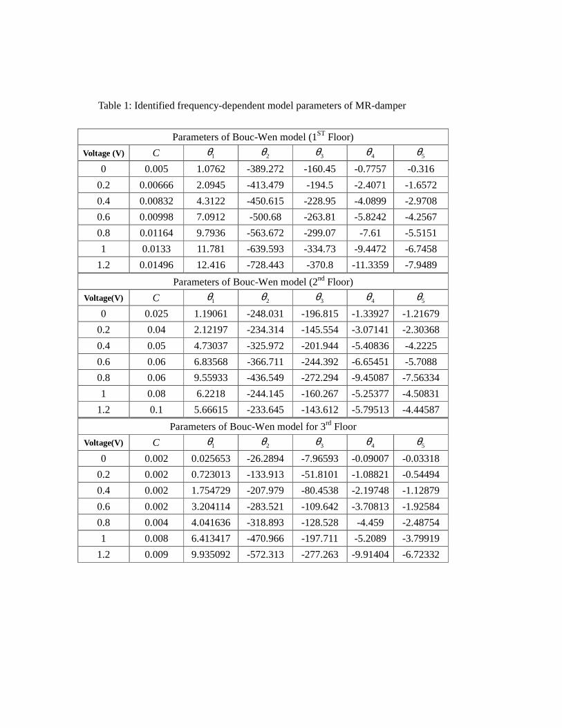
Table 1: Identified frequency-dependent model parameters of MR-damper

Parameters of Bouc-Wen model (1ST Floor)

Voltage (V) C 1θ 2θ 3θ 4θ 5θ

0 0.005 1.0762 -389.272 -160.45 -0.7757 -0.316

0.2 0.00666 2.0945 -413.479 -194.5 -2.4071 -1.6572

0.4 0.00832 4.3122 -450.615 -228.95 -4.0899 -2.9708

0.6 0.00998 7.0912 -500.68 -263.81 -5.8242 -4.2567

0.8 0.01164 9.7936 -563.672 -299.07 -7.61 -5.5151

1 0.0133 11.781 -639.593 -334.73 -9.4472 -6.7458

1.2 0.01496 12.416 -728.443 -370.8 -11.3359 -7.9489

Parameters of Bouc-Wen model (2nd Floor)

Voltage(V) C 1θ 2θ 3θ 4θ 5θ

0 0.025 1.19061 -248.031 -196.815 -1.33927 -1.21679

0.2 0.04 2.12197 -234.314 -145.554 -3.07141 -2.30368

0.4 0.05 4.73037 -325.972 -201.944 -5.40836 -4.2225

0.6 0.06 6.83568 -366.711 -244.392 -6.65451 -5.7088

0.8 0.06 9.55933 -436.549 -272.294 -9.45087 -7.56334

1 0.08 6.2218 -244.145 -160.267 -5.25377 -4.50831

1.2 0.1 5.66615 -233.645 -143.612 -5.79513 -4.44587

Parameters of Bouc-Wen model for 3rd Floor

Voltage(V) C 1θ 2θ 3θ 4θ 5θ

0 0.002 0.025653 -26.2894 -7.96593 -0.09007 -0.03318

0.2 0.002 0.723013 -133.913 -51.8101 -1.08821 -0.54494

0.4 0.002 1.754729 -207.979 -80.4538 -2.19748 -1.12879

0.6 0.002 3.204114 -283.521 -109.642 -3.70813 -1.92584

0.8 0.004 4.041636 -318.893 -128.528 -4.459 -2.48754

1 0.008 6.413417 -470.966 -197.711 -5.2089 -3.79919

1.2 0.009 9.935092 -572.313 -277.263 -9.91404 -6.72332

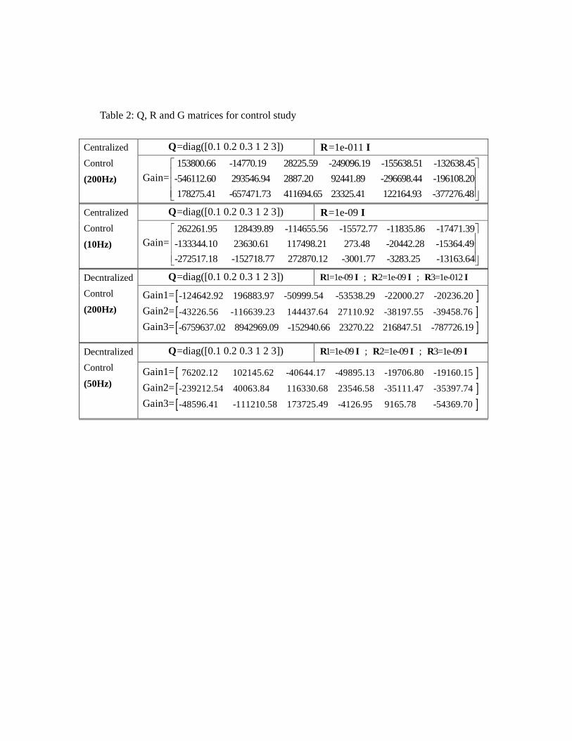
Table 2: Q, R and G matrices for control study

=diag([0.1 0.2 0.3 1 2 3])Q =1e-011 R I Centralized

Control

(200Hz) Gain= 153800.66 -14770.19 28225.59 -249096.19 -155638.51 -132638.45

-546112.60 293546.94 2887.20 92441.89 -296698.44 -196108.20

178275.41 -657471.73 411694.65 23325.41 122164.93 -377276.48

=diag([0.1 0.2 0.3 1 2 3])Q =1e-09 R I Centralized

Control

(10Hz) Gain= 262261.95 128439.89 -114655.56 -15572.77 -11835.86 -17471.39

-133344.10 23630.61 117498.21 273.48 -20442.28 -15364.49

-272517.18 -152718.77 272870.12 -3001.77 -3283.25 -13163.64

=diag([0.1 0.2 0.3 1 2 3])Q 1=1e-09 ; 2=1e-09 ; 3=1e-012 R I R I R I Decntralized

Control

(200Hz)

Gain1=[ ]-124642.92 196883.97 -50999.54 -53538.29 -22000.27 -20236.20

Gain2=[ ]-43226.56 -116639.23 144437.64 27110.92 -38197.55 -39458.76

Gain3=[ ]-6759637.02 8942969.09 -152940.66 23270.22 216847.51 -787726.19

=diag([0.1 0.2 0.3 1 2 3])Q 1=1e-09 ; 2=1e-09 ; 3=1e-09 R I R I R I Decntralized

Control

(50Hz) Gain1=[ ] 76202.12 102145.62 -40644.17 -49895.13 -19706.80 -19160.15

Gain2=[ ]-239212.54 40063.84 116330.68 23546.58 -35111.47 -35397.74

Gain3=[ ]-48596.41 -111210.58 173725.49 -4126.95 9165.78 -54369.70

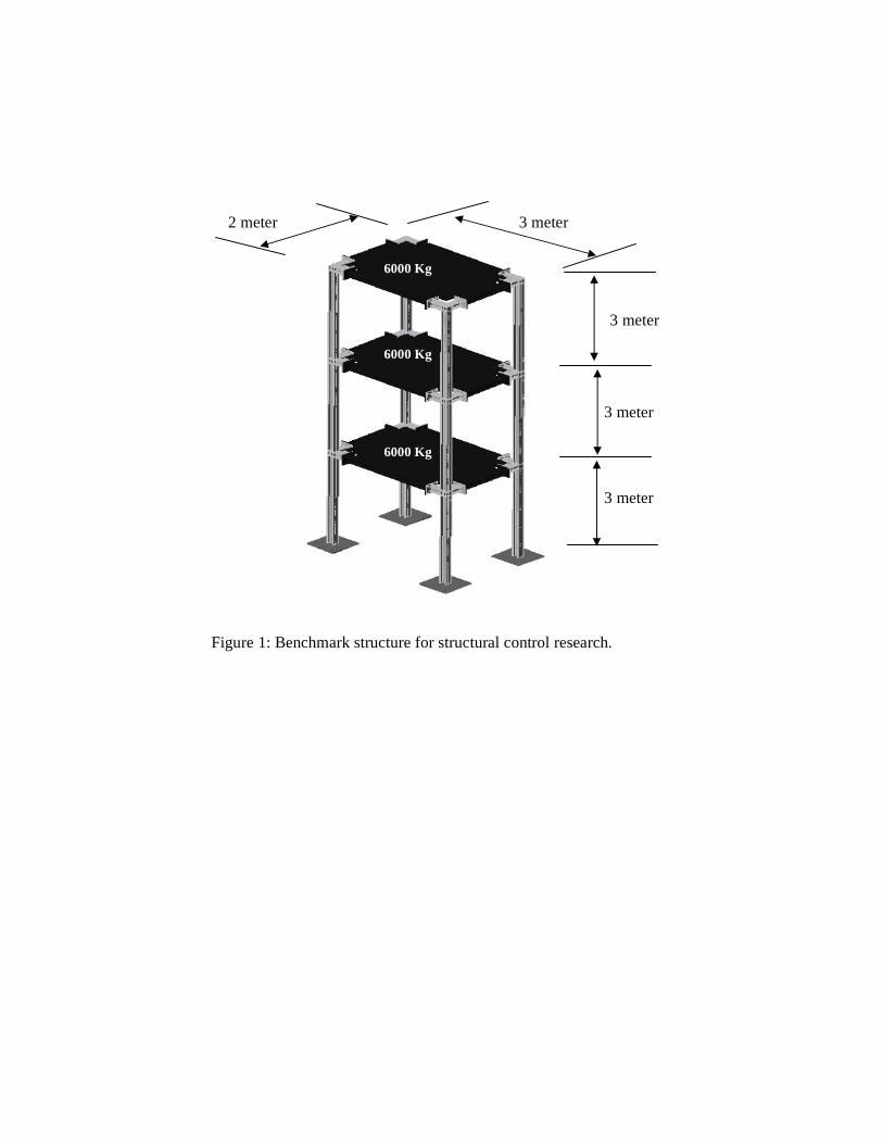
Figure 1: Benchmark structure for structural control research.

3 meter 2 meter

3 meter

3 meter

3 meter

6000 Kg

6000 Kg

6000 Kg

(a) (b)

Figure 2: Comparison between the measured data and the simulation result on

(a) Force versus displacement relationship,

(b) Force versus velocity relationship,

from random stroke random voltage test of MR-damper.

-0.02 -0.01 0 0.01 0.02-0.02

-0.015

-0.01

-0.005

0

0.005

0.01

0.015

0.02

Displacement (m)

Dam

per

forc

e (

MN

)

measured

simulated

-0.2 -0.1 0 0.1 0.2 0.3-0.02

-0.015

-0.01

-0.005

0

0.005

0.01

0.015

0.02

Velocity (m/s)

Dam

per

forc

e (M

N)

measured

simulated

(a)

(b)

Figure 3: Architecture of wireless control unit; (a) hardware architectural design; (b)

picture of wireless sensor prototype prior to installation in the test structure

[Lynch et al., 2006b]

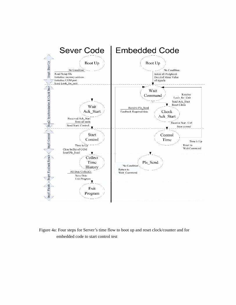
Figure 4a: Four steps for Server’s time flow to boot up and reset clock/counter and for

embedded code to start control test

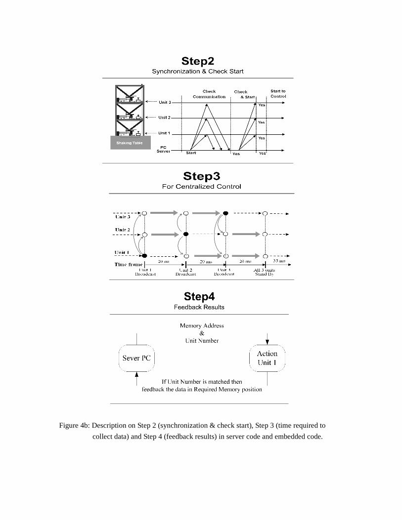
Figure 4b: Description on Step 2 (synchronization & check start), Step 3 (time required to

collect data) and Step 4 (feedback results) in server code and embedded code.

(a)

(b)

Relative Velocity (i-th and i+1 th floor)

WiSSCon System

Control Algorithm With

Kalman Estimator

Inverse Model of MR-Damper

For De-centralized Control: Absolute Acceleration

of (i+1)th floor

Commend Voltage

to MR-damper

For Centralized Control: Absolute Acceleration

of all floors

Figure 5: (a) Control setup using wireless sensing and control unit and its connection with the

control device (MR-damper); (b) flow of computing tasks conducted at each time step

by the wireless sensor.

Record Relative velocity

(i-th floor)

Broadcast Floor Acceleration

WiSSCon Unit

Calculate Control Force (MR-Model)

Convert Force to Voltage

Action Board (16 bit D/A converter)

0.0 V ~ 1.2 V

VCCS (convert voltage to current : 0~2amp

Amp)

Power Supply (24 Volt)

Sensing unit

Accelerometer

Velocity meter

i-th floor

(i+1)-th floor

Figure 6: (a) Photo of the 3-story test structure on NCREE shaking table;

(b) Photo of the MR-damper on the first floor.

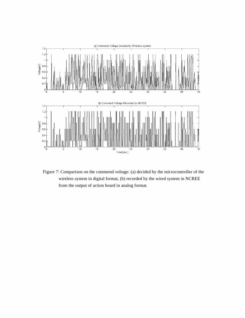
Figure 7: Comparison on the commend voltage: (a) decided by the microcontroller of the

wireless system in digital format, (b) recorded by the wired system in NCREE

from the output of action board in analog format.

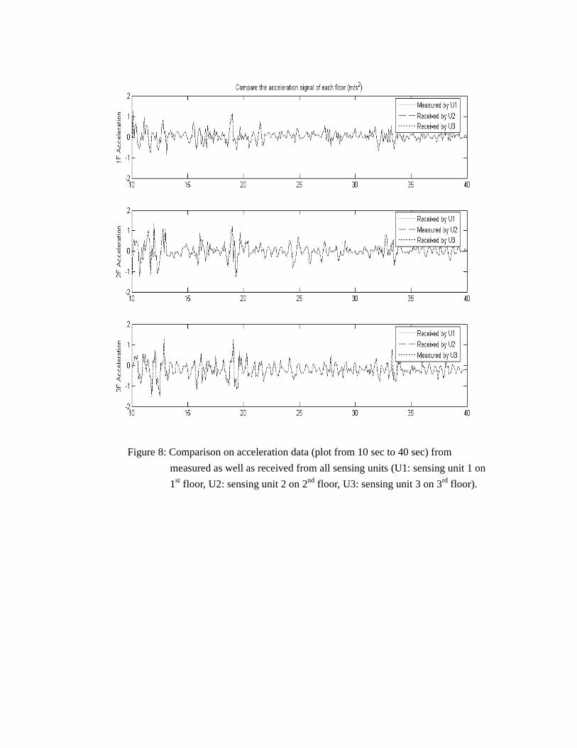
Figure 8: Comparison on acceleration data (plot from 10 sec to 40 sec) from

measured as well as received from all sensing units (U1: sensing unit 1 on

1st floor, U2: sensing unit 2 on 2nd floor, U3: sensing unit 3 on 3rd floor).

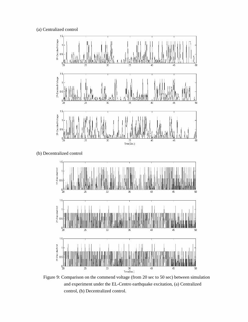
(a) Centralized control

(b) Decentralized control

Figure 9: Comparison on the commend voltage (from 20 sec to 50 sec) between simulation

and experiment under the EL-Centro earthquake excitation, (a) Centralized

control, (b) Decentralized control.

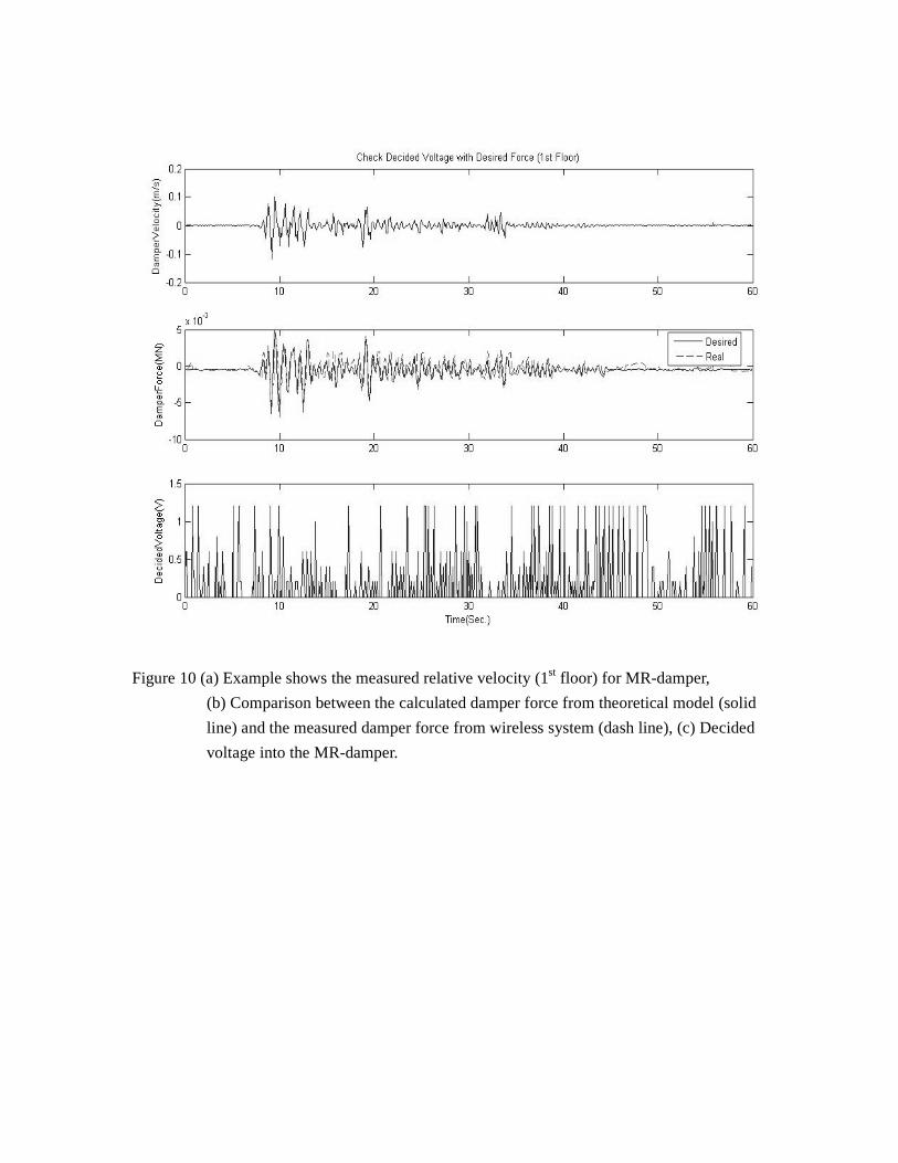
Figure 10 (a) Example shows the measured relative velocity (1st floor) for MR-damper,

(b) Comparison between the calculated damper force from theoretical model (solid

line) and the measured damper force from wireless system (dash line), (c) Decided

voltage into the MR-damper.

(a)

(b)

Figure 11a: Comparison of the acceleration and displacement responses using wireless (10Hz)

and wired (200Hz) centralized control

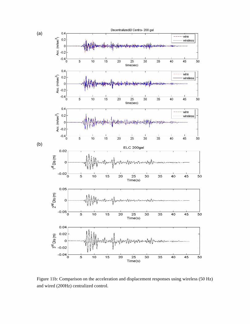
(a)

(b)

Figure 11b: Comparison on the acceleration and displacement responses using wireless (50 Hz)

and wired (200Hz) centralized control.

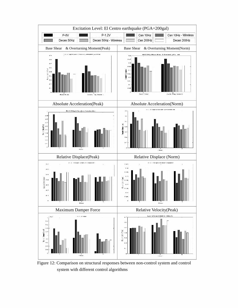
Excitation Level: El Centro earthquake (PGA=200gal)

Base Shear & Overturning Moment(Peak) Base Shear & Overturning Moment(Norm)

Absolute Acceleration(Peak) Absolute Acceleration(Norm)

Relative Displace(Peak) Relative Displace (Norm)

Maximum Damper Force Relative Velocity(Peak)

Figure 12: Comparison on structural responses between non-control system and control

system with different control algorithms