EXPERIMENTAL VALIDATION OF NON-COHESIVE SOIL USING

EXPERIMENTAL VALIDATION OF NON-COHESIVE SOIL USING DISCRETE

ELEMENT METHOD

A Thesis

Submitted to the Faculty

of

Purdue University

by

Ayan Roy

In Partial Fulfillment of the

Requirements for the Degree

of

Master of Science in Mechanical Engineering

December 2018

Purdue University

Indianapolis, Indiana

ii

THE PURDUE UNIVERSITY GRADUATE SCHOOL

STATEMENT OF COMMITTEE APPROVAL

Dr. Tamer Wasfy

Department of Mechanical and Energy Engineering

Dr. Andres Tovar


Dr. Hanzim El-Mounayri


Approved by:

Dr. Sohel Anwar

Chair of the Graduate Program

iii

ACKNOWLEDGMENTS

This thesis could not have been achievable without the assistance and support of

several individuals who in one way or another contributed their valuable help in the

preparation and completion of this study.

First of all, I would like to express my special thanks to Dr. Tamer Wasfy for

providing this opportunity for me to learn and gain this much experience throughout

my study. Without his technical advice and constant support, this work could not be

done.

Also, I want to thank my advising committee, Dr. Hazim El-Mounayri and Dr.

Andres Tovar for their time and direction during the completion of this thesis.

I also appreciate Mechanical Engineering Department faculty for their instruction

and advice through my graduate courses.

I would also like to extend my gratefulness to Valerie Lim Diemer for her kindness

in formatting this thesis and assisting me during my graduate studies.

I would like to thank my dear parents and sister for supporting and motivating

me through all the stages of my life. I am very proud to have such a nice and warm

family.

iv

TABLE OF CONTENTS

Page

LIST OF TABLES . . . . . . . . . . . . . . . . . . . . . . . . . . . . . . . . vi

LIST OF FIGURES . . . . . . . . . . . . . . . . . . . . . . . . . . . . . . . vii

ABSTRACT . . . . . . . . . . . . . . . . . . . . . . . . . . . . . . . . . . . x

1 INTRODUCTION . . . . . . . . . . . . . . . . . . . . . . . . . . . . . . 1

1.1 Motivation . . . . . . . . . . . . . . . . . . . . . . . . . . . . . . . . 1

1.2 Literature Review . . . . . . . . . . . . . . . . . . . . . . . . . . . . 2

1.2.1 Empirical Methods . . . . . . . . . . . . . . . . . . . . . . . 2

1.2.2 Lumped Parameters Parametric Analysis Methods . . . . . . 3

1.2.3 Computational Methods . . . . . . . . . . . . . . . . . . . . 6

1.3 Objectives and Contributions . . . . . . . . . . . . . . . . . . . . . 9

1.4 Tools Used . . . . . . . . . . . . . . . . . . . . . . . . . . . . . . . . 11

1.5 Thesis Organization . . . . . . . . . . . . . . . . . . . . . . . . . . . 11

2 MULTIBODY DYNAMICS FORMULATION . . . . . . . . . . . . . . . 13

2.1 Equations of Motion . . . . . . . . . . . . . . . . . . . . . . . . . . 13

2.2 Contact Model . . . . . . . . . . . . . . . . . . . . . . . . . . . . . 15

2.2.1 Penalty Normal Contact Model . . . . . . . . . . . . . . . . 17

2.2.2 Asperity Friction Model . . . . . . . . . . . . . . . . . . . . 17

2.2.3 Inter-Particle Contact Search . . . . . . . . . . . . . . . . . 20

2.2.4 Contact Point Search . . . . . . . . . . . . . . . . . . . . . . 21

2.3 Joint Constraints . . . . . . . . . . . . . . . . . . . . . . . . . . . . 23

2.3.1 Revolute Joints . . . . . . . . . . . . . . . . . . . . . . . . . 24

2.3.2 Prismatic Joints . . . . . . . . . . . . . . . . . . . . . . . . . 24

2.4 Actuators . . . . . . . . . . . . . . . . . . . . . . . . . . . . . . . . 25

2.4.1 Linear Actuator . . . . . . . . . . . . . . . . . . . . . . . . . 25

v

Page

2.4.2 Rotational Actuator . . . . . . . . . . . . . . . . . . . . . . 25

2.5 Explicit Solution Procedure . . . . . . . . . . . . . . . . . . . . . . 26

3 DIRECT SHEAR TEST . . . . . . . . . . . . . . . . . . . . . . . . . . . 29

3.1 Experiment and Simulation . . . . . . . . . . . . . . . . . . . . . . 29

3.2 Results and Explanation: . . . . . . . . . . . . . . . . . . . . . . . . 31

4 PRESSURE-SINKAGE TEST . . . . . . . . . . . . . . . . . . . . . . . . 39

4.1 Experiment and Simulation . . . . . . . . . . . . . . . . . . . . . . 40

4.2 Results and Explanation . . . . . . . . . . . . . . . . . . . . . . . . 42

5 RIGID WHEEL-SOIL INTERACTION . . . . . . . . . . . . . . . . . . . 49

5.1 Experimental Setup . . . . . . . . . . . . . . . . . . . . . . . . . . . 51

5.2 Results and Explanation . . . . . . . . . . . . . . . . . . . . . . . . 54

6 APPLICATION: PREDICTION OF MOBILITY OF A HUMVEE VEHI-CLE ON SOFT SOIL . . . . . . . . . . . . . . . . . . . . . . . . . . . . . 59

7 CONCLUDING REMARKS AND FUTURE WORK . . . . . . . . . . . 63

REFERENCES . . . . . . . . . . . . . . . . . . . . . . . . . . . . . . . . . . 65

vi

LIST OF TABLES

Table Page

3.1 MBD model properties for direct shear stress simulation . . . . . . . . 31

3.2 Particle properties for direct shear stress simulation . . . . . . . . . . . 34

3.3 Maximum direct shear stress at different normal load . . . . . . . . . . 38

4.1 MBD model properties for pressure-sinkage penetroplate simulation . . 42

4.2 Particle properties for pressure-sinkage penetroplate simulation . . . . . 43

5.1 Particle properties for rigid wheel test simulation . . . . . . . . . . . . 54

5.2 MBD model properties . . . . . . . . . . . . . . . . . . . . . . . . . . . 54

5.3 Body speed at different slip . . . . . . . . . . . . . . . . . . . . . . . . 56

6.1 Particle properties for full vehicle simulation . . . . . . . . . . . . . . . 60

6.2 MBD model properties of the vehicle . . . . . . . . . . . . . . . . . . . 61

vii

LIST OF FIGURES

Figure Page

1.1 Mohr circle in terramechanics [1]. . . . . . . . . . . . . . . . . . . . . . 5

1.2 Particle-to-particle normal and tangential contact properties. [1] . . . . 8

1.3 Particle-to-surface Normal and Tangential contact properties. [1] . . . . 8

2.1 Location of a point on a rigid body with respect to the local body frame(XLP) and the global reference frame (XGP) [28]. . . . . . . . . . . . . 16

2.2 Contact surface and contact node [28] . . . . . . . . . . . . . . . . . . . 18

2.3 Asperity-based physical interpretation of friction [28] . . . . . . . . . . 19

2.4 Asperity spring friction model where Ft is the tangential friction force,Fn is the normal force, µk is the kinetic friction coefficient, and vrt is therelative tangential velocity between the two points of contact [28] . . . 19

2.5 Cartesian grid domain decomposition [30] . . . . . . . . . . . . . . . . 21

2.6 Particle of cubical shape modeled using superquadric with N = 3 (left)and N = 8 (right) [31] . . . . . . . . . . . . . . . . . . . . . . . . . . . 22

2.7 Particle of cubical shape modeled using 8 spheres [31] . . . . . . . . . . 23

2.8 Particle of cubical shape modeled using a polygonal surface [31]. . . . . 24

2.9 Prismatic joint in 2D . . . . . . . . . . . . . . . . . . . . . . . . . . . . 25

2.10 Linear actuator connecting two points [28] [32] . . . . . . . . . . . . . . 26

2.11 Rotational actuator connecting three points [28] [32] . . . . . . . . . . 26

3.1 Direct shear stress experimental setup [36] . . . . . . . . . . . . . . . . 30

3.2 MBD simulation model hierarchy . . . . . . . . . . . . . . . . . . . . . 31

3.3 Joints and actuators in the MBD model of direct shear stress test . . . 32

3.4 Snapshots of the direct shear stress test experiment . . . . . . . . . . . 32

3.5 DEM particle model inside IVRESS showing number of particles and par-ticle radius . . . . . . . . . . . . . . . . . . . . . . . . . . . . . . . . . 32

3.6 IVRESS snapshot showing particle-particle contact properties . . . . . 33

viii

Figure Page

3.7 Comparison between simulation and test results with normal load of 16kPa[36] . . . . . . . . . . . . . . . . . . . . . . . . . . . . . . . . . . . . . . 35



3.10 Maximum shear stress plot of all the three simulations with varying normalload . . . . . . . . . . . . . . . . . . . . . . . . . . . . . . . . . . . . . 38

4.1 Pressure sinkage penetroplate experimental setup [36] . . . . . . . . . . 41


4.3 Joints and actuators in the MBD model of penetroplate pressure sinkagetest . . . . . . . . . . . . . . . . . . . . . . . . . . . . . . . . . . . . . . 43

4.4 Snapshot of penetroplate pressure sinkage simulation . . . . . . . . . . 44



4.7 Experimental results showing pressure vs sinkage at different plate widths[37] . . . . . . . . . . . . . . . . . . . . . . . . . . . . . . . . . . . . . . 45

4.8 Simulation results showing pressure vs sinkage at different plate widths 46

4.9 Comparison between simulation results and experimental results poly-fitted at 3cm plate width . . . . . . . . . . . . . . . . . . . . . . . . . . 47



5.1 Sinkage of a wheel on soft soil . . . . . . . . . . . . . . . . . . . . . . . 50

5.2 Experimental setup of the wheel test experiment [37] . . . . . . . . . . 52

5.3 Snapshots of the wheel test simulation from two different angles . . . . 52




ix

Figure Page

5.7 Joints and actuators in the MBD model of wheel test . . . . . . . . . . 55

5.8 Comparison of wheel torque - slip % between different terramechanicsapproaches with bars showing error compared to the experimental results[10] . . . . . . . . . . . . . . . . . . . . . . . . . . . . . . . . . . . . . . 57

5.9 Comparison of drawbar force - slip % between different terramechanicsapproaches with bars showing error compared to the experimental results[10] . . . . . . . . . . . . . . . . . . . . . . . . . . . . . . . . . . . . . . 58

6.1 Humvee MBD simulation on soft soil [38] . . . . . . . . . . . . . . . . . 60

6.2 Humvee MBD model [38] . . . . . . . . . . . . . . . . . . . . . . . . . . 60

6.3 Polygon surface of the tire [38] . . . . . . . . . . . . . . . . . . . . . . . 61

6.4 Various suspension joints of the vehicle [38] . . . . . . . . . . . . . . . 61

6.5 MBD model of the entire vehicle chassis system [38] . . . . . . . . . . . 62

x

ABSTRACT

Roy, Ayan. M.S.M.E., Purdue University, December 2018. Experimental Validationof Non-cohesive Soil Using Discrete Element Method. Major Professor: TamerWasfy.

In this thesis, an explicit time integration code which integrates multibody dy-

namics (MBD) and the discrete element method (DEM) is validated using three

previously published steady-state physical experiments for non-cohesive sand-type

material, namely: shear-cell for measuring shear stress versus normal stress; penetro-

plate pressure-sinkage test; and wheel drawbar pull-torque-slip test. The test results

are used to calibrate the material properties of the DEM soft soil model and validate

the coupled MBD-DEM code. All three tests are important because each test mea-

sures specific mechanical characteristics of the soil under various loading conditions.

Shear strength of the soil as a function of normal load help to understand shearing

of the soil under a vehicle wheel contact patch causing loss of traction. Penetroplate

pressure-sinkage test is used to calibrate and validate friction and shear strength char-

acteristics of the soil. Finally the rigid wheel-soil interaction test is used to predict

drawbar pull force and wheel torque vs. slip percentage and normal stress for a rigid

wheel. Wheel-Soil interaction test is important because it plays the role of ultimate

validation of the soil model tuned in the previous two experiments and also shows

how the soil model behaves in vehicle mobility applications.

All the aforementioned tests were modeled in the multibody dynamics software

using rigid bodies and various joints and actuators. The sand-type material is mod-

eled using discrete cubical particles. A penalty technique is used to impose nor-

mal contact constraints (including particle-particle and particle-wall contact). An

asperity-based friction model is used to model friction. A Cartesian Eulerian grid

contact search algorithm is used to allow fast contact detection between particles.

xi

A recursive bounding box contact search algorithm enabled fast contact detection

between the particles and polygonal body surfaces (such as walls, penetrometer, and

wheel). The governing equations of motion are solved along with contact constraint

equations using a time-accurate explicit solution procedure. The results show very

good agreement between the simulation and the experimental measurements. The

model is then demonstrated in a full-scale application of high-speed off-road vehicle

mobility on the sand-type soil.

1

1. INTRODUCTION

1.1 Motivation

Off-road locomotion exists since the invention of wheels in 3500 B.C. Off-road

equipment and vehicles are widely used in the fields of aerospace, military operations,

construction, cross-country transportation, and agriculture. Thought there had been

significant growth in technology, development on off-road machineries has been limited

to empiricism and trial-error process. Until, the 20th century, development of off-road

vehicles did not catch the attention of many engineers and researchers. It is important

to predict terrain behavior with respect to soil properties in order to predict the

performance of off-road vehicles and equipment in their working environment, such

study is called ‘Terramechanics’.

Terramechanics can be divided into: terrain-vehicle mechanics; and terrain-implement

mechanics. Terrain-vehicle mechanics deals with tractive performance of a vehicle on

an unprepared terrain in order to design the desired following systems:

• Steering system of an off-road Vehicle.

• Suspension System of an off-road vehicle, specifically mitigation of excessive

vehicle dynamics.

• Vehicle elements interacting with the terrain directly like tires, wheels, and

tracks.

• Driveline and powertrain of an off-road vehicle.

• Vehicle elements to mitigate noise, vibration and harshness (NVH) characteris-

tics of an off-road Vehicle such as cabin, and seats.

2

Knowledge of terramechanics can guide the automotive engineers in the design

decision. Similarly, terrain-implement mechanics can be used to design machinery

operating on unprepared terrain.

Analysis of systems with knowledge terramechanics will play a significant role in

the development of off-road vehicles and equipment. Therefore, research on soil and

predicting soil behavior with respect to its interaction with wheels using multibody

techniques and DEM approach will play a key role to develop a methodology to

accurately predict ‘Mobility and Maneuverability of Vehicles on Soft Soil.’

1.2 Literature Review

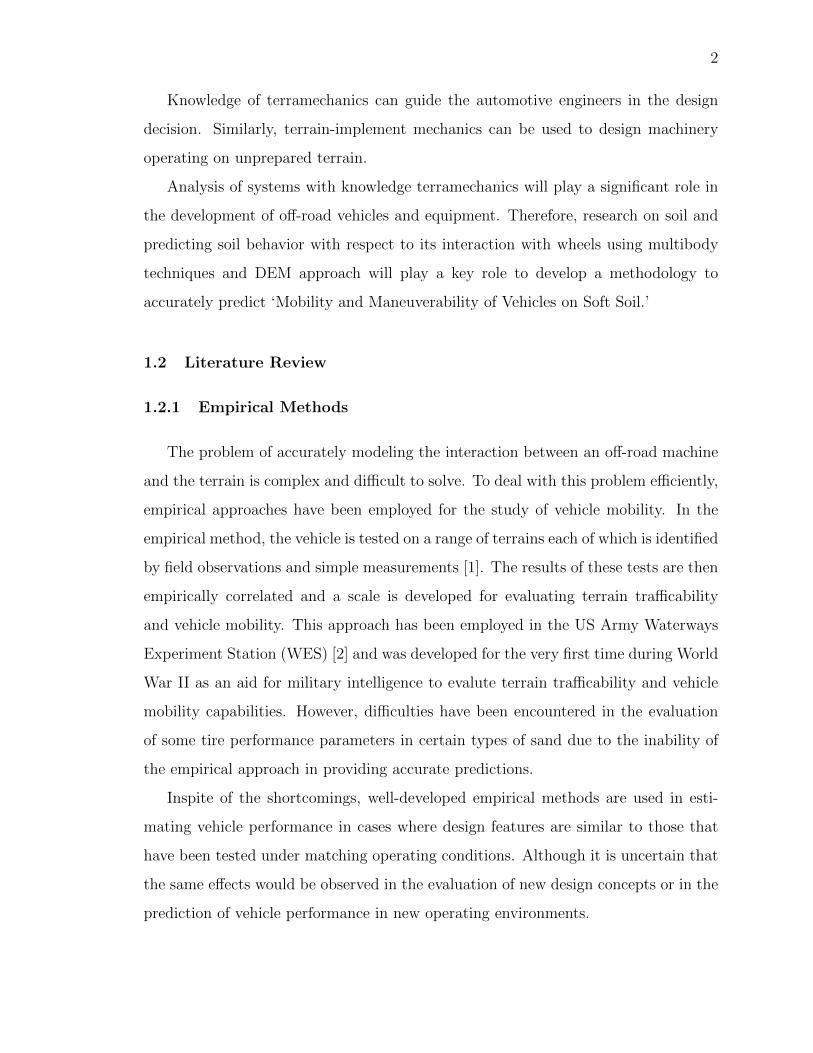
1.2.1 Empirical Methods

The problem of accurately modeling the interaction between an off-road machine

and the terrain is complex and difficult to solve. To deal with this problem efficiently,

empirical approaches have been employed for the study of vehicle mobility. In the

empirical method, the vehicle is tested on a range of terrains each of which is identified

by field observations and simple measurements [1]. The results of these tests are then

empirically correlated and a scale is developed for evaluating terrain trafficability

and vehicle mobility. This approach has been employed in the US Army Waterways

Experiment Station (WES) [2] and was developed for the very first time during World

War II as an aid for military intelligence to evalute terrain trafficability and vehicle

mobility capabilities. However, difficulties have been encountered in the evaluation

of some tire performance parameters in certain types of sand due to the inability of

the empirical approach in providing accurate predictions.

Inspite of the shortcomings, well-developed empirical methods are used in esti-

mating vehicle performance in cases where design features are similar to those that

have been tested under matching operating conditions. Although it is uncertain that

the same effects would be observed in the evaluation of new design concepts or in the

prediction of vehicle performance in new operating environments.

3

1.2.2 Lumped Parameters Parametric Analysis Methods

We will be looking into the mathematical model approach for the parametric

analysis of the performance of off-road vehicles in order to circumvent the limitations

of empirical methods mentioned earlier. A pioneering effort in this area was made by

Bekker [3] [4] [5]. Computer-aided methods which are based on lumped parameters

models for parametric analysis of the performance and design of tracked and off-road

wheeled vehicles include: methods for performance and design evaluation of vehicles

with flexible tracks (NTVPM), vehicles with long-pitch link tracks (RTVPM), and off-

road wheeled vehicles (NWVPM) [1]. These methods are based on the physical nature

of vehicle-terrain interaction and terramechanics principles and consider major design

features of the vehicle that affect its performance. Also, terrain characteristics, such

as pressure-sinkage, shearing characteristics and response to repetitive loading are

considered. These computer-aided methods are particularly suited for the evaluation

of competing designs, optimization of design parameters, and selection of vehicles for

a given mission and environment. They have been successfully used to assist off-road

vehicle manufacturers in the development of new products.

Bekker Method

M.G. Bekker, was studying terramechanics during the 1950s and 1960s, and cre-

ated semi-empirical equations for vehicle performance on soft soils which created the

foundation for many terramechanics studies [3] [4] [5]. The original Bekker equa-

tions are modified and improved to fit researches being performed now. The Bekker

method assumed the wheel-soil interface in a 2 dimensional plane, considereing the

wheel to be a simple circle operating on a flat leveled soil plane. Wheel dips into the

soil because of the applied normal load and slip s, creating an entry contact angle θf

and exit contact angle θr. Wheel slip ratio, which depends on the angular velocity ω,

the linear velocity vx, and the wheel radius r, is defined by

4

s = (ωr − vx)/vx (1)

Along the wheel-soil interface normal stresses σ and tangential stresses τ develop,

which can be integrated to find the forces acting on the wheel. The normal force,

drawbar force (sum of thrust and resistance forces), anddriving torque is defined by

Fnormal = rb

∫ θf

θr

(σcosθ + τsinθ) dθ (2)

Fdrawbar = rb

∫ θf

θr

(τcosθ − σsinθ) dθ (3)

Twheel = r2b

∫ θf

θr

τdθ (4)

where b is the wheel width.

Normal stress along the interface is assumed to be equivalent to the normal pres-

sure on a flat plate at the same sinkage z, the amount of vertical soil compression.

The function to calculate normal stress is defined by

σ = k

(z

bplate

)n(5)

where k and n are pressure-sinkage parameters, which can be determined through

plate-sinkage experiments, and bplate is the width of the flat plate. The equation for

sinkage has been modified somewhat to account for the bow-like shape of normal

stress that occurs along the wheel-soil interface [6] [7]. Sinkage along the interface is

split between the front and rear regions, defined by

z =

r (cosθ − cosθf ) θm ≤ θ ≤ θf

r (cosθeq − cosθf ) θr ≤ θ ≤ θm(6)

where the location of maximum stress θm and the equivalent front-region contact

angle θeq equal

θm = (a0 + a1s) θf (7)

5

Fig. 1.1. Mohr circle in terramechanics [1].

θeq = θf − (θf − θm)θ − θrθm − θr

(8)

The coefficients a0 and a1 are used to empirically adjust the location of maximum

stress according to wheel slip s and entry contact angle. The rear contact angle θr

was assumed to be zero for the purpose of this study.

τs>=0 = τres

(1− exp

(−|j|K

))τs<0 =

−τres(

1− exp(−|j|K

))θ ≥ θm

τres

(1− exp

(−|j|K

))θ < θm

(9)

where j is the shear displacement and K is the shear modulus coefficient [8] [9].

The residual shear stress τres is determined according to the Mohr-Coulomb failure

criteria, defined by

τres = c+ σtanφ (10)

where c is the soil cohesion and φ is the angle of internal friction, both of which can

be determined through soil tests. The shear displacement equation varies based on

the slip ratio and the location of the interface [8] [9] given by

js>=0 = r [(θf − θ)− (1− s) (sinθf − sinθ)]

js<0 =

r (1− s)

(θf − θ) sinθf−θmθf−θm

−sinθf + sinθ

θ ≥ θm

r [(θm − θ)− (1− s) (sinθm − sinθ)] θ < θm

(11)

6

The Bekker method has several advantages over terramechanics methods, includ-

ing computation speed. Many of the soil coefficients can be determined through

simple soil tests. Some parameters can only be determined if wheel test data is

available. The simplicity of the Bekker method creates several limitations. Model-

ing three-dimensional wheel-soil interaction requires significant modification to the

Bekker method to improve numerical accuracy with increased numerical terms.

Dynamic Bekker Method

The Dynamic Bekker method is an enhancement to Bekker method by including

multibody dynamics and irregular soil profile which is done considering the wheel

as a body with inertia, and discretizing the soil [10]. Therefore the Bekker stress

equations are applied to each region of the discretisized soil. The drawbar pull and

driving torque are provided by the Langrange multipliers that are calculated by the

constrained multibody dynamics problem. A vertical force is given at the wheel

center to produce desired normal load. The soil is modeled using a uniformly spaced

set of spheres, supported by nonlinear vertical springs. When the soil particles come

in contact with the wheel body, the nodes will be displaced creating soil normal

pressure.

1.2.3 Computational Methods

Computational methods like the finite element method (FEM) and the discrete

(distinct) element method (DEM) have proved beneficial for the analysis of vehicle-

terrain interaction due to the recent advancements made in computer technology and

the availability of commercial computer codes. They have the potential of providing a

tool to examine in detail certain aspects of the mechanics of vehicle terrain interaction

[11].

Predictions of tire performance based on these computational methods have been

shown to be in qualitative agreement with experimental data on certain types of ter-

7

rain. For a complex mechanical track system, its interaction with the terrain involves

not only the part of the track system in contact with the terrain, but also other

factors, such as roadwheel system configuration, suspension characteristics, locations

of the sprocket and idler, initial track tension, arrangement of the supporting rollers

on the top run of track, etc. To make the analysis responsive to the finite element

method, the track usually has to be simplified to a rigid footing with either uniform

or trapezoidal form of normal pressure distribution [8] [12]. In many cases, the ratio

of the shear stress to normal pressure also needs to be specified.

Discrete Element Method

The discrete element method (DEM) implemented by lumping the soil particles

into larger particles, defined by their size, shape, position, velocity, and orientation

[9]. A basic DEM model will assume each particle is attached to an adjacent particle

with normal spring and damper, tangential spring and damper. These contacting ele-

ments are assumed in particle-particle contact (Figure 1.2) and also particle-machine

surface contact (Figure 1.3). But it is to be noted that maximum tangential force

is limited by the product of the coefficient of friction and the normal force [1]. In

Figure 1.2 and Figure 1.3 the spring elements in both the directions cannot sustain

tensile forces, because there is no tensile joint in between them as a result of that

the effect of cohesion and adhesion is neglected [1]. When Particle collision generates

forces and torques using explicit equations. Modeling the soil using this discretized

approach allows accounting for significant soil deformation and change in properties

due to change in soil structure and non-homogenity [9]. Many researchers have found

that when contact is described by only normal and tangential friction forces, more

complicated particle shapes like ellipsoids, poly-ellipsoids, polyhedrals can better re-

produce soil behavior compared to spheres. Particle collision generates reaction forces

which are determind by parameters like length and velocity of particle-particle over-

lap [13]. In the general DEM [14] [15] inter-particle forces include: normal contact

forces (deflection and/or velocity dependent forces which prevent the particles from

8

into penetrating each other), attraction forces, tangential contact forces (friction and

viscous forces) and distance dependent forces (gravity, electrostatic and magnetic

forces). Particles can be either point particles or rigid body type particles. They can

also be spherical, cubical or of any arbitrary shape. References [16] [17] were the first

to use DEM to model soils using spherical particles for vehicle mobility applications.

In [16] [17] the inter-particle force model included friction and particle stiffness but

did not include cohesive (attractive) forces and plasticity. The DEM technique de-

veloped in [16] [17] was also extended to non-spherical ellipsoid particles. Cubical

rigid body particles were used with a force model that includes normal particle stiff-

ness/damping, tangential viscous and Coulomb friction forces in Wasfy et al. [30,

31].

Fig. 1.2. Particle-to-particle normal and tangential contact properties. [1]

Fig. 1.3. Particle-to-surface Normal and Tangential contact properties. [1]

9

Finite Element Method

A Lagrangian finite element mesh along with an elastovisco-plastic constitutive

material model such as Drucker–Prager model [18] are used for modeling the soil.

There are a few disadvantages to this method. Firstly, it cannot capture soil sep-

aration/reattachment. Secondly, soil deformation/flow require remeshing and re-

interpolating the solution field to the new mesh which is computationally expensive

and also the accurcy is compromised. On the other hand, the volume-of-fluid method

[19] [20] [21] allows the use of a finite element model while accounting for soil separa-

tion/reattachment. Each element has a VOF value between 0 (for empty elements)

and 1 (for elements completely filled with fluid/soil). The free surface for each ele-

ment is reconstructed using piecewise-linear planar segments that are calculated from

the VOF value of the element and the VOF values of the neighboring elements. This

VOF approach requires the use of an Arbitrary Lagrangian-Eulerian formulation that

makes it very difficult to account for soil cohesion and plastic deformation. The finite

element method is based on the assumption that the terrain is a continuum which

poses limitations in simulating large, discontinuous terrain deformation which often

occurs in off-road operations.

1.3 Objectives and Contributions

In this thesis, a three-dimensional DEM model is used along with multibody dy-

namics model of previously published experiments which include direct shear stress,

penetroplate pressure-sinkage test, and rigid-wheel soil interface test to predict vari-

ous soil characteristics. The DEM model, that is used to model the granular material,

supports arbitrarily shaped 3D particles, where each particle is modeled as a rigid

body. The particle shape can be represented using: a superquadric surface, a polyg-

onal surface or an assembly of spheres rigidly fixed to the rigid body. The experi-

mental setup is modeled using rigid bodies, joints and actuators. The rigid bodies’

rotational equations of motion are written in a body fixed frame with the total rigid

10

body rotation matrix updated each time step using incremental rotations [22]. An

asperity-based Coulomb friction model is used to model tangential friction forces [23]

between the particles and each other and between the particles and another rigid

surface. The friction model along with the accurate representation of the particle

shape allows the formation of a stable (static) particle pile and accurate behavior

of particles during sliding. A penalty contact technique, with a penalty spring and

an asymmetric damper, is used to model normal contact forces. Tangential damping

(viscous) forces can also be included in the model. The Eulerian grid space decompo-

sition along with a bounding sphere contact check used in [24] is used in the present

model to speed inter-particle contact detection. Contact between rigid bodies (in-

cluding the particles and rigid components) is detected using a binary tree contact

search algorithm which allows fast contact search. A penalty formulation is also used

for modeling joint constraints including spherical, revolute, cylindrical and prismatic

joints [25]. The equations of motion are integrated using a time accurate explicit

predictor-corrector solution procedure.

The main contributions of this thesis are:

• Creating and tuning a non-cohesive DEM soil model by simulating the previ-

ously performed and published experiments (direct shear stress test, pressure-

sinkage penetrolplate test, rigid wheel soil interface test) in multibody dynamics

environment and comparing the results against previously published research

work with the same experiments. Each test is a measure of specific mechani-

cal characteristics of the soil under various loading conditions. Shear strength

of the soil as a function of normal load help to understand shearing of the

soil under a vehicle wheel contact patch causing loss of traction. Penetroplate

pressure-sinkage test is used to calibrate and validate friction and shear strength

characteristics of the soil. The rigid wheel-soil interaction test is used to predict

drawbar pull force and wheel torque vs. slip percentage and normal stress for

a rigid wheel.

11

• The DEM soil model is used in the simulation of a full vehicle MBD model on

a sand terrain.

1.4 Tools Used

In this research, the main CAE software tool which was used to create the all the

MBD models of the experiments and DEM soil models: DIS (Dynamic Interactions

Simulator) [26].DIS is a commercial multibody dynamics code that can be used to

simulate mechanical systems which include multiple rigid and flexible components

that can come into contact with each other and that are connected using various

types of joints. The code also allows adding linear and rotary actuators and the

control systems used along with those actuators. The DIS code uses a computationally

efficient explicit predictor-corrector time integration method to solve the equations

of motion. DIS has been used to predict the dynamic response in many multibody

dynamic applications including automotive, aerospace and industrial applications.

Further details about the formulation and solution procedure used in the DIS code

are provided in next chapter.

1.5 Thesis Organization

This thesis is organized as follows. In Chapter 2, the multibody dynamics for-

mulation and solution procedure used in the DIS code are presented. In Section 2.1,

the translational and rotational semi-discrete equations of motion are presented. In

Section 2.2, the contact model including the normal force model and tangential asper-

ity friction force model; contact search algorithm; and particle shape representations

are presented. In Section 2.3, the penalty algorithm for imposing joint constraints is

presented. Linear and rotary actuators models are outlined in Section 2.4. In Section

2.5, the explicit solution procedure is presented. In the following chapters that are

Chapter 3, 4 and 5 the experimental and simulation models are explained and the

simulation results are compared with previously published experiments for: direct-

12

shear test (Chapter 3), penetroplate test (Chapter 4), rigid-wheel soil interface test

(Chapter 5). In Chapter 6, a practical application of the tuned sand-type soil model

is shown, with a simulation of a HUMVEE-type vehicle driving over a unpaved track

containing the soil model. Finally, concluding remarks and future scope of research

are given in Chapter 7.

13

2. MULTIBODY DYNAMICS FORMULATION

In this chapter, the equations of motion along with the time-integration rule used

in the DIS [26] code are outlined. In the subsequent equations, the following conven-

tions are used:

• Indicial notations

• Einstein summation convention for repeated subscript is used

• Upper case subscript indices represent node numbers

• Lower case subscript indices represent vector component number.

• The superscript denotes time.

• A superposed dot denotes a time derivative.

2.1 Equations of Motion

A rigid body is modeled as a finite element node located at the rigid body’s center

of mass. An algorithm used for generating and integrating the equations of motion

for three-dimensional rigid bodies using an explicit finite element [22]. Each node

(rigid body) has 3 translational degrees-of-freedom and a rotational matrix is defined

with respect to the global inertial.

The translational equations of motion for all nodes are with respect to the global

inertial reference frame which is obtained by assembling the individual node equations

which can be written as

MK xtki = F t

sKi+ F t

aKi(12)

14

where t is the real time, K is the global node, i is the coordinate number (i = 1; 2; 3),

MK is the lumped mass of node K, x is the vector of nodal cartesian coordinates with

respect to the global inertial reference frame, x is the vector of nodal accelerations with

respect to the global inertial reference frame, Fs is the vector of internal structural

forces, and Fa is the vector of externally applied forces, which include surface forces

and body forces. For each rigid body (node), a body-fixed material frame is defined.

This origin of the body frame is located at the body’s center of mass. The mass of

the body is concentrated at the center of mass and the inertia of the body is given by

the inertia tensor Iij defined with respect to the body frame. The orientation of the

body-frame is given by Rt0k which is the rotation matrix relative to the global inertial

frame at time t0. The rotational equations of motions are written for each node with

respect to its body-fixed material frames

IKij θtKj = T tski + T taki − (θtKi × (IKij θ

tKj))Ki (13)

where Ik is the inertia tensor of rigid body K, θkjand θkj are the angular acceleration

and velocity vectors components for rigid body K relative to its material frame in

direction j (j = 1; 2; 3),TsKi are the components of the vector of internal torque at

node K in direction i, and TaKi are the components of the vector of applied torque.

The summation convention is used only for the lower case indices i and j. Since, the

rigid body rotational equations of motion are written in a body (material) frame, the

inertia tensor IK is constant.

The trapezoidal rule is used as the time integration formula for solving 24 for the

global nodal positions x :

xtKj = xt−∆tKj + 0.5∆t

(xtKj + xt−∆t

Kj

)xtKj = xt−∆t

Kj + 0.5∆t(xtKj + xt−∆t

Kj

) (14)

where ∆t is the time step. The trapezoidal rule has been used for the time integration

formula for the nodal rotation increments

15

θtKj = θt−∆tKj + 0.5∆t

(θtKj + θt−∆t

Kj

)∆θtKj = 0.5∆t

(θtKj + θt−∆t

Kj

) (15)

where ∆θKj is the incremental rotation angles around the three body axes for the body

K. Thus, the rotational equations of motion are integrated to yield the incremental

rotation angles. The rotation matrix of body K (RK) is updated using the rotation

matrix corresponding to the incremental rotation angles

RtK = Rt−∆t

K R(∆θtKi

)(16)

where R( ∆θtKi) is the rotation matrix corresponding to the incremental rotation an-

gles from Equation (16). The explicit solution procedure used for solving Equations

12-19 along with constraint equations. The constraint equations are generally alge-

braic equations, which describe the position or velocity of some of the nodes. They

include

• Contact/impact constraints (Section 2.2):

f ({x}) ≥ 0 (17)

• Joint constraints:

f ({x}) = 0 (18)

• Prescribed motion constraints:

f ({x} , t) = 0 (19)

2.2 Contact Model

Normal contact constraints between contact point on a rigid body and a surface

on another rigid body. The penalty method has been used [22] [27]. The firstly it is

important to find the position and velocity of a contact point on a rigid body. The

global position xGp and velocity xGp of a contact point are given by

16

Fig. 2.1. Location of a point on a rigid body with respect to the localbody frame (XLP) and the global reference frame (XGP) [28].

xGpi = XBi+RBij

xLpj

xGpi = XBi+RBij

(WBF × xLp)j(20)

where XB and XB are the global position and velocity vectors of the rigid body’s

frame, RB is the rotation matrix of the rigid body relative to the global reference

frame, WB is the rigid body’s angular velocity vector relative to its local frame,

and xLp is the position of the contact point relative to the rigid body’s frame. The

contact force Fc at each contact point is the sum of the normal contact force (Fn)

and tangential friction force (Ft):

Fci = Fti + Fni(21)

Fc is transferred as a force to the center of the rigid body (the node) using

Fi = Fci (22)

Ti = (xLP i ×RBF jiFci) (23)

xLP j= RBF ji

(xGpi −XBF i

)(24)

where Fi is the contact force at the CG of the rigid body (center of the body frame),

Ti is the contact moment on the rigid body, xLcp is the position of the contact point

17

relative to the rigid body’s frame and xGcp is the position of the contact point relative

to the global reference frame. Similarly, the negative of this force is transferred to

the center of the contacting rigid body as a force and moment.

2.2.1 Penalty Normal Contact Model

The penalty technique is used for insuring that particles or rigid bodies do not

interpenetrate. A normal reaction force (Fn) is generated when a node penetrates in

a contact body whose magnitude is proportional to the penetration distance. The

force is given by:

|fn| = AKpd+ A

Cpd d ≥ 0

SpCpd d < 0(25)

d = vreli (26)

vni= dni

(27)

Vti = vreli − vni(28)

where A is the area associated with the contact point, Kp and Cp are the penalty

stiffness and damping coefficients per unit area respectively; d is the closest distance

between the node and the contact surface as shown in Figure 2.2; d is the signed

time rate of change of d ; Sp is the separation damping factor between 0 and 1 which

determines the amount of sticking between the contact node and the contact surface

at the node (leaving the body); vreli is the relative velocity vector between the contact

point and the contact surface; −→n is the normal to the surface, vniis the velocity vector

in the direction of −→n , and −→v ti is the tangential velocity vector.

2.2.2 Asperity Friction Model

An asperity-spring friction model is used to model contact and joint friction [23].

The model approximates asperity friction where friction forces between two rough

18

Fig. 2.2. Contact surface and contact node [28]

surfaces in contact arise due to the interaction of the surface asperities Figure 2.3.

The tangential friction contact force vector transmitted to the contact body at the

contact point. (Fti) is given by:

Fti = ti |Ft| (29)

ti = vti/ |−→vt | (30)

where ti is a unit vector along the tangential contact direction. The asperity friction

model is used along with the normal force to calculate the tangential friction force

(|Ft|) [23]. When two surfaces are in static (stick) contact, the surface asperities act

like tangential springs. When a tangential force is applied, the springs elastically

deform and pull the surfaces to their original position. If the tangential force is

large enough, the surface asperities yield (i.e. the springs break) allowing sliding to

occur between the two surfaces. The breakaway force is proportional to the normal

contact pressure. In addition, when the two surfaces are sliding past each other, the

asperities provide resistance to the motion that is a function of the sliding velocity

and acceleration, and the normal contact pressure. Figure 2.3 [29] shows a schematic

diagram of the asperity friction model. It is composed of a simple piece-wise linear

velocity-dependent approximate Coulomb friction element in parallel with a variable

anchor point spring. In order to connect two points on two bodies using an asperity

19

Fig. 2.3. Asperity-based physical interpretation of friction [28]

Fig. 2.4. Asperity spring friction model where Ft is the tangential fric-tion force, Fn is the normal force, µk is the kinetic friction coefficient,and vrt is the relative tangential velocity between the two points ofcontact [28]

spring, the model must keep track of which rigid bodies are in contact and of the local

position vectors of the asperity spring anchor points on the two contacting bodies. It

also must keep track of the corresponding contact points on the two contact bodies.

20

2.2.3 Inter-Particle Contact Search

Another key component of the DEM is search and detection of inter-particle con-

tacts. In [29] a space decomposition contact search algorithm was developed. This

algorithm is implemented to search for particle contact. The steps of the algorithm

are as follows:

1. The space where the particles can move is decomposed into a Cartesian Eulerian

volume grid of equally sized boxes (Figure 2.5).

2. We loop over all the particles. For each particle, the grid boxes that intersect

the particle are found. The minimum and maximum vertical and horizontal grid

numbers of a particle can be easily found knowing the position of the center of

the particle and the bounding box of the particle. In addition, each grid box

has a list of particles that it intersects. Thus, in the same loop for each grid

box that intersects the particle we add the particle to the grid box.

3. For each particle the neighbohood particles can come into contact with a particle

is generated. This list consists of the particles that intersect the boxes that the

particle intersects.

4. For each particle, the distance between the center of the particle and the center

of a neighboring particle is calculated. If that distance is larger than the sum of

bounding sphere radii of the two particles, then the particles are not in contact.

Otherwise, contact point detection is carried out to find the contact point (if

any).

5. The algorithm keeps track of the boxes that contain particles and those are

initialized to zero particles each time step. This is important since the number

of Cartesian boxes is typically much larger than the number of particles [30].

For example in Figure 2.5 :

Particle 6 intersects vertical grids 9 to 11 and horizontal grids 4 to 5.

21

Fig. 2.5. Cartesian grid domain decomposition [30]

Grid (9,4) intersects particles: 3, 4, 5, 6.

Grid (9,5) intersects particles: 5, 6. 7

Grid (10,4) intersects particles: 4, 6

Grid (10, 5) intersects particles: 6

Grid (11, 4) intersects particles: 4, 6, 8, 10

Grid (11,5) intersects particles: 6, 8, 9, 11

Thus, particle 6 neighbors are: particles: 3, 4, 5, 7, 8, 9, 10, 11.

The main algorithm loop runs over the number of particles N. Thus, the com-

plexity is O(N). The additional bounding sphere search quickly eliminates most of

the neighboring particles thus the particles that the most computationally expensive

contact point detection is carried over are the neighboring particles that have a very

high likelihood of being in contact with the particle.

2.2.4 Contact Point Search

Superquadric and Spherical Surfaces Contact Search – The detection is performed

between contact points on a contact surface of a rigid body, called the master contact

22

surface, and a surface of another rigid body, called the slave contact surface [31]. The

slave contact surface can be: a superquadric surface (Figure 2.6) or a collection of

bounding spheres (Figure 2.8). A superquadric surface centered at point (0, 0, 0) is

defined by:

(x1

r1

)p1+

(x2

r2

)p2+

(x3

r3

)p3= 1 (31)

where xi is the coordinate of a point on the surface, ri is the radius in direction i, and

Pi is the exponent in direction i. If the master contact point coordinates xci in the

slave contact body frame satisfies the following condition:(x1

r1

)p1+

(x2

r2

)p2+

(x3

r3

)p3≤ 1 (32)

Then the master contact point is inside the contact slave body. Similarly, if the

slave contact surface is a collection of spheres (Figure 2.7) then Equation 32 can be

used to detect contact if the contact point coordinates xci are calculated in the local

frame of each sphere on the slave contact body. In the case of a sphere, p1 = p2 = p3

= 2, and r1 = r2 = r3 = r . In that case Equation 39 becomes:

(xc1)2 + (xc2)

2 + (xc3)2 ≤ r2 (33)

where r is the radius of the sphere.

Fig. 2.6. Particle of cubical shape modeled using superquadric withN = 3 (left) and N = 8 (right) [31]

The sand particle shape model used in the rest of this thesis is the glued sphere

model in Figure 2.7. Eight spheres are glued to form a cubical-like particle.

Polygonal Surface Contact Search – This contact model is used to model contact

between rigid bodies and the particles. If the slave contact surface is a polygonal

23

Fig. 2.7. Particle of cubical shape modeled using 8 spheres [31]

surface (see Figures 2.8) binary tree contact search algorithm is employed to detect

contact between a contact point of the master surface and the polygons of the slave

surface. [31]. Following are the initial steps of the algorithm:

• Each slave polygonal contact surface is divided into 2 blocks of polygons. The

bounding box is found for each block and again each block is further divided

and bounding boxes found. This recursive division continues until there is only

one polygon in a box.

• For each master contact sphere, the radius of the contact sphere is added to

the size of the bounding box, then it is checked if the center point of the sphere

is inside a bounding box. If it is not, then all the points inside that sphere

are concluded to be not in contact with the surface. Otherwise it needs to be

determined if the point is inside either box. If it is, then the sub-contact spheres

are checked. If a contact point is found to be inside the lowest level bounding

box, then a more computationally intensive contact algorithm between a point

and a polygon is used to determine the depth of contact and the local position

of the contact point on the polygon.

2.3 Joint Constraints

A joint connects two rigid bodies. A joint imposes motion constraints between

points on two rigid bodies. All rigid bodies consist of numerous connection points,

24

Fig. 2.8. Particle of cubical shape modeled using a polygonal surface [31].

these connection points are the points where joints are attached and it does not add

DOFs to the system. The position and velocity of a connection point are given by

Equations 34 and 35, respectively, where xLP is the position of the connection point

relative to the body’s frame and xGP and xGP are the position and velocity of the

connection point relative to the global reference frame.

2.3.1 Revolute Joints

A revolute joint constrains three translational DOFs and two rotational DOFs

between two rigid bodies, thus leaving only one rotational DOF free between the

bodies. Revolute joints can be modeled by placing two spherical joints along a line.

Therefore, the same mathematical methods which are used for the spherical joints

can be used to define revolute joints.

2.3.2 Prismatic Joints

A prismatic joint constrains two translational and three rotational DOFs between

two rigid bodies and leaves only one translational DOF free Figures 2.14 and 2.15.

Prismatic joints can be modeled by placing two cylindrical joints in parallel [30].

25

Fig. 2.9. Prismatic joint in 2D

2.4 Actuators

2.4.1 Linear Actuator

A linear actuator connects two points on two rigid bodies (Figure 2.16). Using a

PD controller, the force F is generated by the actuator is given by:

F = K (l − ldes) + c

(lilil− ides

)(34)

li = xtc1i − xtc2i

(35)

li = xtc1i − xtc2i

(36)

l =√l21 + l22 + l23 (37)

where xtc1i is the position of the first point on the first body and xtc2i is the position of

the second point on the second body, both with respect to the global reference frame;

K is the controller proportional gain, c is the controller derivative gain, ldes is the

desired length of the actuator, l is the current length of the actuator, and is F the

actuator force vector [28] [32]. The actuator force is transferred to the rigid bodies

center as force and moment using Equations 37 and 38.

2.4.2 Rotational Actuator

A rotational actuator connects three points on two rigid bodies (Figure 2.11).

Two of the points are on one rigid body and the remaining point is on the second

26

Fig. 2.10. Linear actuator connecting two points [28] [32]

Fig. 2.11. Rotational actuator connecting three points [28] [32]

rigid body. Using a PD controller the torque T generated by the actuator is given

by:

T = k (θ − θdes) + c(θ − θdes

)(38)

where θ is the current angle of the actuator, θdes is the desired angle, k is the propor-

tional gain and c is the derivative gain. The rotary spring forces are transferred to

the rigid bodies’ center as force and moment using Equations 39, 40.

2.5 Explicit Solution Procedure

The solution fields for modeling multibody systems are defined at the model nodes

wherein a rigid body is modeled as one finite element node. The solutions fields are:

27

• Translational positions

• Translational velocities

• Translational accelerations

• Rotational matrices

• Rotational velocities

• Rotational accelerations

The explicit time integration procedure predicts the time evolution of the above

response quantities. The procedure described below achieves near linear speed-up

with the number of processors on shared memory parallel computers. The procedure

is implemented in the DIS [26] (Dynamic Interactions Simulator) commercial software

code and is outlined below:

1. Prepare the run:

a. Set the initial conditions for the solution fields mentioned above.

b. Create a list of all the finite elements that includes the master contact

surfaces.

c. Create a list of elements that will run on each processor. This is done

using an algorithm which tries to make the computational cost on each

processor equal.

d. Create a list of all the prescribed motion constraints.

e. Calculate the solid masses for each finite element node by looping through

the list of finite elements. Note that the masses are fixed in time.

f. Loop over all the elements and find the minimum time step for the explicit

solution procedure.

2. Loop over the solution time and increment the time by t each step while doing

the following:

28

a. Set the nodal values at the last time step to be equal to the current nodal

values for all solution fields.

b. Do 2 iterations (a predictor iteration and a corrector iteration) of the

following:

i. Initialize the nodal forces and moments to zero.

ii. Perform the particle Contact search algorithm

iii. Calculate the nodal forces and moments by looping through all the

elements while calculating and assembling the element nodal forces.

This is the most computationally intensive step. This step is done in

parallel by running each list of elements identified in step 1.c on one

processor.

iv. Find the nodal values at the current time step using semi-discrete

equations of motion and the trapezoidal time integration rule.

v. Execute the prescribed motion constraints which set the nodal value(s)

to prescribed values.

vi. Go to beginning of step 2.

29

3. DIRECT SHEAR TEST

The shear stress-displacement model is intended for the identification of the shear

strength specifically the cohesion, angle of friction, shear modulus which will be help-

ful for prediction of the tractive performance of the vehicles running over unprepared

soils. Bekker [3] proposed Eq. (2.15) to describe the shear stress displacement rela-

tionship for brittle soils which contains a hump of maximum shear stress [32].

τ

τmax=

e

(−K2+

√K2

2−1)K1j − e

(−K2−

√K2

2−1)K1j

e

(−K2+

√K2

2−1)K1j0 − e

(−K2−

√K2

2−1)K1j0

(39)

where,

τ = shear stress

τmax = maximum shear stress

K1 = empirical parameter in the Bekker shear equation

K2 = empirical parameter in the Bekker shear equation

j = shear displacement

j0 = shear displacement at τmax

Janosi and Hanamoto [33] [34] established a modified shear stress-displacement

equation based on the Bekker equation. This modified equation is widely used due

to the simplicity that only one constant is included.

τ

τmax= 1− e(−j/K) (40)

where K is the shear deformation modulus

3.1 Experiment and Simulation

The test setup was ASTM International Standard Test Method for Direct Shear

Test. [10] The rig consists of three main parts: the carriage and loading box, the motor

assembly, and the load cell. The carriage is fitted with a loading box, in which the

30

Fig. 3.1. Direct shear stress experimental setup [36]

test material sits. Normal load by putting known weight is given on the loading box.

Three different weights have been used in the test and the simulation. Three different

soil specimens have been used. Simulation soil model is tuned to co-relate average test

results of the three samples. The loading box consists of two halves that are allowed

to slide freely, the lower box is given linear displacement in a controlled fashion by a

motor in the test rig which is emulated by a linear actuator in the simulation and the

displacement and resistive force by the soil is measured. The resistive force exerted

tangentially by the soil against the motion of the lower box is measured to create plots

of shear stress as a function of shear displacement. The shear stress vs. displacement

relationship levels off when the material stops expanding or contracting, and when

inter-particle bonds are broken. The shear stress remains constant while the shear

displacement increases may be called the critical state, steady state, or residual shear

stress [35].

In the simulation it was important to randomize the DEM soil particles to emulate

actual condition therefore the soil particle grid box is dropped at a three dimensional

angle and the lower box was an attached to a shaker actuator to shake the box and

get all the soil particle oriented randomly.

31

Fig. 3.2. MBD simulation model hierarchy

Table 3.1.MBD model properties for direct shear stress simulation

Number of rigid bodies 4

Number of prismatic joints 3

Number of linear actuator 3

3.2 Results and Explanation:

The multibody dynamics model of the direct shear stress experiment consist of

as shown in Figure 3.2 ground, bottom box, top box, lid and the particles. Table 1

states MBD model properties which consist of 4 rigid bodies, 3 prismatic joints and

3 linear actuators. As shown in Figure 3.3 the linear actuator acting through the

prismatic joint of the lid is connected to the top box. The Lid actuator is activated

once the particles box grid falls and settles inside the box. The particle box has been

given an initial three dimensional angle so that when it falls the particles are well

randomized. The total box size used to contain the particles is 60mm x 60mm x

50mm which are the specifications similar to the experiment. The lid is given the

normal loads of 6.2 kg, 16.2 kg and 26.2 kg as performed in the experiment. Once

the lid reached the particle top surface and stabilized the linear actuator of the top

box starts moving the top box linearly relative to the bottom box. The shear force

or the resistance force exerted by the particle is measured by a force sensor. All the

stages of the simulations are shown in Figure 3.4.

32

Fig. 3.3. Joints and actuators in the MBD model of direct shear stress test

Fig. 3.4. Snapshots of the direct shear stress test experiment

Fig. 3.5. DEM particle model inside IVRESS showing number ofparticles and particle radius

33

Fig. 3.6. IVRESS snapshot showing particle-particle contact properties

34

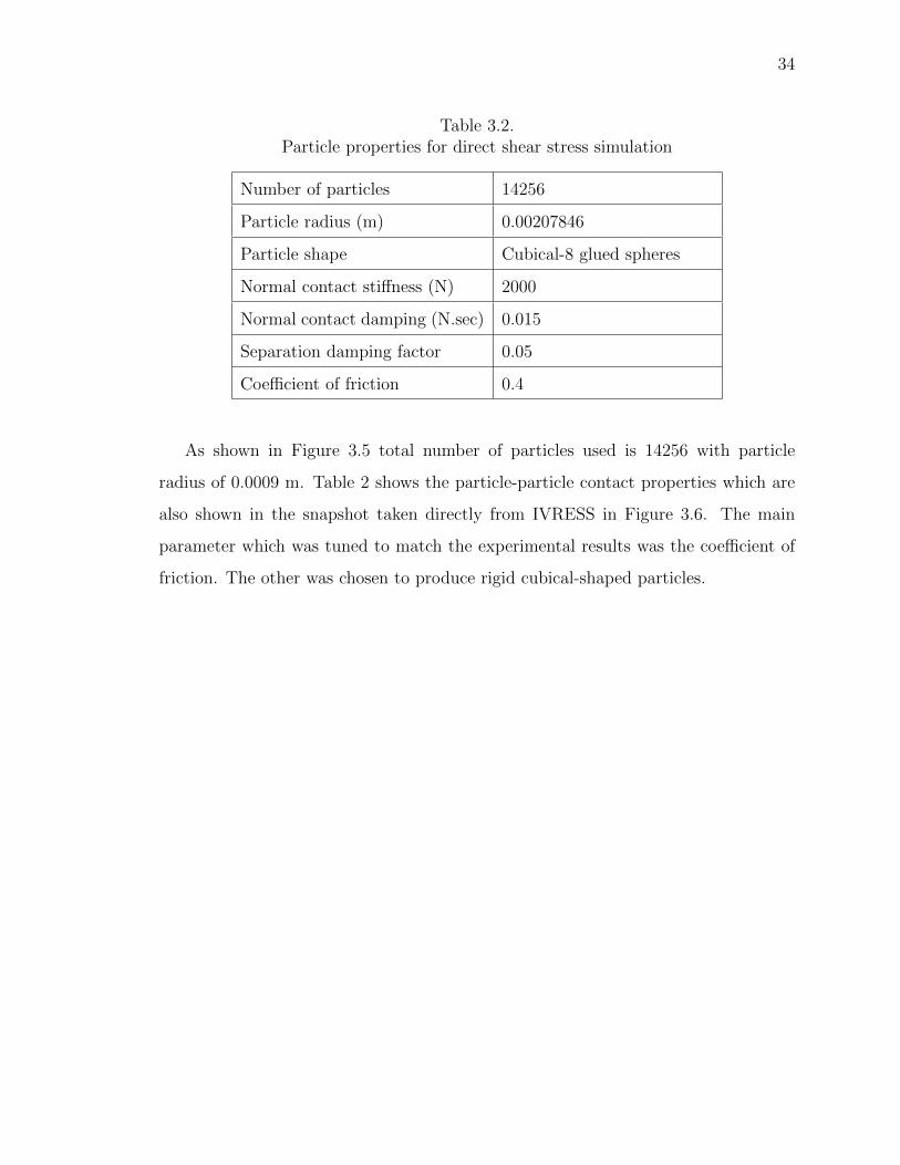
Table 3.2.Particle properties for direct shear stress simulation

Number of particles 14256

Particle radius (m) 0.00207846

Particle shape Cubical-8 glued spheres

Normal contact stiffness (N) 2000

Normal contact damping (N.sec) 0.015

Separation damping factor 0.05

Coefficient of friction 0.4

As shown in Figure 3.5 total number of particles used is 14256 with particle

radius of 0.0009 m. Table 2 shows the particle-particle contact properties which are

also shown in the snapshot taken directly from IVRESS in Figure 3.6. The main

parameter which was tuned to match the experimental results was the coefficient of

friction. The other was chosen to produce rigid cubical-shaped particles.

35

Direct Shear vs. Displacement Graphs:

Fig. 3.7. Comparison between simulation and test results with normalload of 16kPa [36]

In Figure 3.7 at load at 16kPa (6.2kg) the DEM soil model’s shear stress follows

the mean trend of the three soil sample in the experiment.

36


37


In Figure 3.8 and Figure 3.9 at load at 44kPa (16.2kg) and 71kpa (26.2kg) the

shear stress of DEM soil model has a lower initial slope than the experiment and the

stead-state shear stress is slightly higher than the experiment. The slope difference

can be due to the different speed shearing and the fact that the physical particles size

is much smaller than the size of the DEM particles.

38

Direct Shear vs. Normal Load Graph:

Fig. 3.10. Maximum shear stress plot of all the three simulations withvarying normal load

Figure 3.10 confirms the soil is non-cohesive as cohesivity (c) is found to be zero

and angle of friction (phi) is 38.043 degrees compared to 34.2 degrees and 43.5 degrees

of the low and high density soil sample used in the experiment.

Table 3.3.Maximum direct shear stress at different normal load

Normal Load(kPa) Max Shear(kPa)

16.895 13.48302778

44.145 33.79444444

71.395 56.12888889

Phi(deg) 38.043

c 0

39

4. PRESSURE-SINKAGE TEST

The first step for a semi-empirical method is to estimate the stress distribution (both

normal and shear stresses) developed at the interface between a plate and the soil

surface as a result it helps in predicting the load bearing property of the soil. The

normal stress is calculated from the pressure-sinkage equation originally introduced

by Bekker [4] and later modified by Reece (3.1),

p =(ck

′

c + γsbk′

ϕ

)(z/b)n (41)

where,

p = pressure normal to the sinkage plate

z = sinkage

n = sinkage index

c = soil cohesion

γ = soil density

k′c = cohesion dependent soil coefficient

k′ϕ = frictional dependent soil coefficient

b = parameter related to the geometry of the penetrometer (the smaller linear

dimension for rectangular plates)

The equation is a modified version of the Bekker sinkage-pressure equation (2.2),

also known as Bekker-Reece equation, where the ratio z/b is introduced for two

reasons: make the parameters kc and kϕ dimensionless and provide a single equation

that accounts for different plate shapes. The exponent n, is crucial because it defines

the trend of the relationship. Most soils behave almost linearly having n in the

range of 0.8 to 1.2. The density γ can be readily obtained while the cohesion c is

usually calculated through a series of uni-axial and tri-axial compression tests. The

sinkage index n, and the constants kc and kϕ are obtained using a bevameter or a

40

penetrometer. These devices apply a constantly increasing load on a plate which

is pushed perpendicularly down into the terrain. At the same time the sinkage is

measured and the experimental data points are assumed to be represented by sinkage

z and normal pressure σn are recorded. The experimental data is then fitted with

(3.1).

4.1 Experiment and Simulation

Pressure-sinkage experiment as mentioned above is performed to seek soils capa-

bility to react with normal pressure when a plate pushed into it at a constant velocity.

As a result it is important to tune the DEM soil model in the Multibody Dynamics

tool to get close co-relation between the test and simulation to emulate an accurate

model of the soil specimen.

The test rig [37] consists of a pressure plate which is connected to a force sensor

that senses normal force applied on the pressure plate surface. The whole setup is

connected to a linear actuator which pushes the pressure plate into a soil specimen

bath. In the simulation we remained careful selecting the soil bath size to avoid edge

affects causing soil hardening. Also, depth of the soil so selected that it has enough

clearance below the soil even after full travel of the actuator. In the simulation

before the pressure plate is activated we get the soil top surface smoothened to avoid

disturbances in the force sensor data.

In the experimental setup the pressure plates are made of Aluminum, therefore

minimizing friction between plate and sand. The constant velocity at which the

pressure plate is pushed down is 10mm/s. There is little disturbances in the velocity

during the experiment but it is assumed negligible in simulation and constant velocity

is provided to the pressure plate by the linear actuator.

In the experiment, various widths of pressure plates hae been used to accurately

understand the variation of normal pressure with change in the contact area. Simi-

larly, we have captured the same in simulation and tried to achieve similar results.

41

Fig. 4.1. Pressure sinkage penetroplate experimental setup [36]

42

Table 4.1.MBD model properties for pressure-sinkage penetroplate simulation




4.2 Results and Explanation


The multibody dynamics model of the pressure-sinkage experiment with penetro-

plate consist of the ground, bottom box, penetroplate, top box and DEM particles as

in Figure 4.2 and Table 4. Similar to the direct shear stress experiment the particle

box is dropped into the box space of 0.25m x 0.20m x 0.44m at a three dimensional

angle. The box space is so selected to reduce the computational time yet avoid edge

affect on the simulation results. Then the lid gets activated throught the linear ac-

tuator and drops to the particle surface and make the top surface even. Similarly

the penetroplate gets activated falls on the particle surface from there on it follows

a steady speed of 10 mm/s and the normal force to the penetroplate bottom surface

exerted by the particles is recorded by the force sensor. The simulation similar to the

experiment is repeated with 3 different penetroplate sizes that is 130mm x 30mm x

10mm; 130mm x 50mm x 10mm; and 130mm x 70mm x 10mm. A total number of

particles used 209664 with particle radius of 0.00186m (Figure 4.5).

43

Fig. 4.3. Joints and actuators in the MBD model of penetroplatepressure sinkage test

Table 4.2.Particle properties for pressure-sinkage penetroplate simulation

Number of particles 209664

Particle radius (m) 0.00186

Particle shape Cuibcal-8 glued spheres

Normal contact stiffness (N) 2000

Normal contact damping (N.sec) 0.015



44

Fig. 4.4. Snapshot of penetroplate pressure sinkage simulation


As it can be seen from Figure 4.6 and Table 5 the particle-particle contact prop-

erties are identical to the direct shear stress simulation therefore it is the same DEM

soil model except the contact tolerance and search tolerance had to be adjusted due

to change in the particle radius.

It can be seen from Figure 4.9 that the change in pressure on the plate surface

relative to the sinkage has the same trend as that of the experiment but there is a small

offset in case of Figure 4.10. This may have been caused by edge effect, randomization

of the particles and error while digitization and averaging the experimental data. In

the case of Figure 4.11, there is a discrepancy regarding the experimental results as

the pressure for 70mm plate should have been more than 30mm and 50mm plates but

45


Fig. 4.7. Experimental results showing pressure vs sinkage at differentplate widths [37]

46

Fig. 4.8. Simulation results showing pressure vs sinkage at different plate widths

47

Fig. 4.9. Comparison between simulation results and experimentalresults poly-fitted at 3cm plate width


it dipped down. Therefore the experimental results are probably not accurate for the

70 mm plate

48


49

5. RIGID WHEEL-SOIL INTERACTION

The main reasons to study vehicle-terrain interaction in the course of this research are

to validate and predict using an actual mobility application on the DEM soil model

tuned and calibrated in the previous experiments. This will lead us to predict the

performance of an off-road vehicle using parameters which have been obtained in this

experiment at different slip percentage like draw-bar pull force, tractive efficiency,

sinkage of the tire into the soft soil. These parameters will help the designer to

predict most suitable vehicle system on soft soil like brake controls, suspension, tires

and anticipate performance outcomes.

Slip Percentage:

Slip is relative motion between the soil and the vehicle, and it can be calculated by

finding the difference between the linear velocity of the vehicle and the linear speed

calculated from the angular velocity of the wheels.

slip =ωr − vv

(42)

Sinkage:

Sinkage at wheel-soil interface is the measurement of the vertical displacement of

the wheel while it is operating on the soft soil caused due to compaction and shearing

of the soil surface.

50

Fig. 5.1. Sinkage of a wheel on soft soil

Drawbar Pull Force:

Drawbar pull force is the net force available at a vehicle’s hitch, which is under

steady state condition is the difference between thrust given to the vehicle and resistive

forces [1].

Fd = F −∑

R (43)

Tractive Efficiency:

The resistance in motion at the tire-soil interface is caused due to sinkage. Tractive

efficiency is a measure of the capability of converting power into effective mobility

which depends on wheel radius and slip ratio [1].

ηt =FxvxTω

=Fx (1− sd)Rt

T(44)

51

5.1 Experimental Setup

A tire working on a soft soil can be assumed rigid wheel unless the pressure

distribution at the contact patch is more than the carcass stiffness. Therefore, we

emulated the test performed previously in our simulation. The test and simulation

setup consist of a big soil bath with considerable dimensions compared to the wheel

dimensions to avoid edge effects. The wheel carries a carriage which is attached to

a linear actuator giving a constant linear speed to the wheel. The wheel runs on a

rotational actuator, therefore, varying the carriage speed and the wheel speed one

can obtain any slip percentage. In the simulation sinkage of the wheel into the soil is

measured by measuring the displacement of the carriage actuator.

52

Fig. 5.2. Experimental setup of the wheel test experiment [37]

Fig. 5.3. Snapshots of the wheel test simulation from two different angles

53



54

Table 5.1.Particle properties for rigid wheel test simulation

Number of the particles 231264

Radius of particles 0.00207846

Normal contact stiffness (N-m) 2000

Normal contact damping (N-sec/m) 0.015



5.2 Results and Explanation


Table 5.2.MBD model properties



Number of revolute joints 1


Number of rotary actuator 1

55

Fig. 5.7. Joints and actuators in the MBD model of wheel test

The multibody dynamics model consists of a bottom box, lid, body, shaft, wheel

and the DEM particles. The soil bath used in the experiment has a dimension of

0.4m x 0.3m x 0.5m considering the length the wheel will take to reach a steady state

speed and enough room is available to collect data without edge affect affecting the

data, yet trying to keep the computational time minimum. A lid actuator is used

to normalize the top surface of the soil. The total number of soil particles used is

231264 with particle radius 0.002078 m with identical contact properties as that of

the penetroplate experiment as seen from the Figure 5.4. As shown in Figure 5.7

there is two actuator one is the linear actuator giving a linear speed to the body and

a rotational actuator rotating the shaft. The difference in speed being created by

the two actuators creates the slip percentage. For this experiment the wheel speed

is kept constant and slip percentage is varied by changing the body speed. Table 2

represents different body speed at different slip percentage. Data has been recorded

when the system reached a steady state and is near the center of the tank to avoid

edge effects.

It is visually evident from Figure 5.8 that the DEM soil model has the most

resemblance to the experimental wheel torque trend at different slip percentage. The

56

Table 5.3.Body speed at different slip

Slip% Wheel

Speed(deg/s)

Wheel

Speed(rad/s)

Wheel

Speed(m/s)

Body

Speed(m/s)

-70.00% 17 0.296705973 0.038571776 0.06557202

-50.00% 17 0.296705973 0.038571776 0.057857665

-30.00% 17 0.296705973 0.038571776 0.050143309

-10.00% 17 0.296705973 0.038571776 0.042428954

0.00% 17 0.296705973 0.038571776 0.038571776

10.00% 17 0.296705973 0.038571776 0.034714599

30.00% 17 0.296705973 0.038571776 0.027000244

50.00% 17 0.296705973 0.038571776 0.019285888

70.00% 17 0.296705973 0.038571776 0.011571533

empirical model have great offsets as it is not physically possible to tune them to

match experimental results.

Similarly, in the case of drawbar force the overall trend followed byt the DEM soil

model in this paper resembles greatly with the experimental results. The error is on

higher side near 0% slip and 10% slip which can be seen in Figure 5.9.

57

Fig. 5.8. Comparison of wheel torque - slip % between different ter-ramechanics approaches with bars showing error compared to the ex-perimental results [10]

58

Fig. 5.9. Comparison of drawbar force - slip % between differentterramechanics approaches with bars showing error compared to theexperimental results [10]

59

6. APPLICATION: PREDICTION OF MOBILITY OF A

HUMVEE VEHICLE ON SOFT SOIL

In this section, we present a simulation of a Humvee-type vehicle driving on a soft

soil terrain with varying soil types, long slopes and side slopes. A parallel explicit

solution procedure is used to solve equations of motion along with the constraint and

is implemented in the DIS software code. The DIS code was used to create the coupled

multibody dynamics model of the vehicle and DEM soil model and to generate the

simulation results. Figures 6.1 and Figure 6.2 shows the vehicle multibody dynamics

model. As stated in Table 10, the MBD model consists of 34 rigid bodies: main

chassis; 4 wheels; 4 upper suspension control arms; 4 lower suspension control arms;

4 knuckles; 6 bodies for the front axle; 6 bodies for the rear axle; drive shaft; 2 tie

rods; steering pinion; and steering rack. The bodies are connected using spherical,

revolute, prismatic and CV joints. A rotational actuator at the drive shaft is used to

model the engine and four rotational actuators at the wheels are used for modeling

the brakes. The total sprung mass of the vehicle is 4,430 kg. The mass of one wheel

is 50 kg. Each tire polygonal surface consists of 6662 triangles [38] (Figure 6.3).

The tire diameter is 0.97 m. The tires’ surfaces are set as slave contact surfaces for

the DEM particles. As stated in Table 9 the DEM particle contact properties are

identical to previously described simulations. The total number of particles used for

this simulation is 331890 with radius of 0.023m.

Spherical joints are used to model the following front suspension joints [38]:

• Two ball joints between the suspension control arms and the steering knuckle

in the front suspension system.

• Ball joint between the steering rack and the tie rod.

• Ball joint between the steering knuckle and the tie rod.

60

Fig. 6.1. Humvee MBD simulation on soft soil [38]

Table 6.1.Particle properties for full vehicle simulation

Number of the particles 331890

Radius of particles 0.023

Normal contact stiffness (N-m) 2000

Normal contact damping (N-sec/m) 0.015



Fig. 6.2. Humvee MBD model [38]

The stiffness and damping of the joint are set equal to the radial stiffness and

damping of the ball joints bushings.

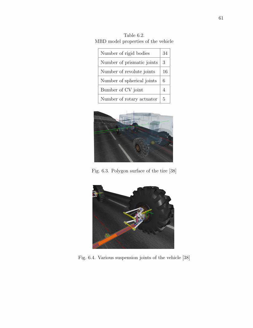
61

Table 6.2.MBD model properties of the vehicle



Number of revolute joints 16

Number of spherical joints 6

Bumber of CV joint 4

Number of rotary actuator 5

Fig. 6.3. Polygon surface of the tire [38]

Fig. 6.4. Various suspension joints of the vehicle [38]

62

Revolute joints are used to model most of the vehicle joints including [38]:

• Joints between the suspension control arms, knuckle, and frame.

• Joint between the wheel and knuckle.

• Joints between the axle and the frame.

• Joint between the drive shaft and the frame.

Fig. 6.5. MBD model of the entire vehicle chassis system [38]

63

7. CONCLUDING REMARKS AND FUTURE WORK

An explicit time integration multibody dynamics code was used to create a three-

dimensional multibody dynamics model of 3 experiments and a full vehicle simula-

tion, in order to calibrate a DEM soil model. The model has the following major

characteristics:

• A high fidelity multibody dynamics models are used for the experiments and

the full vehicle simulations.

• Particles geometric shape can be modeled using three types of shape represen-

tations: superquadric surface, assembly of spheres, and polygonal surface.

• A Cartesian Eulerian grid contact search algorithm is used to allow fast contact

detection between particles.

• Normal contact constraints are modeled using the penalty technique with a

penalty spring and an asymmetric damper.

• Friction is modeled using an asperity-based approximate Coulomb friction model.

• The rigid bodies rotational equations of motion are written in a body- xed

frame with the total rigid body rotation matrix updated each time step using

incremental rotations.

• The governing equations of motion are solved along with the contact constraint

equations using a time-accurate explicit solution procedure.

The soil model was used to validate experimental using cubical sand particles

Parametric studies were performed in order to study the effects of the particle size

and contact properties on the simulation results. The simulation results found to be

in very good co-relation with the experimental result.

64

Recommended Future Work

• Future work to be done to improve the correlation between experimental results

and simulation results by using a definite algorithm to tune contact properties.

• There is a necessity to perform further more soil experiments and validate the

DEM model using the experimental results to improve soil model fidelity by

increasing soil target properties like compressibility, bulk density, slope stability,

particle size.

• The edge effect of the soil particle container played a significant role in this

research and required many iterations to avoid such affects therefore work needs

to be done to identify correct sizing of the soil container which will eliminate

multiple iterations.

• Also, it is important to include cohesiveness of the soil and mixing multiple soils

in the simulation to represent accurately a real life heterogeneous soil.

• It is important to introduce flexible and pneumatic tires on the soft soil and

perform simulations to identify and caliberate tire parameters (tire pressure,

tread shapes etc.) to make it more efficient for vehicle application.

• Work needs to be done to validate full vehicle simulation results with proving

grounds results of a vehicle on a similar kind of soil.

REFERENCES

65

REFERENCES

[1] Wong, J. (2010). Terramechanics and Off-road Vehicle Engineering. Butterworth-Heinemann.

[2] Knight, S. (1961). ”Measuring Soil Trafficability Characteristics,”. NationalTechnical Information Service.

[3] Bekker, M. (1964). ”Mechanics of locomotion and lunar surface vehicle con-cepts,”.SAE Transactions.

[4] Bekker, M. (1960). ”Off-the-road locomotion,”. The University of MichiganPress, Ann Arbor, Michigan.

[5] Bekker, M. (1956). ”Theory of land locomotion,”. The University of MichiganPress, Ann Arbor, Michigan.

[6] Reece and Wong J. (1967). ”Prediction of rigid wheel performance based on theanalysis of soil-wheel stresses part I. Performance of driven rigid wheels,”. J.Terramechanics, vol. 4, p. 81–98.

[7] Reece and Wong J. (1967). ”Prediction of rigid wheel performance based on theanalysis of soil-wheel stresses part II. Performance of towed rigid wheels,”. J.Terramechanics, vol. 4, pp. 7-25.

[8] Fattah, R. N. Y. and E. A. (1976). ”Prediction of wheel-soil interaction andperformance using the finite element method,”. J. Terramechanics, vol. 13, no.4, p. 227–240.

[9] Knuth, M. A., Johnson, J.B., Hopkins, M. A., Sullivan, R. J. and Moore, J.M. (2011). ”Discrete element modeling of a Mars Exploration Rover wheel ingranular material,”. J. Terramechanics.

[10] Smith, W., Melanz, D., Senatore, C., Iagnemma, K. and Peng, H. (2013) ”Com-parison of DEM and traditional modeling methods for simulating steady-statewheel-terrain interaction for small vehicles”.

[11] Wong, C. and L. J.Y. (1996). ”Numerical simulations of tire-soil interactionbased on critical state soil mechanics,”. Journal of Terramechanics, vol. 33(5),pp. 209-221.

[12] Karafiath, L. (1984). ”Finite element analysis of ground deformation beneathmoving track loads,” . 8th International Conference of International society forTerrain-Vehicle Systems.

[13] Tsuji, T., Nakagawa, Y., Matsumoto, N., Kadono, Y., Takayama, T. and Tanaka,T. (2012). ”3-D DEM simulation of cohesive soil-pushing behavior by bulldozerblade,”. J. Terramechanics, vol. 49, p. 37–47.

66

[14] Cundall, P. (1971) ”A computer model for simulating progressive large-scalemovements in block rock mechanics,”. Proc. Symp. Int. Soc. Rock Mech. Nancy,vol. 2.

[15] Cundall, P. and Strack, O. (1979). ”A discrete numerical model for granularassemblies,”. Geotechnique, vol. 29, no. 1, pp. 47-65.

[16] Horner, D., Peters, J. and Carrillo, A. (1979). ”Large Scale Discrete ElementModeling of Vehicle-Soil Interaction,”. Journal of Engineering Mechanics, vol.127, pp. 1027-1032.

[17] Carrillo, A., Horner, D., Peters, J., and West, J. (1996). ”Design of a LargeScale Discrete Element Soil Model for High Performance Computing Systems,”.ACM/IEEE conference on Supercomputing.

[18] Drucker, D. C. and Prager, W. (1952). ”Soil mechanics and plastic analysis forlimit design,”. Quarterly of Applied Mathematics, vol. 10, no. 2, pp. 157-165.

[19] Youngs, D. (1987). ”An interface tracking method for a 3D Eulerian hydrody-namics code,”. Technical Report Atomic Weapons Research Establishment.

[20] Hirt, C. and Nichols, B. (1981). ”Volume of fluid (VOF) method for the dynamicsof free boundaries,”. Journal of Computational Physics, vol. 39, pp. 201-225.

[21] Wasfy, T., O’Kins, J. and Smith, S. (2008). ”Experimental Validation of a Time-Accurate Finite Element Model forCoupled Multibody Dynamics and LiquidSloshing,”. SAE 2007 Transactions, Journal of Passenger Cars: Mechanical Sys-tems, Vols. 2007-01-0139.

[22] Wasfy, T.M. (2004). ”Modeling spatial rigid multibody systems using an explicit-time,”. 28th Biennial Mechanisms and Robotics Conference, Salt Lake, Utah.

[23] Wasfy, T. (2003). ”Asperity spring friction model with application to belt-drives,”. DETC2003.

[24] Coetzee, C.J., Basson, A.H. and Vermeer, P. A. (2007). ”Discrete and continuummodeling,”. Journal of Terramechanics, vol. 44, pp. 177-186.

[25] Elperin, T. and Golshtein, E. (1997). ”Comparison of di,” Physica A, vol. 242,pp. 332-340.

[26] Advanced Science and Automation Corp. ”DIS :Dynamic Interactions Simula-tor,”. Retreived from http://www.ascience.com. [Accessed March 2013].

[27] Leamy, M. J. and Wasfy, T.M. (2002). ”Transient and steady-state dynamic,”,vol. 124, no. 4, pp. 575-581.

[28] Wasfy, T. (2015). ”Introduction to Hybrid-Electric Vehicle,”. IUPUI Course ME5970.

[29] Cundall, P.A. (1988). ”Formulation of a three-dimensional distinct element modelPart,”. International Journal of Rock Mechanics, Mining Science, vol. 25, no. 3,pp. 107-116.

67

[30] Ahmadi, S. G., Wasfy, T. M., Wasfy, H. M., and Peters, J. M. (2013). ”High-Fidelity modeling of a backhoe digging operation using an explicit multibodydynamics code with integrating discrete particle modeling capability,”. Publishedby ASME.

[31] Wasfy, T. M., Ahmadi, S. G., Wasfy, H. M. and Peters, J. M. (2013) ”MultibodyDynamic Modeling of Sand Flow from Hopper and Sand Pile Angle of Repose,”.ASME International Design Engineering Technical Conference.

[32] Wang, J. and Gutierrez, M. (2010). ”Discrete element simulations of direct shearspecimen scale effects”.

[33] Janosi, Z. and Hanamoto, B. (1961). ”The analytical determination of drawbarpull as a function of slip for tracked vehicles in deformable soils,”. 1st Interna-tional Conference on the Mechanics of Soil-Vehicle Systems, Torino, Italy.

[34] Janosi, Z. (1961). ”An analysis of pneumatic tire performance on deformablesoil,”. 1st International Conference on the Mechanics of Soil-Vehicle Systems,Troino, Italy.

[35] Melanza, D., Jayakumara P. and Negrut, D. (2015). ”Experimental Validationof a Differential Variational Inequality-Based Approach,” US Army RDECOM-TARDEC, Warren, Michigan.

[36] Senatore, C. (2014). ”Robotic Mobility Group; Laboratory for Manufacturingand Productivity; MIT,”. Cambridge, MA.

[37] Senatore, C., Wulfmeier, M., MacLennan, J., Jayakumar, P. and Iagnemma,K. (2012). ”Investigation of stress and failure in granular soils for lightweightrobotic vehicle application,”. NDIA Ground Vehicle Systems Engineering andTechnology Symposium, Michigan.

[38] Wasfy, T. M., Wasfy, H. M. and Peters, J. M. (2015). ”High-Fidelity MultibodyDynamics Vehicle Model Coupled with Cohesive Soil Discrete Element Model forpredicting Vehicle Mobility,”. ASME International Design Engineering TechnicalConference; 11th International Conference on Multibody Systems, NonlinearDynamics, and Control (MSNDC), Boston, MA, USA.

[39] Regli, G., Handke A. and Butikofer (1993). ”Material laws as a basis for simu-lation models for the calculation of wheelsoil interaction examination using thefinite element method,”. Journal of Terramechanics, vol. 30, no. 3, pp. 165-179.

[40] Shoop, S., Richmond. P. and Lacombe, J. (2006). ”Overview of cold regionsmobility modeling at CRREL,”. Journal of Terramechanics, vol. 43, no. 1, pp.1-26.

[41] Tekestea, M., Tollnera, E., Raperb, R., Wayb, T. and Johnson, C. (2009). ”Non-linear finite element analysis of cone penetration in layered sandy loam soil -Considering precompression stress state,”. Journal of Terramechanics, vol. 46,no. 5, pp. 229-239.

[42] Xia, K. (2011). ”Finite element modeling of tire/terrain interaction: Applicationto predicting soil compaction and tire mobility,”. Journal of Terramechanics, vol.48, no. 2, pp. 113-123.

Documents

EXPERIMENTAL VALIDATION OF NON-COHESIVE SOIL USING