EXPERIMENTAL STUDY ON DYNAMIC BEHAVIOUR OF TROPICAL RESIDUAL SOILS …eprints.utar.edu.my/2973/1/ESA-2018-1508242-1.pdf · 2018-08-06 · ii ABSTRACT EXPERIMENTAL STUDY ON DYNAMIC

EXPERIMENTAL STUDY ON DYNAMIC BEHAVIOUR OF TROPICAL RESIDUAL SOILS IN MALAYSIA

LIM JUN XIAN

MASTER OF ENGINEERING SCIENCE

LEE KONG CHIAN FACULTY OF ENGINEERING AND SCIENCE

UNIVERSITI TUNKU ABDUL RAHMAN FEBRUARY 2018

EXPERIMENTAL STUDY ON DYNAMIC BEHAVIOUR OF

TROPICAL RESIDUAL SOILS IN MALAYSIA

By

LIM JUN XIAN

A dissertation submitted to the Department of Civil Engineering,

Lee Kong Chian Faculty of Engineering and Science,

Universiti Tunku Abdul Rahman,

in partial fulfillment of the requirements for the degree of

Master of Engineering Science

February 2018

ii

ABSTRACT

EXPERIMENTAL STUDY ON DYNAMIC BEHAVIOUR OF

TROPICAL RESIDUAL SOILS IN MALAYSIA

Lim Jun Xian

In soil dynamics, most of the studies carried out abroad focused on

investigating the dynamic behaviours of pure sand and clay. Very limited

studies have been focused on the dynamic behaviours of tropical residual soil

in Malaysia. Although the 1g shaking table test can be used to investigate the

dynamic behaviours of soil, the accuracy of the integrated displacement data is

subjected to uncertainties. The present study aims to investigate the dynamic

properties (namely shear modulus and damping ratio) of two selected tropical

residual soils (i.e. sandy silt and sandy clay) and a sand mining trail in

Malaysia. Three different setups (i.e. large laminar shear box test, small

chamber test with positive air pressure, and small sample test with suction)

were tested on a 1g shaking table to evaluate the stress-strain relationship of

soils, and hence their secant shear modulus and damping ratios. The

experimental results were then compared with the established findings from

literature. The large laminar shear box test and small chamber test with

positive air pressure were capable of testing the dynamic properties of soils

covering for large (0.077 % - 1.48 %) and medium (0.017 % - 0.077 %) shear

strain amplitudes of soil deformation, respectively. The results from the small

sample test with suction were discarded owing to the noise effect and problem

iii

of data synchronization. The experimental shear moduli for sand mining trail

were found to agree well with the established degradation curves of sand. The

results of sand mining trail also could fit with the established curves of clay

owing to low plasticity index. However, the residual soils (sandy silt and

sandy clay) could not fit to the established degradation curves of sand and

clay. The damping ratios of the residual soils also deviated from the

established damping curves. It can be concluded that the studied topical

residual soils in Malaysia are unique and behave neither as pure sand nor clay.

Fine content was found to be one of the important parameters on the dynamic

properties of the studied tropical residual soils.

iv

ACKNOWLEDGEMENTS

I would like to express my gratitude to my research main supervisors, Ir. Dr.

Lee Min Lee and co-supervisor, Prof. Dr. Yasuo Tanaka. They are very

supportive and patience towards my research. Their continuous

encouragement and invaluable guidance have deepened my understanding on

all important aspects in academic study, ability of planning in research, and

beneficially enhance my personal development as well. Through the

progressive development, I manage to conduct experiments independently and

collaborate efficiently with the laboratory assistants. I would also like to thank

all the laboratory staffs in Universiti Tunku Abdul Rahman for their relentless

technical support in my research. Lastly, I would like to appreciate kindness of

my parents, brother and the enormous effort by all previous researchers.

Without the fruitful research works contributed by the previous scholars, my

research would not be achieved.

v

APPROVAL SHEET

This dissertation/thesis entitled “EXPERIMENTAL STUDY ON

DYNAMIC BEHAVIOUR OF TROPICAL RESIDUAL SOILS IN

MALASYIA” was prepared by LIM JUN XIAN and submitted as partial

fulfillment of the requirements for the degree of Master of Engineering

Science at Universiti Tunku Abdul Rahman.

Approved by:

___________________________

(Ir. Dr. Lee Min Lee) Date:…………………..

Associate Professor/Supervisor

Department of Civil Engineering

Faculty of Engineering Science

Universiti Tunku Abdul Rahman

___________________________

(Prof. Dr. Yasuo Tanaka) Date:…………………..

Professor/Co-Supervisor

Department of Civil Engineering

Faculty of Engineering Science

Universiti Tunku Abdul Rahman

vi

FACULTY OF ENGINEERING SCIENCE

UNIVERSITI TUNKU ABDUL RAHMAN

Date: __________________

SUBMISSION OF FINAL YEAR PROJECT /DISSERTATION/THESIS

It is hereby certified that LIM JUN XIAN (ID No: 15UEM08242) has completed

this dissertation/ thesis entitled “EXPERIMENTAL STUDY ON DYNAMIC

BEHAVIOUR OF TROPICAL RESIDUAL SOILS IN MALAYSIA” under the

supervision of Ir. Dr. Lee Min Lee (Supervisor) from the Department of Civil

Engineering, Faculty of Engineering Science , and Prof. Dr. Yasuo Tanaka (Co-

Supervisor) from the Department of Civil Engineering, Faculty of Engineering

Science.

I understand that University will upload softcopy of my dissertation/ thesis in pdf

format into UTAR Institutional Repository, which may be made accessible to

UTAR community and public.

Yours truly,

____________________

(LIM JUN XIAN)

vii

DECLARATION

I hereby declare that the dissertation is based on my original work except for

quotations and citations which have been duly acknowledged. I also declare

that it has not been previously or concurrently submitted for any other degree

at UTAR or other institutions.

Name ____________________________

Date _____________________________

viii

TABLE OF CONTENTS

Page

ABSTRACT ii

ACKNOWLEDGEMENTS iv

APPROVAL SHEET v

SUBMISSION SHEET vi

DECLARATION vii

LIST OF TABLES xi

LIST OF FIGURES xii

LIST OF SYMBOLS / ABBREVIATIONS xx

CHAPTER

1.0 INTRODUCTION 1

1.1 Background Study 1

1.2 Problem Statement 3

1.3 Aims and Objectives 4

1.4 Research Framework 5

1.5 Scope of Study 7

1.6 Structure of Thesis 7

2.0 LITERATURE REVIEW 10

2.1 Introduction 10

2.2 Seismic Activities in Malaysia 10

2.3 Tropical Residual Soils in Malaysia 12

2.4 Secant Shear Modulus and Damping Ratio 14

2.5 Shear Modulus Degradation Curves for Soils 16

2.5.1 Shear Modulus Degradation Curves

for Sandy Soils 18

2.5.2 Shear Modulus Degradation Curves for

Silt and Clay 22

2.6 Relationship between Damping Ratio and

Shear Strain Amplitude 25

2.7 Laboratory Study on Dynamic Behaviours of Soil 27

2.7.1 Hollow Cylinder Simple Shear Test 27

2.7.2 Cyclic Triaxial Test 31

2.7.3 Cyclic Direct Simple Shear Test 37

2.7.4 Shaking Table Test 40

2.8 Signal Processing 45

2.8.1 Earthquake Records 45

2.8.2 Baseline Correction 48

2.8.3 Digital Filtering 51

2.9 Concluding Remarks 54

3.0 METHODOLOGY 56

ix

3.1 Introduction 56

3.2 Soil Sampling and Physical Tests 56

3.2.1 Soil Sampling 56

3.2.2 Soil Physical Tests 58

3.3 Apparatus and Instrumentation 59

3.3.1 Shaking Table System 59

3.3.2 Accelerometer 63

3.3.3 Laser Displacement Sensor 64

3.3.4 Data Acquisition System 66

3.4 Calibration of Devices 67

3.4.1 Calibration of Shaking Table System 67

3.4.2 Calibration of Accelerometers 71

3.5 Setups of Testing Models 72

3.5.1 Large Laminar Shear Box Test (LLSBT) 72

3.5.2 Small Chamber Test with Positive

Air Pressure (SCT) 77

3.5.3 Small Sample Test with Suction (SSTS) 79

3.6 Testing Parameters 81


4.0 DATA PROCESSING 84

4.1 Introduction 84

4.2 Flowchart in Data Processing 84

4.3 Data Processing Methods 85


5.0 RESULT AND DISCUSSION 98

5.1 Introduction 98

5.2 Physical Properties of Soils 99

5.3 Analysis of Experimental Data 100

5.3.1 Analysis of Large Laminar Shear Box Test

(LLSBT) 100

5.3.2 Analysis of Small Chamber Test with

Positive Air Pressure (SCT) 110

5.3.3 Analysis of Small Sample Test with Suction

(SSTS) 112

5.3.4 Summarizing the Results of

Three Laboratory Setups 115

5.4 Dynamic Properties of Tropical Residual Soils 116

5.4.1 Relationships between Secant Shear Modulus and


5.4.2 Comparison of Present Data with

Previous Findings of Residual Soils 123

5.4.3 Effect of Plasticity Index and Confining Pressure

on Shear Modulus 127

5.4.4 Relationship between Damping Ratio and



x

6.0 CONCLUSION 139

6.1 Summary 139

6.2 Conclusions 139

6.3 Recommendation 142

REFERENCES 144

LIST OF PUBLICATION 148

xi

LIST OF TABLES

Table

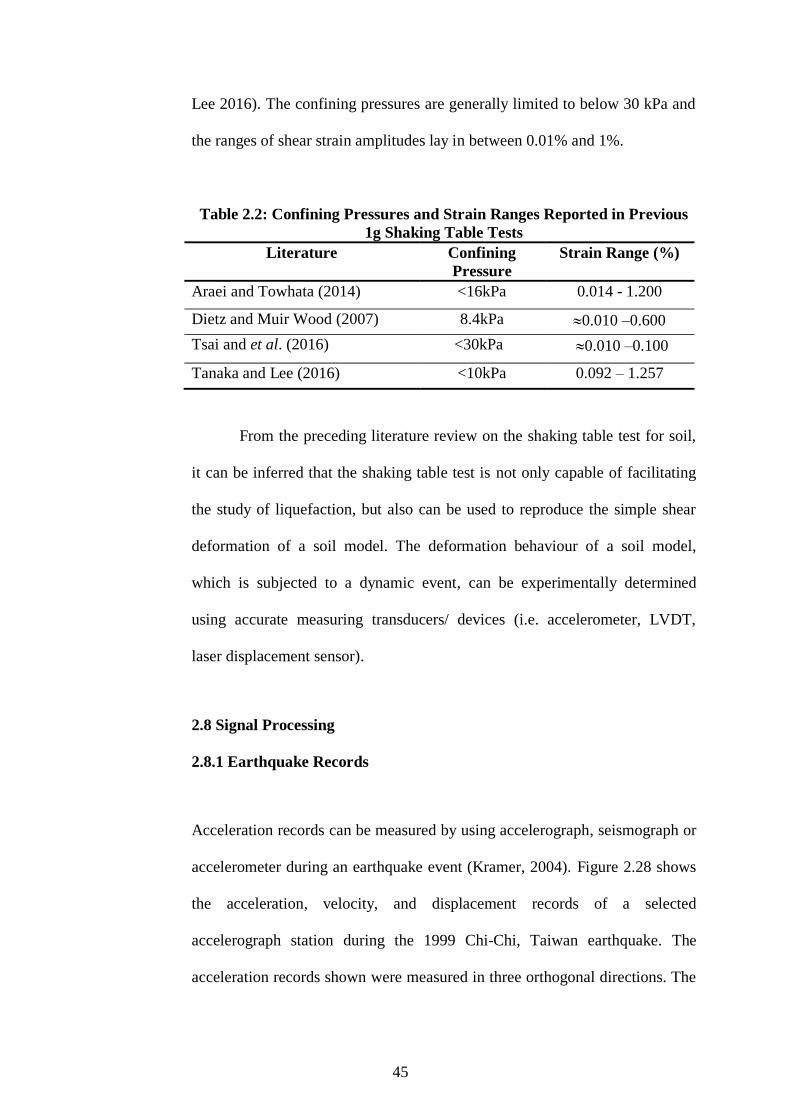
2.1

2.2

Constants for Equation 2.8

Confining Pressures and Strain Ranges Reported in

Previous 1g Shaking Table Tests

Page

30

45

3.1 Calibration of Accelerometers

72

3.2 Testing Parameters

82

3.3 Input Motions for Large Laminar Shear Box Test

82

3.4 Input Motions for Small Sample Tests

83

5.1 Physical Properties of Soils

99

5.2 Advantages and Shortcomings of the Three Setups

116

xii

LIST OF FIGURES

Figures

1.1

Research Framework

Page

6

2.1 Sumatran Faults and Subduction of the Indian-

Australian Plate into the Eurasian Plate (Balendra

et al., 2001)

11

2.2 Distribution of Tropical Residual Soils in Malaysia

(after Ooi, 1982)

14

2.3 Single-Cycle Hysteresis Loop (Brennan et al.,

2005)

15

2.4 Normalised Shear Modulus for Sandy Soil (after

Oztoprak and Bolton, 2013)

19

2.5 Hyperbolic Best-Fit Curves for Sandy Soils (after


20

2.6 Effect of Confining Pressure on Toyoura Sand

(after Oztoprak and Bolton, 2013)

21

2.7 Effect of Confining Pressure on Sand (Kokushu,

2004)

21

2.8 Normalised Shear Modulus Relationship for Silts

and Clays (Vardanega and Bolton, 2013)

23

2.9 Degradation Curves for Fine-grained Soils with

Static and Dynamic Adjustments (after Vardanega

and Bolton, 2013)

25

2.10 Influence of Vertical Effective Confining Pressure

on Damping Ratio of Saturated Sand (Seed and

Idriss, 1970)

26

2.11 Stress State of Hollow Cylinder Specimen (Xu et

al., 2013)

28

2.12 Relationship between Shear Modulus and Shear

Strain Amplitude for a Clean Dry Sand (Hardin

and Drnevich, 1972)

29

xiii

2.13 Degradation Curves for Dense Sand with different

Confining Pressures (Kokushu, 1980)

31

2.14 Degradation Curves for Dense Sand with different

Void Ratios (Kokushu, 1980)

32

2.15 Comparison of Singapore Jurong Formation Soils

and Degradation Curves by Seed and Idriss (1970)

(Leong et al., 2003)

33

2.16 Comparison of Singapore Jurong Formation Soils

and Piedmont Residual Soils (Leong et al., 2003)

34

2.17 Damping Ratio Relationship for Singapore

Residual Soils (Leong et al., 2003)

34

2.18 Best-Fit Stiffness Degradation Curves (Leong et

al., 2003)

35

2.19 Cyclic Triaxial Test Results for Singapore Tropical

Residual Soils (after Tou, 2003)

36

2.20 Comparison of Malaysia Tropical Residual Soil

and Singapore Residual Soils (Tanaka and Lee,

2016)

37

2.21 Stress Condition and Deformation in Direct

Simple Shear Test (Dyvik et al., 1987)

38

2.22 NGI Direct Simple Shear Device (Dyvik et al.,

1987)

38

2.23 Schematic Diagram of Double Specimens Direct

Simple Shear Device (Lanzo et al., 1997)

39

2.24 A Sample of Hysteresis Loop of Double

Specimens Direct Simple Shear Device (Lanzo et

al., 1997)

40

2.25 Shear Container in Shaking Table Test: (a)

Equivalent Shear Beam Container, (b) Laminar

Shear Box (after Dietz and Wood, 2007; Ueng et

al., 2007)

41

2.26 A Typical Hysteresis Loop of Soft Clay (Kazama

and Yanagisawa, 1996)

43

2.27 Acceleration and Displacement below Ground

Surface (Kazama et al., 1996)

43

xiv

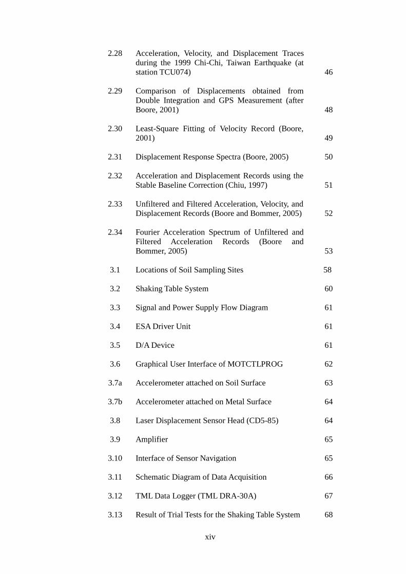
2.28 Acceleration, Velocity, and Displacement Traces

during the 1999 Chi-Chi, Taiwan Earthquake (at

station TCU074)

46

2.29 Comparison of Displacements obtained from

Double Integration and GPS Measurement (after

Boore, 2001)

48

2.30 Least-Square Fitting of Velocity Record (Boore,

2001)

49

2.31 Displacement Response Spectra (Boore, 2005) 50

2.32 Acceleration and Displacement Records using the

Stable Baseline Correction (Chiu, 1997)

51

2.33 Unfiltered and Filtered Acceleration, Velocity, and

Displacement Records (Boore and Bommer, 2005)

52

2.34 Fourier Acceleration Spectrum of Unfiltered and

Filtered Acceleration Records (Boore and

Bommer, 2005)

53

3.1 Locations of Soil Sampling Sites 58

3.2 Shaking Table System 60

3.3 Signal and Power Supply Flow Diagram 61

3.4 ESA Driver Unit 61

3.5 D/A Device 61

3.6 Graphical User Interface of MOTCTLPROG 62

3.7a Accelerometer attached on Soil Surface 63

3.7b Accelerometer attached on Metal Surface 64

3.8 Laser Displacement Sensor Head (CD5-85) 64

3.9 Amplifier 65

3.10 Interface of Sensor Navigation 65

3.11 Schematic Diagram of Data Acquisition 66

3.12 TML Data Logger (TML DRA-30A) 67

3.13 Result of Trial Tests for the Shaking Table System 68

xv

3.14 Relationships between Measured and Input

Frequencies

69

3.15 Relationships between Measured and Input

Displacements

70

3.16 Relationships between Peak Acceleration and

Input Displacement

71

3.17 Schematic Diagram of LLSBT 73

3.18 Experimental Setup for LLSBT 73

3.19 Sliding Joints on Aluminium Laminar Shear

Stacks

74

3.20 Aluminium Shear Box and Rubber Membrane 75

3.21 Compaction of Soil Layer 75

3.22 Soil Contained in Laminar Shear Box 76

3.23 Accelerometers in Soil Sample 77

3.24 Setup of SCT 78

3.25 Compacted Soil Sample 79

3.26 Schematic Diagram and Photograph of SSTS 80

4.1 Flowchart in Data Processing 85

4.2 Acceleration Profiles under Different Shaking

Frequencies

86

4.3 Velocity Profile 88

4.4 Displacement Profile 89

4.5 Displacement Waveforms of Shaking Table using

Laser Displacement Sensor

92

4.6 Fourier Amplitude Spectra of Actual Shaking

Table Displacement Movement

93

4.7 Comparison of Two Baseline Correction Schemes

and Laser Displacement Measurement (6Hz @ 2

mm)

94

xvi

4.8 Fourier Amplitude Spectra of Shaking Table

Record for the Motion of Laser Sensor Mounting

System, Ground Motion, Pre-event, and Post-event

Mean Motions (6Hz @ 2 mm)

96

5.1 Filtered Acceleration Profiles along the Height of

Soil Model

101-102

5.2 Filtered Displacement Profiles along the Height of

Soil Model

103-104

5.3 Displacement Profiles at Different Elevations 106

5.4 Comparison of Displacement Profiles between

Elevations of 3.5 cm and 10.5 cm

106

5.5 Shear Strain Profiles along Different Elevation

Intervals of Soil Model

107-108

5.6 Shear Stress Profile on the Top Surface at the

Elevation 10.5 cm

109

5.7 Hysteresis Loop for LLSBT 110

5.8 Shear Strain Profile for SCT 111

5.9 Shear Stress Profile for SCT 112

5.10 Hysteresis Loop for SCT 112

5.11 Shear Strain Profile for SSTS 113

5.12 Shear Stress Profile for SSTS 114

5.13 Hysteresis Loop for SSTS 115

5.14 Degradation Curves for Soil A (Sandy Clay) 119

5.15 Degradation Curves for Soil B (Sandy Silt) 120

5.16 Degradation Curves for Soil C (Silty Sand) 122

5.17 Results of Shear Modulus for Various Types of

Residual Soil

125

5.18 Effect of Confining Pressure on Shear Modulus for

Sandy Soil (Oztoprak and Bolton, 2013)

127

5.19 Effect of Plasticity Index on Shear Modulus for

Clayey Soil (Vardanega and Bolton, 2013)

128

xvii

5.20 Effect of Plasticity Index on Shear Modulus for

Soil A and Soil B

129

5.21 Effect of Confining Pressure on Shear Modulus

(Soil C)

130


(Soil A)

131


(Soil B)

132

5.24 Relationship between Damping Ratio and Shear

Strain Amplitude in LLSBT

135


Strain Amplitude in SCT

135


Strain Amplitude for Saturated Sand (Brennan et

al., 2005)

136

xx

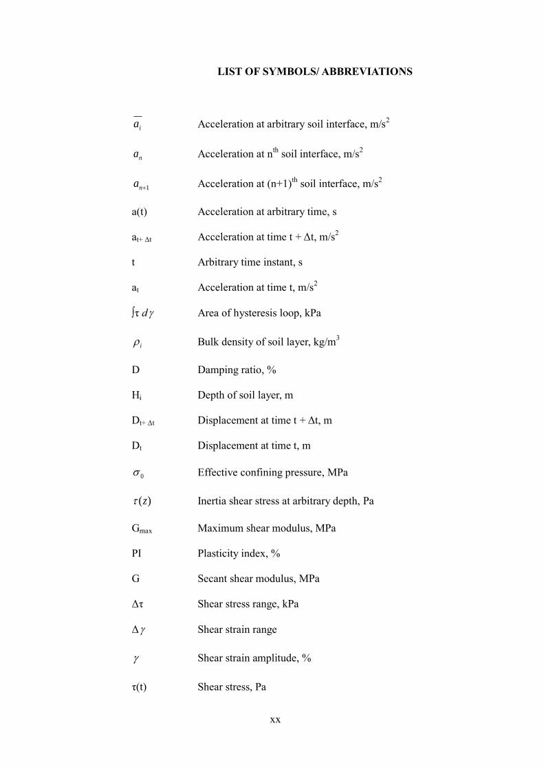
LIST OF SYMBOLS/ ABBREVIATIONS

ia Acceleration at arbitrary soil interface, m/s2

na Acceleration at nth

soil interface, m/s2

1na Acceleration at (n+1)th

soil interface, m/s2

a(t) Acceleration at arbitrary time, s

at+ Δt Acceleration at time t + Δt, m/s2

t Arbitrary time instant, s

at Acceleration at time t, m/s2

∫τ d Area of hysteresis loop, kPa

i Bulk density of soil layer, kg/m3

D Damping ratio, %

Hi Depth of soil layer, m

Dt+ Δt Displacement at time t + Δt, m

Dt Displacement at time t, m

0 Effective confining pressure, MPa

)(z Inertia shear stress at arbitrary depth, Pa

Gmax Maximum shear modulus, MPa

PI Plasticity index, %

G Secant shear modulus, MPa

Δτ Shear stress range, kPa

Δ Shear strain range

Shear strain amplitude, %

τ(t) Shear stress, Pa

xxi

Δt Time interval, s

e Void ratio

vt+ Δt Velocity at time t + Δt, m/s

vt Velocity at time t, m/s

GUI Graphical user interface

D/A Digital-to-analog

FAS Fourier amplitude spectrum

JF Jurong formation

LLSBT Large laminar shear box test

1g Single gravitational

SCT Small sample test with positive air pressure

SSTS Small sample test with suction

CHAPTER 1

INTRODUCTION

1.1 Background Study

Peninsular Malaysia is seismically affected by the far-field tremors and

earthquakes from neighbouring countries like Indonesia and Philippines. Some

of the notable earthquake incidents in the Southeast Asia region include the

2004 Aceh earthquake, the 2005 Nias earthquake, the 2000 Bengkulu

earthquake, the 2015 Sabah earthquake, etc. (Balendra, 2008). The

occurrences of seismic activities in Malaysia have attracted an increasing

attention from the public and authorities. Many studies pertaining to the

impact of earthquake focused on structural stability of buildings through

experimental testing or numerical simulation (Adnan and Suradi, 2008; Nazri

and Alexander, 2012). Studies on the soil dynamic and geotechnical

earthquake engineering are still very limited in Malaysia. This area of research

needs to be carried out progressively to enrich the database of dynamic

properties of soils in Malaysia.

In general, soil can be grouped into transported soil and residual soil.

The formation of soils largely depends on the topography, climate, and nature

of the parent rock. Residual soils are formed from rock (i.e. igneous,

metamorphic, and sedimentary) or accumulation of organic material and

2

remain at the place where they are formed (Huat et al., 2004). Malaysia, being

a tropical country with warm and humid climates, has abundant tropical

residual soils which are formed through intense physical and chemical

weathering processes. Intense rainfall, high humidity and temperature have

contributed to a thick residual soil deposit in the country (Huat et al., 2004).

Their physical properties are prominent criteria to be considered by engineers

during the design and planning stages of various engineering construction

works.

Extensive studies on the hydraulic properties, compressibility,

stiffness, and shear strength properties of residual soils can be easily traced

from the current available literature (Huat et al., 2004; Rahardjo et al., 2004;

Rahardjo et al., 2005). Several studies on dynamic behaviour of residual soils

have also been reported from different parts of the world (Borden et al., 1996;

Leong et al., 2003; Tanaka and Lee, 2016). However, studies on dynamic

behaviour of tropical residual soils in Malaysia are still very limited (Tanaka

and Lee, 2016).

Hardin and Black (1968) reported a number of factors that may

influence the shear modulus and damping ratio of soils. Those factors include

effective confining pressure (effective mean principal stress), void ratio,

degree of saturation, soil type, overconsolidation ratio, number of loading

cycles, shear strength parameters, and shear strain amplitude. The effects of

plasticity index and strain rate were found to be profound in fine-grained soils

(Vucetic and Dobry, 1991; Vardanega and Bolton, 2013). Statistical analyses

3

were carried out to form a relationship between shear modulus and shear strain

amplitude (Oztoprak and Bolton, 2013; Vardanega and Bolton, 2013). Various

types of soil dynamic laboratory tests can be used to investigate the dynamic

behaviour of soils. Among the tests include hollow cylinder simple shear test,

resonant column test, simple shear test, and shaking table test. Shaking table

test was widely used to investigate the problem of liquefaction and

deformation behaviour of soil models under a series of predesignated cyclic

motions (Kazama et al., 1996; Kazama and Yanagisawa, 1996).

Signal processing is required to process the acceleration records from

an earthquake event or a dynamic test. Baseline correction and digital filtering

techniques are among the popular approaches adopted to remove the low and

high-frequency noises from an actual signal (Boore and Bommer, 2005).

However, the integrated displacement data from an accelerometer is subjected

to uncertainties during the numerical integration process. Therefore, a direct

displacement measurement technique can be attempted as a reference when

processing the measured acceleration records.

1.2 Problem Statement

Malaysia is seismically threatened by the far-field earthquakes from

neighbouring countries and the near-field earthquakes as a result of localised

internal faults. The transmission of seismic waves through ground to the

building can have adverse effects on the superstructures. However, studies on

the response of soil to the seismic action have not been well studied in

Malaysia.

4

Previous studies on soil dynamics focused primarily on sandy and

clayey materials. However, residual soils which are the products of intensive

in-situ weathering of parent rocks cover more than three-quarters of the land

area in Peninsular Malaysia (Taha et al., 2000). The dynamic behaviour of

these residual soils which are complicated by their sand-clay mixture and

unsaturated state has yet been explored.

In a shaking table test, accelerometers are normally used to measure

the change of acceleration over time. Under normal data processing practices,

the acceleration data is adjusted and numerically integrated to obtain the linear

displacement data. However, the accuracy and reliability of the computed

displacement data and the adopted adjustment technique often raise

arguments.

1.3 Aim and Objectives

The aim of the present research is to investigate the dynamic properties of

selected tropical residual soils in Malaysia. Three objectives are set to achieve

the research aim:

i. To evaluate the performance of three different laboratory setups on a

1g shaking table for soil dynamic testing.

ii. To recommend the most suitable method of signal processing for the

shaking table test performed in this particular study.

5

iii. To investigate the dynamic properties of selected residual soils in

Malaysia.

1.4 Research Framework

The main objectives of this study are to determine the dynamic properties of

selected tropical residual soils in Malaysia and to examine the performance of

three different 1g shaking table test setups in laboratory. The main reasons of

selecting the shaking table test to investigate the dynamic behaviour of

tropical residual soils in the present study include (1) the shaking table test is

capable of reproducing simple shear deformations of a soil model. The

mechanism, which produces mechanical energy from the base towards the soil model,

can facilitate the understanding of soil deformation behaviour under a close-to-actual

seismic action; (2) the shaking table apparatus is readily available in the

geotechnical laboratory of author’s institution. To achieve the objectives, three

stages of research activities were undertaken, i.e. background study stage,

experimental stage, and data analysis stage. A research framework is

systematically laid out in Figure 1.1. The framework outlines all important

components of the study.

In the background study stage, state-of-the-art researches with regard

to soil dynamics and tropical residual soils are reviewed. Research gaps are

identified by critically examining the existing literature. From the identified

research gaps, three research objectives are formulated.

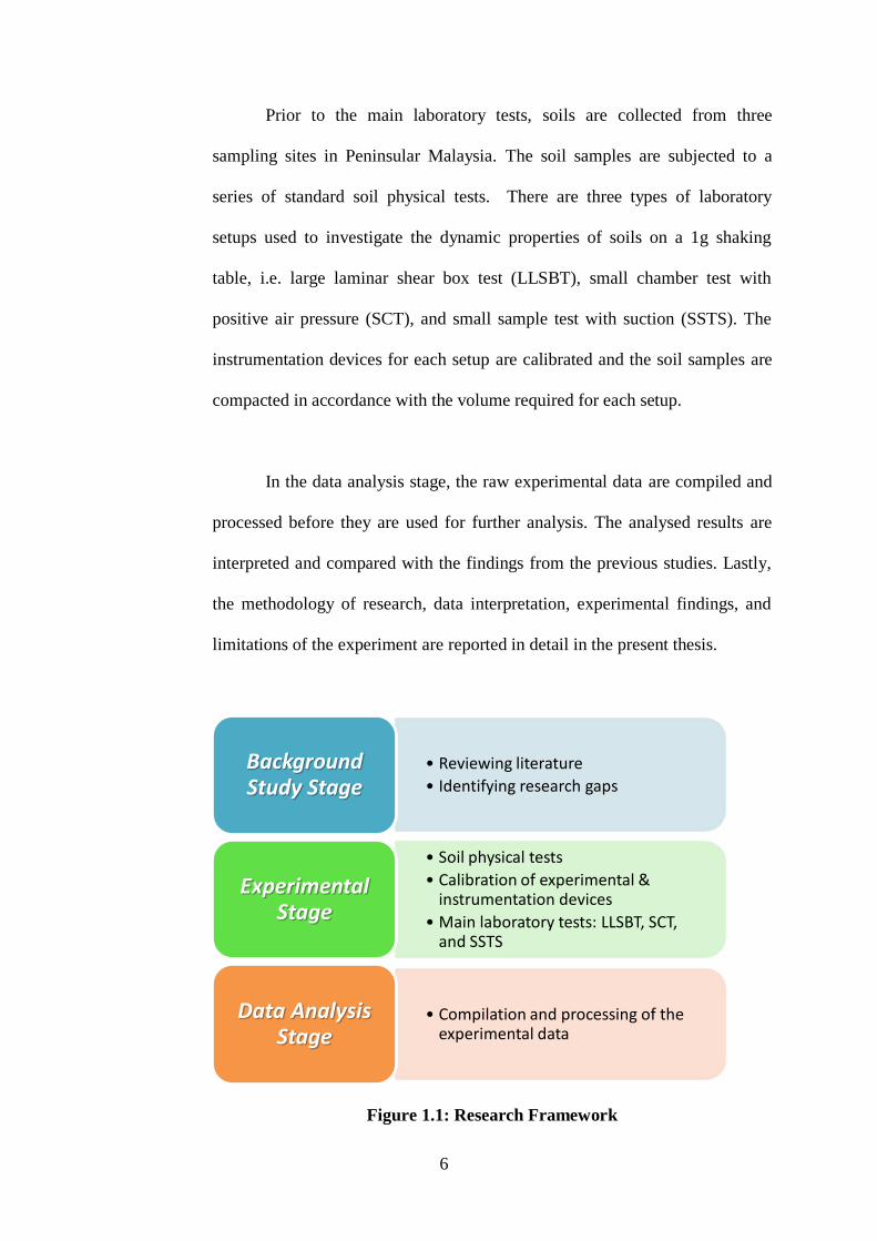
6

Prior to the main laboratory tests, soils are collected from three

sampling sites in Peninsular Malaysia. The soil samples are subjected to a

series of standard soil physical tests. There are three types of laboratory

setups used to investigate the dynamic properties of soils on a 1g shaking

table, i.e. large laminar shear box test (LLSBT), small chamber test with

positive air pressure (SCT), and small sample test with suction (SSTS). The

instrumentation devices for each setup are calibrated and the soil samples are

compacted in accordance with the volume required for each setup.

In the data analysis stage, the raw experimental data are compiled and

processed before they are used for further analysis. The analysed results are

interpreted and compared with the findings from the previous studies. Lastly,

the methodology of research, data interpretation, experimental findings, and

limitations of the experiment are reported in detail in the present thesis.

Figure 1.1: Research Framework

• Reviewing literature

• Identifying research gaps

Background Study Stage

• Soil physical tests

• Calibration of experimental & instrumentation devices

• Main laboratory tests: LLSBT, SCT, and SSTS

Experimental Stage

• Compilation and processing of the experimental data

Data Analysis Stage

7

1.5 Scope of Study

This study focuses on investigating the dynamic behaviours of selected soils in

Peninsular Malaysia using three different experimental setups tested on a 1g

shaking table. A sand mining trail (i.e. Silty Sand) and two selected tropical

residual soils (i.e. Sandy Clay and Sandy Silt) are adopted and tested on a 1g

shaking table by using three laboratory setups, namely large laminar shear box

test (LLSBT), small chamber test with positive air pressure (SCT), and small

sample test with suction (SSTS). The present experimental setups can

facilitate studies of medium-large shear strain dynamic properties of soil only.

Investigation of small-strain dynamic properties is not feasible owing to the

limitation of the laboratory setups. Each of the soil models is instrumented

with accelerometers for acceleration measurement and laser displacement

sensor for verification purposes. The dynamic properties of the soil are

interpreted from the experimental data and compared with the established

results from literature.

1.6 Structure of Thesis

This thesis is divided into six main chapters: Introduction (Chapter 1),

Literature Review (Chapter 2), Methodology (Chapter 3), Data Processing

(Chapter 4), Result and Discussion (Chapter 5), and Conclusion and

Recommendation (Chapter 6). Introductory note and concluding remark are

provided in each chapter to highlight the importance as well as to summarize

the chapter systematically.

8

Chapter 1 introduces the background study pertaining to the present

research. Problem statement, research aims, and objectives are clearly

formulated. Last but not least, the scope and limitation of the study is outlined.

Chapter 2 provides a literature review on the topics relevant to the

present research. This chapter begins with the formation and characteristics of

tropical residual soils as well as the occurrence of earthquakes in Malaysia.

Subsequently, studies of experimental soil dynamic behaviour reported by

numerous authors are critically reviewed.

Chapter 3 highlights the methodology of the three main laboratory

setups tested on a 1g shaking table, namely large laminar shear box test

(LLSBT), small chamber test with positive air pressure (SCT), and small

sample test with suction (SSTS). The physical properties of sampled soils and

preparation of the soil sample in each test are described in detail. In addition,

data acquisition system and calibration of instrumentation devices are

included.

Chapter 4 describes different approaches of data processing used to

process the measured acceleration data. Baseline correction and digital

filtering methods are used to recover the signal from low-frequency and high-

frequency noises. The acceleration data is adjusted and numerically integrated

to obtain corrected acceleration, velocity, and displacement data. A laser

displacement sensor is used as a reference when selecting an appropriate data

processing method in this particular study.

9

Chapter 5 discusses the results and findings obtained from the

experiments. The results of shear moduli and damping ratio of the three

selected soils are presented. Experimental data points are compared with the

established relationships reported from the established literature. Besides, the

influencing parameters of the soil dynamic properties are examined in detail.

Chapter 6 presents the conclusions drawn from the present study and

provides a list of recommendations for further improvement.

CHAPTER 2

LITERATURE REVIEW

2.1 Introduction

This chapter provides a review on the dynamic behaviour of soils (i.e. sand

and clay) obtained from different laboratory testing setups. Factors affecting

dynamic properties of soil are reported. The characteristics of tropical residual

soils and the occurrence of earthquakes in Malaysia are reviewed. In addition,

important aspects of signal processing and ground motion parameters are

studied.

2.2 Seismic Activities in Malaysia

Malaysia is situated on the southern edge of the Eurasian plate which is in the

vicinity of two active plate boundaries, namely the inter-plate boundary

between Indo-Australian and Eurasian plates as well as the inter-plate

boundary between Eurasian and Philippine plates (Mohd Rosaidi, 2001).

Figure 2.1 shows the Sumatran faults and subduction zone of the Indian-

Australian plate into Eurasian plate. Peninsular Malaysia (west part of

Malaysia) is located at the seismically stable part of the Eurasian plate while

East Malaysia is located at the moderately active zone (Balendra and Li, 2008;

Mohd Rosaidi, 2001).

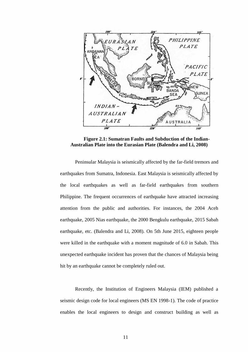
11

Figure 2.1: Sumatran Faults and Subduction of the Indian-

Australian Plate into the Eurasian Plate (Balendra and Li, 2008)

Peninsular Malaysia is seismically affected by the far-field tremors and

earthquakes from Sumatra, Indonesia. East Malaysia is seismically affected by

the local earthquakes as well as far-field earthquakes from southern

Philippine. The frequent occurrences of earthquake have attracted increasing

attention from the public and authorities. For instances, the 2004 Aceh

earthquake, 2005 Nias earthquake, the 2000 Bengkulu earthquake, 2015 Sabah

earthquake, etc. (Balendra and Li, 2008). On 5th June 2015, eighteen people

were killed in the earthquake with a moment magnitude of 6.0 in Sabah. This

unexpected earthquake incident has proven that the chances of Malaysia being

hit by an earthquake cannot be completely ruled out.

Recently, the Institution of Engineers Malaysia (IEM) published a

seismic design code for local engineers (MS EN 1998-1). The code of practice

enables the local engineers to design and construct building as well as

12

geotechnical structures with an adequate earthquake resistance. Besides, many

researchers from different fields have contributed to earthquake engineering in

many facets, such as seismology, structural engineering, geotechnical

earthquake engineering, etc. (Mohd Rosaidi, 2001; Shakri and Sanjery, 2015;

Sooria et al., 2012; Tanaka and Lee, 2016). Despite of the significant emphasis

put on earthquake engineering, the dynamic behaviour of soil in Malaysia still

has yet been well explored. Very limited studies have been carried out on the

geotechnical and earthquake engineering.

2.3 Tropical Residual Soils in Malaysia

In general, soil is an unconsolidated natural material and can be grouped into

transported soil and residual soil. The formation of soils largely depends on

the topography, climate, and nature of parent rock (Huat et al., 2004). Residual

soils are formed from rock (i.e. igneous, metamorphic, and sedimentary) or

accumulation of organic material and remain at the place where they were

formed (McCarthy, 1993). In addition, the Public Works Institute of Malaysia

(1996) defines a tropical residual soil as a soil formed by the decomposition of

parent material and remains in situ under tropical weathering conditions (i.e.

high temperature and humidity). Residual soils are composed of sand-to-clay

mixture with varying percentages of fine content. Over the passage of time,

the coarse-grained soil particles (e.g. quartz) will be weathered and become

clay-sized particles gradually. Unsaturated residual soils are considerably

complex attributed to several reasons, namely the behaviours of unsaturated

soils are wildly different as the air content in the void changes, the strength of

unsaturated soils cannot be described by the effective stress strength or

13

undrained shear strength, the volume will change in undrained condition when

conducting a triaxial test, and so on (Atkinson, 2007).

Residual soils originated from various types of parent rocks can be

found in many countries, particularly in the tropical regions, such as Malaysia,

Singapore, South Africa, Ghana, and Nigeria. Malaysia is a tropical country

with warm and humid climates and has abundant tropical residual soils as the

products of physical and chemical weathering processes. High rainfall,

humidity, and temperature give rise to a thick residual soil deposit in which

the rate of weathering is higher than the regions with cold and dry climates

(Huat et al., 2004). Ooi (1982) reported a geological map (referred to Figure

2.2) for the distribution of soils in Peninsular Malaysia in which the residual

soils in Malaysia can be categorized into three types based on their parent rock

formations (i.e. igneous rock, sedimentary rock, and metamorphic rock).

14

Figure 2.2: Distribution of Tropical Residual Soils in Malaysia (after Ooi,

1982)

2.4 Secant Shear Modulus and Damping Ratio

Secant shear modulus (G) and damping ratio (D) are two important dynamic

properties of soil for understanding deformation behaviour of soil under cyclic

loadings and for carrying out dynamic analysis of geotechnical structures

(Kramer, 2013). Both of the parameters can be evaluated from a representative

hysteresis loop as shown in Figure 2.3. Brennan et al. (2005) reviewed the

approaches to compute secant shear modulus and damping ratio. By definition,

secant shear modulus within a cycle of hysteresis loop is the ratio of the shear

stress range to the shear strain range. The range of shear stress (shear strain) is

15

defined by the difference between the maximum shear stress (shear strain

amplitude) and the minimum shear stress (shear strain amplitude) within the

representative hysteresis loop. As shown in Figure 2.3, the stiffness of soil is

defined by a representative slope in a single-cycle hysteresis loop. Eq (2.1)

shows the formula to compute the secant shear modulus.

G (2.1)

where

G = secant shear modulus, MPa

Δτ = shear stress range, MPa

Δ = shear strain range

Figure 2.3: Single-Cycle Hysteresis Loop (Brennan et al., 2005)

Eq (2.2) shows the formula to compute damping ratio in a hysteresis

loop. Damping ratio is proportional to the enclosed area of a hysteresis loop

16

and the area of the loop can be calculated by using trapezoidal integration

method.

)25.0(2

1

dD (2.2)

where

D = damping ratio

Δτ = shear stress range, kPa

Δ = shear strain range

∫τ d = area of hysteresis loop, kPa

2.5 Shear Modulus Degradation Curves for Soils

Hardin and Black (1968) identified a number of factors that may influence the

shear modulus and damping ratio of soils. These factors included effective

confining pressure (effective mean principal stress), void ratio, degree of

saturation, soil type, overconsolidation ratio, number of loading cycles, shear

strength parameters, and shear strain amplitude. Besides, the effects of

plasticity index and strain rate were found to be profound in fine-grained soils

(Vucetic and Dobry, 1991; Vardanega and Bolton, 2013). Lanzo et al. (1997)

investigated the effects of some parameters on the dynamic behaviours of sand

and clay by using a double specimen direct simple shear (DSDSS) device.

Among the parameters were soil types, vertical effective consolidation stress,

overconsolidation ratio, void ratio, shear strain amplitude, and plasticity index.

17

Deformation properties of soils (i.e. stiffness) are characterized by

using degradation curves in which the relationships between shear modulus

and shear strain amplitude are formed. Degradation curves of soils ranging

from small, medium to large shear strain amplitudes have been investigated in

numerous studies (Hardin and Drnevich, 1972; Oztoprak and Bolton, 2013;

Vardanega and Bolton, 2013; Ishibashi and Zhang, 1993; Kokushu, 1980;

Seed and Idriss, 1970). The responses of soils at very small shear strain level

(as small as 0.001 %) are important for conducting vibration analysis on a

geotechnical structure and understanding the mechanism of wave propagation

through a soil mass. Dynamic properties covering a wide range of shear strain

amplitudes have to be determined to facilitate the study of soil behaviour in an

earthquake (Hardin and Drnevich, 1972).

Since Seed and Idriss (1970) published the first database of shear

modulus degradation curves for sand, many researches have suggested

numerous degradation curves covering a wide variety of soils. Recently, a

newly-developed database of shear modulus degradation curves for sandy as

well as clayey soils have been reported by some researchers (Oztoprak and

Bolton, 2013; Vardanega and Bolton, 2013). The construction of shear

modulus degradation curves involved statistical analysis on the database of

shear moduli from many tests published previously. It follows that the above-

mentioned database of degradation curves are suitable to be used to compare

with the laboratory results in the present study.

18

2.5.1 Shear Modulus Degradation Curves for Sandy Soils

Figure 2.4 shows the shear modulus degradation curves for sandy soils

reported by Oztoprak and Bolton (2013). From the degradation curves, the

shear moduli attenuated with the increase of shear strain amplitudes. The

stiffness of soil (i.e. normalised secant shear modulus) was strain-dependant

and behaved non-linearly. The secant shear modulus at a very small shear

strain level gave rise to the maximum shear modulus (Gmax) in which linear

elastic behaviour of soil was expected. Hardin and Black (1968) reported an

empirical equation for computing the maximum shear modulus of coarse-

grained soils (Eq 2.3).

2

1

0

2

max1

)97.2(3230

e

eG

(2.3)

where

Gmax = maximum shear modulus, MPa

e = void ratio

0 = effective confining pressure, MPa

19

Figure 2.4: Normalised Shear Modulus for Sandy Soil (after Oztoprak

and Bolton, 2013)

Oztoprak and Bolton (2013) conducted a statistical analysis on the

database of shear modulus covering 454 tests from the previous studies. The

data were best fitted by formulating modified hyperbolic relationships. The

database covered a wide variety of granular soils including dry, wet, saturated,

reconstituted, and undisturbed samples of clean sands, gravels, sands with

fines and / or gravels, and gravels with sands and fines. Sixty nine types of

granular materials were used in the analysis including Toyoura sand, Ottawa

sand, undisturbed Ishikari sand, and etc. The granular materials used were

mostly sands of various grading, but mainly quite uniform, with some gravels.

The relative density was mostly high but with some looser samples. The

confinement pressures were mostly between 50 kPa and 600 kPa, with a

median of 150 kPa. Eq. 2.4 shows a formula developed by Oztoprak and

Bolton (2013) that can be used to predict the degradation curves for sandy

soils. From that, three hyperbolic curves (i.e. lower bound curve, mean curve,

and upper bound curve as shown in Figure 2.5) could be obtained for sandy

20

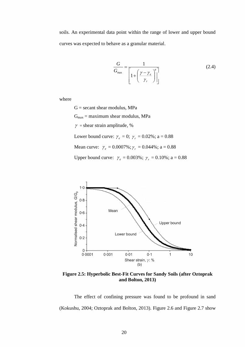
soils. An experimental data point within the range of lower and upper bound

curves was expected to behave as a granular material.

a

r

eG

G

1

1

max

(2.4)

where



= shear strain amplitude, %

Lower bound curve: e = 0; r = 0.02%; a = 0.88

Mean curve: e = 0.0007%; r = 0.044%; a = 0.88

Upper bound curve: e = 0.003%; r = 0.10%; a = 0.88

Figure 2.5: Hyperbolic Best-Fit Curves for Sandy Soils (after Oztoprak

and Bolton, 2013)

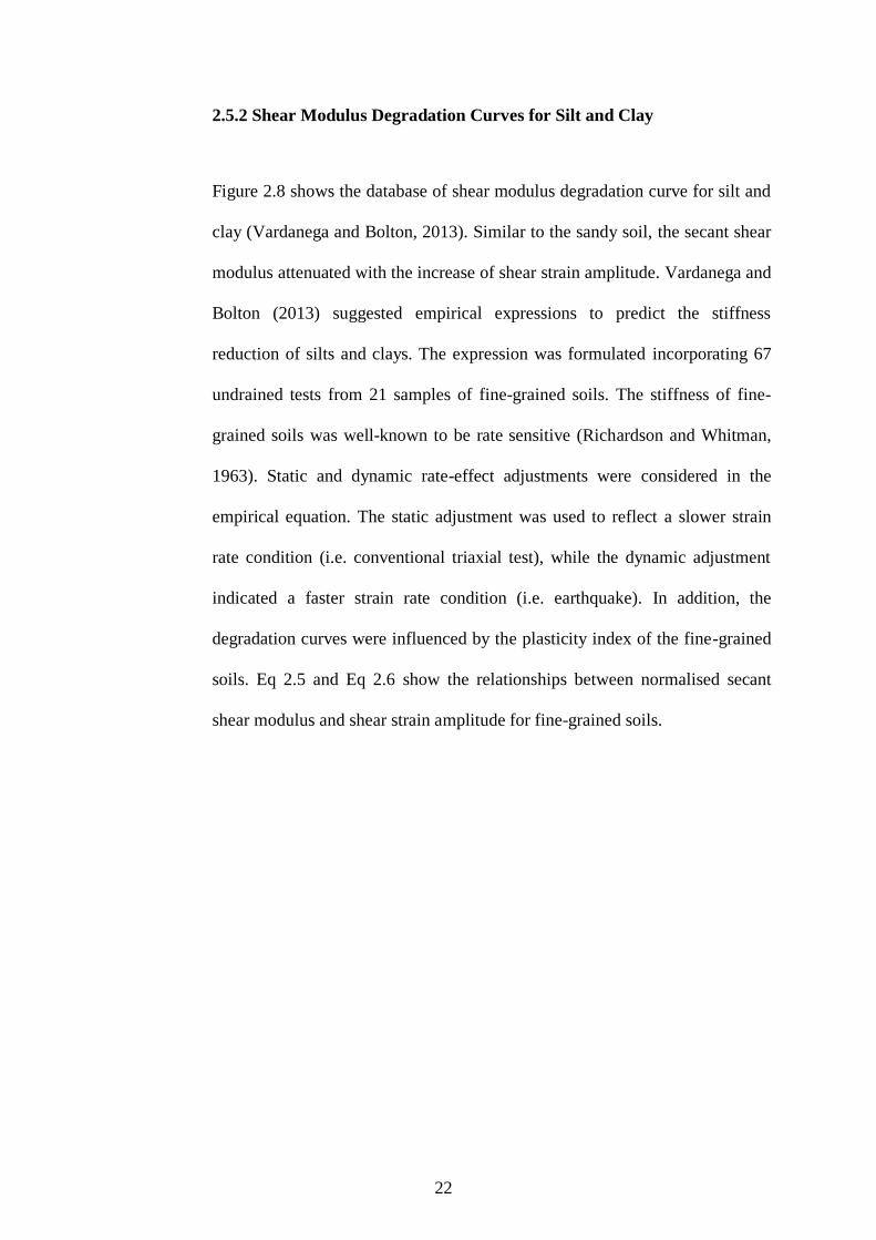
The effect of confining pressure was found to be profound in sand

(Kokushu, 2004; Oztoprak and Bolton, 2013). Figure 2.6 and Figure 2.7 show

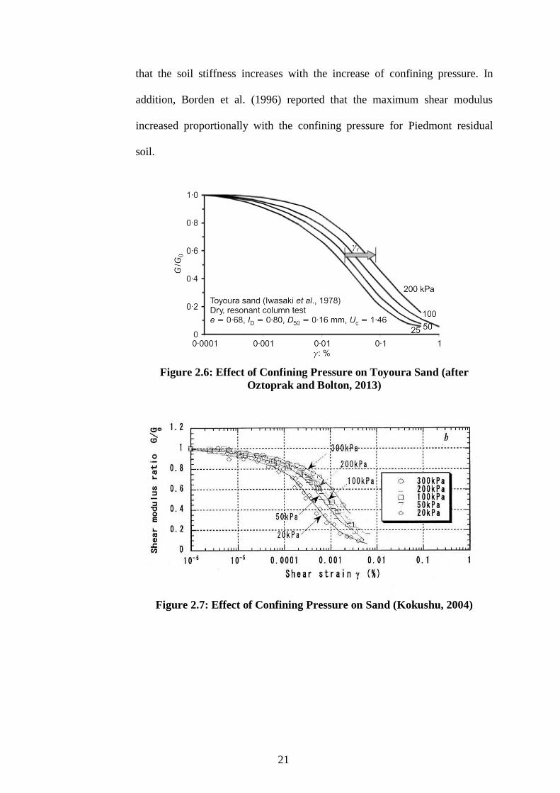
21

that the soil stiffness increases with the increase of confining pressure. In

addition, Borden et al. (1996) reported that the maximum shear modulus

increased proportionally with the confining pressure for Piedmont residual

soil.

Figure 2.6: Effect of Confining Pressure on Toyoura Sand (after


Figure 2.7: Effect of Confining Pressure on Sand (Kokushu, 2004)

22

2.5.2 Shear Modulus Degradation Curves for Silt and Clay

Figure 2.8 shows the database of shear modulus degradation curve for silt and

clay (Vardanega and Bolton, 2013). Similar to the sandy soil, the secant shear

modulus attenuated with the increase of shear strain amplitude. Vardanega and

Bolton (2013) suggested empirical expressions to predict the stiffness

reduction of silts and clays. The expression was formulated incorporating 67

undrained tests from 21 samples of fine-grained soils. The stiffness of fine-

grained soils was well-known to be rate sensitive (Richardson and Whitman,

1963). Static and dynamic rate-effect adjustments were considered in the

empirical equation. The static adjustment was used to reflect a slower strain

rate condition (i.e. conventional triaxial test), while the dynamic adjustment

indicated a faster strain rate condition (i.e. earthquake). In addition, the

degradation curves were influenced by the plasticity index of the fine-grained

soils. Eq 2.5 and Eq 2.6 show the relationships between normalised secant

shear modulus and shear strain amplitude for fine-grained soils.

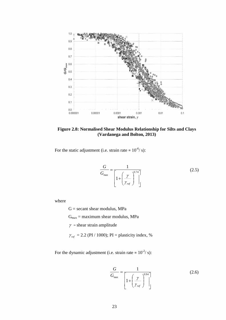
23

Figure 2.8: Normalised Shear Modulus Relationship for Silts and Clays

(Vardanega and Bolton, 2013)

For the static adjustment (i.e. strain rate = 10-6

/ s):

74.0

max

1

1

ref

G

G

(2.5)

where



= shear strain amplitude

ref = 2.2 (PI / 1000); PI = plasticity index, %

For the dynamic adjustment (i.e. strain rate = 10-2

/ s):

94.0

max

1

1

ref

G

G

(2.6)

24

where




ref = 3.7 (PI / 1000); PI = plasticity index, %

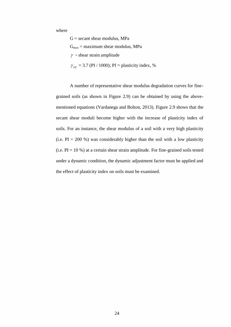
A number of representative shear modulus degradation curves for fine-

grained soils (as shown in Figure 2.9) can be obtained by using the above-

mentioned equations (Vardanega and Bolton, 2013). Figure 2.9 shows that the

secant shear moduli become higher with the increase of plasticity index of

soils. For an instance, the shear modulus of a soil with a very high plasticity

(i.e. PI = 200 %) was considerably higher than the soil with a low plasticity

(i.e. PI = 10 %) at a certain shear strain amplitude. For fine-grained soils tested

under a dynamic condition, the dynamic adjustment factor must be applied and

the effect of plasticity index on soils must be examined.

25

Figure 2.9: Degradation Curves for Fine-grained Soils with Static and

Dynamic Adjustments (Vardanega and Bolton, 2013)

2.6 Relationship between Damping Ratio and Shear Strain Amplitude

It is well accepted that damping ratio increases with the increase of shear

strain amplitude (Hardin and Drnevich, 1972; Ishibashi and Zhang, 1993; Seed

and Idriss, 1970). Figure 2.10 shows the relationship between damping ratio

and shear strain amplitude for a saturated sand (Seed and Idriss, 1970).

26

Besides, Hardin and Drnevich (1972) reported that vertical effective confining

pressure was the main factor influencing the damping ratio of sand. At a

certain shear strain amplitude, the damping ratio decreased as the confining

pressure increased. It was also found that void ratio and degree of saturation

were less influential on the damping ratio than the vertical effective pressure.

Figure 2.10: Influence of Vertical Effective Confining Pressure on

Damping Ratio of Saturated Sand (Seed and Idriss, 1970)

Hardin and Drnevich (1972) and Ishibashi and Zhang (1993) found

that damping ratio was a function of the normalised shear modulus (i.e. G/

Gmax). In addition, Ishibashi and Zhang (1993) provided a simple unified

formula relating shear modulus and damping ratio with the maximum shear

modulus, shear strain amplitude, mean effective confining stress, and plasticity

index. Eq 2.7 shows the simple relationship to formulate damping ratio curves

for a variety of soils.

27

1547.1586.02

)1(333.0

max

2

max

0145.0 3.1

G

G

G

GeD

PI

(2.7)

where

D = damping ratio, %

e = void ratio

PI = plasticity index, %



2.7 Laboratory Study on Dynamic Behaviour of Soil

There are various laboratory tests that can be used to investigate the dynamic

behaviours of soil, such as resonant column test, cyclic triaxial test, cyclic

direct simple shear test, cyclic torsional shear test, bender element test, and

shaking table test (Kramer, 2014). The dynamic properties measured by using

the above-mentioned tests are able to cover a wide range of shear strain

amplitudes. Seed and Idriss (1970) provided a list of approximate ranges of

shear strain amplitudes for laboratory tests and field tests, respectively.

2.7.1 Hollow Cylinder Simple Shear Test

Hollow cylinder simple shear device is normally used to investigate the soil

behaviours under shearing as well as the dynamic properties at a small strain

level (Hardin and Drnevich, 1972; Iwasaki et al., 1978; Wijewikreme and

Vaid, 2008). Figure 2.11 shows a schematic diagram of the stress condition of

soil in a hollow cylinder simple shear test (Xu et al., 2013). One of the

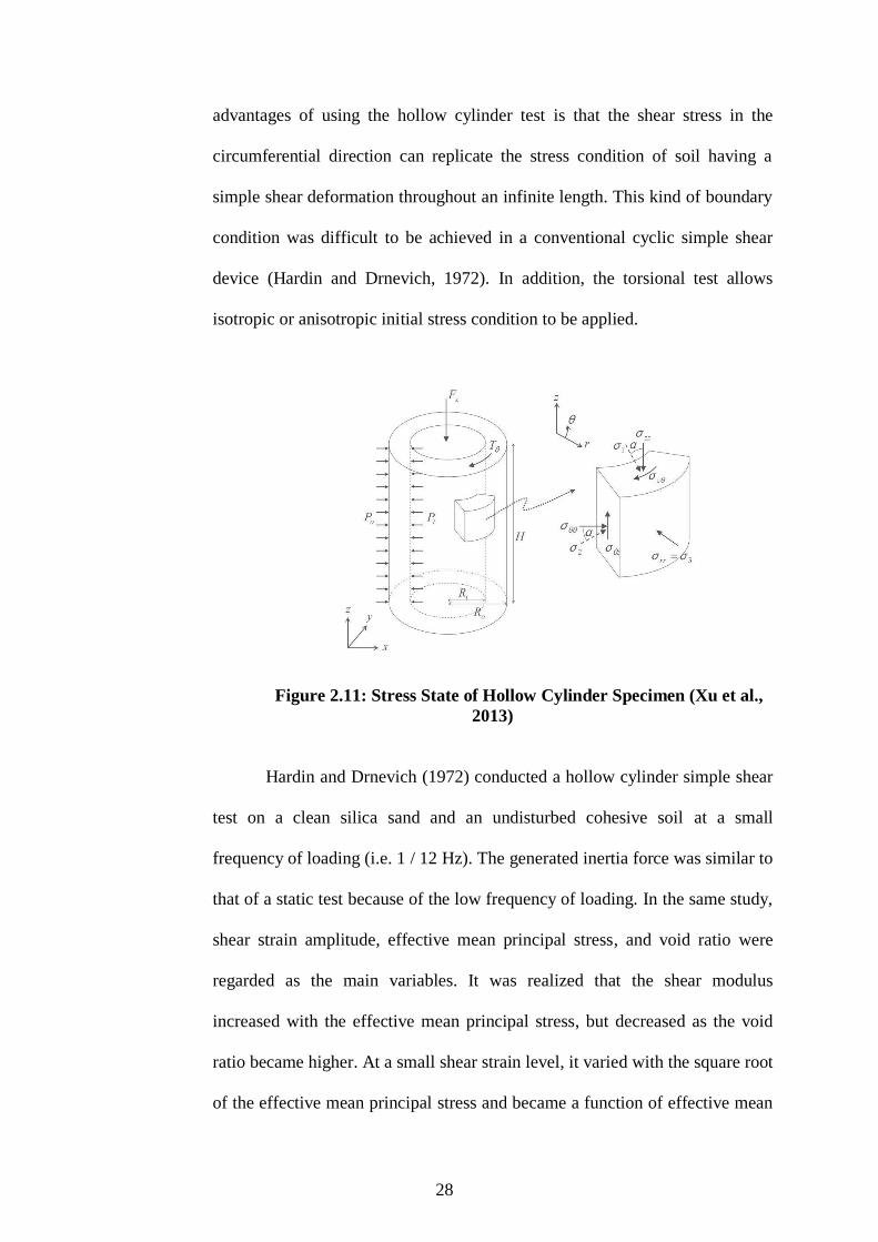
28

advantages of using the hollow cylinder test is that the shear stress in the

circumferential direction can replicate the stress condition of soil having a

simple shear deformation throughout an infinite length. This kind of boundary

condition was difficult to be achieved in a conventional cyclic simple shear

device (Hardin and Drnevich, 1972). In addition, the torsional test allows

isotropic or anisotropic initial stress condition to be applied.

Figure 2.11: Stress State of Hollow Cylinder Specimen (Xu et al.,

2013)

Hardin and Drnevich (1972) conducted a hollow cylinder simple shear

test on a clean silica sand and an undisturbed cohesive soil at a small

frequency of loading (i.e. 1 / 12 Hz). The generated inertia force was similar to

that of a static test because of the low frequency of loading. In the same study,

shear strain amplitude, effective mean principal stress, and void ratio were

regarded as the main variables. It was realized that the shear modulus

increased with the effective mean principal stress, but decreased as the void

ratio became higher. At a small shear strain level, it varied with the square root

of the effective mean principal stress and became a function of effective mean

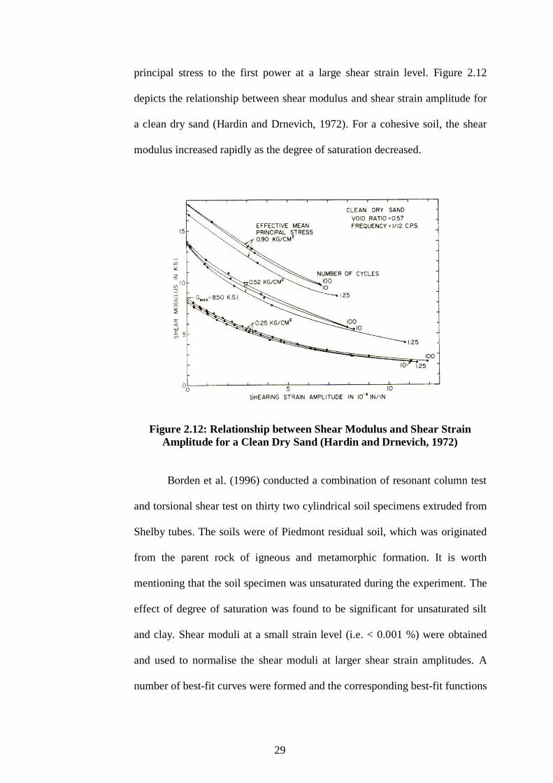
29

principal stress to the first power at a large shear strain level. Figure 2.12

depicts the relationship between shear modulus and shear strain amplitude for

a clean dry sand (Hardin and Drnevich, 1972). For a cohesive soil, the shear

modulus increased rapidly as the degree of saturation decreased.

Figure 2.12: Relationship between Shear Modulus and Shear Strain

Amplitude for a Clean Dry Sand (Hardin and Drnevich, 1972)

Borden et al. (1996) conducted a combination of resonant column test

and torsional shear test on thirty two cylindrical soil specimens extruded from

Shelby tubes. The soils were of Piedmont residual soil, which was originated

from the parent rock of igneous and metamorphic formation. It is worth

mentioning that the soil specimen was unsaturated during the experiment. The

effect of degree of saturation was found to be significant for unsaturated silt

and clay. Shear moduli at a small strain level (i.e. < 0.001 %) were obtained

and used to normalise the shear moduli at larger shear strain amplitudes. A

number of best-fit curves were formed and the corresponding best-fit functions

30

were formulated by using the normalised shear moduli. The effects of shear

strain amplitude, confining pressure, void ratio, and frequency of loading on

the soil dynamic properties were examined in detail. Eq 2.8 shows the formula

expressing the relationship between normalised shear modulus and shear strain

amplitude for the Piedmont residual soils.

cb

aG

G

1

1

max

(2.8)

where

G = shear modulus, MPa



a, b, c = constants depending upon the soil types, as shown in Table 2.1

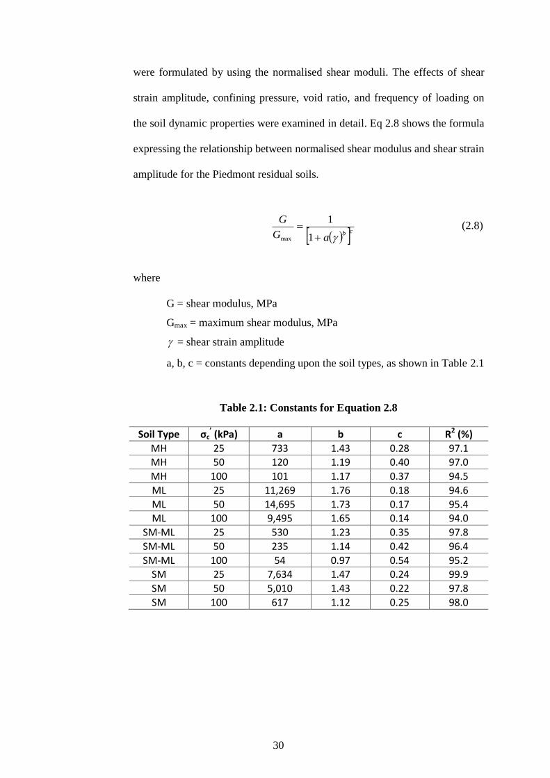
Table 2.1: Constants for Equation 2.8

Soil Type σc’ (kPa) a b c R2 (%)

MH 25 733 1.43 0.28 97.1 MH 50 120 1.19 0.40 97.0

MH 100 101 1.17 0.37 94.5

ML 25 11,269 1.76 0.18 94.6

ML 50 14,695 1.73 0.17 95.4

ML 100 9,495 1.65 0.14 94.0

SM-ML 25 530 1.23 0.35 97.8

SM-ML 50 235 1.14 0.42 96.4

SM-ML 100 54 0.97 0.54 95.2 SM 25 7,634 1.47 0.24 99.9

SM 50 5,010 1.43 0.22 97.8

SM 100 617 1.12 0.25 98.0

31

2.7.2 Cyclic Triaxial Test

Cyclic triaxial test has been widely used to investigate the dynamic behaviours

of various types of soils (Kokushu, 1980; Leong et al., 2003; Tanaka and Lee,

2016; Tou, 2003). Kokushu (1980) examined the effects of shear strain

amplitude, effective confining pressure, and void ratio on the dynamic

properties of saturated Toyoura sand extending to a very small strain range.

Figure 2.13 and Figure 2.14 show the degradation curves of the saturated

Toyoura sand, in which the effects of confining pressure and void ratio were

examined.

Figure 2.13: Degradation Curves for Dense Sand with different

Confining Pressures (Kokushu, 1980)

32

Figure 2.14: Degradation Curves for Dense Sand with different

Void Ratios (Kokushu, 1980)

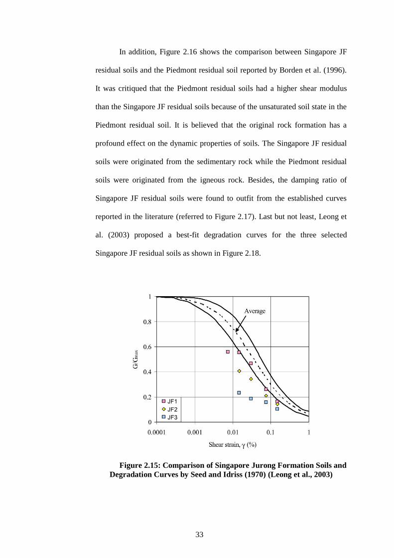
Leong et al. (2003) studied the dynamic behaviours of three selected

Singapore Jurong Formation tropical residual soils (denoted as JF1, JF2, and

JF3) by using a cyclic triaxial device tested with a loading frequency of 0.5

Hz. The fine contents of JF1, JF2, and JF3 were 75 %, 64 %, and 67 %,

respectively. In accordance with Unified Soil Classification System (USCS),

the JF1 was classified as a silt with low plasticity, while JF2 and JF3 were

classified as clay with low plasticity. The cyclic triaxial test was carried out

with an axial strain-controlled (0.005 % - 1 %) under an undrained condition.

Figure 2.15 shows the comparison of Singapore JF residual soils and the

degradation relationships established by Seed and Idriss (1970). The

experimental data of Singapore JF residual soils were scattered below the

established degradation curves. The shear moduli of JF3 soil was the lowest

among the three Singapore JF residual soils. It is noteworthy that the

maximum shear modulus was computed using the empirical equations

proposed by Hardin and Black (1968), as presented in Eq 2.3.

33

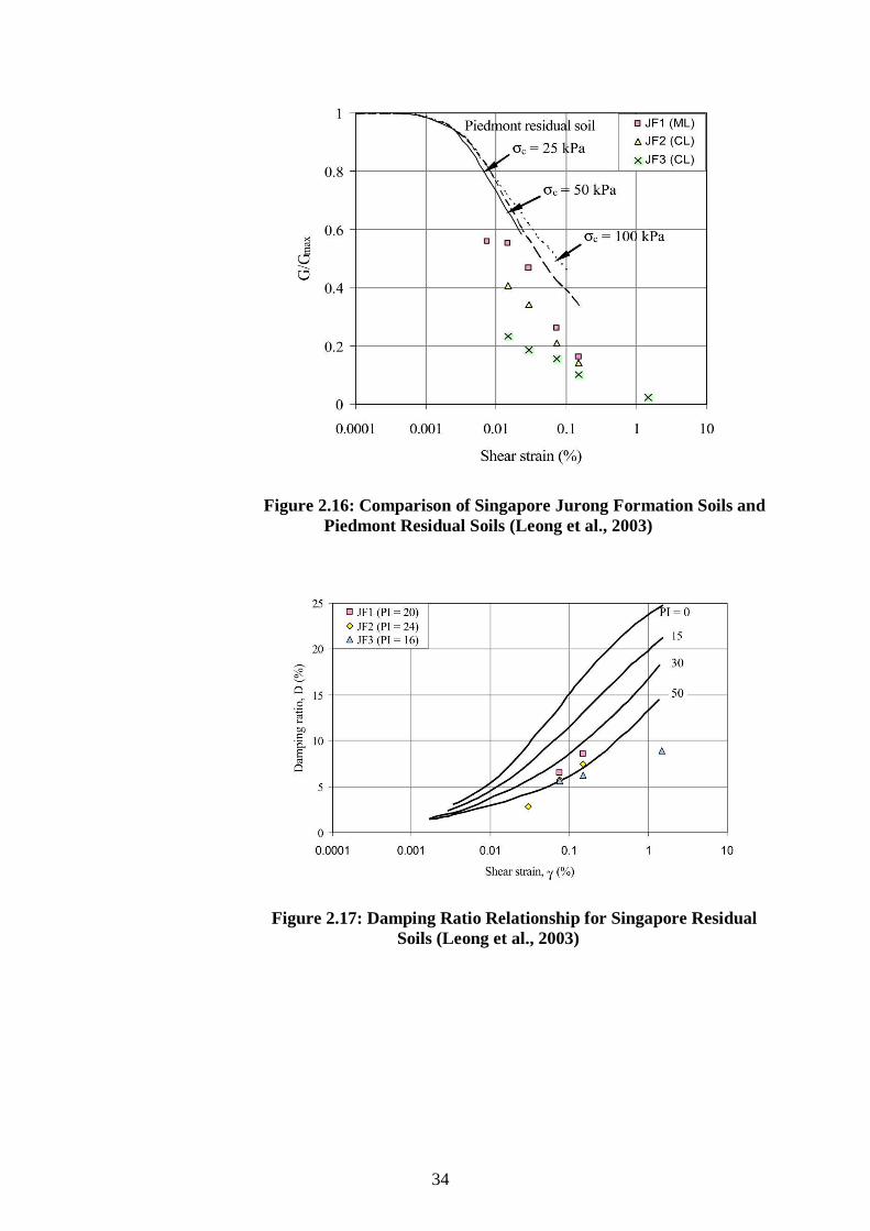
In addition, Figure 2.16 shows the comparison between Singapore JF

residual soils and the Piedmont residual soil reported by Borden et al. (1996).

It was critiqued that the Piedmont residual soils had a higher shear modulus

than the Singapore JF residual soils because of the unsaturated soil state in the

Piedmont residual soil. It is believed that the original rock formation has a

profound effect on the dynamic properties of soils. The Singapore JF residual

soils were originated from the sedimentary rock while the Piedmont residual

soils were originated from the igneous rock. Besides, the damping ratio of

Singapore JF residual soils were found to outfit from the established curves

reported in the literature (referred to Figure 2.17). Last but not least, Leong et

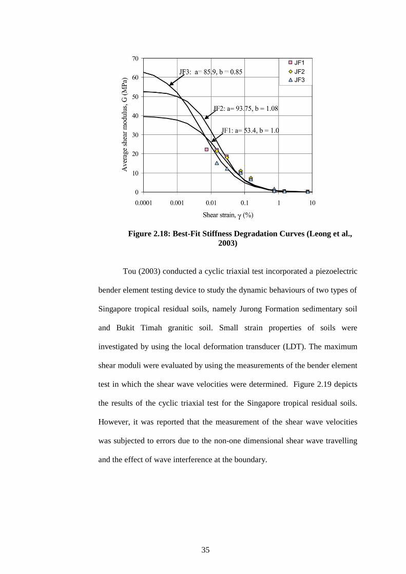
al. (2003) proposed a best-fit degradation curves for the three selected

Singapore JF residual soils as shown in Figure 2.18.

Figure 2.15: Comparison of Singapore Jurong Formation Soils and

Degradation Curves by Seed and Idriss (1970) (Leong et al., 2003)

34

Figure 2.16: Comparison of Singapore Jurong Formation Soils and

Piedmont Residual Soils (Leong et al., 2003)

Figure 2.17: Damping Ratio Relationship for Singapore Residual

Soils (Leong et al., 2003)

35

Figure 2.18: Best-Fit Stiffness Degradation Curves (Leong et al.,

2003)

Tou (2003) conducted a cyclic triaxial test incorporated a piezoelectric

bender element testing device to study the dynamic behaviours of two types of

Singapore tropical residual soils, namely Jurong Formation sedimentary soil

and Bukit Timah granitic soil. Small strain properties of soils were

investigated by using the local deformation transducer (LDT). The maximum

shear moduli were evaluated by using the measurements of the bender element

test in which the shear wave velocities were determined. Figure 2.19 depicts

the results of the cyclic triaxial test for the Singapore tropical residual soils.

However, it was reported that the measurement of the shear wave velocities

was subjected to errors due to the non-one dimensional shear wave travelling

and the effect of wave interference at the boundary.

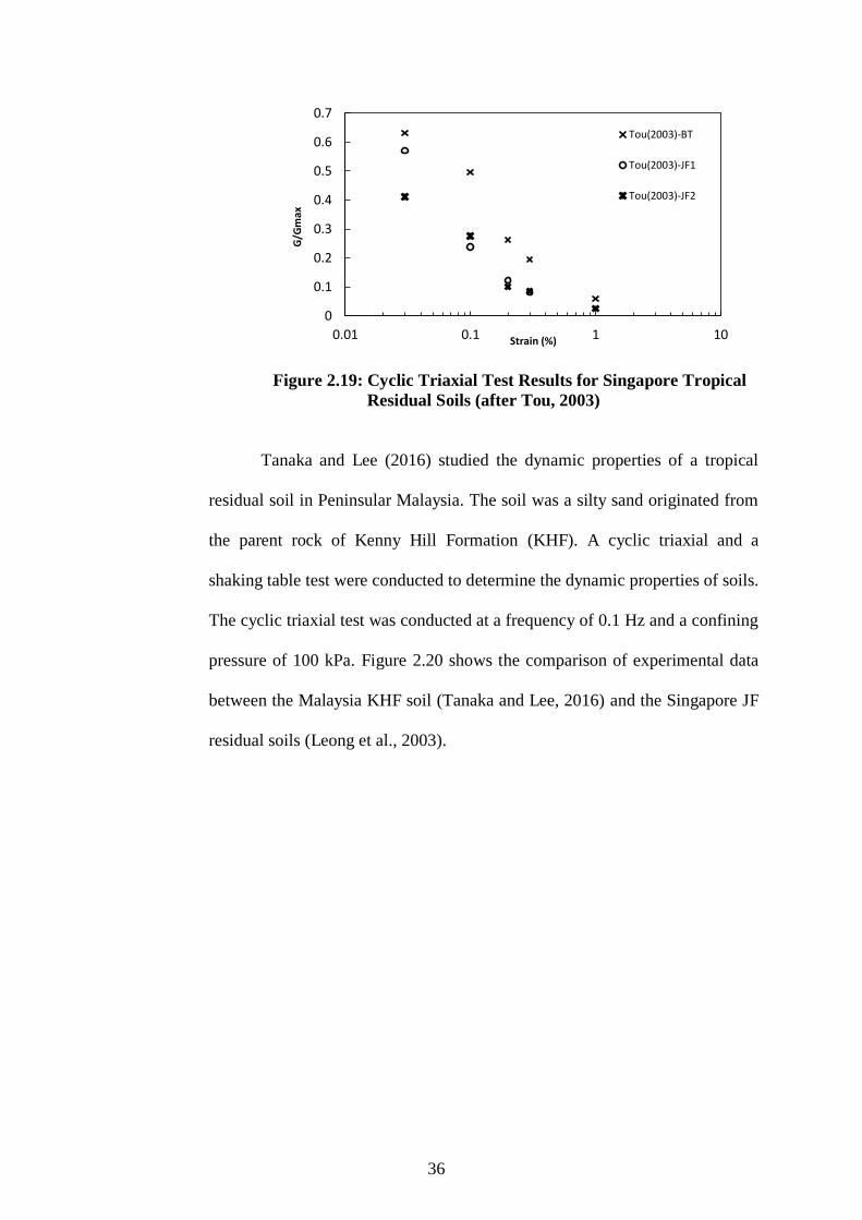
36

Figure 2.19: Cyclic Triaxial Test Results for Singapore Tropical

Residual Soils (after Tou, 2003)

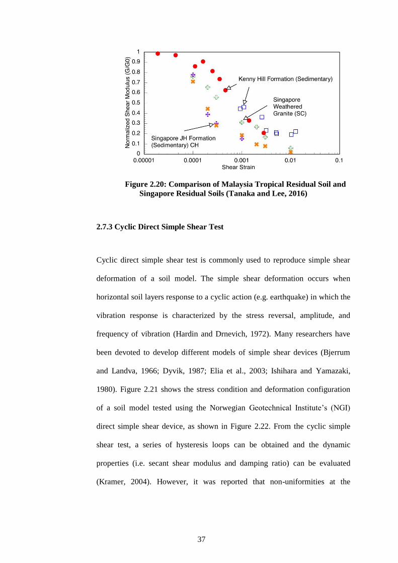
Tanaka and Lee (2016) studied the dynamic properties of a tropical

residual soil in Peninsular Malaysia. The soil was a silty sand originated from

the parent rock of Kenny Hill Formation (KHF). A cyclic triaxial and a

shaking table test were conducted to determine the dynamic properties of soils.

The cyclic triaxial test was conducted at a frequency of 0.1 Hz and a confining

pressure of 100 kPa. Figure 2.20 shows the comparison of experimental data

between the Malaysia KHF soil (Tanaka and Lee, 2016) and the Singapore JF

residual soils (Leong et al., 2003).

0

0.1

0.2

0.3

0.4

0.5

0.6

0.7

0.01 0.1 1 10

G/G

max

Strain (%)

Tou(2003)-BT

Tou(2003)-JF1

Tou(2003)-JF2

37

Figure 2.20: Comparison of Malaysia Tropical Residual Soil and

Singapore Residual Soils (Tanaka and Lee, 2016)

2.7.3 Cyclic Direct Simple Shear Test

Cyclic direct simple shear test is commonly used to reproduce simple shear

deformation of a soil model. The simple shear deformation occurs when

horizontal soil layers response to a cyclic action (e.g. earthquake) in which the

vibration response is characterized by the stress reversal, amplitude, and

frequency of vibration (Hardin and Drnevich, 1972). Many researchers have

been devoted to develop different models of simple shear devices (Bjerrum

and Landva, 1966; Dyvik, 1987; Elia et al., 2003; Ishihara and Yamazaki,

1980). Figure 2.21 shows the stress condition and deformation configuration

of a soil model tested using the Norwegian Geotechnical Institute’s (NGI)

direct simple shear device, as shown in Figure 2.22. From the cyclic simple

shear test, a series of hysteresis loops can be obtained and the dynamic

properties (i.e. secant shear modulus and damping ratio) can be evaluated

(Kramer, 2004). However, it was reported that non-uniformities at the

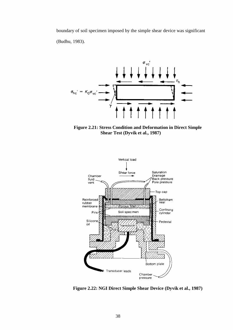
38

boundary of soil specimen imposed by the simple shear device was significant

(Budhu, 1983).

Figure 2.21: Stress Condition and Deformation in Direct Simple

Shear Test (Dyvik et al., 1987)

Figure 2.22: NGI Direct Simple Shear Device (Dyvik et al., 1987)

39

Besides, a double specimen direct simple shear device (DSDSS) and a

two-directional simple shear device were developed to investigate the dynamic

behaviours of soil (Elia et al., 2003; Ishihara and Yamazaki, 1980). Figure

2.23 shows the schematic diagram of the DSDSS device, while Figure 2.24

shows the hysteresis loop obtained from the testing.

Figure 2.23: Schematic Diagram of Double Specimens Direct

Simple Shear Device (Lanzo et al., 1997)

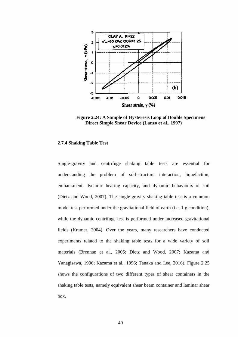
40

Figure 2.24: A Sample of Hysteresis Loop of Double Specimens

Direct Simple Shear Device (Lanzo et al., 1997)

2.7.4 Shaking Table Test

Single-gravity and centrifuge shaking table tests are essential for

understanding the problem of soil-structure interaction, liquefaction,

embankment, dynamic bearing capacity, and dynamic behaviours of soil

(Dietz and Wood, 2007). The single-gravity shaking table test is a common

model test performed under the gravitational field of earth (i.e. 1 g condition),

while the dynamic centrifuge test is performed under increased gravitational

fields (Kramer, 2004). Over the years, many researchers have conducted

experiments related to the shaking table tests for a wide variety of soil

materials (Brennan et al., 2005; Dietz and Wood, 2007; Kazama and

Yanagisawa, 1996; Kazama et al., 1996; Tanaka and Lee, 2016). Figure 2.25

shows the configurations of two different types of shear containers in the

shaking table tests, namely equivalent shear beam container and laminar shear

box.

41

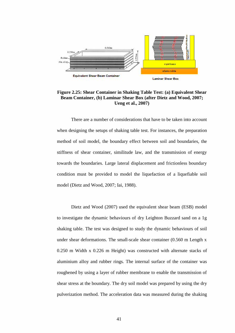
Figure 2.25: Shear Container in Shaking Table Test: (a) Equivalent Shear

Beam Container, (b) Laminar Shear Box (after Dietz and Wood, 2007;

Ueng et al., 2007)

There are a number of considerations that have to be taken into account

when designing the setups of shaking table test. For instances, the preparation

method of soil model, the boundary effect between soil and boundaries, the

stiffness of shear container, similitude law, and the transmission of energy

towards the boundaries. Large lateral displacement and frictionless boundary

condition must be provided to model the liquefaction of a liquefiable soil

model (Dietz and Wood, 2007; Iai, 1988).

Dietz and Wood (2007) used the equivalent shear beam (ESB) model

to investigate the dynamic behaviours of dry Leighton Buzzard sand on a 1g

shaking table. The test was designed to study the dynamic behaviours of soil

under shear deformations. The small-scale shear container (0.560 m Length x

0.250 m Width x 0.226 m Height) was constructed with alternate stacks of

aluminium alloy and rubber rings. The internal surface of the container was

roughened by using a layer of rubber membrane to enable the transmission of

shear stress at the boundary. The dry soil model was prepared by using the dry

pulverization method. The acceleration data was measured during the shaking

42

table test. High-pass Butterworth filtering was performed on the measured

acceleration record to obtain the displacement profiles and subsequently the

dynamic properties of soil. The dynamic properties over a wide range of shear

strain amplitudes (i.e. 0.001 % - 6 %) were determined from the experiment.

Besides, the performance of the shear box was assessed by monitoring the

end-wall deflection of the soil model.

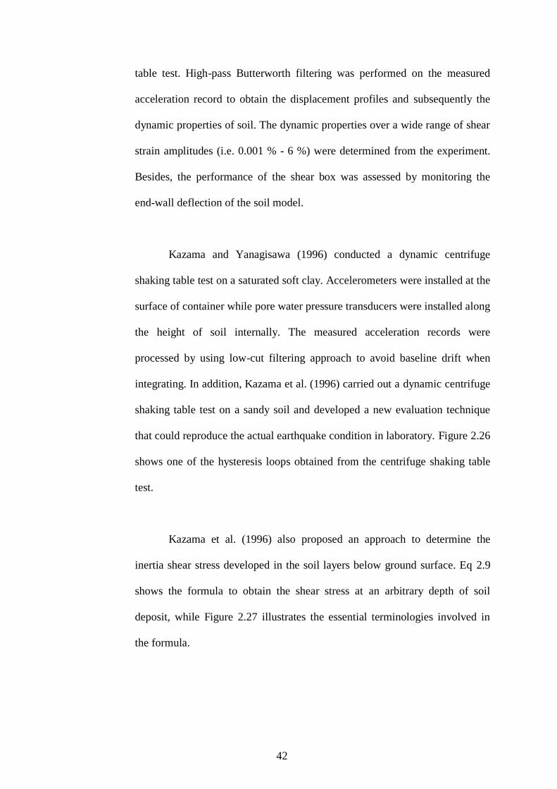
Kazama and Yanagisawa (1996) conducted a dynamic centrifuge

shaking table test on a saturated soft clay. Accelerometers were installed at the

surface of container while pore water pressure transducers were installed along

the height of soil internally. The measured acceleration records were

processed by using low-cut filtering approach to avoid baseline drift when

integrating. In addition, Kazama et al. (1996) carried out a dynamic centrifuge

shaking table test on a sandy soil and developed a new evaluation technique

that could reproduce the actual earthquake condition in laboratory. Figure 2.26

shows one of the hysteresis loops obtained from the centrifuge shaking table

test.

Kazama et al. (1996) also proposed an approach to determine the

inertia shear stress developed in the soil layers below ground surface. Eq 2.9

shows the formula to obtain the shear stress at an arbitrary depth of soil

deposit, while Figure 2.27 illustrates the essential terminologies involved in

the formula.

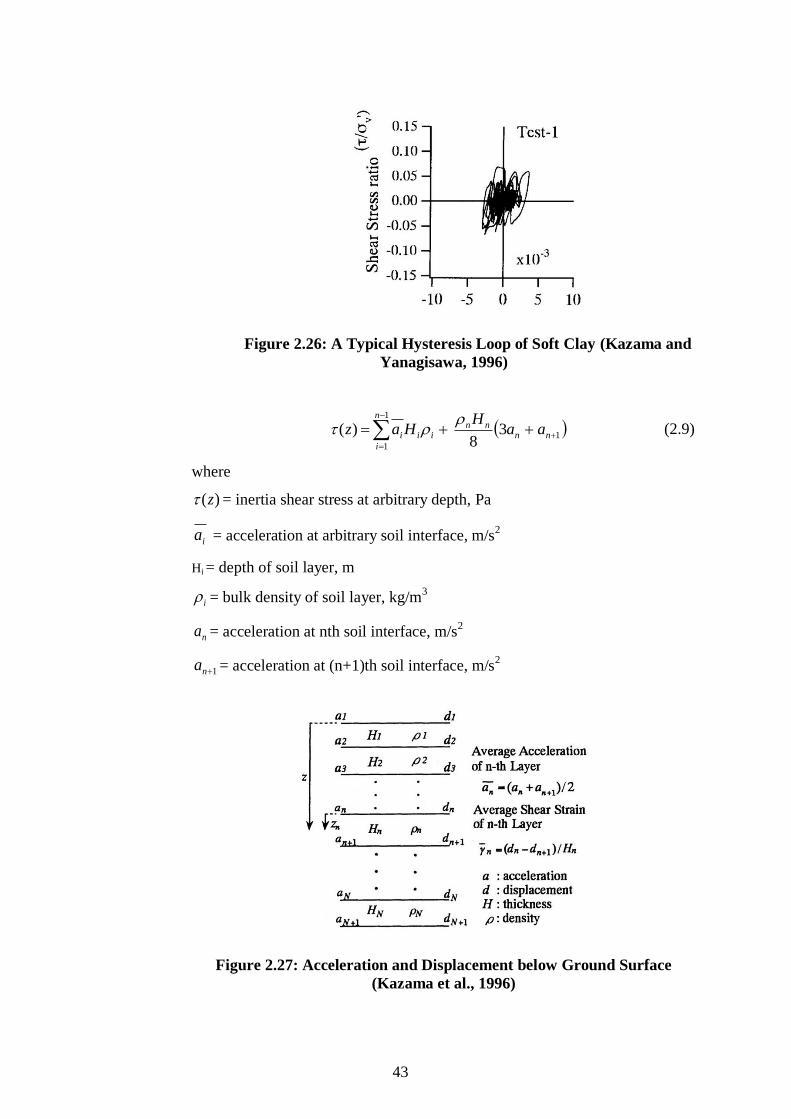
43

Figure 2.26: A Typical Hysteresis Loop of Soft Clay (Kazama and

Yanagisawa, 1996)

1

1

1

38

)(

nnnn

n

i

iii aaH

Haz

(2.9)

where

)(z = inertia shear stress at arbitrary depth, Pa

ia = acceleration at arbitrary soil interface, m/s2

Hi = depth of soil layer, m

i = bulk density of soil layer, kg/m3

na = acceleration at nth soil interface, m/s2

1na = acceleration at (n+1)th soil interface, m/s2

Figure 2.27: Acceleration and Displacement below Ground Surface

(Kazama et al., 1996)

44

Tanaka and Lee (2016) conducted a 1g shaking table test on a sandy

soil in Malaysia. The soil model, which was originated from the Kenny Hill

Formation, was compacted to the designated volume in which the soil

condition in a compacted embankment could be reproduced. Accelerometers

were installed to monitor the changes of acceleration with time and baseline

correction was performed to avoid the baseline drift. The dynamic properties

were obtained from a series of hysteresis loops. However, the integrated

displacement data from accelerometers were subjected to certain degrees of

uncertainties. Therefore, a direct displacement measurement technique has to

be performed to obtain accurate and reliable results. Slifka (2004) used laser

displacement sensor as a reference when processing the measured acceleration

data of a moving object. They also reported an acceptable difference of

displacement between the measurements obtained from the laser displacement

sensor and the displacement derived from the acceleration record. In light of

the non-destructive nature and the accurate measurement on dynamic

movement of an object, laser displacement sensor can serve as a favourable

option for measuring a small deformation of soil specimens.

Dynamic properties covering a specific range of shear strain

amplitudes can be obtained from the 1g shaking table tests, but it was limited

by the low confining pressure exerted on the soil model. Table 1 summarizes

the confining pressure and shear strain ranges that have been successfully

achieved by using the 1g shaking table test from the previous studies (Araei

and Towhata 2014, Dietz and Muir Wood 2007, Tsai et al. 2016, Tanaka and

45

Lee 2016). The confining pressures are generally limited to below 30 kPa and

the ranges of shear strain amplitudes lay in between 0.01% and 1%.

Table 2.2: Confining Pressures and Strain Ranges Reported in Previous

1g Shaking Table Tests

Literature Confining

Pressure

Strain Range (%)

Araei and Towhata (2014) <16kPa 0.014 - 1.200

Dietz and Muir Wood (2007) 8.4kPa 0.010 –0.600

Tsai and et al. (2016) <30kPa 0.010 –0.100

Tanaka and Lee (2016) <10kPa 0.092 – 1.257

From the preceding literature review on the shaking table test for soil,

it can be inferred that the shaking table test is not only capable of facilitating

the study of liquefaction, but also can be used to reproduce the simple shear

deformation of a soil model. The deformation behaviour of a soil model,

which is subjected to a dynamic event, can be experimentally determined

using accurate measuring transducers/ devices (i.e. accelerometer, LVDT,

laser displacement sensor).

2.8 Signal Processing

2.8.1 Earthquake Records

Acceleration records can be measured by using accelerograph, seismograph or

accelerometer during an earthquake event (Kramer, 2004). Figure 2.28 shows

the acceleration, velocity, and displacement records of a selected

accelerograph station during the 1999 Chi-Chi, Taiwan earthquake. The

acceleration records shown were measured in three orthogonal directions. The

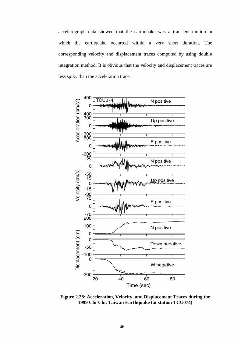
46

accelerograph data showed that the earthquake was a transient motion in

which the earthquake occurred within a very short duration. The

corresponding velocity and displacement traces computed by using double

integration method. It is obvious that the velocity and displacement traces are

less spiky than the acceleration trace.

Figure 2.28: Acceleration, Velocity, and Displacement Traces during the

1999 Chi-Chi, Taiwan Earthquake (at station TCU074)

47

Important ground motion parameters can be derived from the

acceleration records through a series of data processing approaches. Ground

motion parameters and their characteristics are of importance to seismologists,

geologists, and earthquake engineers. Among many parameters, residual

displacement is essential for investigating the fault rupture after the occurrence

of a strong ground motion. The permanent or residual displacement could be

caused by plastic deformation of near-surface material or elastic deformation

of ground as the result of co-seismic slip on the fault (Boore and Bommer,

2005).

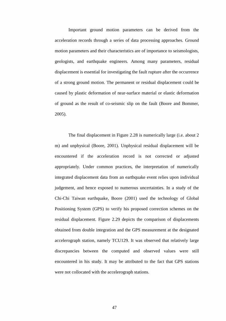
The final displacement in Figure 2.28 is numerically large (i.e. about 2

m) and unphysical (Boore, 2001). Unphysical residual displacement will be

encountered if the acceleration record is not corrected or adjusted

appropriately. Under common practices, the interpretation of numerically

integrated displacement data from an earthquake event relies upon individual

judgement, and hence exposed to numerous uncertainties. In a study of the

Chi-Chi Taiwan earthquake, Boore (2001) used the technology of Global

Positioning System (GPS) to verify his proposed correction schemes on the

residual displacement. Figure 2.29 depicts the comparison of displacements

obtained from double integration and the GPS measurement at the designated

accelerograph station, namely TCU129. It was observed that relatively large

discrepancies between the computed and observed values were still

encountered in his study. It may be attributed to the fact that GPS stations

were not collocated with the accelerograph stations.

48

Figure 2.29: Comparison of Displacements obtained from Double

Integration and GPS Measurement (after Boore, 2001)

2.8.2 Baseline Correction

The unphysical residual displacement as shown in Figure 2.28 is attributed to

the baseline drift and the initial condition in numerical integration. At the end

of each shaking motion, the velocity should become zero while certain amount

of residual displacement could be expected (Boore and Bommer, 2005). Over

the years, numerous adjustment schemes for processing seismic records have

been proposed by many researchers worldwide (Iwan et al., 1985; Ohsaki,

1995; Chiu, 1997; Boore, 2001). Although there are various correction

schemes proposed to recover the actual shaking record, it is almost impossible

to recover an earthquake record perfectly.

49

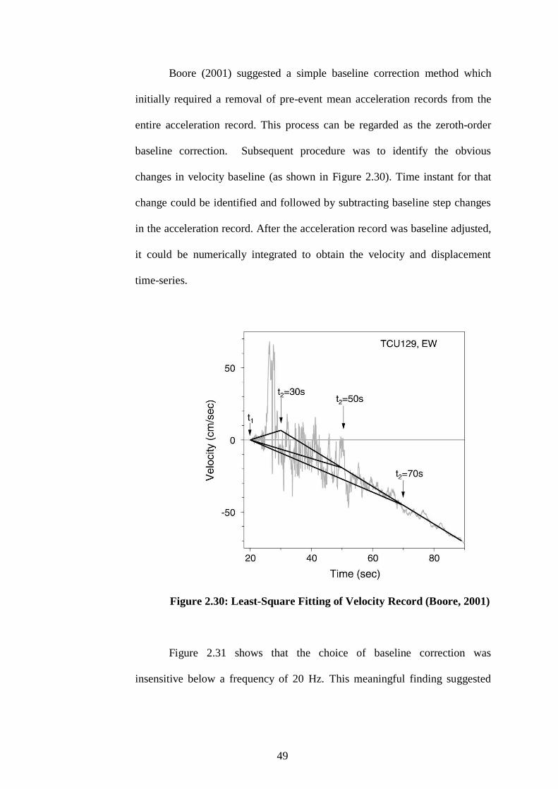
Boore (2001) suggested a simple baseline correction method which

initially required a removal of pre-event mean acceleration records from the

entire acceleration record. This process can be regarded as the zeroth-order

baseline correction. Subsequent procedure was to identify the obvious

changes in velocity baseline (as shown in Figure 2.30). Time instant for that

change could be identified and followed by subtracting baseline step changes

in the acceleration record. After the acceleration record was baseline adjusted,

it could be numerically integrated to obtain the velocity and displacement

time-series.

Figure 2.30: Least-Square Fitting of Velocity Record (Boore, 2001)

Figure 2.31 shows that the choice of baseline correction was

insensitive below a frequency of 20 Hz. This meaningful finding suggested

50

that most of the structures under seismic activities would not be affected by

the choice of baseline correction methods.

Figure 2.31: Displacement Response Spectra (Boore, 2005)

In Japan, Ohsaki (1995) suggested a well-known baseline correction

procedure which was fundamentally based on the assumptions that velocity at

the end of shaking would return to zero whilst certain amount of residual

displacement could be expected.

In addition, Chiu (1997) suggested a “stable” three-step algorithm

baseline correction scheme for processing digital strong motion data. This

method involved least-square fitting in acceleration record, high-pass filtering

in acceleration record, and subtracting the initial velocity value. Figure 2.32

shows the acceleration and displacement records using the approach proposed

by Chiu (1997).

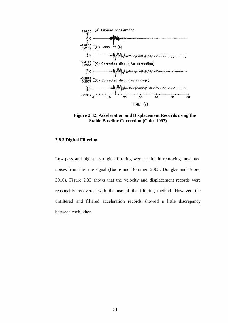
51

Figure 2.32: Acceleration and Displacement Records using the

Stable Baseline Correction (Chiu, 1997)

2.8.3 Digital Filtering

Low-pass and high-pass digital filtering were useful in removing unwanted

noises from the true signal (Boore and Bommer, 2005; Douglas and Boore,

2010). Figure 2.33 shows that the velocity and displacement records were

reasonably recovered with the use of the filtering method. However, the

unfiltered and filtered acceleration records showed a little discrepancy

between each other.

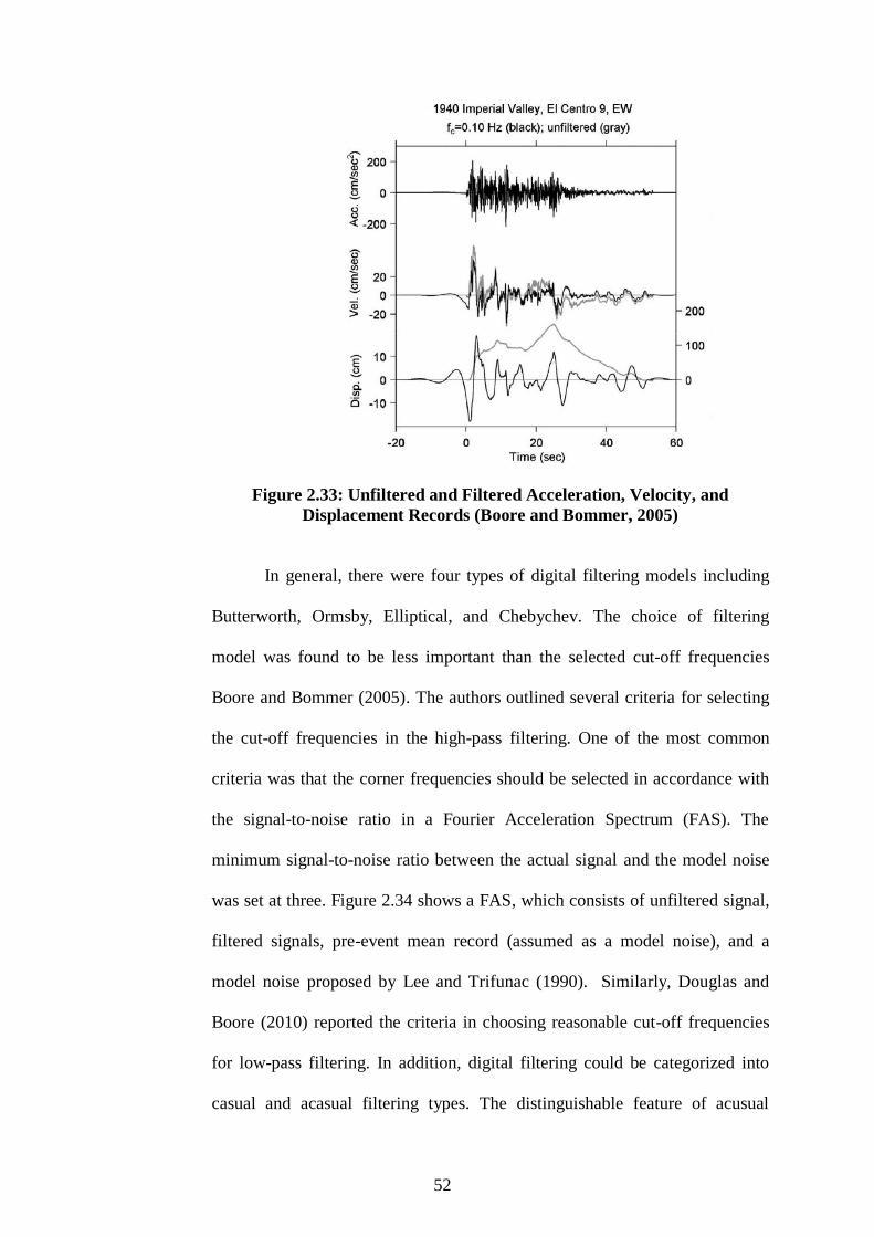
52

Figure 2.33: Unfiltered and Filtered Acceleration, Velocity, and

Displacement Records (Boore and Bommer, 2005)

In general, there were four types of digital filtering models including

Butterworth, Ormsby, Elliptical, and Chebychev. The choice of filtering

model was found to be less important than the selected cut-off frequencies

Boore and Bommer (2005). The authors outlined several criteria for selecting

the cut-off frequencies in the high-pass filtering. One of the most common

criteria was that the corner frequencies should be selected in accordance with

the signal-to-noise ratio in a Fourier Acceleration Spectrum (FAS). The

minimum signal-to-noise ratio between the actual signal and the model noise

was set at three. Figure 2.34 shows a FAS, which consists of unfiltered signal,

filtered signals, pre-event mean record (assumed as a model noise), and a

model noise proposed by Lee and Trifunac (1990). Similarly, Douglas and

Boore (2010) reported the criteria in choosing reasonable cut-off frequencies

for low-pass filtering. In addition, digital filtering could be categorized into

casual and acasual filtering types. The distinguishable feature of acusual

53

filtering is that it would not produce any phase shift in the records. This can be

accomplished by adding a line of data with zero amplitude, which is known as

pad, before the starting of a record and after the end of the record. The length

of pads depends on the filter frequency and filter order (Boore and Bommer,

2005). Boore and Bommer (2005) also opined that the pre-event and post-

event records were not often sufficient for the acasual filtering.

Figure 2.34: Fourier Acceleration Spectrum of Unfiltered and Filtered

Acceleration Records (Boore and Bommer, 2005)

Mollova (2006) presented the application of digital filtering using a

commercial software, namely SeismoSignal to process an actual earthquake

record in Turkey. SeismoSignal is one of the popular commercial software that

can be used to process earthquake strong-motion data with the function of

graphical user interface. Baseline correction and digital filtering methods are

incorporated in the software package. The effects of using various types of

54

digital filtering models (i.e. Chebyshev, Butterworth, Bessel, and Elliptic)

were examined in detail. Mollova (2006) examined the influences of filtering

types (i.e. Butterworth, Chebyshev, and Bessel) and the order of filtering on

the acceleration, velocity, and displacement time series. In addition, the

Fourier Amplitude Spectra and the response spectra (with damping

characteristics of 5 %) the dynamic event were evaluated.

2.9 Concluding Remarks

In summary, Malaysia is a tropical country with abundant of residual soils

covering the superficial soil deposits. Recent occurrences of earthquakes and

tremors have attracted increasing attention from the public in Malaysia. From

the review of the current available literature, it can be concluded that studies

on soil dynamics are still very limited in Malaysia. More experimental testing

should be carried out to enrich the current database of soil dynamic properties,

particularly for tropical residual soil.

From the literature, shear modulus degradation curves as well as the

relationships between damping ratio and shear strain amplitude were widely

used to describe the dynamic behaviours of soil. The effects of density,

effective confining pressure, plasticity index, shear strain amplitude, and etc.

on soil dynamic properties were examined. The effects of density and effective

confining pressure are profound in sandy soil, while the effect of plasticity

index and rate of loading are significant in clayey soil. From the foregoing

literature study, it is beneficial to compare the experimental data of selected

tropical residual soils in Malaysia with the above-mentioned degradation

55

curves of sand and clay. This is because tropical residual soils are peculiarly

characterized with sand-to-clay mixture. The effects of the above-mentioned

parameters on tropical residual soil, such as confining pressure, plasticity

index, shear strain amplitude, and soil type, can be investigated in further

detail.

A number of soil dynamic testing was reviewed, such as cyclic triaxial

test, cyclic torsional shear test, cyclic simple shear test, shaking table test, and

etc. Shaking table test was found to be useful in providing reasonable

representation of seismic soil response. However, the confining pressures are

generally limited to below 30 kPa and the ranges of shear strain amplitudes lay

in between 0.01 % and 1 % on a 1g shaking table.

Appropriate signal processing is required to process the acceleration

records from an earthquake or a dynamic test. Baseline correction and digital

filtering methods are essential to remove the low and high-frequency noises

from an actual signal. However, the integrated displacement data from an

accelerometer record is often subjected to uncertainties. Therefore, a direct

displacement measurement should be used as a reference when processing the

measured acceleration records.

CHAPTER 3

METHODOLOGY

3.1 Introduction

From a variety of available soil dynamic tests, the shaking table test is selected

in the present study because it can facilitate the investigation of dynamic

behaviour of tropical residual soils and the apparatus is readily available in the

laboratory of the author’s institution. This chapter describes the methodology

of soil sampling, physical tests, development of testing setups,

instrumentation, and testing parameters.

3.2 Soil Sampling and Physical Tests

3.2.1 Soil Sampling

Three types of soil were sampled from the superficial layer (i.e. at about 2 m

below ground surface) at the selected sites in Peninsular Malaysia. The soil

samples consisted of a sand mining trail and two typical types of tropical

residual soil. The sand mining trail was sampled from a site at Bandar Sunway

(Soil C), while the two samples of tropical residual soils were collected from a

site at Kajang (Soil A) and a site at Simpang Renggam (Soil B), respectively.

The sand mining trail was not a typical tropical residual soil but it was studied

for comparison purposes because the dynamic behaviour of sandy soil has

been well established in the previous literature.

57

Figure 3.1 shows the locations of the sampling sites. In general, the

residual soils in Peninsular Malaysia can be grouped into two categories,

namely granitic residual soil and sedimentary residual soil. Based on the

locations of the sampling sites as shown in the Figure 3.1, the two tropical

residual soils (i.e. Soil A and Soil B) are originated from the sedimentary rock.

In specific, the soil deposit of Kajang formation (Soil A) belongs to a

metasedimentary rock formation which consists of schist and phyllite (Gue

and Wong, 2009). The soil in Simpang Renggam area (Soil B) is originated

from a clastic sedimentary rock formation which consists of shale material

(Tan and Azwari, 2001). In tropical countries, schist and shale would produce

mostly silty materials or soils with illitic clay minerals. Apart from the

physical weathering process, chemical weathering is prevalence in hot and

humid regions in which the rock is decomposed into silty or clayey residual

soils (Huat et al., 2012). In terms of the geological age of rock, the Kajang

schist is within the Silurian and Ordovician periods, whereas the rock of

Simpang Renggam is in the middle to late Permian period. The Permian

period is earlier than the Silurian and Ordovician period (Foo, 1983).

58

Figure 3.1: Locations of Soil Sampling Sites

3.2.2 Soil Physical Tests

Soil disaggregation and standard physical tests were performed upon

collection of the soil samples. Firstly, unwanted debris and substances were

removed from the collected soils. The soils were oven-dried at 105 ºC for 24

hours. The soil physical tests were subsequently conducted in compliance with

59

the procedures as stated in the British Standard, BS 1377: Part 2 (BSI, 1990).

The physical tests included wet sieving, hydrometer analysis, Atterberg limit

tests, and proctor compaction test.

3.3 Apparatus and Instrumentation

3.3.1 Shaking Table System

A 1g shaking table machine was used to investigate the dynamic responses of

soils under a series of designated shaking motions. Figure 3.2 shows the

schematic diagram and photographs of the shaking table system. A direct-

drive motor was used to produce a one-dimensional shaking motion on a

levelled shaking table platform (2 m by 2 m) by generating a mechanical

torque repeatedly. The shaking table platform was lifted upward by supplying

an air pressure of 2 bars beneath. The air pressure, which was controlled by an

air regulator, was supplied through the evenly distributed outlets beneath the

platform for enabling the shaking table to move freely in the horizontal

direction. An aluminium panel and a layer of foam were also attached beneath

the shaking table platform for facilitating a uniform movement.

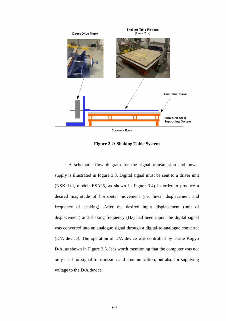
60

Figure 3.2: Shaking Table System

A schematic flow diagram for the signal transmission and power

supply is illustrated in Figure 3.3. Digital signal must be sent to a driver unit

(NSK Ltd, model: ESA25, as shown in Figure 3.4) in order to produce a

desired magnitude of horizontal movement (i.e. linear displacement and

frequency of shaking). After the desired input displacement (unit of

displacement) and shaking frequency (Hz) had been input, the digital signal

was converted into an analogue signal through a digital-to-analogue converter

(D/A device). The operation of D/A device was controlled by Turtle Kogyo

D/A, as shown in Figure 3.5. It is worth mentioning that the computer was not

only used for signal transmission and communication, but also for supplying

voltage to the D/A device.

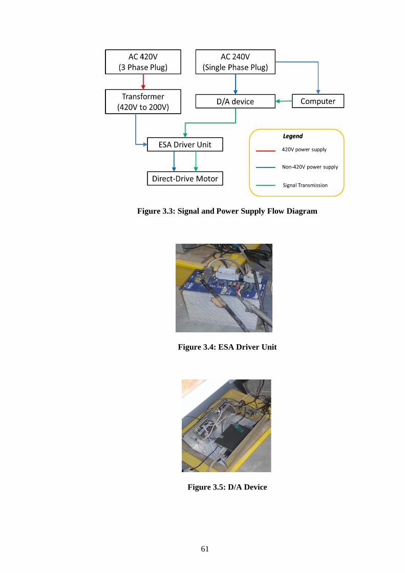
61

Figure 3.3: Signal and Power Supply Flow Diagram

Figure 3.4: ESA Driver Unit

Figure 3.5: D/A Device

62

Figure 3.6 shows the graphical user interface (GUI) of the computer

program, MOTCTLPROG (3DA-GATECTRL), which was used to input the

shaking motions. The computer program was written using Visual Basic for

Applications (VBA) programming code.

Figure 3.6: Graphical User Interface of MOTCTLPROG

The common input frequencies ranged from 0.1 Hz to 20 Hz, while the

input linear displacements ranged from 0.1 to 8 unit of displacement.

However, it was realized that the actual horizontal displacement was not

identical with the numeric value of input displacement. Therefore, it was

required to calibrate and measure the actual horizontal displacement of the

shaking table using device laser displacement sensor.

63

3.3.2 Accelerometer

Accelerometers were used to monitor the changes of acceleration with time

during the shaking table test. Three units of TML accelerometers (model:

ARH-20A) and five units of KYOWA accelerometers (model: ASW-2A) were

used for the experiment. The TML accelerometer has an acceleration

measuring range from 10 m/s2 to 500 m/s

2, while the KYOWA accelerometer

has an acceleration measuring range from 9.807 m/s2 to 196.1 m/s

2. Both of

the accelerometers can withstand a water pressure up to 500 kPa (5 bars). It is

worth noting that a glass plate of 2 mm thickness was screwed onto the surface

of the accelerometers in order to provide a uniform contact surface with soil

when subjected to vibration (refer to Figure 3.7a). For measurements on a

metal surface, the accelerometers were attached directly on the surface by

using adhesive-tape mounting method (refer to Figure 3.7b). This mounting

method has an advantage of providing electrical insulation between

accelerometer and the metal contact surface (Piersol and Paez, 2010).

Figure 3.7a: Accelerometer attached on Soil Surface

64

Figure 3.7b: Accelerometer attached on Metal Surface

3.3.3 Laser Displacement Sensor

Laser displacement sensors were utilized to monitor the changes of linear

displacement with time accurately. Within a certain measuring range, this type

of non-destructive device is able to detect the linear displacement directly

without disturbing the test specimen. The model of the laser displacement

sensors used in the present study was OPTEX FA CD5-85, as shown in Figure

3.8. It has a measuring range of 85 ± 20 mm with a measuring resolution of 1

µm and a minimum sampling interval as low as 100 µs.

Figure 3.8: Laser Displacement Sensor Head (CD5-85)

An amplifier/ controller was required to monitor and store the linear

displacement readings digitally (as shown in Figure 3.9). Voltage ranged from

65

12 V to 24 V can be transmitted to the amplifier through a power supply

driver. A USB cable was used to connect the amplifier to a computer in order

to monitor and store the measured data through a GUI software, namely

Sensor Navigation (Figure 3.10).

Figure 3.9: Amplifier

Figure 3.10: Interface of Sensor Navigation

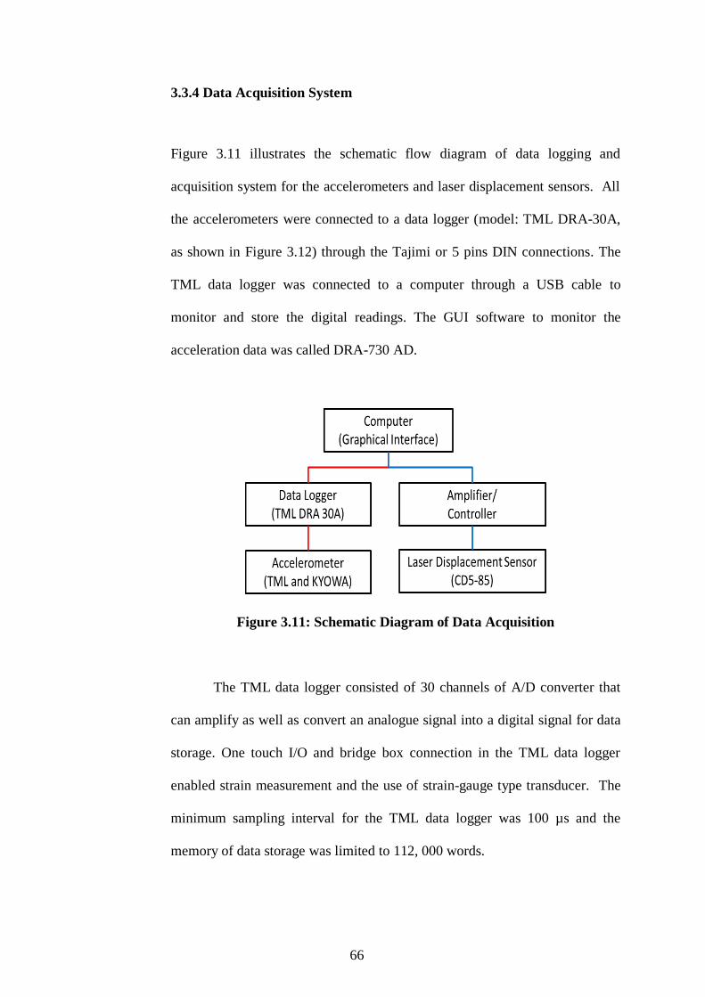
66

3.3.4 Data Acquisition System

Figure 3.11 illustrates the schematic flow diagram of data logging and

acquisition system for the accelerometers and laser displacement sensors. All

the accelerometers were connected to a data logger (model: TML DRA-30A,

as shown in Figure 3.12) through the Tajimi or 5 pins DIN connections. The

TML data logger was connected to a computer through a USB cable to

monitor and store the digital readings. The GUI software to monitor the

acceleration data was called DRA-730 AD.

Figure 3.11: Schematic Diagram of Data Acquisition

The TML data logger consisted of 30 channels of A/D converter that

can amplify as well as convert an analogue signal into a digital signal for data

storage. One touch I/O and bridge box connection in the TML data logger

enabled strain measurement and the use of strain-gauge type transducer. The

minimum sampling interval for the TML data logger was 100 µs and the

memory of data storage was limited to 112, 000 words.

67

Figure 3.12: TML Data Logger (TML DRA-30A)

3.4 Calibration of Devices

3.4.1 Calibration of Shaking Table System

A series of trial tests were first carried out by using a laser displacement

sensor to determine the feasible shaking magnitudes and the consistency of the

input and actual shaking motions of the shaking table. During the trial tests,

two important considerations were taken into account: (1) the movement of

the shaking table must not be significantly affected by noises, and (2) the

movement must be within the measuring range of the laser displacement

sensor. The results of the trial tests are presented in Figure 3.13. The feasible

shaking magnitudes were represented by the shaded zone below the envelope.

Figure 3.13 shows that a shaking magnitude with a high input frequency

should be coupled with a low input displacement, and vice versa. For

instances, a low input shaking frequency of 1 Hz permitted a maximum input

displacement of 2 unit of displacement. However, at an input frequency of 20

Hz, the maximum input displacement was only limited to 0.1 unit of

displacement.

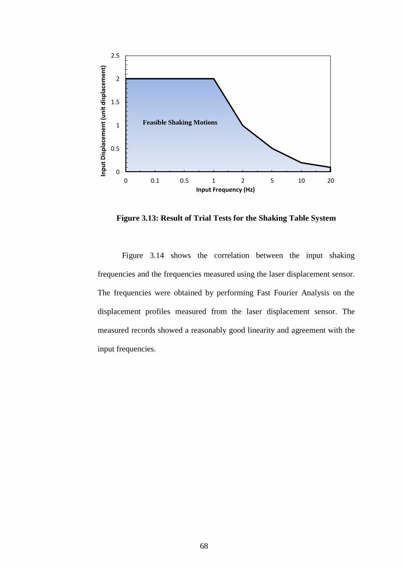
68

Figure 3.13: Result of Trial Tests for the Shaking Table System

Figure 3.14 shows the correlation between the input shaking

frequencies and the frequencies measured using the laser displacement sensor.

The frequencies were obtained by performing Fast Fourier Analysis on the

displacement profiles measured from the laser displacement sensor. The

measured records showed a reasonably good linearity and agreement with the

input frequencies.

0

0.5

1

1.5

2

2.5

0 0.1 0.5 1 2 5 10 20

Inp

ut

Dis

pla

cem

ent

(un

it d

isp

lace

men

t)

Input Frequency (Hz)

Feasible Shaking Motions

69

Figure 3.14: Relationships between Measured and Input Frequencies

Figure 3.15 depicts the relationship between the input displacements

and the displacements measured by using the laser displacement sensor. In

general, the actual displacements were found to be higher than those of input

values. At frequencies of 0.5 – 5 Hz, a good linearity and consistency was

observed in which the measured displacement was about 3.7 times higher than

the input displacement. However, at the high frequency of 5 Hz, the linearity

was only valid up to 0.5 unit of displacement. At an extremely low frequency,

i.e. 0.1 Hz, even though the shaking table was still capable of showing a linear

relationship between the input and measured displacements, the correlation

constant was found to be at 2.4, which was considerably lower than the

constant of 3.7 for other higher input frequencies.

y = 1.0549x R² = 0.9889

0

2

4

6

8

10

12

0 2 4 6 8 10 12

Me

asu

red

Fre

qu

en

cy (

Hz)

Input Frequency (Hz)

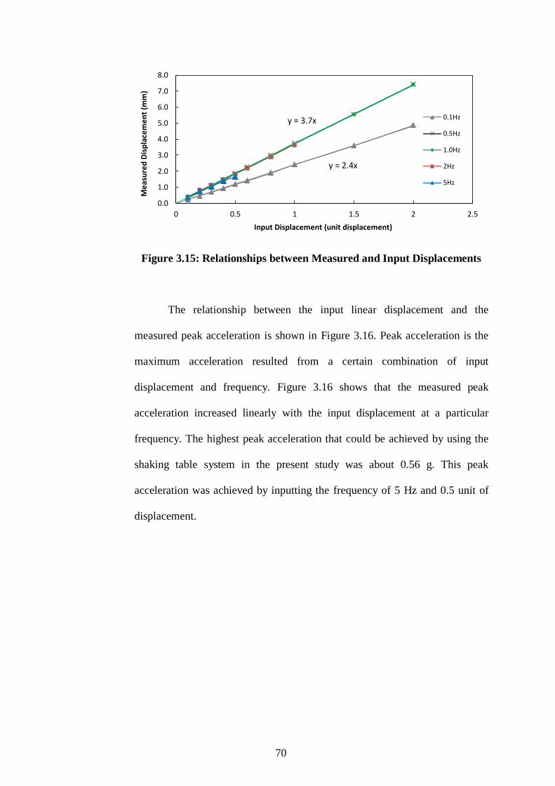
70

Figure 3.15: Relationships between Measured and Input Displacements

The relationship between the input linear displacement and the

measured peak acceleration is shown in Figure 3.16. Peak acceleration is the

maximum acceleration resulted from a certain combination of input

displacement and frequency. Figure 3.16 shows that the measured peak

acceleration increased linearly with the input displacement at a particular

frequency. The highest peak acceleration that could be achieved by using the

shaking table system in the present study was about 0.56 g. This peak

acceleration was achieved by inputting the frequency of 5 Hz and 0.5 unit of

displacement.

y = 2.4x

y = 3.7x

0.0

1.0

2.0

3.0

4.0

5.0

6.0

7.0

8.0

0 0.5 1 1.5 2 2.5

Me

asu

red

Dis

pla

cem

en

t (m

m)

Input Displacement (unit displacement)

0.1Hz

0.5Hz

1.0Hz

2Hz

5Hz

71

Figure 3.16: Relationships between Peak Acceleration and Input

Displacement

3.4.2 Calibration of Accelerometers

There were three calibrated TML accelerometers and five uncalibrated

KYOWA accelerometers used in the present study. A well-calibrated TML

accelerometer (i.e. with a code number of 52144) was used as the benchmark

for calibration of other accelerometers. The calibration of accelerometers was

carried out by correlating the unknown accelerometers with respect to a

calibrated accelerometer. All accelerometers were mounted on the shaking

table and subjected to a series of cyclic movements. Acceleration data (m/s2)

for each accelerometer was computed by multiplying a coefficient with the

recorded output voltage data (mV). For the KYOWA accelerometers, the

initial coefficients were assumed to be 0.018. The calibrated coefficients for

all KYOWA accelerometers were obtained by multiplying the initial

coefficient with improvement ratios, which were the gradients of best-fit linear

lines obtained from relationships between the acceleration data of calibrated

0

1

2

3

4

5

6

0 1 2 3 4 5 6 7 8

Pe

ak A

cce

lera

tio

n (

m/s

2 )

Input Displacement (unit displacement)

0.5Hz 1.0Hz 2.0Hz 5.0Hz

72

TML and KYOWA accelerometers. Table 3.1 summarizes the coefficients of

calibration for each accelerometer.

Table 3.1: Calibration of Accelerometers

Brand Accelerometer

Code Number

Initial

Coefficient

Improvement

Ratio

Calibrated

Coefficient

TML 52144(benchmark) 0.0212 - 0.0212

TML 52145 0.0227 - 0.0227

TML DFC-04062 0.0233 - 0.0233

KYOWA EQ-1590012 0.0180 1.0598 0.0190764

KYOWA EP-5500001 0.0180 1.0900 0.01962

KYOWA EQ-1590010 0.0180 1.1074 0.0199332

KYOWA EQ-1590007 0.0180 1.0900 0.01962

KYOWA EQ-1590008 0.0180 1.0710 0.019278

3.5 Setups of Testing Models

There were three main setups used for the shaking table test including a large

laminar shear box test (LLSBT), a small chamber test with positive air

pressure (SCT) and a small sample test with suction (SSTS). These tests were

carried out on the 1g shaking table and subjected to a series of cyclic

movements. In the following sub-sections, the methodology of each testing

setup will be explained explicitly.

3.5.1 Large Laminar Shear Box Test (LLSBT)

Figure 3.17 and Figure 3.18 show the schematic diagram and the photograph

of the LLSBT model used in the present study. The LLSBT setup consisted of

an aluminium laminar shear box of 1.5 m (length) x 0.7 m (width) x 0.21 m

73

(height), and a surcharge loading applied on top of the soil model to create an

overburden pressure. The soil model was instrumented with accelerometers to

monitor the acceleration during testing. The advantage of the LLSBT was that

the large sample could minimize the boundary effect and give a better

replication of the in-situ soil compared to small laboratory samples (Koo et al.,

2016).

Figure 3.17: Schematic Diagram of LLSBT

Figure 3.18: Experimental Setup for LLSBT

74

There were three layers of aluminium shear stacks used to confine the

soil model, with the height of each stack being 0.07 m. The base of the

aluminium shear stacks was rigidly clamped on the shaking table platform,

and the shear stacks were allowed to move freely relative to each other. This

was made possible by providing sliding joints between the aluminium laminar

shear stacks (as shown in Figure 3.19).

Figure 3.19: Sliding Joints on Aluminium Laminar Shear Stacks

A sheet of 0.3 mm thick rubber membrane was placed inside the

aluminium shear box (Figure 3.20). The functions of the rubber membrane

were to confine the soil model laterally and prevent dissipation of water from

the soil. Since the dimension of the rubber membrane was not available in the

commercial market, it was therefore fabricated in the laboratory using High

Ammonia Latex Concentrate.

75

Figure 3.20: Aluminium Shear Box and Rubber Membrane

For sample preparation, the soil was compacted to 95 % of the

maximum dry density. A wood tamper, which was coated with latex, was

fabricated to compact the soil sample into six successive layers (Figure 3.21).

The interface between soil layers was scratched to minimize heterogeneity in

the compacted layers of soil. Figure 3.22 shows the compacted soil model for

the LLSBT.

Figure 3.21: Compaction of Soil Layer

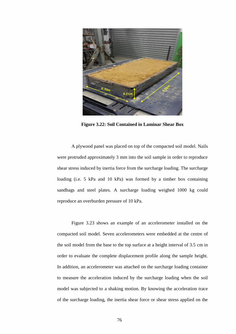
76

0.21m1.5

0m0.70m

Figure 3.22: Soil Contained in Laminar Shear Box

A plywood panel was placed on top of the compacted soil model. Nails

were protruded approximately 3 mm into the soil sample in order to reproduce

shear stress induced by inertia force from the surcharge loading. The surcharge

loading (i.e. 5 kPa and 10 kPa) was formed by a timber box containing

sandbags and steel plates. A surcharge loading weighed 1000 kg could

reproduce an overburden pressure of 10 kPa.

Figure 3.23 shows an example of an accelerometer installed on the

compacted soil model. Seven accelerometers were embedded at the centre of

the soil model from the base to the top surface at a height interval of 3.5 cm in

order to evaluate the complete displacement profile along the sample height.

In addition, an accelerometer was attached on the surcharge loading container

to measure the acceleration induced by the surcharge loading when the soil

model was subjected to a shaking motion. By knowing the acceleration trace

of the surcharge loading, the inertia shear force or shear stress applied on the

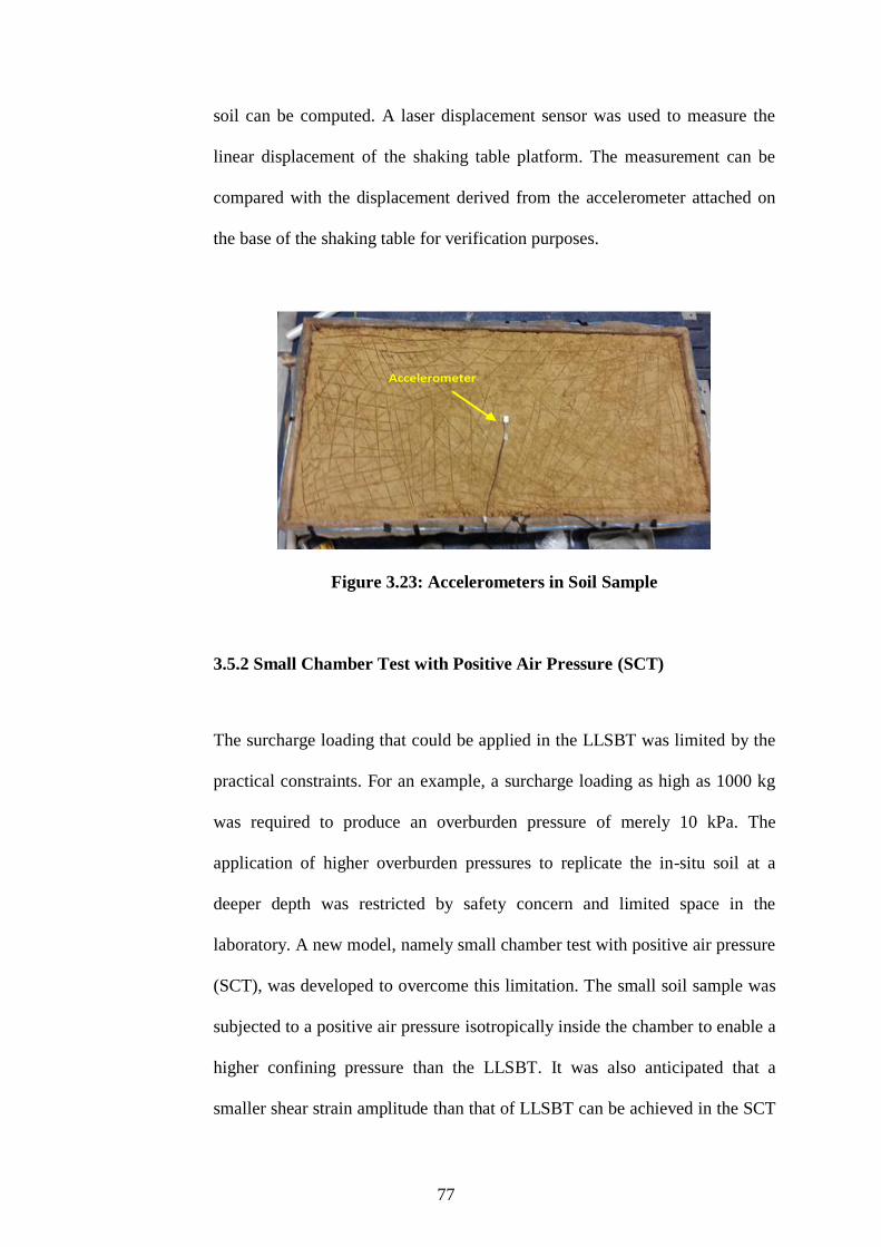
77

soil can be computed. A laser displacement sensor was used to measure the

linear displacement of the shaking table platform. The measurement can be

compared with the displacement derived from the accelerometer attached on

the base of the shaking table for verification purposes.

Accelerometer

Figure 3.23: Accelerometers in Soil Sample

3.5.2 Small Chamber Test with Positive Air Pressure (SCT)

The surcharge loading that could be applied in the LLSBT was limited by the

practical constraints. For an example, a surcharge loading as high as 1000 kg

was required to produce an overburden pressure of merely 10 kPa. The

application of higher overburden pressures to replicate the in-situ soil at a

deeper depth was restricted by safety concern and limited space in the

laboratory. A new model, namely small chamber test with positive air pressure

(SCT), was developed to overcome this limitation. The small soil sample was

subjected to a positive air pressure isotropically inside the chamber to enable a

higher confining pressure than the LLSBT. It was also anticipated that a

smaller shear strain amplitude than that of LLSBT can be achieved in the SCT

78

in order to provide insights into the deformation behaviour of soil over

different strain ranges. Figure 3.24 shows the schematic diagram and the

photograph of the SCT. The small soil sample was radially confined by

confining air pressures of 50 kPa and 100 kPa.

Figure 3.24: Setup of SCT

For sample preparation, the soil was compacted into a cylindrical

mould of 150 mm in diameter and 100 mm in height at an identical density as

that of LLSBT (as shown in Figure 3.25). The soil compaction was done in

four successive layers with the interfaces of soil layers were scratched. A

piece of filter paper was placed at the bottom of soil sample to allow for

drainage when the confining pressure was applied.

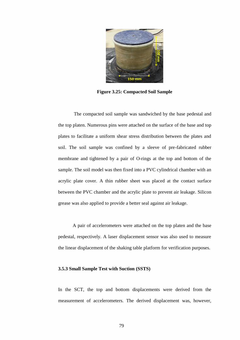
79

100 mm

150 mm

Figure 3.25: Compacted Soil Sample

The compacted soil sample was sandwiched by the base pedestal and

the top platen. Numerous pins were attached on the surface of the base and top

plates to facilitate a uniform shear stress distribution between the plates and

soil. The soil sample was confined by a sleeve of pre-fabricated rubber

membrane and tightened by a pair of O-rings at the top and bottom of the

sample. The soil model was then fixed into a PVC cylindrical chamber with an

acrylic plate cover. A thin rubber sheet was placed at the contact surface

between the PVC chamber and the acrylic plate to prevent air leakage. Silicon

grease was also applied to provide a better seal against air leakage.

A pair of accelerometers were attached on the top platen and the base

pedestal, respectively. A laser displacement sensor was also used to measure

the linear displacement of the shaking table platform for verification purposes.

3.5.3 Small Sample Test with Suction (SSTS)

In the SCT, the top and bottom displacements were derived from the

measurement of accelerometers. The derived displacement was, however,

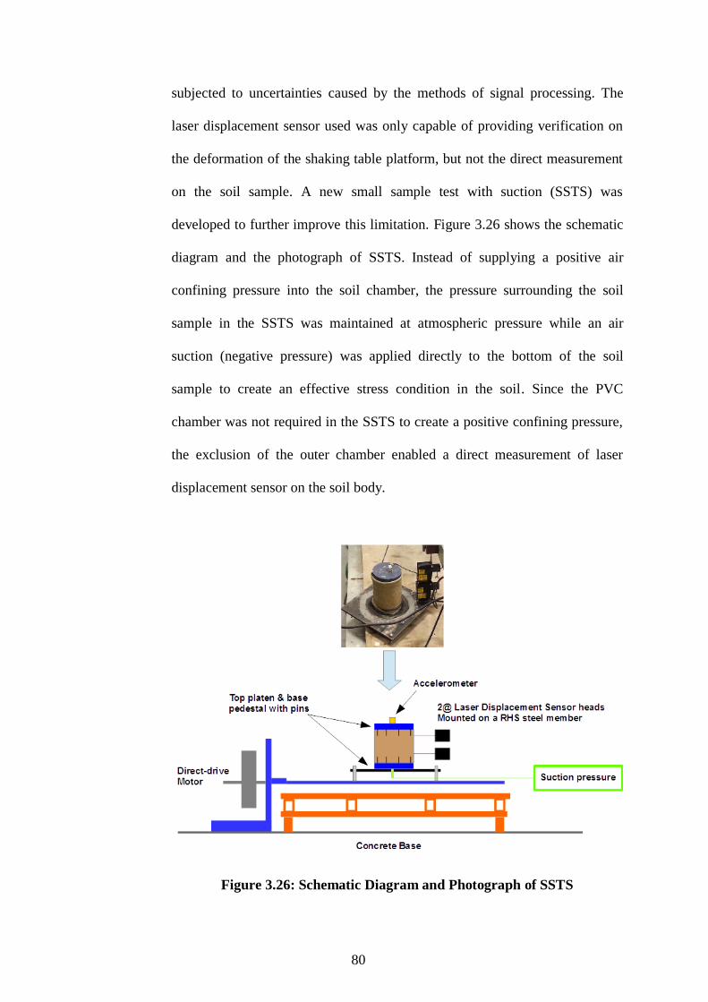
80

subjected to uncertainties caused by the methods of signal processing. The

laser displacement sensor used was only capable of providing verification on

the deformation of the shaking table platform, but not the direct measurement

on the soil sample. A new small sample test with suction (SSTS) was

developed to further improve this limitation. Figure 3.26 shows the schematic

diagram and the photograph of SSTS. Instead of supplying a positive air

confining pressure into the soil chamber, the pressure surrounding the soil

sample in the SSTS was maintained at atmospheric pressure while an air

suction (negative pressure) was applied directly to the bottom of the soil

sample to create an effective stress condition in the soil. Since the PVC

chamber was not required in the SSTS to create a positive confining pressure,

the exclusion of the outer chamber enabled a direct measurement of laser

displacement sensor on the soil body.

Figure 3.26: Schematic Diagram and Photograph of SSTS

81

Two laser displacement sensor heads were required in order to measure

the changes of shear strain profile with time. The suction (i.e. 50 kPa and 80

kPa) was supplied from a convum which was capable of converting a positive

air pressure into suction. It should be noted that the maximum suction that can

be produced was 80 kPa only as limited by the capacity of the convum.

3.6 Testing Parameters

Table 3.2 tabulates the testing parameters involved in the three laboratory

setups, namely LLSBT, SCT and SSTS. There were four main variables

investigated in the present study, i.e. shaking magnitude (i.e. input frequency

and input displacement), effective confining pressure, shear strain amplitude,

and soil type. The input motions applied for the large (LLSBT) and small

sample tests (SCT & SSTS) are summarized in Table 3.3 and Table 3.4,

respectively. It should be noted that different sets of shaking motions were

applied on the large and small sample tests. This was because the LLSBT was

first performed in this study, and hence the shaking motions covering a wide

range of frequencies and displacements were attempted in this preliminary

test. For the subsequent SCT and SSTS, it was intended to focus on the

shaking motions that could give favourable results based on the experience

from the LLSBT. Besides, the input shaking motions of the small sample test

were also constrained by the overall stability of the soil model during the

shaking test due to the slenderness and lighter selfweight of the samples

compared to the LLSBT.

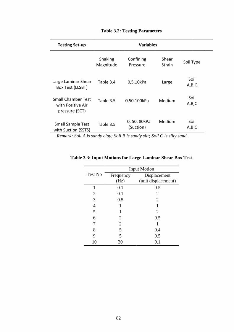
82

Table 3.2: Testing Parameters

Testing Set-up

Variables

Shaking Magnitude

Confining Pressure

Shear Strain

Soil Type

Large Laminar Shear Box Test (LLSBT)

Table 3.4 0,5,10kPa Large Soil

A,B,C

Small Chamber Test with Positive Air pressure (SCT)

Table 3.5

0,50,100kPa

Medium

Soil A,B,C

Small Sample Test with Suction (SSTS)

Table 3.5 0, 50, 80kPa

(Suction) Medium

Soil A,B,C

Remark: Soil A is sandy clay; Soil B is sandy silt; Soil C is silty sand.

Table 3.3: Input Motions for Large Laminar Shear Box Test

Test No

Input Motion

Frequency

(Hz)

Displacement

(unit displacement)

1 0.1 0.5

2 0.1 2

3 0.5 2

4 1 1

5 1 2

6 2 0.5

7 2 1

8 5 0.4

9 5 0.5

10 20 0.1

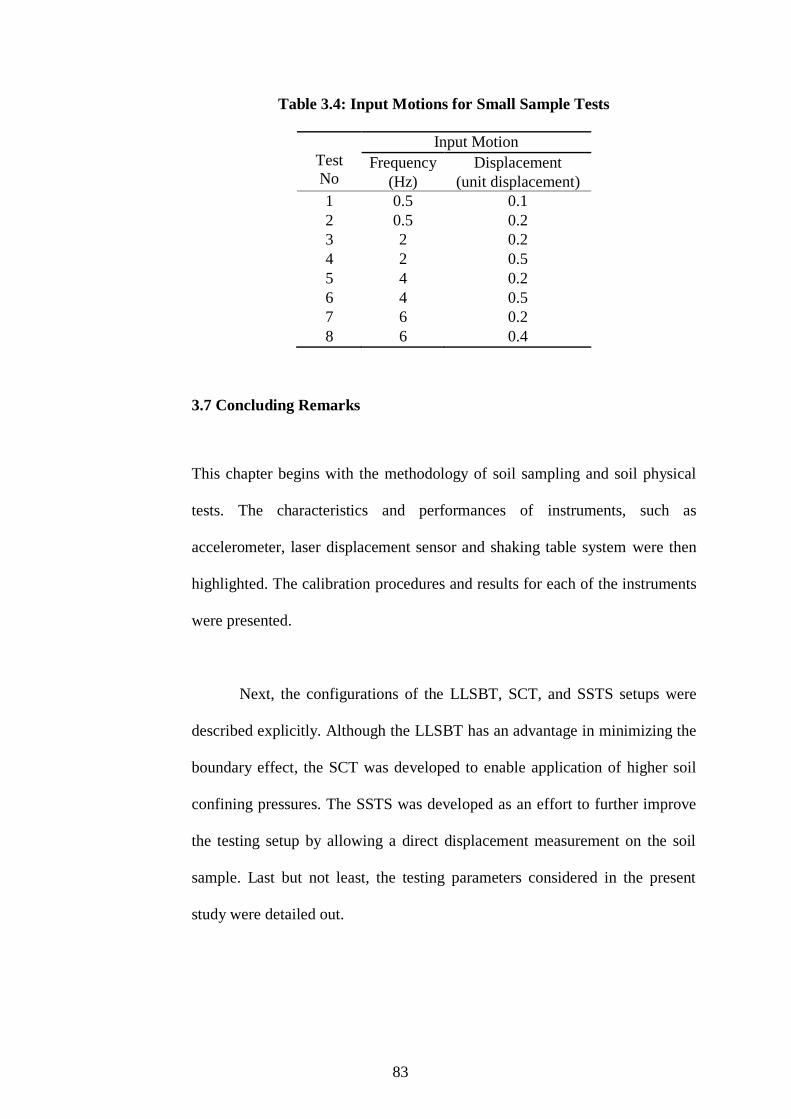
83

Table 3.4: Input Motions for Small Sample Tests

Test

No

Input Motion

Frequency Displacement

(Hz) (unit displacement)

1 0.5 0.1

2 0.5 0.2

3 2 0.2

4 2 0.5

5 4 0.2

6 4 0.5

7 6 0.2

8 6 0.4


This chapter begins with the methodology of soil sampling and soil physical

tests. The characteristics and performances of instruments, such as

accelerometer, laser displacement sensor and shaking table system were then

highlighted. The calibration procedures and results for each of the instruments

were presented.

Next, the configurations of the LLSBT, SCT, and SSTS setups were

described explicitly. Although the LLSBT has an advantage in minimizing the

boundary effect, the SCT was developed to enable application of higher soil

confining pressures. The SSTS was developed as an effort to further improve

the testing setup by allowing a direct displacement measurement on the soil

sample. Last but not least, the testing parameters considered in the present

study were detailed out.

CHAPTER 4

DATA PROCESSING

4.1 Introduction

Selecting an appropriate methodology in signal processing of acceleration data

is of importance to determine the dynamic properties of soils in a 1g shaking

table test. The dynamic properties are derived from the adjusted acceleration

and linear displacement data. This chapter provides a detailed approach on

choosing an appropriate data processing method for the present research.

4.2 Flowchart in Data Processing

Figure 4.1 depicts the flowchart of data processing. At the beginning, the raw

acceleration and linear displacement readings were measured and digitally

logged in a computer. The acceleration was measured by using an

accelerometer while the linear displacement was monitored by using a laser

displacement sensor. The entire records were subtracted from the mean of the

pre-event data. This procedure could correct the problem caused by DC bias

and it was widely defined as the zeroth-order baseline correction (Boore,

2001). Appropriate signal processing techniques were applied to the data in

order to remove the low and high frequency noises from the actual signal. Last

but not least, a number of parameters (i.e. shear stress, shear strain, secant

85

shear modulus and damping ratio) were computed through established theories

in the literature.

Figure 4.1: Flowchart in Data Processing

4.3 Data Processing Method

Figure 4.2 shows the measured acceleration profiles subjected to different

shaking frequencies (i.e. 2 Hz, 4 Hz, and 6 Hz). To eliminate the effect of DC

bias, the entire acceleration record was normalized with respect to the pre-

event data. Waveforms containing different frequency contents and

background noise effect can be observed in Figure 4.2 clearly.

Data Acquisition

Zeroth-order Baseline Correction

Signal Processing

(Baseline Correction and/or Filtering Method)

Data Analysis

(i.e shear stress, shear strain, shear modulus and damping ratio)

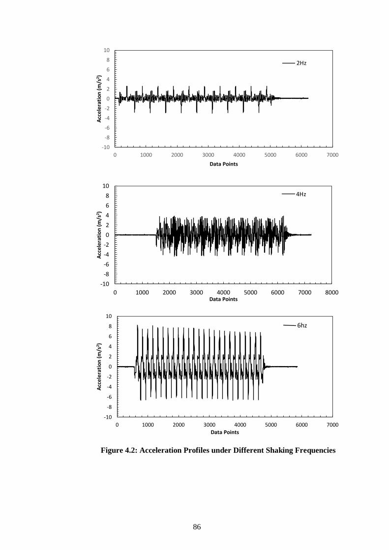
86

Figure 4.2: Acceleration Profiles under Different Shaking Frequencies

-10

-8

-6

-4

-2

0

2

4

6

8

10

0 1000 2000 3000 4000 5000 6000 7000

Acc

ele

rati

on

(m

/s2 )

Data Points

2Hz

-10

-8

-6

-4

-2

0

2

4

6

8

10

0 1000 2000 3000 4000 5000 6000 7000 8000

Acc

ele

rati

on

(m

/s2 )

Data Points

4Hz

-10

-8

-6

-4

-2

0

2

4

6

8

10

0 1000 2000 3000 4000 5000 6000 7000

Acc

ele

rati

on

(m

/s2 )

Data Points

6hz

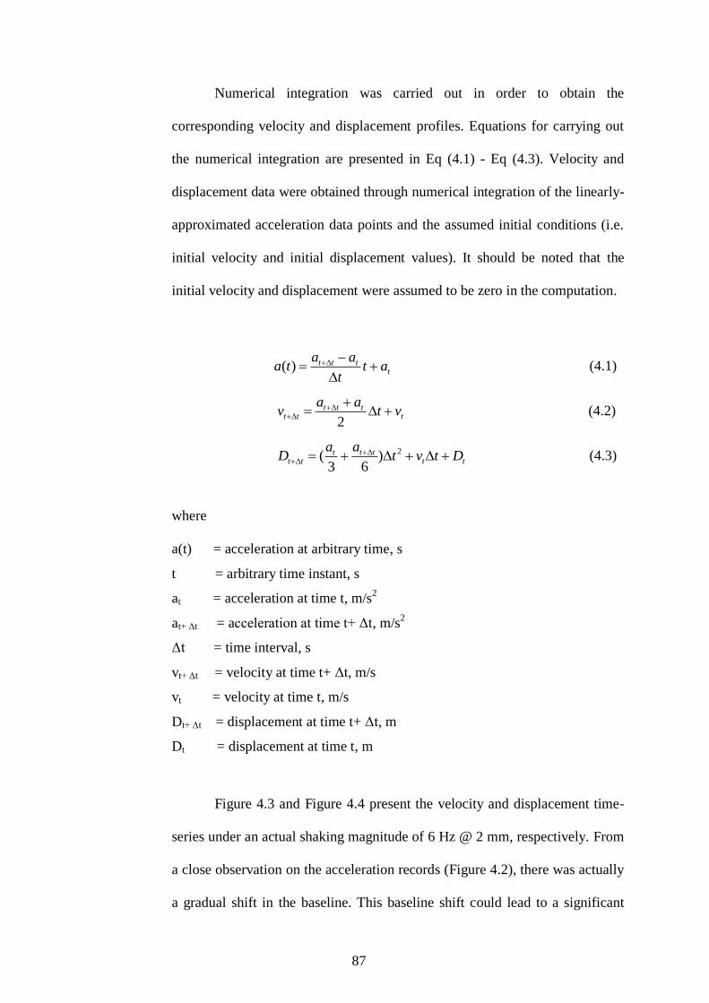
87

Numerical integration was carried out in order to obtain the

corresponding velocity and displacement profiles. Equations for carrying out

the numerical integration are presented in Eq (4.1) - Eq (4.3). Velocity and

displacement data were obtained through numerical integration of the linearly-

approximated acceleration data points and the assumed initial conditions (i.e.

initial velocity and initial displacement values). It should be noted that the

initial velocity and displacement were assumed to be zero in the computation.

tttt at

t

aata

)( (4.1)

tttt

tt vtaa

v

2 (4.2)

ttttt

tt Dtvtaa

D

2)63

( (4.3)

where

a(t) = acceleration at arbitrary time, s

t = arbitrary time instant, s

at = acceleration at time t, m/s2

at+ Δt = acceleration at time t+ Δt, m/s2

Δt = time interval, s

vt+ Δt = velocity at time t+ Δt, m/s

vt = velocity at time t, m/s

Dt+ Δt = displacement at time t+ Δt, m

Dt = displacement at time t, m

Figure 4.3 and Figure 4.4 present the velocity and displacement time-

series under an actual shaking magnitude of 6 Hz @ 2 mm, respectively. From

a close observation on the acceleration records (Figure 4.2), there was actually

a gradual shift in the baseline. This baseline shift could lead to a significant

mailto:[email protected]

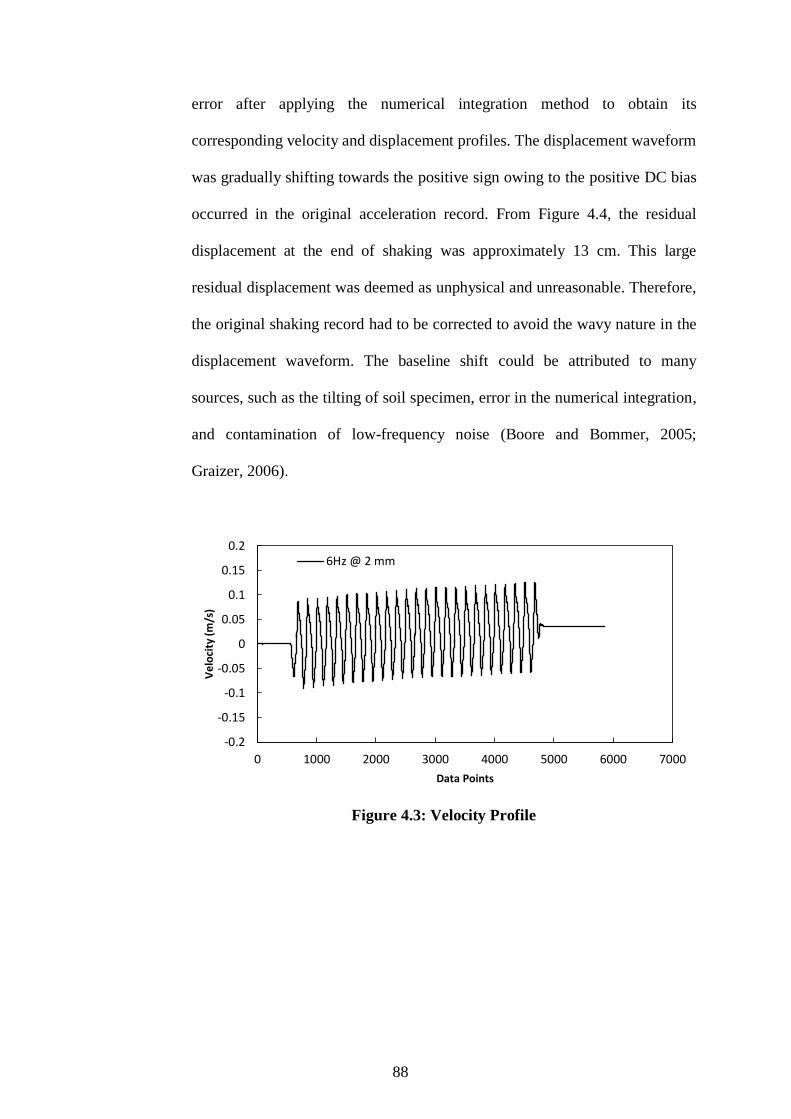
88

error after applying the numerical integration method to obtain its

corresponding velocity and displacement profiles. The displacement waveform

was gradually shifting towards the positive sign owing to the positive DC bias

occurred in the original acceleration record. From Figure 4.4, the residual

displacement at the end of shaking was approximately 13 cm. This large

residual displacement was deemed as unphysical and unreasonable. Therefore,

the original shaking record had to be corrected to avoid the wavy nature in the

displacement waveform. The baseline shift could be attributed to many

sources, such as the tilting of soil specimen, error in the numerical integration,

and contamination of low-frequency noise (Boore and Bommer, 2005;

Graizer, 2006).

Figure 4.3: Velocity Profile

-0.2

-0.15

-0.1

-0.05

0

0.05

0.1

0.15

0.2

0 1000 2000 3000 4000 5000 6000 7000

Ve

loci

ty (

m/s

)

Data Points

6Hz @ 2 mm

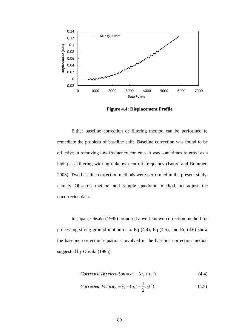
89

Figure 4.4: Displacement Profile

Either baseline correction or filtering method can be performed to

remediate the problem of baseline shift. Baseline correction was found to be

effective in removing low-frequency contents. It was sometimes referred as a

high-pass filtering with an unknown cut-off frequency (Boore and Bommer,

2005). Two baseline correction methods were performed in the present study,

namely Ohsaki’s method and simple quadratic method, to adjust the

uncorrected data.

In Japan, Ohsaki (1995) proposed a well-known correction method for

processing strong ground motion data. Eq (4.4), Eq (4.5), and Eq (4.6) show

the baseline correction equations involved in the baseline correction method

suggested by Ohsaki (1995).

)( 10 taaaonAcceleratiCorrected t (4.4)

)2

1( 2

10 tatavVelocityCorrected t (4.5)

-0.02

0

0.02

0.04

0.06

0.08

0.1

0.12

0.14

0 1000 2000 3000 4000 5000 6000 7000

Dis

pla

cem

en

t (m

m)

Data Points

6Hz @ 2 mm

90

)6

1

2

1( 3

1

2

0 tataDntDisplacemeCorrected t (4.6)

where

at = acceleration, m/s2

vt = velocity, m/s

Dt = displacement, m

a0, a1 = coefficients

t = time, s

The coefficients of the above equations can be computed based on the

assumptions that velocity will eventually become zero and there is a

reasonable residual displacement at the end of each shaking test. By knowing

the coefficients (i.e. a0 and a1), the equations for baseline correction can be

formed. It follows that the corrected acceleration, velocity and displacement

time-series can be obtained. In the present study, the computation of baseline

correction by Ohsaki (1995)’s method was performed with the aid of a coded

programming language, FORTRAN.

The simple quadratic method was processed by subtracting the entire

acceleration record from a quadratic least-square fitting line prior to the

numerical integration. This approach is widely used in the commercial data

processing programs, i.e. SeismoSignal. The simple quadratic baseline

correction method as adopted in SeismoSignal consists of the following

procedures: (1) determining a quadratic best-fit curve that fits the uncorrected

acceleration time-series through a regression analysis (i.e. quadratic least-

squares fitting), (2) subtracting the original acceleration record from the

established quadratic best-fit function, (3) undertaking numerical integration

91

to determine the velocity and displacement time-series. It is worth mentioning

that the approach adopted in SeismoSignal is not conceptually identical to the

baseline correction methods reported by Boore (2001). Boore (2001) first

identified the step changes in velocity trace and applied a linear or polynomial

best-fit to the velocity record. The raw acceleration data was then subtracted

from the derivative of velocity best-fit function.

Apart from the measurement of acceleration, the laser displacement

sensor was utilised as a direct displacement measurement device for

monitoring the linear displacement over time. During the test, a laser

displacement sensor was positioned near to the shaking table platform so that

the actual displacement at the base of the soil specimen could be monitored. It

was hoped that the actual displacement reading could be used to verify the

displacement derived from the accelerometer, which was mounted on the

shaking table. A suitable correction method could then be decided from the

comparison of the displacement data.

Figure 4.5 shows a series of displacement waveforms obtained from

the laser displacement sensor. The patterns of displacement waveforms

indicated that the shaking table machine can provide a fairly consistent cyclic

movement under different input frequencies and a certain input displacement.

In addition, Fourier Amplitude Spectra of the displacement movements for

LLSBT and SCT are plotted in Figure 4.6. Fast Fourier Transform was

involved in order to obtain the Fourier Amplitude Spectra. As inferred in the

Fourier Amplitude Spectra, the movement of the shaking table was inherently

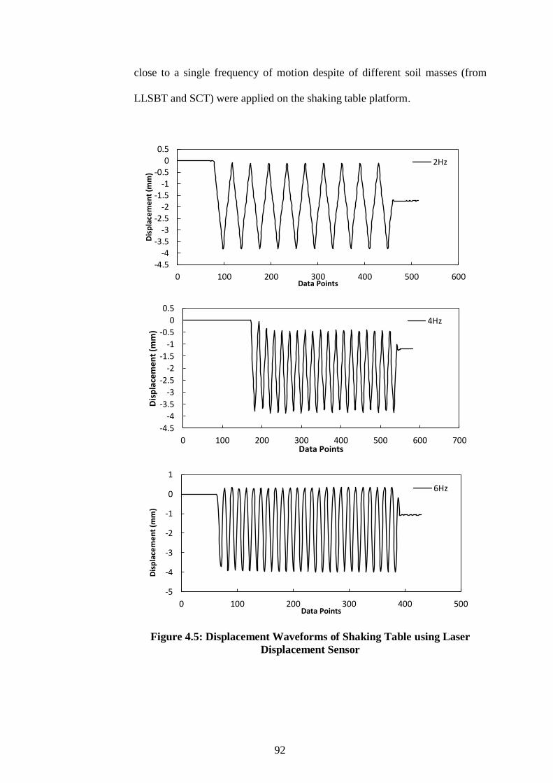
92

close to a single frequency of motion despite of different soil masses (from

LLSBT and SCT) were applied on the shaking table platform.

Figure 4.5: Displacement Waveforms of Shaking Table using Laser

Displacement Sensor

-4.5-4

-3.5-3

-2.5-2

-1.5-1

-0.50

0.5

0 100 200 300 400 500 600

Dis

pla

cem

en

t (m

m)

Data Points

2Hz

-4.5

-4

-3.5

-3

-2.5

-2

-1.5

-1

-0.5

0

0.5

0 100 200 300 400 500 600 700

Dis

pla

cem

ent

(mm

)

Data Points

4Hz

-5

-4

-3

-2

-1

0

1

0 100 200 300 400 500

Dis

pla

cem

en

t (m

m)

Data Points

6Hz

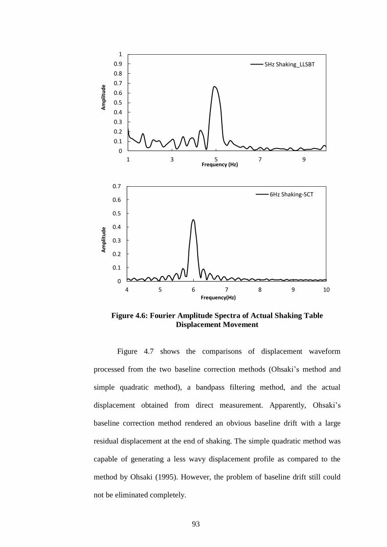
93

Figure 4.6: Fourier Amplitude Spectra of Actual Shaking Table

Displacement Movement

Figure 4.7 shows the comparisons of displacement waveform

processed from the two baseline correction methods (Ohsaki’s method and

simple quadratic method), a bandpass filtering method, and the actual

displacement obtained from direct measurement. Apparently, Ohsaki’s

baseline correction method rendered an obvious baseline drift with a large

residual displacement at the end of shaking. The simple quadratic method was

capable of generating a less wavy displacement profile as compared to the

method by Ohsaki (1995). However, the problem of baseline drift still could

not be eliminated completely.

0

0.1

0.2

0.3

0.4

0.5

0.6

0.7

0.8

0.9

1

1 3 5 7 9

Am

plit

ud

e

Frequency (Hz)

5Hz Shaking_LLSBT

0

0.1

0.2

0.3

0.4

0.5

0.6

0.7

4 5 6 7 8 9 10

Am

plit

ud

e

Frequency(Hz)

6Hz Shaking-SCT

94

Since the baseline-corrected record showed a somewhat wavy nature

of waveform, a high-pass or band-pass filtering was required to remove the

low-frequency and high-frequency unwanted signals. It should be noted that

the computed displacement traces from the accelerometer and the

measurements from the laser displacement sensor were not oscillated about the

same baseline. This was attributed to two standalone data logging systems

used when capturing the data.

Figure 4.7: Comparison of Three Correction Schemes and Laser

Displacement Measurement (6 Hz @ 2 mm)

Figure 4.8 shows the Fourier Amplitude Spectra of shaking table

records for the motion of laser sensor mounting system, ground motion, pre-

event motion, and post-event mean motion under a shaking magnitude of 6 Hz

@ 2 mm. It indicates that the shaking record was contaminated by low-

-0.008

-0.006

-0.004

-0.002

-1E-17

0.002

0.004

0.006

0.008

0.01

0 1 2 3 4 5 6 7

Dis

pla

cem

en

t (m

)

Time Index (s)

Simple Quadratic Baseline Correction

Osaki Baseline Correction

Laser Displacement Sensor

Bandpass Filtering


95

frequency and high-frequency noises. Boore and Bommer (2005) suggested an

approach of selecting a reasonable cut-off frequency in the low-pass filtering.

In the Fourier Amplitude Spectrum plot, the shaking record was compared

with its pre-event or post-event record. A higher frequency cut-off was

decided at a frequency where the signal record to noise ratio was below three.

Douglas and Boore (2010) also reported a detailed approach to choose a cut-

off frequency for high-pass filtering. Besides that, the frequency response of

the accelerometer was 50 Hz which should be taken into account when

selecting an appropriate cut-off frequency. However, the pre-event and post-

event records were unsuitable to be used as model noises when selecting the

cut-off frequencies, especially for the high-pass filtering. The acceleration

records, which were measured on the ground as well as on the laser sensor

mounting system, indicated that the shaking records were affected by the low-

frequency and high-frequency noises. Therefore, the displacement profiles

computed from the acceleration data were inaccurate owing to the

uncertainties in selecting an appropriate cut-off frequency.

In the present study, band-pass 4th-order Butterworth filtering was

attempted in this study. Bandpass filtering approach has been widely applied

in signal processing by many researchers (Brennan et al., 2005; Koga and

Matsuo, 1990). Herein, it was decided to set the amplitude difference between

the displacements obtained from filtering method and laser sensor

measurement to lie within 10 %, as a criterion when choosing a suitable

correction scheme. Slifka (2004) reported a similar criterion except that two

types of errors were introduced, namely standard error and peak error. From

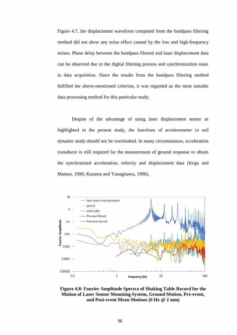
96

Figure 4.7, the displacement waveform computed from the bandpass filtering

method did not show any noise effect caused by the low and high-frequency

noises. Phase delay between the bandpass filtered and laser displacement data

can be observed due to the digital filtering process and synchronization issue

in data acquisition. Since the results from the bandpass filtering method

fulfilled the above-mentioned criterion, it was regarded as the most suitable

data processing method for this particular study.

Despite of the advantage of using laser displacement sensor as

highlighted in the present study, the functions of accelerometer in soil

dynamic study should not be overlooked. In many circumstances, acceleration

transducer is still required for the measurement of ground response to obtain

the synchronized acceleration, velocity and displacement data (Koga and

Matsuo, 1990; Kazama and Yanagisawa, 1996).

Figure 4.8: Fourier Amplitude Spectra of Shaking Table Record for the

Motion of Laser Sensor Mounting System, Ground Motion, Pre-event,

and Post-event Mean Motions (6 Hz @ 2 mm)


97


In conclusion, this chapter provides a detailed explanation on the approaches

adopted in selecting a suitable data processing method for the soil shaking

table tests. Various methods of data processing were examined and compared.

A laser displacement sensor was used to verify with the computed acceleration

data.

After conducting the shaking table test, the acceleration data was

processed and derived in order to obtain the linear displacement data. The

measured acceleration data was adjusted and numerically integrated. Since the

shaking signal was contaminated by both low and high-frequency noises under

the laboratory testing environment, the bandpass filtering method was finally

chosen as the signal processing method in the present study considering the

movement of the shaking table was pragmatically closed to a single frequency

of motion. The measured data was adjusted by making reference to the records

of laser displacement sensor. The baseline correction, although can eliminate

low-frequency noise, showed a wavy displacement profile containing high-

frequency noise. Despite of the benefits of using laser displacement sensor to

obtain the displacement waveform, accelerometer still served its function in

this study especially under conditions where placement of laser displacement

sensor was practically not viable.

CHAPTER 5

RESULT AND DISCUSSION

5.1 Introduction

This chapter presents the interpretation of experimental findings for the three

selected soils tested on the 1g shaking table in the laboratory. Two tropical

residual soils (i.e. Soil A and Soil B) and the sand mining trail (i.e. Soil C)

were tested by using three different types of experimental setup including

LLSBT, SCT, and SSTS. The measured acceleration data were processed

through the digital band-pass filtering and numerical integration methods.

Subsequently, shear strain profiles, shear stress profiles, and hysteresis loops

were obtained. Two important dynamic properties, namely secant shear

moduli and damping ratios, were determined from a series of hysteresis loops.

The results of dynamic properties were compared with the findings reported in

the literature. In addition, the effects of various parameters (e.g. confining

pressure, plasticity index, shear strain amplitude, and types of soil) on the soil

dynamic properties were investigated explicitly in the present study.

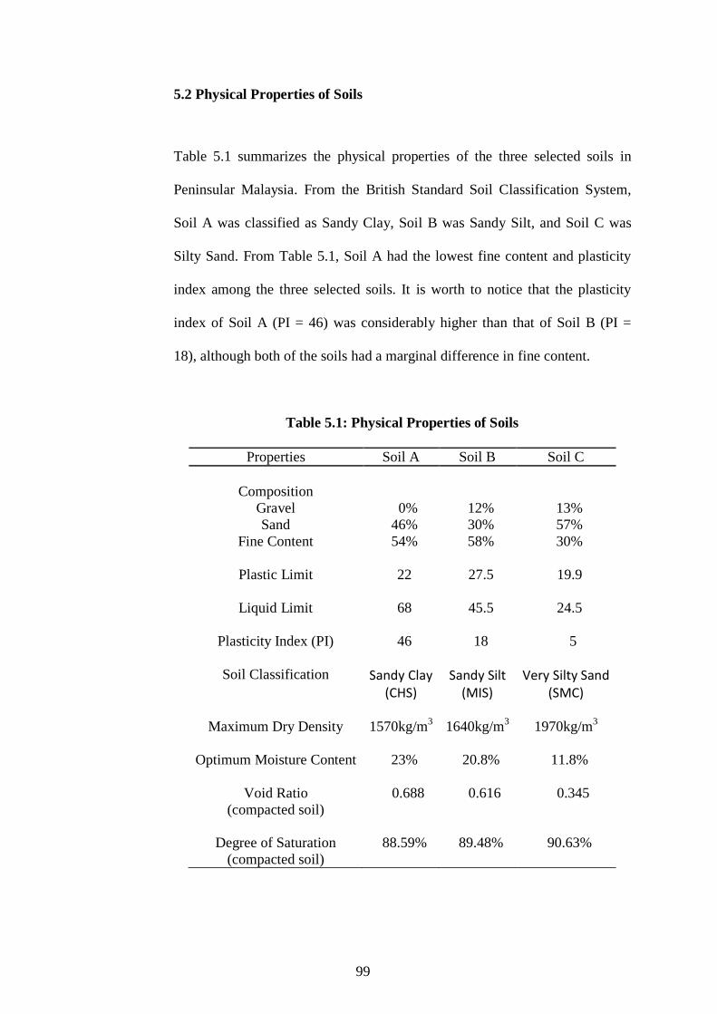
99

5.2 Physical Properties of Soils

Table 5.1 summarizes the physical properties of the three selected soils in

Peninsular Malaysia. From the British Standard Soil Classification System,

Soil A was classified as Sandy Clay, Soil B was Sandy Silt, and Soil C was

Silty Sand. From Table 5.1, Soil A had the lowest fine content and plasticity

index among the three selected soils. It is worth to notice that the plasticity

index of Soil A (PI = 46) was considerably higher than that of Soil B (PI =

18), although both of the soils had a marginal difference in fine content.

Table 5.1: Physical Properties of Soils

Properties Soil A Soil B Soil C

Composition

Gravel 0% 12% 13%

Sand 46% 30% 57%

Fine Content 54% 58% 30%

Plastic Limit

22 27.5 19.9

Liquid Limit

68 45.5 24.5

Plasticity Index (PI)

46 18 5

Soil Classification

Sandy Clay

(CHS)

Sandy Silt (MIS)

Very Silty Sand

(SMC)

Maximum Dry Density

1570kg/m3

1640kg/m3 1970kg/m

3

Optimum Moisture Content

23% 20.8% 11.8%

Void Ratio

(compacted soil)

0.688 0.616 0.345

Degree of Saturation

(compacted soil)

88.59% 89.48% 90.63%

100

5.3 Analysis of Experimental Data

This section covers the analyses of experimental data for LLSBT, SCT, and

SSTS, respectively. In the data processing stage, the uncorrected acceleration

data have been processed to eliminate the noise and baseline drift. The

adjusted acceleration and displacement data were used to analyse the dynamic

properties of soil i.e. secant shear modulus and damping ratio.

5.3.1 Analysis of Large Laminar Shear Box Test (LLSBT)

A shaking record of Soil A, with a shaking magnitude of 5 Hz @ 2.0 mm (i.e.

frequency of 5 Hz and single amplitude displacement of 2.0 mm) and

subjected to an overburden pressure of 10 kPa, was used as an example to

describe the results of data analysis using the LLSBT. Figure 5.1 depicts the

filtered acceleration profiles along the height of the soil model as well as on

the surcharge loading. At the base, the peak acceleration was approximately

0.2 g. Besides, the acceleration response on the surcharge loading (about 2.9

g) was significantly higher than the acceleration response in the soil model

(about 1.5 g – 2.0 g).

101

(a)

(b)

(c)

-5

-3

-1

1

3

5

0 1 2 3 4 5

Acc

eler

atio

n (

m/s

2)

Time (s)

Elevation: Base

-5

-3

-1

1

3

5

0 1 2 3 4 5

Acc

eler

atio

n (

m/s

2)

Time (s)

Elevation: 3.5cm

-5

-3

-1

1

3

5

0 1 2 3 4 5

Acc

eler

atio

n (

m/s

2)

Time (s)

Elevation: 7cm

102

(d)

(e)

(f)

Figure 5.1: Filtered Acceleration Profiles along the Height of Soil Model

-5

-3

-1

1

3

5

0 1 2 3 4 5

Acc

eler

atio

n (

m/s

2)

Time (s)

Elevation: 14cm

-5

-3

-1

1

3

5

0 1 2 3 4 5

Acc

eler

atio

n (

m/s

2)

Time (s)

Elevation: 21cm

-5

-3

-1

1

3

5

0 1 2 3 4 5

Acc

eler

atio

n (

m/s

2)

Time (s)

on Surchage Loading

103

Figure 5.2 shows the displacement profiles along the height of the soil

model. The filtered acceleration data (referred to Figure 5.1) were derived by

using the numerical integration method to obtain the displacement profiles.

The configuration of displacement profiles showed that the soil movements

were uniform and responded cyclically during the shaking table test. For this

example, the double amplitude of each displacement profile was nearly 0.004

m or 4 mm.

(a)

(b)

-0.003

-0.002

-0.001

0

0.001

0.002

0.003

0 1 2 3 4 5

Dis

pla

cem

ent

(m)

Time (s)

Elevation=Base

-0.003

-0.002

-0.001

0

0.001

0.002

0.003

0 1 2 3 4 5

Dis

pla

cem

ent

(m)

Time (s)

Elevation= 7cm

104

(c)

(d)

(e)

Figure 5.2: Filtered Displacement Profiles along the Height of Soil Model

-0.003

-0.002

-0.001

0

0.001

0.002

0.003

0 1 2 3 4 5

Dis

pla

cem

ent

(m)

Time (s)

Elevation= 10.5cm

-0.003

-0.002

-0.001

0

0.001

0.002

0.003

0 1 2 3 4 5

Dis

pla

cem

ent

(m)

Time (s)

Elevation= 14cm

-0.003

-0.002

-0.001

0

0.001

0.002

0.003

0 1 2 3 4 5

Dis

pla

cem

ent

(m)

Time (s)

Elevation= 21cm

105

Two monitoring points at different elevations along the same vertical

axis in the soil model were selected for verifying the occurrence of simple

shear deformation and the uniformity of shear strain profiles. Figure 5.3

depicts the displacement profiles at different elevations of the soil model

within a certain time frame. Figure 5.4 shows the displacement profiles at the

elevations of 3.5 cm and 10.5 cm, respectively. It shows that the displacement

at the elevation of 10.5 cm was greater than that of 3.5 cm and simple shear

deformation was distinguishable. The inertia shear stress applied on the top

surface of the soil at 10.5 cm was believed to have developed between the two

successive soil layers (3.5 cm – 10.5 cm) and that could represent the soil

condition below the ground surface. Besides, Figure 5.5 shows that the shear

strain profile at elevation interval of 3.5 cm – 10.5 cm was fairly uniform

compared to other intervals. Therefore the elevation interval of 3.5 cm – 10.5

cm was selected to determine the subsequent secant shear modulus and

damping ratio.

106

Figure 5.3: Displacement Profiles at Different Elevations

Figure 5.4: Comparison of Displacement Profiles between Elevations of

3.5 cm and 10.5 cm

-0.0025

-0.002

-0.0015

-0.001

-0.0005

0

0.0005

0.001

0.0015

0.002

0.0025

2.45 2.5 2.55 2.6 2.65 2.7 2.75 2.8

Dis

pla

cem

ent

(m)

Time (s)

Base

Elevation: 3.5cm

Elevation:7cm

Elevation: 10.5cm

Elevation: 14cm

Elevation: 17.5cm

Elevation: 21cm

-0.0025

-0.002

-0.0015

-0.001

-0.0005

0

0.0005

0.001

0.0015

0.002

0.0025

2 2.1 2.2 2.3 2.4 2.5 2.6

Dis

pla

cem

ent

(m)

Time (s)

Elevation=3.5cm

Elevation=10.5cm

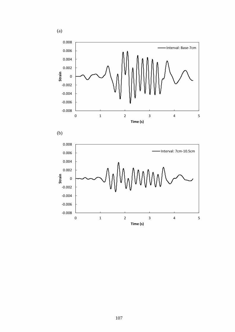
107

(a)

(b)

-0.008

-0.006

-0.004

-0.002

0

0.002

0.004

0.006

0.008

0 1 2 3 4 5

Stra

in

Time (s)

Interval: Base-7cm

-0.008

-0.006

-0.004

-0.002

0

0.002

0.004

0.006

0.008

0 1 2 3 4 5

Stra

in

Time (s)

Interval: 7cm-10.5cm

108

(c)

(d)

Figure 5.5: Shear Strain Profiles along Different Elevation Intervals of

Soil Model

The shear stress developed on the top surface of the elevation 10.5 cm

was computed by taking into account of the inertia shear stresses from the

overburden soil and the inertia shear stress induced by the surcharge loading

(Figure 5.6). The inertia shear stress of each soil layer is the integral product

-0.008

-0.006

-0.004

-0.002

0

0.002

0.004

0.006

0.008

0 1 2 3 4 5

Stra

in

Time (s)

Interval: 3.5cm-10.5cm

-0.008

-0.006

-0.004

-0.002

0

0.002

0.004

0.006

0.008

0 1 2 3 4 5

Stra

in

Time (s)

Interval: 7cm-21cm

109

of soil density and average acceleration developed in each of the soil layer

(Kazama et al., 1996).

Figure 5.6: Shear Stress Profile on the Top Surface at the Elevation 10.5

cm

Figure 5.7 shows a sample of single-cycle hysteresis loop to represent

the response of cyclic movement at the selected elevation. The enclosed loop

area represents the work done in the system and the slope indicates the shear

modulus of soil (Brennan et al., 2005).

-3

-2

-1

0

1

2

3

0 1 2 3 4 5

Stre

ss (

kPa)

Time (s)

Shear Stress on Soil Interval

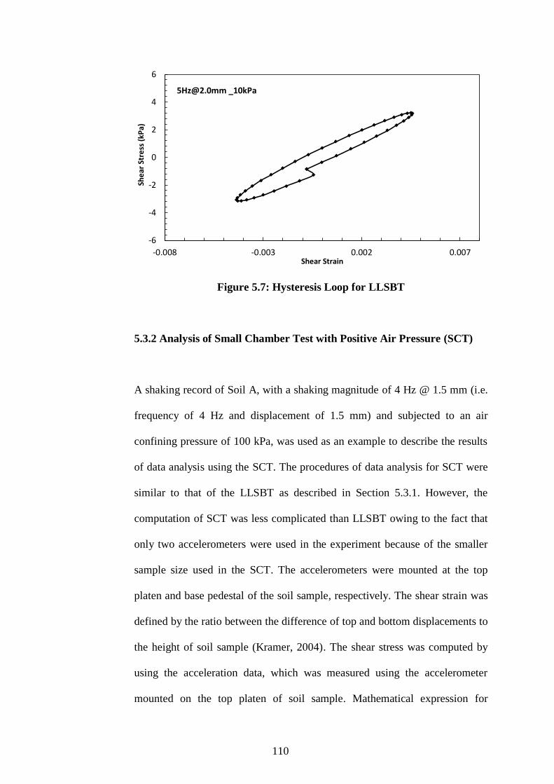
110

Figure 5.7: Hysteresis Loop for LLSBT

5.3.2 Analysis of Small Chamber Test with Positive Air Pressure (SCT)

A shaking record of Soil A, with a shaking magnitude of 4 Hz @ 1.5 mm (i.e.

frequency of 4 Hz and displacement of 1.5 mm) and subjected to an air

confining pressure of 100 kPa, was used as an example to describe the results

of data analysis using the SCT. The procedures of data analysis for SCT were

similar to that of the LLSBT as described in Section 5.3.1. However, the

computation of SCT was less complicated than LLSBT owing to the fact that

only two accelerometers were used in the experiment because of the smaller

sample size used in the SCT. The accelerometers were mounted at the top

platen and base pedestal of the soil sample, respectively. The shear strain was

defined by the ratio between the difference of top and bottom displacements to

the height of soil sample (Kramer, 2004). The shear stress was computed by

using the acceleration data, which was measured using the accelerometer

mounted on the top platen of soil sample. Mathematical expression for

-6

-4

-2

0

2

4

6

-0.008 -0.003 0.002 0.007

She

ar S

tre

ss (

kPa)

Shear Strain

[email protected] _10kPa

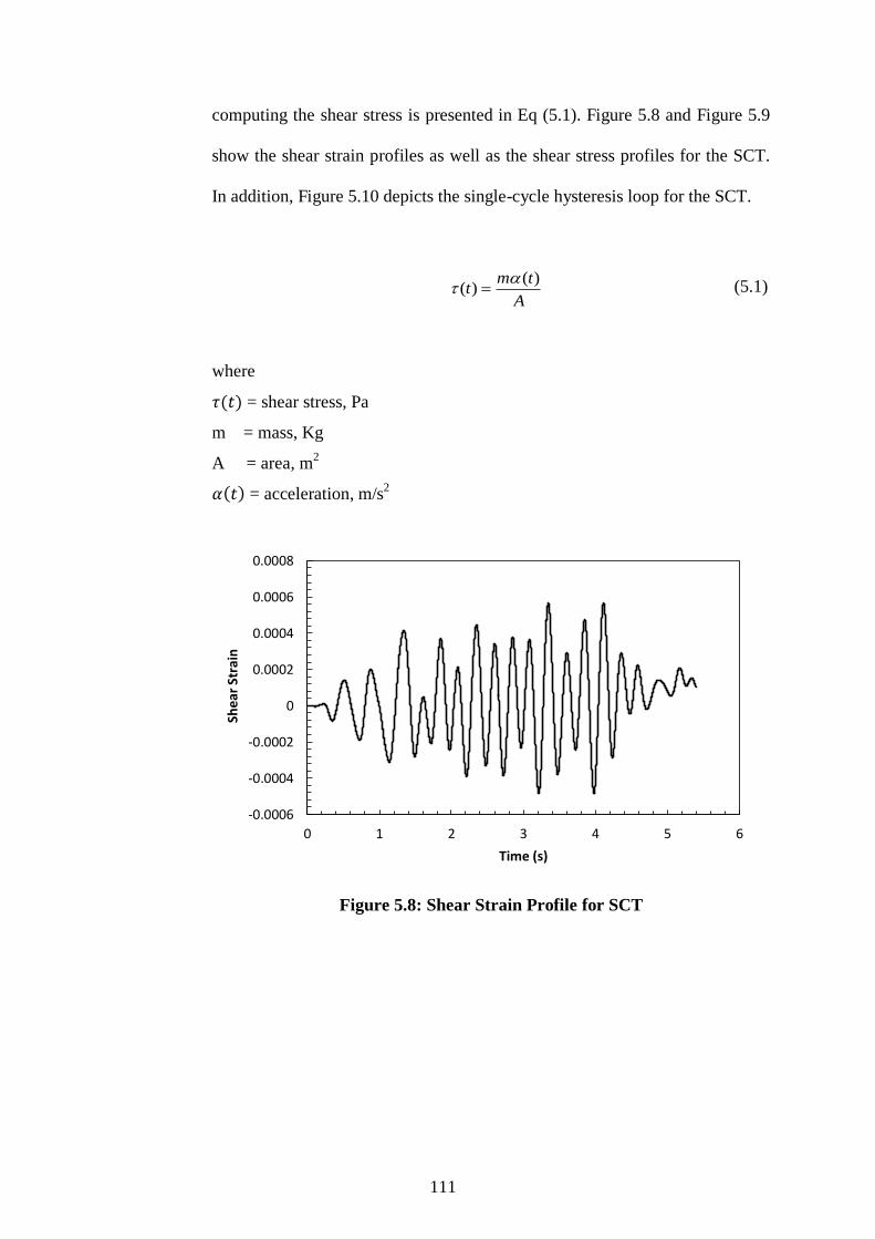
111

computing the shear stress is presented in Eq (5.1). Figure 5.8 and Figure 5.9

show the shear strain profiles as well as the shear stress profiles for the SCT.

In addition, Figure 5.10 depicts the single-cycle hysteresis loop for the SCT.

A

tmt

)()(

(5.1)

where

𝜏(𝑡) = shear stress, Pa

m = mass, Kg

A = area, m2

𝛼(𝑡) = acceleration, m/s2

Figure 5.8: Shear Strain Profile for SCT

-0.0006

-0.0004

-0.0002

0

0.0002

0.0004

0.0006

0.0008

0 1 2 3 4 5 6

Shea

r St

rain

Time (s)

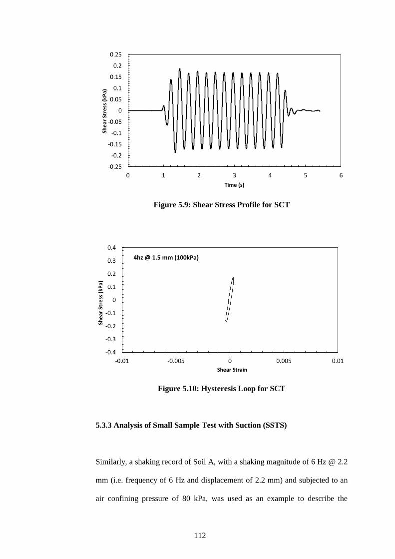
112

Figure 5.9: Shear Stress Profile for SCT

Figure 5.10: Hysteresis Loop for SCT

5.3.3 Analysis of Small Sample Test with Suction (SSTS)

Similarly, a shaking record of Soil A, with a shaking magnitude of 6 Hz @ 2.2

mm (i.e. frequency of 6 Hz and displacement of 2.2 mm) and subjected to an

air confining pressure of 80 kPa, was used as an example to describe the

-0.25

-0.2

-0.15

-0.1

-0.05

0

0.05

0.1

0.15

0.2

0.25

0 1 2 3 4 5 6

She

ar S

tre

ss (

kPa)

Time (s)

-0.4

-0.3

-0.2

-0.1

0

0.1

0.2

0.3

0.4

-0.01 -0.005 0 0.005 0.01

She

ar S

tre

ss (

kPa)

Shear Strain

4hz @ 1.5 mm (100kPa)

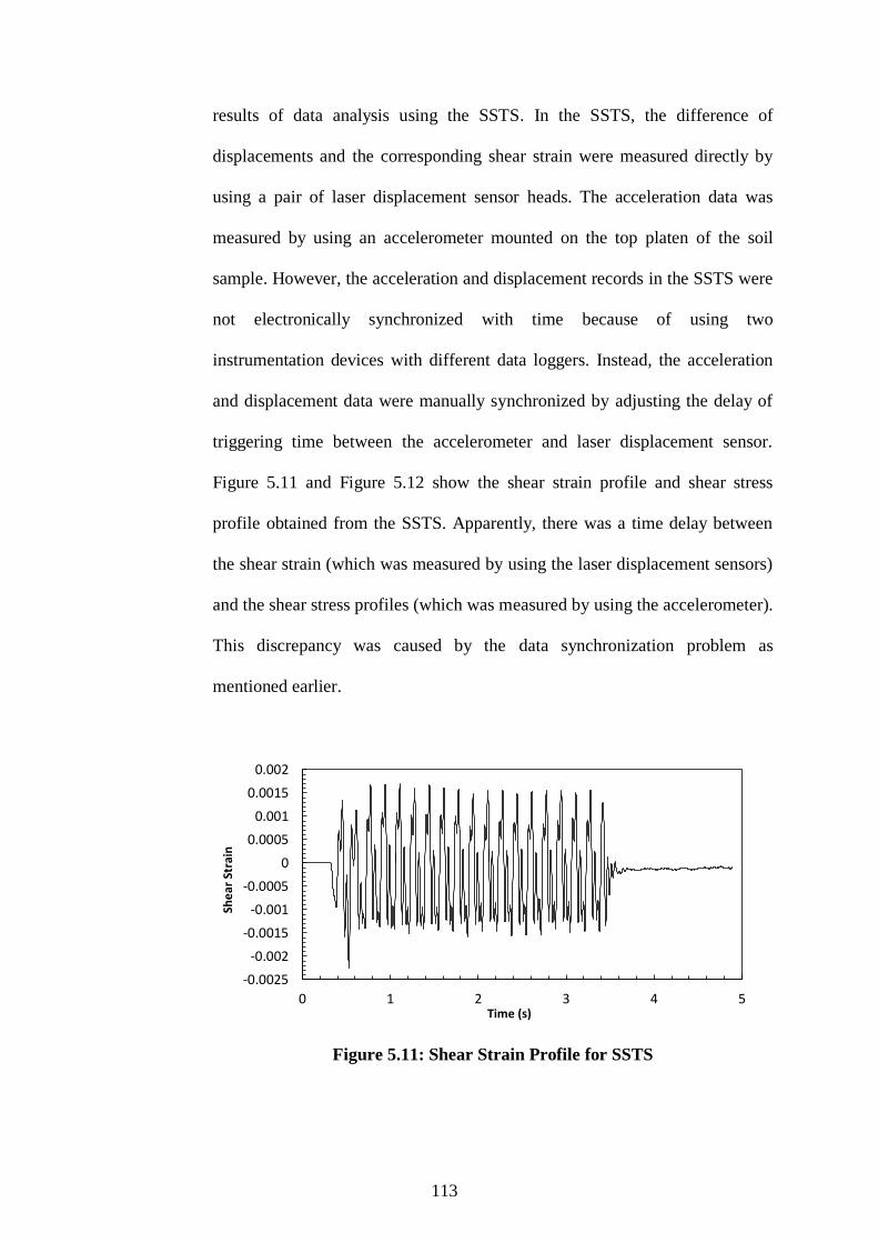
113

results of data analysis using the SSTS. In the SSTS, the difference of

displacements and the corresponding shear strain were measured directly by

using a pair of laser displacement sensor heads. The acceleration data was

measured by using an accelerometer mounted on the top platen of the soil

sample. However, the acceleration and displacement records in the SSTS were

not electronically synchronized with time because of using two

instrumentation devices with different data loggers. Instead, the acceleration

and displacement data were manually synchronized by adjusting the delay of

triggering time between the accelerometer and laser displacement sensor.

Figure 5.11 and Figure 5.12 show the shear strain profile and shear stress

profile obtained from the SSTS. Apparently, there was a time delay between

the shear strain (which was measured by using the laser displacement sensors)

and the shear stress profiles (which was measured by using the accelerometer).

This discrepancy was caused by the data synchronization problem as

mentioned earlier.

Figure 5.11: Shear Strain Profile for SSTS

-0.0025

-0.002

-0.0015

-0.001

-0.0005

0

0.0005

0.001

0.0015

0.002

0 1 2 3 4 5

She

ar S

trai

n

Time (s)

114

Figure 5.12: Shear Stress Profile for SSTS

In the previous chapter, the displacement profile of the shaking table

was found to be uniform and contained a dominant frequency of movement.

However, the trends of shear strain and stress profiles in the SSTS suggested

that the results were contaminated by noises with different frequency contents

(referred to Figure 5.11 and Figure 5.12). It was anticipated that the shear

strain and stress profiles in the SSTS were affected by the noises from the

supply of air suction pressure. Figure 5.13 shows a hysteresis loop for the

SSTS. The SSTS was unable to render a reasonable and consistent hysteresis

loop due to the problem of data synchronization and the noise effect.

-2

-1.5

-1

-0.5

0

0.5

1

1.5

2

0 1 2 3 4 5

She

ar S

tre

ss (

kPa)

Time (s)

115

Figure 5.13: Hysteresis Loop for SSTS

5.3.4 Summarizing the Results of Three Laboratory Setups

Table 5.2 summarizes the advantages and shortcomings of the LLSBT, SCT

and SSTS. Recommendations were put forward in Chapter 6 to improve the

test results of LLSBT, SCT and SSTS.

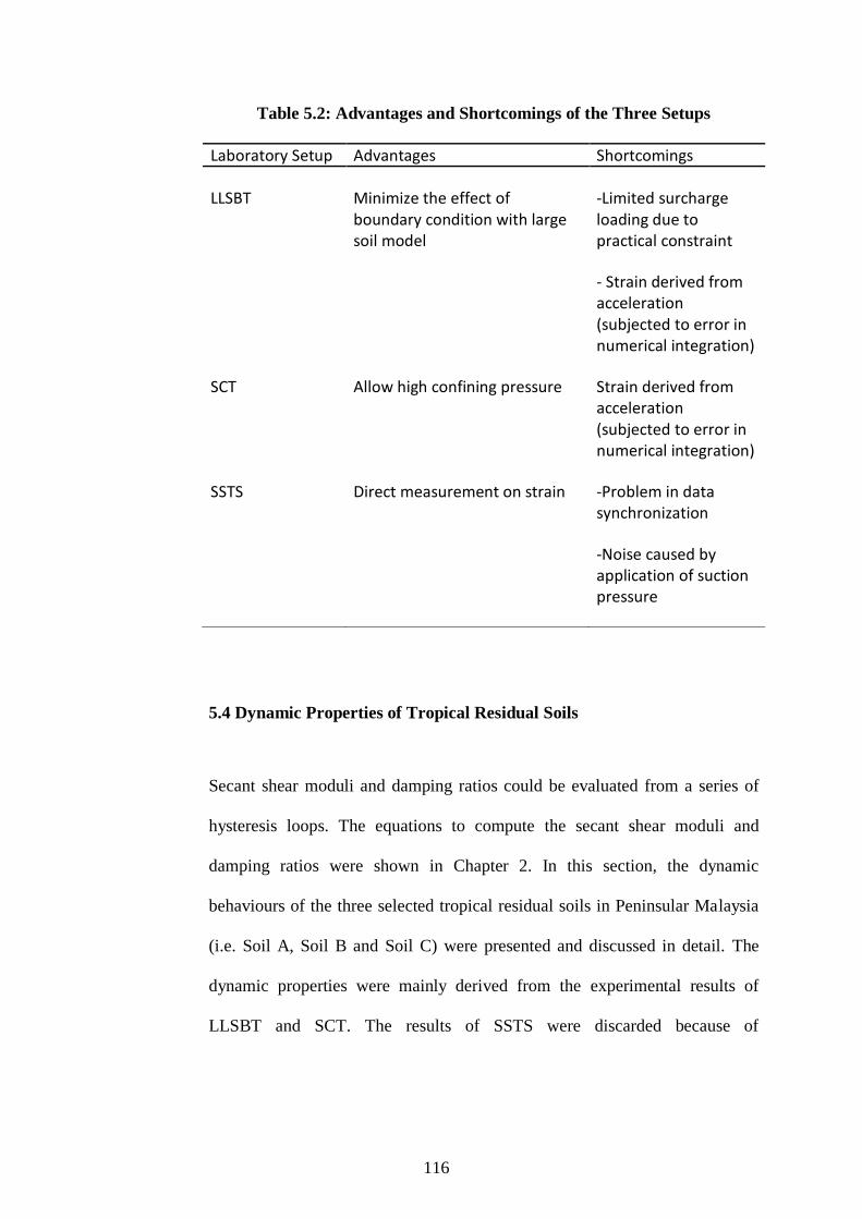
116

Table 5.2: Advantages and Shortcomings of the Three Setups

5.4 Dynamic Properties of Tropical Residual Soils

Secant shear moduli and damping ratios could be evaluated from a series of

hysteresis loops. The equations to compute the secant shear moduli and

damping ratios were shown in Chapter 2. In this section, the dynamic

behaviours of the three selected tropical residual soils in Peninsular Malaysia

(i.e. Soil A, Soil B and Soil C) were presented and discussed in detail. The

dynamic properties were mainly derived from the experimental results of

LLSBT and SCT. The results of SSTS were discarded because of

Laboratory Setup Advantages Shortcomings

LLSBT Minimize the effect of boundary condition with large soil model

-Limited surcharge loading due to practical constraint

- Strain derived from acceleration (subjected to error in numerical integration)

SCT Allow high confining pressure Strain derived from acceleration

(subjected to error in numerical integration)

SSTS Direct measurement on strain

-Problem in data synchronization

-Noise caused by application of suction pressure

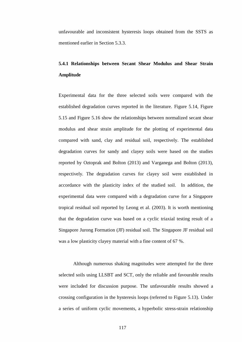
117

unfavourable and inconsistent hysteresis loops obtained from the SSTS as

mentioned earlier in Section 5.3.3.

5.4.1 Relationships between Secant Shear Modulus and Shear Strain

Amplitude

Experimental data for the three selected soils were compared with the

established degradation curves reported in the literature. Figure 5.14, Figure

5.15 and Figure 5.16 show the relationships between normalized secant shear

modulus and shear strain amplitude for the plotting of experimental data

compared with sand, clay and residual soil, respectively. The established

degradation curves for sandy and clayey soils were based on the studies

reported by Oztoprak and Bolton (2013) and Varganega and Bolton (2013),

respectively. The degradation curves for clayey soil were established in

accordance with the plasticity index of the studied soil. In addition, the

experimental data were compared with a degradation curve for a Singapore

tropical residual soil reported by Leong et al. (2003). It is worth mentioning

that the degradation curve was based on a cyclic triaxial testing result of a

Singapore Jurong Formation (JF) residual soil. The Singapore JF residual soil

was a low plasticity clayey material with a fine content of 67 %.

Although numerous shaking magnitudes were attempted for the three

selected soils using LLSBT and SCT, only the reliable and favourable results

were included for discussion purpose. The unfavourable results showed a

crossing configuration in the hysteresis loops (referred to Figure 5.13). Under

a series of uniform cyclic movements, a hyperbolic stress-strain relationship

118

was expected in a hysteresis loop (Hardin and Drnevich, 1972). For each type

of soil, there were in total four presentable data points each from the LLSBT

and SCT. When normalizing the secant shear modulus, the maximum shear

modulus was computed by using an empirical equation reported by Hardin and

Black (1968). The maximum shear moduli adopted in the present study ranged

from 10.6 MPa to 23.7 MPa depending on the soil type.

From Figure 5.15, the experimental data of Soil A (Sandy Clay) was

plotted below the lower bound of established curve for sand. It was also

plotted well below the established curve for clay. It should be noted that both

the established curves for sand and clay were developed from testing results of

pure sand and clay, respectively. It was anticipated that the mixture of sand

and clay in the natural tropical residual soil has altered their dynamic

properties significantly compared to the pure materials. For comparison with

residual soil, the experimental data of Soil A showed relatively good

agreement with the degradation curve of Singapore JF residual soil reported

by Leong et al. (2003). Similar trend as Soil A was also observed in Soil B

(Sandy Silt) as presented in Figure 5.16.

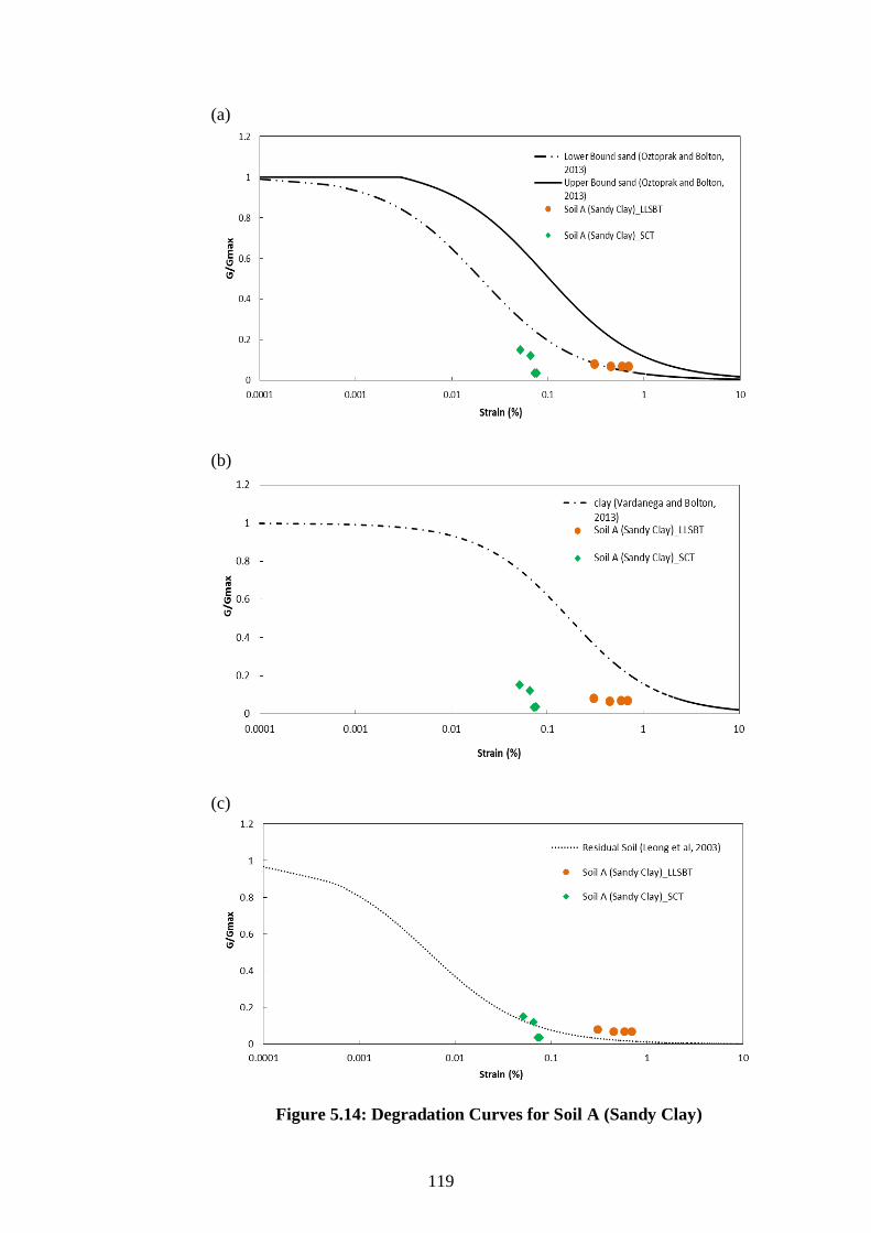
119

(a)

(b)

(c)

Figure 5.14: Degradation Curves for Soil A (Sandy Clay)

120

(a)

(b)

(c)

Figure 5.15: Degradation Curves for Soil B (Sandy Silt)

121

From the comparison between the experimental data and established

degradation curves, it can be inferred that the two selected tropical residual

soils (Soil A and Soil B) in Malaysia were unique and behaved neither as sand

nor clay. This observation was probably caused by the composition of sand-to-

fine content mixture, and the characteristics of parent rock formation of the

residual soils. This finding provoked further investigation on the dynamic

properties of residual soils in which a more explicit discussion will be

presented in the following Section 5.4.2.

From Figure 5.14, the experimental data of soil C (Silty Sand extracted

from sand mining trail) showed a relatively better fit to lower bound of sand

compared with Soil A and Soil B. This was because Soil C consists of

predominantly sandy material (i.e. content of coarse-grained material = 70 %).

However, the fine content in Soil C (i.e. 30 %) was believed to have played a

significant role on its dynamic properties. This was evidenced by some of the

mismatched data points below the lower bound of the established curve for

pure sand.

122

(a)

(b)

(c)

Figure 5.16: Degradation Curves for Soil C (Silty Sand)

123

5.4.2 Comparison of Present Data with Previous Findings of Residual

Soils

Figure 5.17 shows the comparison of experimental results in the present study

(residual Soil A and Soil B only) with the shear modulus of residual soils

reported from different parts of the world (Borden et al., 1996; Tou, 2003;

Leong et al., 2003; Tanaka and Lee, 2016). In general, shear moduli attenuate

with the increase of shear strain amplitude. The LLSBT and SCT were able to

facilitate soil movements from medium to large shear strain amplitude (i.e.

0.017 % to 1.48 %). SCT was able to facilitate soil movements with smaller

shear strain amplitude (i.e. 0.017 % - 0.077 %) as compared to the LLSBT (i.e.

0.077 % - 1.48 %).

Borden et al. (1996) investigated the dynamic properties of Piedmont

residual soil in North Carolina, United States. The compositions of Piedmont

residual soils ranged from silt to sand with different plasticity indexes. In their

study, Borden et al. (1996) focused mainly on the small-strain properties of

unsaturated soil samples using the resonant column and cyclic torsional shear

tests with the shear strain amplitude below 0.1 %. From Figure 5.17 it is

apparent that the shear moduli from the Piedmont residual soil were greater

than the experimental results of Soil A and Soil B. The discrepancy might be

attributed to the physical properties of residual soils and the characteristics of

parent rocks for different types of residual soil. The Piedmont residual soils

consisted of a wide spectrum of fine contents (in terms of silt and clay)

ranging from 10 % to 90 %, while the fine contents of Soil A and Soil B were

124

ranging from 54 % to 58 %. Besides, the degree of saturation of unsaturated

Piedmont residual soils were 39 % - 98 %, while the degree of saturation of

the residual soils in the present study were 88.6 % and 89.5 % for Soil A and

Soil B, respectively. From the literature, an unsaturated soil sample was

expected to have a higher stiffness than the saturated soil sample, and hence

the degree of saturation was an important parameter influencing the dynamic

properties of soils (Kramer, 2014). Soil A and Soil B were originated from the

sedimentary rocks whereas the Piedmont residual soil was originated from the

igneous and metamorphic rocks. In addition, the Piedmont soils are of sub-

tropic residual soils while the residual soils in the present study were

weathered under the tropical climate which was believed to have finer

particles under the intense weathering effect. From the foregoing, it can be

summarized that the dynamic properties of residual soil may be affected by

numerous factors including fine content, degree of saturation, characteristics

of parent rock, and weathering condition.

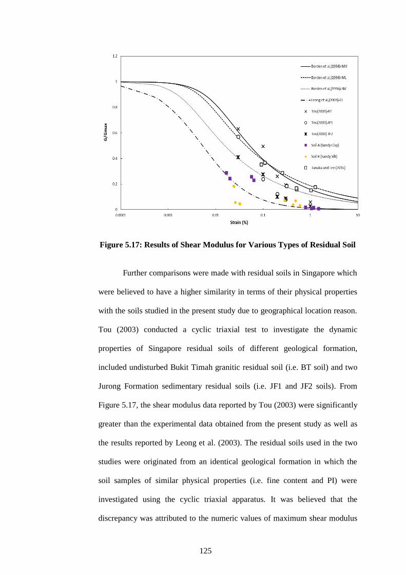
125

Figure 5.17: Results of Shear Modulus for Various Types of Residual Soil

Further comparisons were made with residual soils in Singapore which

were believed to have a higher similarity in terms of their physical properties

with the soils studied in the present study due to geographical location reason.

Tou (2003) conducted a cyclic triaxial test to investigate the dynamic

properties of Singapore residual soils of different geological formation,

included undisturbed Bukit Timah granitic residual soil (i.e. BT soil) and two

Jurong Formation sedimentary residual soils (i.e. JF1 and JF2 soils). From

Figure 5.17, the shear modulus data reported by Tou (2003) were significantly

greater than the experimental data obtained from the present study as well as

the results reported by Leong et al. (2003). The residual soils used in the two

studies were originated from an identical geological formation in which the

soil samples of similar physical properties (i.e. fine content and PI) were

investigated using the cyclic triaxial apparatus. It was believed that the

discrepancy was attributed to the numeric values of maximum shear modulus

126

obtained from either by experimental measurement (Tou, 2003) or by

estimation using empirical equations (Leong et al., 2003). The estimated

maximum shear moduli reported by Leong et al. (2003) were 64.7 MPa which

was significantly greater than the experimental maximum shear moduli of 28

MPa – 37 MPa reported by Tou (2003). In addition, it was reported that the

embedded uncertainties in interpreting the shear wave velocities could

significantly affect the accuracy of maximum shear moduli used for

normalizing the shear modulus data. Therefore, the importance of evaluating

the maximum shear modulus could not be overlooked in the experiment to

investigate the dynamic properties of soils. In the present study, the maximum

shear moduli for each of the soils were estimated in accordance with the

equation reported by Hardin and Black (1968), which was consistent with the

method adopted by Leong et al. (2003). As such, the shear modulus reported

in the present study showed good agreements with the degradation curves

proposed by Leong et al. (2003).

In addition, the results of the present study were further compared with

a previous study reported in Malaysia. Tanaka and Lee (2016) carried out a

series of 1g shaking table test on a compacted residual soil (Silty Sand of

Kenny Hill Formation from Alam Impian area). Prior to the shaking table test,

Tanaka and Lee (2016) conducted a pulse test to generate shear waves and

measure the shear wave velocity of the soil model. The maximum shear

modulus was estimated to be 5 MPa. From Figure 5.17, the shear modulus

data points reported by Tanaka and Lee (2016) agreed well with the

degradation curves of Borden et al. (1996) and Tou (2003), but they were

127

significantly greater than those reported by Leong et al. (2003) and the present

study. It is believed that the discrepancy was caused by the underestimation of

the maximum shear modulus compared with the typical values of maximum

shear modulus suggested in literature.

5.4.3 Effect of Plasticity Index and Confining Pressure on Shear Modulus

From the literature review, the effect of confining pressure on shear modulus

was significant in sandy soil, while the effect of plasticity index prevailed on

clayey soils. Figure 5.18 depicts the typical degradation curves for a sandy soil

under different levels of confining pressure (Oztoprak and Bolton, 2013). At

specific shear strain amplitude, the shear modulus increased with the

increasing confining pressure.

Figure 5.18: Effect of Confining Pressure on Shear Modulus for Sandy

Soil (Oztoprak and Bolton, 2013)

128

Figure 5.19 shows the typical degradation curves for a clayey soil with

different plasticity indexes (Vardanega and Bolton, 2013). At specific shear

strain amplitude, the shear modulus increased with the increasing plasticity

index.

Figure 5.19: Effect of Plasticity Index on Shear Modulus for Clayey Soil

(Vardanega and Bolton, 2013)

Figure 5.20 shows the experimental shear modulus obtained in the

present study for Soil A (Sandy Clay) and Soil B (Sandy Silt) with different

plasticity indexes. Apparently, the effect of plasticity index on the shear

modulus of soil was undistinguishable. The shear moduli for both soils were

plotted almost along an identical degradation curve despite of the fact that the

plasticity index of Soil A (PI = 46) was considerably higher than Soil B (PI =

18). It can thus be concluded that the studied residual soils in the present study

did not behave as the pure clayey soil even though the fine contents were

dominant in these soils.

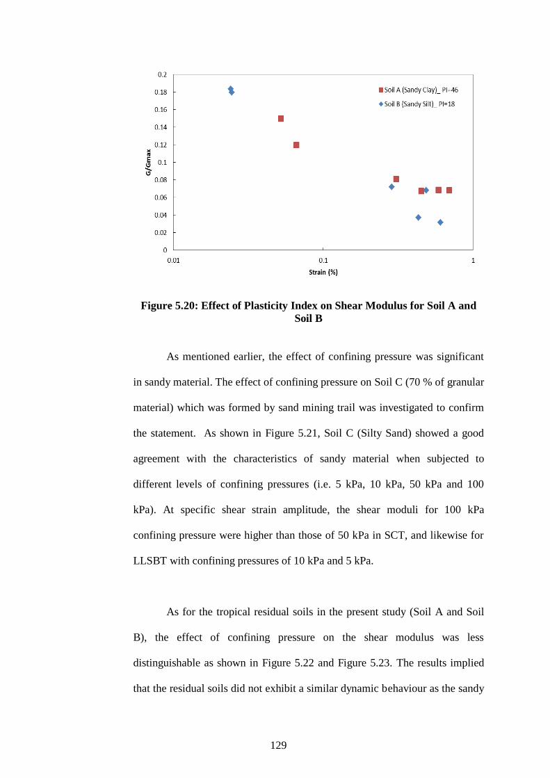
129

Figure 5.20: Effect of Plasticity Index on Shear Modulus for Soil A and

Soil B

As mentioned earlier, the effect of confining pressure was significant

in sandy material. The effect of confining pressure on Soil C (70 % of granular

material) which was formed by sand mining trail was investigated to confirm

the statement. As shown in Figure 5.21, Soil C (Silty Sand) showed a good

agreement with the characteristics of sandy material when subjected to

different levels of confining pressures (i.e. 5 kPa, 10 kPa, 50 kPa and 100

kPa). At specific shear strain amplitude, the shear moduli for 100 kPa

confining pressure were higher than those of 50 kPa in SCT, and likewise for

LLSBT with confining pressures of 10 kPa and 5 kPa.

As for the tropical residual soils in the present study (Soil A and Soil

B), the effect of confining pressure on the shear modulus was less

distinguishable as shown in Figure 5.22 and Figure 5.23. The results implied

that the residual soils did not exhibit a similar dynamic behaviour as the sandy

130

material. This was largely attributed to the presence of fine contents in the

studied residual soils (Soil A = 54 % and Soil B = 58 % of fine contents).

(a)

(b)

Figure 5.21: Effect of Confining Pressure on Shear Modulus (Soil C)

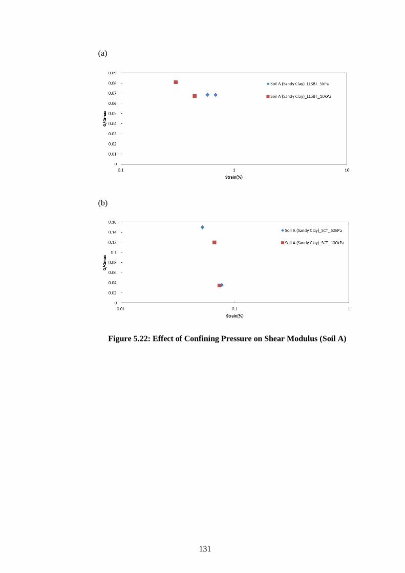
131

(a)

(b)

Figure 5.22: Effect of Confining Pressure on Shear Modulus (Soil A)

132

(a)

(b)

Figure 5.23: Effect of Confining Pressure on Shear Modulus (Soil B)

5.4.4 Relationship between Damping Ratio and Shear Strain Amplitude

Theoretically, damping ratio increases with the shear strain amplitude

(Ishibashi and Zhang, 1993). Figure 5.24 and Figure 5.25 show the

relationships between damping ratio and shear strain amplitude obtained from

the LLSBT and SCT, respectively. The experimental damping ratio data were

compared with the established damping ratio curves reported by Ishibashi and

Zhang (1993), which was obtained from statistical analysis on non-plastic

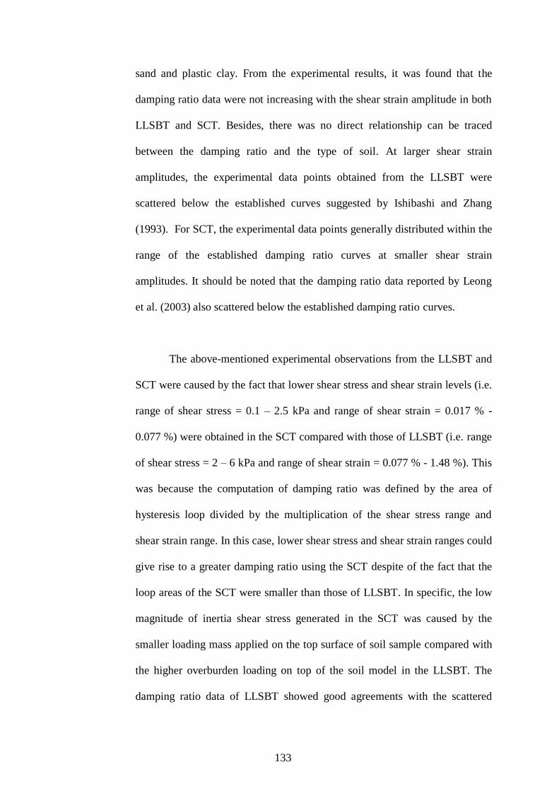
133

sand and plastic clay. From the experimental results, it was found that the

damping ratio data were not increasing with the shear strain amplitude in both

LLSBT and SCT. Besides, there was no direct relationship can be traced

between the damping ratio and the type of soil. At larger shear strain

amplitudes, the experimental data points obtained from the LLSBT were

scattered below the established curves suggested by Ishibashi and Zhang

(1993). For SCT, the experimental data points generally distributed within the

range of the established damping ratio curves at smaller shear strain

amplitudes. It should be noted that the damping ratio data reported by Leong

et al. (2003) also scattered below the established damping ratio curves.

The above-mentioned experimental observations from the LLSBT and

SCT were caused by the fact that lower shear stress and shear strain levels (i.e.

range of shear stress = 0.1 – 2.5 kPa and range of shear strain = 0.017 % -

0.077 %) were obtained in the SCT compared with those of LLSBT (i.e. range

of shear stress = 2 – 6 kPa and range of shear strain = 0.077 % - 1.48 %). This

was because the computation of damping ratio was defined by the area of

hysteresis loop divided by the multiplication of the shear stress range and

shear strain range. In this case, lower shear stress and shear strain ranges could

give rise to a greater damping ratio using the SCT despite of the fact that the

loop areas of the SCT were smaller than those of LLSBT. In specific, the low

magnitude of inertia shear stress generated in the SCT was caused by the

smaller loading mass applied on the top surface of soil sample compared with

the higher overburden loading on top of the soil model in the LLSBT. The

damping ratio data of LLSBT showed good agreements with the scattered

134

nature of data reported by Leong et al. (2003). It was unclear that this

observation was the result of sceptical reliability of the SCT setup or the

unique behaviours of tropical residual soils as opposing to the sand and clay

reported by Ishibashi and Zhang (1993). It is recommended that further studies

have to be conducted by using an alternative soil dynamic test (e.g. cyclic

triaxial test) to further investigate the damping ratio data at smaller shear strain

amplitudes. It is also worth mentioning that the frequencies of loading for the

LLSBT (i.e. 5 Hz) were slightly different to those applied in the SCT (i.e. 4

Hz – 6 Hz). This could give rise to a wider range of damping ratio data in the

SCT compared with those of LLSBT.

In addition, Brennan et al. (2005) reported that the damping ratio data

for a studied saturated sand (as shown in Figure 5.26) also scattered below the

established damping ratio curves reported by Ishibashi and Zhang (1993)

within the shear strain range of 0.1 % - 1 %.

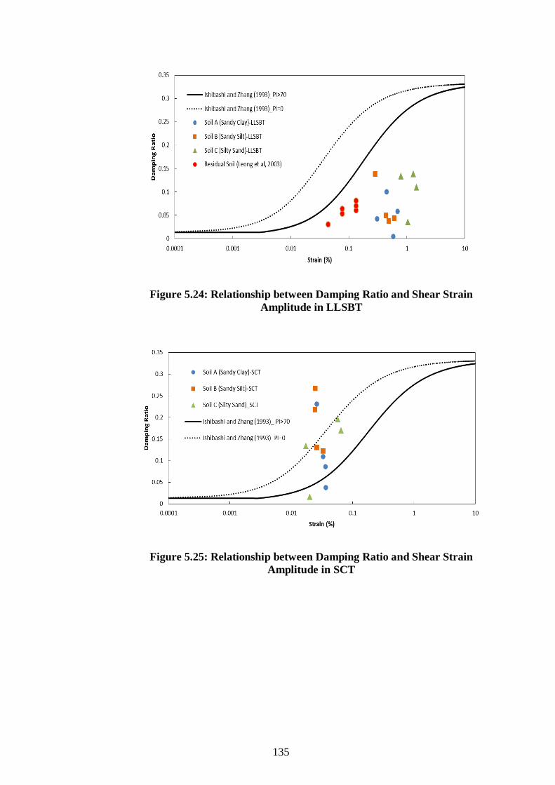
135

Figure 5.24: Relationship between Damping Ratio and Shear Strain

Amplitude in LLSBT


Amplitude in SCT

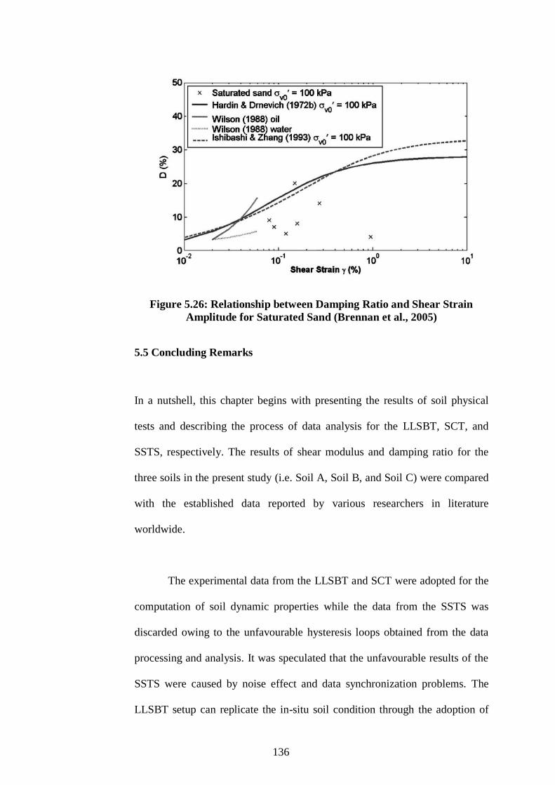
136


Amplitude for Saturated Sand (Brennan et al., 2005)


In a nutshell, this chapter begins with presenting the results of soil physical

tests and describing the process of data analysis for the LLSBT, SCT, and

SSTS, respectively. The results of shear modulus and damping ratio for the

three soils in the present study (i.e. Soil A, Soil B, and Soil C) were compared

with the established data reported by various researchers in literature

worldwide.

The experimental data from the LLSBT and SCT were adopted for the

computation of soil dynamic properties while the data from the SSTS was

discarded owing to the unfavourable hysteresis loops obtained from the data

processing and analysis. It was speculated that the unfavourable results of the

SSTS were caused by noise effect and data synchronization problems. The

LLSBT setup can replicate the in-situ soil condition through the adoption of

137

larger soil sample, which can minimize the effect of boundary in the soil

model. However, the LLSBT was not able to produce a high overburden

pressure on the soil model owing to the practical constraint in the laboratory.

Subsequently, the SCT was developed to impose higher confining pressures to

the soil sample in which the stress condition of soil below ground surface can

be reproduced. Despite of the fact that the LLSBT and SCT can be used to

examine the dynamic properties of soil under different testing conditions, the

data processing of the measured acceleration data was heavily subjected to the

uncertainties during numerical integration. It follows that the SSTS setup was

attempted to obtain the strain profile through direct displacement measurement

by using a pair of laser displacement sensor.

From the experimental results of LLSBT and SCT, the shear moduli of Soil C

(i.e. Silty Sand, with a fine content of 30 % only) was found to fit well with

the established degradation curves of sandy soil reported in literature. The

experimental shear moduli of two studied tropical residual soils, namely Soil

A and Soil B (i.e. Sandy Clay and Sandy Silt, with fine contents ranging from

54 % to 58 %) were found to be plotted below the established degradation

curves for sand and clay obtained from literature. It can be concluded that the

studied topical residual soils in Malaysia are unique and behave neither as

pure sand nor clay. The damping ratio results obtained from the experiment in

the present study were believed to have unique characteristics compared with

those of pure sand and clay as well. Further verification on the damping ratios

at smaller shear strain amplitudes is required for the tropical residual soils in

this study.

138

From the comparison between the experimental results in the present

study with the data reported by Borden and et al. (1996), Leong and et al.

(2003), Tou (2003), and Tanaka and Lee (2016), several factors were

identified to be influential on the dynamic properties of residual soils. These

include the degree of saturation, characteristics of parent rock, and the

weathering condition of the environment. Besides, the effects of confining

pressure and plasticity index on the studied tropical residual soils were found

to be undistinguishable. In the present study, the fine content was found to be

an influential parameter on the dynamic properties of selected tropical residual

soils in Malaysia.

CHAPTER 6

CONCLUSION

6.1 Summary

In the present study, two tropical residual soils (i.e. Soil A and Soil B) and a

sand mining trail (i.e. soil C) were sampled and tested on a 1g shaking table in

the laboratory. Three different models of experimental setup (i.e. LLSBT,

SCT, and SSTS) were developed to investigate the dynamic behaviours of

selected soils in the laboratory. In the 1g shaking table test, the measured

acceleration records were processed to obtain the shear strain and shear stress

data. The direct displacement measurement from the laser displacement sensor

was used to verify the shear strain derived from the measured acceleration

data. Finally, the results of secant shear modulus and damping ratio were

evaluated from the stress-strain relationships for the studied soils. The

experimental results of shear modulus and damping ratio were then compared

with the findings reported from previous studies.

6.2 Conclusions

In this study, three conclusions can be drawn in addressing the objectives set

forth in the Chapter 1:

140

i. To evaluate the performance of three different laboratory setups

on a 1g shaking table for soil dynamic testing:

In the present study, the experimental data of LLSBT and SCT were

used as the main raw data for interpreting dynamic properties of soils,

while the data of SSTS was discarded owing to the noise effect and the

problem of data synchronization occurred in the experiment. The

LLSBT setup has the advantage of replicating the in-situ soil condition

with a larger size of soil model in which the effect of boundary

condition can be minimized. However, it was impractical to apply a

high overburden pressure on the soil model of LLSBT. To overcome

this shortcoming, the setup of SCT was developed to apply higher

confining pressures to the soil sample in which the actual stress

condition of soil below the ground surface can be reproduced.

Although the LLSBT and SCT can be used to investigate the dynamic

properties of soil under various desired testing conditions, the

processed shear strain and shear stress data were subjected to

uncertainties in the data processing and numerical integration. The

setup of SSTS was attempted to measure the deformation of soil

sample directly by using a pair of laser displacement sensor. Medium

to large shear strain amplitudes of soil deformation can be obtained

from the present testing setups, i.e. LLSBT (i.e. 0.077 % - 1.48 %) and

SCT (i.e. 0.017 % - 0.077 %).

141

ii. To recommend the most suitable method of signal processing for

the shaking table test performed in this particular study:

Digital band-pass filtering is found to be the most suitable method in

this particular study. The integrated displacement profile matches

reasonably well with the laser displacement measurement.

iii. To investigate the dynamic properties of selected residual soils in

Malaysia:

From the experimental results of LLSBT and SCT, the shear moduli of

Soil C (i.e. Silty Sand, with a fine content of 30 % only) was found to

agree well with the established degradation curves of sand reported in

literature. The fine content in Soil C (i.e. 30 %) was anticipated to play

a significant role on the dynamic properties of soil. The experimental

shear moduli of two studied tropical residual soils, namely Soil A and

Soil B (i.e. Sandy Clay and Sandy Silt, with fine contents ranging from

54 % to 58 %) were found to be mismatched with and plotted below

the degradation curves for pure sand and clay reported in literature. It

can be concluded that the studied topical residual soils in Malaysia are

unique and behave neither as pure sand nor clay. This finding provokes

the need of further investigation on the dynamic properties of tropical

residual soils in Malaysia by using different types of soil dynamic

testing. The damping ratio results of the tropical residual soils in

Malaysia were unique compared with those of non-plastic sand and

plastic clay. Further verification on the damping ratios at smaller shear

strain amplitudes is required for the tropical residual soils. Comparing

142

the data reported by Borden et al. (1996) with the experimental data in

this study, degree of saturation, characteristics of parent rock, and the

weathering condition were found to be influential on the shear moduli

of tropical residual soils in Malaysia. In addition, fine content was

found to be an influential parameter on the dynamic properties of the

selected tropical residual soils in Malaysia.

6.3 Recommendation

There are several recommendations suggested for future improvement in this

area of research:

1. The sampling rate of acceleration data acquisition system was

suggested to be 0.1 ms when carrying out a pulse test for the soil

sample. By conducting the pulse test, shear wave velocity can be

measured and the maximum shear moduli at small shear strain

amplitudes can be obtained. The accelerometers should be aligned

parallel to each other prior to the generation of shear wave pulses by

using a sledge hammer.

2. Improvement has to be undertaken so as to solve the synchronization

problem when using the laser displacement sensor and accelerometer

simultaneously.

3. Further improvement has to be undertaken to examine the actual

movement of soil sample (i.e. direct measurements on the soil instead

143

of top platen and base pedestal). A pair of accelerometers, which are

separated by a certain height, can be installed on the circumferential

surface of the soil sample by using a thin metal probe. The laser beams

of the laser displacement sensor can be positioned at the same location

as the accelerometers. In addition, the actual movement of the soil

sample can be monitored and the computed shear strain from the

accelerometers can be compared with the measurement of laser

displacement sensor.

4. Since the achievable range of shear strain amplitudes is approximately

within the range from 0.01 % to 1 %, the application of 1g shaking

table itself cannot produce a wide range of shear strain amplitudes.

Different types of laboratory testing for investigating the dynamic

properties of soils have to be conducted, such as cyclic triaxial test,

hollow cylinder torsional shear test, bender element test, and etc.

5. It is suggested to carry out more tests on different types of tropical

residual soil to enrich the database of dynamic properties of tropical

residual soils.

144

REFERENCES

Adnan, A. and Suradi, S., 2008. Comparison on the effect of earthquake and wind

loads on the performance of reinforced concrete buildings. Proceedings of the

14th World Conference on Earthquake Engineering, 12 - 17 October 2008

Beijing, China.

Atkinson, J., 2007. The mechanics of soils and foundations, 2nd ed. Oxford: Taylor

and Francis.

Araei, A.A. and Towhata, I., 2014. Impact and cyclic shaking on loose sand properties

in laminar box using gap sensors. Soil Dynamics and Earthquake Engineering,

66 (2014), pp. 401 - 414.

Balendra, T. and Li, Z., 2008. Seismic hazard of Singapore and Malaysia. EJSE,

Special Issue: Earthquake Engineering in the low and moderate seismic

regions of South East Asia and Australia (2008), pp. 57 - 63.

Bjerrum, L. and Landva, A., 1966. Direct simple-shear tests on a Norwegian quick

clay. Geotechnique, 16 (1), pp. l - 20.

Boore, D.M., 2001. Effect of baseline corrections on displacements and response

spectra for several recordings of the 1999 Chi-Chi, Taiwan, earthquake.

Bulletin of the Seismological Society of America, 91 (5), pp. 1199 – 1211.

Boore, D.M. and Bommer, J.J., 2005. Processing of strong-motion accelerograms:

Needs, options and consequences. Soil Dynamics and Earthquake Engineering,

25 (2), pp. 93 – 115.

Borden, R.H., Shao, L.S. and Gupta, A., 1996. Dynamic properties of Piedmont

residual soils. Journal of Geotechnical Engineering, 122 (10), pp. 813 – 821.

Brennan, A.J., Thusyanthan, N.I. and Madabhushi, S.P.G., 2005. Evaluation of Shear

Modulus and Damping. Journal of Geotechnical and Geoenvironmental

Engineering, 131 (12), pp. 1488 – 1497.

BSI, 1990. British Standard 1377: Methods of test for soils for civil engineering

purposes. United Kingdom: BSI Group.

Budhu, M., 1983. Nonuniformities imposed by simple shear apparatus. Canadian

Geotechnical Journal, 21 (1), pp. 125 – 137.

Chiu, H.C., 1997. Stable baseline correction of digital strong-motion data, Bulletin of

the Seismological Society of America, 87 (4), pp. 932 – 944.

Dietz, M. and Wood, D.M., 2007. Shaking table evaluation of dynamic soil properties. Proceedings of the 4th International Conference on Earthquake Geotechnical

Engineering, 25 - 28 June 2007 Thessaloniki, Greece.

Douglas, J. and Boore, D.M., 2011. High-frequency filtering of strong-motion records.

Bulletin of Earthquake Engineering, 9 (2), pp. 395 – 409.

Dyvik, R., Berre, T., Lacasse, S. and Raadim, B., 1987. Comparison of truly

undrained and constant volume direct simple shear tests. Géotechnique, 37 (1),

pp. 3 – 10.

Elia, B.D., Lanzo, G. and Pagliaroli, A., 2003. Small-Strain Stiffness and Damping of

Soils in a Direct Simple Shear Device. Proc. 2003 Pacific Conference on

Earthquake Engineering, 13 – 15 February 2003 Christchurch, New Zealand.

Foo, K.Y., 1983. The Palaeozoic sedimentary rocks of Peninsular Malaysia-

stratigraphy and correlation. Proceedings of the Workshop on Stratigraphic

Correlation of Thailand and Malaysia, 8 – 10 September 1983 Haad Yai,

Thailand.

145

Graizer, V., 2006. Tilts in strong ground motion. Bulletin of the Seismological Society

of America, 96 (6), pp. 2090 – 2102.

Gue, S.S. and Wong, S.Y., 2009. Slope engineering design and construction practice

in Malaysia. CIE-IEM Joint Seminar on Geotechnical Engineering, 26 – 27

August 2009 Yilan, Taiwan.

Hardin, B.O. and Black, W.L., 1968. Vibration modulus of normally consolidated

clay. Journal of the Soil Mechanics and Foundations Division, 94 (2), pp. 353

– 369.

Hardin, B.O. and Drnevich, V.P., 1972. Shear modulus and damping in soils: design

equations and curves, Journal of the Soil Mechanics and Foundations Division,

98 (7), pp. 667 – 692.

Huat, B.B.K., Gue, S.S. and Faisal, H.A., 2004. Tropical residual soil engineering,

1st ed. London: Taylor and Francis.

Iai, S., 1988. Similitate for shaking table tests on soil-structure-fluid model in 1g

gravitational field. Report of the Port and Harbour Research Institute, 27 (3),

pp. 3 – 24.

Ishibashi, I. and Zhang, X., 1993. Unified dynamic shear moduli and damping ratios

of sand and clay. Soils and Foundations, 33 (1), pp. 182 – 191.

Ishihara, K. and Yamazaki, F., 1980. Cyclic simple shear tests on saturated sand in

multi-directional loading. Soils and Foundations, 20 (1), pp. 45 – 59.

Iwan, W.D., Moser, M.A. and Peng, C.Y., 1985. Some observations on strong-motion

earthquake measurement using a digital accelerograph. Bulletin of the

Seismological Society of America, 75 (5), pp. 1225 – 1246.

Iwasaki, T., Tatsuoka, F. and Takagi, Y., 1978. Shear Moduli of Sand under Cyclic

Torsional Shear Loading. Soils and Foundation, 18 (1), pp. 39 – 56.

Kazama, M., Toyota, H., Towhata, I. and Yanagisawa, E., 1996. Stress strain

relationship of sandy soils obtained from centrifuge shaking table tests.

Journal of JSCE, Geotechnical Engineering, Vol. 535 / III - 34, pp. 73 - 82.

(In Japanese)

Kazama, M. and Yanagisawa, E., 1996. Dynamic properties of soft clay directly

obtained from centrifuge shaking table test. Eleventh World Conference on

Earthquake Engineering, 23 – 28 June 1996 Acapulco, Mexico.

Koga, Y. and Matsuo, O., 1990. Shaking table tests of embankment resting on

liquefiable sandy ground. Soils and Foundations, 30 (4), pp. 162 – 174.

Kokusho, T., 1980. Cyclic Triaxial Test of Dynamic Soil Properties for wide strain

ranges. Soils and Foundations, 20 (2), pp. 45 – 60.

Kokusho, T., 2004. Nonlinear site response and strain-dependent soil properties.

Current Science, 87 (10), pp. 1363 – 1369.

Koo, K.K., Lim, J.X., Yang, C.L., Lee, M.L., Tanaka, Y. and Zhao, J.J., 2016.

Shaking table test on dynamic behaviours of tropical residual soils in Malaysia.

KSCE Journal of Civil Engineering, 21 (5), pp. 1735 - 1746.

Kramer, S.L., 2013. Geotechnical Earthquake Engineering, 1st ed. United Kingdom:

Pearson New International Edition.

Lanzo, G., Vucetic, M. and Doroudian, M., 1997. Reduction of Shear Modulus at

Small Strains in Simple Shear. Journal of Geotechnical and

Geoenvironmental Engineering, 123 (11), pp. 1035–1042.

Lee, V.W. and Trifunac, M.D., 1990. Automatic digitization and processing of

accelerograms using PC. Report CE 90 – 03, Department of Civil Engineering,

University of Southern California, United States.

146

Leong, E.C., Rahardjo, H. and Cheong, H.K., 2003. Stiffness-strain relationship of

Singapore residual soils. Proc. 2003 Pacific Conference on Earthquake

Engineering, 13 – 15 February 2003 Christchurch, New Zealand.

McCarthy, D.F., 1993. Essentials of soil mechanics: Basic geotechnics, 4th ed.

Englewood Cliffs, New Jersey: Regents/ Prentice Hall.

Mollova, G., 2007. Effects of digital filtering in data processing of seismic

acceleration records. Eurasip Journal on Advances in Signal Processing, 2007

(29502), pp. 1 - 9.

Mohd Rosaidi, C.A., 2001. Earthquake monitoring in Malaysia. Seismic Risk Seminar,

25 September 2001 Kuala Lumpur, Malaysia.

Nazri, F.M. and Alexander, N.A., 2012. Predicting the collapse potential of structures.

The 15th World Conference on Earthquake Engineering, 24 - 28 September

2012 Lisbon, Portugal.

Ooi, T.A., 1982. Malaysian soils and associated problems. Chapter 2, Geotechnical

Engineering Course, 22 March – 2 April 1982, University Malaya, Malaysia.

Ohsaki, Y., 1995. New introduction to spectrum analysis of earthquake ground

motion, Japan: Kajimashuppan (in Japanese).

Oztoprak, S. and Bolton, M.D., 2012. Stiffness of sands through a laboratory test

database. Géotechnique, 63 (1), pp. 54 – 70.

Piersol, A. and Paez, T., 2010. Harris' Shock and Vibration Handbook, 6th ed. Europe,

United States: McGraw-Hill Education.

Rahardjo, H., Aung, K.K., Leong, E.C. and Rezaur, R.B., 2004. Characteristics of

residual soils in Singapore as formed by weathering. Engineering Geology, 73

(2004), pp. 157 – 169.

Rahardjo, H., Lee, T.T., Leong, E.C. and Rezaur, R.B., 2005. Response of a residual

soil slope to rainfall. Canadian Geotechnical Journal, 42 (2), pp. 340 – 351.

Richardson, A.M. and Whitman, R.V., 1963. Effect of strain-rate upon undrained

shear resistance of a saturated remoulded fat clay. Geotechnique, 13 (4), pp.

310 – 324.

Seed, H.B. and Idriss, I.M., 1970. Soil moduli and damping factors for dynamic

response analyses. EERC report, EERC, California, United States.

Shakri, M.S. and Sanjery, K.A., 2015. Study potential earthquake threat in Peninsular

Malaysia. AENSI Journal, 9 (16), pp. 13 – 19.

Slifka, L.D., 2004. An Accelerometer Based Approach to Measuring Displacement of

a Vehicle Body. Master thesis, University of Michigan, Ann Arbor, United

States.

Sooria, S.Z., Sawada, S. and Goto, H., 2012. Proposal for seismic resistant design in

Malaysia: assessment of possible ground motions in Peninsular Malaysia.

Annuals of Disas. Prev. Res. Inst., Kyoto Univ., 30 September 2012 Kyoto,

Japan.

Taha, M. R., Hossain, M. K., & Mofiz, S. A., 2000. Effect of suction on the strength

of unsaturated soil. In Proceedings of Sessions of Geo-Denver 2000 -

Advances in Unsaturated Geotechnics, 5 – 8 August 2000 Denver, Colorado.

Tan, B.K. and Azwari Huslan Mohd., 2001. Physio-chemical properties of

carboneceauos shale soilsin the Yong Peng area, Johor. Geological Society of

Malaysia Annual Geological Conference, 10 October 2001 Pangkor Island,

Malaysia.

Tanaka, Y. and Lee, M.L., 2016. Laboratory study on dynamic properties of

compacted residual soil in Malaysia. Geotechnical Engineering Journal of the

SEAGS & AGSSEA, 47 (1), pp. 1 – 8.

147

Tou, J.H., 2003. Cyclic triaxial test apparatus for evaluating dynamic properties of

residual soils. Master Thesis, Nanyang Technological University, Singapore.

Tsai, C.C., Lin, W.C. and Chiou, J.S., 2016. Identification of dynamic properties

through shaking table tests on a large saturated sand specimen in a laminar

shear box. Soil Dynamics and Earthquake Engineering, 83 (2016), pp. 59 – 68.

Ueng, T.S., Chen, C.H. and Tsou, C.F., 2007. Preparation of large Mailiao silty sand

specimen for shaking table test. 4th International Conference on Earthquake

Geotechnical Engineering, 25 - 28 June 2007 Thessaloniki, Greece.

Vardanega, P.J. and Bolton, M., 2013. Stiffness of clays and silts : Normalizing shear

modulus and shear strain. Journal of Geotechnical and Geoenvironmental

Engineering. 139 (9), pp. 1575 – 1589.

Vucetic, M. and Dobry, R., 1991. Effect of soil plasticity on cyclic response. Journal

of Geotechnical Engineering, 117 (1), pp. 89 – 107.

Wijewickreme, D. and Vaid, Y.P., 2008. Experimental observations on the response

of loose sand under simultaneous increase in stress ratio and rotation of

principal stresses. Canadian Geotechnical Journal, 45 (5), pp. 597 – 610.

Xu, B.B., Nakai, K., Noda, T. and Takaine, T., 2013. A three dimensional soil-water

coupled FE analysis of hollow cylinder test concerning non-uniform

deformation. Soils and Foundations, 53 (6), pp. 923 – 936.

148

LIST OF PUBLICATIONS

1. Lim, J.X., Lee, M.L. and Tanaka, Y., 2017. Systematic Approaches for

Signal processing of soil shaking table test. The 6th

International

Conference of Euro Asia Civil Engineering Forum (EACEF-2017), 22-

25 August 2017 Seoul, South Korea. (Published)

2. Lim, J.X., Lee, M.L. and Tanaka, Y., 2017. Effect of fine content on

soil dynamic properties. Journal of Engineering Science and

Technology. (Conditionally accepted)

3. Lim, J.X., Lee, M.L. and Tanaka, Y., 2017. Investigation of soil

dynamic properties in Malaysia using 1g shaking table test with

different experimental setups. Geomechanics and Engineering.

(Under-reviewed)

Documents

EXPERIMENTAL STUDY ON DYNAMIC BEHAVIOUR OF TROPICAL RESIDUAL SOILS …eprints.utar.edu.my/2973/1/ESA-2018-1508242-1.pdf · 2018-08-06 · ii ABSTRACT EXPERIMENTAL STUDY ON DYNAMIC