Experimental study of the Thermal Behavior on Green Façades

Extended Abstract

Rita Ferreira Martins Gama Prazeres

July 2015

1

1. Introduction

The green façade development is justified with

the importance of buildings’ sustainability,

mainly in an urban environment where it is

crucial to have green spaces due to the high

construction density which leads to elevated air

temperatures. This fact is associated with the

buildings’ surface properties such as albedo,

the shading effect of leaves and the humidity

absorption that balance the concrete

domination. This solution also allows making

use of a vertical area that traditionally has no

other utilization, by bringing gardens to the

city.

This technique is more common in Northern

America and Northern Europe, where climate is

cooler, and this means that there aren’t many

experimental studies in a Mediterranean

climate. This paper’s main goal is to understand

the thermal behavior on green façades in the

referred climate, where mean temperatures

are higher in summer. In order to achieve that,

two case studies were monitored in Lisbon,

Portugal.

In parallel with this work, (Serpa, 2015) made

an energetic simulation of green façade also

related with the mentioned case studies.

This paper is divided into three distinct parts,

through six chapters. The first part focuses on

what has already been done in this field,

explaining the advantages, the different types

of construction and the conclusions of other

experimental studies. The second main part is

about the experimental phase, explaining what,

where and how the monitoring was done,

which instruments were used and also all the

result analyses of the two campaigns. Thirdly,

some conclusions were made about the

behavior of green façades.

2. State of the art

The origin of green façades lies in one of the

Seven Wonders of the Ancient World: the

Hanging Gardens of Babylon, built around 600

BC, by king Nebuchadnezzar II as a present to

his wife (Sousa, 2012). More recently, in the

late 20th century, vertical gardens appeared to

contrast the lack of green spaces in urban

areas. The pioneer of this modernized method

was Patrick Blanc, a botanist who made it

possible to build vertical gardens with no soil

involved, by placing the root plants in a

geotextile lining which absorbs the necessary

nutrients for the development of the plants,

while avoiding the spreading of pests that are

usually present on the ground.

2.1. Legislation

As far as the legislation is concerned, there are

a few laws and directives in some countries

that encourage the use of this solution or a

similar one. In Seattle, an ordinance requires

for buildings in process of construction to have

the equivalent of 30% of the surfaces vegetated

(Seattle Gov.) and, in New York City, a Bill

establishes green walls tax abatement for

certain properties (NY Bill). Also, in the

European Union, there is a project named

Green Tools for Urban Climate Adaptation that

intends to demonstrate and implement

technology to deal with climate adaptations in

urban areas and provide financial support.

2

2.2. Vertical greening systems

characterization

The expression “green façade” is associated

with all kinds of systems that cover walls with

vegetation. However, technically it is associated

to a specific system. In other words, there are

two distinct groups: the green façades and the

living wall system. The first one includes

climbing plants supported by cables or trellis or

attached directly to the building surface, where

the roots are on the ground or in plant boxes at

different heights. The living wall system refers

to a method that uses hydroponic culture

which allows plants to develop with no soil but

with all the needed nutrients. Instead of soil, it

uses geotextile layers to retain nutrients and

support the plants.

This paper will focus on living wall systems. Yet,

the expression “green façade” will cover all

types of vertical gardens.

2.3. Green façades benefits

By choosing this solution, the increase of green

spaces in cities is being promoted, and it may

help to improve air quality and reduce

temperature (Sheweka, et al., 2012).

Evapotranspiration and shading will also lessen

the heat that would be irradiated by a bare

façade. In addition, the layer of vegetation

protects the surface against UV’s so that the

materials such as painting, plaster, waterproof

membranes and others do not deteriorate

(Ottelé, 2011). Besides, it is also possible to

harvest rainwater for the watering system,

diminishing maintenance costs and relieving

the urban gutters. But the main profit analyzed

in this paper is the thermal behavior and how it

may help improve the internal temperatures of

a building.

2.4. Existing experimental

studies

There are a few studies that explore the

behavior of green façades and how they

influence the building. However, because there

aren’t many examples of this solution in a

Mediterranean climate, studies made on this

type of weather are scarce. (Olivieri, et al.,

2014) compares a green wall with a bare façade

and the results prove that vegetation lowers

the temperature experienced indoors. (Pérez,

et al., 2011) had similar results in the same

climate. (Eumorfopoulou, et al., 2009), also in a

similar climate, observed that the heat flux

transferred to the inside was lower than in a

bare façade.

Regarding the costs associated with this

solution, (Perini, et al., 2013) concluded that

they can vary from 400 up to 1200€/m2,

depending on the height of the building, but it

can lead to an energy saving of the air

conditioning within 40 to 60%.

3. Presenting the case studies

Both case studies were monitored during the

same time, in winter (from February 11 to

March 14) and summer (from June 16 to July

11), of 2014. The first one is a villa located in

downtown Lisbon (Figure 1) and the second

one is the entrance for a sound studio complex,

in Oeiras (Figure 2).

3

The equipments used were installed and

programmed to store all the needed

information, in the appropriate schedule, that

measured surface and ambient temperatures,

in- and outdoors, heat fluxes, solar radiation

and relative humidity.

Figure 1: Villa, in Travessa do Patrocínio

Figure 2: Entrance of the sound

studios complex, in Oeiras

The instruments used to obtain the required

information were Campbell data logger

(temperatures, fluxes and radiation),

DataTaker50 (temperatures and fluxes), Tinytag

and Rotronic (both relative humidity and

ambient temperature) in Travessa do

Patrocínio, while in Oeiras it was used the Data

Logger Delta T (temperatures, fluxes and

radiation) and also Rotronic and Tinytag.

The villa has simultaneously green and bare

façades, whereas the studio complex has not

only a wall but also a roof covered with

vegetation. In each case there is an air layer

between the building structure and the solution

itself. The thickness of that air layer is variable

on the villa (22 to 72 cm) and constant on the

studio entrance (5cm).

4. Experimental analysis –

Travessa do Patrocínio

Although the campaigns occurred almost at the

same time in both places, there were some

technical problems related to the energy

sources, sensors location or malfunction of the

equipments. Due to this, during winter, it was

not possible to register the vertical solar

radiation on the villa. Also, there were two

interruptions in the first case study. During

summer all the radiation was measured and

there was only one interruption due to a

technical issue. The sensors used to measure

temperature were type T thermocouples. The

heat flux sensor used was the Hukseflux HFP01,

a thermopile sensor with a measurement range

of ±2000W/m². To download the results, the

adapter VScom USB-COM-I was used to convert

RS422/485 port in USB port. Figure 3 presents

the sensors positioning scheme.

Figure 3: Representation of sensor positions in Travessa do Patrocínio

4

To understand the façade behavior, standard

days were chosen to represent the most

extreme conditions of the season. In other

words, during winter the standard days were

the coolest, the one with the lowest mean solar

radiation and the one with the highest mean

solar radiation, while in summer the standard

days were the hottest and the one with the

highest mean solar radiation.

Table 1: Mean values of horizontal solar radiation and exterior ambient temperature during winter

Date

Winter

2014

Ambient

mean

temperature

(°C)

Mean

solar

radiation

(W/m²)

Feb 21 12.1 102.9

Feb 22 12.2 103.1

Feb 23 12.6 113.6

Feb 24 12.7 102.8

Feb 25 13.2 68.5

Feb 26 13.6 89.8

Feb 27 13.4 52.1

Mar 3 13.7 76.7

Mar 4 13.3 79.4

Mar 5 14.5 101.2 RS- T-

Mar 6 14.1 120.7

Mar 7 17.0 128.6

Mar 8 18.0 94.0

Mar 9 15.3 35.0

Mar 10 16.6 104.1 RS+ T+

The standard days in winter were:

February 21 – Coolest day (12.1°C);

March 9 – Lowest mean solar radiation

day (35.0W/m²);

March 7 – Highest mean solar

radiation day (128.6W/m²).

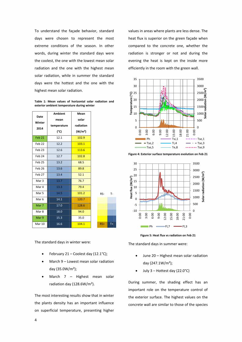
The most interesting results show that in winter

the plants density has an important influence

on superficial temperature, presenting higher

values in areas where plants are less dense. The

heat flux is superior on the green façade when

compared to the concrete one, whether the

radiation is stronger or not and during the

evening the heat is kept on the inside more

efficiently in the room with the green wall.

Figure 4: Exterior surface temperature evolution on Feb 21

Figure 5: Heat flux vs radiation on Feb 21

The standard days in summer were:

June 20 – Highest mean solar radiation

day (247.1W/m²);

July 3 – Hottest day (22.0°C)

During summer, the shading effect has an

important role on the temperature control of

the exterior surface. The highest values on the

concrete wall are similar to those of the species

0

500

1000

1500

2000

2500

3000

3500

0

5

10

15

20

25

30

35

0:0

0

3:0

0

6:0

0

9:0

0

12

:00

15

:00

18

:00

21

:00

0:0

0

Sola

r ra

dia

tio

n (

W/m

²)

Tem

per

atu

re (

°C)

Ph Tsi,1 Tse,1

Tse,2 Ti,4 Tse,3

Tse,5 Te,8 Tse,9

0

500

1000

1500

2000

2500

3000

3500

-10

-5

0

5

10

15

20

25

30

0:0

0

3:0

0

6:0

0

9:0

0

12

:00

15

:00

18

:00

21

:00

0:0

0

Sola

r ra

dia

tio

n (

W/m

²)

Hea

t fl

ux

(W/m

²)

Ph Fl,7 Fl,3

5

with the lowest density but all the others are

lower. Watering also decreases temperature

and evapotranspiration reflects on that same

effect. Interiorly, ambient temperature is near

the comfort values (REH, 2013) even with the

sun exposure through glass on the upper floor.

The room with the bare façade has no exposed

glazing.

Table 2: Mean values of horizontal solar radiation and exterior ambient temperature during summer

Data

Inverno

2014

Temperatura

média

ambiente

diária (°C)

Radiação

solar

média

diária

(W/m²)

17 Jun 20.2 65.8

18 Jun 20.5 142.7

19 Jun 20.5 237.2

20 Jun 20.5 247.1

21 Jun 20.2 226.3

22 Jun 19.7 194.6

23 Jun 18.5 162.2

24 Jun 20.5 205.8 RS- T-

3 Jul 22.0 189.9

4 Jul 21.8 204.7

5 Jul 21.7 205.9

6 Jul 20.5 124.0

7 Jul 20.2 199.6 RS+ T+

Figure 6: Solar radiation and surface temperature of B-B’ cross section on July 3

Some results of the hottest day are presented

in Figure 6, and Figure 7 shows the thermal

evolution of the green façade depending on

species.

Figure 7: Surface temperature evolution on June 20

Thermal conductivity test

In order to obtain an estimated value on the

thermal conductivity, an experimental test was

made with the instrument Isomet 2114.

Because it was not possible to obtain a sample

of the solution so that the test could be made

under controlled conditions, it was made in

situ, in Travessa do Patrocínio, in the winter

and before the watering system was activated.

Figure 8: Presentation (Fernandes, 2014) and installation of Isomet 2114

The obtained results are presented on Table 3.

0

500

1000

1500

2000

2500

3000

3500

0

5

10

15

20

25

30

35

40

0:0

0

3:0

0

6:0

0

9:0

0

12

:00

15

:00

18

:00

21

:00

0:0

0

Sola

r ra

dia

tio

n (

W/m

²)

Tem

per

atu

re (

°C)

Ph Pv Tse,3 Tsi,3 Tse,5 Tsi,5 Ti,4 Tse,6 Tsi,6 R

0

500

1000

1500

2000

2500

3000

3500

0

5

10

15

20

25

30

35

40

0:0

0

3:0

0

6:0

0

9:0

0

12

:00

15

:00

18

:00

21

:00

0:0

0

Sola

r ra

dia

tio

n (

W/m

²)

Te

mp

era

ture

(°C

)

Ph Pv Tse,1 Tse,2 Tse,3 Ti,4 Tse,5 Tse,9 Tsi,1 Te,8

6

Table 3: Obtained results

λ (W/m.°C) 0.2364

ϲρ x106 (J/m

3.°C) 0.3217

α (m2/s) 0.7349

Tmean (°C) 19.607

ΔT (°C) 9.8992

5. Experimental analysis –

Atlântico Blue Studios

As it was already mentioned, both case studies

campaigns occurred at the same time. During

winter, in Oeiras, it was not possible to register

the radiation values and there was also an

interruption on data acquisition due to a

battery fail. In summer campaign no issues

were registered, only the memory full on 3rd

and 4th of July. The sensors used were the

same as in the villa with an exception to one

thermocouple which was type K due to the

necessary length to get to the roof. So, Delta T

data logger had to be programmed depending

on the type of the thermocouples. Figure 9

presents the sensors positioning scheme.

The house has a pergola with retractable

shades that cover the monitored area when

open.

Figure 9: Representation of sensor positions in Oeiras

Table 4: Mean values of horizontal solar radiation and exterior ambient temperature during winter

Data

Inverno

2014

Temperatura

média

ambiente

diária (°C)

Radiação

solar

média

diária

(W/m²)

13 Fev 15.4 16.4

14 Fev 13.7 22.4

15 Fev 12.2 97.9

16 Fev 10.9 114.0

17 Fev 10.1 88.0

18 Fev 11.9 148.6

19 Fev 12.9 102.6

27 Fev 13.4 52.1

28 Fev 13.7 -

1 Mar 13.7 -

2 Mar 14.0 -

3 Mar 14.7 76.7

4 Mar 13.7 79.4

5 Mar 15.9 101.2

6 Mar 16.3 120.7

7 Mar 16.8 128.6

8 Mar 18.3 94.0 RS- T-

9 Mar 15.0 35.0

10 Mar 17.2 104.1

11 Mar 18.1 -

12 Mar 16.8 -

13 Mar 16.0 - RS+ T+

The standard days in winter were:

February 17 – Coolest day (10.1°C);

February 13 – Lowest mean solar

radiation day (16.4W/m²);

February 18 – Highest mean solar

radiation day (148.6W/m²).

7

Because of the existing air conditioning system

during the working days, it was interesting to

analyze the results that were registered on

Sundays, when the refrigeration equipment

was off. So, as the second coolest day was on a

Sunday (February 16th), it was also considered.

The 16th and 17th February had similar mean

temperatures. However, the temperature

range was higher on the 16th. Nevertheless, the

inner temperatures maintained a similar

behavior, proving that the solution is a good

insulation means. Through all days, the

difference between species is noticed even on

the internal surface, where denser vegetation

has lower temperatures. The roof is more

exposed to solar radiation, so those values are

higher.

Figure 10: Heat flux and surface temperatures on Feb 17

Figure 11: Heat flux and surface temperatures on Feb 16

Figure 10 and Figure 11 show that even with

the air conditioning operating, the temperature

felt on the interior surface almost does not

vary. The heat flux is positive, which means that

the energy is being stored inside, warming up

the ambient in the winter season. The 1pm

watering period is clear due to temperature

decreasing on the exterior, which increases

humidity and leads to a higher conductivity of

the geotextile that allows the heat to penetrate

through the wall.

Table 5: Mean values of horizontal solar radiation and exterior ambient temperature during summer

Data

Inverno

2014

Temperatura

média

ambiente

diária (°C)

Radiação

solar

média

diária

(W/m²)

18 Jun 20.9 289.3

19 Jun 19.4 344.9

20 Jun 19.7 347.6

21 Jun 20.2 288.7

22 Jun 19.1 158.7

23 Jun 18.5 205.8

24 Jun 20.1 246.1

25 Jun 21.3 285.1

26 Jun 21.4 347.5

27 Jun 21.5 351.9

28 Jun 21.7 223.4

29 Jun 20.7 352.5

30 Jun 21.6 351.8

1 Jul 22.2 218.4

2 Jul 22.7 262.5

5 Jul 21.7 300.7 RS- T-

6 Jul 20.6 169.4

7 Jul 20.3 319.8

8 Jul 21.3 328.0

9 Jul 22.9 326.7

10 Jul 23.3 327.2 RS+ T+

The standard days in summer were:

0

100

200

300

0

5

10

15

20

25

0:0

0

3:0

0

6:0

0

9:0

0

12

:00

15

:00

18

:00

21

:00

0:0

0

Hea

t fl

ux

(W/m

²)

Tem

per

atu

re (

°C)

Fl,1 Fl,2 Fl,4 Tsi,1 Tsi,2 Tsi,4 Tse,1 Tse,2 Tse,4

0

50

100

150

200

250

300

350

0

5

10

15

20

25

30

35

0:0

0

3:0

0

6:0

0

9:0

0

12

:00

15

:00

18

:00

21

:00

0:0

0

He

al f

lux

(W/m

²)

Te

mp

era

ture

(°C

)

Fl,1 Fl,2 Fl,4 Tsi,1 Tsi,2 Tsi,4 Tse,1 Tse,2 Tse,4

8

June 29 – Highest mean solar radiation

day (352.5W/m²);

July 10 – Hottest day (23.3°C)

Figure 12: Surface temperatures and solar radiation evolution on July 10

The huge difference between horizontal and

vertical radiation is related to the pergola that

shades the façade. It is important to

understand that the monitored façade area was

under the retractable shades so the radiation

results are reliable. Figure 12 shows an

accentuated increase of exterior surface

temperatures when radiation has higher values

but there is also a deceleration when watering

is activated (1pm) that also influences the

interior surface and the heat flux, proving that

evapotranspiration influences the thermal

behavior by slowing the heating process during

the hottest period of the day, allowing the

plants to humidify the surrounding

environment.

However, this effect is faster on this season, so

the geotextile conductivity doesn’t increase as

much as in winter, making it more difficult for

the heat to penetrate that layer.

Figure 13: Surface temperatures and heat flux on July 10

It is also interesting to observe the heat flux

variation that shows negative values during the

night, meaning that the heat is being released

to the outside (Figure 13). More important is

the peak value that never exceeds the values

registered during winter, evidencing the good

insulation behavior.

Once again, the roof values are superior to the

façade because of the higher solar exposition.

However, it is important to notice that the

temperature felt on the roof is almost the same

as the air temperature, enhancing the intrinsic

properties of the solution that attenuate the

building emissivity.

6. Conclusions

On both case studies there are not only

common but also distinct conclusions. The

differences remain on the construction such as

the air cavity thickness, the exposure of the

façade to radiation and the dimension and use

of the building.

The heat fluxes results show an optimistic

behavior depending on the season. In winter

the entrance values are higher than in summer

0

500

1000

1500

2000

2500

3000

3500

0

5

10

15

20

25

30

35

40

45

0:0

0

3:0

0

6:0

0

9:0

0

12

:00

15

:00

18

:00

21

:00

0:0

0

Sola

r ra

dia

tio

n (

W/m

²)

Tem

per

atu

re (

°C)

Ph Pv Tsi,1 Tsi,2 Tsi,4 Tse,1 Tse,2 Tse,4

-20

30

80

130

180

230

280

330

-15

-10

-5

0

5

10

15

0:0

0

3:0

0

6:0

0

9:0

0

12

:00

15

:00

18

:00

21

:00

0:0

0

Hea

t fl

ux

(W/m

²)

ΔT

(°C

)

Fl,2 Fl,1 Fl,4

Tse,2-Tsi,2 Tse,1-Tsi,1 Tse,4-Tsi,4

9

while the exit values are higher during the

night, in summer. This effect is due to

evapotranspiration which occurs after irrigation

and allows the plants to release water vapor.

This process is faster during heating season so

it leads to a better performance of the solution

by cooling down the surrounding environment

and insulating the building because the

humidity levels of the substrate are lower than

in winter, which means that thermal

conductivity is inferior in summer. Also

(Valadas, 2014) concluded the same on green

roofs.

The space between the vertical garden and the

structure of the building is thicker in Travessa

do Patrocínio and, according to ISO 13789, it is

considered a non used space with different

thermal resistance.

It was also possible to monitor the roof in

Oeiras, allowing to study different behaviors in

the same space.

In both case studies, it is clear that different

species influence the results and that is very

important to know how it affects the thermal

behavior. For instance, the species in zone 2 of

both buildings were deteriorating and it is

crucial to avoid these situations not only for

aesthetic reasons but also financial ones.

Albedo is an important feature related to this

solution once it influences the reflected and

absorbed energy. Vegetation doesn’t retain as

much radiation as a darker façade but the

reflected energy is attenuated by

evapotranspiration that reduces superficial

temperature.

References

Cheng, C.Y., Cheung, Ken K.S. and Chu, L.M.

2010. Thermal performance of a vegetated

cladding system on facade walls. Building and

Environment. 45 , pp. 1779-1787.

EN ISO 6946:2007. Building components and

building elements; Thermal resistance and

thermal transmittance; Calculation method (ISO

6946:2007).

Eumorfopoulou, E.A. and Kontoleon, K.J. 2009.

Experimental approach to the contribution of

plant-covered walls to the behaviour of

building envelopes. Building and Environment.

44, pp. 1024-1038.

Fernandes, Pedro Miguel de Oliveira. 2014.

Caracterização térmica de painéis sanduíche

em polímero reforçado com fibra de vidro

(GFRP). Instituto Superior Técnico, Lisboa.

Gomes, Maria da Glória de Almeida. 2010.

Comportamento térmico de fachadas de dupla

pele. Instituto Superior Técnico, Lisboa.

Koyama, Takuya, et al. 2013. Identification of

key plant traits contributing to the cooling

effects of green façades using freestanding

walls. Building and Environment. 66, pp. 96-

103.

NY Bill. Bill A2516-2013 State of New York.

Olivieri, F., Olivieri, L. and Neila, J. 2014.

Experimental study of the thermal-energy

performance of an insulated vegetal façade

under summer conditions in a continental

mediterranean climate. Building and

Environment. 77, pp. 61-76.

10

Ottelé, Marc. 2011. The Green Building

Envelope - Vertical Greening. Universidade

Técnica de Delft, Delft.

Papadakis, G., Tsamis, P. and Kyritsis, S. 2001.

An experimental investigation of the effect of

shading with plants for solar control of

buildings. Energy and Buildings. 33, pp. 831-

836.

Pérez, G., et al. 2011. Behaviour of green

facades in Mediterranean Continental climate.

Energy Conversion and Management. 52, pp.

1861-1867.

Perini, Katia and Rosasco, Paolo. 2013. Cost-

benefit analysis for green façades and living

wall systems. Building and Environment. 70, pp.

110-121.

Perini, Katia, et al. 2011. Vertical greening

systems and the effect on air flow and

temperature on the building envelope. Building

and Environment. 46, pp. 2287-2294.

REH. 2013. (Regulamento de Desempenho

Energético dos Edifícios de Habitação),Portaria

nº 349-B de 29 de Novembro. 2013.

Seattle Gov. City of Seattle Ordinance 122311.

[Online] [Cited: 21 January 2014.]

http://www.seattle.gov/dpd/Permits/GreenFac

tor/.

Serpa, Diogo. 2015. Simulação energética de

fachadas verdes. Instituto Superior Técnico,

Lisboa.

Sheweka, Samar Mohamed and Mohamed,

Nourhan Magdy. 2012. Green Facades as a

New Sustainable Approach Towards Climate

Change. Energy Procedia. Vol. 18, 507-520.

Sousa, Rogério Bastos de. 2012. Jardins

Verticais - um contributo para os espaços

verdes urbanos e oportunidade na reabilitação

do edificado. Universidade Lusófona do Porto,

Porto.

Valadas, Ana Sofia. 2014. Avaliação

Experimental do Comportamento Térmico de

Coberturas Verdes. Instituto Superior Técnico,

Lisboa.