PHYSICAL REVIEW E 88, 053019 (2013)

Experimental observations of Soret-driven convection in the transient diffusive boundary layer

Stephan Messlinger, Christoph Kramer, Jurgen J. Schmied,* Florian Winkel,† Wolfgang Schopf, and Ingo RehbergExperimentalphysik V, Universitat Bayreuth, 95440 Bayreuth, Germany

(Received 15 September 2013; published 25 November 2013)

The onset of transient Soret-driven convection is investigated experimentally in a colloidal suspension ofthermosensitive nanoparticles by the shadowgraph technique and by particle tracking observations. From theshadowgraph images, the concentration profile is reconstructed, giving evidence of a convective motion insidethe transient boundary layer. Furthermore, the latency times for the convection onset are extracted from themeasurements. The results point out that particle tracking is superior to the shadowgraph method for detectingthe onset of convection. The onset latency times obtained from these experiments obey scaling laws which are inaccordance with the predictions from theoretical treatments.

DOI: 10.1103/PhysRevE.88.053019 PACS number(s): 47.20.Bp, 47.55.pb, 47.55.pd

I. INTRODUCTION

When an initially motionless fluid layer is heated frombelow, the heating creates a density gradient with denserfluid being stratified above less dense fluid, which is dueto the thermal expansion of the fluid. If the temperaturedifference between bottom and top is increased quasistatically,i.e., slow enough for the system to develop a linear, stationarytemperature profile at any given time, a convective motionin the form of a pattern of parallel vortex rolls sets in oncethe density gradient exceeds a certain critical value [1]. Thisbehavior is well understood theoretically by a linear stabilityanalysis of the motionless basic state and is called Rayleigh-Benard convection. This system has been studied extensivelyin the linear and nonlinear regime, both experimentally andtheoretically [2–5].

If the temperature difference is increased instantly ratherthan quasistatically, the temperature distribution inside thefluid will transiently deviate from the linear profile. Instead,it develops a diffusive profile with steep density gradientsnear the boundaries (so-called diffusive boundary layers).Once the density stratification inside such a layer reaches anunstable state, convection will start locally inside the boundarylayer. Depending on the temperature difference, this transientconvective motion may start long before a stationary profile isestablished over the complete layer height.

Such transient effects are of particular importance forconvection driven by thermal diffusion in double diffusivefluids (e.g., a two-component fluid or a suspension) [6]. Here,the concentration field is coupled to the temperature fieldthrough the Soret effect: a temperature gradient leads to aconcentration current which in turn influences the densitygradient. For a positive Soret effect, the concentration currentenhances the thermally induced density gradient, so thatconvection sets in for a lower temperature difference than ina comparable simple fluid. For certain colloidal suspensions,where this effect is often called thermophoresis, it may be so

*Present address: Physikalische und Theoretische Chemie, Tech-nische Universitat Braunschweig, Hans-Sommer-Strasse 10, 38106Braunschweig, Germany.†Present address: Max Planck Institute for Dynamics and Self-

Organization, Am Fassberg 17, 37077 Gottingen, Germany.

strong that the density gradient is established predominantlyby the Soret effect, so that the resulting convection is almostpurely Soret driven. While the time scale of the thermallydriven case is given by the relatively small thermal diffusiontime, the time scale of Soret-driven experiments is governedby the much larger mass diffusion time. Therefore, even atsmall laboratory scale experiments, transient effects can lastfor days or even weeks.

In the present article we investigate the transient convectiononset in a colloidal suspension of thermosensitive nanopar-ticles. Due to the the extraordinarily strong thermophoreticeffect of the colloids, the convection in this fluid can beconsidered as purely Soret driven. In Sec. II, we describe ourexperimental setup. Our observations are presented in Sec. IIIand evaluated in Sec. IV. Here, the concentration profile isreconstructed from the shadowgraph observations. Specialattention is dedicated to the onset latency time, i.e., the timefrom switching on the experiment until the onset of convectivemotion. These latency times and their scaling behaviour arediscussed and compared to different models and also to otherexperiments in Sec. V. We conclude the paper with a briefsummary in Sec. VI. In the Appendix, a short outline of oneof the boundary layer models leading to transient convectionis given.

II. EXPERIMENTAL SETUP

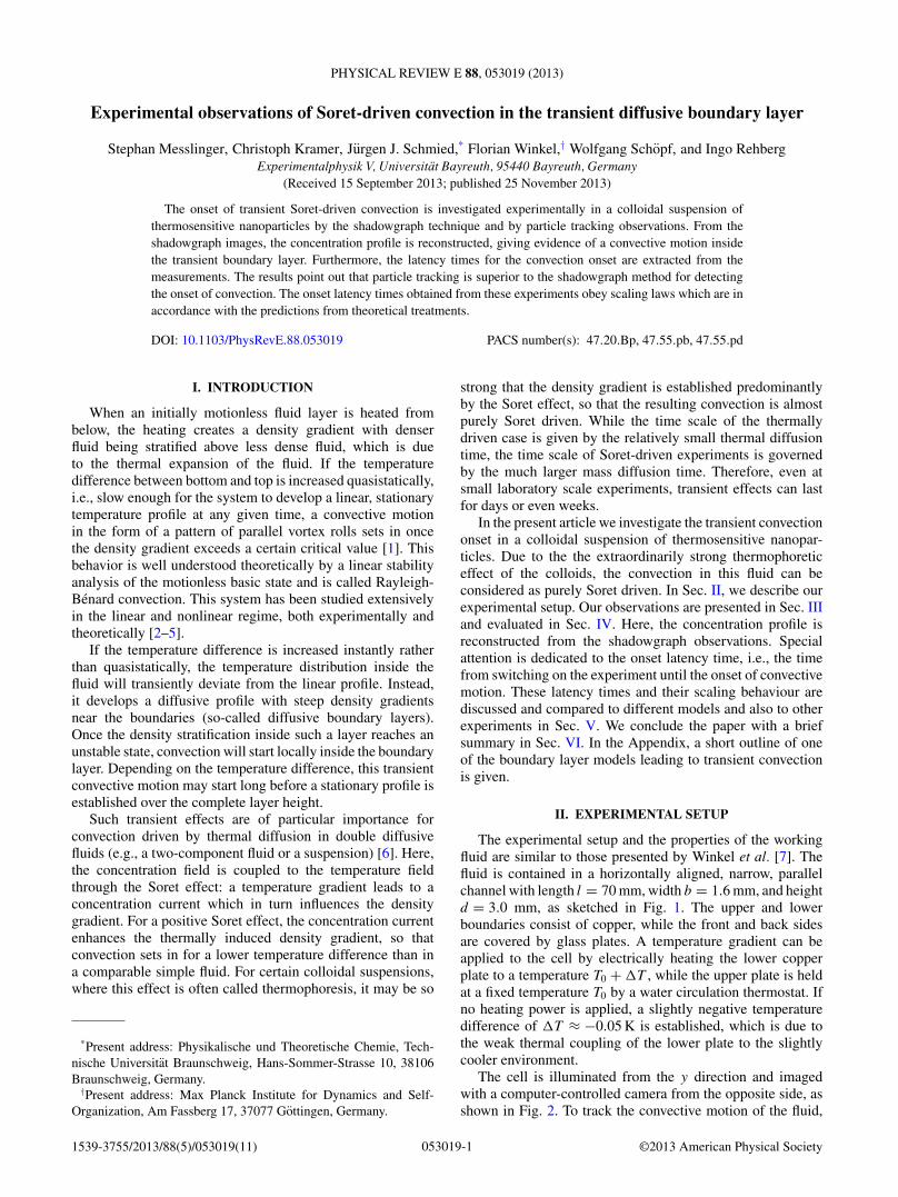
The experimental setup and the properties of the workingfluid are similar to those presented by Winkel et al. [7]. Thefluid is contained in a horizontally aligned, narrow, parallelchannel with length l = 70 mm, width b = 1.6 mm, and heightd = 3.0 mm, as sketched in Fig. 1. The upper and lowerboundaries consist of copper, while the front and back sidesare covered by glass plates. A temperature gradient can beapplied to the cell by electrically heating the lower copperplate to a temperature T0 + �T , while the upper plate is heldat a fixed temperature T0 by a water circulation thermostat. Ifno heating power is applied, a slightly negative temperaturedifference of �T ≈ −0.05 K is established, which is due tothe weak thermal coupling of the lower plate to the slightlycooler environment.

The cell is illuminated from the y direction and imagedwith a computer-controlled camera from the opposite side, asshown in Fig. 2. To track the convective motion of the fluid,

053019-11539-3755/2013/88(5)/053019(11) ©2013 American Physical Society

STEPHAN MESSLINGER et al. PHYSICAL REVIEW E 88, 053019 (2013)

d

b

l

Cu

glass

fluid

z

xy

dbl

= 3.0 mm= 1.6 mm= 70 mmT + T0 Δ

T0

g

FIG. 1. Schematic representation of the convection cell.

fluorescent polystyrene tracer particles1 with a diameter of2 μm and a density comparable to that of the fluid are added.The concentration of tracer particles has a number density ofapproximately 1900/mm3, corresponding to a mass fraction ofapproximately 8 ppm of polystyrene in water. Although withthis setup we can only measure the x-z position of the particles,a movement in the y direction can be detected qualitativelyfrom the change of the diffraction patterns produced bymovements perpendicular to the focus plane.

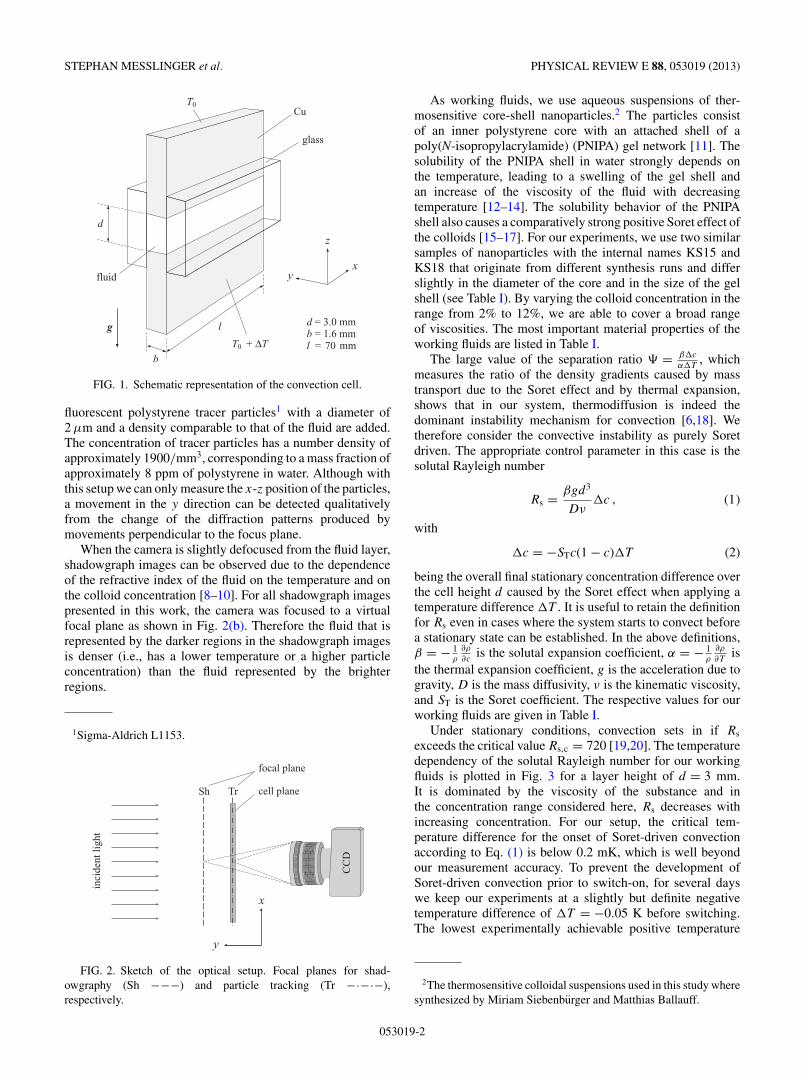
When the camera is slightly defocused from the fluid layer,shadowgraph images can be observed due to the dependenceof the refractive index of the fluid on the temperature and onthe colloid concentration [8–10]. For all shadowgraph imagespresented in this work, the camera was focused to a virtualfocal plane as shown in Fig. 2(b). Therefore the fluid that isrepresented by the darker regions in the shadowgraph imagesis denser (i.e., has a lower temperature or a higher particleconcentration) than the fluid represented by the brighterregions.

1Sigma-Aldrich L1153.

CC

D

focal plane

y

x

inci

dent

ligh

t

cell planeSh Tr

FIG. 2. Sketch of the optical setup. Focal planes for shad-owgraphy (Sh −−−) and particle tracking (Tr −·−·−),respectively.

As working fluids, we use aqueous suspensions of ther-mosensitive core-shell nanoparticles.2 The particles consistof an inner polystyrene core with an attached shell of apoly(N-isopropylacrylamide) (PNIPA) gel network [11]. Thesolubility of the PNIPA shell in water strongly depends onthe temperature, leading to a swelling of the gel shell andan increase of the viscosity of the fluid with decreasingtemperature [12–14]. The solubility behavior of the PNIPAshell also causes a comparatively strong positive Soret effect ofthe colloids [15–17]. For our experiments, we use two similarsamples of nanoparticles with the internal names KS15 andKS18 that originate from different synthesis runs and differslightly in the diameter of the core and in the size of the gelshell (see Table I). By varying the colloid concentration in therange from 2% to 12%, we are able to cover a broad rangeof viscosities. The most important material properties of theworking fluids are listed in Table I.

The large value of the separation ratio � = β�c

α�T, which

measures the ratio of the density gradients caused by masstransport due to the Soret effect and by thermal expansion,shows that in our system, thermodiffusion is indeed thedominant instability mechanism for convection [6,18]. Wetherefore consider the convective instability as purely Soretdriven. The appropriate control parameter in this case is thesolutal Rayleigh number

Rs = βgd3

Dν�c , (1)

with

�c = −STc(1 − c)�T (2)

being the overall final stationary concentration difference overthe cell height d caused by the Soret effect when applying atemperature difference �T . It is useful to retain the definitionfor Rs even in cases where the system starts to convect beforea stationary state can be established. In the above definitions,β = − 1

ρ

∂ρ

∂cis the solutal expansion coefficient, α = − 1

ρ

∂ρ

∂Tis

the thermal expansion coefficient, g is the acceleration due togravity, D is the mass diffusivity, ν is the kinematic viscosity,and ST is the Soret coefficient. The respective values for ourworking fluids are given in Table I.

Under stationary conditions, convection sets in if Rs

exceeds the critical value Rs,c = 720 [19,20]. The temperaturedependency of the solutal Rayleigh number for our workingfluids is plotted in Fig. 3 for a layer height of d = 3 mm.It is dominated by the viscosity of the substance and inthe concentration range considered here, Rs decreases withincreasing concentration. For our setup, the critical tem-perature difference for the onset of Soret-driven convectionaccording to Eq. (1) is below 0.2 mK, which is well beyondour measurement accuracy. To prevent the development ofSoret-driven convection prior to switch-on, for several dayswe keep our experiments at a slightly but definite negativetemperature difference of �T = −0.05 K before switching.The lowest experimentally achievable positive temperature

2The thermosensitive colloidal suspensions used in this study wheresynthesized by Miriam Siebenburger and Matthias Ballauff.

053019-2

EXPERIMENTAL OBSERVATIONS OF SORET-DRIVEN . . . PHYSICAL REVIEW E 88, 053019 (2013)

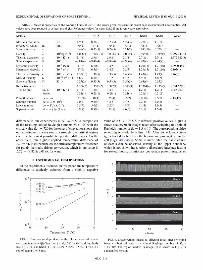
TABLE I. Material properties of the working fluids at 25 ◦C. The errors given represent the worst-case measurement uncertainties. Allvalues have been rounded to at least two digits. Reference values for water [21,22] are given where applicable.

Material KS18 KS15 KS18 KS18 KS18 KS18 Water

Mass concentration c (%) 11.9(1) 8.7(2) 7.20(5) 5.29(3) 2.28(1) 1.91(1) —Hydrodyn. radius Rh (nm) 70(1) 77(1) 70(1) 70(1) 70(1) 70(1) —Volume fraction 0.48(5) 0.32(5) 0.29(5) 0.21(2) 0.093(10) 0.077(10) —

Density ρ (103 kg m−3) 1.008(1) 1.0053(1) 1.0042(1) 1.0023(1) 0.9993(1) 0.9989(1) 0.997 047(1)Thermal expansion α (10−4 K−1) 3.1(1) 2.9(1) 2.9(1) 2.8(1) 2.7(1) 2.7(1) 2.572 922(3)Solutal expansion β (10−2) −9.84(4) −9.46(4) −9.89(4) −9.90(4) −9.93(4) −9.94(4) —

Dynamic viscosity η (10−3 Pa s) 17(6) 6.6(6) 3.4(5) 2.2(3) 1.29(15) 1.21(10) 0.8900(15)Kinematic viscosity ν (10−6 m2 s−1 17(6) 6.5(5) 3.4(5) 2.2(3) 1.29(15) 1.21(10) 0.893(1)

Thermal diffusivity κ (10−7 m2 s−1) 1.33(10) 1.36(5) 1.38(5) 1.40(5) 1.43(4) 1.43(4) 1.46(3)Mass diffusivity D (10−12 m2 s−1) 8.6(2) 6.8(4) 7.1(5) 6.7(5) 5.9(6) 5.8(7) —Soret coefficient ST (K−1) 0.27(2) 0.35(3) 0.54(3) 0.54(3) 0.63(6) 0.65(6) —

Refractive index n 1.356(2) 1.3507(2) 1.347(1) 1.343(1) 1.3364(4) 1.3356(4) 1.331 62(2)(632.8 nm) ∂n/∂T (10−4 K−1) −1.7(4) −1.3(1) −1.4(3) −1.3(2) −1.2(1) −1.2(1) −1.055 090

∂n/∂c 0.21(1) 0.23(1) 0.21(1) 0.21(1) 0.21(1) 0.21(1) —

Prandtl number Pr = ν/κ 127(50) 48(4) 25(4) 16(2) 9.0(10) 8.5(7) 6.13(12)Schmidt number Sc = ν/D (105) 2.0(7) 9.5(9) 4.8(8) 3.4(5) 2.2(3) 2.1(3) —Lewis number Le = D/κ (10−5) 6.5(5) 5.0(3) 5.2(4) 4.8(4) 4.1(4) 4.1(5) —Separation ratio � = − β

αSTc(1 − c) 8.9(7) 8.8(8) 12(8) 9.6(6) 5.2(5) 4.5(4) —

difference in our experiments is �T = 0.05. A comparisonof the resulting solutal Rayleigh numbers Rs > 105 with thecritical value Rs,c = 720 for the onset of convection shows thatour experiments always run in a strongly overcritical regimeeven for the lowest possible temperature differences. On theother hand, our highest applied temperature difference of�T ≈ 6 K is still well below the critical temperature differencefor purely thermally driven convection, which in our setup is�T w

c = (9.82 ± 0.01) K for water.

III. EXPERIMENTAL OBSERVATIONS

In the experiments discussed in this paper, the temperaturedifference is suddenly switched from a slightly negative

15 25 35106

107

108

Temperature (°C)T

1.91 %

11.9 %

5.29 %7.20 %

8.71 %

2.28 %

20 30

FIG. 3. Temperature dependence of the relevant material param-

eter combination − βgd3

DνSTc(1 − c) = Rs/�T for the working fluids

KS15 (8.71%) and KS18 (1.91%, 2.28%, 5.29%, 7.20%, 11.9%) in acell of height d = 3 mm.

value of �T ≈ −0.05 K to different positive values. Figure 4shows shadowgraph images taken after switching to a solutalRayleigh number of Rs = 1.3 × 108. The corresponding videorecording is available online [23]. After some latency timetlat, a front detaches from the bottom and propagates into thecell [Figs. 4(a)–4(c)]. Some minutes later, the same courseof events can be observed starting at the upper boundary,which is not shown here. After a disordered interlude lastingfor several hours, a stationary convection pattern establishes

x (mm)

24 min(a)

0

3

0 5 10 15 20

27 min(b)

0

3

30 min(c)

0

3

0

3 6 h(d)

z(m

m)

FIG. 4. Shadowgraph images at different times after switchingfrom a subcritical state to a solutal Rayleigh number of Rs =1.3 × 108. The region marked in image (c) is shown in Fig. 7 ina magnified version.

053019-3

STEPHAN MESSLINGER et al. PHYSICAL REVIEW E 88, 053019 (2013)

z

xy

(a)

(b)

(c)

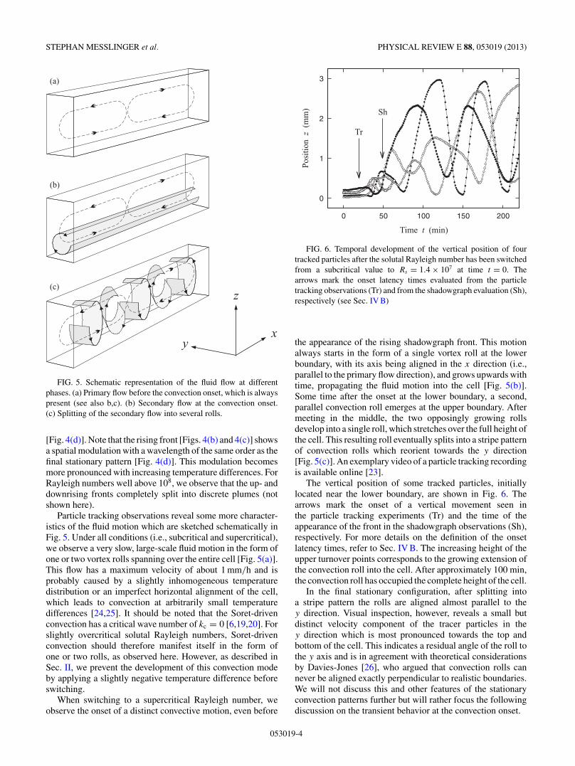
FIG. 5. Schematic representation of the fluid flow at differentphases. (a) Primary flow before the convection onset, which is alwayspresent (see also b,c). (b) Secondary flow at the convection onset.(c) Splitting of the secondary flow into several rolls.

[Fig. 4(d)]. Note that the rising front [Figs. 4(b) and 4(c)] showsa spatial modulation with a wavelength of the same order as thefinal stationary pattern [Fig. 4(d)]. This modulation becomesmore pronounced with increasing temperature differences. ForRayleigh numbers well above 108, we observe that the up- anddownrising fronts completely split into discrete plumes (notshown here).

Particle tracking observations reveal some more character-istics of the fluid motion which are sketched schematically inFig. 5. Under all conditions (i.e., subcritical and supercritical),we observe a very slow, large-scale fluid motion in the form ofone or two vortex rolls spanning over the entire cell [Fig. 5(a)].This flow has a maximum velocity of about 1 mm/h and isprobably caused by a slightly inhomogeneous temperaturedistribution or an imperfect horizontal alignment of the cell,which leads to convection at arbitrarily small temperaturedifferences [24,25]. It should be noted that the Soret-drivenconvection has a critical wave number of kc = 0 [6,19,20]. Forslightly overcritical solutal Rayleigh numbers, Soret-drivenconvection should therefore manifest itself in the form ofone or two rolls, as observed here. However, as described inSec. II, we prevent the development of this convection modeby applying a slightly negative temperature difference beforeswitching.

When switching to a supercritical Rayleigh number, weobserve the onset of a distinct convective motion, even before

0

1

2

3

0 50 100 150 200

Pos

itio

n(m

m)

z

Time (min)t

Sh

Tr

FIG. 6. Temporal development of the vertical position of fourtracked particles after the solutal Rayleigh number has been switchedfrom a subcritical value to Rs = 1.4 × 107 at time t = 0. Thearrows mark the onset latency times evaluated from the particletracking observations (Tr) and from the shadowgraph evaluation (Sh),respectively (see Sec. IV B)

the appearance of the rising shadowgraph front. This motionalways starts in the form of a single vortex roll at the lowerboundary, with its axis being aligned in the x direction (i.e.,parallel to the primary flow direction), and grows upwards withtime, propagating the fluid motion into the cell [Fig. 5(b)].Some time after the onset at the lower boundary, a second,parallel convection roll emerges at the upper boundary. Aftermeeting in the middle, the two opposingly growing rollsdevelop into a single roll, which stretches over the full height ofthe cell. This resulting roll eventually splits into a stripe patternof convection rolls which reorient towards the y direction[Fig. 5(c)]. An exemplary video of a particle tracking recordingis available online [23].

The vertical position of some tracked particles, initiallylocated near the lower boundary, are shown in Fig. 6. Thearrows mark the onset of a vertical movement seen inthe particle tracking experiments (Tr) and the time of theappearance of the front in the shadowgraph observations (Sh),respectively. For more details on the definition of the onsetlatency times, refer to Sec. IV B. The increasing height of theupper turnover points corresponds to the growing extension ofthe convection roll into the cell. After approximately 100 min,the convection roll has occupied the complete height of the cell.

In the final stationary configuration, after splitting intoa stripe pattern the rolls are aligned almost parallel to they direction. Visual inspection, however, reveals a small butdistinct velocity component of the tracer particles in they direction which is most pronounced towards the top andbottom of the cell. This indicates a residual angle of the roll tothe y axis and is in agreement with theoretical considerationsby Davies-Jones [26], who argued that convection rolls cannever be aligned exactly perpendicular to realistic boundaries.We will not discuss this and other features of the stationaryconvection patterns further but will rather focus the followingdiscussion on the transient behavior at the convection onset.

053019-4

EXPERIMENTAL OBSERVATIONS OF SORET-DRIVEN . . . PHYSICAL REVIEW E 88, 053019 (2013)

17.016.816.616.4

(mm)x

(a)

0

0.5

1

1.5

2

2.5

3

z(m

m)

-0.2 -0.1 0 0.1 0.2

(b)

-0.8 -0.6 -0.4 -0.2 0

Concentration

(arb. units)

(c)

Normalized Intensity

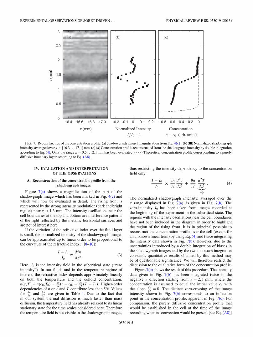
FIG. 7. Reconstruction of the concentration profile. (a) Shadowgraph image [magnification from Fig. 4(c)]. (b) (�) Normalized shadowgraphintensity, averaged over x ∈ [16.3 . . . 17.1] mm. (c) (•) Concentration profile reconstructed from the shadowgraph intensity by double integrationaccording to Eq. (4). Only the range z = 0.5 . . . 2.1 mm has been evaluated. (- - -) Theoretical concentration profile corresponding to a purelydiffusive boundary layer according to Eq. (A8).

IV. EVALUATION AND INTERPRETATIONOF THE OBSERVATIONS

A. Reconstruction of the concentration profile from theshadowgraph images

Figure 7(a) shows a magnification of the part of theshadowgraph image which has been marked in Fig. 4(c) andwhich will now be evaluated in detail. The rising front isrepresented by the strong intensity modulation (dark and brightregion) near z ≈ 1.3 mm. The intensity oscillations near thecell boundaries at the top and bottom are interference patternsof the light reflected by the metallic horizontal surfaces andare not of interest here.

If the variation of the refractive index over the fluid layeris small, the normalized intensity of the shadowgraph imagescan be approximated up to linear order to be proportional tothe curvature of the refractive index n [8–10]:

I − I0

I0∝ d2n

dz2. (3)

Here, I0 is the intensity field in the subcritical state (“zerointensity”). In our fluids and in the temperature regime ofinterest, the refractive index depends approximately linearlyon both the temperature and the colloid concentration:n(c,T ) − n(c0,T0) = ∂n

∂c(c − c0) + ∂n

∂T(T − T0). Higher-order

dependencies of n on c and T contribute less than 5%. Valuesfor ∂n

∂cand ∂n

∂Tare given in Table I. Due to the fact that

in our system thermal diffusion is much faster than massdiffusion, the temperature field has already relaxed to its linearstationary state for the time scales considered here. Thereforethe temperature field is not visible in the shadowgraph images,

thus restricting the intensity dependency to the concentrationfield only:

I − I0

I0∝ ∂n

∂c

d2c

dz2+ ∂n

∂T

d2T

dz2︸︷︷︸=0

. (4)

The normalized shadowgraph intensity, averaged over thex range displayed in Fig. 7(a), is given in Fig. 7(b). Thezero-intensity I0 has been taken from images recorded atthe beginning of the experiment in the subcritical state. Theregions with the intensity oscillations near the cell boundarieshave not been included in the diagram in order to highlightthe region of the rising front. It is in principal possible toreconstruct the concentration profile over the cell (except foran unknown linear term) by using Eq. (4) and twice integratingthe intensity data shown in Fig. 7(b). However, due to theuncertainties introduced by a double integration of biases inthe shadowgraph images and by the two unknown integrationconstants, quantitative results obtained by this method maybe of questionable significance. We will therefore restrict thediscussion to the qualitative form of the concentration profile.

Figure 7(c) shows the result of this procedure. The intensitydata given in Fig. 7(b) has been integrated twice in thenegative z direction starting from z = 2.1 mm, where theconcentration is assumed to equal the initial value c0 withthe slope dc

dz= 0. The distinct zero-crossing of the image

intensity shown in Fig. 7(b) corresponds to an inflectionpoint in the concentration profile, apparent in Fig. 7(c). Forcomparison, the purely diffusive concentration profile thatwould be established in the cell at the time of the imagerecording when no convection would be present [see Eq. (A8)]

053019-5

STEPHAN MESSLINGER et al. PHYSICAL REVIEW E 88, 053019 (2013)

0

Pos

itio

n z

(m

m)

Time (min)t

0

0.5

1

1.5

2

20 25 30 35 40

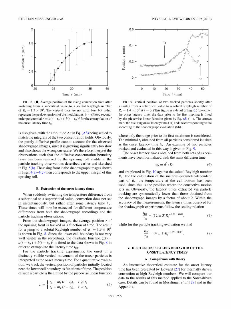
FIG. 8. (�) Average position of the rising convection front afterswitching from a subcritical value to a solutal Rayleigh numberof Rs = 1.3 × 108. The vertical bars are not error bars but ratherrepresent the peak extensions of the modulations. (- - -) Fitted second-order polynomial z = a(t − tlat) + b(t − tlat)2 for the extrapolation ofthe onset latency time tlat.

is also given, with the amplitude �c in Eq. (A8) being scaled tomatch the integrals of the two concentration fields. Obviously,the purely diffusive profile cannot account for the observedshadowgraph images, since it is growing significantly too slowand also shows the wrong curvature. We therefore interpret theobservations such that the diffusive concentration boundarylayer has been remixed by the uprising roll visible in theparticle tracking observations described earlier and sketchedin Fig. 5(b). The rising front in the shadowgraph images shownin Figs. 4(a)–4(c) then corresponds to the upper margin of thisuprising roll.

B. Extraction of the onset latency times

When suddenly switching the temperature difference froma subcritical to a supercritical value, convection does not setin instantaneously, but rather after some latency time tlat.These times will now be extracted for different temperaturedifferences from both the shadowgraph recordings and theparticle tracking observations.

From the shadowgraph images, the average position z ofthe uprising front is tracked as a function of time. The resultfor a jump to a solutal Rayleigh number of Rs = 1.3 × 108

is shown in Fig. 8. Since the lower cell boundary is not verywell visible in the recordings, the quadratic function z(t) =a(t − tlat) + b(t − tlat)2 is fitted to the data shown in Fig. 8 inorder to extrapolate the latency time tlat.

For the particle tracking experiments, the onset of adistinctly visible vertical movement of the tracer particles isinterpreted as the onset latency time. For a quantitative evalua-tion, we track the vertical position of particles initially locatednear the lower cell boundary as functions of time. The positionof such a particle is then fitted by the piecewise linear function

z ={

zc + mf (t − tc), t � tc

zc + mc (t − tc), t < tc,(5)

0

0.2

0.4

0.6

0 10 20 30 40 50

Pos

itio

n(m

m)

z

Time (min)t

Sh

Tr

FIG. 9. Vertical position of two tracked particles shortly aftera switch from a subcritical value to a solutal Rayleigh number ofRs = 1.4 × 107 at t = 0. (This figure is a detail of Fig. 6.) To extractthe onset latency time, the data prior to the first maxima is fittedby the piecewise linear function given by Eq. (5) (—). The arrowsmark the resulting onset latency time (Tr) and the corresponding valueaccording to the shadowgraph evaluation (Sh).

where only the range prior to the first maximum is considered.The minimal tc obtained from all particles considered is takenas the onset latency time tlat. An example of two particlestracked and evaluated in this way is given in Fig. 9.

The onset latency times obtained from both sets of experi-ments have been normalized with the mass diffusion time

τD = d2/D (6)

and are plotted in Fig. 10 against the solutal Rayleigh numberRs. For the calculation of the material-parameter-dependentpart of Rs, the temperature at the cell bottom has beenused, since this is the position where the convective motionsets in. Obviously, the latency times extracted via particletracking are systematically lower than those obtained fromthe shadowgraph images by a factor of about 2. Within theaccuracy of the measurements, the latency times observed forthe shadowgraph experiments follow the scaling relation

tlat

τD= (12 ± 3)R −0.51 ± 0.01

s , (7)

while for the particle tracking evaluation we find

tlat

τD= (4 ± 1)R −0.49 ± 0.03

s . (8)

V. DISCUSSION: SCALING BEHAVIOR OF THEONSET LATENCY TIMES

A. Comparison with theory

An instructive theoretical estimate for the onset latencytime has been presented by Howard [27] for thermally drivenconvection at high Rayleigh numbers. We will compare ourdata to the results of this method applied to the Soret-drivencase. Details can be found in Messlinger et al. [28] and in theAppendix.

053019-6

EXPERIMENTAL OBSERVATIONS OF SORET-DRIVEN . . . PHYSICAL REVIEW E 88, 053019 (2013)

5

10-3

2

5

10-2

106 107 108 109

Howard’s method

Integral methodKim

[31]

Solutal Rayleigh number

Ons

etla

tenc

yti

me

Particle tracking

12 %8.7 %5.3 %Eq. (8)

Shadowgraph

8.7 %7.2 %5.3 %2.3 %1.9 %Eq. (7)

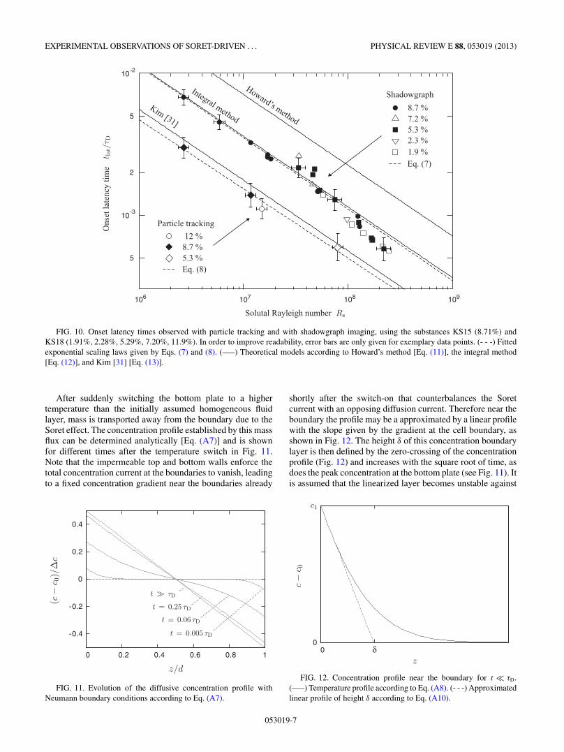
FIG. 10. Onset latency times observed with particle tracking and with shadowgraph imaging, using the substances KS15 (8.71%) andKS18 (1.91%, 2.28%, 5.29%, 7.20%, 11.9%). In order to improve readability, error bars are only given for exemplary data points. (- - -) Fittedexponential scaling laws given by Eqs. (7) and (8). (—–) Theoretical models according to Howard’s method [Eq. (11)], the integral method[Eq. (12)], and Kim [31] [Eq. (13)].

After suddenly switching the bottom plate to a highertemperature than the initially assumed homogeneous fluidlayer, mass is transported away from the boundary due to theSoret effect. The concentration profile established by this massflux can be determined analytically [Eq. (A7)] and is shownfor different times after the temperature switch in Fig. 11.Note that the impermeable top and bottom walls enforce thetotal concentration current at the boundaries to vanish, leadingto a fixed concentration gradient near the boundaries already

-0.4

-0.2

0

0.2

0.4

0 0.2 0.4 0.6 0.8 1

FIG. 11. Evolution of the diffusive concentration profile withNeumann boundary conditions according to Eq. (A7).

shortly after the switch-on that counterbalances the Soretcurrent with an opposing diffusion current. Therefore near theboundary the profile may be a approximated by a linear profilewith the slope given by the gradient at the cell boundary, asshown in Fig. 12. The height δ of this concentration boundarylayer is then defined by the zero-crossing of the concentrationprofile (Fig. 12) and increases with the square root of time, asdoes the peak concentration at the bottom plate (see Fig. 11). Itis assumed that the linearized layer becomes unstable against

00 δ

FIG. 12. Concentration profile near the boundary for t � τD.(—–) Temperature profile according to Eq. (A8). (- - -) Approximatedlinear profile of height δ according to Eq. (A10).

053019-7

STEPHAN MESSLINGER et al. PHYSICAL REVIEW E 88, 053019 (2013)

convection once the “local” solutal Rayleigh number

rs = βgδ3

Dν�c , (9)

corresponding to Eq. (1) but calculated over the boundary layerheight δ only, exceeds the threshold criterium for a stationaryprofile, i.e., for rs > Rs,c. This happens at a critical boundarylayer height δ∗,

δ∗

d=

(Rs

Rs,c

)−1/4

≈ 5.34 R−1/4s , (10)

which is reached after the latency time tlat,

tlat

τD= π

4

(Rs

Rs,c

)−1/2

≈ 22.4 R−1/2s , (11)

after the switch-on. In this formulation, the explicit depen-dencies on the material parameters of the fluid are hidden inthe global Rayleigh number Rs, which is also a convenientmacroscopic control parameter for the experiment. For theexplicit prefactors given on the right-hand sides of Eqs. (10)and (11), a critical Rayleigh number of Rs,c = 816.74 hasbeen assumed [19,20]. This corresponds to a mechanicallyrigid lower and stress-free upper boundary, in order to accountfor the possibility of lateral fluid motion at the upper side of theconcentration boundary layer, which is typically well insidethe fluid layer and not close to the rigid upper wall. Since tlat

only depends on the square root of Rs,c, however, the actualchoice of the value for Rs,c does not change the magnitude oftlat significantly.

Alternatively, as proposed by Shliomis and Souhar [29],the height of the concentration boundary layer may be definedby requiring the integral over the concentration profile to beconserved. This leads to a reduced prefactor in the scalingrelation for the onset latency time:

tlat

τD= 1√

2π

(Rs

Rs,c

)−1/2

≈ 11.4 R−1/2s . (12)

Note that for both methods, the stability criteria appliedhere are valid only for horizontally infinitely extended fluidlayers, while for narrow channels, other scaling relations apply[28]. Although the experiments discussed here are run in anarrow channel rather than in a bulk fluid layer, the criticallayer heights at the convection onset according to Eq. (10)are significantly smaller than the cell thickness: δ∗ < 0.1 d <

0.2 b for the solutal Rayleigh numbers of Rs > 106 appliedhere. Therefore, at the convection onset, the cell boundariesare still far away compared to the concentration layer height,so that the scaling relation for the bulk geometry is appropriate.

It is well known that the stability analyses of nonlineartemperature profiles yield significantly lower critical Rayleighnumbers than those of the corresponding linear profiles [30]. Astability analysis of the full nonlinear transient profile evolvingin a Soret-driven experiment has been presented by Kim [31],who reports a scaling relation for the onset time of

tlat

τD≈ 5.58 R−1/2

s . (13)

The theoretical scaling relations [Eqs. (11)–(13)] derived bythe different methods are shown together with the experimental

data in Fig. 10. The exponential scaling behavior of theonset latency times measured in our experiments is in goodagreement with these models. The absolute values extractedfrom the shadowgraph recordings coincide very well with theprefactor in Eq. (12), derived by the integral method, while thevalues obtained from the particle tracking recordings agreewith the result of Eq. (13) by Kim [31].

The discrepancy of the onset latency times predicted bythe theoretical treatment and observed experimentally by theshadowgraph method is well known. It is often attributedto the fact that after the real latency time, some additionalgrowth period has to pass until the convection flow issufficiently strong to be experimentally detectable with theshadowgraph method [31,32]. This argument is supported byour observation, where the convection onset detected withparticle tracking coincides well with the order of magnitudepredicted by the theory, while the shadowgraph evaluationyields systematically larger values.

B. Comparison with other experiments

Cerbino et al. [33] have investigated Soret-driven convec-tion of a colloidal suspension with a large negative separationratio in a bulk experiment heated from above at high solutalRayleigh numbers of Rs = 106 . . . 109. They report the onsetlatency time to follow the relation tlat/τD = 25.3 R−0.52±0.03

s .Nielsen and Sabersky [34] observed the onset of thermally

driven convection of silicone oils in a bulk geometry heatedfrom below with a constant heat flux over the bottom boundary.Due to this boundary condition, their system can be consideredmathematically equivalent to the Soret-driven case, if thesolutal Rayleigh number is replaced by the normal Rayleighnumber R. From their data we extract a scaling for the onsetlatency times of tlat/τD = 20 R−0.5.

In both studies, the convection was observed with theshadowgraph technique, looking from above. Both scalingrelations show the same exponential behavior as in ourexperiments, however, with slightly larger prefactors. Keepingin mind the different geometries and observation techniquesof the experiments, the agreement of the onset latency timesis amazingly good.

VI. SUMMARY AND CONCLUSION

We have investigated the onset of transient, Soret-drivenconvection experimentally by particle tracking and shad-owgraph methods. The onset latency times evaluated fromboth methods obey the theoretically predicted exponentialscaling laws. However, particle tracking observations revealthat the convective fluid motion sets in significantly earlierthan detectable by the shadowgraph method. The onset latencytime extracted from particle tracking observations is mostaccurately described by the theoretical analysis of Kim [31].Although our experiments were conducted in a narrow cell,in the range of large solutal Rayleigh numbers investigatedhere, it is plausible that the convection onset in a bulkfluid layer shows a similar behavior. The respective particletracking experiments in bulk geometries have yet to bedone.

053019-8

EXPERIMENTAL OBSERVATIONS OF SORET-DRIVEN . . . PHYSICAL REVIEW E 88, 053019 (2013)

ACKNOWLEDGMENTS

We thank Roberto Cerbino, Alberto Vailati, Gora Conley,and Simon Wongsuwarn for stimulating discussions, andAndreas Koniger and Werner Kohler for their helpful adviceconcerning the measurement of refractive indices and Soretcoefficients. Special thanks goes to Miriam Siebenburger andMatthias Ballauff for providing the PNIPA core-shell colloids.Financial support of the Deutsche Forschungsgemeinschaft(DFG) through the Forschergruppe FOR608, Convection inSuspensions project is gratefully acknowledged.

APPENDIX: LATENCY TIME SCALING FOR THECONVECTION ONSET IN A TRANSIENT DIFFUSIVE

BOUNDARY LAYER ESTABLISHED BYTHE SORET EFFECT

We consider a fluid layer of height d, infinitely extendedin the horizontal directions, so that in the motionless state, thesystem may be treated as one-dimensional (i.e., z directiononly). The fluid consists of two components, with the mixingratio being described by the mass concentration c = m1/(m1 +m2), which is assumed to be initially homogeneously dis-tributed:

c(z,t = 0) = c0 . (A1)

Apart from the ordinary mass diffusion, the fluid componentsare subject to an additional mass transport due to the Soreteffect, resulting in a total concentration current

j = −D[∂zc + STc(1 − c)∂zT ], (A2)

with ST being the Soret coefficient and D the mass diffusioncoefficient [6,35]. The horizontal walls at z = 0,d are assumedto be impermeable, so that the concentration current is forcedto vanish at the boundaries:

j |z=0 = j |z=d = 0 . (A3)

For the following discussion, we will assume all concentrationchanges to be sufficiently small compared to the initiallyuniform profile, so that the factor STc(1 − c) ≈ STc0(1 − c0)remains approximately constant.

When applying a temperature difference �T to the cellboundaries, mass will be transported along the temperaturegradient, until for large times t τD = d2/D, the Soret-driven transport is just balanced by the diffusive reverse flow.In the stationary case, a total concentration difference of

�c = −STc0(1 − c0)�T (A4)

will have been achieved between the cell boundaries.Since the thermal diffusion is typically much faster than

the mass diffusion (τκ = d2/κ � τD due to κ D), wemay assume that on the time scale of the Soret effect, thereis always a fully developed stationary temperature profile∂zT = −�T/d = const., independent of the applied thermalboundary conditions. The continuity equation inferred fromEq. (A2) is then reduced to a homogeneous diffusion equation

∂tc = −∂zj = D ∂2z c, (A5)

with Neumann boundary conditions enforced by the imperme-able walls [Eq. (A3)]

∂zc |z=0 = ∂zc |z=d = STc0(1 − c0)�T

d= −�c

d(A6)

at the top and bottom boundaries [36].To simplify the expressions, in the following discussion

we will treat �c as the experimentally controllable parameter,which always denotes the total concentration difference that,according to Eq. (A4), would have built up in the equilibriumstate, even if the system becomes unstable against convectionmuch earlier, as discussed below.

The analytical solution to the Neumann problem stated byEqs. (A5) and (A6) together with the initial condition (A1) canbe expressed by a Fourier expansion:

c(z,t) = c0 + �c

[1

2− z

d−

∞∑n=1

8 cos(qnz)

(2n − 1)2π2e−Dq2

n t

]

with qn = (2n − 1)π

d. (A7)

The temporal development is shown in Fig. 11. For t τD, thelinear stationary profile according to Eq. (A4) will be achieved.Note that due to the Neumann boundary conditions (A6), theconcentration gradient ∂zc at the boundaries is forced to itsfinal stationary value already at the very beginning. Also notethat the concentration profile in Fig. 11 is normalized to �c.For a positive �T (i.e., heated from below) and a positiveST, �c is negative and the resulting concentration profile ismonotonically rising.

For t � τD, we can treat the system as two independentwalls with infinite distance. In this limit, Eq. (A7) canbe approximated by the analytical solutions of switch-onprocesses at two semi-infinite half-spaces [37]. The profilenear the lower boundary is then given by

c(z,t) = c0 + �c

[2

d

√Dt

πexp

(−z2

4Dt

)− z

derfc

(z

2√

Dt

)]

= c0 + �c

[2

π1/2

√t

τDexp

(− (z/d)2

4 t/τD

)

− z

derfc

(z/d

2√

t/τD

)], (A8)

∂zc(z,t) = �c

derfc

(z

2√

Dt

)= �c

derfc

(z/d

2√

t/τD

).

(A9)

The corresponding profile near the upper wall is obtained bysubstituting z → d − z in Eqs. (A8) and (A9).

Following the method introduced by Howard [27], weapproximate the concentration field near the boundary by alayer with a linear concentration profile

clin(z,t) − c0 = c1

(1 − z

δ

), (A10)

with

c1 = c(z = 0,t) = �c

d2

√Dt

π= 2�c

π1/2

√t

τD(A11)

053019-9

STEPHAN MESSLINGER et al. PHYSICAL REVIEW E 88, 053019 (2013)

being the concentration at the boundary (see Fig. 12). Theslope of the profile is given by the gradient at the boundary,∂zc(z = 0,t) = −�c/d, which yields a layer height δ of

δ(t) = − c1

∂c/∂z

∣∣∣∣z=0

= 2

√Dt

π= 2d

π1/2

√t

τD, (A12)

defined by the zero-crossing of the linear profile. We nowconsider a “local” solutal Rayleigh number rs calculated onlyover the linearized boundary layer of thickness δ:

rs = βg

Dνδ3c1 = βg

Dνd3�c

24

π2

(t

τD

)2

. (A13)

Dividing the local Rayleigh number by the correspondingexpression for the global Rayleigh number [Eq. (1)] yields

rs

Rs= 24

π2

(t

τD

)2

. (A14)

Again following Howard [27], we will assume that theboundary layer profile becomes unstable against convectiononce its local Rayleigh number rs exceeds the critical valueRs,c, corresponding to a stationary density profile. The latencytime tlat from switching on the temperature difference untilrs(tlat) = Rs,c is

tlat

τD= π

4︸︷︷︸≈0.79

(Rs

Rs,c

)−1/2

. (A15)

The “critical” height of the boundary layer at this instant oftime is δ∗ = δ(tlat):

δ∗

d=

(Rs

Rs,c

)−1/4

. (A16)

An alternative definition for the layer height, presented byShliomis and Souhar [29], is to require the integral over theconcentration profile to be conserved:

∫ δ

01 − z

δdz =

∫ ∞

0erfc

(z

2√

κt

)dz , (A17)

resulting in a layer height

δ(t) =√

πDt = dπ1/2

√t

τD, (A18)

and slightly different prefactors for the onset latency time andcritical layer height:

tlat

τD= 1√

2π︸ ︷︷ ︸≈0.40

(Rs

Rs,c

)−1/2

, (A19)

δ∗

d=

(π

2

)1/4

︸ ︷︷ ︸≈1.1

(Rs

Rs,c

)−1/4

. (A20)

[1] S. Chandrasekhar, Hydrodynamic and Hydromagnetic Stability(Oxford University Press, Oxford, UK, 1961).

[2] F. H. Busse and J. A. Whitehead, J. Fluid Mech. 47, 305 (1971).[3] F. H. Busse, Rep. Prog. Phys. 41, 1929 (1978).[4] M. C. Cross and P. C. Hohenberg, Rev. Mod. Phys. 65, 851

(1993).[5] E. Bodenschatz, W. Pesch, and G. Ahlers, Annu. Rev. Fluid

Mech. 32, 709 (2000).[6] J. K. Platten and J. C. Legros, Convection in Liquids (Springer,

New York, 1984).[7] F. Winkel, S. Messlinger, W. Schopf, I. Rehberg,

M. Siebenburger, and M. Ballauff, New J. Phys. 12, 053003(2010).

[8] S. Rasenat, G. Hartung, B. L. Winkler, and I. Rehberg, Exp.Fluids 7, 412 (1989).

[9] W. Schopf, J. C. Patterson, and A. M. H. Brooker, Exp. Fluids21, 331 (1996).

[10] W. Merzkirch, Flow Visualization (Academic Press, New York,1987).

[11] M. Ballauff and Y. Lu, Polymer 48, 1815 (2007).[12] M. Siebenburger, M. Fuchs, and M. Ballauff, Soft Matter 8,

4014 (2012).[13] H. Senff, W. Richtering, C. Norhausen, A. Weiss, and

M. Ballauff, Langmuir 15, 102 (1999).[14] J. Crassous, A. Wittemann, M. Siebenburger, M. Schrinner,

M. Drechsler, and M. Ballauff, Colloid Polym. Sci. 286, 805(2008).

[15] R. Kita and S. Wiegand, Macromolecules 38, 4554 (2005).

[16] S. Wongsuwarn, R. C. D. Vigolo, A. M. Howe, A. Vailati,R. Piazza, and P. Cicuta, Soft Matter 8, 5857 (2012).

[17] A. Koniger, N. Plack, W. Kohler, M. Siebenburger, andM. Ballauff, Soft Matter 9, 1418 (2013).

[18] B. Huke, H. Pleiner, and M. Lucke, Phys. Rev. E 75, 036203(2007).

[19] P. Colinet, J. C. Legros, and M. G. Velarde, Nonlinear Dynamicsof Surface-Tension-Driven Instabilities (Wiley-VCH, New York,2001).

[20] D. A. Nield and A. Bejan, Convection in Porous Media, 3rd ed.(Springer, New York, 2006).

[21] IAPWS, Release on the refractive index of ordinary watersubstance as a function of wavelength, temperature and pressure,Available at http://www.iapws.org (1997).

[22] IAPWS, Supplementary release on properties of liquid water at0.1 MPa, Available at http://www.iapws.org (2008).

[23] See Supplemental Material at http://link.aps.org/supplemental/10.1103/PhysRevE.88.053019 for video recordings of the tran-sient convection onset.

[24] K. E. Daniels, B. B. Plapp, and E. Bodenschatz, Phys. Rev. Lett.84, 5320 (2000).

[25] J. E. Hart, J. Fluid Mech. 47, 547 (1971).[26] R. P. Davies-Jones, J. Fluid Mech. 44, 695 (1970).[27] L. N. Howard, in Proceedings of the 11th International Congress

of Applied Mechanics, Munich (Germany) 1964, edited byH. Gortler (Springer, New York, 1966), pp. 1109–1115.

[28] S. Messlinger, W. Schopf, and I. Rehberg, Int. J. Heat MassTransfer 62, 336 (2013).

053019-10

EXPERIMENTAL OBSERVATIONS OF SORET-DRIVEN . . . PHYSICAL REVIEW E 88, 053019 (2013)

[29] M. I. Shliomis and M. Souhar, Europhys. Lett. 49, 55 (2000).[30] D. A. Nield, J. Fluid. Mech. 71, 441 (1975).[31] M. C. Kim, Eur. Phys. J. E 34, 27 (2011).[32] C. K. Choi, J. H. Moon, T. J. Chung, M. C. Kim, K. H. Ahn,

S.-T. Hwang, and E. J. Davis, Int. J. Heat Mass Transfer 55,1030 (2012).

[33] R. Cerbino, S. Mazzoni, A. Vailati, and M. Giglio, Phys. Rev.Lett. 94, 064501 (2005).

[34] R. C. Nielsen and R. H. Sabersky, Int. J. Heat Mass Transfer 16,2407 (1973).

[35] S. Wiegand, J. Phys.: Condens. Matter 16, R357(2004).

[36] D. Hurle and E. Jakeman, J. Fluid Mech. 47, 667(1971).

[37] J. Crank, The Mathematics of Diffusion, 2nd ed. (OxfordUniversity Press, Oxford, UK, 1986).

053019-11