Embed Size (px)
Citation preview

VOT 78123
EXPERIMENTAL INVESTIGATION ON THE BEHAVIOUR OF
THERMAL EFFLUENT IN FREE SURFACE FLOW
(KAJIAN EKSPERIMEN TERHADAP KELAKUNAN EFLUEN
TERMA DI DALAM ALIRAN SALURAN TERBUKA)
ZULKIFLEE BIN IBRAHIM
DR. NOOR BAHARIM BIN HASHIM
ASSOC. PROF. ABD. AZIZ BIN ABDUL LATIFF
HERNI BINTI HALIM
NURUL HANA BINTI MOKHTAR KAMAL
NURYAZMEEN FARHAN BINTI HARON
RESEARCH VOTE NO:
78123
Jabatan Hidraul & Hidrologi
Fakulti Kejuruteraan Awam
Universiti Teknologi Malaysia
2008

ii
ACKNOWLEDGEMENT
First and foremost, we would like to express our gratitude towards the Ministry of
Higher Education (MOHE), Malaysia and Research Management Centre (RMC),
Universiti Teknologi Malaysia (UTM) for their financial support for this research.
Our sincere appreciation to Dr. Suhaimi Abu Bakar (Department of Structure &
Material, Faculty of Civil Engineering, UTM) for introducing the DPIV method and Dr.
Yeak Su Hoe (Department of Mathematics, Faculty of Science, UTM) for the application
of Maple software in this study.
We also would like to share our gratitude towards all staffs of Hydraulics and
Hydrology Laboratory, Faculty of Civil Engineering, Universiti Teknologi Malaysia for
their help and support during the experiments and work.
Last but not least, our greatest appreciation is extended to all the students who
have involved in this study. This research will not be completed without their continuous
hard work.

iii
THE BEHAVIOUR OF SUBMERGED CROSS-FLOW THERMAL
EFFLUENT DISCHARGE IN FREE SURFACE FLOW
(Keywords: Thermal effluent, multi-port diffuser, cross-flow, dispersion, near-field)
Thermal discharges such as from power station or industries polluting inland water bodies (rivers) causing degradation of water quality. The density of heated fluid is less than cold fluid and the positive buoyancy will force the heated fluid to disperse and spread at the ambient surface when it is discharged into the water bodies. Good understanding on thermal effluent behaviour in waterbodies leads good discharge management which can minimise the impact of thermal effluent pollution. An experimental study is conducted in the laboratory to investigate the mechanism of heat transport in free surface flow for ambient and thermal effluent flow rates. A multi-port diffuser pipe is placed at the channel bed in cross-flow direction to the ambient flow. Thermal effluent flow rates, Qe used in the experiment are 0.05 liter/s and 0.133 liter/s. Meanwhile, two ambient flow rates, Qa are fixed at 20 liter/s and 10 liter/s. The research focuses on thermal mixing process in near-field region. Among the parameters studied are effluent temperature, hydraulics characteristics of ambient flow (flow rate and velocity) and the characteristics of open channel including length, depth, and width. The dispersion profiles of thermal effluent are observed at various locations along the channel through the plotted isothermal lines. Meanwhile, the results of excess temperature (∆T/Te) show that it decreases with the increasing of dispersion rate, KT as the thermal effluent moves downstream of the channel. The changes of ambient temperature, ∆T are studied through the plotted graphs. The results show that mixing process occurs in near-field and far-field regions. The temperature differences in near-field region are higher than far-field region because the area experienced high thermal effluent temperature, Te. Meanwhile, temperature differences in far-field region are low due to the effect of mixing between thermal effluent and ambient flow.
Key researchers :
Zulkiflee Ibrahim Dr. Noor Baharim Hashim
Prof. Madya Abd. Aziz Abdul Latiff Herni Halim
Nurul Hana Mokhtar Kamal Nuryazmeen Farhan Haron
E-mail : [email protected] Tel. No. : 07-5531764 Vote No. : 78123

iv
KAJIAN EKSPERIMEN TERHADAP KELAKUNAN EFLUEN
TERMA DI DALAM ALIRAN TERBUKA
(Kata kunci: Efluen terma, paip peresap pelbagai liang, aliran menegak, medan dekat)
Pelepasan haba daripada stesyen janakuasa atau industri mencemarkan sungai dan menyebabkan pengurangan kualiti air. Ketumpatan air panas adalah rendah berbanding air sejuk dan daya keapungan positif akan menyebabkan air panas tersebar ke permukaan ambien apabila dilepaskan ke dalam sungai. Pemahaman yang baik dalam proses penyerakan effluen berhaba dalam sungai membawa kepada pengurusan pelepasan yang baik yang mana dapat mengurangkan kesan pencemaran haba. Kajian makmal dijalankan untuk mengkaji mekanisma pergerakan haba di dalam saluran terbuka pada kadar alir ambien dan effluen berhaba yang berbeza. Paip peresap pelbagai liang diletakkan di dasar saluran secara berserenjang dengan arah aliran ambien dalam sebuah saluran terbuka dengan kadar alir effluen berhaba, Qe yang digunakan dalam eksperimen adalah tetap iaitu 0.05 liter/s dan 0.133 liter/s. Selain itu,dalam kajian ini, dua kadar alir ambien, Qa yang ditetapkan iaitu 20.0 liter/s dan 10.0 liter/s digunakan. Proses percampuran effluen berhaba di dalam saluran tertumpu di kawasan medan dekat. Antara parameter yang terlibat dalam kajian adalah suhu effluen, ciri-ciri hidraulik aliran ambien (kadar alir dan halaju), dan ciri-ciri saluran terbuka termasuk panjang, dalam dan lebar. Corak serakan effluen berhaba pada setiap stesen cerapan di sepanjang saluran diperhatikan melalui plotan garisan isotermal. Sementara itu, excess temperature, ∆T/Te menurun dengan peningkatan kadar serakan, KT apabila semakin jauh pergerakan effluen terma di dalam saluran. Perubahan suhu ambien, ∆T dikaji melalui plotan graf. Keputusan yang diperolehi menunjukkan proses percampuran dalam kawasan medan dekat dan medan jauh. Perubahan suhu pada medan dekat adalah sangat tinggi kerana mengalami percampuran dengan effluen berhaba yang bersuhu tinggi, Te. Manakala, perubahan suhu pada medan jauh adalah rendah kerana suhu effluen berhaba telah menurun akibat kesan proses percampuran dengan aliran ambien.
Penyelidik:
Zulkiflee Ibrahim Dr. Noor Baharim Hashim
Prof. Madya Abd. Aziz Abdul Latiff Herni Halim
Nurul Hana Mokhtar Kamal Nuryazmeen Farhan Haron
E-mail : [email protected] No.Tel. : 07-5531764 No.Vot : 78123

v
TABLE OF CONTENTS
TITLE PAGE
ACKNOWLEDGEMENT ii
ABSTRACT iii
ABSTRAK iv
TABLE OF CONTENTS v
LIST OF TABLES ix
LIST OF FIGURES x
LIST OF PHOTOS xiv
LIST OF SYMBOLS xv
LIST OF APPENDICES xvi
CHAPTER 1 INTRODUCTION 1
1.1 Introduction 1
1.2 Statement of Problem 3
1.3 Objectives of the Research 3
1.4 Scope of Study 4

vi
CHAPTER 2 LITERATURE REVIEW 6
2.1 Introduction 6
2.2 Terminologies 10
2.3 Characteristics of Thermal Effluent Discharge System 11
2.3.1 Ambient Parameters 12
2.3.2 Thermal Effluent Parameters 12
2.4 Heat Transport 13
2.5 Mixing Processes 13
2.5.1 Near-Field 15
2.5.2 Far-Field 18
2.6 Velocity of Ambient 15
2.7 Co-Flow Mixing 22
2.8 Jet Mixing 23
2.9 Excess Temperature and Dispersion Rate 25
2.10 Digital Particle Image Velocimetry (DPIV) Method 26
2.11 Previous Researches 27
2.11.1 Study by Kim Dae Geun and Il Won Seo (1999) 28
2.11.2 Study by Zimmermann and Geldner (1978) 29
2.11.3 Study by Davidson et al. (2001) 30
2.11.4 Study by Davies et al. (1994) 32
CHAPTER 3 METHODOLOGY 33
3.1 Introduction 33
3.2 Experimental Setup 34
3.3 Dimensional Analysis 37
3.4 Measurement of Ambient Flow Rate 39
3.5 Measurement of Ambient Velocity 40

vii
3.6 Measurement of Thermal Effluent Flow Rate 40
3.7 Measurement of Water Temperature 41
3.8 Experimental Procedure 44
3.9 Data Analysis 44
3.9.1 Effluent Dispersion Rate 45
3.9.2 Excess Temperature and Dispersion Rate 45
CHAPTER 4 FINDINGS AND DISCUSSION 46
4.1 Introduction 46
4.2 Ambient Flow Characteristics 47
4.3 Velocity Profile 49
4.4 Digital Particle Image Velocimetry (DPIV) Method 51
4.5 Effluent Dispersion Patterns 53
4.5.1 Dispersion Pattern in Near-Field (x/d=30) 53
4.5.2 Dispersion Pattern in Far-Field (x/d=110)
4.6 Excess Temperature, ∆T/Te 61
4.6.1 Effect of Different Qe on Excess Temperature
for a Constant Qa of 20 liter/s 62
4.6.2 Effect of Different Qe on Excess Temperature
for a Constant Qa of 10 liter/s 66
4.6.3 Effect of Different Qa on Excess Temperature
for a Constant Qe of 0.133 liter/s 69
4.6.4 Effect of Different Qa on Excess Temperature
for A Constant Qe of 0.05 liter/s 72
4.7 Dispersion Rate, KT 75
4.7.1 Effect of Different Qe on Dispersion Rate for
a Constant Qa of 20 liter/s 76
4.7.2 Effect of Different Qe on Dispersion Rate for

viii
a Constant Qa of 10 liter/s 79
4.7.3 Effect of Different Qa on Dispersion Rate for
a Constant Qe at 0.133 liter/s 83
4.7.4 Effect of Different Qa on Dispersion Rate for
a Constant Qe at 0.05 liter/s 85
4.8 Ambient Temperature Differences, ∆T with
Dimensionless Time, t* 88
CHAPTER 5 CONCLUSION AND RECOMMENDATIONS
5.1 Conclusion 91
5.2 Recommendations 92
REFERENCES 94
APPENDIX A 97
APPENDIX B 105

ix
LIST OF TABLES
TABLE NO.
TITLE PAGE
2.1 Thermal effluent sources with capacity
and percentage
7
3.1 Temperature observation stations along
x- axis
42
3.2 Temperature observation stations along
y- axis
42
3.3 Temperature observation stations along
z-axis for Qa of 10 liter/s
43
3.4 Temperature observation stations along
z- axis for Qa of 20 liter/s
36
4.1 Ratio of effluent and ambient flow rates
(Qe/Qa) used in the study
47
4.2 Ratio of effluent and ambient flow rates
(Qe/Qa) used in the study.
48

x
LIST OF FIGURES
FIGURE NO.
TITLE PAGE
2.1
2.2
Location of Tanjung Bin Power Plant along
the western banks of the Sungai Pulai
Near-field and far-field regions within
effluent discharges in a river
8
14
2.3 Ambient currents gradually deflect the
buoyant jet into the current direction
16
2.4 A two – dimensional buoyant jet plane 17
2.5 Vertical buoyant jet in cross-flow 20
2.6 A vortex pair in cross-flow 21
2.7 Ring vortices near the nozzles 21
2.8 Co-flow mixing of effluent in water body 22
2.9 Example of velocity vectors of buoyant jet
using DPIV method
27
2.10 Internal boundary condition for submerge
multi-port diffuser
28
3.1 The setup of experimental work 36
3.2 The developed rating curve for the study 39
4.1 Normalised ambient velocity 49
4.2a Velocity vectors using DPIV method for
ambient flow of Qa of 20 liter/s
52
4.2b Velocity vectors using DPIV method for
ambient flow of Qa of 10 liter/s
52
4.3a Cross-sectional ∆T (in 0C) at x/d = 30 for
Qa = 20.0 liter/s and Qe = 0.05 liter/s
54

xi
4.3b Cross-sectional ∆T (in 0C) at x/d = 30 for
Qa = 20.0 liter/s and Qe = 0.133 liter/s
55
4.4a Cross-sectional ∆T (in 0C) at x/d = 30 for
Qa = 10.0 liter/s and Qe = 0.05 liter/s
56
4.4b Cross-sectional ∆T (in 0C) at x/d = 30 for
Qa = 10.0 liter/s and Qe = 0.133 liter/s
57
4.5a
4.5b
4.6a
4.6b
4.7
Cross-sectional ∆T (in 0C) at x/d = 110 for
Qa = 20.0 liter/s and Qe = 0.05 liter/s
Cross-sectional ∆T (in 0C) at x/d = 110 for
Qa = 20.0 liter/s for Qe of 0.133 liter/s
Cross-sectional ∆T (in 0C) at x/d = 110 for
Qa = 10.0 liter/s and Qe = 0.05 liter/s
Cross-sectional ∆T (in 0C) at x/d = 110 for
Qa = 10.0 liter/s and Qe = 0.133 liter/s.
Longitudinal excess temperature profile,
∆T/Te for Qa of 20.0 liter/s at lower layer of
flow for different Qe.
58
58
60
60
64
4.8
4.9
4.10
4.11
Longitudinal excess temperature profile,
∆T/Te for Qa of 20.0 liter/s at middle layer
of flow for different Qe.
Longitudinal excess temperature profile,
∆T/Te for Qa of 20.0 liter/s at upper layer of
flow for different Qe.
Longitudinal excess temperature profile,
∆T/Te for Qa of 10.0 liter/s at lower layer of
flow for different Qe.
Longitudinal excess temperature profile,
∆T/Te for Qa of 10.0 liter/s at middle layer
of flow for different Qe.
65
65
68
68

xii
4.12
4.13
4.14
4.15
4.16
4.17
4.18
4.19
4.20
4.21
Longitudinal excess temperature profile,
∆T/Te for Qa of 10.0 liter/s at upper layer of
flow for different Qe.
Longitudinal excess temperature profile,
∆T/Te for Qe of 0.133 liter/s at lower layer
of flow for different Qa.
Longitudinal excess temperature profile,
∆T/Te for Qe of 0.133 liter/s at middle layer
of flow for different Qa
Longitudinal excess temperature profile,
∆T/Te for Qe of 0.133 liter/s at upper layer
of flow for different Qa.
Longitudinal excess temperature profile,
∆T/Te for Qe of 0.05 liter/s at lower layer of
flow for different Qa.
Longitudinal excess temperature profile,
∆T/Te for Qe of 0.05 liter/s at middle layer
of flow for different Qa.
Longitudinal excess temperature profile,
∆T/Te for Qe of 0.05 liter/s at upper layer of
flow for different Qa.
Longitudinal dispersion rate profile, KT for
Qa of 20.0 liter/s at lower layer of flow for
different Qe.
Longitudinal dispersion rate profile, KT for
Qa of 20.0 liter/s at middle layer of flow for
different Qe.
Longitudinal dispersion rate profile, KT for
Qa of 20.0 liter/s at upper layer of flow for
different Qe.
69
71
71
72
74
74
75
78
78
79

xiii
4.22
4.23
4.24
4.25
4.26
4.27
4.28
4.29
4.30
4.31
Longitudinal dispersion rate profile, KT for
Qa of 10.0 liter/s at lower layer of flow for
different Qe.
Longitudinal dispersion rate profile, KT for
Qa of 10.0 liter/s at middle layer of flow for
different Qe.
Longitudinal dispersion rate profile, KT for
Qa of 10.0 liter/s at upper layer of flow for
different Qe.
Longitudinal dispersion rate profile, KT for
Qe of 0.133 liter/s at lower layer of flow for
different Qa.
Longitudinal dispersion rate profile, KT for
Qe of 0.133 liter/s at middle layer of flow
for different Qa.
Longitudinal dispersion rate profile, KT for
Qe of 0.133 liter/s at upper layer of flow for
different Qa.
Longitudinal dispersion rate profile, KT for
Qe of 0.05 liter/s at lower layer of flow for
different Qa.
Longitudinal dispersion rate profile, KT for
Qe of 0.05 liter/s at middle layer of flow for
different Qa.
Longitudinal dispersion rate profile, KT for
Qe of 0.05 liter/s at upper layer of flow for
different Qa.
Temporal changes on temperature
difference for Qa of 20 liter/s at x/d of 30
and x/d of 110
81
82
82
84
84
85
86
87
87
89

xiv
4.32 Temporal changes on temperature
difference for Qa of 10 liter/s at x/d of 30
and x/d of 110
90
LIST OF PHOTOS
PHOTO NO.
TITLE PAGE
3.1
3.2
3.3
3.4
3.5
3.6
4.1
4.2
7.0 m long, 0.3 m wide and 0.3 m deep
glass flume
YSI 30 Salinity, Conductivity, and
Temperature (SCT)
PVC pipe with 5 holes and 12 mm diameter
each multi-port diffuser
A submersible portable pump, a PVC pipe
and overhead thermal effluent tank
2 axis electromagnetic Valeport current
meter model 802
Locations of digital thermometer at
different depths in the flume
Trajectory of thermal effluent discharge in
the channel (Qe= 0.05 liter/s, Qa=10 liter/s)
Trajectory of thermal effluent discharge in
the channel (Qe=0.133 liter/s, Qa=10 liter/s)
34
35
35
36
40
41
50
50

xv
LIST OF SYMBOLS
ν = kinematic viscosity
cρ∆ = density difference between ambient and effluent flow
aρ = ambient density
g = gravity celerity
v = velocity of ambient flow
R = hydraulics radius of ambient flow
T∆ = temperature difference
eT = effluent temperature
aT = ambient temperature
eQ = effluent flow rate
aQ = ambient flow rate
KT = dispersion rate
V = water volume in tank
Ad = area of of multi-port diffuser
Re = Reynolds Number
FD = Densimetric Froude Number
Fr = Froude Number
te = time taken to discharge thermal effluent
t = time taken to observe temperature in channel
t* = dimensionless time
u = ambient velocity
x = horizontal distance from discharge point
y = transverse distance from channel wall
z = vertical distance from bed of channel
d = diameter of port
H = flow depth

xvi
LIST OF APPENDICES
APPENDIX NO.
TITLE PAGE
A
B
Dimensional Analysis
Data
97
105

CHAPTER 1
INTRODUCTION
1.1 Introduction
In this new modern era, technologies keep developing each single day to fulfil
human needs. With each new technology introduced, our natural environment will be
more polluted as the volume from effluents created increases. Pollution can be defined
as the existence or addition of some organics or inorganic substances into the
environment that can damage part of the entire ecosystem. One of the most severe
polluted media is the hydrosphere or usually known as water.
The water serves as one of the environmental continuum; along with soil and
air which are dynamically interactive. In other words, with a change in one of these
elements, it will generate the changes in the other elements. Despite dealt as a whole,
these three elements always managed separately without considering the consequences
for the other elements. The characteristic of water that flows and carries substances as
it flows makes it one of the main pollutant transporters.

2
Hydrothermal pollution is one of water pollution forms. Hydrothermal
pollution can be defined as a change of temperature in water bodies caused by human
influences. Water used by power plants as coolant (i.e a fluid which flows through a
device in order to prevent its overheating, transferring the heat produced by the device
to other devices that utilize or dissipate it) is one of the main source of thermal
pollution in rivers.
Excessive heat transferred into the water will typically decrease the
concentration of dissolved oxygen in the water. This will result in the harming of
aquatic life such as amphibians and copepods, increased in metabolic rate of aquatic
life; resulting in the aquatic life consuming more food in shorter time compared to
normal environment. As the environment changes, the population of aquatic life may
decrease due to lack of food source, migration and in-migration of aquatic life to a
more suitable environment. The food chain may be disrupted as competition for fewer
resources took place.
From air temperature measurements constructed from land stations, a 0.5 °C
warming occurred during the past 100 years in the United States (Schneider, 1989 in
Singh and Hager, 1996). This might be the effects of human activities on the heat
balance of the earth by direct release of stored energy at a rate faster than natural
process, release of greenhouse gases and particulates and alteration of earth’s albedo
(Singh and Hager, 1996).
In preventing the rapid increasing of the earth temperature in the future, the
effluents from the industrial and technologies need to be controlled. This will lessen
the thermal pollution from occurring which will be affecting the stability of the
ecosystem.

3
1.2 Statement of Problem
The number of power plants constructed lately has rise as the demand for
power consumption has increased causing the higher volume of heated water
discharged into rivers. With the increasing volume of discharged heated water, the
ecosystem of the river may become unstable. Thermal pollution seems to affect the
aquatic life immediately after the discharge. Evaporative water losses, dissolved
oxygen production and consumption, primary biological productivity, toxicity of
pollutants, fish growth and reproduction are examples of processes affected by water
temperature changes. The most significant effect of temperature increase in rivers is
the dissolved oxygen level. As the temperature increased, the level of dissolved
oxygen decreased especially in the lower layers. In addition, because of the direct
thermal shock, most aquatic life can be killed with the abrupt temperature change that
goes beyond the tolerance limit of their metabolic systems.
Therefore, a study on the impact of thermal effluent released into a river
system should be carried out. The behaviour of thermal effluent discharged in ambient
flow is presented based on formula and calculation.
1.3 Objectives of the Research
This study describes an analysis of mixing of thermal effluent discharged from
multiport diffuser to ambient flow. The objectives of the study are:
(i) to investigate the mechanism of heat transport in channel flow,

4
(ii) to establish the relationships among parameter including ambient flow
conditions and heated flow properties, and
(iii) to investigate the impact of thermal discharges in inland water bodies.
1.4 Scope of Study
The scopes of this research comprise of two components: literature review and
laboratory experiments. The rationale of literature review is to expand information and
identify theories related to the study. Besides that, literature review is also carried out to
judge against the existing theories and the studies that have been carried out earlier.
According to literature review, several ideas and techniques to implement laboratory
study are gained besides identifying parameters involved based on previous studies. The
other important purpose of literature review is to identify the problems that may arise in
data collection during the laboratory experiments.
Before conducting a research, other than giving the main idea of the research,
literature review would help to determine the methods and techniques to be used in
data collection. Parameters to be observed through the experiments also can be
attained by reading literature review based on previous researches and theories. All of
the information for the literature review are obtained from books, journals,
encyclopedias, and from searched webs through the internet.
The laboratory experiment consists of the gathering of data by conducting series
of experiments on the heat transport in open channel. Independent parameters such as
effluent temperature and ambient discharge are adjusted to observe the relationship

5
between the parameters. In addition, Digital Particle Image Velocimetry (DPIV) method
is used to investigate mixing processes related to a buoyant jet phenomenon.

CHAPTER 2
LITERATURE REVIEW
2.1 Introduction
The pollution of rivers which occurred due to the operation of the factories and
power plants are getting worse if the discharges of the coolant from the plants into the
rivers are not controlled. Obviously, the simplest method of disposing the heated waste
water is to discharge them directly into the receiving water and allowed the natural
forces to bring the water back to an equilibrium temperature. Thermal effluent discharge
is released into the rivers using jet discharge system. The process of transporting
effluent in open channel depends on the density of the effluent. Thermal effluent
possesses lower density compared to ambient flow. Table 2.1 shows the thermal effluent
sources which uses water as coolant based from the research done by Rensselaer
Polytechnic Institute, New York. From Table 2.1, electric power generates the highest
percentage of thermal effluent discharge with 81.2%.

7
Table 2.1: Thermal effluent sources with capacity and percentage
(http://www.rpi.edu/dept)
Sources Cooling Water (Billions of m3) Cooling Water (in %)
Electric Power 153.7 81.2
Primary Metals 12.8 6.76
Chemical and Allied
Products 11.8 6.24
Others 10.9 5.80
Totals 189.2 100
An example of thermal effluent discharge through electric power plant is in
Tanjung Bin Power plant. Tanjung Bin has been designated as the industrial centre for
development of petrochemical and maritime industry under the Pontian District Plan
2002 to 2015 (Perunding Utama, 2003). This project of 2100 MW coal-fired power
plant is priority in order to meet the country projected growth in electric demand. The
project which has been identified by the Economic Planning Unit (EPU) of the Prime
Minister’s Department and Tenaga Nasional Berhad (TNB) has commercially
operational by the end of August 2006.
Tanjung Bin power plant is located at the southwestern tip of Peninsular
Malaysia along the western banks of the Sungai Pulai estuary. It also situated directly
opposite to the existing Port of Tanjung Pelepas (PTP) and its southern frontage is the
Straits of Johor as shown in Figure 2.1. The power plant with a nominal capacity of
2100 MW comprised of 3 turbine units of 700 MW capacity each. A once-through
cooling water system is employed, with the intake located in the Sungai Pulai and the
heated water discharged into the Straits of Johor to the southeast of the site.

8
Project Site
Figure 2.1: Location of Tanjung Bin Power Plant along the western banks of
the Sungai Pulai (Perunding Utama Sdn. Bhd., 2003)
The power plant uses Sungai Pulai as the source of water for plant cooling
processes. The water intake is located at the river mouth of Sungai Pulai. The warm
water discharged from the plant will affect thermal regime of Sungai Pulai. The thermal
pollution seems to only affect the communities immediately adjacent to the discharge.
Thermal discharge is most noted in the tropical areas, where faunal organisms are near
their maximum temperature tolerance.
In the worst-case scenario (during Mean Water Level after low water), a
possibility of 8 oC in temperature rise when all the 3 turbine units are operating at full
load. This will be only for a few hours in a day i.e during the morning and the evening
peak period in electricity consumption. During other times, the expected load will be
less than 90%, which resulted in a rise of less than 7 oC in condensers.

9
For the case of Tanjung Bin power plant, the site is surrounded by mangrove
vegetation. Although mangrove vegetation is generally very tolerant to thermal
pollution, the production rate has adversely affected producing fewer new seedlings
(Perunding Utama, 2003). In case of Tanjung Bin power plant the heated water
discharge produced an increase in water temperature to about 34 oC along the Sungai
Pulai and to a distance of 400 m from the outfall. According to Perunding Utama
(2003), temperature up to 40 oC does not visibly damage mangroves in short-term
effects. Moreover both species composition and biomass of mangrove root communities
are not affected adversely in temperature below 34 oC. However, the number of species
dropped abruptly between 34 oC and 35 oC. Above this temperature the number inversely
related to the water temperature.
For marine organisms, temperature of the water plays an important role in
organic reproduction, growth, maturity and longevity. The effects of temperature are
different for all organisms. An increase of 2.4 oC above the ambient level occurs during
the commencement of the plant. However, the ecological impact from the thermal
discharge is significantly only at the outfall itself with the temperature at the outfall
between 40 oC to 41 oC. The high temperature plume is limited to the immediate area of
the outfall (possibly not more than 50 m) and the temperature will fall rapidly with
mixing of the water.

10
2.2 Terminologies
The definitions of some of the physical transport process and terminologies that
would be significant in the research of heat transfer in open channel are:
i) Heat Transfer: A phenomenon of energy transfer which tended to
establish thermal equilibrium. The energy would be
moving from a region of higher temperature to the region
with lower temperature. The energy in transit is termed
heat.
ii) Thermal Pollution: A temperature change in natural water bodies caused by
human influence with adverse environmental effects in
aquatic system. A declination of the water bodies qualities
in physical, chemical and biological aspects as the water
bodies are polluted by the effluents of human activities
such as the industrial effluents.
iii) Dispersion: A phenomenon of particles or cloud of contaminants
scattering process by the combined effects of shear and
transverse diffusion.
iv) Buoyancy: Can be defined as the gravitational body force that acted
on a fluid of non-uniform density. Buoyancy produced as
the effluent is of lighter density being discharged into the
receiving water body of greater density. A temperature

11
variation can also resulted in the non-uniformity in fluid as
the fluid with higher temperature had lighter density. So,
it tended to float in the fluid with lower temperature with
higher density. The buoyancy is created by burning or by
heat conduction and radiation to the fluid. According to
Singh and Hager (1996) the flux buoyancy force, Fo, due
to the heat source is:
Fo = pc
Hg γ , (2.1)
where γ = the volume coefficient of thermal
expansion (percentage of volumetric
change per degree of temperature change)
H = the heat flux (energy per unit time)
Cp = specific heat at constant pressure (change
in energy per unit mass of fluid and per
degree of temperature change)
g = gravity acceleration
2.3 Characteristics of Thermal Effluent Discharge System
The hydrodynamic mixing process of any heated waste water discharge is
governed by the interaction of ambient parameters in the receiving water body and by
the thermal effluent parameters. Two main parameters for the mixing process that must
be observed are the ambient conditions and the discharge conditions.

12
2.3.1 Ambient Parameters
Parameters in open channel represent hydraulics characteristic of ambient flow.
According to Zimmerman and Geldner (1978) the parameters are open channel depth
(y0), open channel width (B0), flow velocity (vo), ambient water temperature (T0), bed
channel friction (ks), formation of river bed, course of the main flow and flow direction.
These parameters define type of flow in open channel either in laminar, transitional or
turbulent condition.
2.3.2 Thermal Effluent Parameters
The parameters of thermal effluent discharge in ambient flow are jet diameter
(d), flow velocity (ue), effluent temperature (Te), thermal effluent density ( eρ ), angle
between effluent outwards direction and ambient flow (α ).
All of the listed parameters are used in the calculation of the hydrodynamic
mixing process. Different types of outlet may illustrate different types of mixing
characteristics. For a single port discharge, the port diameter, the elevation above the
bottom and its orientation provided the geometric features. Meanwhile for multi-port
diffuser installations of the individual ports along the diffuser line, the orientation of the
diffuser line, and construction details represented additional geometric features.
The buoyancy flux represented the effects of the relative density difference
between the effluent discharge and ambient conditions in combination with the

13
gravitational acceleration. It is a measure of the tendency for the effluent flow to rise
(positive buoyancy) or to fall (negative buoyancy) in the water column.
2.4 Heat Transport
Heat transport occurs during the existence of a temperature difference in a
medium. Consequently, heat transport is defined as energy transfer due to temperature
difference. The three basic modes of heat transport are conduction, convection and
radiation (Stefan and Hondzo, 1996). Conduction arises by collision between
molecules. Due to this process, conduction is sometimes called the “invisible” heat
transport. Furthermore, convection is the heat transport in the presence of a moving
fluid. Besides, radiation is heat transport that occurs by electromagnetic waves. All
surface of finite temperature emit energy in the form of electromagnetic waves.
Water temperature levels and dynamics have a significant effect on aquatic
ecosystems. Evaporative water losses, dissolved oxygen production and consumption,
primary biological productivity, toxicity of pollutants, fish growth and reproduction are
examples of processes affected by water temperature changes. For all of these causes,
water temperature is considered as a key parameter of aquatic systems.
2.5 Mixing Processes
The mixing behaviour of thermal effluent discharge is governed by relationship
between ambient conditions (geometric and dynamic characteristics) and discharge

14
characteristics (geometric and flux). For multi-port diffuser setting up, the orientations
of the diffuser line and construction details are geometric features (Jirka et. al, 1996).
The fluctuation characteristics are given by the effluent discharge flow rate, momentum
fluctuation and buoyancy fluctuation.
A mixing process of an effluent continuously discharging into water body can be
separated in two regions. In the near-field region, the initial jet characteristics of
momentum flux, buoyancy flux, and outfall geometry influence the jet path and mixing.
As the turbulent plume travels further away from the source, conditions existing in the
ambient environment will control path. This region is known as far-field. Figure 2.2
illustrates near-field and far-field regions within effluent discharges in a river.
Figure 2.2: Near-field and far-field regions within effluent discharges in a river
(Stefan and Hondzo, 1996)

15
2.5.1 Near-Field
Near–field is a region of the receiving water where the initial jet characteristics
of momentum flux, buoyancy flux and outfall geometry influence the jet trajectory and
mixing of the effluent discharge. Three types of near-field processes are submerged
buoyant jet mixing, boundary relations and surface buoyant jet mixing.
For submerged buoyant jet mixing, the concept is that where both fluid
momentum and pollutants are gradually diffused into the ambient field. The effluent
flow from a submerged discharge port provides a velocity discontinuity between the
discharged fluid and the ambient fluid. this condition produces shear force. The
shearing flow breaks down rapidly into a turbulent movement. Any concentration of the
discharge flow is diluted by ambient water through turbulent movement.
The near-field is usually highly three-dimensional and turbulent, with high
dissipation of kinetic and potential energy of the discharged in the ambient fluid (Singh
and Hager, 1996). The basic equations which describe the incompressible multi-
dimensional fluid flow in the near-field written in index notation are the continuity,
momentum and heat conservation equations. The equations are as follow:
Continuity equation:
0=∂∂
i
i
xu (2.2)
Momentum equation:
)(''1aiji
j
i
jirj
ij
i TTguuxu
xxp
xu
utu
−−⎟⎟⎠
⎞⎜⎜⎝
⎛−
∂∂
∂∂
+∂∂
−=∂∂
+∂∂
βνρ
(2.3)

16
Heat Conservation equation:
⎟⎟⎠
⎞⎜⎜⎝
⎛−
∂∂
∂∂
=∂∂
+∂∂ '' Tu
xTK
xxTu
tT
ii
mii
i (2.4)
where ui = instantaneous velocity component in the xi direction (m/s)
Km = molecular thermal diffusivity
T = instantaneous temperature (˚C)
xi = wise stream direction (m)
Ambient currents and density stratification further affected the buoyant jet
mixing. The buoyant jets are gradually deflected by the ambient currents into the current
direction as shown in Figure 2.3 and thus induce additional mixing. The vertical
acceleration within the buoyant jet is counteracted by the ambient density stratification
eventually leading to trapping of flow at a certain level.
Figure 2.3: Ambient currents gradually deflect the buoyant jet into the current
direction (Jirka, et al., 1996)

17
In case of multi-port diffuser, the individual round buoyant jets behave
independently until they interact, or merge, with each other at a certain distance from the
efflux ports. At a certain distance from the efflux ports, the individual round buoyant
jets will merge, producing two dimensional buoyant jet planes as shown in Figure 2.4.
Such plane buoyant jets resulting from a multi-port diffuser discharge in deep water can
be further affected by ambient currents and density stratification.
Figure 2.4: A two–dimensional buoyant jet plane
Another process of near field is boundary interaction processes. Ambient water
bodies always have vertical boundaries. These include the water surface and the bottom,
but in addition, internal boundaries may exist at pycnoclines. Pycnoclines are layers of
rapid density change. Depending on the dynamic and geometric characteristics of the
discharge flow, a variety of interaction phenomena can occur at such boundaries,
particularly where flow trapping may occur.

18
2.5.2 Far-Field
Far-field is a region of the receiving water where the mixing processes are
characterized by the longitudinal advection of the mixed effluent by the ambient current
velocity. There are two processes at far–field. They are buoyant spreading processes
and passive ambient diffusion processes.
Buoyant spreading processes are defined as the horizontally transverse spreading
of the mixed effluent flow while it is being advected downstream by the ambient current.
Such spreading processes arise due to the buoyant forces caused by the density
difference of the mixed flow relative to the ambient density. They can be effective
transport mechanisms that can quickly spread a mixed effluent laterally over large
distances in the transverse direction, particularly in cases of strong ambient stratification.
In general, the passive diffusion flow grows in width and in thickness until it
interacts. The strength of the ambient diffusion mechanism depends on a number of
factors relating mainly to the geometry of the ambient shear flow and the amount of
ambient stratification.
2.6 Cross-flow Mixing
The cross-flow mixing or also known as vertical diffusion by Singh and Hager
(1996) in unstratified flow is usually estimated to be the same as the eddy viscosity;
which is obtained from the logarithmic velocity distribution and the linear distribution of

19
shear stress from channel bed to water surface. According to Fisher et al. (1979) this
method leads to:
ez = κK u* z (1- z/h) (2.5)
where κK is von Karman coefficient, u* is shear velocity, h is flow depth, and z is vertical
coordinate measured upward from the bed.
Equation 2.5 gives a parabolic distribution of ez and the “Reynolds analogy”
which states it is used in the development of concentration distributions for suspended
sediment which has been verified by Jobson and Sayre (1970) in Singh and Hager
(1996) by means of an experimental research of the vertical mixing of dye in a flume.
Averaging over the depth and κ = 0.4 gives:
*067.0 duez = (2.6)
where d is depth of boundary layer.
The characteristics of spreading and entrainment change significantly as jets and
plumes are deflected by a cross flow. Figure 2.5 shows vertical buoyant jet deflected by
cross flow. The analysis for the effects of the cross flow is often carried out by
considering the limitating cases of near-field and far-field separately. Wright (1977) in
Singh and Hager (1996) has classified the flow into four limitating cases:
(i) mdnf (momentum-dominated near-field)
(ii) bdnf (buoyancy-dominated near-field)
(iii) mdff (momentum-dominated far-field)
(iv) bdff (buoyancy-dominated far-field)

20
From the experimental data obtained, the entrainment process in the near-field
(mdnf and bdnf) is rather unaffected by the cross flow and is essentially the equivalent
as the jets and plumes. While at the far-field process (mdff and bdff) are closely related
to the vortex pair and is examined using a line impulse model. As in Figure 2.6, a vortex
pair is formed as the jets bends over towards the direction of cross flow. Figure 2.7
shows ring vortices near the nozzles in close look.
Figure 2.5: Vertical buoyant jet in cross-flow

21
Figure 2.6: A vortex pair in cross-flow
Figure 2.7: Ring vortices near the nozzles

22
2.7 Co-flow Mixing
Co-flow mixing is the condition where effluent is flow parallel water body flow.
Figure 2.8 shows co-flow mixing of effluent in water bodies. Also known as transverse
dispersion, co-flow takes place in rivers due to two categories of mechanism, namely
turbulence and intertwining of time-averaged streamlines, with turbulent mixing
between the streamlines.
Figure 2.8: Co-flow mixing of effluent in water body
The conditions that may create turbulence in rivers are bed shear and separation
at bed irregularities, flow circulation in pools of pool-and-riffle streams. Other than that,
flow separation at the inside of sharp bends or at the ends of groins, jetties, or other bank
protection also causes turbulence in rivers. In addition, flow confinement structures and
apparently by transverse shear associated with the transverse distribution of longitudinal
velocity also cause turbulence in rivers.
Streamlines intertwine occurs because of continual splitting and convergence of
streamlines in braided rivers, flow around bed irregularities in rivers with irregular cross
sections and secondary flow (e.g. helical flow in bends). Tracer test is conducted as it is

23
the most reliable method to obtain transverse dispersion coefficients (ky) for a river. In
conditions that a tracer test is not applicable, there are some general but very limited
results which can be used as guidance for the expected value of ky. Generalized values
for ky are normally given as non dimensional values for αy which is defined as
with H as average depth.
*/ Huk y
Previous researchers observed that, cross-flow mixing is better than co-flow
mixing. According to Afidah Murni et.al. (2004) and Ruzanna (2005), cross-flow
discharge produces higher dispersion rate compared to co-flow discharge.
2.8 Jet Mixing
In many researches of jet mixing, several factors are taken into consideration in
identifying jet process in mixing. Jet and plumes are defined as turbulent shear flows
driven by sources of momentum and buoyancy respectively. The mixing and dispersion
of the contaminants with the environment depend on the momentum and buoyancy flux
of the discharge, along with the velocity distribution and density stratification of the
receiving environment. Jet mixing is related directly to the inertia of the turbulent
eddies. The buoyant force in the plume produces the inertia which leads to mixing.
Meanwhile, in co–flow jet mixing, inertia force manipulate the mixing process
compared to buoyancy. Furthermore, immediate momentum is manipulated by buoyancy
and influence the formation of mixing zone in the flow.

24
The Froude number is the ratio of mean velocity to the celerity of the gravity
waves.
gLVFr = (2.7)
where, V = mean velocity (m/s)
g = acceleration of gravity (m/s2)
L = characteristic length ( or can be hydraulic depth, H in open channel) (m)
with Fr < 1 (subcritical flow)
Fr = 1 (critical flow)
Fr > 1 (supercritical flow)
In cross-flow discharge, buoyancy force reduces effluent dispersion rate in
vertical direction. Buoyancy effects is stated by Densimetric Froude number as shown in
equation 2.8 (Martin and McCutcheon, 1999):
FD =
a
c
gH
u
ρρ0∆
(2.8)
where , ∆ρο = difference of effluent density and ambient density
ρa = ambient density, kg/m3
uc = turbulent velocity at water surface parallel to the jet, m/s
H = vertical depth of jet, m
g = gravitational acceleration, m/s2
Densimetric Froude number, FD represents type of flow in jet mixing. FD equals
to 1 (FD = 1) shows that the flow in jet mixing is critical while FD less than 1 (FD < 1)

25
indicates that the flow is subcritical flow. FD more than 1 (FD > 1) denote that the type
of flow in jet mixing is supercritical flow (Martin and McCutcheon, 1999).
The Reynolds number represents the effect of viscosity relative to inertia which
is given as:
v
uL=Re (2.9)
where, u = flow velocity, m/s
L = Characteristic length (also can be considered as hydraulic radius, R for
open channel), m
υ = kinematic viscosity, m2/s
Turbulent flow has Re greater than 12,500 while Reynolds number for
transitional flow is between 500 and 12,500. Laminar flow has Re less than 500 (Chow,
1959).
2.9 Excess Temperature and Dispersion Rate
Excess temperature, ∆T/Te, is a normalisation of the temperature difference, ∆T,
in the water flow after the thermal effluent is being discharged. The equation for ∆T/Te
is :
∆T/Te = e
ax
TTT −
(2.10)

26
where Ta is ambient temperature (0C), Te is effluent temperature (0C), Tx is observed
temperature (0C) at distance x along the channel (Kuang and Lee, 2001).
Effluent dispersion rate, KT , can be defined as the cooling and dilution rate of the
thermal effluent discharged in the water flow. It is important in determining the
efficiency of a pipe diffuser system. Dispersion rate always inversely proportion to the
excess temperature. A small changes of temperatures gives higher dispersion rates.
Ambient flow velocity and distance from multiport diffuser influence dispersion rate in
open channel. from KT can be calculated using equation 2.11 (Pinheiro et al., 1997):
KT = ax
ae
TTTT
−− (2.11)
where Ta is ambient temperature (0C), Te is effluent temperature (0C), Tx is observed
temperature at distance x along the channel (0C).
2.10 Digital Particle Image Velocimetry (DPIV) Method
In recent years, the measuring techniques of Digital Particle Image Velocimetry
(DPIV) are broadly used to investigate mixing processes related to buoyant jets
phenomenon (Law and Wang, 1991). DPIV requires the projection of a laser sheet onto
the flow field at successive time intervals and the subsequent capturing of the images
detailing the position of seeding particles that reflect the laser light. Analysis of the
difference in positions of the particles reveals the Langragian velocity distribution of the
flow field.

27
The present setup improves on the accuracy of the measurements by adopting
fully digital approaches. The DPIV setup can measure at sub-pixel accuracy (typically
0.1 pixels). Through cross- correlation of two successive images in MATLAB software
using correlation of URAPIV file, the velocity vectors are readily determined with
DPIV. Figure 2.9 shows example of velocity vectors of buoyant jet using DPIV method.
Figure 2.9 : Example of velocity vectors of buoyant jet using DPIV method.
2.11 Previous Researches
Previous researches on thermal effluent discharge in open channel flow have
been carried out by several researches all over the world. Kim and Il (1999),
Zimmermann and Geldner (1978), Davidson et al., (2001), Davies et al., (1994) are
some of the researchers that actively involved in thermal effluent discharge studies.

28
2.11.1 Study by Kim Dae Geun and Il Won Seo (1999)
Kim Dae Geun and Il Won Seo have carried out an experimental study on
mixing of thermal effluent discharged from multi–port diffuser using three–dimensional
grid–based numerical model. For this study, the internal boundary is treated as a line
patch. Discharge flowrate, QN, from a cell of numerical slot diffuser can be determined
using equation 2.12.
QN = n.Iq.b.L.u(x) (2.12)
where n is number of ports included in a cell of numerical slot diffuser, Iq is shape
constants, b is effective width of single jet, L is port spacing and u(x) is jet centerline
velocity.
Figure 2.10: Internal boundary condition for submerge multiport diffuser.
Discharge excess temperature, ∆TN from a cell of numerical slot diffuser can be
determined by using equation 2.13.

29
∆TN = o
N
QQ ∆To (2.13)
where Qo is discharge flow rate from ports in a cell of numerical slot diffuser, ∆To is
discharge excess temperature from multi-port diffuser.
The research is concluded that pattern of thermal plume simulated by the
numerical model are agreeable with the observed thermal plume. Furthermore, excess
temperature is decreasing as ambient water depth is increasing. The result confirms the
previous study in which dilution of Tee shape diffuser varies sensitively with ambient
water depth. The simulation by the numerical model is accordance with experimental
results.
2.11.2 Study by Zimmermann and Geldner (1978)
Zimmermann and Geldner are German researches who have applied thermal
modelling to understand about the effects of thermal pollution on Rhine River. The
experiments are carried out to determine the influence of the ambient flow rate upon the
isothermal pattern of the river. From the results, it shows that the ambient flow rate and
the usage of different depth influenced the isothermal patterns. Based on the
experiments, the equations for the temperature rise as the effect from the thermal
effluent discharged into the river was then obtained.
The specific heat, Wx, for a cross-section part of a river at a distance, x, with the
flow rate, Q, at the upstream of river is:

30
QCTW wwxx ...ρ∆= (2.14)
The thermal capacity transport of the river, WA, is obtained from the actual
discharge rate and the temperature difference, T∆ as:
QCTW wwxA ...ρ∆= (2.15)
where wρ is density of water and Cw is the specific heat of water.
The temperature of thermal effluent in the river will decrease gradually to
downstream due to the thermal dissipation into the atmosphere through the water
surface. The dissipation process could be explained in exponential law as:
( )00 ..
.expVC
xkTT
ww
x
ρ−
=∆∆
(2.16)
where V0 is the mean velocity and k is the water dissipation coefficient.
2.11.3 Study by Davidson et.al. (2001)
Davidson, Gaskin and Wood have carried out a study on symmetry jet in co-flow
to produce a general equation for turbulent flow. The predictions of the theory are
verified for the no cross-flow case and the cases where the jet or plume is ejected
vertically or horizontally into a very small cross-flow.

31
The results of experiments in which a buoyant jet is released in the same
direction as the horizontal ambient flow, show that outside the turbulent region the
entrainment velocities can be represented with uniform flow and the appropriate sink.
Direct measurement of the strength of the sink allows the transition from weakly to
strongly-advected behaviour to be determined.
The study utilised optical measurement technique of Laser Induced Fluorescence
(LIF) and Particle Image Velocimetry (PIV) system. LIF technique is used to measure
thermal effluent dispersion patterns when the effluent is discharged into ambient flow.
Meanwhile, PIV system is used to acquire molecul displacement in the flow.
Average jet buoyancy velocity, u for a study without cross-flow is as stated in
equation 2.17:
2)(
br
Ueu−
= (2.17)
where u = average jet buoyancy velocity
U = velocity at centre line
r = radius for average of jet buoyancy velocity, u
b = radius when u /U equals to 1/e
e = buoyancy time at centre line
Meanwhile, the equation to obtain average flow rate for a small cross-flow is as
follow:
eUbdsqd απ2= (2.18)
where is effluent velocity. eU

32
2.11.4 Study by Davies et.al. (1994)
Davies et.al. have been conducted a laboratory experiments on the behaviour of
vertical round buoyant jets in shallow homogeneous cross-flows. Shallow depth effects
are found to be significant in increasing dilution. This is through their effect on the
constant of proportionality in the power law relationship between the normalized
dilution and x/z, where z is the vertical coordinate of the dilution minimum at a distance
x downstream of the source.
The densimetric Froude number, Fo of the jet for this experiment is given as:
Dg
uF j
o '= (2.19)
where uj = mean velocity through a circular orifice
g’= modified gravitational acceleration at the source, g(ρc –ρH )/ ρc
D = diameter of the orifice
ρc = density of cool water
ρH = density of heated water
The magnitudes of excess temperatures recorded at any centre-line location
could be used to compute minimum dilution values, Sm , defined here as
(2.20)
C
CHm TxT
TTxS−
−=
)()(
max
Where TH = hot water temperature
TC = cold freshwater temperature
Tmax(x) = maximum temperature for different values of downstream distance x from the source
CHAPTER 3
RESEARCH METHODOLOGY
3.1 Introduction
Research methodology is divided into two elements; literature review and
experimental setup. According to literature review, several ideas and techniques to
implement laboratory study are gained besides identifying parameters involved based on
previous studies. The other important purpose of literature review is to identify the
problems that may arise in data collection during the laboratory experiments. The
experiment that carried out will study the dispersion pattern of thermal effluent in the
flume in near-field and far-field region. Other than that, excess temperature and
dispersion rate along the flume in three different depths also studied in the experiment.

34
3.2 Experimental Setup
An experimental study is carried out at the Hydraulics and Hydrology laboratory
in Faculty of Civil Engineering, Universiti Teknologi Malaysia. The laboratory study is
conducted to investigate mechanism of heat transport in open channel flow. Rhodamine
B dye is mixed with heated water as a tracer. The experiment is carried out using a glass
flume with 7.0 m long, 0.3 m wide and 0.3 m deep as shown in Photo 3.1. Other
instruments used are including YSI 30 Salinity, Conductivity, and Temperature (SCT)
(Photo 3.2), multi-port diffuser with each hole is 12 mm in diameter (Photo 3.3), a
submersible pump, a PVC pipe and thermal effluent tank as shown in Photo 3.4.
Meanwhile, Figure 3.1 shows the setup of experimental work.
Photo 3.1: 7.0 m long, 0.3 m wide and 0.3 m deep glass flume

35
Photo 3.2: YSI 30 Salinity, Conductivity, and Temperature (SCT)
Photo 3.3: PVC pipe with 5 holes and 12 mm diameter each multi-port diffuser.

36
Thermal Effluent Tank
PVC Pipe
Submersible Pump
Photo 3.4: A submersible portable pump, a PVC pipe and overhead thermal effluent tank
Figure 3.1: The setup of experimental work
7.0 m
0.3 m
Side View
Plan View
Thermal Effluent Tank
Discharge pipe
Digital Thermometers
Flume
Temperature Observation Station
T0 T4 T2 T3 T1
1.2 m
0.69 m
0.48 m
Qa
Water tank for ambient flow
PVC pipe
Submersible portable pump
Heated Water Supply
Concrete Weir
Concrete Weir
Multi-port diffuser pipe
0.3 m

37
Figure 3.1 shows the setup for experimental work of thermal effluent discharge
in open channel flow. The flume has glasses wall. A weir is placed near the end of
flume to elevate the level of ambient flow. Hot water from heated water supply is
pumped into an overhead tank. At the initial of the experiment, heated water is
discharged in flume for 210 seconds. The plan view shows 5 stations of data collection
and each station is 480 mm apart. Digital thermometers and YSI SCT are placed in the
middle and side of flume at each station to observe temperature during experimental
work.
3.3 Dimensional Analysis
Dimensional analysis is a mathematical technique using dimensions where
variables are combined into dimensionless products and eliminating insignificant
variables. Dimensional analysis gives qualitative rather than quantitative relationships,
but when combined with experimental procedures it may be made to supply quantitative
results and accurate predictions equations (Zulkiflee I., 2006).
List of parameters related to thermal effluent discharge in open channel flow are
as follows:
i. ambient flow rate, Qa [ L3T-1 ]
ii. effluent flow rate, Qe [ L3T-1 ]
iii. temperature difference, ∆T = Tx - Ta (0C)
iv. effluent temperature, Te (0C)
v. vertical distance from channel bed, z [ L ]
vi. transverse distance from channel wall, y [ L ]
vii. longitudinal distance from multi-port diffuser, x [ L ]

38
viii. cross-sectional area of the channel, A [L2]
ix. width of the channel, B [L]
x. diameter of port, d [ L ]
xi. density difference, ∆ρ = ρa - ρe [ ML-3 ]
xii. gravity celerity, g [ LT-2 ]
xiii. viscocity, υa [ L2T-1 ]
xiv. hydraulics radius, R [L]
xv. viscosity, υe [ L2T-1 ]
xvi. ambient density, ρa [ ML-3 ]
xvii. ambient velocity, Ua [ LT-1 ]
xviii. effluent velocity, Ue [ LT-1 ]
Using dimensional analysis, the relationship between eTT∆ with other non-dimensional
groups can be written as:
⎥⎥⎥⎥⎥⎥
⎦
⎤
⎢⎢⎢⎢⎢⎢
⎣
⎡
⎟⎟⎠
⎞⎜⎜⎝
⎛ ∆Φ=
∆
21,,,,,,
gHa
UaduRuQQ
dz
dy
dx
TT
e
e
a
a
e
a
e
ρρυυ
The fifth and sixth terms in equation 3.1 are Reynolds numbers for ambient and
thermal effluent flows, respectively. Meanwhile, the last term can be defined as
densimetric Froude number, FD which is calculated and discussed in section 4.

39
3.4 Measurement of Ambient Flow Rate
Measurement of ambient flow rate is carried out by using rating curve which is
developed earlier and as shown in Figure 3.2. Before the experimental work is carried
out, the velocities of the ambient flow at different depths of water is determined. Using
continuity equation as stated in equation 3.1 the flow rates are calculated:
Q = Aua (3.1)
where Q is discharge of ambient, m3/s, ua is velocity of ambient flow, m/s, and A is
cross-sectional area of water filled in the flume, m2.
A rating curve presents the relationship between flow rate and flow depth in the
flume.
Figure 3.2: The developed rating curve for the study

40
3.5 Measurement of Ambient Velocity
The measurement of ambient velocity is carried out by using 2-axis valeport
electromagnetic current meter model 802. Velocity of ambient flow is measured by
locating the current meter sensor in different flow depths (0.2H, 0.4H and 0.8H where H
is the total depth of ambient). Automatically, the velocity reading will be shown on the
display unit. Photo 3.5 shows the current meter used in the study.
Photo 3.5: 2 axis electromagnetic Valeport current meter model 802
3.6 Measurement of Thermal Effluent Flow Rate
Thermal effluent flow rate depends on the diameter of discharge ports. Equation
3.3 is used to calculate thermal effluent flow rate. Meanwhile equation 3.4 is used to
calculate jet velocity of thermal effluent discharged from the diffuser.
Qe = tv (3.3)

41
where Qe is effluent discharge (m3/s), V is specified volume of water in overhead
tank, (m3), t is time taken to empty specified volume of water in the tank (s).
From equation 3.3, the thermal effluent discharge is divided into 5 as the total of
effluent thermal diffuser is 5.
p
effluentjet A
QU
5= (3.4)
where Ujet is jet velocity for each port (m/s), Qe is effluent discharge (m3/s), Ap is cross-
sectional area of each port (m2).
3.7 Measurement of Water Temperature
Water temperature in the flume is measured using YSI SCT and digital
thermometers. Temperature observation is carried out at 5 stations along the flume.
Readings of water temperature in channel flow are taken at every 15 seconds. Photo 3.6
shows the location of digital thermometer in flume.
Photo 3.6: Locations of digital thermometer at different depths in the flume

42
Tables 3.1 to 3.4 show observation stations for water temperature along x, y and z- axes.
Table 3.1: Temperature observation stations along x-axis
Station,
Tx
Horizontal distance from multi-port
diffuser, x (mm)
x/d
Tx0 0 0
Tx1 360 30
Tx2 840 70
Tx3 1320 110
Tx4 1800 150
(Note: d is diameter of multi-port diffuser which is equal to 12 mm)
Table 3.2: Temperature observation stations along y-axis
Station,
Ty
Transverse distance from channel wall,
y (mm)
y/d
Ty1 75 6.25
Ty2 150 12.5
(Note: d is diameter of multi-port diffuser which is equal to 12 mm)

43
Table 3.3: Temperature observation stations along z-axis for Qa of 10 liter/s
Station, Tz Vertical distance from channel bed, z
(mm)
z/H
Tz0 22.9 0.2
Tz1 53.6 0.4
Tz2 99.5 0.8
(Note: H is depth of water which is equal to 110 mm)
Table 3.4: Temperature observation stations along z- axis for Qa of 20 liter/s
Station,
Tz
Vertical distance from channel bed, z
(mm)
z/H
Tz0 30 0.2
Tz1 70 0.4
Tz2 130 0.8
(Note: H is depth of water which is equal to 170 mm)

44
3.8 Experimental Procedures
There are several procedures that need to be followed in carrying out the experiment.
The experimental procedures are:
(i) Determine ambient flow rate from developed rating curve.
(ii) Pumped heated water into thermal effluent overhead tank and set its temperature
at 45 °C.
(iii) Open effluent valve to allow heated water discharge into ambient flow.
(iv) Record the time as thermal effluent is discharged from the overhead tank.
(v) Record temperature readings at each station every 15 seconds.
(vi) Repeat steps 1 to 5 for the next experiment.
3.9 Data Analysis
Data collected from experiment are further analysed. The analysis is focused on
effluent dispersion patterns, excess temperature and dispersion rate. Surfer 32 software
is used to plot isothermal lines on effluent dispersion patterns. The excess temperature
and dispersion rate are presented in form of plotted graphs. Equations of excess
temperature and dispersion rate are produced via Maple 9.5 software.

45
3.9.1 Effluent Dispersion Patterns
Densimetric Froude number, FD and Reynolds number, Re are parameters used in
the analysis to classify the condition of ambient flow. Meanwhile, isothermal lines are
used to visualise dispersion pattern in near-field and far-field regions. The dispersion is
greatly influenced by turbulent flow. Furthermore, it is expected that the principle of
positive buoyancy is applicable in this study.
3.9.2 Excess Temperature and Dispersion Rate
The excess temperature, eTT∆ (Kuang and Lee, 2001) and dispersion rate, KT
(Pinheiro et. al., 1997) can be calculated from equations 2.10 and 2.11, respectively.
eTT∆ =
e
ax
TTT − (2.10)
KT = ax
ae
TTTT
−− =
TTT ae
∆− (2.11)
where Ta is ambient water temperature (0C), Te is effluent water temperature (0C), and
Tx is observed water temperature (0C) at distance x along the channel.

CHAPTER 4
FINDINGS AND DISCUSSION
4.1 Introduction
In this chapter, discussions of experimental findings are focused on :
(i) thermal effluent dispersion patterns in ambient flow,
(ii) spatial excess temperature (∆T/Te ),
(iii) dispersion rate (KT) in open channel flow and
(iv) temporal ambient temperature difference (∆T) with dimensionless time
(t*)
Water temperature readings are observed at five stations along the channel. As
mentioned earlier in Chapter 3, they are x0/d = 0, x1/d = 30, x2/d = 70, x3/d = 110 and
x4/d = 150. Temperature observation at every station is carried out at three normalised
depths of z/H = 0.2, z/H = 0.4 and z/H = 0.8 at the side of channel (y/d = 2.1) and center
of the channel (y/d = 12.5). The definitions of the notations are as follows:

47
x = horizontal distance from discharge point (mm)
y = transverse distance from channel wall (mm)
z = vertical distance from channel bed (mm)
d = diameter of port equal to 12 mm
H = total flow depth (mm)
z/H = 0.2 => lower layer of flow
z/H = 0.4 => middle layer of flow
z/H = 0.8 => upper layer of flow
4.2 Ambient Flow Characteristics
In the initial stage of the experiment, a rating curve is produced to relate the
depth of the ambient flow for different flow rates. From the rating curve, for flow rate
of 20.0 liter/s the corresponding ambient flow depth is 17 cm and for 10.0 liter/s the
corresponding depth is 13 cm. Meanwhile, two thermal effluent flow rates of 0.05 liter/s
and 0.133 liter/s are used in the experiment study. Table 4.1 shows the ratio of ambient
and thermal effluent flow rates used in the study.
Table 4.1: Ratio of effluent and ambient flow rates (Qe/Qa) used in the study.
0.133 0.05 Qe (liter/s)
Qa (liter/s) Qa/Qe
20 150.38 400
10 75.19 200

48
The Reynolds number, Re represents the effect of viscosity force relative to
inertial force. Meanwhile, the gravity effect on the flow is represented by a ratio of
inertial force to gravity force known as the Froude number, Fr. Thus, Re determines
either the flow laminar, transitional or turbulent while Fr determines either the flow is
subcritical, critical or supercritical.
Densimetric Froude number, FD, represents the ratio of inertia to buoyancy
forces. However for this research, the application of densimetric Froude number is not
suitable. As density difference, ∆ρ, between the ambient flow and the effluent is small,
the calculated FD number has classified the mixing flow in the flume as supercritical.
Thus, the Froude number is used to classify the flow condition.
Table 4.2: Calculated Fr and Re of the ambient flow in the experimental study.
Qa (liter/s)
νuR
=Re
20 0.303 37,105
10 0.227 21,161
gHuFr =
Table 4.2 shows the calculated Froude and Reynolds numbers of ambient flow in
the study. The Fr value for both ambient flow rate is smaller than 1. Thus the ambient
flow is classified as subcritical flow. The velocity of ambient affects the dispersion rate
of the thermal flow. The ambient flow is classified as turbulent since the Re value is
greater than 12,500.

49
4.3 Velocity Profile
It is important to identify the velocity of the ambient at a certain depth of
ambient flow in order to obtain the velocity profile of the flume. The ambient flow
usually influences the dispersion rate of heated effluent in the channel. The size of the
channel, the channel roughness, the channel bed slope, and velocity of ambient low
govern the velocity and discharge.
The velocity of the ambient is measured using a 2-axis electromagnetic current
meter. The 2-axis electromagnetic current meter measures the average velocity of the
ambient flow in the x and y axes of the flow. The velocity of the ambient flow readings
are taken at the maximum possible points for data collection. In this case, for a flow
depth of 160 mm, 13 sets of readings are taken for every 10 mm vertically from the
depths of 20 mm to 140 mm depth.
Figure 4.1: Normalised ambient velocity
The velocity of the ambient will differ based on the ambient flow discharge. The
data obtained need to be normalized. U0 is the maximum velocity, while the Z0 is the
maximum depth of flow. From the graph plotted (Figure 4.1), it can be concluded that
50
at the middle of the ambient flow, the velocity is higher than at the bed and the surface
of the flow. The friction at the bed and walls surfaces of the channel reduces the
velocity.
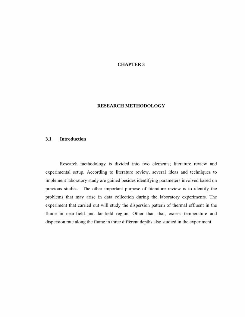
Photo 4.1: Trajectory of thermal effluent discharge in the channel (Qe= 0.05 liter/s,
Qa=10 liter/s)
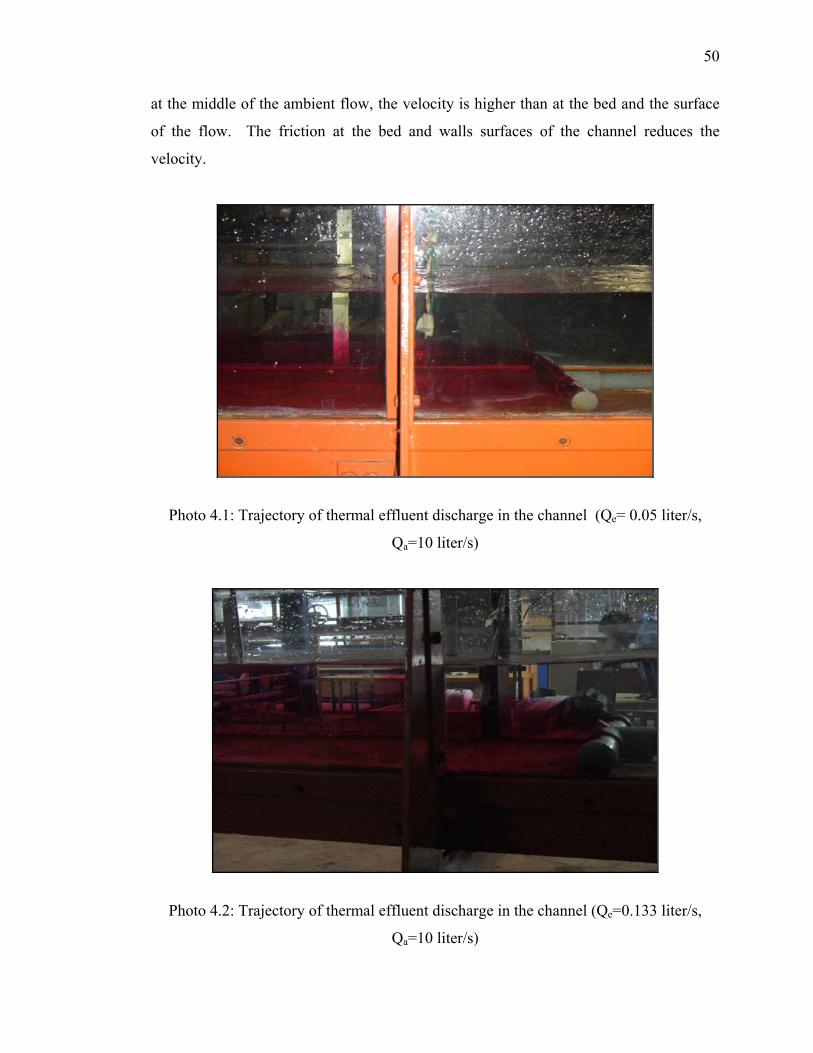
Photo 4.2: Trajectory of thermal effluent discharge in the channel (Qe=0.133 liter/s,
Qa=10 liter/s)

51
Based from Photo 4.1 and 4.2, it can be seen that for different volume of thermal
effluent discharged, the trajectory is different. For larger volume of thermal effluent, the
thermal effluent is trajected higher right after discharged into the ambient flow for the
same ambient flow velocity. Thus, the temperature is higher at the surface right after the
multi-port diffuser for the higher volume of thermal effluent.
Meanwhile for the smaller volume of the thermal effluent, the trajectoty of the
thermal effluent is lower. Thus, the surface temperature is lower right after the discharge
as the thermal effluent is being drifted by the ambient flow furher downstream before
reaching surface.
4.4 Digital Particle Image Velocimetry (DPIV) Method
The velocity vectors of the ambient flow can be determined by using Digital
Particle Image Velocimetry (DPIV) method. DPIV requires the projection of a laser
sheet onto the flow field at successive time intervals and the subsequent capturing of the
images detailing the position of seeding particles that reflect the laser light. Through
cross- correlation of two successive images in MATLAB software using correlation of
URAPIV file, the velocity vectors of the flume can be determined.
Figure 4.2a and Figure 4.2b show the velocity vectors for ambient flow rates of
20 liter/s and 10 liter/s, respectively. In the experiment, it is clearly seen that the water
particles move randomly in the flume. This indicates that the ambient flow is in
turbulent condition. This finding supports the calculated Reynolds number as described
in section 4.2, where ambient flow is turbulent condition.

52
Figure 4.2a: Velocity vectors using DPIV method for ambient flow of Qa of 20 liter/s
Figure 4.2b: Velocity vectors using DPIV method for ambient flow of Qa of 10 liter/s.

53
4.5 Effluent Dispersion Patterns
The cross-sectional effluent dispersion patterns for the cross-flow discharges are
illustrated from temperature difference (∆T) at every station. Temperature difference in
the mixed water is caused by density stratification between the ambient flow and the
effluent discharged. In the experiment, there are five stations measuring mixed water
temperature difference in the channel. The stations are located at x0/d = 0, x1/d = 30,
x2/d = 70, x3/d = 110 dan x4/d = 150. Based on calculated ∆T, isotherm lines are plotted
to observe effluent dispersion patterns along the channel.
The discussion of the dispersion pattern is divided into two zones; the near-field
and far-field region. For the near-field region, the discussion is at station x/d=30.
Meanwhile station x/d=110 is used for far-field region discussion. The dispersion pattern
figures are developed using software Surfer 32.
4.5.1 Dispersion Pattern in Near-Field (x/d=30)
Station x/d = 30 is selected to study the behaviour effluent dispersion in the near-
field region. Figures 4.3a shows cross-sectional temperature difference using isotherm
lines at x/d = 30 for Qe of 0.05 liter/s. Meanwhile, Figure 4.3b shows cross-sectional
effluent dispersion patterns at x/d = 30 for higher Qe of 0.133 liter/s. The ambient flow
rate for both figures is 20 liter/s. In Figure 4.3a, heated water moves to the surface of
the channel and disperse uniformly. Figure 4.3b also displays similar phenomenon
where the heated water moves to the surface of the channel but not well-dispersed.

54
The movement of the thermal effluent to the top of the channel is known as
positive buoyancy, where fluid with less density (i.e. heated water) moves upward
(Fischer et. al, 1979). This phenomenon results water temperature at surface is higher
than the temperature at the bottom of the channel. Both of the figures show that thermal
effluent starts to disperse in the channel when reaches x/d = 30.
In the Figure 4.3a, the highest temperature difference is 0.7 0C, while the lowest
is 0 0C. Meanwhile in Figure 4.3b, the highest temperature difference is at the bottom of
the channel with 0.28 °C and the lowest temperature difference is at the top side of the
channel with temperature difference of 0 °C. Higher temperature difference at the
bottom of the channel for Qe of 0.133 liter/s is due to the higher volume of thermal
effluent discharged into the channel as compared to for the case of Qe of 0.05 liter/s.
8.00 10.00 12.00 14.00 16.00 18.00
4.00
6.00
8.00
10.00
0.00
0.05
0.10
0.15
0.20
0.25
0.30
0.35
0.40
0.45
0.50
0.55
0.60
0.65
0.70
y/d
z/d
Temperature Scale
Figure 4.3a : Cross-sectional ∆T (in 0C) at x/d = 30 for Qa = 20.0 liter/s and Qe = 0.05
liter/s

55
8.00 10.00 12.00 14.00 16.00 18.00
4.00
6.00
8.00
10.00
0.00
0.02
0.04
0.06
0.08
0.10
0.12
0.14
0.16
0.18
0.20
0.22
0.24
0.26
0.28
y/d
z/d
Temperature Scale
Figure 4.3b : Cross-sectional ∆T (in 0C) at x/d = 30 for Qa = 20.0 liter/s and Qe = 0.133
liter/s
Meanwhile, Figures 4.4a and 4.4b show effluent dispersion temperature
difference for ambient flow rate of 10 liter/s using isotherm lines at x/d at 30 for Qe of
0.05 liter/s and 0.133 liter/s, respectively. Figure 4.4a shows that the heated water
moves to the middle layer of the channel while in Figure 4.4b the heated water remains
at the bottom of the channel.
The movement of the thermal effluent to mid-flow depth of the channel in
Figure 4.4a shows that positive buoyancy has influenced the dispersion pattern, where
fluid with less density (i.e. heated water) moves upwards to the water surface. However,
because of the smaller effluent flow rate, the dispersion rate decreases. In other words,
the dispersion rate is directly proportional to mass flow rate.
fluid with less density (i.e. heated water) moves upwards to the water surface. However,
because of the smaller effluent flow rate, the dispersion rate decreases. In other words,
the dispersion rate is directly proportional to mass flow rate.

56
Both of the figures show that thermal effluent start to disperse in the channel at
x/d = 30. In Figure 4.4a, the highest temperature difference is 0.65 0C while the lowest
is 0.15 0C. Based on Figure 4.4b, the highest temperature difference is 0.480C while the
lowest is 0.08 0C. The thermal effluent is still at the bottom of the channel in Figure 4.4b
as the volume of thermal effluent is bigger. Longer distance is needed to dilute the
thermal effluent.
8.00 10.00 12.00 14.00 16.00 18.002.00
4.00
6.00
8.00
0.15
0.20
0.25
0.30
0.35
0.40
0.45
0.50
0.55
0.60
0.65
y/d
z/d
Temperature Scale
Figure 4.4a : Cross-sectional ∆T (in 0C) at x/d = 30 for Qa = 10.0 liter/s and Qe = 0.05
liter/s

57
8.00 10.00 12.00 14.00 16.00 18.002.00
4.00
6.00
8.00
0.08
0.13
0.18
0.23
0.28
0.33
0.38
0.43
0.48
y/d
z/d
Temperature Scale
Figure 4.4b : Cross-sectional ∆T (in 0C) at x/d = 30 for Qa = 10.0 liter/s and Qe = 0.133
liter/s
4.5.2 Dispersion Pattern in Far-Field (x/d = 110)
Figures 4.5a shows isothermal lines to visualise the thermal effluent dispersion
for Qa of 20 liter/s at far-field region for Qe of 0.05 liter/s Meanwhile, Figure 4.5b
shows cross-sectional effluent dispersion patterns at x/d of 110 for Qe of 0.133 liter/s.
The highest temperature difference in Figure 4.5a is located at the top of the channel
which is 0.5 0C while the lowest temperature difference is 0 0C at bottom of the channel.
From observation, the result shows that minimum thermal stratification occurs in the far-
field region.
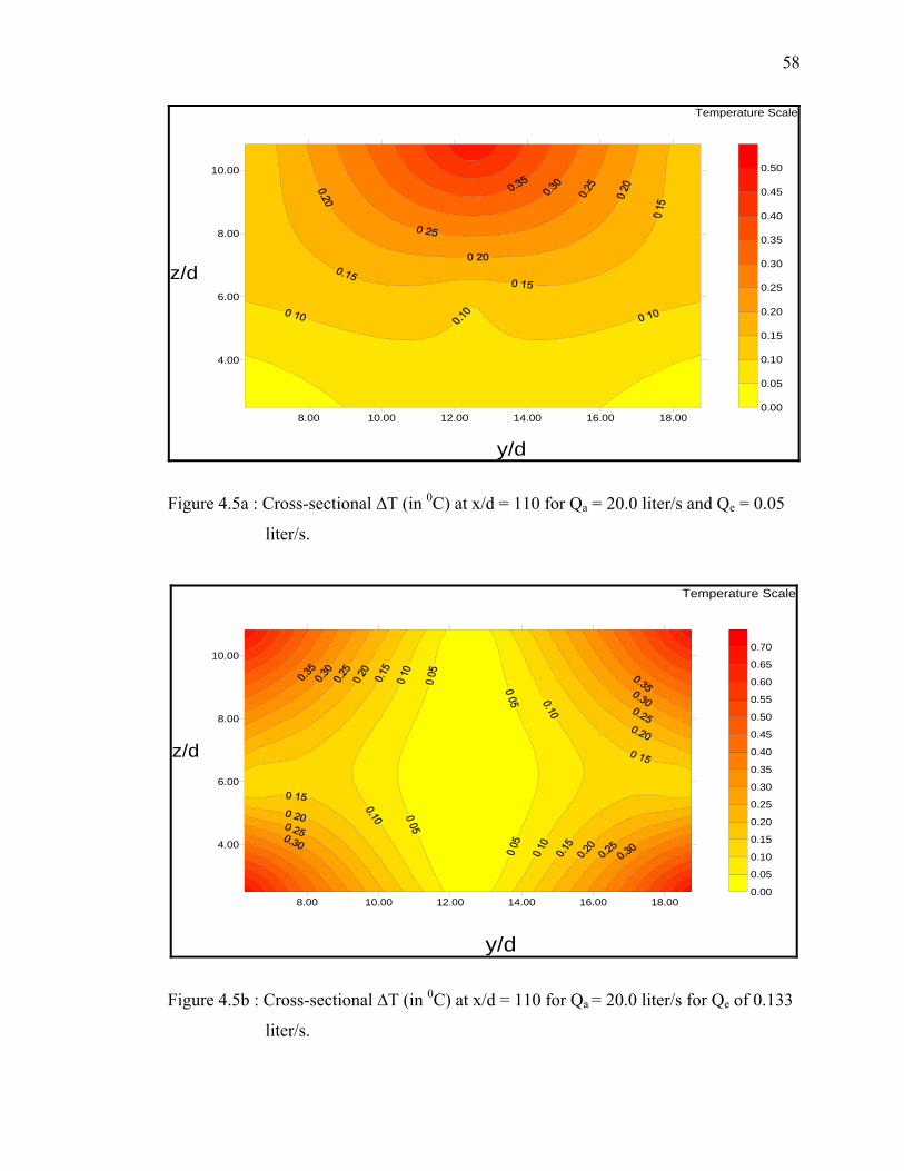
58
8.00 10.00 12.00 14.00 16.00 18.00
4.00
6.00
8.00
10.00
0.00
0.05
0.10
0.15
0.20
0.25
0.30
0.35
0.40
0.45
0.50
y/d
z/d
Temperature Scale
Figure 4.5a : Cross-sectional ∆T (in 0C) at x/d = 110 for Qa = 20.0 liter/s and Qe = 0.05
liter/s.
8.00 10.00 12.00 14.00 16.00 18.00
4.00
6.00
8.00
10.00
0.00
0.05
0.10
0.15
0.20
0.25
0.30
0.35
0.40
0.45
0.50
0.55
0.60
0.65
0.70
y/d
z/d
Temperature Scale
Figure 4.5b : Cross-sectional ∆T (in 0C) at x/d = 110 for Qa = 20.0 liter/s for Qe of 0.133
liter/s.

59
Consequently, in Figure 4.5b, the highest temperature difference is 0.7 0C at both
sides corners of the channel while the lowest temperature difference is 0 0C in the
middle of the channel. At the centre of the flume, the velocity is higher compared to at
the side of the flume. As a result, the mixing process at the centre of the flume is
completed. The mixing by the flume wall is still incomplete as the velocity is smaller.
This is caused by the mixing in this area is influenced by friction effect between the
heated effluents with the side of the channel.
Meanwhile Figures 4.6a and 4.6b show isothermal lines to visualise the thermal
effluent dispersion for ambient flow rate of 10 liter/s at x/d = 110 for Qe of 0.05 liter/s
and Qe of 0.133 liter/s, respectively. Both figures show that mixing process at that
station is almost complete. The highest temperature difference in Figure 4.6a is 1.00C
while the lowest temperature difference is 0 0C at both sides of the channel. Referring
Figure 4.6b, the highest temperature difference is 1.4 0C while the lowest temperature
difference is 0 0C. From observation, the result shows that positive buoyancy has
influenced the dispersion .

60
8.00 10.00 12.00 14.00 16.00 18.002.00
4.00
6.00
8.00
0.00
0.10
0.20
0.30
0.40
0.50
0.60
0.70
0.80
0.90
1.00
y/d
z/d
Temperature Scale
Figure 4.6a : Cross-sectional ∆T (in 0C) at x/d = 110 for Qa = 10.0 liter/s and Qe = 0.05
liter/s
8.00 10.00 12.00 14.00 16.00 18.002.00
4.00
6.00
8.00
0.00
0.20
0.40
0.60
0.80
1.00
1.20
1.40
y/d
z/d
Temperature Scale
Figure 4.6b : Cross-sectional ∆T (in 0C) at x/d = 110 for Qa = 10.0 liter/s and Qe = 0.133
liter/s.

61
Based on the observation of cross-sectional temperature differences in the
channel, some conclusions can be made. The dispersion of thermal effluent in high
ambient flow rate is higher due to its high velocity. Meanwhile, for larger volume of
thermal effluent discharged, the dispersion rate is lower. This occurs due to the
longitudinal distance needed in cooling the thermal effluent is longer. The difference in
density between the ambient flow and thermal effluent discharge creates thermal
stratification in the open channel flow.
4.6 Excess Temperature, ∆T/Te
Analysis on the temperature difference, ∆T is concentrated on two different
ambient flow rates, Qa of 20.0 liter/s and 10.0 liter/s and two different thermal effluent
flow rates, Qe of 0.133 liter/s and 0.05 liter/s. The ratio between the thermal effluent
flow rates is 2.67. Subsequently, ∆T obtained in the analysis is normalised to acquire
excess temperature, ∆T/Te as in equation 2.10.
The study of excess temperature is carried out in three different flow depths
known as lower layer, middle layer and upper layers. Lower layer of the flow represents
z/H of 0.2 while middle layer corresponds to z/H of 0.4. The upper layer stands for z/H
of 0.8.

62
4.6.1 Effect of Different Qe on Excess Temperature for A Constant Qa of 20 liter/s
Figure 4.7 shows longitudinal excess temperature profile for Qa of 20 liter/s at
lower layer of flow. At x/d of 0, for Qe of 0.05 liter/s and Qe of 0.133 liter/s, excess
temperature is high as the thermometer detects the mass of heated water discharged into
the channel. Then, excess temperature decreases since thermal effluent is cooling as it
moves along the channel. This phenomenon arises as mixing occurs between thermal
effluent and ambient flow. However, excess temperature for Qe of 0.133 liter/s is high as
the mass of thermal effluent discharge is higher compared to Qe of 0.05 liter/s. The
excess temperature equations for Qe of 0.05 liter/s and Qe of 0.133 liter/s at lower layer
of flow are as follow respectively :
eTT∆ = 1.285 x 10⁻⁶ ⎟
⎠⎞
⎜⎝⎛
dx 2 - 2.62 x 10⁻⁴ ⎟
⎠⎞
⎜⎝⎛
dx + 17.908 x 10⁻³ (4.1)
eTT∆ = 1.138 x 10⁻⁶ ⎟
⎠⎞
⎜⎝⎛
dx 2 - 2.772 x 10⁻⁴ ⎟
⎠⎞
⎜⎝⎛
dx + 18.565 x 10⁻³ (4.2)
Figure 4.8 shows longitudinal excess temperature profile for Qa of 20 liter/s at
middle layer of flow. For Qe of 0.05 liter/s, at x/d of 0, excess temperature is low with
zero value because the thermometer does not detect the mass of heated water. However,
as thermal effluent moves further downstream, excess temperature increases indicates
that mass of thermal effluent moves upwards. The rising of thermal effluent in the
receiving water is known as positive buoyancy. Afterward, excess temperature decreases
along the channel length as the mixing between thermal effluent and ambient flow
continue to take place. Equation 4.3 shows excess temperature for Qe of 0.05 liter/s at
middle layer of flow for Qa of 20 liter/s.
eTT∆ = –1.293 x 10⁻⁶ ⎟
⎠⎞
⎜⎝⎛
dx 2 + 1.872 x 10⁻⁴ ⎟
⎠⎞
⎜⎝⎛
dx + 2.171 x 10⁻³ (4.3)

63
For Qe of 0.133 liter/s, at x/d of 0, excess temperature is low because the
thermometer does not detect the mass of heated water. However, as thermal effluent
moves further downstream, excess temperature increases. Excess temperatures continue
to increase due to large quantity of thermal effluent discharges in the channel. The
excess temperature equation for Qe of 0.133 liter/s at upper layer of flow is as shown in
equation 4.4.
eTT∆ = –2.305 x 10⁻⁷ ⎟
⎠⎞
⎜⎝⎛
dx 2 + 86.295 x 10⁻⁶ ⎟
⎠⎞
⎜⎝⎛
dx + 6.492 x 10⁻⁴ (4.4)
Figure 4.9 shows longitudinal excess temperature profile for Qa of 20 liter/s at
upper layer of flow. For Qe of 0.05 liter/s, at x/d of 0, excess temperature is low because
the thermometer does not detect the mass of heated water as the heated water mass still
flow at the lower layer of the flow. However, as thermal effluent move further, excess
temperature increases. The tendency of thermal effluent to rise in the receiving water is
generated by the density gradient. The fluctuation of data for Qe of 0.05 liter/s is mainly
caused by the turbulent flow of the ambient. Equation 4.5 shows excess temperature for
Qe of 0.05 liter/s at upper layer of flow for Qa of 20 liter/s.
eTT∆ = – 4.004 x 10⁻⁷ ⎟
⎠⎞
⎜⎝⎛
dx 2+ 1.005 x 10⁻⁴ ⎟
⎠⎞
⎜⎝⎛
dx + 5.197 x 10⁻³ (4.5)
At x/d of 0, for Qe of 0.133 liter/s, excess temperature is low because the
thermometer does not detect the mass of heated water as mentioned earlier for Qe of 0.05
liter/s. However, as thermal effluent move further downstream, excess temperature
increases to show mass of heated water moves upwards. Again, positive buoyancy plays
a role where the thermal effluent rises upward in the receiving water. Excess
temperature continues to increase due to the large quantity of thermal effluent
discharged into the channel. The fluctuation of excess temperature for Qe of 0.133 liter/s
shows the presence of turbulence flow in the channel. The following equation 4.6
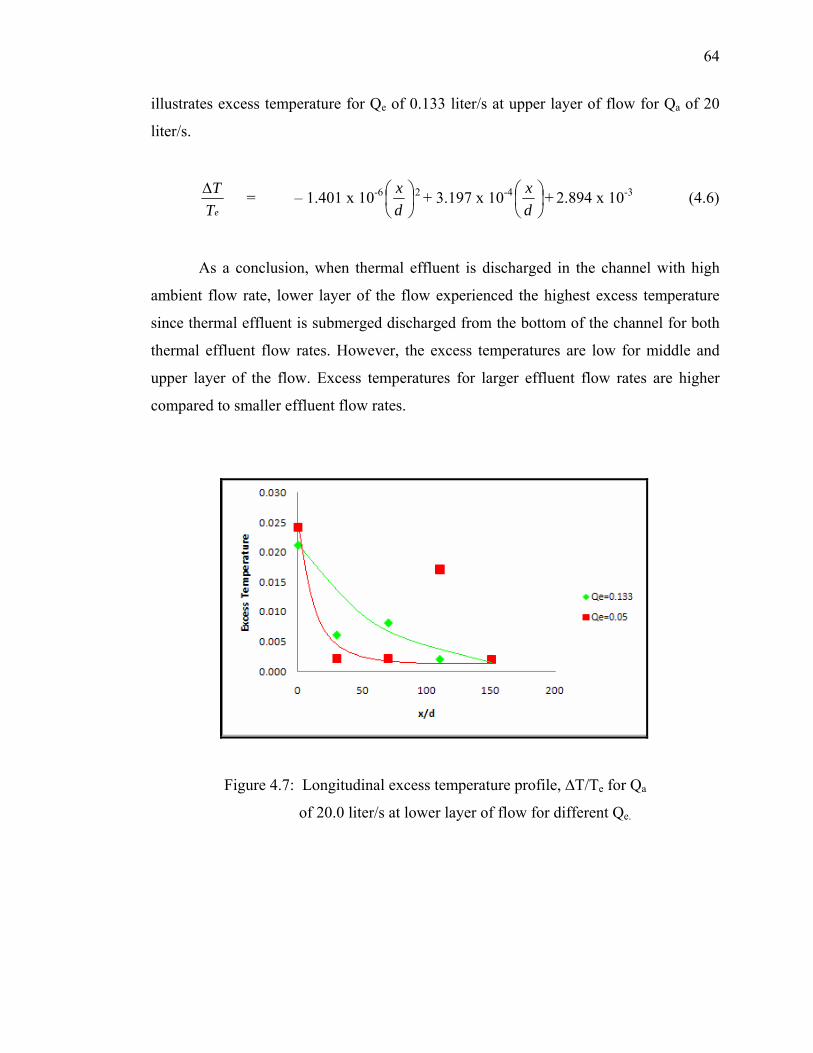
64
illustrates excess temperature for Qe of 0.133 liter/s at upper layer of flow for Qa of 20
liter/s.
eTT∆ = – 1.401 x 10⁻⁶ ⎟
⎠⎞
⎜⎝⎛
dx 2 + 3.197 x 10⁻⁴ ⎟
⎠⎞
⎜⎝⎛
dx + 2.894 x 10⁻³ (4.6)
As a conclusion, when thermal effluent is discharged in the channel with high
ambient flow rate, lower layer of the flow experienced the highest excess temperature
since thermal effluent is submerged discharged from the bottom of the channel for both
thermal effluent flow rates. However, the excess temperatures are low for middle and
upper layer of the flow. Excess temperatures for larger effluent flow rates are higher
compared to smaller effluent flow rates.
Figure 4.7: Longitudinal excess temperature profile, ∆T/Te for Qa
of 20.0 liter/s at lower layer of flow for different Qe.

65
Figure 4.8 : Longitudinal excess temperature profile, ∆T/Te for Qa
of 20.0 liter/s at middle layer of flow for different Qe.
Figure 4.9 : Longitudinal excess temperature profile, ∆T/Te for Qa
of 20.0 liter/s at upper layer of flow for different Qe.

66
4.6.2 Effect of Different Qe on Excess Temperature for A Constant Qa of 10 liter/s
Figure 4.10 shows longitudinal excess temperature profile for Qa of 10 liter/s at
lower layer of flow. For Qe of 0.05 liter/s and 0.133 liter/s, at x/d of 0, excess
temperature is high because thermometer detects the mass of heated water. Excess
temperature decreases with channel length as mixing between thermal effluent and
ambient flow occurs and reduces the water temperature. Equations 4.7 and 4.8 show
excess temperature equations for Qe of 0.05 liter/s and Qe of 0.133 liter/s at lower layer
of flow for Qa of 10 liter/s.
eTT∆ = 1.037 x 10⁻⁶ ⎟
⎠⎞
⎜⎝⎛
dx 2 - 2.42 x 10⁻⁴ ⎟
⎠⎞
⎜⎝⎛
dx + 0.024 (4.7)
eTT∆ = – 2.88 x 10⁻⁷ ⎟
⎠⎞
⎜⎝⎛
dx 2- 41.291 x 10⁻⁶ ⎟
⎠⎞
⎜⎝⎛
dx + 18.5 x 10⁻³ (4.8)
Figure 4.11 shows longitudinal excess temperature profile for Qa of 10 liter/s at
middle layer of flow. For Qe of 0.05 liter/s and 0.133 liter/s, at x/d of 0, excess
temperature is high as the thermometer detected the mass of heated water. Excess
temperature decreases with channel length as mixing occurs that reduced the water
temperature. Excess temperature equations for Qe of 0.05 liter/s and Qe of 0.133 liter/s at
middle layer of flow are as follow respectively:
eTT∆ = 2.58 x 10⁻⁶ ⎟
⎠⎞
⎜⎝⎛
dx 2 – 5.909 x 10⁻⁴ ⎟
⎠⎞
⎜⎝⎛
dx + 0.037 (4.9)
eTT∆ = – 1.401 x 10⁻⁶ ⎟
⎠⎞
⎜⎝⎛
dx 2 + 3.197 x 10⁻⁴ ⎟
⎠⎞
⎜⎝⎛
dx + 16.79 x 10⁻³ (4.10)
Figure 4.12 shows longitudinal excess temperature profile for Qa of 10 liter/s at
upper layer of flow. For Qe of 0.05 liter/s, at x/d of 0, excess temperature is low with

67
zero value as the thermometer does not detect the mass of heated water. However, as
thermal effluent moves further downstream, excess temperature increases that shows
thermal effluent moves upwards. Again, the tendency of thermal effluent to rise in the
receiving water is known as positive buoyancy. Equation of excess temperature for Qe of
0.05 liter/s at upper layer of flow is as follow:
eTT∆ = – 1.249 x 10⁻⁶ ⎟
⎠⎞
⎜⎝⎛
dx 2 + 2.244 x 10⁻⁴ ⎟
⎠⎞
⎜⎝⎛
dx - 2.634 x 10⁻⁴ (4.11)
For Qe of 0.133 liter/s, at x/d of 0, excess temperature is low with zero value
because the thermometer does not detect the mass of heated water. However, as thermal
effluent move further downstream, excess temperature increases as the thermal effluent
moves upwards. The excess continue to increase due to the large mass of thermal
effluent discharges into the channel. Equation 4.12 shows excess temperature equation
for Qe of 0.133 liter/s at upper layer of flow.
eTT∆ = – 1.401 x 10⁻⁶ ⎟
⎠⎞
⎜⎝⎛
dx 2 + 3.197 x 10⁻⁴ ⎟
⎠⎞
⎜⎝⎛
dx + 2.894 x 10⁻³ (4.12)
Overall, in low ambient flow rate, as thermal effluent is discharged in the
channel, lower layer of the flow experienced the highest excess temperature as thermal
effluent is discharged at the bottom of the channel for both thermal effluent flow rates.
However, the excess temperatures are low in middle and upper layers of the flow.
Excess temperatures resulted from high effluent flow rates are larger compared to low
thermal effluent flow rates.

68
Figure 4.10 : Longitudinal excess temperature profile, ∆T/Te for Qa
of 10.0 liter/s at lower layer of flow for different Qe.
Figure 4.11 : Longitudinal excess temperature profile, ∆T/Te for Qa
of 10.0 liter/s at middle layer of flow for different Qe.

69
Figure 4.12 : Longitudinal excess temperature profile, ∆T/Te for Qa
of 10.0 liter/s at upper layer of flow for different Qe.
4.6.3 Effect of Different Qa on Excess Temperature for A Constant Qe of 0.133
liter/s
Figure 4.13 shows longitudinal excess temperature profile for Qe of 0.133 liter/s
at lower layer of flow. For Qa of 20 liter/s and 10 liter/s, excess temperature is high
because thermometer at x/d of 0 detects the mass of heated water. Excess temperature
decreases along the channel length as mixing between thermal effluent and ambient flow
takes place which reduces the water temperature.
Figure 4.14 shows longitudinal excess temperature profile for Qe of 0.133 liter/s
at middle layer of flow. For Qa of 20 liter/s, excess temperature is low with zero value
the mass of heated water is not detected by the thermometer. However, as thermal
effluent moves further downstream, the excess temperature increases since the thermal

70
mass moves upwards. Excess temperatures keep increasing as a result of the large
thermal effluent quantity discharged in the channel.
For Qa of 10 liter/s, at x/d of 0, excess temperature is high as the thermometer
detects the mass of heated water. Excess temperature decreases with channel length
when mixing occurs between the ambient flow and the thermal effluent.
Figure 4.15 shows longitudinal excess temperature profile for Qe of 0.133 liter/s
at upper layer of flow. For Qa of 20 liter/s and 10 liter/s, at x/d of 0, excess temperature
is low because the thermometer does not detect the mass of heated water. However, as
thermal effluent moves further, excess temperature increases as thermal effluent moves
to the ambient flow surface. This behaviour of is known as positive buoyancy. Excess
temperature continues to increase due to large quantity of thermal effluent discharged
into the channel.
The analysis on effect of different Qa on excess temperature for a constant high
thermal effluent flow rate comes out with the following conclusion. In high thermal
effluent flow rate, lower layer of the flow experiences the highest excess temperature
since thermal effluent is discharged at the bottom of the channel for both ambient flow
rates studied. However, the excess temperatures are low for middle and upper layer of
the flow. Excess temperature for low ambient flow rate is higher compared to high
ambient flow rates due to less volume of cold water to mix (cool) the heated water mass.

71
Figure 4.13 : Longitudinal excess temperature profile, ∆T/Te for Qe
of 0.133 liter/s at lower layer of flow for different Qa.
Figure 4.14 : Longitudinal excess temperature profile, ∆T/Te for Qe
of 0.133 liter/s at middle layer of flow for different Qa.

72
Figure 4.15 : Longitudinal excess temperature profile, ∆T/Te for Qe
of 0.133 liter/s at upper layer of flow for different Qa.
4.6.4 Effect of Different Qa on Excess Temperature for A Constant Qe of 0.05
liter/s
Figure 4.16 shows longitudinal excess temperature profile for Qe of 0.05 liter/s at
lower layer of flow. For Qa of 20 liter/s and 10 liter/s, at x/d of 0, excess temperature is
high because thermometer detects the mass of heated water. Excess temperature
decreases with channel as mixing between thermal effluent and ambient flow occurs and
reduces the water temperature.
Figure 4.17 shows longitudinal excess temperature profile for Qe of 0.05 liter/s at
middle layer of flow. For Qa of 20 liter/s, at x/d of 0, excess temperature is low as the
mass of heated water is not detected by the thermometer. However, as thermal effluent
moves further, excess temperature increases as the thermal effluent moves upwards.
Positive buoyancy is indicated by the rising of thermal effluent in the flume. Afterwards,
73
the excess temperature decreases with the channel length as mixing between thermal
effluent and ambient flow occurs.
Meanwhile, for Qa of 10 liter/s, at x/d of 0, excess temperature is high because
thermometer detects the mass of heated water. Excess temperature decreases with
channel length as mixing occurs between ambient flow and thermal effluent, thus
reducing the water temperature.
Figure 4.18 shows longitudinal excess temperature profile for Qe of 0.05 liter/s at
upper layer of flow. For Qa of 20 liter/s, at x/d of 0, excess temperature is low as the
thermometer does not detect the mass of heated water. However, as thermal effluent
moves further, excess temperature increases, signifying that the thermal effluent rises to
the surface ambient flow. Excess temperature decreases in a region far from multi-port
diffuser because mixing occurs between thermal effluent and ambient flow. The
fluctuation of excess temperature shows that turbulent flow affected the mixing process.
For Qa of 10 liter/s, at x/d of 0, excess temperature is low because the
thermometer does not detect the mass of heated water. However, as thermal effluent
moves further, excess temperature increases because the thermal effluent moves
upwards due to the temperature gradient between thermal effluent discharged and
ambient flow. Afterwards, excess temperature decreases because mixing between
thermal effluent and ambient flow takes place.
In general, lower layer of the flow experiences the highest thermal impact due to
the bottom discharges of effluent for both ambient flow rates in low thermal effluent
flow rate. However, the excess temperatures are low for middle and upper layer of the

74
flow. Excess temperatures for low ambient flow rates are higher compared to high
ambient flow rate due to less volume of cold water to cool the heated water mass.
Figure 4.16 : Longitudinal excess temperature profile, ∆T/Te for Qe
of 0.05 liter/s at lower layer of flow for different Qa.
Figure 4.17 : Longitudinal excess temperature profile, ∆T/Te for Qe
of 0.05 liter/s at middle layer of flow for different Qa.

75
Figure 4.18 : Longitudinal excess temperature profile, ∆T/Te for Qe
of 0.05 liter/s at upper layer of flow for different Qa.
4.7 Dispersion Rate, KT
Analysis on the effluent dispersion rate, KT is important in determining the
efficiency of pipe diffuser system in the experiment. Dispersion rate always inversely
proportion to the excess temperature. A small changes of temperatures gives higher
dispersion rates. Ambient flow velocity and distance from multiport diffuser influence
dispersion rate in open channel. from KT can be calculated using equation 2.11.
The analysis of dispersion rate is carried out three different flow depths known as
lower layer, middle layer and upper layer of the flow. Lower layer of the flow represents
the value z/H of 0.2 while middle layer corresponds to z/H of 0.4. Meanwhile, upper
layer stands for z/H of 0.8.

76
The profile of calculated KT is plotted along the channel and the results are
discussed in the following sections.
4.7.1 Effect of Different Qe on Dispersion Rate for A Constant Qa of 20 liter/s
Figure 4.19 shows longitudinal dispersion rate profile for Qa of 20 liter/s at lower
layer of flow. For Qe of 0.05 liter/s and 0.133 liter/s, as the excess temperature
decreases along the channel length, the momentum ratio between ambient flow and
thermal effluent discharged increases. Momentum is defined as the product of the mass
of a body and its velocity ( L. Mott, 1990). Momentum ratio influences the rising of
dispersion rate. The dispersion rate for Qe of 0.05 liter/s are higher compared to
dispersion rate for Qe of 0.133 liter/s because the momentum ratio for Qe of 0.05 liter/s is
higher compared to momentum ratio for Qe of 0.133 liter/s. The dispersion rate
equations for Qe of 0.05 liter/s and Qe of 0.133 liter/s at lower layer of flow are as follow
respectively:
KT = – 6.059 x 10⁻⁴ ⎟⎠⎞
⎜⎝⎛
dx 2 + 1.403 ⎟
⎠⎞
⎜⎝⎛
dx + 76.774 (4.13)
KT = 27.279 x 10⁻⁴ ⎟⎠⎞
⎜⎝⎛
dx 2 + 1.081 ⎟
⎠⎞
⎜⎝⎛
dx + 22.304 (4.14)
Figure 4.20 shows longitudinal dispersion rate profile for Qa of 20 liter/s at
middle layer of flow. Again, for Qe of 0.05 liter/s and 0.133 liter/s, the momentum ratio
between ambient flow and thermal effluent discharged increases because the excess
temperatures decreases along the channel length. Definition of momentum is the product
of the mass of a body and its velocity. As momentum ratio increases, dispersion rate also
increases. The dispersion rate for Qe of 0.05 liter/s are higher compared to dispersion

77
rates for Qe of 0.133 liter/s because the momentum ratio for Qe of 0.05 liter/s is higher
compared to momentum ratio for Qe of 0.133 liter/s. Equations 4.15 and 4.16 show
dispersion rate equations for Qe of 0.05 liter/s and 0.133 liter/s at middle layer of flow
respectively.
KT = 8.09 x 10⁻³ ⎟⎠⎞
⎜⎝⎛
dx 2 – 52.216 x 10⁻³ ⎟
⎠⎞
⎜⎝⎛
dx + 13.696 (4.15)
KT = – 10.801 x 10⁻³ ⎟⎠⎞
⎜⎝⎛
dx 2 + 1.762 ⎟
⎠⎞
⎜⎝⎛
dx + 22.233 (4.16)
Figure 4.21 shows longitudinal dispersion rate profile for Qa of 20 liter/s at upper
layer of flow. For Qe of 0.05 liter/s and 0.133 liter/s, as the excess temperatures
increases along the channel length, the momentum ratio between ambient flow and
thermal effluent discharged decreases. Momentum is the product of the mass of a body
and its velocity. The decreasing of momentum ratio influenced the decreasing of
dispersion rate. The dispersion rates for Qe of 0.05 liter/s are lower compared to
dispersion rates for Qe of 0.133 liter/s due to turbulence generated by strong velocity of
the jet discharged from the diffuser. The dispersion rate equations for Qe of 0.05 liter/s
and Qe of 0.133 liter/s at lower layer of flow for Qa of 20 liter/s are as follow:
KT = 8.092 x 10⁻⁴ ⎟⎠⎞
⎜⎝⎛
dx 2 - 0.448 ⎟
⎠⎞
⎜⎝⎛
dx + 89.926 (4.17)
KT = -31.96 x 10⁻³ ⎟⎠⎞
⎜⎝⎛
dx 2 + 5.05 ⎟
⎠⎞
⎜⎝⎛
dx + 5.441 (4.18)
Based on the analysis of effect of different Qe on dispersion rate for a constant
high ambient flow rate, the dispersion rates for lower thermal effluent flow rate are
higher compared to higher thermal effluent flow rate in high ambient flow rate because
the momentum ratio for lower thermal effluent flow rate is higher than momentum ratio
for higher thermal effluent flow rate.

78
Figure 4.19 : Longitudinal dispersion rate profile, KT for Qa of
20.0 liter/s at lower layer of flow for different Qe.
Figure 4.20 : Longitudinal dispersion rate profile, KT for Qa of
20.0 liter/s at middle layer of flow for different Qe.

79
Figure 4.21 : Longitudinal dispersion rate profile, KT for Qa of
20.0 liter/s at upper layer of flow for different Qe.
4.7.2 Effect of Different Qe on Dispersion Rate for A Constant Qa at 10 liter/s
Figure 4.22 shows longitudinal dispersion rate profile for Qa of 10 liter/s at lower
layer of flow. For Qe of 0.05 liter/s and 0.133 liter/s, as the excess temperature
decreases along the channel length, the momentum ratio increases. Momentum is the
product of the mass of a body and its velocity. The rising of momentum ratio influence
the rising of dispersion rate. The dispersion rate for Qe of 0.05 liter/s are higher
compared to dispersion rate for Qe of 0.133 liter/s because the momentum ratio for Qe of
0.05 liter/s is higher compared to momentum ratio for Qe of 0.133 liter/s. The dispersion
rate equations for Qe of 0.05 liter/s and Qe of 0.133 liter/s at lower layer of flow are as
shown in equation 4.19 and 4.20 respectively.
KT = – 1.547 x 10⁻³ ⎟⎠⎞
⎜⎝⎛
dx 2 + 0.526 ⎟
⎠⎞
⎜⎝⎛
dx + 12.503 (4.19)

80
KT = 19.646 x 10⁻³ ⎟⎠⎞
⎜⎝⎛
dx 2 – 1.811 ⎟
⎠⎞
⎜⎝⎛
dx + 47.479 (4.20)
Figure 4.23 shows longitudinal dispersion rate profile for Qa of 10 liter/s at
middle layer of flow. For Qe of 0.05 liter/s and 0.133 liter/s, as the excess temperatures
decreases along the channel length, the momentum ratio increases. Momentum ratio is
proportional to dispersion rate. The rising of momentum ratio influence the rising of
dispersion rate. The dispersion rate for Qe of 0.05 liter/s are higher compared to
dispersion rate for Qe of 0.133 liter/s because the momentum ratio for Qe of 0.05 liter/s is
higher compared to momentum ratio for Qe of 0.133 liter/s. The dispersion rate
equations for Qe of 0.05 liter/s and Qe of 0.133 liter/s at lower layer of flow for Qa of 10
liter/s are as follow:
KT = 2.58 x 10⁻⁶ ⎟⎠⎞
⎜⎝⎛
dx 2 - 5.909x 10⁻⁴ ⎟
⎠⎞
⎜⎝⎛
dx + 0.037 (4.21)
KT = – 4.037 x 10⁻³ ⎟⎠⎞
⎜⎝⎛
dx 2 + 0.63 ⎟
⎠⎞
⎜⎝⎛
dx + 38.283 (4.22)
Figure 4.24 shows longitudinal dispersion rate profile for Qa of 10 liter/s at upper
layer of flow. For Qe of 0.05 liter/s and 0.133 liter/s, as the excess temperature
decreases along the channel length, the momentum ratio increases. Momentum is the
product of the mass of a body and its velocity. Again, the rising of momentum ratio
influence the rising of dispersion rate. The dispersion rate for Qe of 0.05 liter/s are lower
compared to dispersion rate for Qe of 0.133 liter/s due to turbulence generated by strong
velocity of the jet discharged from the diffuser. Equations 4.23 and 4.24 show dispersion
rate equations for Qe of 0.05 liter/s and Qe of 0.133 liter/s at upper layer of the flow.
KT = - 1.249 x 10⁻⁶ ⎟⎠⎞
⎜⎝⎛
dx 2 + 2.244 x 10⁻⁴ ⎟
⎠⎞
⎜⎝⎛
dx - 2.634 x 10⁻⁴ (4.23)

81
KT = - 22.477 x 10⁻³ ⎟⎠⎞
⎜⎝⎛
dx 2 + 3.346 ⎟
⎠⎞
⎜⎝⎛
dx + 19.44 (4.24)
As a conclusion, in low ambient flow rate, as thermal effluent is discharged in
the channel, the dispersion rate for lower thermal effluent flow rate are higher compared
to dispersion rate for higher thermal effluent flow rate because the momentum ratio for
lower thermal effluent flow rate is higher compared to momentum ratio for higher
thermal effluent flow rate.
Figure 4.22 : Longitudinal dispersion rate profile, KT for Qa of
10.0 liter/s at lower layer of flow for different Qe.

82
Figure 4.23 : Longitudinal dispersion rate profile, KT for Qa of
10.0 liter/s at middle layer of flow for different Qe.
Figure 4.24 : Longitudinal dispersion rate profile, KT for Qa of
10.0 liter/s at upper layer of flow for different Qe.

83
4.7.3 Effect of Different Qa on Dispersion Rate for A Constant Qe at 0.133 liter/s
Figure 4.25 shows longitudinal dispersion rate profile for Qe of 0.133 liter/s at
lower layer of flow. For Qa of 20 liter/s and 10 liter/s, as the excess temperature
decreases along the channel length, the momentum ratio increases. Momentum is
defined as the product of the mass of a body and its velocity. The rising of momentum
ratio influence the rising of dispersion rates. The dispersion rate for Qa of 20 liter/s is
higher than dispersion rates for Qa of 10 liter/s because the momentum ratio is higher
than momentum ratio for Qa of 10 liter/s.
Figure 4.26 shows longitudinal dispersion rate profile for Qe of 0.133 liter/s at
middle layer of flow. For Qa of 20 liter/s and 10 liter/s, as the excess temperature
decreases along the channel length, the momentum ratio increases. Momentum is the
product of the mass of a body and its velocity. The rising of momentum ratio influence
the rising of dispersion rate. The dispersion rates for Qa of 20 liter/s are higher than
dispersion rate for Qa of 10 liter/s because the momentum ratio is higher than
momentum ratio for Qa of 10 liter/s.
Figure 4.27 shows longitudinal dispersion rate profile for Qe of 0.133 liter/s at
upper layer of flow. For Qa of 20 liter/s and 10 liter/s, as the excess temperatures
increases along the channel length, the momentum ratio decreases. The decreasing of
momentum ratio influenced the decreasing of dispersion rates. The dispersion rate for Qa
of 20 liter/s are higher compared to dispersion rates for Qa of 10 liter/s because the
momentum ratio is higher compared to momentum ratio for Qa of 10 liter/s.
In general, as thermal effluent is discharged in the channel, the dispersion rates
for higher ambient flow rate are higher compared to dispersion rate for lower ambient

84
flow rate in high thermal effluent flow rate because the momentum ratio for higher
ambient flow rate is higher compared to momentum ratio for lower ambient flow rate.
Figure 4.25 : Longitudinal dispersion rate profile, KT for Qe of
0.133 liter/s at lower layer of flow for different Qa.
Figure 4.26 : Longitudinal dispersion rate profile, KT for Qe of
0.133 liter/s at middle layer of flow for different Qa.

85
Figure 4.27 : Longitudinal dispersion rate profile, KT for Qe of
0.133 liter/s at upper layer of flow for different Qa.
4.7.4 Effect of Different Qa on Dispersion Rate for A Constant Qe at 0.05 liter/s
Figure 4.28 shows longitudinal dispersion rate profile for Qe of 0.05 liter/s at
lower layer of flow. For Qa of 20 liter/s and 10 liter/s, as the excess temperature
decreases along the channel length, the momentum ratio increases. As momentum ratio
is proportional to the dispersion rate, the rising of momentum ratio influences the rising
of dispersion rate. The dispersion rate for Qa of 20 liter/s is higher compared to
dispersion rate for Qa of 10 liter/s because the momentum ratio for Qa of 20 liter/s is
higher than momentum ratio for Qa of 10 liter/s.
Figure 4.29 shows longitudinal dispersion rate profile for Qe of 0.05 liter/s at
middle layer of flow. Again, excess temperature is inversely proportional to the
momentum ratio. As the excess temperature decreases along the channel length, the
momentum ratio increases. The rising of momentum ratio influence the rising of

86
dispersion rate. Momentum is the product of the mass of a body and its velocity. The
dispersion rate for Qa of 20 liter/s is higher compared to dispersion rate for Qa of 10
liter/s because the momentum ratio for Qa of 20 liter/s is higher than momentum ratio for
Qa of 10 liter/s.
Figure 4.30 shows longitudinal dispersion rate profile for Qe of 0.05 liter/s at
upper layer of flow. As the excess temperatures increases along the channel length, the
momentum ratio decreases. The decreasing of momentum ratio influenced the
decreasing of dispersion rate. The dispersion rate for Qa of 20 liter/s are higher
compared to dispersion rate for Qa of 10 liter/s because the momentum ratio for Qa of 20
liter/s is higher compared to momentum ratio for Qa of 10 liter/s.
Overall, in lower thermal effluent flow rate, as thermal effluent is discharged in
the channel, the dispersion rate for higher ambient flow rate are higher compared to
dispersion rate for lower ambient flow rate because the momentum ratio for higher
ambient flow rate is higher compared to momentum ratio for lower ambient flow rate.
Figure 4.28 : Longitudinal dispersion rate profile, KT for Qe of
0.05 liter/s at lower layer of flow for different Qa.

87
Figure 4.29 : Longitudinal dispersion rate profile, KT for Qe of
0.05 liter/s at middle layer of flow for different Qa.
Figure 4.30 : Longitudinal dispersion rate profile, KT for Qe of
0.05 liter/s at upper layer of flow for different Qa.
88
4.8 Ambient Temperature Differences, ∆T with Dimensionless Time, t*
Data of temperature difference, ∆T is obtained as discussed earlier. The
dimensionless time, t* is used in the analysis in which t* is equal to:
t* = ett (4.25)
where t is time recorded for the experiment while te is time taken to discharge thermal
effluent into the channel which is 210 seconds.
Data is collected at x/d of 30 and x/d of 110 at three different flow depths, z/H
of 0.2 (lower layer of the flow), z/H of 0.4 (middle layer of the flow) and z/H of 0.8
(upper layer of the flow). However, the discussion is focused on z/H of 0.4 and y/d of
12.5 for flow rates of 20.0 liter/s and 10.0 liter/s.
Based on Figure 4.31 for Qa of 20 liter/s, maximum temperature difference
recorded is 0.5 at x/d of 30 which is located in near-field region. This condition happens
because station x/d of 30 is located near to the diffuser pipe and experiences the high
temperature of heated water. At x/d of 110, heated water has mixed with ambient water
therefore the maximum temperature difference is 0.26 lesser than temperature
difference at x/d of 30. According to the Figure 4.32, when t* is larger than 1, the
temperature difference decreases as no more heat is loaded to the water flow.

89
0.0
0.1
0.2
0.3
0.4
0.5
0.6
0.00 0.20 0.40 0.60 0.80 1.00 1.20 1.40 1.60t*
x/d=30
x/d=110
T∆
Figure 4.31 : Temporal changes on temperature difference for Qa of 20 liter/s
at x/d of 30 and x/d of 110
Based on Figure 4.32 for Qa of 10 liter/s, maximum temperature difference is
0.68 at x/d of 30 which is located in near-field region. This condition happens because
the station x/d of 30 is located near the diffuser pipe and experiences the high
temperature of heated mass. At x/d of 110, heated water has mixed with ambient water
therefore the maximum temperature difference is less than temperature difference at x/d
of 30. According to the Figure 4.32, when t* is larger than 1, the temperature difference
decreases as no more heat is loaded to the water flow. Maximum temperature difference
recorded at x/d of 30 for Qa of 10 liter/s is higher than Qa of 20 liter/s because of the less
ambient flow volume in the channel.

90
0.0
0.1
0.2
0.3
0.4
0.5
0.6
0.7
0.00 0.50 1.00 1.50
t*
x/d=30
x/d=110T∆
Figure 4.32 : Temporal changes on temperature difference for Qa of 10 liter/s
at x/d of 30 and x/d of 110

CHAPTER 5
CONCLUSION AND RECOMMENDATION
5.1 Conclusion
Experiment on thermal effluent discharge in open channel flow is a complex
process since it is dealing with turbulence, density difference and heat loss in a water
body. However, the research gives some basic understanding on the thermal effluent
mixing process.
Based on the analysis in Chapter 4, conclusions that can be made from the
investigation on behaviour of thermal effluent in free surface flow are as follow:
(i) Positive buoyancy occurs when thermal effluent is discharged into ambient flow
at the bottom of the channel. The heated mass moves upward to the water
surface as the density of heated water is lower than ambient water.
(ii) The thermal effluent disperses uniformly and cools gradually when it moves
further from the discharge point.

92
(iii) The lower layer of flow experiences high excess temperature compared to middle
and upper layer of the flow.
(iv) Larger effluent flow rate produces higher excess temperature in the receiving
water body than small effluent flow rate.
(v) The lower ambient flow rate experiences higher excess temperature due to less
volume of cold water to mix (cool) the heated water mass.
(vi) The dispersion rate for small thermal effluent flow rate is higher than dispersion
rate for large thermal effluent flow rate. The momentum ratio for small thermal
effluent flow rate is higher than momentum ratio for large thermal effluent flow
rate.
(vii) The dispersion rate for higher ambient flow rate are higher compared to
dispersion rate for lower ambient flow rate in high thermal effluent flow rate
because the momentum ratio for higher ambient flow rate is higher compared to
momentum ratio for lower ambient flow rate.
(viii) Some empirical equations are established on the profiles of excess temperature
and dispersion rate along the channel.
5.2 Recommendations
Experiment on in open channel flow is a complex process since it is dealing with
turbulence, density difference and heat loss in a water body. However, the research gives
some basic understanding on the thermal effluent mixing process.
Based on the experiment that has been carried out, there are a few steps should
be improved to produce better results in the upcoming experimental study. The
following recommendations for the next experiment:

93
(i) Highly sensitive equipments especially digital thermometer is very important
in the experimental research. However, this will increase the cost of the study
(ii) Surrounding environment must be controlled. For example, wind affects the
water temperature in the flume.
(iii) Thermal effluent flow rate can be determined precisely using ultrasonic
flowmeter. The equipment should be installed at multi-port diffuser pipe.
(iv) Digital thermometer is an important equipment in the laboratory experiment.
Therefore, it should be calibrated prior to conduct the experiment in order to
obtain accurate data.
(v) As an alternative to digital thermometer, data logger can be used as an
effective temperature measurement device
The study on thermal effluent discharge in open channel flow can be further
expanded. Among the identified topics suggested for future study are:
(i) The study on effect of turbulent on thermal effluent discharge in open
channel flow,
(ii) The effect of diffuser pipe submergence on the excess temperature and
dispersion rate profiles in free surface flow,
(iii) Changes of temperature profiles in receiving water due to different heated
mass loads (effluent temperatures),
(iv) The study on behaviour of thermal effluent discharge in open channel with
different aspect ratios,
(v) The study on thermal effluent discharge in compound channels, and
(vi) The study on thermal effluent discharge in straight and meandering channels.

97
APPENDIX A
Dimensional Analysis
Parameters that influenced the dispersion of thermal effluent in ambient flow:
i. ambient flow rate, Qa [ L3T-1 ]
ii. effluent flow rate, Qe [ L3T-1 ]
iii. temperature difference, Tx - Ta, ∆T (0C)
iv. effluent temperature, Te (0C)
v. vertical distance from bed of channel, z [ L ]
vi. transverse distance from channel wall, y [ L ]
vii. longitudinal distance from channel wall, x [ L ]
viii. cross-section area of the channel, A [L2]
ix. width of the channel, B [L]
x. diameter of port, d [ L ]
xi. horizontal distance from discharge point, x [ L ]
xii. density difference, ρa - ρe, ∆ρ [ ML-3 ]
xiii. gravity celerity, g [ LT-2 ]
xiv. viscocity, υa [ L2T-1 ]
xv. hydraulics radius, R [L]
xvi. viscocity, υe [ L2T-1 ]
xvii. density difference, ρa[ ML-3 ]

98
Qa = Φ (∆T, Ta, Qe, d, x, y, z, ρa, ∆ρ, ua, ue,υa, υe, g, R, B, A )
Number of parameters, m = 18
Number of main dimension, n = 3
∴Number of group = m – n = 18 – 3
= 15
Qa = L³ T -¹ y = L ρa = ML-3 ua = LT-1 A = L2
Qe = L³ T -¹ d = L ∆ρ = ML-3 υa = L2T-1 B = L
∆T = 1 z = L g = LT-2 ue = LT-1
Te= 1 x = L υe = L2T-1 R = L
π1 = Φ (π2, π3, π4, π5, π6, π7, π8, π9, π10, π11, π12, π13, π14, π15, π16, π17, π18)
Number of repeated parameters = 3 [ M, L, T ]
Choose d, ∆ρ and ua
Equation for every π:
π1 = ∆T π8 = dx8 ∆ρ y8 uaz8 Qe
π2 = Te π9 = dx9 ∆ρ y9 uaz9 g
π3 = dx3 ∆ρ y3 uaz3 x π10 = dx10 ∆ρ y10 ua
z10 υa

99
π4 = dx4 ∆ρ y4 uaz4 y π11 = dx11 ∆ρ y11 ua
z11 ue
π5 = dx5 ∆ρ y5 uaz5 z π12 = dx12 ∆ρ y12 ua
z12 R
π6 = dx6 ∆ρ y6 uaz6 ρa π13 = dx13 ∆ρ y13 ua
z13 υe
π7 = dx7 ∆ρ y7 uaz7 Qa π14 = dx14∆ρ y14 ua
z14 A
π15 = dx15 ∆ρ y15 uaz15 B
x, y and z for every π:
π1 = ∆T
π2 = Te
π3 = dx3 ∆ρ y3 uaz3 x
= [ L ] x3 [ ML-³ ] y3 [L T-¹ ] z3 [ L ]
M, 0 = y3
T, 0 = - z3, z3
= 0
L, 0 = x3 -3y3 + z3 + 1, x3 = -1
∴ π3 = d-1 ∆ρ 0 ua 0 x
= dx

100
π4 = dx4 ∆ρ y4 uaz4 y
= [ L ] x4 [ ML-³ ] y4 [L T-¹ ] z4 [ L ]
M, 0 = y4
T, 0 = - z4, z4= 0
L, 0 = x4 - 3y4 + z4 + 1, x4 = -1
∴ π4 = d-1 ∆ρ 0 ua 0 y
= dy
π5 = dx5 ∆ρ y5 uaz5 z
= [ L ] x5 [ ML-³ ] y5 [LT-¹ ] z5 [ L ]
M, 0 = y5
T, 0 = - z5, z5
= 0
L, 0 = x5- 3y5 + z5 + 1, x5 = -1
∴ π6 = d-1 ∆ρ 0 ua 0 z
= dz
π6 = dx6 ∆ρ y6 uaz6 ρa
= [ L ] x6 [ ML-³ ] y6 [LT-¹ ] z6 [ML-³]
M, 0 = y6 +1, y6 = -1
T, 0 = - z6, z6
= 0
L, 0 = x6- 3y6 + z6 -3, x6 = 0
∴ π6 = d0 ∆ρ -1 ua 0 ρa

101
= ρρ∆
a
π7 = dx7 ∆ρ y7 uaz7 Qa
= [ L ] x7 [ ML-³ ] y7 [LT-¹ ] z7 [ L3T-1 ]
M, 0 = y7
T, 0 = - z7 -1, z7 = -1
L, 0 = x7- 3y7+ z7 + 3, x7 = -2
∴π7 = d-2 ∆ρ 0 ua-1 Qa
= 2duQ
a
a
π8 = dx8 ∆ρ y8 uaz8 Qe
= [ L ] x8 [ ML-³ ] y8 [LT-¹ ] z8 [ L3T-1 ]
M, 0 = y8
T, 0 = - z8 -1, z8 = -1
L, 0 = x8- 3y8+ z8 + 3, x8 = -2
∴π8 = d-2 ∆ρ 0 ua-1 Qe
= 2duQ
a
e
π9 = dx9 ∆ρ y9 uaz9 g
= [ L ] x9 [ ML-³ ] y9 [LT-¹ ] z9 [LT-2]
M, 0 = y9
T, 0 = - z9-2, z9 = -2

102
L, 0 = x9- 3y9+ z9 + 1, x9 = 1
∴ π9 = d1 ∆ρ 0 ua-2 g
= 2au
gd
π10 = dx10 ∆ρ y10 uaz10 υa
= [ L ] x10 [ ML-³ ] y10 [LT-¹ ] z10 [L2T-1]
M, 0 = y10
T, 0 = - z10-1, z10 = -1
L, 0 = x10- 3y10+ z10 + 2, x10 = -1
∴π10 = d-1 ∆ρ 0 ua-1 υa
= dua
aυ
π11 = dx11 ∆ρ y11 uaz11 ue
= [ L ] x11 [ ML-³ ] y11 [LT-¹ ] z11 [LT-1]
M, 0 = y11
T, 0 = - z11-1, z11 = -1
L, 0 = x11- 3y11+ z11 + 1, x11 = 0
∴π11 = d0 ∆ρ 0 ua-1 ue
= a
e
uu
π12 = dx12 ∆ρ y12 uaz12 R

103
= [ L ] x12 [ ML-³ ] y12 [L T-¹ ] z12 [ L ]
M, 0 = y12
T, 0 = - z12, z12
= 0
L, 0 = x12 -3y12 + z12 + 1, x12 = -1
∴π12 = d-1 ∆ρ 0 ua 0 R
= dR
π13 = dx13 ∆ρ y13 uaz13 υe
= [ L ] x13 [ ML-³ ] y13 [LT-¹ ] z13 [L2T-1]
M, 0 = y13
T, 0 = - z13-1, z13 = -1
L, 0 = x13- 3y13+ z13 + 2, x13 = -1
∴π13 = d-1 ∆ρ 0 ua-1 υe
= dua
eυ
π14 = dx14∆ρ y14 uaz14 A
= [ L ] x14 [ ML-³ ] y14 [L T-¹ ] z14 [ L2 ]
M, 0 = y14
T, 0 = - z14, z14
= 0
L, 0 = x14 -3y14 + z14 + 2, x14 = -2
∴π14 = d-2 ∆ρ 0 ua 0 A
= 2dA

104
π15 = dx15 ∆ρ y15 uaz15 B
= [ L ] x15 [ ML-³ ] y15 [L T-¹ ] z15 [ L ]
M, 0 = y15
T, 0 = - z15, z15
= 0
L, 0 = x15 -3y15 + z15 + 1, x15 = -1
∴ π15 = d-1 ∆ρ 0 ua 0 B
= dB
⎥⎦
⎤⎢⎣
⎡
∆Φ=
∆dB
dA
dR
uu
dududuQ
dug
duQ
dz
dy
dx
TT
a
e
a
e
a
a
a
a
aa
ea
e
,,,,,,,,,,,, 2222
υυρ
ρ
⎥⎥⎥⎥⎥⎥
⎦
⎤
⎢⎢⎢⎢⎢⎢
⎣
⎡
⎟⎟⎠
⎞⎜⎜⎝
⎛ ∆Φ=
∆
21,,,,,,
gHa
UaduRuQQ
dz
dy
dx
TT
e
e
a
a
e
a
e
ρρυυ

105
APPENDIX B (Data)
Qe = 0.133 liter/s
Q10 Q20 Station x/d Excess Dispersion Excess Dispersion
z/H Temperature, ∆T/Te Rate, KT Temperature, ∆T/Te Rate, KT
0 0.023 20.86 0.021 21.90 30 0.010 48.80 0.006 76.00
0.2 70 0.012 40.36 0.008 57.00 110 0.019 25.22 0.002 228.00 150 0.002 244.00 0.002 228.00 0 0.022 21.34 0.000 0.00 30 0.006 77.67 0.004 110.00
0.4 70 0.006 77.67 0.006 73.33 110 0.023 19.92 0.006 73.33 150 0.008 58.68 0.009 52.30 0 0.000 0.00 0.000 0.00 30 0.004 108.50 0.004 123.00
0.8 70 0.002 217.00 0.002 246.00 110 0.030 14.68 0.002 246.00 150 0.008 53.44 0.008 62.20
Qe = 0.05 liter/s
Q10 Q20 Station x/d Excess Dispersion Excess Dispersion
z/D Temperature, ∆T/Te Rate, KT Temperature, ∆T/Te Rate, KT
0 0.029 0.00 0.024 17.53 30 0.010 43.99 0.002 198.65
0.2 70 0.008 54.99 0.002 195.00 110 0.021 20.90 0.017 24.71 150 0.006 69.67 0.002 208.15 0 0.043 0.00 0.000 0.00 30 0.014 33.83 0.011 38.51
0.4 70 0.010 47.36 0.007 63.00 110 0.019 24.19 0.006 73.26 150 0.002 225.00 0.002 201.74 0 0.000 0.00 0.004 105.00 30 0.006 66.65 0.012 36.47
0.8 70 0.006 66.65 0.004 107.00 110 0.013 31.67 0.016 27.12 150 0.004 95.00 0.010 45.36

94
References
Adams, E.E. (1982). Dilution Analysis for Unidirectional Diffusers, Journal of
Hydraulic Division, ASCE, Vol.108. No. HY3. 327-342.
Brennen, C.E. (2005). Fundamentals of Multiphase Flow. New York: Cambridge
University Press.
Chow, V.T. (1959). Open Channel Hydraulics. Tokyo: McGraw-Hill. 7-14.
Davidson, M.J., Gaskin, S. and Wood, I.R. (2001). A Study of A Buoyant Axisymmetric
Jet in a Small Co–Flow. Journal of Hydraulic Research, Vol. 40. No. 4. 477-489.
Fischer, H.B., List, E.J., Koh, R.C.Y., Imberger, J., Brooks, N.H. (1979). Mixing in
Inland and Coastal Waters. San Diego, California: Academic Press. 105-145.
Jirka, G.H., Robert, L.D. and Steven, W.H. (1996). User’s Manual for CORMIX: A
Hydrodynamic Mixing Zone Model and Decision Support System for Pollutant
Discharge into Surface Waters. United States of America: U.S. EPA. 152.
Kim, D.G. and Il, W.S. (1999). Modelling The Mixing of Heated Water Discharged
From A Submerged Multiport Diffuser. Journal of Hydraulic Research. Vol. 38.
259-269.
Kuang, C.P and Lee, J.H.W. (2001). Effect of Downstream Control on Stability and
Mixing of a Vertical Plane Jet in Confined Depth. Journal of Hydraulic
Research. Vol. 39. No. 4. 375-391.
Lee, J.H.W. and Chu, V.H. (2003). Turbulent Jets and Plumes-A Lagrangian
Approach. United States of America: Kluwer Academic Publishers. 211-247.
95
Martin, J.L. and McCutcheon, S.C. (1999). Hydrodynamics and Transport for Water
Quality Modeling. Boca Raton: CRC Press, Inc. 91-92.
Mott, R.L. (1990) Applied Fluid Mechanics, Third Edition. University of Dayton,Ohio:
Merrill Publishing Company.
Nuryazmeen Farhan Haron (2007). Kajian Makmal Dan Permodelan Pelepasan
Effluen Berhaba Dalam Saluran Terbuka. Universiti Teknologi Malaysia. B.Eng
(Civil) Thesis.
Perunding Utama Sdn. Bhd. (2003). Detailed Environmental Impact Assessment For
Proposed 3 X 700 MW Coal-Fired Power Plant at PTD 707 & 708, Tanjung Bin,
Mukim Serkat, Daerah Pontian, Johor Darul Takzim. Vol 2. Unpublished.
Ruzanna Ahmad Zahir (2005). Kajian Makmal Pelepasan Haba Dalam Saluran
Terbuka (Sistem Pelepasan Selari Dengan Aliran). Universiti Teknologi
Malaysia. . B.Eng (Civil) Thesis.
Rodi, W. (1982) Turbulent Buoyant Jets and Plumes. Great Britain: Pergamon Press
Ltd.
Siti Asriza Sabri (2007). Kajian Makmal Pelepasan Secara Serenjang Effluen
Terma Pada Dasar Aliran Ambien Dalam Kawasan Medan Dekat. Universiti
Teknologi Malaysia. B.Eng (Civil) Thesis.
Stefan, H.G. and Hondzo, M. (1996). Heat Transport. in: Singh, V.P. and Hager, W.H.
Environmental Hydraulics. Netherlands: Kluwer Academic Publishers. 189-218.
Zimmerman and Geldner (1978). Thermal loading of River Systems. In: Zoran, P.Z.
Thermal Effluent Disposal from Powe Generation. Washington: Hemisphere
Publishing Corporation. 175-194.

96
Zulkiflee Ibrahim (2006). Notes on Hydraulics. Vol 2. Universiti Teknologi Malaysia.
Unpublished. 1-10.
Internet:
http://oceanlink.island.net/ask/pollution.html
http://rivrisk.tetratech.com/app_thermalrecirc.htm
http://www.aggreko.com/equipserv/Thermal-Discharge-Cooling.asp
http://www.pollutionissues.com/Te-Un/Thermal-Pollution.html http://www.rpi.edu/dept/chem-eng/BiotechEnviron/Environmental