Experimental implementation of integrator backstepping and

INTERNATIONAL JOURNAL OF ROBUST AND NONLINEAR CONTROL

Int. J. Robust Nonlinear Control 8, 435—457 (1998)

EXPERIMENTAL IMPLEMENTATION OF INTEGRATORBACKSTEPPING AND PASSIVE NONLINEAR

CONTROLLERS ON THE RTAC TESTBED

ROBERT T. BUPP1, DENNIS S. BERNSTEIN2* AND VINCENT T. COPPOLA2

1TRW, One Space Park, Redondo Beach, CA 90278, U.S.A.2Department of Aerospace Engineering, The University of Michigan, Ann Arbor, MI 48109-2140, U.S.A.

SUMMARY

This paper fully describes the RTAC experimental testbed which provides a means for implementing andevaluating nonlinear controllers. The description of the testbed includes all physical parameters of the devicethat are relevant to the design and implementation of controllers. Next, four nonlinear controllers areconsidered. The first controller is a static, full-state-feedback, globally asymptotically stabilizing control lawdeveloped using partial feedback linearization and integrator backstepping. Next, three nonlinear control-lers based upon passivity principles are presented, two of which are encompassed by the classical passivityframework, while the third is based upon the novel concept of virtual resetting absorbers. The passivecontrollers do not require either translational position or velocity measurements. All of the controllers areimplemented on the RTAC testbed and their performance is examined. ( 1998 John Wiley & Sons, Ltd.

Key words: Rotational/translational actuator (RTAC); passivity; dissipative control; virtual resettingabsorbers; integrator backstepping

1. INTRODUCTION

The rotational/translational actuator (RTAC) provides a low-dimensional nonlinear system forinvestigating nonlinear control techniques.1~5 The lossless formulation of this problem involvesthe nonlinear coupling of an undamped oscillator with a rotational rigid body mode. Stabiliz-ation and disturbance rejection objectives for this problem have been formulated as a benchmarkproblem.4

This paper has three objectives. First, the RTAC experimental testbed is fully described. Thistestbed has been designed to provide the means for implementing and evaluating a variety ofnonlinear controllers. The description of the RTAC testbed includes all physical parameters ofthe device that are relevant to the design and implementation of controllers. Next, we considerseveral nonlinear control designs for the RTAC, including integrator backstepping and passivity-based controller designs. Finally, all of the controllers are implemented on the RTAC testbed andtheir performance is evaluated.

The integrator backstepping design is based on the work of Wan et al.1,2 This approachrequires that the equations of motion be reformulated by partial feedback linearization.6

*Correspondence to: Dennis S. Bernstein, Department of Aerospace Engineering, University of Michigan, 1320 BealStreet, Ann Arbor, MI 48109-2140, U.S.A.

CCC 1049-8923/98/050435—23$17.50( 1998 John Wiley & Sons, Ltd.

Integrator backstepping7 is then used to produce a family of globally asymptotically stabilizingcontrol laws.

Three passivity-based controllers are developed for the RTAC. These controllers have intuit-ively appealing energy-dissipative properties and thus also inherent stability robustness to plantand disturbance uncertainty. Two of these controllers are encompassed by the classical passivityframework,8~14 with versions of these controllers appearing in References 3 and 4. The finalcontroller is based upon the novel concept of resetting absorbers.15,16

2. EXPERIMENTAL TESTBED

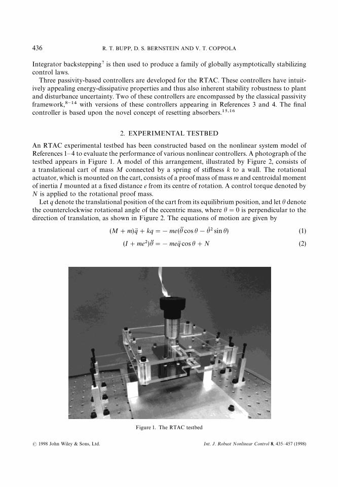
An RTAC experimental testbed has been constructed based on the nonlinear system model ofReferences 1—4 to evaluate the performance of various nonlinear controllers. A photograph of thetestbed appears in Figure 1. A model of this arrangement, illustrated by Figure 2, consists ofa translational cart of mass M connected by a spring of stiffness k to a wall. The rotationalactuator, which is mounted on the cart, consists of a proof mass of mass m and centroidal momentof inertia I mounted at a fixed distance e from its centre of rotation. A control torque denoted byN is applied to the rotational proof mass.

Let q denote the translational position of the cart from its equilibrium position, and let h denotethe counterclockwise rotational angle of the eccentric mass, where h"0 is perpendicular to thedirection of translation, as shown in Figure 2. The equations of motion are given by

(M#m)q(#kq"!me(h$ cos h!hQ 2 sin h) (1)

(I#me2)h$"!meq( cos h#N (2)

Figure 1. The RTAC testbed

436 R. T. BUPP, D. S. BERNSTEIN AND V. T. COPPOLA

( 1998 John Wiley & Sons, Ltd. Int. J. Robust Nonlinear Control 8, 435—457 (1998)

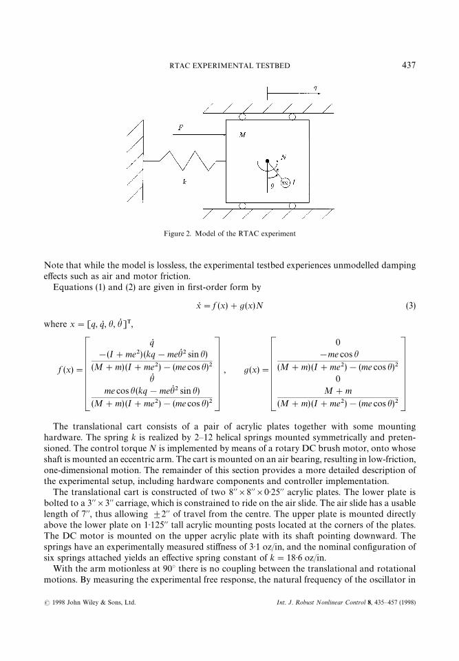
Figure 2. Model of the RTAC experiment

Note that while the model is lossless, the experimental testbed experiences unmodelled dampingeffects such as air and motor friction.

Equations (1) and (2) are given in first-order form by

xR "f (x)#g(x)N (3)

where x"[q, qR , h, hQ ]T,

f (x)"

qR!(I#me2) (kq!mehQ 2 sin h)

(M#m) (I#me2)!(me cos h)2hQ

me cos h(kq!mehQ 2 sin h)

(M#m) (I#me2)!(me cos h)2

, g(x)"

0!me cos h


M#m


The translational cart consists of a pair of acrylic plates together with some mountinghardware. The spring k is realized by 2—12 helical springs mounted symmetrically and preten-sioned. The control torque N is implemented by means of a rotary DC brush motor, onto whoseshaft is mounted an eccentric arm. The cart is mounted on an air bearing, resulting in low-friction,one-dimensional motion. The remainder of this section provides a more detailed description ofthe experimental setup, including hardware components and controller implementation.

The translational cart is constructed of two 8@@]8@@]0)25@@ acrylic plates. The lower plate isbolted to a 3@@]3@@ carriage, which is constrained to ride on the air slide. The air slide has a usablelength of 7@@, thus allowing $2@@ of travel from the centre. The upper plate is mounted directlyabove the lower plate on 1)125@@ tall acrylic mounting posts located at the corners of the plates.The DC motor is mounted on the upper acrylic plate with its shaft pointing downward. Thesprings have an experimentally measured stiffness of 3)1 oz/in, and the nominal configuration ofsix springs attached yields an effective spring constant of k"18)6 oz/in.

With the arm motionless at 90° there is no coupling between the translational and rotationalmotions. By measuring the experimental free response, the natural frequency of the oscillator in

437RTAC EXPERIMENTAL TESTBED


this configuration was determined to be 1)64 Hz. Since the way in which the experiment wasconstructed made it difficult to determine the mass of each subpart precisely, the measuredstiffness and the measured natural frequency were used to identify the effective mass of the cart.This total mass M consisting of the masses of the acrylic plates, the mounting section of the airslide, the DC motor, and the mounting hardware was determined to be approximately 65 oz. Thedamping ratio of the oscillator with the eccentric arm held motionless was also determined fromthe free response characteristics and was seen to vary from approximately 0)45% when the RTACis configured for experimentation, to less than 0)1% when no power or data cables are attached.The supply hose for the air slide must remain attached to the cart, however, and the air dragresulting from the motion of the hose and the cart is responsible for much of the remainingdamping.

The eccentric arm connected to the motor shaft is a 4)25@@]0)75@@]0)0625@@ aluminium bar, intowhich a 2)75@@ long slot is cut to facilitate mounting additional proof masses. The bar is attachedto a steel collar which is fastened with set screws to the shaft of the DC motor. While the eccentricarm alone serves as a rotational proof mass, additional proof masses constructed of steel can bemounted to the eccentric arm at a range of locations. The additional proof masses are each0)75@@]0)75@@]0)0625@@ and weigh 0)14 oz. They can be stacked as many as six high, and mountedon the arm between 1)5@@ and 3)25@@ from the motor shaft. The aluminium arm is scored at 0)125@@intervals to permit repeatability of the experimental configuration when additional proof massesare attached. The effective values of the parameters m, e, and I vary depending on the number andlocation of the attached proof masses. With no proof masses attached to the arm, m"1)56 oz,e"1)76@@ and I"0)74 oz in2, where m is measured, and e and I are calculated based on geometryand material properties. When no additional proof masses are attached to the arm, the valueof the coupling parameter e, which will be defined in Section 3, is e"0)14. In a typicalconfiguration of 5 additional proof masses mounted on the arm 3)875@@ from the rotation axis, thecoupling increases to e"0)18. The physical parameters of the RTAC testbed are summarized inTable I.

The torque actuation is provided by a 12 V DC brush motor which is 2)25@@ long and 1)38@@ indiameter. The motor produces 3)04 oz in/A, and is rated for continuous torque of 14)2 oz in, andcontinuous power output of 45 W. To achieve the torque ratings, the motor is capable ofoperating with a continuous 4)67 A load, although higher currents can be tolerated for shortperiods of time. In order to utilize torque as the control input, we use a DC servo drive tocommand the current into the motor. The pulse-width-modulated drive is rated to produce 5 Acontinuous current and 10 A peak current with a bandwidth of 2)5 kHz.

Table I. Summary of the RTAC physical parameters

Bare arm 5 Added proofmasses

Cart mass M 65)5 oz 65)5 ozArm mass m 1)56 oz 2)28 ozSpring constant k 18)6 oz/in 18)6 oz/inEccentricity e 1)76 in 2)43 inArm inertia I 0)74 oz in2 0)74 oz inCoupling e 0)14 0)18



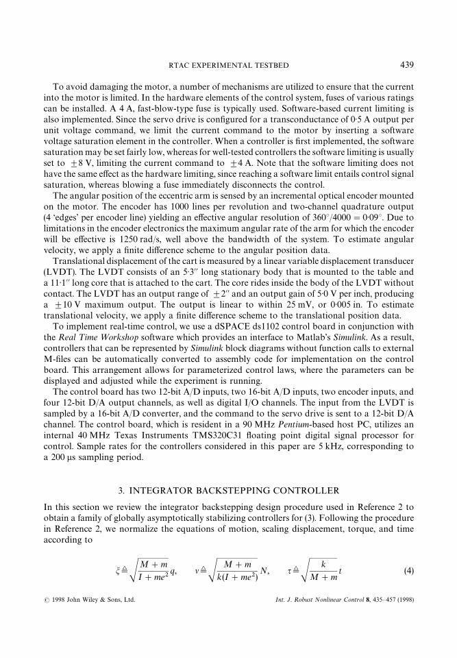
To avoid damaging the motor, a number of mechanisms are utilized to ensure that the currentinto the motor is limited. In the hardware elements of the control system, fuses of various ratingscan be installed. A 4 A, fast-blow-type fuse is typically used. Software-based current limiting isalso implemented. Since the servo drive is configured for a transconductance of 0)5 A output perunit voltage command, we limit the current command to the motor by inserting a softwarevoltage saturation element in the controller. When a controller is first implemented, the softwaresaturation may be set fairly low, whereas for well-tested controllers the software limiting is usuallyset to $8 V, limiting the current command to $4 A. Note that the software limiting does nothave the same effect as the hardware limiting, since reaching a software limit entails control signalsaturation, whereas blowing a fuse immediately disconnects the control.

The angular position of the eccentric arm is sensed by an incremental optical encoder mountedon the motor. The encoder has 1000 lines per revolution and two-channel quadrature output(4 ‘edges’ per encoder line) yielding an effective angular resolution of 360°/4000"0)09°. Due tolimitations in the encoder electronics the maximum angular rate of the arm for which the encoderwill be effective is 1250 rad/s, well above the bandwidth of the system. To estimate angularvelocity, we apply a finite difference scheme to the angular position data.

Translational displacement of the cart is measured by a linear variable displacement transducer(LVDT). The LVDT consists of an 5)3@@ long stationary body that is mounted to the table anda 11)1@@ long core that is attached to the cart. The core rides inside the body of the LVDT withoutcontact. The LVDT has an output range of $2@@ and an output gain of 5)0 V per inch, producinga $10 V maximum output. The output is linear to within 25 mV, or 0)005 in. To estimatetranslational velocity, we apply a finite difference scheme to the translational position data.

To implement real-time control, we use a dSPACE ds1102 control board in conjunction withthe Real ¹ime ¼orkshop software which provides an interface to Matlab’s Simulink. As a result,controllers that can be represented by Simulink block diagrams without function calls to externalM-files can be automatically converted to assembly code for implementation on the controlboard. This arrangement allows for parameterized control laws, where the parameters can bedisplayed and adjusted while the experiment is running.

The control board has two 12-bit A/D inputs, two 16-bit A/D inputs, two encoder inputs, andfour 12-bit D/A output channels, as well as digital I/O channels. The input from the LVDT issampled by a 16-bit A/D converter, and the command to the servo drive is sent to a 12-bit D/Achannel. The control board, which is resident in a 90 MHz Pentium-based host PC, utilizes aninternal 40 MHz Texas Instruments TMS320C31 floating point digital signal processor forcontrol. Sample rates for the controllers considered in this paper are 5 kHz, corresponding toa 200 ls sampling period.

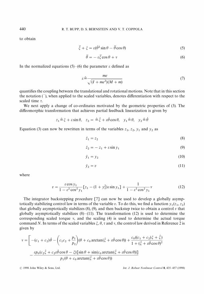
3. INTEGRATOR BACKSTEPPING CONTROLLER

In this section we review the integrator backstepping design procedure used in Reference 2 toobtain a family of globally asymptotically stabilizing controllers for (3). Following the procedurein Reference 2, we normalize the equations of motion, scaling displacement, torque, and timeaccording to

m¢SM#m

I#me2q, l¢S

M#m

k(I#me2)N, q¢S

k

M#mt (4)



to obtain

m$#m"e(hQ 2 sin h!h$ cos h) (5)

h$"!em$ cos h#l (6)

In the normalized equations (5)— (6) the parameter e defined as

e¢me

J(I#me2) (M#m)(7)

quantifies the coupling between the translational and rotational motions. Note that in this sectionthe notation ( ) ), when applied to the scaled variables, denotes differentiation with respect to thescaled time q.

We next apply a change of co-ordinates motivated by the geometric properties of (3). Thediffeomorphic transformation that achieves partial feedback linearization is given by

z1¢m#e sin h, z

2"¢mQ #ehQ cos h, y

1¢h, y

2¢hQ

Equation (3) can now be rewritten in terms of the variables z1, z

2, y

1and y

2as

zR1"z

2(8)

zR2"!z

1#e sin y

1(9)

yR1"y

2(10)

yR2"v (11)

where

v"e cos y

11!e2 cos2 y

1

[z1!(1#y2

2)e sin y

1]#

1

1!e2 cos2 y1

l (12)

The integrator backstepping procedure [7] can now be used to develop a globally asymp-totically stabilizing control law in terms of the variable v. To do this, we find a function y

1(z

1, z

2)

that globally asymptotically stabilizes (8), (9), and then backstep twice to obtain a control v thatglobally asymptotically stabilizes (8)— (11). The transformation (12) is used to determine thecorresponding scaled torque l, and the scaling (4) is used to determine the actual torquecommand N. In terms of the scaled variables m, h, q and l, the control law derived in Reference 2 isgiven by

l"C!(c1#c

2)hQ !Ac1c2#

p1

p2B (h#c

0arctan(mQ #ehQ cos h))#

c0((c

1#c

2)m#mQ )

1#(mQ #ehQ cos h)2

!

ep0(c

2mQ #c

2ehQ cos h!m) [sin h#sin(c

0arctan(mQ #ehQ cos h))]

p1(h#c

0arctan(mQ #ehQ cos h ))



#2c0m2(mQ #ehQ cos h)

(1#(mQ #ehQ cos h)2)2#

ep0c0m(mQ #ehQ cos h)cos(c

0arctan(mQ #ehQ cos h))

p1(1#(mQ #ehQ cos h)2) (h#c


!

ep0(mQ #ehQ cos h)hQ cos h

p1(h#c


#

ep0hQ (mQ #ehQ cos h) [sin h#sin(c

0arctan(mQ #ehQ cos h))]

p1(h#c

0arctan(mQ #ehQ cos h))2

!

e cos h1!e2 cos2 h

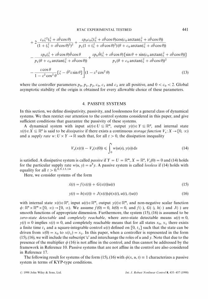
[m!hQ 2e sin h]D (1!e2 cos2 h) (13)

where the controller parameters p0, p

1, p

2, c

0, c

1and c

2are all positive, and 0(c

0(2. Global

asymptotic stability of the origin is obtained for every allowable choice of these parameters.

4. PASSIVE SYSTEMS

In this section, we define dissipativity, passivity, and losslessness for a general class of dynamicalsystems. We then restrict our attention to the control systems considered in this paper, and givesufficient conditions that guarantee the passivity of these systems.

A dynamical system with input u(t)3º-Rm, output y (t)3½-Rp, and internal statex(t)3X-Rn is said to be dissipative if there exists a continuous storage function »

s: XP[0,R)

and a supply rate w :º]½PR such that, for all t'0, the dissipation inequality

»s(x(t))!»

s(x(0)))P

t

0

w (u(s), y (s)) ds (14)

is satisfied. A dissipative system is called passive if ½"º"Rm, X"Rn, »s(0)"0 and (14) holds

for the particular supply rate w (u, y)"uTy. A passive system is called lossless if (14) holds withequality for all t'0.8,9,13,14

Here, we consider systems of the form

xR (t)"f (x(t))#G(x (t))u (t) (15)

y(t)"h (x(t))#J (x(t))/ (x(t), u(t), t)u(t) (16)

with internal state x (t)3Rn, input u (t)3Rm, output y (t)3Rm, and non-negative scalar function/ :Rn]Rm][0,R)P[0,R). We assume f (0)"0, h (0)"0, and f ( ) ), G( ) ), h ( ) ) and J ( ) ) aresmooth functions of appropriate dimension. Furthermore, the system (15), (16) is assumed to bezero-state detectable and completely reachable, where zero-state detectable means u(t),0,y(t),0 implies x(t),0, and completely reachable means that for all states x

0, x

1there exists

a finite time t1

and a square-integrable control u (t) defined on [0, t1] such that the state can be

driven from x (0)"x0

to x (t1)"x

1. In this paper, when a controller is represented in the form

(15), (16), we will include the subscript ‘c’ and interchange the roles of u and y. Note that due to thepresence of the multiplier / (16) is not affine in the control, and thus cannot be addressed by theframework in Reference 10. Passive systems that are not affine in the control are also consideredin Reference 17.

The following result for systems of the form (15), (16) with /(x, u, t),1 characterizes a passivesystem in terms of KYP-type conditions.



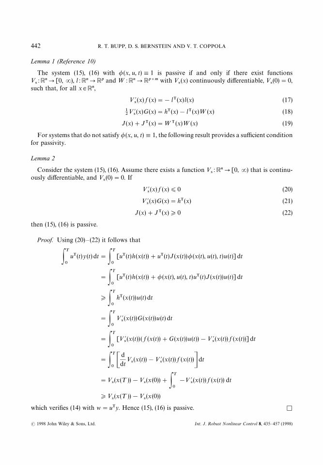
Lemma 1 (Reference 10)

The system (15), (16) with /(x, u, t),1 is passive if and only if there exist functions»

4:RnP[0,R), l :RnPRp and ¼ :RnPRp]m with »

4(x) continuously differentiable, »

4(0)"0,

such that, for all x3Rn,

» @4(x) f (x)"!lT (x)l(x) (17)

12» @

4(x)G(x)"hT (x)!lT (x)¼ (x) (18)

J(x)#JT(x)"¼T (x)¼(x) (19)

For systems that do not satisfy / (x, u, t),1, the following result provides a sufficient conditionfor passivity.

Lemma 2

Consider the system (15), (16). Assume there exists a function »4: RnP[0,R) that is continu-

ously differentiable, and »4(0)"0. If

» @4(x) f (x))0 (20)

» @4(x)G(x)"hT (x) (21)

J(x)#JT(x)*0 (22)

then (15), (16) is passive.

Proof. Using (20)— (22) it follows that

PT

0

uT(t)y (t) dt"PT

0

[uT(t)h (x(t))#uT(t)J (x(t))/ (x(t), u(t), t)u (t)] dt

"PT

0

[uT(t)h (x(t))#/ (x(t), u(t), t)uT (t)J (x (t))u (t)] dt

*PT

0

hT(x (t))u (t) dt

"PT

0

» @4(x (t))G(x (t))u (t) dt

"PT

0

[» @4(x (t)) ( f (x(t))#G(x(t))u(t))!» @

4(x (t)) f (x (t))] dt

"PT

0C

d

dt»

4(x(t))!» @

4(x (t)) f (x (t))Ddt

"»4(x(¹ ))!»

4(x (0))#P

T

0

!» @4(x(t)) f (x(t)) dt

*»4(x(¹ ))!»

4(x (0))

which verifies (14) with w"uTy. Hence (15), (16) is passive. K



Two well-known properties of passive systems will be exploited in this paper: passive systemsare stable in the sense of Lyapunov, and the negative feedback interconnection of two passivesystems is passive with respect to the inputs and outputs of either of the original systems, and thusis Lyapunov stable.11,12

5. PASSIVE CONTROLLERS

Our primary objective for controller design is to asymptotically stabilize the origin x"0 of thesystem (3). In order to exploit the stability robustness property associated with the feedbackconnection of a passive plant with a passive controller, we must first ensure that the plant to becontrolled is passive. However, due to the rigid-body rotational mode, the undamped RTACmodel (3) is actually unstable, and, accordingly, not passive. Therefore, the approach we take forcontrol design is to passify the plant model using bounded state feedback, and then investigate theperformance of various asymptotically stabilizing passive control designs.

Note that our stability objective, namely, asymptotic stability of the origin, necessarilyredefines the equilibrium structure of the system, since the equilibria of the open-loop system havethe form q"0, qR "0 and hQ "0, with h arbitrary. In our passive controller designs, we include thecondition that the controller should not distinguish between the states h mod 2n, since theinability of the controller to recognize this physical equivalence can result in undesirableunwinding behaviour.3 An example of unwinding is given in Section 6.2.

5.1. Passifying the plant model

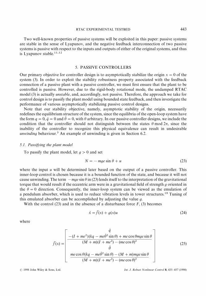
To passify the plant model, let g'0 and set

N"!mge sin h#u (23)

where the input u will be determined later based on the output of a passive controller. Thisinner-loop control is chosen because it is a bounded function of the state, and because it will notcause unwinding. The term !mge sin h in (23) lends itself to the interpretation of the gravitationaltorque that would result if the eccentric arm were in a gravitational field of strength g oriented inthe h"0 direction. Consequently, the inner-loop system can be viewed as the emulation ofa pendulum absorber, which is used to reduce vibration levels in tower structures.18 Tuning ofthis emulated absorber can be accomplished by adjusting the value g.

With the control (23) and in the absence of a disturbance force F, (3) becomes

xR "fM (x)#g(x)u (24)

where

fM (x)"

qR!(I#me2) (kq!mehQ 2 sin h)#me cos hmge sin h


hQme cos h(kq!mehQ 2 sin h)!(M#m)mge sin h


(25)



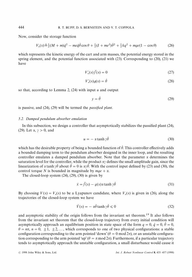
Now, consider the storage function

»4(x)¢1

2(M#m)qR 2!meqR hQ cos h#1

2(I#me2)hQ 2#1

2kq2#mge(1!cos h) (26)

which represents the kinetic energy of the cart and arm masses, the potential energy stored in thespring element, and the potential function associated with (23). Corresponding to (20), (21) wehave

» @4(x) fM (x)"0 (27)

» @4(x)g(x)"hQ (28)

so that, according to Lemma 2, (24) with input u and output

y"hQ (29)

is passive, and (24), (29) will be termed the passified plant.

5.2. Damped pendulum absorber emulation

In this subsection, we design a controller that asymptotically stabilizes the passified plant (24),(29). Let a, c'0, and

u"!a tanh chQ (30)

which has the desirable property of being a bounded function of hQ . This controller effectively addsa bounded damping term to the pendulum absorber designed in the inner loop, and the resultingcontroller emulates a damped pendulum absorber. Note that the parameter a determines thesaturation level for the controller, while the product ac defines the small amplitude gain, since thelinearization of a tanh chQ about hQ "0 is achQ . With the control input defined by (23) and (30), thecontrol torque N is bounded in magnitude by mge#a.

The closed-loop system (24), (29), (30) is given by

xR "fM (x)!g (x)a tanh chQ (31)

By choosing » (x)"»4(x) to be a Lyapunov candidate, where »

4(x) is given in (26), along the

trajectories of the closed-loop system we have

»Q (x)"!ahQ tanh chQ )0 (32)

and asymptotic stability of the origin follows from the invariant set theorem.19 It also followsfrom the invariant set theorem that the closed-loop trajectory from every initial condition willasymptotically approach an equilibrium position in state space of the form q"0, qR "0, hQ "0,h"nn, n"0, $1, $2,2, which corresponds to one of two physical configurations: a stableconfiguration corresponding to the arm pointed ‘down’ (h"0 mod2n), or an unstable configura-tion corresponding to the arm pointed ‘up’ (h"nmod 2n). Furthermore, if a particular trajectorytends to asymptotically approach the unstable configuration, a small disturbance would cause it



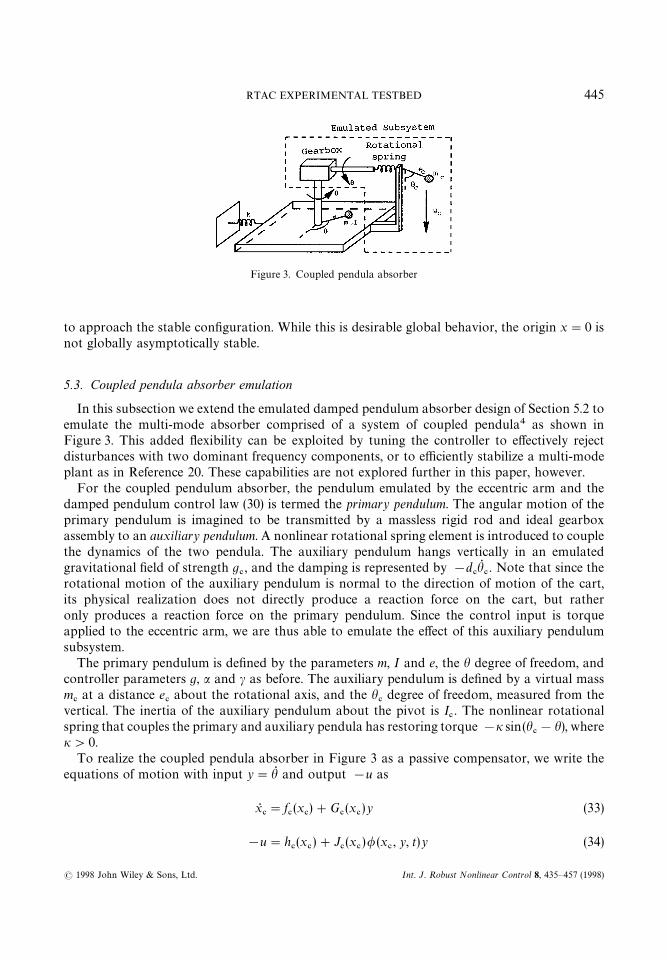
Figure 3. Coupled pendula absorber

to approach the stable configuration. While this is desirable global behavior, the origin x"0 isnot globally asymptotically stable.

5.3. Coupled pendula absorber emulation

In this subsection we extend the emulated damped pendulum absorber design of Section 5.2 toemulate the multi-mode absorber comprised of a system of coupled pendula4 as shown inFigure 3. This added flexibility can be exploited by tuning the controller to effectively rejectdisturbances with two dominant frequency components, or to efficiently stabilize a multi-modeplant as in Reference 20. These capabilities are not explored further in this paper, however.

For the coupled pendulum absorber, the pendulum emulated by the eccentric arm and thedamped pendulum control law (30) is termed the primary pendulum. The angular motion of theprimary pendulum is imagined to be transmitted by a massless rigid rod and ideal gearboxassembly to an auxiliary pendulum. A nonlinear rotational spring element is introduced to couplethe dynamics of the two pendula. The auxiliary pendulum hangs vertically in an emulatedgravitational field of strength g

#, and the damping is represented by !d

#hQ#. Note that since the

rotational motion of the auxiliary pendulum is normal to the direction of motion of the cart,its physical realization does not directly produce a reaction force on the cart, but ratheronly produces a reaction force on the primary pendulum. Since the control input is torqueapplied to the eccentric arm, we are thus able to emulate the effect of this auxiliary pendulumsubsystem.

The primary pendulum is defined by the parameters m, I and e, the h degree of freedom, andcontroller parameters g, a and c as before. The auxiliary pendulum is defined by a virtual massm

#at a distance e

#about the rotational axis, and the h

#degree of freedom, measured from the

vertical. The inertia of the auxiliary pendulum about the pivot is I#. The nonlinear rotational

spring that couples the primary and auxiliary pendula has restoring torque !i sin(h#!h), where

i'0.To realize the coupled pendula absorber in Figure 3 as a passive compensator, we write the

equations of motion with input y"hQ and output !u as

xR#"f

#(x

#)#G

#(x

#)y (33)

!u"h#(x

#)#J

#(x

#)/ (x

#, y, t)y (34)



where x#"[h h

#hQ#]T, and

f#(x

#)"

0

hQ#

!

i sin(h#!h)

I#

!

m#g#e#sin h

#I#

!

d#

I#

hQ#

, G#(x

#)"

1

0

0

(35)

h#(x

#)"i sin(h!h

#), J

#(x

#)"a, / (x

#, y, t)"

tanh cyy

(36)

Notice that since 0(/ (y)(1, (33), (34) is of the form (15), (16).A storage function for the compensator (33)— (36) is given by

»4#

(x#)¢1

2I#hQ 2##m

#g#e#(1!cos h

#)#i (1!cos(h!h

#)) (37)

which represents the kinetic energy of the auxiliary pendulum plus the potential energies of theauxiliary pendulum and the elastic coupling. The system (33)— (36) with input y, output !u, andstorage function »

4#(x

#) satisfies

» @4#

(x#) f

#(x

#)"0 (38)

» @4#

(x#)G

#(x

#)"hT

#(x

#) (39)

J#(x

#)#JT

#(x

#)"2a'0 (40)

corresponding to the conditions of Lemma 2. The compensator is thus passive.Because the closed-loop system is comprised of the negative feedback interconnection of

passive systems, it is passive, and thus Lyapunov stable. Asymptotic stability of the closed-loopsystem follows from the invariant set theorem, where »

#-(x, x

#)"»

4(x)#»

4#(x

#) is used as

a Lyapunov function for the closed-loop system. It also follows from the invariant set theoremthat the stability properties of the equilibria q"0, qR "0, hQ "0, hQ

#"0, h"$n

1n, h

#"$n

2n for

integers n1

and n2, are qualitatively similar to those of the closed-loop system involving the

damped pendulum absorber of Section 5.2 in that all closed-loop trajectories asymptoticallyapproach the origin, modulo n in the rotational states h, h

#.

5.4. Virtual resetting absorber controllers

The third dissipative controller we consider is a virtual resetting absorber controller, whichemulates an absorber system whose states are reset to achieve instantaneous reduction of the‘total energy’ of the closed-loop system, where the total energy includes the kinetic and potentialenergies associated with the actual physical plant, as well as the emulated energy associated withthe states of the controller. One type of virtual resetting controller, called a virtual trap-doorabsorber, is described in Reference 15, where the resetting algorithm is used to achieve finite-timestabilization of the double integrator. A general theory of virtual resetting absorber controllers isdeveloped in Reference 16. Resetting differential systems are also considered in References 21 and22 as a special case of differential equations with impulse effect.



Resetting differential systems consist of three main elements: a continuous-time dynamicalequation, which governs the motion of the system between resetting events; a difference equation,which governs the way the states of the controller are instantaneously changed when a resettingevent occurs; and a condition that determines when the states of the system are to be reset. Theevolution of the state of a resetting differential system is as follows: while the resetting condition isnot met, the state is given by the solution of the differential equation, with appropriate initialconditions. Upon reaching a point in time and/or state space that satisfies the resetting condition,the state of the system is instantaneously reset according to the resetting law. The state thenproceeds to evolve as a solution of the differential equation again, until the resetting condition isagain satisfied.

The resetting controller is given by

xR#"C

hQ#

!iI#

sin(h#!h)D, ihQ sin(h!h

#)'0 (41)

*x#"C

h!h#

!hQ#D, ihQ sin(h!h

#))0 (42)

u"i sin(h#!h) (43)

The continuous-time equation governing the behavior of the state x#between resetting events is

given by (41). These dynamics represent the coupled pendula absorber of Section 5.3 where thegravity term g

#and the dissipation term d

#are both set to zero. Notice that unlike the passive

controller designs of Sections 5.2 and 5.3, this controller has no dissipation term in its dynamics(41).

The resetting law (42) describes the instantaneous change in the controller state that occurswhen the resetting condition is met; that is, when the resetting condition is met, the state x

#is

instantly reset to x##*x

#, and thus, according to (42), h

#is reset to h

##h!h

#"h, and h

#is

reset to hQ#!hQ

#"0. This resetting law (42) thus resets h

#to h and hQ

#to 0.

The resetting condition in (41), (42) involves a sign condition on the function ihQ sin(h!h#). The

motivation for this condition, as well as for the form of the reset law (42), is based on properties ofthe emulated energy, which is given by

»#(x

#, x)"1

2I#hQ 2##i (1!cos(h!h

#))*0 (44)

When the resetting condition is not met, it follows from (41) that

d

dt»

#(x

#, x)"ihQ sin(h!h

#) (45)

It follows from (24)— (28) and (41)— (45) that

d

dt»

#(x

#, x)"ihQ sin(h!h

#)"!hQ u"!

d

dt»

4(x) (46)

Thus, »#is increasing if and only if »

4is decreasing. It is now clear from (41), (42) and (45) that the

resetting condition (42) allows the states of the controller to evolve without resetting as long as



the emulated energy (44) is increasing; that is, no resetting occurs provided the controller isremoving energy from the plant (24). When the controller is no longer able to remove energy fromthe RTAC, the controller states are reset with h

#reset to h, and hQ

#reset to 0. This change in

controller state causes the emulated energy (44) to be instantly transferred from »#(x

#, x)*0 to

»#(x

##*x

#, x)"0, effectively dumping any ‘energy’ that had accumulated in the controller.

In this approach, energy is allowed to flow from the plant into the controller, but due to theresetting mechanism, no energy can flow from the controller back to the plant. Hence, in thediscussion that follows, we will refer to this resetting controller as the virtual one-way absorber, orsimply the one-way absorber. While this resetting algorithm has no mechanism for doing positivework on the plant, its discrete resetting action (42) prevents it from being captured by thestandard dissipativity framework.

To implement the one-way absorber controller on the RTAC, only the angle h is measured. Thevalue of the compensator energy (44) is evaluated at each time step, and the controller states arereset whenever the compensator energy is less than or equal to the value of the compensatorenergy at the previous sampling instant.

6. EXPERIMENTAL RESULTS

6.1. Performance comparison

In this section, the controller designs of Sections 3 and 5 are implemented and evaluated on theRTAC testbed. The baseline experiment used to evaluate the performance of the controllers is aninitial condition response, where q(0)"1)5@@ and qR (0)"0. This initial condition is roughly aslarge as the testbed will allow, and the responses are representative of those obtained at otherinitial conditions. For the passivity-based controllers, the arm is set initially to h"0 and hQ (0)"0.With the RTAC held in this initial configuration, the controller is active, although no controltorque is applied by the motor. The experiment begins when the cart is released. For theintegrator backstepping controller, when the cart is held motionless at q (0)"1)5@@, controltorques cause the arm to be initially at rest at approximately h"145°.

The time histories of the cart position and arm angle are recorded, and the value of the controlsignal is computed by multiplying the output of the controller (measured in volts) times thetransconductance of the servo drive (0)53 A/V) times the motor constant (3)04 oz in/A). For eachexperiment, a settling time is computed as the time required for the cart displacement to becomeless than 10% of the initial value, that is, 0)15@@. An approximate damping ratio is assigned to eachresponse based on logarithmic decrement analysis. Clearly, the responses of these nonlinearsystems are not expected to mimic the response of a linear system. However, by approximatingthe rate of decrease of the amplitude of the cart displacement during roughly the first 5 s of theexperiment, an effective damping ratio can be assigned that is useful for comparison purposes.A summary of the performance of the various controllers is given in Table II.

The open-loop response to the given initial condition is given in Figure 4. Note that in theabsence of control, the eccentric arm tends to drift into a position parallel with the axis oftranslation. In this case, the arm tends toward !90°.

The integrator backstepping controller described in Section 3 is implemented with p0"5000,

p1"500, p

2"500, c

0"0)5, c

1"1 and c

2"1. These parameters were selected by trial and error

as it is not clear precisely what role is played by the individual controller parameters indetermining the closed-loop response. The strategy is to choose controller parameters that



Table II. Summary of controller performance

Controller f!11309

u.!9

Open loop 0)44% —Coupled pendula absorber 3)2% 0)52 oz inIntegrator backstepping 3)7% 12)2 oz in

(saturated)Damped pendulum absorber 5)1% 0)47 oz inVirtual resetting absorber 5)2% 0)44 oz in

Figure 4. Uncontrolled response of the RTAC to a 1)5 in initial displacement

minimize the settling time from the given baseline initial condition. The factor most responsiblefor limiting the performance of this controller is the maximum current constraint. The currentlimiter is set to 4 A or 12)2 oz in of torque.

The experimental initial-condition response is shown in Figure 5. The initial angle of the arm isabout 145°, which is due to the control torques generated by the full-state feedback controllerwhen the cart is held at q"1)5@@. The integrator backstepping controller settles the cart to 10% ofthe initial displacement in about 6 s. Based on logarithmic decrement analysis during this period,the effective damping ratio is approximately 3)7%. The controller then continues to bring the cartand arm to rest at the desired zero position. The controller output is characterized by a largeamplitude control signal—saturating often during the initial two seconds—with substantial high



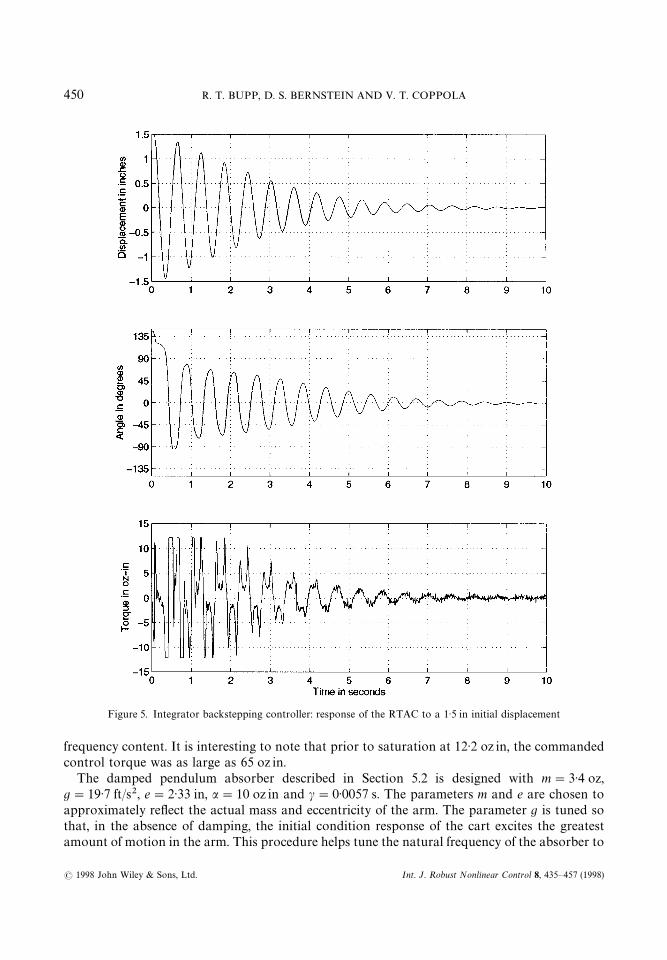
Figure 5. Integrator backstepping controller: response of the RTAC to a 1)5 in initial displacement

frequency content. It is interesting to note that prior to saturation at 12)2 oz in, the commandedcontrol torque was as large as 65 oz in.

The damped pendulum absorber described in Section 5.2 is designed with m"3)4 oz,g"19)7 ft/s2, e"2)33 in, a"10 oz in and c"0)0057 s. The parameters m and e are chosen toapproximately reflect the actual mass and eccentricity of the arm. The parameter g is tuned sothat, in the absence of damping, the initial condition response of the cart excites the greatestamount of motion in the arm. This procedure helps tune the natural frequency of the absorber to



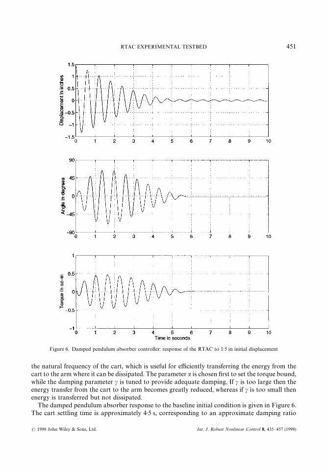
Figure 6. Damped pendulum absorber controller: response of the RTAC to 1)5 in initial displacement

the natural frequency of the cart, which is useful for efficiently transferring the energy from thecart to the arm where it can be dissipated. The parameter a is chosen first to set the torque bound,while the damping parameter c is tuned to provide adequate damping. If c is too large then theenergy transfer from the cart to the arm becomes greatly reduced, whereas if c is too small thenenergy is transferred but not dissipated.

The damped pendulum absorber response to the baseline initial condition is given in Figure 6.The cart settling time is approximately 4)5 s, corresponding to an approximate damping ratio



of 5)1%. After this time, the cart suffers residual oscillations of approximately 0)04@@ amplitudethat are not damped by the controller. The control signal appears smooth.

The coupled pendula absorber described in Section 5.3 is designed with m"3)4 oz,g"34)6 ft/s2, e"2)33 in, a"10 oz in, c"0)0057 s, i"14)2 oz in, I

#"11)3 oz in2, e

#"0, and

d#"14)2 oz in sec. Here again the parameters m and e are chosen to reflect the actual mass and

eccentricity of the arm. The design of the remaining parameters is more complicated than thedesign of the damped pendulum absorber since the absorber subsystem here is of higher order. Toachieve good settling behaviour, the parameters are tuned so that the initial condition response ofthe cart excites one ‘mode’ of the coupled pendulum absorber system as much as possible. Theother ‘mode’ of the absorber could in theory be tuned to achieve improved disturbance rejectionfor disturbances at some other frequency, or to improve settling behaviour of some other mode ofthe plant.

The coupled pendula absorber response to the baseline initial condition is given in Figure 7.The cart settling time is approximately 6)75 s, corresponding to an approximate damping ratio of3)2%, based on logarithmic decrement analysis during the 5)5 s of the experiment. The cart suffersresidual oscillations of approximately 0)1@@ amplitude that are not damped by the controller. Thecontrol signal appears smooth and appears to possess two dominant frequencies components.

The one-way absorber controller described in Section 5.4 is designed with m"3)4 oz,g"19)7 ft/s2, e"2)33 in, i"4)25 oz in and I

#"1)1 oz in2. As was the case for the previous

absorber-based controllers, the parameters m and e are chosen to reflect the actual mass andeccentricity of the arm. As it was for the damped pendulum absorber controller, the parameter g ischosen to allow the most efficient energy transfer from the cart to the eccentric arm. Now, insteadof proceeding to the selection of the proper dashpot parameter as we did in the damped pendulumabsorber design, we simply design the controller parameters i and I

#to exchange energy

efficiently with the eccentric arm. Since the one-way controller is implemented on a digital controlboard with a 200 ls sampling period, a comparison of the current value of the emulated energy(44) with the value of the emulated energy computed during the previous sample interval is usedto determine whether or not the controller emulated energy has stopped increasing. When theemulated energy has stopped increasing, the states of the controller are reset so that the value ofthe controller energy function is zero.

The response of the one-way absorber controller to the baseline initial condition is given inFigure 8. The settling time for this controller is approximately 4)5 s which corresponds to anapproximate damping ratio of 5)2%. Residual cart oscillations of 0)08@@ amplitude are not dampedby the controller. Some discontinuity in the control signal due to the resetting nature of thiscontroller is apparent in the figure.

One major difference between the integrator backstepping controller and the passive designscan be seen in the cart displacement response as time progresses. It has been noted in all of thepassivity-based control cases that there is a residual oscillation of the cart that the controllerscannot remove. This is due to the stiction in the motor/arm assembly which is not included in thedynamical model and which causes the zero-state detectability condition to fail. For oscillationsof this level, the accelerations of the cart are so small that the stiction force alone keeps thearm from moving, and, without motion in the arm, energy cannot be removed from the cart.To contrast, the integrator backstepping controller, being a full-state-feedback controllaw, applies torque based on measured cart displacement and velocity, and thus, despite thepresence of stiction, can remove the low-amplitude cart oscillations that the passive controllerscannot.



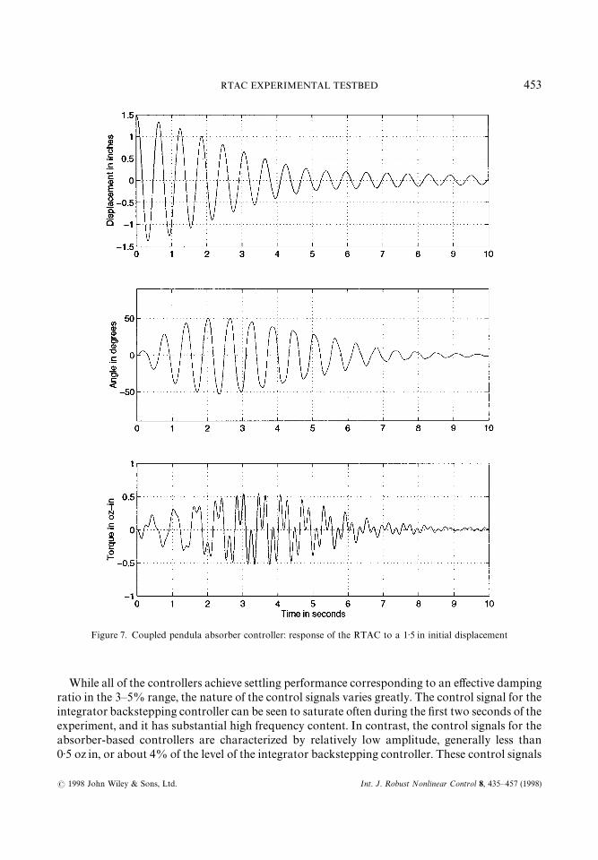
Figure 7. Coupled pendula absorber controller: response of the RTAC to a 1)5 in initial displacement

While all of the controllers achieve settling performance corresponding to an effective dampingratio in the 3—5% range, the nature of the control signals varies greatly. The control signal for theintegrator backstepping controller can be seen to saturate often during the first two seconds of theexperiment, and it has substantial high frequency content. In contrast, the control signals for theabsorber-based controllers are characterized by relatively low amplitude, generally less than0)5 oz in, or about 4% of the level of the integrator backstepping controller. These control signals



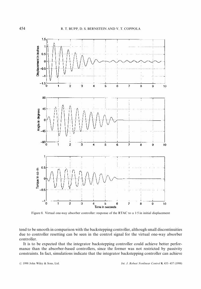
Figure 8. Virtual one-way absorber controller: response of the RTAC to a 1)5 in initial displacement

tend to be smooth in comparison with the backstepping controller, although small discontinuitiesdue to controller resetting can be seen in the control signal for the virtual one-way absorbercontroller.

It is to be expected that the integrator backstepping controller could achieve better perfor-mance than the absorber-based controllers, since the former was not restricted by passivityconstraints. In fact, simulations indicate that the integrator backstepping controller can achieve



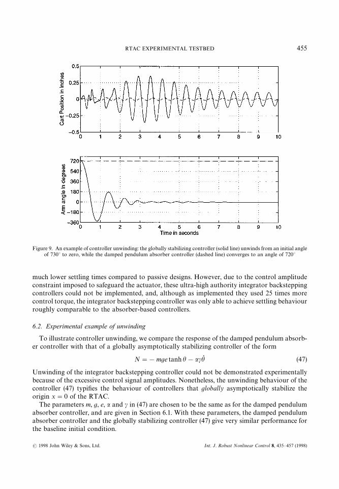
Figure 9. An example of controller unwinding: the globally stabilizing controller (solid line) unwinds from an initial angleof 730° to zero, while the damped pendulum absorber controller (dashed line) converges to an angle of 720°

much lower settling times compared to passive designs. However, due to the control amplitudeconstraint imposed to safeguard the actuator, these ultra-high authority integrator backsteppingcontrollers could not be implemented, and, although as implemented they used 25 times morecontrol torque, the integrator backstepping controller was only able to achieve settling behaviourroughly comparable to the absorber-based controllers.

6.2. Experimental example of unwinding

To illustrate controller unwinding, we compare the response of the damped pendulum absorb-er controller with that of a globally asymptotically stabilizing controller of the form

N"!mge tanh h!achQ (47)

Unwinding of the integrator backstepping controller could not be demonstrated experimentallybecause of the excessive control signal amplitudes. Nonetheless, the unwinding behaviour of thecontroller (47) typifies the behaviour of controllers that globally asymptotically stabilize theorigin x"0 of the RTAC.

The parameters m, g, e, a and c in (47) are chosen to be the same as for the damped pendulumabsorber controller, and are given in Section 6.1. With these parameters, the damped pendulumabsorber controller and the globally stabilizing controller (47) give very similar performance forthe baseline initial condition.



To illustrate unwinding, we consider the initial condition q"0, qR "0, hQ "0, h"730°, whichrepresents the cart at rest at the zero position, and the arm at rest at two rotations plus 10°. Theresponse of the RTAC is illustrated in Figure 9. The damped pendulum absorber controllercauses the eccentric arm to move only 10° to the 720° position, exciting very little motion in thecart. In contrast, the globally stabilizing controller (47) does not recognize the h"720° andh"0° positions as equivalent, and therefore unwinds the arm to 0°. This unwinding creates largecontrol signals, high rotational speeds for the arm, excites substantial motion in the cart, andovershoots the zero position by nearly a full revolution before coming to rest at the desiredequilibrium position.

7. CONCLUSIONS

The RTAC experimental testbed was fully described. An integrator backstepping controller andthree passive nonlinear controllers were designed and implemented on the RTAC, and theperformance of the controllers in settling the RTAC system from a specified initial condition wasevaluated and compared. In order to implement passive controllers, we first utilized an ‘inner-loop’ control to passify the RTAC model. Three absorber-based, passive controllers were thenconsidered: the damped pendulum absorber, which caused the arm to emulate a nonlinear,single-degree-of-freedom absorber; the coupled pendula abosrber, which caused the arm toemulate a nonlinear, multi-degree-of-freedom absorber; and the virtual one-way absorber, a typeof virtual resetting lossless absorber controller that allows energy to flow into the virtualsubsystem, but uses a resetting mechanism to ensure that the energy cannot return to the plant.

A disadvantage of the passive controllers is that they all suffer performance degradation due tothe unmodelled stiction in the motor. The stiction causes the arm to remain at rest even thoughthe cart undergoes small amplitude, very lightly damped oscillations. The integrator backstep-ping controller, being a full-state feedback controller, is able to use measurements of the cartposition and velocity to generate control torques that overcome the stiction and bring the RTACasymptotically to rest.

While all of the controllers considered achieved an effective damping ratio of 3—5% for thebaseline initial condition considered, the integrator backstepping controller utilized 25 timesmore torque—saturating at 12)2 oz in, compared to less than 0)5 oz in for the passive controllers.While the passive controllers do not reach the maximum torque constraint, they also cannotmake use of the extra available torque. The best performance of these absorber-based controllersis achieved by careful tuning of the control parameters, and ‘increasing the gain’ only serves todetune the controller. A controller that more efficiently uses the available torque to improve thesettling performance of the RTAC would be desirable.

ACKNOWLEDGEMENTS

The research of R. T. Bupp and D. S. Bernstein was supported in part by the Air Force Office ofScientific Research under Grants F49620-93-1-0502 and F49620-95-1-0019 and the NationalScience Foundation under grant 9310735. The research of V. T. Coppola was supported in partby the National Science Foundation under Grant MS-9309165.

REFERENCES

1. Wan, C.-J., D. S. Bernstein and V. T. Coppola, ‘Global stabilization of the oscillating eccentric rotor’, in Proc. IEEEConf. Dec. Contr., Orlando, FL, December 1994, pp. 4024—4029.



2. Wan, C.-J., D. S. Bernstein and V. T. Coppola, ‘Global stabilization of the oscillating eccentric rotor’, Int. J. NonlinearMech., 10, 49—62 (1996).

3. Bupp, R. T., C.-J. Wan, V. T. Coppola and D. S. Bernstein, ‘Design of a rotational actuator for global stabilization oftranslational motion’, in Proc. ASME ¼inter Meeting, DE-Vol. 75, Chicago, IL, November 1994, pp. 449—456.

4. Bupp, R. T., D. S. Bernstein and V. T. Coppola, ‘A benchmark problem for nonlinear control design: problemstatement, experimental testbed, and passive nonlinear compensation’, in Proc. Amer. Contr. Conf., Seattle, WA, June1995, pp. 4363—4367.

5. Jankovic, M., D. Fontaine and P. V. Kokotovic, ‘TORA example: cascade- and passivity-based control designs’, IEEEControl System ¹ech., 4, 292—297 (1996).

6. Marino, R., ‘On the largest feedback linearizable subsystem’, Systems Control ¸ett., 6, 345—351 (1986).7. Kanellakopoulos, I., P. V. Kokotovic and A. S. Morse, ‘A toolkit for nonlinear feedback design’, Systems Control¸ett.,

18, 83—92 (1992).8. Willems, J. C., ‘Dissipative dynamical systems, Part I: general theory’, Arch. Rational Mech. Anal., 45, 321—351 (1972).9. Willems, J. C., ‘Dissipative dynamical systems, Part II: linear systems with quadratic supply rates’, Arch. Rational

Mech. Anal., 45, 352—393 (1972).10. Moylan, P. J., ‘Implications of passivity in a class of nonlinear systems’, IEEE ¹rans. Automat. Control, 19, 373—381

(1974).11. Hill, D. and P. J. Moylan, ‘The stability of nonlinear dissipative systems’, IEEE ¹rans. Automat. Control, 21, 708—711

(1976).12. Hill, D. J. and P. J. Moylan, ‘Stability results for nonlinear feedback systems’, Automatica, 13, 377—382 (1977).13. Hill, D. J. and P. J. Moylan, ‘Dissipative dynamical systems: basic input—output and state properties’, J. Franklin Inst.,

309, 327—357 (1980).14. Byrnes, C. I., A. Isidori and J. C. Willems, ‘Passivity, feedback equivalence, and the global stabilization of minimum

phase nonlinear systems’, IEEE ¹rans. Automat. Control, 36, 1228—1240 (1991).15. Bupp, R. T., D. S. Bernstein, V.-S. Chellaboina and W. M. Haddad, ‘Finite-time stabilization of the double integrator

using a virtual trap-door absorber’, Proc. Conf. Contr. Appl., pp. 179—184, Dearborn, MI, September 1996.16. Bupp, R. T., D. S. Bernstein, V.-S. Chellaboina and W. M. Haddad, ‘Virtual resetting absorber controllers: theory and

applications’, Proc. Amer. Contr. Conf., pp. 2647—2651, Albuquerque, NM, June 1997.17. Bernstein, D. S. and W. M. Haddad, ‘Nonlinear controllers for positive real systems with arbitrary input nonlineari-

ties’, IEEE ¹rans. Automat. Control, 39, 1513—1517 (1994).18. Korenov, B. G. and L. M. Reznikov, Dynamic »ibration Absorbers: ¹heory and ¹echnical Applications, Wiley, New

York, 1993.19. Vidyasagar, M., Nonlinear Systems Analysis, Prentice-Hall, Englewood Cliffs, NJ, 1978.20. Bupp, R. T., V. T. Coppola and D. S. Bernstein, ‘Vibration suppression of multi-modal translational motion using

a rotational actuator’, in Proc. IEEE Conf. Dec. Control, Orlando, FL, December 1994, pp. 4030—4034.21. Lakshmikantham, V., D. D. Bainov and P. S. Simeonov. ¹heory of Impulsive Differential Equations, Series in Modern

Applied Mathematics, Vol. 6, World Scientific, Singapore, 1989.22. Bainov, D. D. and P. S. Simeonov. Systems with Impulse Effect. Ellis Horwood Series in Mathematics and its

Applications, Ellis Horwood, Chichester, U.K., 1989.



Documents

Experimental implementation of integrator backstepping and