DAP Report

Experimental Design Approaches to Maximum Stress Prediction for

Lightweight Structure Designs

Yining Wang

Tuesday 19th December, 2017

Abstract

Background. One important question in optimizing the structure of a manufactured objectand aiming for a lightweight design is to predict, given a particular shape hypothesis, the largeststress an object experiences under certain external force configurations. An optimization pro-cedure can then be carried out to synthesize the lightest weight structure that can withstandmaximum stress for all possible external force configurations. The problem proves to be com-putationally very challenging, as the critical force configuration creating the largest stress onthe object changes as the structure evolves along the optimization path and thus, approximatecomputations of maximum stress under external forces are necessary.

Objectives. Use as few sample force positions as possible to predict the maximum stress underexternal forces applied to arbitrary parts on the structure surface.

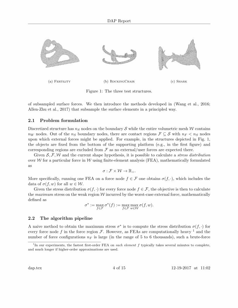
Data. We use the data of three structures (Fig. 1) conveniently denoted as Fertility, Rock-ingChair and Shark. Discretization of structures into finite elements yields thousands ofsurface elements on which external forces can be applied, and the maximum stress across theentire volumetric mesh is sought. The data come from (Ulu et al., 2017).

Methods. We use computationally tractable methods for optimal design in linear models, intro-duced in (Wang et al., 2016; Allen-Zhu et al., 2017). Both methods select a pre-determined num-ber of sample points on the structure surface using only the graph Laplacians of the boundaryelement mesh, without inspecting the stress response that requires computationally expensivefinite-element analysis (FEA).

Results. On the three test structures, our proposed algorithm pipeline uses no more than65 FEAs to successfully recover the maximum stress caused by worst-case external forces. Inaddition, when a 5% to 10% error tolerance is used the number of FEAs can be further reducedto less than 40. This is close to a 100× speed-up compared to the brute-force approach thatperforms FEA on the entire surface mesh, which consists of 4,000 to 6,000 potential force nodes.It also achieves a 5× speed-up over existing work (Ulu et al., 2017) and is also much simpler toimplement.

Keywords: Lightweight structure design, experimental design, linear regressionDAP Committee members:

Aarti Singh 〈aarti@cs.cmu.edu〉 (Machine Learning Department);

dap.tex 1 of 15 12-19-2017 at 11:02

DAP Report

Levent Burak Kara 〈lkara@cmu.edu〉 (Department of Mechanical Engineering);Approved by DAP Committee Chair:

dap.tex 2 of 15 12-19-2017 at 11:02

DAP Report

1 Introduction

As additive manufacturing technologies (also commonly known as 3D printing) become increasinglypopular in recent years, the question of optimization in lightweight structure designs has receivedmuch research attention. Common approach in formalizing such an optimization problem is tomodel the external forces as known and fixed quantities. However, in many real world applica-tions, the external forces, contact locations and magnitudes may change significantly. In order toguarantee that the resulting structure is structurally sound under all possible force configurations,the maximum stress experienced within the current shape hypothesis under the worst-case forceconfiguration is to be predicted at each optimization step. The predicted maximum stress is thencompared against a pre-specified tolerance threshold (i.e., material yield strength) and the structuredesign is then updated accordingly.

Finite-element analysis (FEA) is the standard technique that computes the stress distributionfor a given external force node and the maximum stress suffered can then be subsequently obtained.However, FEA is generally computationally expensive, and performing the FEA on every externalforce configuration possible is out of the question for most structures. Approximation methods thatreduce the total number of FEA runs are mandatory to make the stress prediction and structureoptimization problem feasible in practice.

Ulu et al. (2017) initiated the research of applying machine learning techniques to the maximumstress prediction problem. In particular, a small subset of force locations were sub-sampled andthe stress response on these locations are computed by FEA. Afterwards, a Principle ComponentAnalysis (PCA) quadratic regression model was built on the sub-sampled data points, which wasthen used to predict the stress distribution on the other force configurations not sampled. Empiricalresults show that, with additional post-processing steps, the machine learning based approach givesaccurate predictions of the maximum stress while using much fewer number of FEAs.

In this paper, we improve over the methods in (Ulu et al., 2017) to further reduce the number ofFEAs needed without much sacrifice in the prediction accuracy of the maximum structure stress.We first propose a simplified algorithm pipeline, which replaces the PCA quadratic regression modelin (Ulu et al., 2017) by a simple linear regression model built on the top eigenvectors of the graphLaplacian of the full boundary mesh, and substitutes the local search procedure with a simpleranking post-processing step. Furthermore, we apply the computationally tractable experimentaldesign methods developed in (Wang et al., 2016; Allen-Zhu et al., 2017) to select the sub-sampledtraining set, which improves the naive training set selection algorithm in (Ulu et al., 2017) thatonly maximizes the pairwise geodesic distance between the selected force nodes. Our experimentalresults suggest that the newly proposed algorithm significantly improves over existing work, withapproximately 5× fewer FEAs required compared to (Ulu et al., 2017) and up to 100× comparedagainst the brute-force approach.

2 Problem formulation and methods

In this section we formally formulate the stress prediction problem in lightweight structure designand present a simple pipeline algorithm that produces such a prediction using a small collection

dap.tex 3 of 15 12-19-2017 at 11:02

DAP Report

(a) Fertility (b) RockingChair (c) Shark

Figure 1: The three test structures.

of subsampled surface forces. We then introduce the methods developed in (Wang et al., 2016;Allen-Zhu et al., 2017) that subsample the surface elements in a principled way.

2.1 Problem formulation

Discretized structure has nS nodes on the boundary S while the entire volumetric meshW containsnW nodes. Out of the nS boundary nodes, there are contact regions F ⊆ S with nF < nS nodesupon which external forces might be applied. For example, in the structures depicted in Fig. 1,the objects are fixed from the bottom of the supporting platform (e.g., in the first figure) andcorresponding regions are excluded from F as no external/user forces are expected there.

Given S,F ,W and the current shape hypothesis, it is possible to calculate a stress distributionoverW for a particular force inW using finite-element analysis (FEA), mathematically formulatedas

σ : F ×W → R+.

More specifically, running one FEA on a force node f ∈ F one obtains σ(f, ·), which includes thedata of σ(f, w) for all w ∈ W.

Given the stress distribution σ(f, ·) for every force node f ∈ F , the objective is then to calculatethe maximum stress on the weak regionW incurred by the worst-case external force, mathematicallydefined as

σ∗ := maxf∈F

σ∗(f) := maxf∈F

maxw∈W

σ(f, w).

2.2 The algorithm pipeline

A naive method to obtain the maximum stress σ∗ is to compute the stress distribution σ(f, ·) forevery force node f in the force region F . However, as FEAs are computationally heavy 1 and thenumber of force configurations nF is large (in the range of 5 to 6 thousands), such a brute-force

1In our experiments, the fastest first-order FEA on each element f typically takes several minutes to complete,and much longer if higher-order approximations are used.

dap.tex 4 of 15 12-19-2017 at 11:02

DAP Report

method is infeasible in real-world applications and approximate computations of the maximumstress σ∗ is mandatory.

In this paper, we introduce the following algorithm pipeline that efficiently computes σ∗ usinglinear Laplacian smoothing on a small subset of subsampled force nodes in F . Our algorithmicpipeline is a great simplification of that developed in (Ulu et al., 2017) but yields much morecompetitive results.

Subsampling of force nodes. The algorithm pipeline starts with sampling a small subset ofthe contact region FL ⊆ F such that FL contains nFL � nF force nodes. The subsampling canbe accomplished by simple uniform or leverage score sampling (Drineas et al., 2008; Spielman &Srivastava, 2011), or more sophisticated methods such as the k-means algorithm (Ulu et al., 2017)and the computationally efficient algorithms proposed in (Wang et al., 2016; Allen-Zhu et al., 2017).After FL is obtained, FEA is performed on the nFL subsampled force nodes to obtain the criticalstress map σ(f, ·) as well as the maximum stress σ∗(f) for all f ∈ FL.

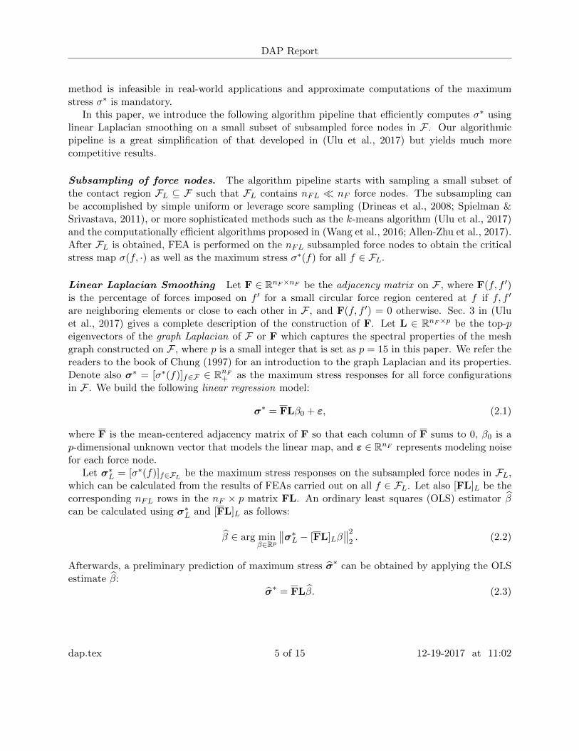
Linear Laplacian Smoothing Let F ∈ RnF×nF be the adjacency matrix on F , where F(f, f ′)is the percentage of forces imposed on f ′ for a small circular force region centered at f if f, f ′

are neighboring elements or close to each other in F , and F(f, f ′) = 0 otherwise. Sec. 3 in (Uluet al., 2017) gives a complete description of the construction of F. Let L ∈ RnF×p be the top-peigenvectors of the graph Laplacian of F or F which captures the spectral properties of the meshgraph constructed on F , where p is a small integer that is set as p = 15 in this paper. We refer thereaders to the book of Chung (1997) for an introduction to the graph Laplacian and its properties.Denote also σ∗ = [σ∗(f)]f∈F ∈ RnF

+ as the maximum stress responses for all force configurationsin F . We build the following linear regression model:

σ∗ = FLβ0 + ε, (2.1)

where F is the mean-centered adjacency matrix of F so that each column of F sums to 0, β0 is ap-dimensional unknown vector that models the linear map, and ε ∈ RnF represents modeling noisefor each force node.

Let σ∗L = [σ∗(f)]f∈FLbe the maximum stress responses on the subsampled force nodes in FL,

which can be calculated from the results of FEAs carried out on all f ∈ FL. Let also [FL]L be thecorresponding nFL rows in the nF × p matrix FL. An ordinary least squares (OLS) estimator β̂can be calculated using σ∗L and [FL]L as follows:

β̂ ∈ arg minβ∈Rp

∥∥σ∗L − [FL]Lβ∥∥2

2. (2.2)

Afterwards, a preliminary prediction of maximum stress σ̂∗ can be obtained by applying the OLSestimate β̂:

σ̂∗ = FLβ̂. (2.3)

dap.tex 5 of 15 12-19-2017 at 11:02

DAP Report

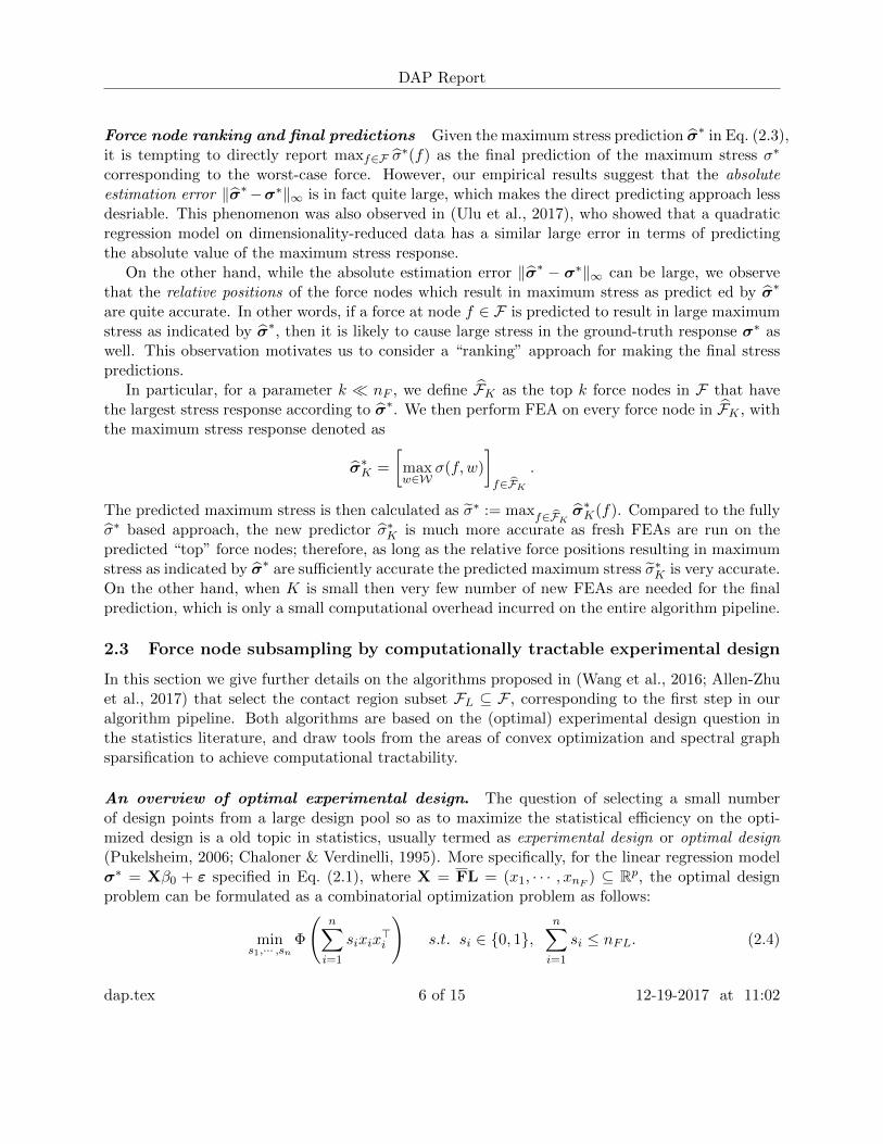
Force node ranking and final predictions Given the maximum stress prediction σ̂∗ in Eq. (2.3),it is tempting to directly report maxf∈F σ̂

∗(f) as the final prediction of the maximum stress σ∗

corresponding to the worst-case force. However, our empirical results suggest that the absoluteestimation error ‖σ̂∗−σ∗‖∞ is in fact quite large, which makes the direct predicting approach lessdesriable. This phenomenon was also observed in (Ulu et al., 2017), who showed that a quadraticregression model on dimensionality-reduced data has a similar large error in terms of predictingthe absolute value of the maximum stress response.

On the other hand, while the absolute estimation error ‖σ̂∗ − σ∗‖∞ can be large, we observethat the relative positions of the force nodes which result in maximum stress as predict ed by σ̂∗

are quite accurate. In other words, if a force at node f ∈ F is predicted to result in large maximumstress as indicated by σ̂∗, then it is likely to cause large stress in the ground-truth response σ∗ aswell. This observation motivates us to consider a “ranking” approach for making the final stresspredictions.

In particular, for a parameter k � nF , we define F̂K as the top k force nodes in F that havethe largest stress response according to σ̂∗. We then perform FEA on every force node in F̂K , withthe maximum stress response denoted as

σ̂∗K =

[maxw∈W

σ(f, w)

]f∈F̂K

.

The predicted maximum stress is then calculated as σ̃∗ := maxf∈F̂K

σ̂∗K(f). Compared to the fullyσ̂∗ based approach, the new predictor σ̂∗K is much more accurate as fresh FEAs are run on thepredicted “top” force nodes; therefore, as long as the relative force positions resulting in maximumstress as indicated by σ̂∗ are sufficiently accurate the predicted maximum stress σ̃∗K is very accurate.On the other hand, when K is small then very few number of new FEAs are needed for the finalprediction, which is only a small computational overhead incurred on the entire algorithm pipeline.

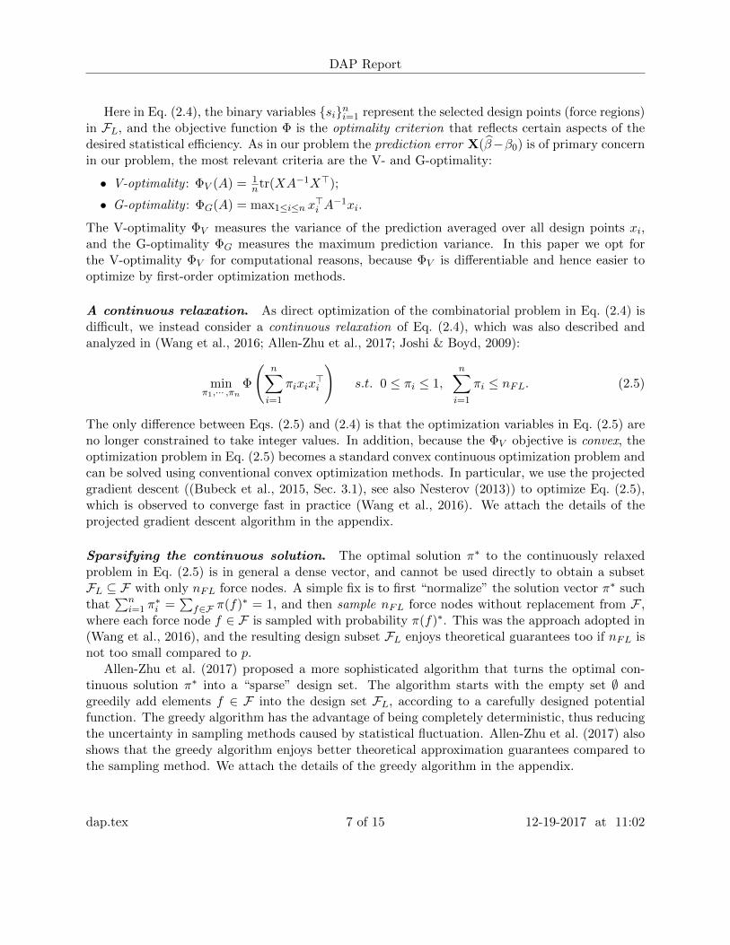
2.3 Force node subsampling by computationally tractable experimental design

In this section we give further details on the algorithms proposed in (Wang et al., 2016; Allen-Zhuet al., 2017) that select the contact region subset FL ⊆ F , corresponding to the first step in ouralgorithm pipeline. Both algorithms are based on the (optimal) experimental design question inthe statistics literature, and draw tools from the areas of convex optimization and spectral graphsparsification to achieve computational tractability.

An overview of optimal experimental design. The question of selecting a small numberof design points from a large design pool so as to maximize the statistical efficiency on the opti-mized design is a old topic in statistics, usually termed as experimental design or optimal design(Pukelsheim, 2006; Chaloner & Verdinelli, 1995). More specifically, for the linear regression modelσ∗ = Xβ0 + ε specified in Eq. (2.1), where X = FL = (x1, · · · , xnF ) ⊆ Rp, the optimal designproblem can be formulated as a combinatorial optimization problem as follows:

mins1,··· ,sn

Φ

(n∑i=1

sixix>i

)s.t. si ∈ {0, 1},

n∑i=1

si ≤ nFL. (2.4)

dap.tex 6 of 15 12-19-2017 at 11:02

DAP Report

Here in Eq. (2.4), the binary variables {si}ni=1 represent the selected design points (force regions)in FL, and the objective function Φ is the optimality criterion that reflects certain aspects of thedesired statistical efficiency. As in our problem the prediction error X(β̂−β0) is of primary concernin our problem, the most relevant criteria are the V- and G-optimality:

• V-optimality : ΦV (A) = 1ntr(XA−1X>);

• G-optimality : ΦG(A) = max1≤i≤n x>i A−1xi.

The V-optimality ΦV measures the variance of the prediction averaged over all design points xi,and the G-optimality ΦG measures the maximum prediction variance. In this paper we opt forthe V-optimality ΦV for computational reasons, because ΦV is differentiable and hence easier tooptimize by first-order optimization methods.

A continuous relaxation. As direct optimization of the combinatorial problem in Eq. (2.4) isdifficult, we instead consider a continuous relaxation of Eq. (2.4), which was also described andanalyzed in (Wang et al., 2016; Allen-Zhu et al., 2017; Joshi & Boyd, 2009):

minπ1,··· ,πn

Φ

(n∑i=1

πixix>i

)s.t. 0 ≤ πi ≤ 1,

n∑i=1

πi ≤ nFL. (2.5)

The only difference between Eqs. (2.5) and (2.4) is that the optimization variables in Eq. (2.5) areno longer constrained to take integer values. In addition, because the ΦV objective is convex, theoptimization problem in Eq. (2.5) becomes a standard convex continuous optimization problem andcan be solved using conventional convex optimization methods. In particular, we use the projectedgradient descent ((Bubeck et al., 2015, Sec. 3.1), see also Nesterov (2013)) to optimize Eq. (2.5),which is observed to converge fast in practice (Wang et al., 2016). We attach the details of theprojected gradient descent algorithm in the appendix.

Sparsifying the continuous solution. The optimal solution π∗ to the continuously relaxedproblem in Eq. (2.5) is in general a dense vector, and cannot be used directly to obtain a subsetFL ⊆ F with only nFL force nodes. A simple fix is to first “normalize” the solution vector π∗ suchthat

∑ni=1 π

∗i =

∑f∈F π(f)∗ = 1, and then sample nFL force nodes without replacement from F ,

where each force node f ∈ F is sampled with probability π(f)∗. This was the approach adopted in(Wang et al., 2016), and the resulting design subset FL enjoys theoretical guarantees too if nFL isnot too small compared to p.

Allen-Zhu et al. (2017) proposed a more sophisticated algorithm that turns the optimal con-tinuous solution π∗ into a “sparse” design set. The algorithm starts with the empty set ∅ andgreedily add elements f ∈ F into the design set FL, according to a carefully designed potentialfunction. The greedy algorithm has the advantage of being completely deterministic, thus reducingthe uncertainty in sampling methods caused by statistical fluctuation. Allen-Zhu et al. (2017) alsoshows that the greedy algorithm enjoys better theoretical approximation guarantees compared tothe sampling method. We attach the details of the greedy algorithm in the appendix.

dap.tex 7 of 15 12-19-2017 at 11:02

DAP Report

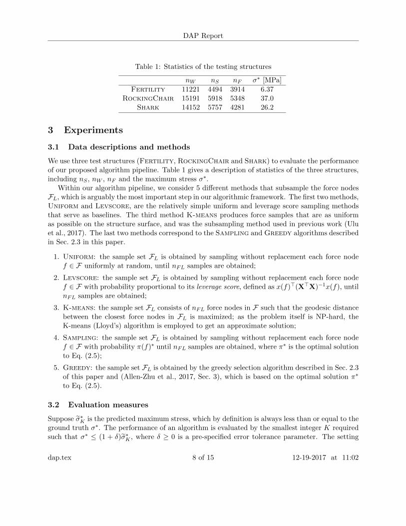
Table 1: Statistics of the testing structures

nW nS nF σ∗ [MPa]

Fertility 11221 4494 3914 6.37RockingChair 15191 5918 5348 37.0

Shark 14152 5757 4281 26.2

3 Experiments

3.1 Data descriptions and methods

We use three test structures (Fertility, RockingChair and Shark) to evaluate the performanceof our proposed algorithm pipeline. Table 1 gives a description of statistics of the three structures,including nS , nW , nF and the maximum stress σ∗.

Within our algorithm pipeline, we consider 5 different methods that subsample the force nodesFL, which is arguably the most important step in our algorithmic framework. The first two methods,Uniform and Levscore, are the relatively simple uniform and leverage score sampling methodsthat serve as baselines. The third method K-means produces force samples that are as uniformas possible on the structure surface, and was the subsampling method used in previous work (Uluet al., 2017). The last two methods correspond to the Sampling and Greedy algorithms describedin Sec. 2.3 in this paper.

1. Uniform: the sample set FL is obtained by sampling without replacement each force nodef ∈ F uniformly at random, until nFL samples are obtained;

2. Levscore: the sample set FL is obtained by sampling without replacement each force nodef ∈ F with probability proportional to its leverage score, defined as x(f)>(X>X)−1x(f), untilnFL samples are obtained;

3. K-means: the sample set FL consists of nFL force nodes in F such that the geodesic distancebetween the closest force nodes in FL is maximized; as the problem itself is NP-hard, theK-means (Lloyd’s) algorithm is employed to get an approximate solution;

4. Sampling: the sample set FL is obtained by sampling without replacement each force nodef ∈ F with probability π(f)∗ until nFL samples are obtained, where π∗ is the optimal solutionto Eq. (2.5);

5. Greedy: the sample set FL is obtained by the greedy selection algorithm described in Sec. 2.3of this paper and (Allen-Zhu et al., 2017, Sec. 3), which is based on the optimal solution π∗

to Eq. (2.5).

3.2 Evaluation measures

Suppose σ̃∗K is the predicted maximum stress, which by definition is always less than or equal to theground truth σ∗. The performance of an algorithm is evaluated by the smallest integer K requiredsuch that σ∗ ≤ (1 + δ)σ̃∗K , where δ ≥ 0 is a pre-specified error tolerance parameter. The setting

dap.tex 8 of 15 12-19-2017 at 11:02

DAP Report

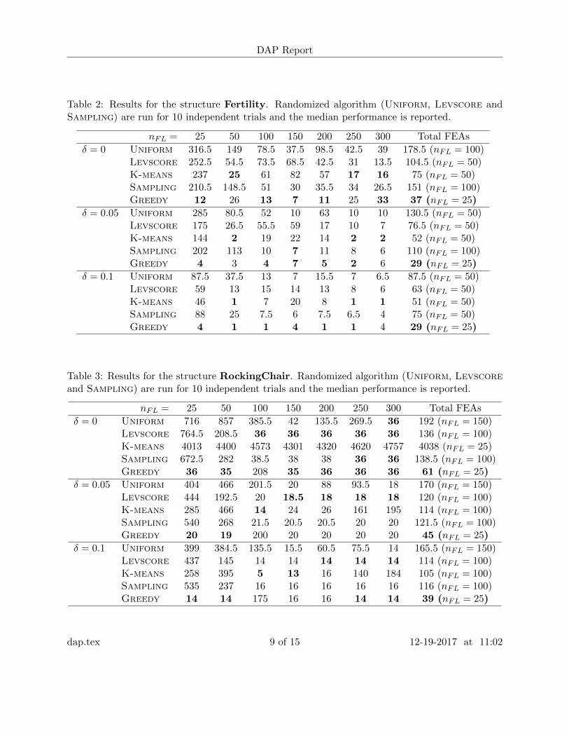
Table 2: Results for the structure Fertility. Randomized algorithm (Uniform, Levscore andSampling) are run for 10 independent trials and the median performance is reported.

nFL = 25 50 100 150 200 250 300 Total FEAs

δ = 0 Uniform 316.5 149 78.5 37.5 98.5 42.5 39 178.5 (nFL = 100)Levscore 252.5 54.5 73.5 68.5 42.5 31 13.5 104.5 (nFL = 50)K-means 237 25 61 82 57 17 16 75 (nFL = 50)Sampling 210.5 148.5 51 30 35.5 34 26.5 151 (nFL = 100)Greedy 12 26 13 7 11 25 33 37 (nFL = 25)

δ = 0.05 Uniform 285 80.5 52 10 63 10 10 130.5 (nFL = 50)Levscore 175 26.5 55.5 59 17 10 7 76.5 (nFL = 50)K-means 144 2 19 22 14 2 2 52 (nFL = 50)Sampling 202 113 10 7 11 8 6 110 (nFL = 100)Greedy 4 3 4 7 5 2 6 29 (nFL = 25)

δ = 0.1 Uniform 87.5 37.5 13 7 15.5 7 6.5 87.5 (nFL = 50)Levscore 59 13 15 14 13 8 6 63 (nFL = 50)K-means 46 1 7 20 8 1 1 51 (nFL = 50)Sampling 88 25 7.5 6 7.5 6.5 4 75 (nFL = 50)Greedy 4 1 1 4 1 1 4 29 (nFL = 25)

Table 3: Results for the structure RockingChair. Randomized algorithm (Uniform, Levscoreand Sampling) are run for 10 independent trials and the median performance is reported.

nFL = 25 50 100 150 200 250 300 Total FEAs

δ = 0 Uniform 716 857 385.5 42 135.5 269.5 36 192 (nFL = 150)Levscore 764.5 208.5 36 36 36 36 36 136 (nFL = 100)K-means 4013 4400 4573 4301 4320 4620 4757 4038 (nFL = 25)Sampling 672.5 282 38.5 38 38 36 36 138.5 (nFL = 100)Greedy 36 35 208 35 36 36 36 61 (nFL = 25)

δ = 0.05 Uniform 404 466 201.5 20 88 93.5 18 170 (nFL = 150)Levscore 444 192.5 20 18.5 18 18 18 120 (nFL = 100)K-means 285 466 14 24 26 161 195 114 (nFL = 100)Sampling 540 268 21.5 20.5 20.5 20 20 121.5 (nFL = 100)Greedy 20 19 200 20 20 20 20 45 (nFL = 25)

δ = 0.1 Uniform 399 384.5 135.5 15.5 60.5 75.5 14 165.5 (nFL = 150)Levscore 437 145 14 14 14 14 14 114 (nFL = 100)K-means 258 395 5 13 16 140 184 105 (nFL = 100)Sampling 535 237 16 16 16 16 16 116 (nFL = 100)Greedy 14 14 175 16 16 14 14 39 (nFL = 25)

dap.tex 9 of 15 12-19-2017 at 11:02

DAP Report

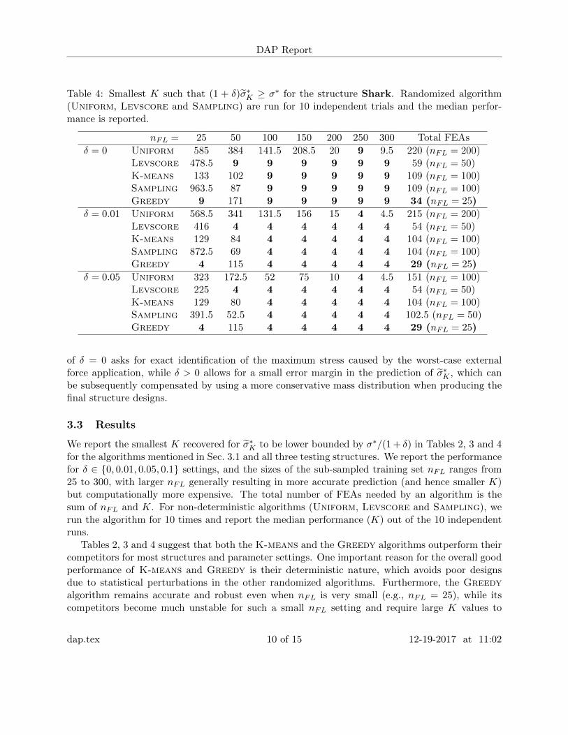
Table 4: Smallest K such that (1 + δ)σ̃∗K ≥ σ∗ for the structure Shark. Randomized algorithm(Uniform, Levscore and Sampling) are run for 10 independent trials and the median perfor-mance is reported.

nFL = 25 50 100 150 200 250 300 Total FEAs

δ = 0 Uniform 585 384 141.5 208.5 20 9 9.5 220 (nFL = 200)Levscore 478.5 9 9 9 9 9 9 59 (nFL = 50)K-means 133 102 9 9 9 9 9 109 (nFL = 100)Sampling 963.5 87 9 9 9 9 9 109 (nFL = 100)Greedy 9 171 9 9 9 9 9 34 (nFL = 25)

δ = 0.01 Uniform 568.5 341 131.5 156 15 4 4.5 215 (nFL = 200)Levscore 416 4 4 4 4 4 4 54 (nFL = 50)K-means 129 84 4 4 4 4 4 104 (nFL = 100)Sampling 872.5 69 4 4 4 4 4 104 (nFL = 100)Greedy 4 115 4 4 4 4 4 29 (nFL = 25)

δ = 0.05 Uniform 323 172.5 52 75 10 4 4.5 151 (nFL = 100)Levscore 225 4 4 4 4 4 4 54 (nFL = 50)K-means 129 80 4 4 4 4 4 104 (nFL = 100)Sampling 391.5 52.5 4 4 4 4 4 102.5 (nFL = 50)Greedy 4 115 4 4 4 4 4 29 (nFL = 25)

of δ = 0 asks for exact identification of the maximum stress caused by the worst-case externalforce application, while δ > 0 allows for a small error margin in the prediction of σ̃∗K , which canbe subsequently compensated by using a more conservative mass distribution when producing thefinal structure designs.

3.3 Results

We report the smallest K recovered for σ̃∗K to be lower bounded by σ∗/(1 + δ) in Tables 2, 3 and 4for the algorithms mentioned in Sec. 3.1 and all three testing structures. We report the performancefor δ ∈ {0, 0.01, 0.05, 0.1} settings, and the sizes of the sub-sampled training set nFL ranges from25 to 300, with larger nFL generally resulting in more accurate prediction (and hence smaller K)but computationally more expensive. The total number of FEAs needed by an algorithm is thesum of nFL and K. For non-deterministic algorithms (Uniform, Levscore and Sampling), werun the algorithm for 10 times and report the median performance (K) out of the 10 independentruns.

Tables 2, 3 and 4 suggest that both the K-means and the Greedy algorithms outperform theircompetitors for most structures and parameter settings. One important reason for the overall goodperformance of K-means and Greedy is their deterministic nature, which avoids poor designsdue to statistical perturbations in the other randomized algorithms. Furthermore, the Greedyalgorithm remains accurate and robust even when nFL is very small (e.g., nFL = 25), while itscompetitors become much unstable for such a small nFL setting and require large K values to

dap.tex 10 of 15 12-19-2017 at 11:02

DAP Report

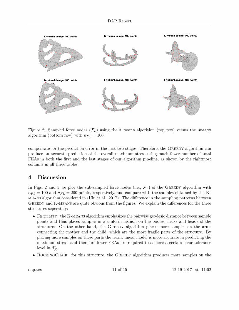
Figure 2: Sampled force nodes (FL) using the K-means algorithm (top row) versus the Greedy

algorithm (bottom row) with nFL = 100.

compensate for the prediction error in the first two stages. Therefore, the Greedy algorithm canproduce an accurate prediction of the overall maximum stress using much fewer number of totalFEAs in both the first and the last stages of our algorithm pipeline, as shown by the rightmostcolumns in all three tables.

4 Discussion

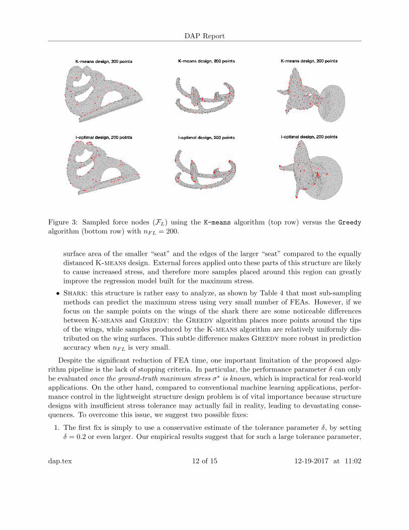
In Figs. 2 and 3 we plot the sub-sampled force nodes (i.e., FL) of the Greedy algorithm withnFL = 100 and nFL = 200 points, respectively, and compare with the samples obtained by the K-means algorithm considered in (Ulu et al., 2017). The difference in the sampling patterns betweenGreedy and K-means are quite obvious from the figures. We explain the differences for the threestructures seperately:

• Fertility: the K-means algorithm emphasizes the pairwise geodesic distance between samplepoints and thus places samples in a uniform fashion on the bodies, necks and heads of thestructure. On the other hand, the Greedy algorithm places more samples on the armsconnecting the mother and the child, which are the most fragile parts of the structure. Byplacing more samples on these parts the learnt linear model is more accurate in predicting themaximum stress, and therefore fewer FEAs are required to achieve a certain error tolerancelevel in σ̃∗K .

• RockingChair: for this structure, the Greedy algorithm produces more samples on the

dap.tex 11 of 15 12-19-2017 at 11:02

DAP Report

Figure 3: Sampled force nodes (FL) using the K-means algorithm (top row) versus the Greedy

algorithm (bottom row) with nFL = 200.

surface area of the smaller “seat” and the edges of the larger “seat” compared to the equallydistanced K-means design. External forces applied onto these parts of this structure are likelyto cause increased stress, and therefore more samples placed around this region can greatlyimprove the regression model built for the maximum stress.

• Shark: this structure is rather easy to analyze, as shown by Table 4 that most sub-samplingmethods can predict the maximum stress using very small number of FEAs. However, if wefocus on the sample points on the wings of the shark there are some noticeable differencesbetween K-means and Greedy: the Greedy algorithm places more points around the tipsof the wings, while samples produced by the K-means algorithm are relatively uniformly dis-tributed on the wing surfaces. This subtle difference makes Greedy more robust in predictionaccuracy when nFL is very small.

Despite the significant reduction of FEA time, one important limitation of the proposed algo-rithm pipeline is the lack of stopping criteria. In particular, the performance parameter δ can onlybe evaluated once the ground-truth maximum stress σ∗ is known, which is impractical for real-worldapplications. On the other hand, compared to conventional machine learning applications, perfor-mance control in the lightweight structure design problem is of vital importance because structuredesigns with insufficient stress tolerance may actually fail in reality, leading to devastating conse-quences. To overcome this issue, we suggest two possible fixes:

1. The first fix is simply to use a conservative estimate of the tolerance parameter δ, by settingδ = 0.2 or even larger. Our empirical results suggest that for such a large tolerance parameter,

dap.tex 12 of 15 12-19-2017 at 11:02

DAP Report

K = 20 is sufficient for almost all structures. The disadvantage of this strategy however isthe loss of material efficiency, as a δ = 0.2 error margin might be too conservative and requiremuch more material mass on the structure. In addition, it is possible that for especiallychallenging/pathological structures, even a δ = 0.2 margin might be insufficient.

2. A more principled method is to use cross validation to obtain an estimate on the accuracyof the predicted maximum stress σ̃∗K . More specifically, we start with a pre-fixed toleranceparameter δ and an initial small sample set FL. We then divide the FL into disjoint trainingand testing sets, and obtain an estimated tolerance δ̂. If δ̂ is larger than δ desired, we concludethat the current samples are not sufficient to build a model that matches the desired accuracy,and nFL is subsequently increased to obtain more data such that a more accurate model canbe built. This process can be repeated until the cross-validated tolerance δ̂ decreases to thespecified tolerance level δ.

A The projected gradient descent algorithm

Using the V -optimality ΦV (A) = tr(XA−1X>), the partial derivative of ΦV with respect to πi canbe calculated as

∂ΦV

∂πi= − 1

nx>i Σ−1X>XΣ−1xi, (A.1)

where Σ =∑n

j=1 πixix>i . Let also Π := {π ∈ Rn : 0 ≤ πi ≤ 1,

∑ni=1 πi ≤ nFL} be the feasible set.

The projected gradient descent algorithm can then be formulated as following:

1. Input: X ∈ RnF×p, feasibility set Π, algorithm parameters α ∈ (0, 1/2], β ∈ (0, 1);

2. Initialization: π(0) = (nFL/nF , · · · , nFL/nF ), t = 0;

3. While stopping criteria are not met do the following:

(a) Compute the gradient gt = ∇πΦ(π(t)) using Eq. (A.1);

(b) Find the smallest integer s ≥ 0 such that Φ(π) − Φ(π(t)) ≤ αg>t (π − π(t)), where π =PΠ(π(t) − βsgt);

(c) Update: π(t+1) = PΠ(π(t) − βsgt), t← t+ 1.

Here in Steps 3(b) and 3(c), the PΠ(·) is the projection operator onto the (convex) constrain setΠ in Euclidean norm. More specifically, PΠ(π) := arg minz∈Π ‖π − z‖2. Such projection can beefficiently computed in almost linear time up to high accuracy (Wang et al. (2016), see also Duchiet al. (2008); Condat (2015); Su et al. (2012)). Also, the step 3(b) corresponds to the Amijo’srule (also known as backtracking line search) that automatically selects step sizes, a popular andefficient method for step size selection in full gradient descent methods.

B The Greedy algorithm

The Greedy algorithm was proposed in (Allen-Zhu et al., 2017) as a principled method to sparsifythe continuous optimization solution π∗. The algorithm makes uses of a carefully designed potential

dap.tex 13 of 15 12-19-2017 at 11:02

DAP Report

function for i ∈ [nF ] and Λ ⊆ [nF ]:

ψ(i; Λ) :=x>i B(Λ)xi

1 + αx>i B(Λ)1/2xiwhere B(Λ) =

cI +∑j∈Λ

xjx>j

−2

, tr(B(Λ)) = 1. (B.1)

Here α > 0 is an algorithm parameter that can be tuned, and c ∈ R is the unique real numbersuch that tr(B(Λ)) = 1. The exact values of c can be computed efficiently using a binary searchprocedure, as shown in (Allen-Zhu et al., 2017). The potential function is inspired by a regretminimization interpretation of the least singular values of sum of rank-1 matrices. Interestedreaders should refer to (Allen-Zhu et al., 2017; Silva et al., 2016; Allen-Zhu et al., 2015) for moredetails and motivations.

Based on the potential function in Eq. (B.1), the Greedy algorithm starts with an empty setand add force nodes one by one in a greedy manner, until there are nFL elements in FL.

1. Input: X ∈ RnF×p, budget nFL, optimal solution π∗, algorithm parameter α > 0;

2. Whitening: X← X(XΣ∗X>)−1/2, where Σ∗ =

∑ni=1 π

∗i xix

>i ;

3. Initialization: Λ0 = ∅, FL = ∅;4. For t = 1 to nFL do the following:

(a) Compute ψ(i; Λt−1) for all i /∈ Λt−1 and select it := arg maxi/∈Λt−1ψ(i; Λt−1);

(b) Update: Λt = Λt−1 ∪ {it}, FL ← FL ∪ {it}.

Acknowledgement

I would like to thank Erva Ulu for preparing the data and offering great help in data analysis. Ialso thank my DAP advisors Aarti Singh and Levent Burak Kara for their valuable suggestions.This research was supported in part by NSF CCF-1563918 and AFRL FA87501720212.

References

Allen-Zhu, Z., Li, Y., Singh, A., & Wang, Y. (2017). Near-optimal design of experiments via regretminimization. In Proceedings of the International Conference on Machine Learning (ICML).

Allen-Zhu, Z., Liao, Z., & Orecchia, L. (2015). Spectral sparsification and regret minimizationbeyond matrix multiplicative updates. In Proceedings of Annual Symposium on the Theory ofComputing (STOC).

Bubeck, S., et al. (2015). Convex optimization: Algorithms and complexity. Foundations andTrends R© in Machine Learning , 8 (3-4), 231–357.

Chaloner, K., & Verdinelli, I. (1995). Bayesian experimental design: A review. Statistical Science,10 (3), 273–304.

dap.bbl 14 of 15 12-19-2017 at 11:02

DAP Report

Chung, F. R. (1997). Spectral graph theory . 92. American Mathematical Soc.

Condat, L. (2015). Fast projection onto the simplex and the L1-ball. Mathematical Programming(Series A), 158 , 575–585.

Drineas, P., Mahoney, M. W., & Muthukrishnan, S. (2008). Relative-error CUR matrix decompo-sitions. SIAM Journal on Matrix Analysis and Applications, 30 (2), 844–881.

Duchi, J., Shalev-Shwartz, S., Singer, Y., & Chandra, T. (2008). Efficient projections onto theL1-ball for learning in high dimensions. In Proceedings of International Conference on Machinelearning (ICML).

Joshi, S., & Boyd, S. (2009). Sensor selection via convex optimization. IEEE Transactions onSignal Processing , 57 (2), 451–462.

Nesterov, Y. (2013). Introductory lectures on convex optimization: A basic course, vol. 87. SpringerScience & Business Media.

Pukelsheim, F. (2006). Optimal design of experiments. SIAM.

Silva, M. K., Harvey, N. J., & Sato, C. M. (2016). Sparse sums of positive semidefinite matrices.ACM Transactions on Algorithms, 12 (1), 9.

Spielman, D. A., & Srivastava, N. (2011). Graph sparsification by effective resistances. SIAMJournal on Computing , 40 (6), 1913–1926.

Su, H., Yu, A. W., & Li, F.-F. (2012). Efficient euclidean projections onto the intersection of normballs. In Proceedings of International Conference on Machine Learning (ICML).

Ulu, E., Mccann, J., & Kara, L. B. (2017). Lightweight structure design under force locationuncertainty. ACM Transactions on Graphics (TOG), 36 (4), 158.

Wang, Y., Yu, W. A., & Singh, A. (2016). On computationally tractable selection of experimentsin regression models. arXiv preprints: arXiv:1601.02068 .

dap.tex 15 of 15 12-19-2017 at 11:02