Embed Size (px)
Citation preview
Analysis of Variance | Chapter 4 | Extal. Design and Their Analysis | Shalabh, IIT Kanpur 1 1
Chapter 4
Experimental Design and Their Analysis
Design of experiment means how to design an experiment in the sense that how the observations or
measurements should be obtained to answer a query in a valid, efficient and economical way. The designing
of experiment and the analysis of obtained data are inseparable. If the experiment is designed properly
keeping in mind the question, then the data generated is valid and proper analysis of data provides the valid
statistical inferences. If the experiment is not well designed, the validity of the statistical inferences is
questionable and may be invalid.
It is important to understand first the basic terminologies used in the experimental design.
Experimental unit: For conducting an experiment, the experimental material is divided into smaller parts and each part is
referred to as experimental unit. The experimental unit is randomly assigned to a treatment is the
experimental unit. The phrase “randomly assigned” is very important in this definition.
Experiment: A way of getting an answer to a question which the experimenter wants to know.
Treatment Different objects or procedures which are to be compared in an experiment are called treatments.
Sampling unit: The object that is measured in an experiment is called the sampling unit. This may be different from the
experimental unit.
Factor: A factor is a variable defining a categorization. A factor can be fixed or random in nature. A factor is termed
as fixed factor if all the levels of interest are included in the experiment.
A factor is termed as random factor if all the levels of interest are not included in the experiment and those
that are can be considered to be randomly chosen from all the levels of interest.
Replication: It is the repetition of the experimental situation by replicating the experimental unit.
Analysis of Variance | Chapter 4 | Extal. Design and Their Analysis | Shalabh, IIT Kanpur 2 2
Experimental error: The unexplained random part of variation in any experiment is termed as experimental error. An estimate
of experimental error can be obtained by replication.
Treatment design: A treatment design is the manner in which the levels of treatments are arranged in an experiment.
Example: (Ref.: Statistical Design, G. Casella, Chapman and Hall, 2008)
Suppose some varieties of fish food is to be investigated on some species of fishes. The food is placed in
the water tanks containing the fishes. The response is the increase in the weight of fish. The experimental
unit is the tank, as the treatment is applied to the tank, not to the fish. Note that if the experimenter had taken
the fish in hand and placed the food in the mouth of fish, then the fish would have been the experimental
unit as long as each of the fish got an independent scoop of food.
Design of experiment: One of the main objectives of designing an experiment is how to verify the hypothesis in an efficient and
economical way. In the contest of the null hypothesis of equality of several means of normal populations
having same variances, the analysis of variance technique can be used. Note that such techniques are based
on certain statistical assumptions. If these assumptions are violated, the outcome of the test of hypothesis
then may also be faulty and the analysis of data may be meaningless. So the main question is how to obtain
the data such that the assumptions are met and the data is readily available for the application of tools like
analysis of variance. The designing of such mechanism to obtain such data is achieved by the design of
experiment. After obtaining the sufficient experimental unit, the treatments are allocated to the
experimental units in a random fashion. Design of experiment provides a method by which the treatments
are placed at random on the experimental units in such a way that the responses are estimated with the
utmost precision possible.
Principles of experimental design: There are three basic principles of design which were developed by Sir Ronald A. Fisher.
(i) Randomization
(ii) Replication
(iii) Local control
Analysis of Variance | Chapter 4 | Extal. Design and Their Analysis | Shalabh, IIT Kanpur 3 3
(i) Randomization The principle of randomization involves the allocation of treatment to experimental units at random to
avoid any bias in the experiment resulting from the influence of some extraneous unknown factor that
may affect the experiment. In the development of analysis of variance, we assume that the errors are
random and independent. In turn, the observations also become random. The principle of randomization
ensures this.
The random assignment of experimental units to treatments results in the following outcomes.
a) It eliminates the systematic bias.
b) It is needed to obtain a representative sample from the population.
c) It helps in distributing the unknown variation due to confounded variables throughout the
experiment and breaks the confounding influence.
Randomization forms a basis of valid experiment but replication is also needed for the validity of the
experiment.
If the randomization process is such that every experimental unit has an equal chance of receiving each
treatment, it is called a complete randomization.
(ii) Replication: In the replication principle, any treatment is repeated a number of times to obtain a valid and more
reliable estimate than which is possible with one observation only. Replication provides an efficient way
of increasing the precision of an experiment. The precision increases with the increase in the number of
observations. Replication provides more observations when the same treatment is used, so it increases
precision. For example, if variance of x is 2σ than variance of sample mean x based on n observation
is 2
.nσ
So as n increases, ( )Var x decreases.
(ii) Local control (error control) The replication is used with local control to reduce the experimental error. For example, if the
experimental units are divided into different groups such that they are homogeneous within the blocks,
than the variation among the blocks is eliminated and ideally the error component will contain the
variation due to the treatments only. This will in turn increase the efficiency.

Analysis of Variance | Chapter 4 | Extal. Design and Their Analysis | Shalabh, IIT Kanpur 4 4
Complete and incomplete block designs: In most of the experiments, the available experimental units are grouped into blocks having more or less
identical characteristics to remove the blocking effect from the experimental error. Such design are termed
as block designs.
The number of experimental units in a block is called the block size.
If
size of block = number of treatments
and
each treatment in each block is randomly allocated,
then it is a full replication and the design is called as complete block design.
In case, the number of treatments is so large that a full replication in each block makes it too heterogeneous
with respect to the characteristic under study, then smaller but homogeneous blocks can be used. In such a
case, the blocks do not contain a full replicate of the treatments. Experimental designs with blocks
containing an incomplete replication of the treatments are called incomplete block designs.
Completely randomized design (CRD) The CRD is the simplest design. Suppose there are v treatments to be compared.
• All experimental units are considered the same and no division or grouping among them exist.
• In CRD, the v treatments are allocated randomly to the whole set of experimental units, without
making any effort to group the experimental units in any way for more homogeneity.
• Design is entirely flexible in the sense that any number of treatments or replications may be used.
• Number of replications for different treatments need not be equal and may vary from treatment to
treatment depending on the knowledge (if any) on the variability of the observations on individual
treatments as well as on the accuracy required for the estimate of individual treatment effect.
Example: Suppose there are 4 treatments and 20 experimental units, then
- the treatment 1 is replicated, say 3 times and is given to 3 experimental units,
- the treatment 2 is replicated, say 5 times and is given to 5 experimental units,
- the treatment 3 is replicated, say 6 times and is given to 6 experimental units
and
- finally, the treatment 4 is replicated [20-(6+5+3)=]6 times and is given to the remaining 6
experimental units

Analysis of Variance | Chapter 4 | Extal. Design and Their Analysis | Shalabh, IIT Kanpur 5 5
• All the variability among the experimental units goes into experimented error.
• CRD is used when the experimental material is homogeneous.
• CRD is often inefficient.
• CRD is more useful when the experiments are conducted inside the lab.
• CRD is well suited for the small number of treatments and for the homogeneous experimental
material.
Layout of CRD
Following steps are needed to design a CRD:
Divide the entire experimental material or area into a number of experimental units, say n.
Fix the number of replications for different treatments in advance (for given total number of
available experimental units).
No local control measure is provided as such except that the error variance can be reduced by
choosing a homogeneous set of experimental units.
Procedure
Let the v treatments are numbered from 1,2,...,v and in be the number of replications required for ith
treatment such that 1
.v
ii
n n=
=∑
Select 1n units out of n units randomly and apply treatment 1 to these 1n units.
(Note: This is how the randomization principle is utilized is CRD.)
Select 2n units out of ( 1)n n− units randomly and apply treatment 2 to these 2n units.
Continue with this procedure until all the treatments have been utilized.
Generally equal number of treatments are allocated to all the experimental units unless no practical
limitation dictates or some treatments are more variable or/and of more interest.
Analysis There is only one factor which is affecting the outcome – treatment effect. So the set-up of one-way analysis
of variance is to be used.
:ijy Individual measurement of jth experimental units for ith treatment i = 1,2,...,v , j = 1,2,..., in .
:ijy Independently distributed following 2( , )iN µ α σ+ with 1
0v
i ii
nα=
=∑ .
µ : overall mean
Analysis of Variance | Chapter 4 | Extal. Design and Their Analysis | Shalabh, IIT Kanpur 6 6
iα : ith treatment effect
0 1 2: ... 0vH α α α= = = =
1 :H All 'i sα are not equal.
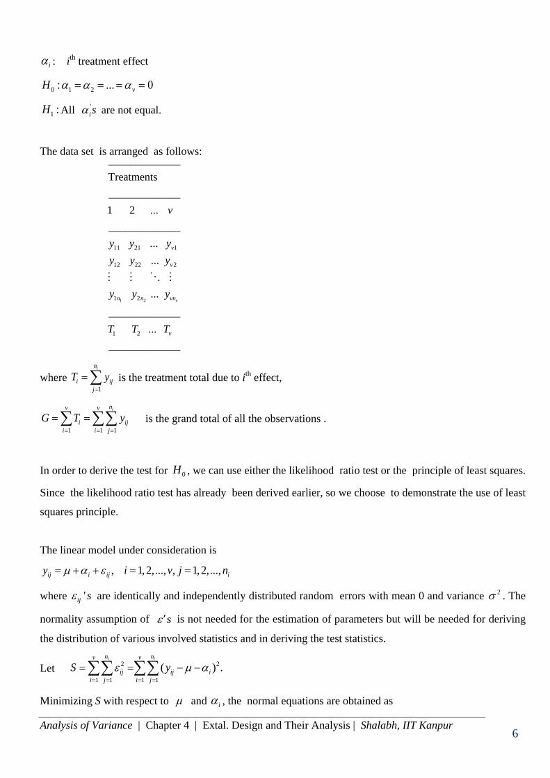
The data set is arranged as follows:
1 2
11 21 1
12 22 2
1 2
1 2
_____________Treatments_____________1 2 ... _____________
... ... ...
_____________...
_____________
v
v
v
n n vn
v
v
y y yy y y
y y y
T T T
where 1
in
i ijj
T y=
=∑ is the treatment total due to ith effect,
1 1 1
inv v
i iji i j
G T y= = =
= =∑ ∑∑ is the grand total of all the observations .
In order to derive the test for 0H , we can use either the likelihood ratio test or the principle of least squares.
Since the likelihood ratio test has already been derived earlier, so we choose to demonstrate the use of least
squares principle.
The linear model under consideration is
, 1, 2,..., , 1, 2,...,ij i ij iy i v j nµ α ε= + + = =
where 'ij sε are identically and independently distributed random errors with mean 0 and variance 2σ . The
normality assumption of sε ′ is not needed for the estimation of parameters but will be needed for deriving
the distribution of various involved statistics and in deriving the test statistics.
Let 2 2
1 1 1 1( ) .ε µ α
= = = =
= = − −∑∑ ∑∑i in nv v
ij ij ii j i j
S y
Minimizing S with respect to µ and iα , the normal equations are obtained as
Analysis of Variance | Chapter 4 | Extal. Design and Their Analysis | Shalabh, IIT Kanpur 7 7
1
1
0 0
0 1,2,.., .i
v
i ii
n
i i i ijji
S n n
S n n y i v
µ αµ
µ αα
=
=
∂= ⇒ + =
∂
∂= ⇒ + = =
∂
∑
∑
Solving them using 1
0v
i ii
nα=
=∑ , we get
ˆˆ
oo
i io oo
yy y
µα== −
where 1
1 in
io ijji
y yn =
= ∑ is the mean of observation receiving the ith treatment and 1 1
1 inv
oo iji j
y yn = =
= ∑∑ is the mean
of all the observations.
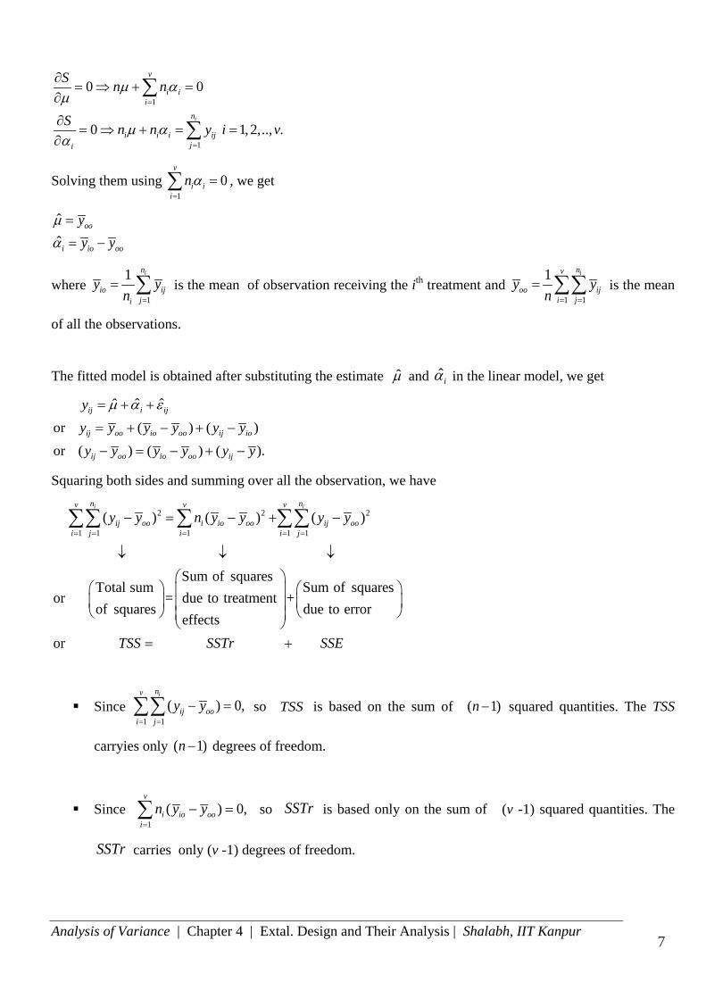
The fitted model is obtained after substituting the estimate µ̂ and ˆiα in the linear model, we get
ˆ ˆˆ
or ( ) ( )or ( ) ( ) ( ).
ij i ij
ij oo io oo ij io
ij oo io oo ij
yy y y y y yy y y y y y
µ α ε= + +
= + − + −
− = − + −
Squaring both sides and summing over all the observation, we have
2 2 2
1 1 1 1 1 ( ) ( ) ( )
Sum of squares
Total sumor = due to treatment
of squareseffects
i in nv v v
ij oo i io oo ij ooi j i i j
y y n y y y y= = = = =
− = − + −
↓ ↓ ↓
∑∑ ∑ ∑∑
Sum of squares+
due to error
or TSS SSTr SSE
= +
Since 1 1
( ) 0,inv
ij ooi j
y y= =
− =∑∑ so TSS is based on the sum of ( 1)n − squared quantities. The TSS
carryies only ( 1)n − degrees of freedom.
Since 1
( ) 0,=
− =∑v
i io ooi
n y y so SSTr is based only on the sum of (v -1) squared quantities. The
SSTr carries only (v -1) degrees of freedom.
Analysis of Variance | Chapter 4 | Extal. Design and Their Analysis | Shalabh, IIT Kanpur 8 8
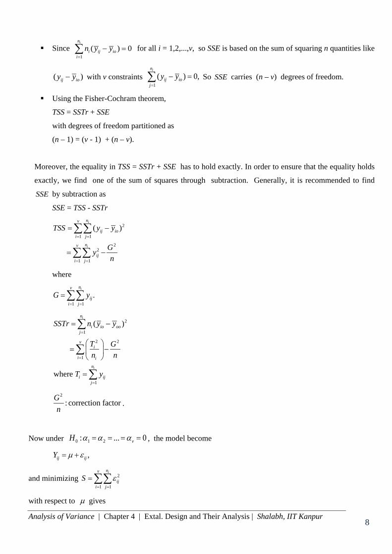
Since 1
( ) 0in
i ij ioi
n y y=
− =∑ for all i = 1,2,...,v, so SSE is based on the sum of squaring n quantities like
( )ij ioy y− with v constraints 1( ) 0,
=
− =∑in
ij ioj
y y So SSE carries (n – v) degrees of freedom.
Using the Fisher-Cochram theorem,
TSS = SSTr + SSE with degrees of freedom partitioned as
(n – 1) = (v - 1) + (n – v).
Moreover, the equality in TSS = SSTr + SSE has to hold exactly. In order to ensure that the equality holds
exactly, we find one of the sum of squares through subtraction. Generally, it is recommended to find
SSE by subtraction as SSE = TSS - SSTr
2
1 1
22
1 1
( )i
i
nv
ij ioi j
nv
iji j
TSS y y
Gyn
= =
= =
= −
= −
∑∑
∑∑
where
1 1.
inv
iji j
G y= =
=∑∑
2
1
2 2
1
1
( )
where
i
i
n
i io ooj
vi
i i
n
i ijj
SSTr n y y
T Gn n
T y
=
=
=
= −
= −
=
∑
∑
∑
2
: correction factorGn
.
Now under 0 1 2: ... 0α α α= = = =vH , the model become
,ij ijY µ ε= +
and minimizing 2
1 1
inv
iji j
S ε= =
=∑∑
with respect to µ gives
Analysis of Variance | Chapter 4 | Extal. Design and Their Analysis | Shalabh, IIT Kanpur 9 9
ˆ0 .ooS G y
nµ
µ∂
= ⇒ = =∂
The SSE under 0H becomes
2
1 1( )
inv
ij ooi j
SSE y y= =
= −∑∑
and thus .TSS SSE=
This TSS under 0H contains the variation only due to the random error whereas the earlier
TSS SSTr SSE= + contains the variation due to treatments and errors both. The difference between the two
will provides the effect of treatments in terms of sum of squares as
2
1( )
v
i i ooi
SSTr n y y=
= −∑ .
• Expectations
2
1 1
2
1 1
2 2.
1 1 1
22
1
2
2
( ) ( )
( )
( ) ( )
( )
( )
i
i
i
nv
ij ioi j
nv
ij ioi j
nv v
ij i ioi j i
v
ii i
E SSE E y y
E n E
n nn
n vSSEE MSE En v
ε ε
ε ε
σσ
σ
σ
= =
= =
= = =
=
= −
= −
= −
= −
= −
= = −
∑∑
∑∑
∑∑ ∑
∑
2
1
2
1
2 2 2
1 1
2 22
1 1
2 2
1
2 2
1
( ) ( )
( )
( 1)
1( ) .1 1
v
i io ooi
v
i i io ooi
v v
i i i io ooi i
v v
i i ii i i
v
i ii
v
i ii
E SSTr n E y y
n E
n n n
n n nn n
n v
SStrE MSTr E nv v
α ε ε
α ε ε
σ σα
α σ
α σ
=
=
= =
= =
=
=
= −
= + −
= + −
= + −
= + −
= = + − −
∑
∑
∑ ∑
∑ ∑
∑
∑
Analysis of Variance | Chapter 4 | Extal. Design and Their Analysis | Shalabh, IIT Kanpur 10 10
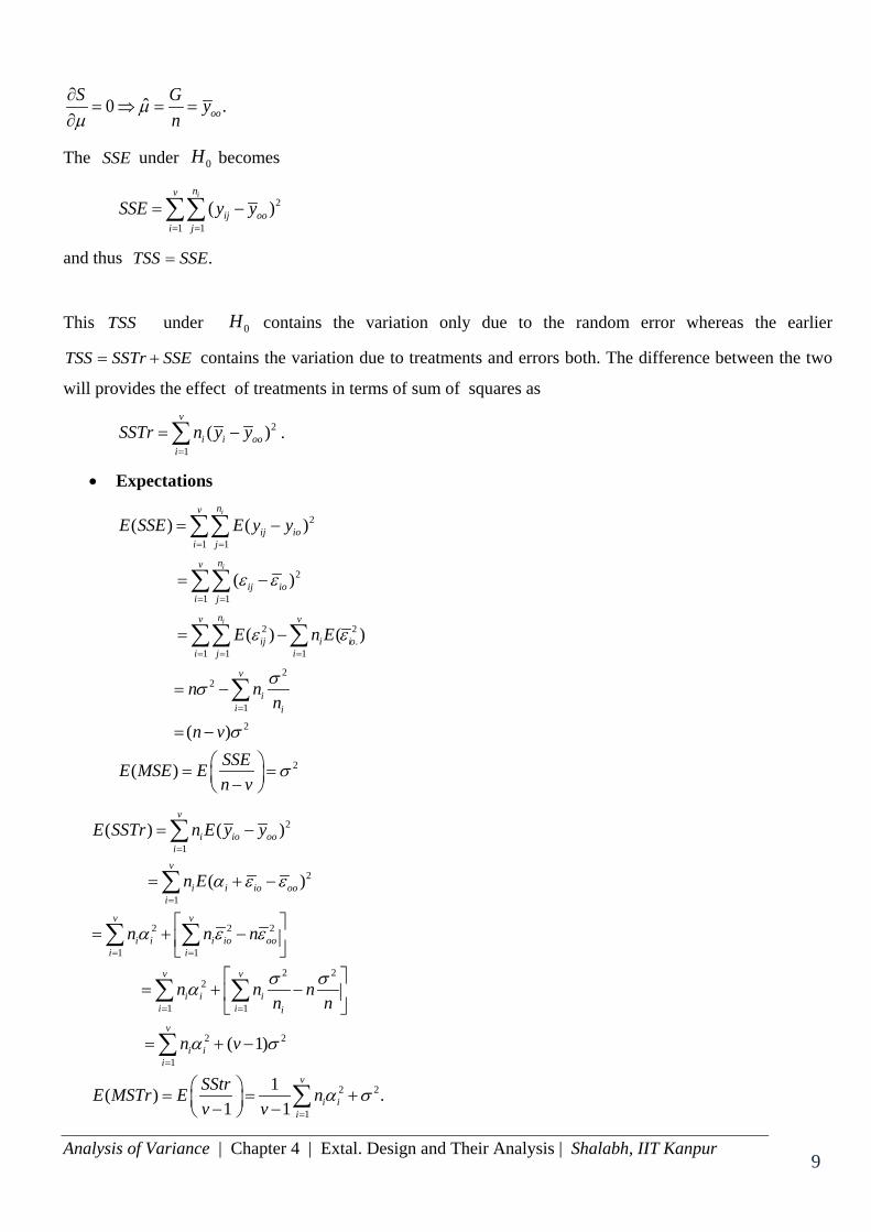
In general ( ) 2E MSTr σ≠ but under 0 ,H all 0iα = and so
2( )E MSTr σ= .
Distributions and decision rules:
Using the normal distribution property of ' ,ε ij s we find that 'ijy s are also normal as they are the linear
combination of ' .ij sε
202
202
0
0 *; 1, .
~ ( 1) under
~ ( ) under
and are independently distributed
~ ( 1, ) under .
Reject at * level of significance if v n v
SSTr v H
SSE n v H
SSTr SSEMStr F v n v HMSE
H F Fα
χσ
χσ
α − −
− −
− −
−
− − −
− >
[Note: We denote the level of significance here by *α because α has been used for denoting the factor]
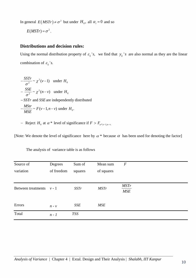
The analysis of variance table is as follows
Source of Degrees Sum of Mean sum F
variation of freedom squares of squares
Between treatments v - 1 SSTr MSTr MSTrMSE
Errors n - v SSE MSE
Total n - 1 TSS
Analysis of Variance | Chapter 4 | Extal. Design and Their Analysis | Shalabh, IIT Kanpur 11 11
Randomized Block Design
If large number of treatments are to be compared, then large number of experimental units are required. This
will increase the variation among the responses and CRD may not be appropriate to use. In such a case
when the experimental material is not homogeneous and there are v treatments to be compared, then it may
be possible to
• group the experimental material into blocks of sizes v units.
• Blocks are constructed such that the experimental units within a block are relatively homogeneous
and resemble to each other more closely than the units in the different blocks.
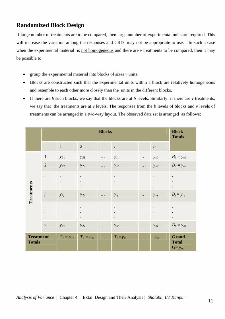
• If there are b such blocks, we say that the blocks are at b levels. Similarly if there are v treatments,
we say that the treatments are at v levels. The responses from the b levels of blocks and v levels of
treatments can be arranged in a two-way layout. The observed data set is arranged as follows:
Blocks Block Totals
1 2 i b
Tre
atm
ents
1 y11 y21 … yi1 … yb1 B1 = yo1
2 y12 y22 … yi2 … yb2 B2 = yo2
.
.
.
.
.
.
.
.
.
. . .
. . .
.
.
.
j y1j y2j … yij … ybj Bj = yoj
.
.
.
. . .
. . .
. . .
.
.
.
v y1v y2v … yiv … ybv Bb = yob
Treatment Totals
T1 = y1o T2 =y2o … Ti =yio … yvo Grand Total G= yoo
Analysis of Variance | Chapter 4 | Extal. Design and Their Analysis | Shalabh, IIT Kanpur 12 12
Layout: A two-way layout is called a randomized block design (RBD) or a randomized complete block design (RCB)
if within each block, the v treatments are randomly assigned to v experimental units such that each of the v!
ways of assigning the treatments to the units has the same probability of being adopted in the experiment
and the assignment in different blocks are statistically independent.
The RBD utilizes the principles of design - randomization, replication and local control - in the following
way:
1. Randomization: - Number the v treatments 1,2,…,v.
- Number the units in each block as 1, 2,...,v.
- Randomly allocate the v treatments to v experimental units in each block.
2. Replication Since each treatment is appearing in the each block, so every treatment will appear in all the blocks. So
each treatment can be considered as if replicated the number of times as the number of blocks. Thus in
RBD, the number of blocks and the number of replications are same.
3. Local control Local control is adopted in RBD in following way:
- First form the homogeneous blocks of the xperimental units.
- Then allocate each treatment randomly in each block.
The error variance now will be smaller because of homogeneous blocks and some variance will be parted
away from the error variance due to the difference among the blocks.

Analysis of Variance | Chapter 4 | Extal. Design and Their Analysis | Shalabh, IIT Kanpur 13 13
Example:
Suppose there are 7 treatment denoted as 1 2 7, ,..,T T T corresponding to 7 levels of a factor to be included in 4
blocks. So one possible layout of the assignment of 7 treatments to 4 different blocks in a RBD is as
follows
Analysis Let
:ijy Individual measurements of jth treatment in ith block, i = 1,2,...,b, j = 1,2,...,v.
ijy ’s are independently distributed following 2( , )i jN µ β τ σ+ +
where :µ overall mean effect
iβ : ith block effect
jτ : jth treatment effect
such that 1 1
0, 0b v
i ji jβ τ
= =
= =∑ ∑ .
There are two null hypotheses to be tested.
- related to the block effects
0 1 2: .... 0.B bH β β β= = = =
- related to the treatment effects
0 1 2: .... 0.T vH τ τ τ= = = =
The linear model in this case is a two-way model as
, 1, 2,.., ; 1, 2,..,ij i j ijy i b j vµ β τ ε= + + + = =
where ijε are identically and independently distributed random errors following a normal distribution with
mean 0 and variance 2σ .
Block 1 2T 7T 3T 5T 1T 4T 6T
Block 2 1T 6T 7T 4T 5T 3T 2T
Block 3 7T 5T 1T 6T 4T 2T 3T
Block 4 4T 1T 5T 6T 2T 7T 3T

Analysis of Variance | Chapter 4 | Extal. Design and Their Analysis | Shalabh, IIT Kanpur 14 14
The tests of hypothesis can be derived using the likelihood ratio test or the principle of least squares. The use
of likelihood ratio test has already been demonstrated earlier, so we now use the principle of least squares.
2 2
1 1 1 1Minimizing ( )
b v b v
ij ij i ji j i j
S yε µ β τ= = = =
= = − − −∑∑ ∑∑
and solving the normal equation
0, 0, 0 for all 1, 2,.., , 1, 2,.., .i j
S S S i b j vµ β τ∂ ∂ ∂
= = = = =∂ ∂ ∂
the least squares estimators are obtained as
ˆ ,ˆ ,ˆ .
oo
i io oo
j oj oo
y
y yy y
µ
βτ
=
= −= −
The fitted model is
ˆ ˆˆ ˆ
= ( ) ( ) ( ).µ β τ ε= + + +
+ − + − + − − +ij i j ij
oo io oo oj oo ij io oj oo
yy y y y y y y y y
Squaring both sides and summing over i and j gives
2 2 2 2
1 1 1 1 1 1( ) ( ) ( ) ( )
or
b v b v b v
ij oo io oo oj oo ij io oj ooi j i j i j
y y v y y b y y y y y y
TSS SSBl SSTr SSE= = = = = =
− = − + − + − − +
= + +
∑∑ ∑ ∑ ∑∑
with degrees of freedom partitioned as
1 ( 1) ( 1) ( 1)( 1).bv b v b v− = − + − + − −
The reason for the number of degrees of freedom for different sums of squares is the same as in the case of
CRD.
2
1 1
22
1 1
Here ( )b v
ij ooi j
b v
iji j
TSS y y
Gybv
= =
= =
= −
= −
∑∑
∑∑
2
:Gbv
correction factor.
1 1
b v
iji j
G y= =
=∑∑ : Grand total of all the observation.
Analysis of Variance | Chapter 4 | Extal. Design and Their Analysis | Shalabh, IIT Kanpur 15 15
2
12 2
1
1
( )
: block total
n
io ooi
bi
iv
thi ij
j
SSBl v y y
B Gb bv
B y i
=
=
=
= −
= −
=
∑
∑
∑
2
1
2 2
1
( )v
oj ooj
vj
j
SSTr b y y
T Gv bv
=
=
= −
= −
∑
∑
1
2
1 1
: treatment total
( ) .
bth
j iji
b v
ij io oj ooi j
T y j
SSE y y y y
=
= =
=
= − − +
∑
∑∑
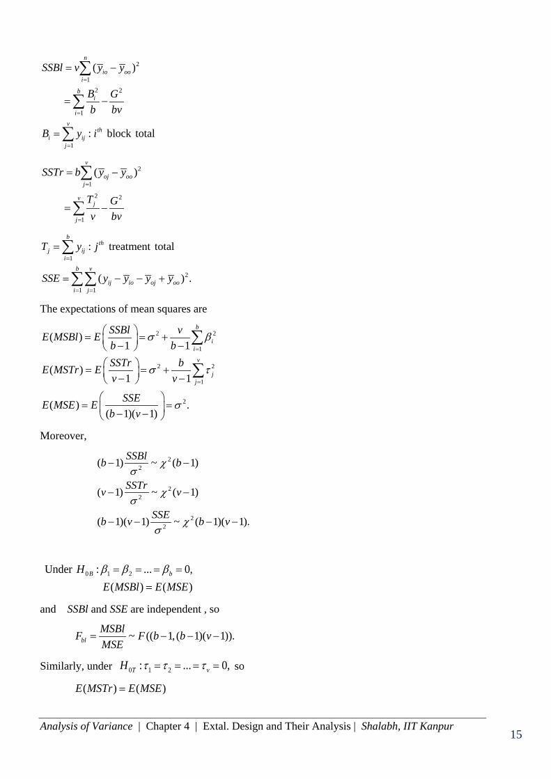
The expectations of mean squares are
2 2
1
2 2
1
2
( )1 1
( )1 1
( ) .( 1)( 1)
b
ii
v
jj
SSBl vE MSBl Eb bSSTr bE MSTr Ev v
SSEE MSE Eb v
σ β
σ τ
σ
=
=
= = + − − = = + − −
= = − −
∑
∑
Moreover,
22
22
22
( 1) ~ ( 1)
( 1) ~ ( 1)
( 1)( 1) ~ ( 1)( 1).
SSBlb b
SSTrv v
SSEb v b v
χσ
χσ
χσ
− −
− −
− − − −
0 1 2Under : ... 0,( ) ( )
B bHE MSBl E MSEβ β β= = = =
=
and SSBl and SSE are independent , so
~ (( 1, ( 1)( 1)).blMSBlF F b b vMSE
= − − −
Similarly, under 0 1 2: ... 0,T vH τ τ τ= = = = so
( ) ( )E MSTr E MSE=
Analysis of Variance | Chapter 4 | Extal. Design and Their Analysis | Shalabh, IIT Kanpur 16 16
and SSTr and SSE are independent , so
~ ( 1), ( 1)( 1)).TrMSTrF F v b vMSE
= − − −
Reject 0 (( 1), ( 1)( 1)B beH if F F b b vα> − − −
Reject 0 (( 1), ( 1)( 1))T TrH if F F v b vα> − − −
If 0BH is accepted, then it indicates that the blocking is not necessary for future experimentation.
If 0TH is rejected then it indicates that the treatments are different. Then the multiple comparison tests are
used to divide the entire set of treatments into different subgroup such that the treatments in the same
subgroup have the same treatment effect and those in the different subgroups have different treatment
effects.
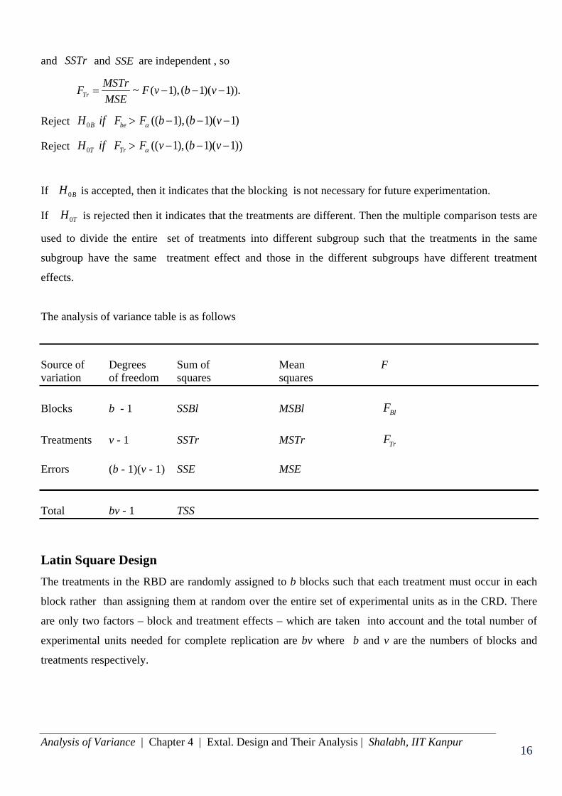
The analysis of variance table is as follows
Source of Degrees Sum of Mean F variation of freedom squares squares Blocks b - 1 SSBl MSBl BlF Treatments v - 1 SSTr MSTr TrF Errors (b - 1)(v - 1) SSE MSE Total bv - 1 TSS
Latin Square Design The treatments in the RBD are randomly assigned to b blocks such that each treatment must occur in each
block rather than assigning them at random over the entire set of experimental units as in the CRD. There
are only two factors – block and treatment effects – which are taken into account and the total number of
experimental units needed for complete replication are bv where b and v are the numbers of blocks and
treatments respectively.
Analysis of Variance | Chapter 4 | Extal. Design and Their Analysis | Shalabh, IIT Kanpur 17 17
If there are three factors and suppose there are b, v and k levels of each factor, then the total number of
experimental units needed for a complete replication are bvk. This increases the cost of experimentation and
the required number of experimental units over RBD.
In Latin square design (LSD), the experimental material is divided into rows and columns, each having the
same number of experimental units which is equal to the number of treatments. The treatments are allocated
to the rows and the columns such that each treatment occurs once and only once in the each row and in the
each column.
In order to allocate the treatment to the experimental units in rows and columns, we take the help from Latin
squares.
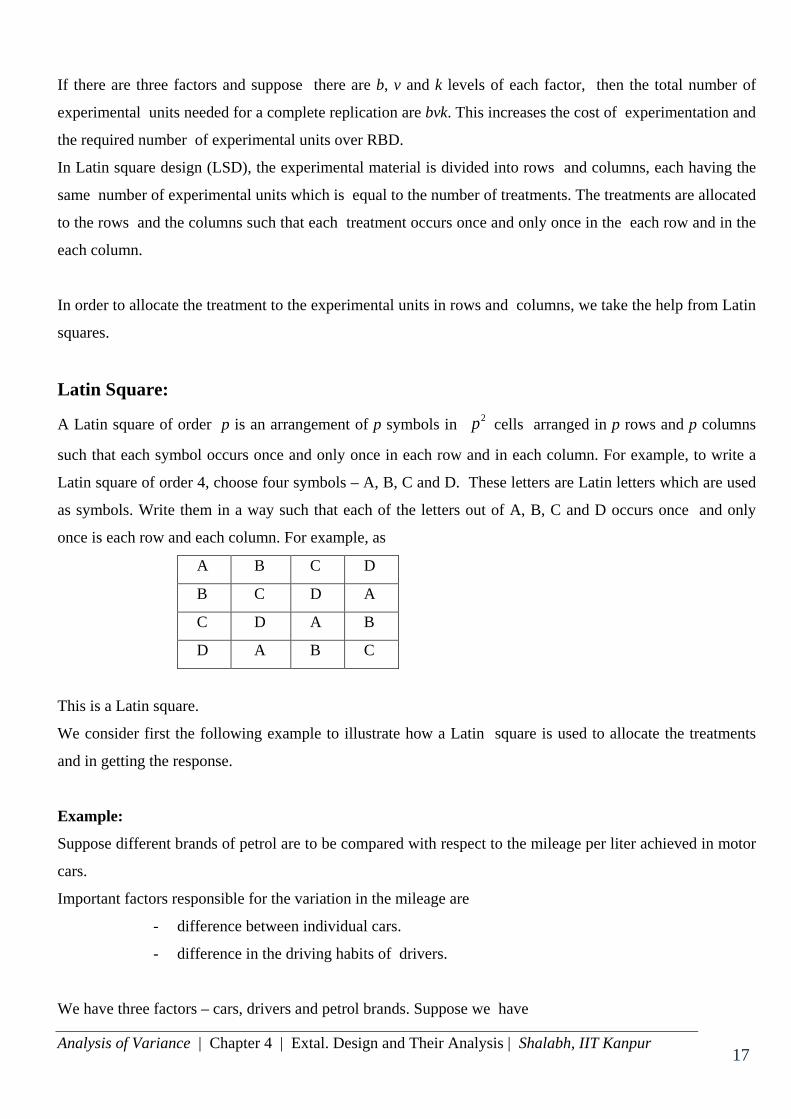
Latin Square:
A Latin square of order p is an arrangement of p symbols in 2p cells arranged in p rows and p columns
such that each symbol occurs once and only once in each row and in each column. For example, to write a
Latin square of order 4, choose four symbols – A, B, C and D. These letters are Latin letters which are used
as symbols. Write them in a way such that each of the letters out of A, B, C and D occurs once and only
once is each row and each column. For example, as
A B C D
B C D A
C D A B
D A B C
This is a Latin square.
We consider first the following example to illustrate how a Latin square is used to allocate the treatments
and in getting the response.
Example:
Suppose different brands of petrol are to be compared with respect to the mileage per liter achieved in motor
cars.
Important factors responsible for the variation in the mileage are
- difference between individual cars.
- difference in the driving habits of drivers.
We have three factors – cars, drivers and petrol brands. Suppose we have
Analysis of Variance | Chapter 4 | Extal. Design and Their Analysis | Shalabh, IIT Kanpur 18 18
- 4 types of cars denoted as 1, 2, 3, 4.
- 4 drivers that are represented by as a, b, c, d.
- 4 brands of petrol are indicated by as A, B, C, D.
Now the complete replication will require 4 4 4 64× × = number of experiments. We choose only 16
experiments. To choose such 16 experiments, we take the help of Latin square. Suppose we choose the
following Latin square:
A B C D
B C D A
C D A B
D A B C
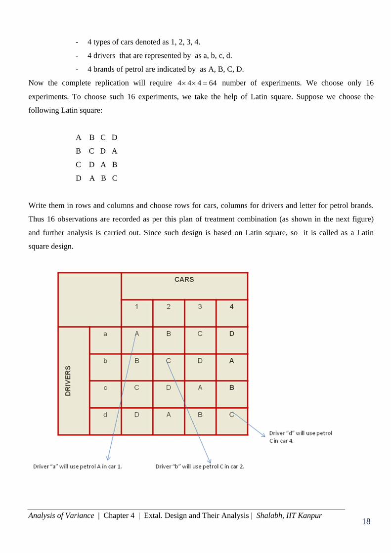
Write them in rows and columns and choose rows for cars, columns for drivers and letter for petrol brands.
Thus 16 observations are recorded as per this plan of treatment combination (as shown in the next figure)
and further analysis is carried out. Since such design is based on Latin square, so it is called as a Latin
square design.
Analysis of Variance | Chapter 4 | Extal. Design and Their Analysis | Shalabh, IIT Kanpur 19 19
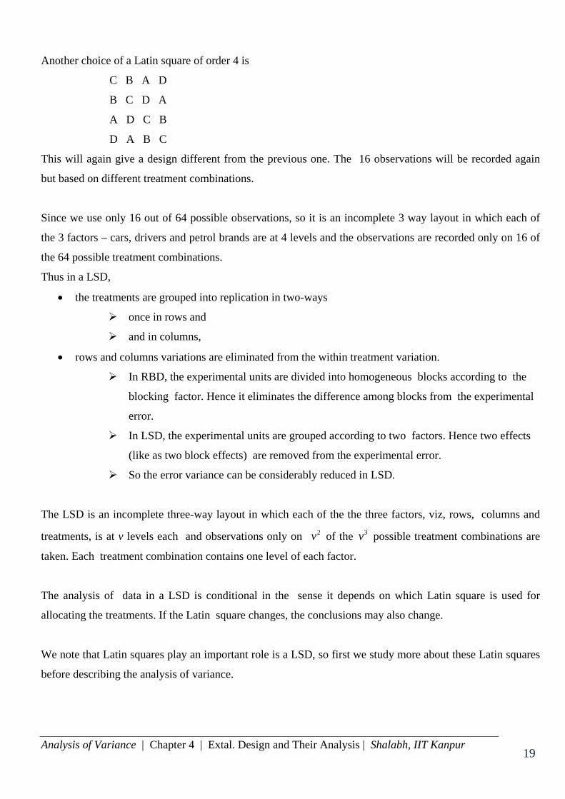
Another choice of a Latin square of order 4 is
C B A D
B C D A
A D C B
D A B C
This will again give a design different from the previous one. The 16 observations will be recorded again
but based on different treatment combinations.
Since we use only 16 out of 64 possible observations, so it is an incomplete 3 way layout in which each of
the 3 factors – cars, drivers and petrol brands are at 4 levels and the observations are recorded only on 16 of
the 64 possible treatment combinations.
Thus in a LSD,
• the treatments are grouped into replication in two-ways
once in rows and
and in columns,
• rows and columns variations are eliminated from the within treatment variation.
In RBD, the experimental units are divided into homogeneous blocks according to the
blocking factor. Hence it eliminates the difference among blocks from the experimental
error.
In LSD, the experimental units are grouped according to two factors. Hence two effects
(like as two block effects) are removed from the experimental error.
So the error variance can be considerably reduced in LSD.
The LSD is an incomplete three-way layout in which each of the the three factors, viz, rows, columns and
treatments, is at v levels each and observations only on 2v of the 3v possible treatment combinations are
taken. Each treatment combination contains one level of each factor.
The analysis of data in a LSD is conditional in the sense it depends on which Latin square is used for
allocating the treatments. If the Latin square changes, the conclusions may also change.
We note that Latin squares play an important role is a LSD, so first we study more about these Latin squares
before describing the analysis of variance.
Analysis of Variance | Chapter 4 | Extal. Design and Their Analysis | Shalabh, IIT Kanpur 20 20
Standard form of Latin square
A Latin square is in the standard form if the symbols in the first row and first columns are in the natural
order (Natural order means the order of alphabets like A, B, C, D,…).
Given a Latin square, it is possible to rearrange the columns so that the first row and first column remain in
natural order.
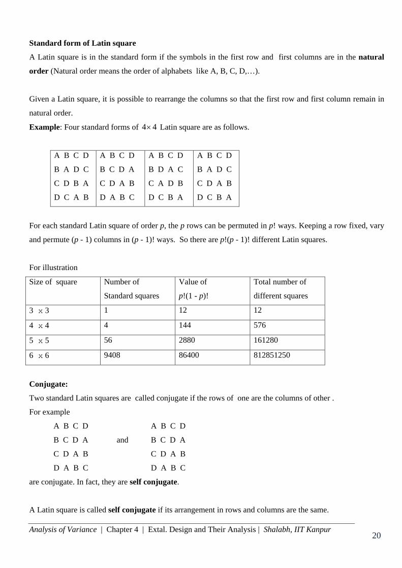
Example: Four standard forms of 4 4× Latin square are as follows.
A B C D
B A D C
C D B A
D C A B
A B C D
B C D A
C D A B
D A B C
A B C D
B D A C
C A D B
D C B A
A B C D
B A D C
C D A B
D C B A
For each standard Latin square of order p, the p rows can be permuted in p! ways. Keeping a row fixed, vary
and permute (p - 1) columns in (p - 1)! ways. So there are p!(p - 1)! different Latin squares.
For illustration
Size of square Number of
Standard squares
Value of
p!(1 - p)!
Total number of
different squares
3 x 3 1 12 12
4 x 4 4 144 576
5 x 5 56 2880 161280
6 x 6 9408 86400 812851250
Conjugate:
Two standard Latin squares are called conjugate if the rows of one are the columns of other .
For example
A B C D A B C D
B C D A and B C D A
C D A B C D A B
D A B C D A B C
are conjugate. In fact, they are self conjugate.
A Latin square is called self conjugate if its arrangement in rows and columns are the same.
Analysis of Variance | Chapter 4 | Extal. Design and Their Analysis | Shalabh, IIT Kanpur 21 21
Transformation set:
A set of all Latin squares obtained from a single Latin square by permuting its rows, columns and symbols
is called a transformation set.
From a Latin square of order p, p!(p - 1)! different Latin squares can be obtained by making p! permutations
of columns and (p - 1)! permutations of rows which leaves the first row in place. Thus
Number of different p!(p - 1)! X number of standard Latin
Latin squares of order = squares in the set
p in a transformation set
Orthogonal Latin squares
If two Latin squares of the same order but with different symbols are such that when they are superimposed
on each other, every ordered pair of symbols (different) occurs exactly once in the Latin square, then they
are called orthogonal.
Greco-Latin square:
A pair of orthogonal Latin squares, one with Latin symbols and the other with Greek symbols forms a
Greco-Latin square.
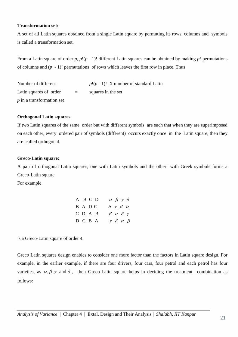
For example
A B C D B A D C C D A B D C B A
α β γ δδ γ β αβ α δ γγ δ α β
is a Greco-Latin square of order 4.
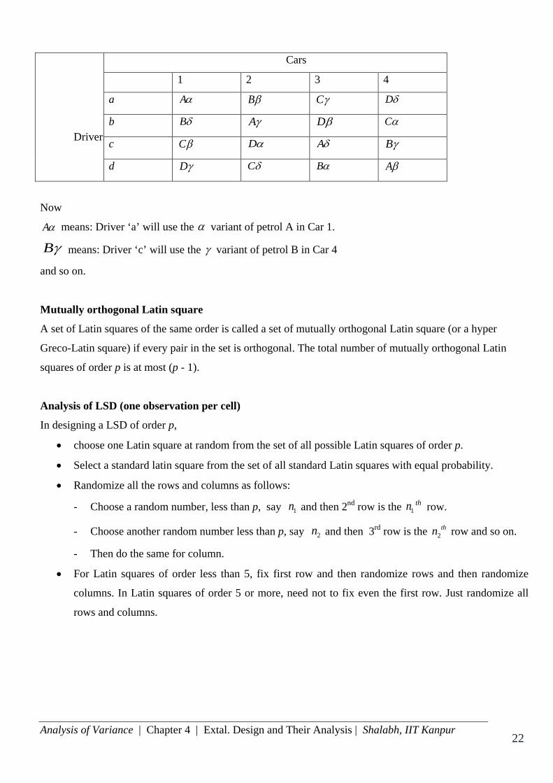
Greco Latin squares design enables to consider one more factor than the factors in Latin square design. For
example, in the earlier example, if there are four drivers, four cars, four petrol and each petrol has four
varieties, as , , andα β γ δ , then Greco-Latin square helps in deciding the treatment combination as
follows:
Analysis of Variance | Chapter 4 | Extal. Design and Their Analysis | Shalabh, IIT Kanpur 22 22
Drivers
Cars
1 2 3 4
a Aα Bβ Cγ Dδ
b Bδ Aγ Dβ Cα
c Cβ Dα Aδ Bγ
d Dγ Cδ Bα Aβ
Now
Aα means: Driver ‘a’ will use the α variant of petrol A in Car 1.
Bγ means: Driver ‘c’ will use the γ variant of petrol B in Car 4
and so on.
Mutually orthogonal Latin square
A set of Latin squares of the same order is called a set of mutually orthogonal Latin square (or a hyper
Greco-Latin square) if every pair in the set is orthogonal. The total number of mutually orthogonal Latin
squares of order p is at most (p - 1).
Analysis of LSD (one observation per cell)
In designing a LSD of order p,
• choose one Latin square at random from the set of all possible Latin squares of order p.
• Select a standard latin square from the set of all standard Latin squares with equal probability.
• Randomize all the rows and columns as follows:
- Choose a random number, less than p, say 1n and then 2nd row is the 1n th row.
- Choose another random number less than p, say 2n and then 3rd row is the 2thn row and so on.
- Then do the same for column.
• For Latin squares of order less than 5, fix first row and then randomize rows and then randomize
columns. In Latin squares of order 5 or more, need not to fix even the first row. Just randomize all
rows and columns.
Analysis of Variance | Chapter 4 | Extal. Design and Their Analysis | Shalabh, IIT Kanpur 23 23
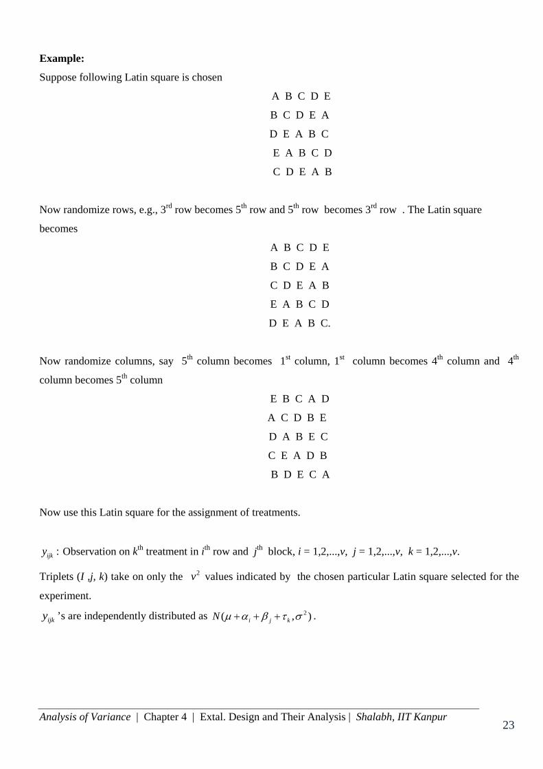
Example:
Suppose following Latin square is chosen
A B C D E
B C D E A
D E A B C
E A B C D
C D E A B
Now randomize rows, e.g., 3rd row becomes 5th row and 5th row becomes 3rd row . The Latin square
becomes
A B C D E
B C D E A
C D E A B
E A B C D
D E A B C.
Now randomize columns, say 5th column becomes 1st column, 1st column becomes 4th column and 4th
column becomes 5th column
E B C A D
A C D B E
D A B E C
C E A D B
B D E C A
Now use this Latin square for the assignment of treatments.
:ijky Observation on kth treatment in ith row and jth block, i = 1,2,...,v, j = 1,2,...,v, k = 1,2,...,v.
Triplets (I ,j, k) take on only the 2v values indicated by the chosen particular Latin square selected for the
experiment.
ijky ’s are independently distributed as 2( , )i j kN µ α β τ σ+ + + .
Analysis of Variance | Chapter 4 | Extal. Design and Their Analysis | Shalabh, IIT Kanpur 24 24
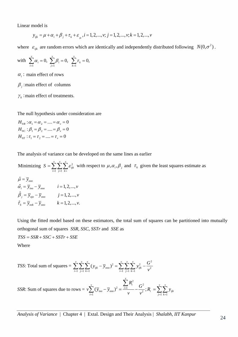
Linear model is
, 1, 2,..., ; 1, 2,..., ; 1, 2,...,ijkijk i j ky i v j v k vµ α β τ ε= + + + + = = =
where ijkε are random errors which are identically and independently distributed following 2(0, )N σ .
with 1 1 1
0, 0, 0,v v v
i i ki j kα β τ
= = =
= = =∑ ∑ ∑
:iα main effect of rows
:jβ main effect of columns
:kγ main effect of treatments.
The null hypothesis under consideration are
0 1 2
0 1 2
0 1 2
: .... 0: .... 0: .... 0
α α αβ β βτ τ τ
= = = == = = == = = =
R v
C v
T v
HHH
The analysis of variance can be developed on the same lines as earlier
2
1 1Minimizing
v v v
ijki j k
S ε= = =
=∑∑∑ with respect to , ,i jµ α β and kτ given the least squares estimate as
ˆ ˆ 1, 2,...,ˆ 1, 2,...,ˆ 1, 2,..., .
ooo
i ioo ooo
j ojo ooo
k ook ooo
yy y i v
y y j vy y k v
µα
β
τ
== − =
= − =
= − =
Using the fitted model based on these estimators, the total sum of squares can be partitioned into mutually
orthogonal sum of squares SSR, SSC, SSTr and SSE as
TSS SSR SSC SSTr SSE= + + +
Where
TSS: Total sum of squares = 2
2 22
1 1 1 1 1 1( )
v v v v v v
ijk ooo ijki j k i j k
Gy y yv= = = = = =
− = −∑∑∑ ∑∑∑
SSR: Sum of squares due to rows =
22
2 12
1 1 1( ) ;
v
iv v vi
ioo ooo i ijki j k
RGv y y R y
v v=
= = =
− = − =∑
∑ ∑∑
Analysis of Variance | Chapter 4 | Extal. Design and Their Analysis | Shalabh, IIT Kanpur 25 25
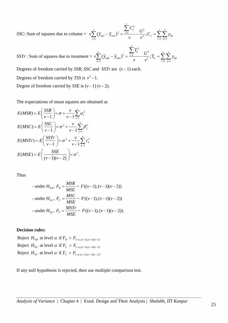
SSC: Sum of squares due to column =
22
2 12
1 1 1( ) ;
v
jv v vi
ojo ooo j ijkj i k
CGv y y C y
v v=
= = =
− = − =∑
∑ ∑∑
SSTr : Sum of squares due to treatment =
22
2 12
1 1 1( ) ;
v
kv v vi
ook ooo k ijkk i j
TGv y y T y
v v=
= = =
− = − =∑
∑ ∑∑
Degrees of freedom carried by SSR, SSC and SSTr are (v - 1) each.
Degrees of freedom carried by TSS is 2 1.v −
Degree of freedom carried by SSE is (v - 1) (v - 2).
The expectations of mean squares are obtained as
2
1
2 2
1
2 2
1
2
( )1 1
( )1 1
( )1 1
( ) .( 1)( 2)
σ α
σ β
σ τ
σ
=
=
=
= = + − − = = + − −
= = + − −
= = − −
∑
∑
∑
v
ii
v
jj
v
kk
SSR vE MSR Ev vSSC vE MSC Ev vSSTr vE MSTr Ev v
SSEE MSE Ev v
Thus
0
0
0
- under , ~ (( 1), ( 1)( 2))
- under , ~ (( 1), ( 1)( 2))
- under , ~ (( 1), ( 1)( 2)).
= − − −
= − − −
= − − −
R R
C C
T T
MSRH F F v v vMSEMSCH F F v v vMSEMSTrH F F v v vMSE
Decision rules:
0 1 ; ( 1),( 1)( 2)
0 1 ;( 1),( 1)( 2)
0 1 ;( 1),( 1)( 2)
Reject at level if Reject at level if Reject at level if .
R R v v v
C C v v v
T T v v v
H F FH F FH F F
α
α
α
α
α
α
− − − −
− − − −
− − − −
>
>
>
If any null hypothesis is rejected, then use multiple comparison test.
Analysis of Variance | Chapter 4 | Extal. Design and Their Analysis | Shalabh, IIT Kanpur 26 26
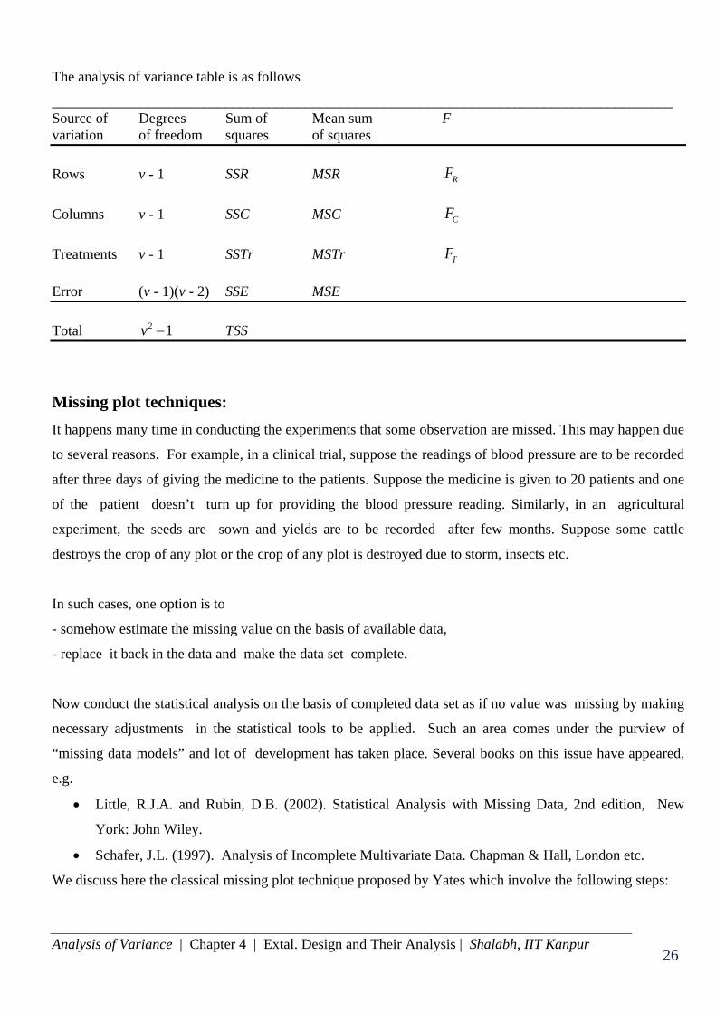
The analysis of variance table is as follows
______________________________________________________________________________________ Source of Degrees Sum of Mean sum F variation of freedom squares of squares Rows v - 1 SSR MSR RF Columns v - 1 SSC MSC CF Treatments v - 1 SSTr MSTr TF Error (v - 1)(v - 2) SSE MSE Total 2 1v − TSS
Missing plot techniques: It happens many time in conducting the experiments that some observation are missed. This may happen due
to several reasons. For example, in a clinical trial, suppose the readings of blood pressure are to be recorded
after three days of giving the medicine to the patients. Suppose the medicine is given to 20 patients and one
of the patient doesn’t turn up for providing the blood pressure reading. Similarly, in an agricultural
experiment, the seeds are sown and yields are to be recorded after few months. Suppose some cattle
destroys the crop of any plot or the crop of any plot is destroyed due to storm, insects etc.
In such cases, one option is to
- somehow estimate the missing value on the basis of available data,
- replace it back in the data and make the data set complete.
Now conduct the statistical analysis on the basis of completed data set as if no value was missing by making
necessary adjustments in the statistical tools to be applied. Such an area comes under the purview of
“missing data models” and lot of development has taken place. Several books on this issue have appeared,
e.g.
• Little, R.J.A. and Rubin, D.B. (2002). Statistical Analysis with Missing Data, 2nd edition, New
York: John Wiley.
• Schafer, J.L. (1997). Analysis of Incomplete Multivariate Data. Chapman & Hall, London etc.
We discuss here the classical missing plot technique proposed by Yates which involve the following steps:

Analysis of Variance | Chapter 4 | Extal. Design and Their Analysis | Shalabh, IIT Kanpur 27 27
• Estimate the missing observations by the values which makes the error sum of squares to be
minimum.
• Substitute the unknown values by the missing observations.
• Express the error sum of squares as a function of these unknown values.
• Minimize the error sum of squares using principle of maxima/minima, i.e., differentiating it with
respect to the missing value and put it to zero and form a linear equation.
• Form as many linear equation as the number of unknown values (i.e., differentiate error sum of
squares with respect to each unknown value).
• Solve all the linear equations simultaneously and solutions will provide the missing values.
• Impute the missing values with the estimated values and complete the data.
• Apply analysis of variance tools.
• The error sum of squares thus obtained is corrected but treatment sum of squares are not corrected.
• The number of degrees of freedom associated with the total sum of squares are subtracted by the
number of missing values and adjusted in the error sum of squares. No change in the degrees of
freedom of sum of squares due to treatment is needed.
Analysis of Variance | Chapter 4 | Extal. Design and Their Analysis | Shalabh, IIT Kanpur 28 28
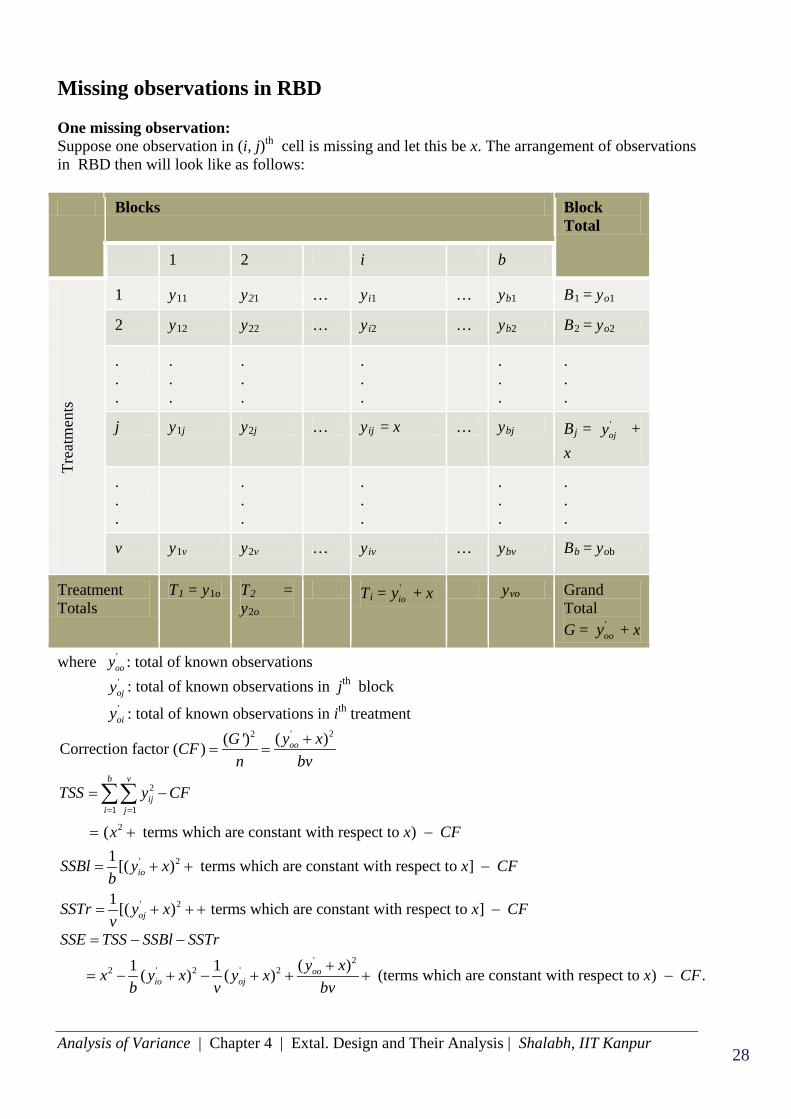
Missing observations in RBD One missing observation: Suppose one observation in (i, j)th cell is missing and let this be x. The arrangement of observations in RBD then will look like as follows: Blocks Block
Total
1 2 i b
Trea
tmen
ts
1 y11 y21 … yi1 … yb1 B1 = yo1
2 y12 y22 … yi2 … yb2 B2 = yo2
.
.
.
.
.
.
.
.
.
. . .
. . .
.
.
.
j y1j y2j … yij = x … ybj Bj = 'ojy +
x
.
.
.
. . .
. . .
. . .
.
.
.
v y1v y2v … yiv … ybv Bb = yob
Treatment Totals
T1 = y1o T2 = y2o
Ti = 'ioy + x yvo Grand
Total G = '
ooy + x
where 'ooy : total of known observations
'ojy : total of known observations in jth block
'oiy : total of known observations in ith treatment
' 22
2
1 1
2
' 2
( )( ')Correction factor ( )
( terms which are constant with respect to ) 1 [( ) terms which are constant with respect to ]
1 [(
oo
b v
iji j
io
y xGCFn bv
TSS y CF
x x CF
SSBl y x x CFb
SSTrv
= =
+= =
= −
= + −
= + + −
=
∑∑
' 2) terms which are constant with respect to ] ojy x x CF+ + + −
' 22 ' 2 ' 2 ( )1 1( ) ( ) (terms which are constant with respect to ) .oo
io oj
SSE TSS SSBl SSTry xx y x y x x CF
b v bv
= − −
+= − + − + + + −
Analysis of Variance | Chapter 4 | Extal. Design and Their Analysis | Shalabh, IIT Kanpur 29 29
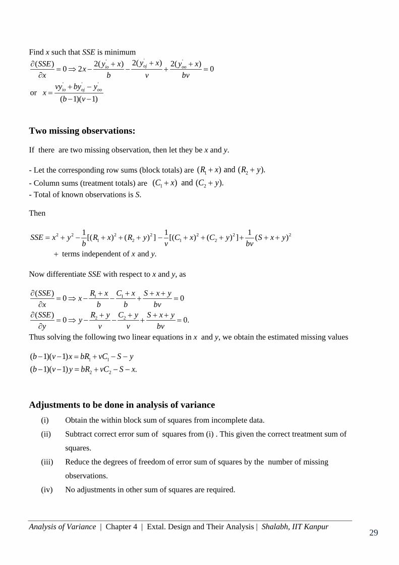
Find x such that SSE is minimum
'' '
' ' '
2( )2( ) 2( )( ) 0 2 0
or ( 1)( 1)
ojio oo
io oj oo
y xy x y xSSE xx b v bv
vy by yx
b v
++ +∂= ⇒ − − + =
∂+ −
=− −
Two missing observations: If there are two missing observation, then let they be x and y. - Let the corresponding row sums (block totals) are 1 2( ) and ( ).R x R y+ + - Column sums (treatment totals) are 1 2( ) and ( ).C x C y+ + - Total of known observations is S. Then
2 2 2 2 2 2 21 2 1 2
1 1 1[( ) ( ) ] [( ) ( ) ] ( )
terms independent of and .
= + − + + + − + + + + + +
+
SSE x y R x R y C x C y S x yb v bv
x y
Now differentiate SSE with respect to x and y, as
1 1
2 2
( ) 0 0
( ) 0 0.
R x C xSSE S x yxx b b bv
R y C ySSE S x yyy v v bv
+ +∂ + += ⇒ − − + =
∂+ +∂ + +
= ⇒ − − + =∂
Thus solving the following two linear equations in x and y, we obtain the estimated missing values
1 1
2 2
( 1)( 1)( 1)( 1) .b v x bR vC S yb v y bR vC S x− − = + − −− − = + − −
Adjustments to be done in analysis of variance (i) Obtain the within block sum of squares from incomplete data.
(ii) Subtract correct error sum of squares from (i) . This given the correct treatment sum of
squares.
(iii) Reduce the degrees of freedom of error sum of squares by the number of missing
observations.
(iv) No adjustments in other sum of squares are required.
Analysis of Variance | Chapter 4 | Extal. Design and Their Analysis | Shalabh, IIT Kanpur 30 30
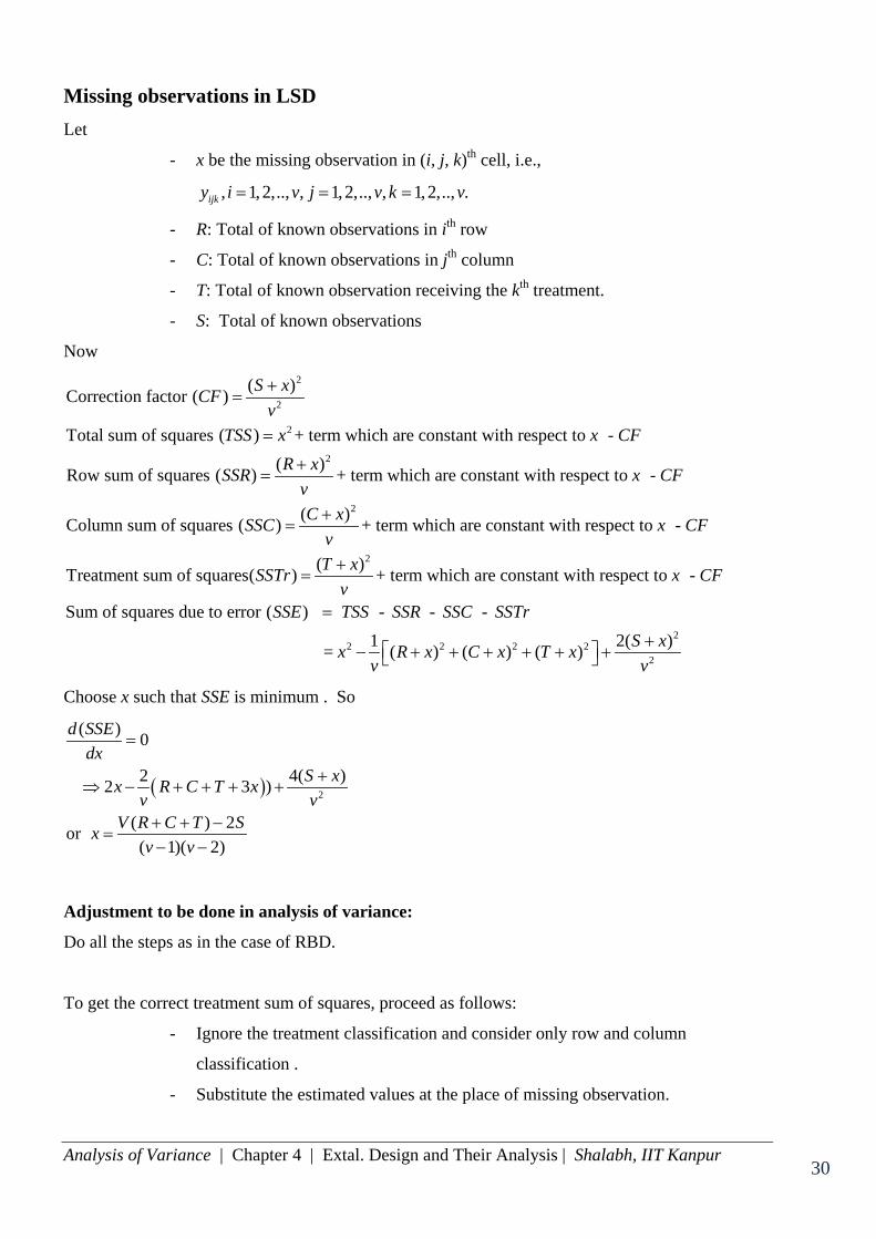
Missing observations in LSD Let
- x be the missing observation in (i, j, k)th cell, i.e.,
, 1, 2,.., , 1, 2,.., , 1, 2,.., .ijky i v j v k v= = =
- R: Total of known observations in ith row
- C: Total of known observations in jth column
- T: Total of known observation receiving the kth treatment.
- S: Total of known observations
Now 2
2
2
2
( )Correction factor ( )
Total sum of squares ( ) + term which are constant with respect to - ( )Row sum of squares ( ) + term which are constant with respect to -
Column sum
S xCFv
TSS x x CFR xSSR x CF
v
+=
=
+=
2
2
( ) of squares ( ) + term which are constant with respect to -
( )Treatment sum of squares( ) + term which are constant with respect to -
Sum of squares due to error ( )
C xSSC x CFvT xSSTr x CF
vSSE TS
+=
+=
=2
2 2 2 22
- - - 1 2( ) = ( ) ( ) ( )
S SSR SSC SSTrS xx R x C x T x
v v+ − + + + + + +
Choose x such that SSE is minimum . So
( ) 2
( ) 0
2 4( )2 3 )
( ) 2or( 1)( 2)
d SSEdx
S xx R C T xv v
V R C T Sxv v
=
+⇒ − + + + +
+ + −=
− −
Adjustment to be done in analysis of variance:
Do all the steps as in the case of RBD.
To get the correct treatment sum of squares, proceed as follows:
- Ignore the treatment classification and consider only row and column
classification .
- Substitute the estimated values at the place of missing observation.

Analysis of Variance | Chapter 4 | Extal. Design and Their Analysis | Shalabh, IIT Kanpur 31 31
- Obtain the error sum of squares from complete data, say SSE 1 .
- Let 2SSE be the error sum of squares based on LSD obtained earlier.
- Find corrected treatment sum of squares = 2 1SSE SSE− .
- Reduce of degrees of freedom of error sum of squares by the number of missing
values.