Experimental challenges of shear rheology: how to avoid ... · Experimental challenges of shear rheology: how to avoid bad data Randy H. Ewoldt, Michael T. Johnston, and Lucas M

Experimental challenges of shear rheology: howto avoid bad data

Randy H. Ewoldt, Michael T. Johnston, and Lucas M. Caretta

Abstract A variety of measurement artifacts can be blamed for misinterpretations ofshear-thinning, shear-thickening, and viscoelastic responses, when the material doesnot actually have these properties. The softness and activity of biological materialswill often magnify the challenges of experimental rheological measurements. Thetheoretical definitions of rheological material functions are based on stress, strain,and strain-rate components in simple deformation fields. In reality, one typicallymeasures loads and displacements at the boundaries of a sample, and the calcula-tion of true stress and strain may be encumbered by instrument resolution, instru-ment inertia, sample inertia, boundary effects, and volumetric effects. Here we dis-cuss these common challenges in measuring shear material functions in the contextof soft, water-based, and even living biological complex fluids. We discuss tech-niques for identifying and minimizing experimental errors and for pushing the ex-perimental limits of rotational shear rheometers. Two extreme case studies are used:an ultra-soft aqueous polymer/fiber network (hagfish defense gel), and an actively-swimming suspension of microalgae (Dunaliella primolecta).

Randy H. EwoldtDepartment of Mechanical Science and Engineering, University of Illinois at Urbana-Champaign,Urbana, IL 61801, USA e-mail: [email protected]

Michael T. JohnstonDepartment of Mechanical Science and Engineering, University of Illinois at Urbana-Champaign,Urbana, IL 61801, USA e-mail: [email protected]

Lucas M. CarettaDepartment of Materials Science and Engineering, Massachusetts Institute of Technology, Cam-bridge, MA 02139, USA e-mail: [email protected]

1

Author-generated preprint, to appear as:

Ewoldt, R.H., M.T. Johnston, L.M. Caretta, "Experimental challenges of shear rheology: how to avoid bad data," in: S. Spagnolie (Editor), Complex Fluids in Biological Systems, Springer (2015)http://dx.doi.org/10.1007/978-1-4939-2065-5_6

2 Randy H. Ewoldt, Michael T. Johnston, and Lucas M. Caretta

1 Introduction

Rheological properties answer the question, “What happens when I poke it?” Acomplex material gives a complex answer, e.g. with properties that are functions,not constants.

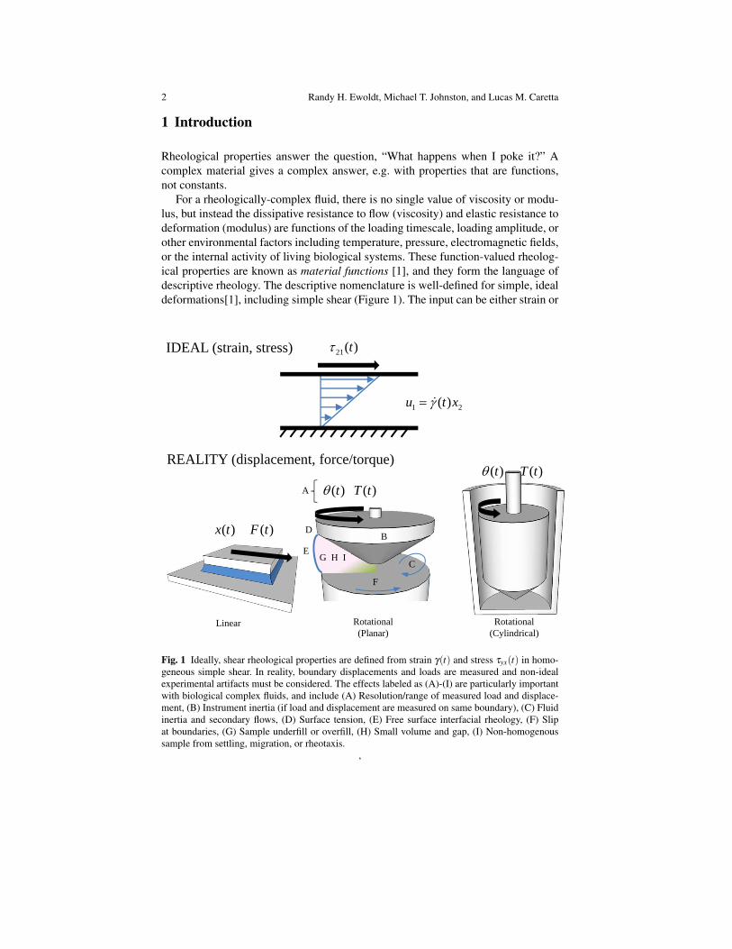
For a rheologically-complex fluid, there is no single value of viscosity or modu-lus, but instead the dissipative resistance to flow (viscosity) and elastic resistance todeformation (modulus) are functions of the loading timescale, loading amplitude, orother environmental factors including temperature, pressure, electromagnetic fields,or the internal activity of living biological systems. These function-valued rheolog-ical properties are known as material functions [1], and they form the language ofdescriptive rheology. The descriptive nomenclature is well-defined for simple, idealdeformations[1], including simple shear (Figure 1). The input can be either strain or

C

IDEAL (strain, stress)

REALITY (displacement, force/torque)

Linear Rotational(Planar)

Rotational(Cylindrical)

G H I

F

D

21( )t

1 2( )u t x

( ) ( )x t F t

( ) ( )t T t

E

A

B

( ) ( )t T t

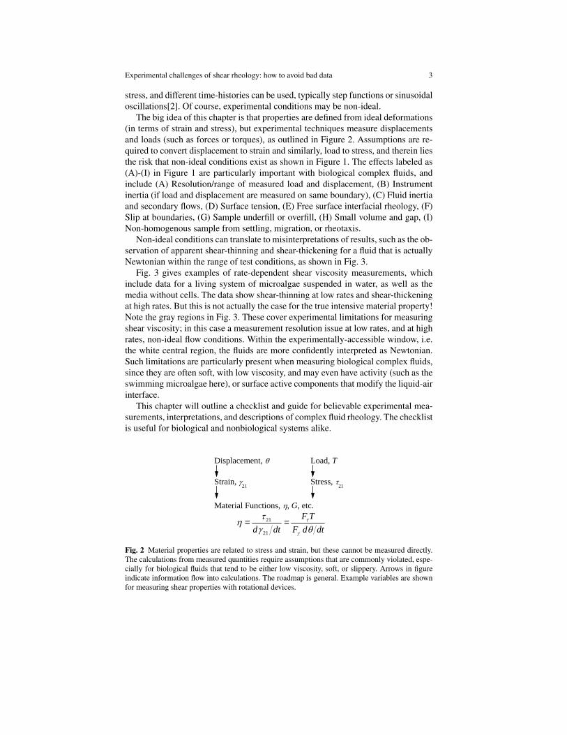
Fig. 1 Ideally, shear rheological properties are defined from strain γ(t) and stress τyx(t) in homo-geneous simple shear. In reality, boundary displacements and loads are measured and non-idealexperimental artifacts must be considered. The effects labeled as (A)-(I) are particularly importantwith biological complex fluids, and include (A) Resolution/range of measured load and displace-ment, (B) Instrument inertia (if load and displacement are measured on same boundary), (C) Fluidinertia and secondary flows, (D) Surface tension, (E) Free surface interfacial rheology, (F) Slipat boundaries, (G) Sample underfill or overfill, (H) Small volume and gap, (I) Non-homogenoussample from settling, migration, or rheotaxis.

,

Experimental challenges of shear rheology: how to avoid bad data 3

stress, and different time-histories can be used, typically step functions or sinusoidaloscillations[2]. Of course, experimental conditions may be non-ideal.

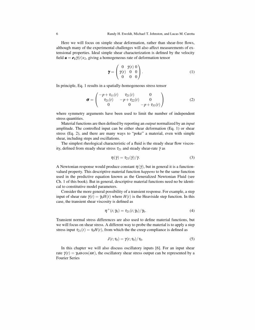
The big idea of this chapter is that properties are defined from ideal deformations(in terms of strain and stress), but experimental techniques measure displacementsand loads (such as forces or torques), as outlined in Figure 2. Assumptions are re-quired to convert displacement to strain and similarly, load to stress, and therein liesthe risk that non-ideal conditions exist as shown in Figure 1. The effects labeled as(A)-(I) in Figure 1 are particularly important with biological complex fluids, andinclude (A) Resolution/range of measured load and displacement, (B) Instrumentinertia (if load and displacement are measured on same boundary), (C) Fluid inertiaand secondary flows, (D) Surface tension, (E) Free surface interfacial rheology, (F)Slip at boundaries, (G) Sample underfill or overfill, (H) Small volume and gap, (I)Non-homogenous sample from settling, migration, or rheotaxis.

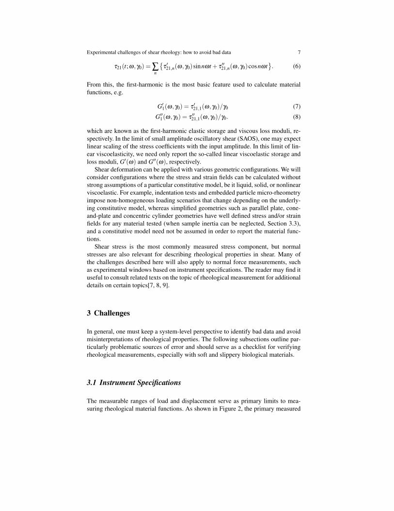
Non-ideal conditions can translate to misinterpretations of results, such as the ob-servation of apparent shear-thinning and shear-thickening for a fluid that is actuallyNewtonian within the range of test conditions, as shown in Fig. 3.

Fig. 3 gives examples of rate-dependent shear viscosity measurements, whichinclude data for a living system of microalgae suspended in water, as well as themedia without cells. The data show shear-thinning at low rates and shear-thickeningat high rates. But this is not actually the case for the true intensive material property!Note the gray regions in Fig. 3. These cover experimental limitations for measuringshear viscosity; in this case a measurement resolution issue at low rates, and at highrates, non-ideal flow conditions. Within the experimentally-accessible window, i.e.the white central region, the fluids are more confidently interpreted as Newtonian.Such limitations are particularly present when measuring biological complex fluids,since they are often soft, with low viscosity, and may even have activity (such as theswimming microalgae here), or surface active components that modify the liquid-airinterface.

This chapter will outline a checklist and guide for believable experimental mea-surements, interpretations, and descriptions of complex fluid rheology. The checklistis useful for biological and nonbiological systems alike.

D i s p l a c e m e n t , L o a d , TS t r a i n , 2 1 S t r e s s , 2 1

M a t e r i a l F u n c t i o n s , , G , e t c .2 1

2 1

F Td d t F d d t

= =

Fig. 2 Material properties are related to stress and strain, but these cannot be measured directly.The calculations from measured quantities require assumptions that are commonly violated, espe-cially for biological fluids that tend to be either low viscosity, soft, or slippery. Arrows in figureindicate information flow into calculations. The roadmap is general. Example variables are shownfor measuring shear properties with rotational devices.


1 1 0 1 0 0 1 0 0 00

1

2

3

Appar

ent Vi

scosity

, a [m

Pa.s]

S h e a r R a t e , [ s - 1 ]

m o t i l e n o n - m o t i l e f r e s h m e d i a R e 2 d e v i a t i o n

l o w - t o r q u el i m i t e f f e c t s

s e c o n d a r y f l o we f f e c t s

Fig. 3 Steady shear flow measurements could be misinterpreted as shear-thinning and shear-thickening if an experimental window is not identified. Here, shown with dilute suspensions ofmotile and non-motile swimming microalgae Dunaliella primolecta compared to fresh media(no cells present). The low-torque limit, described in Section 3.1, is drawn from Eq. 13 usingTmin = 0.1 µN.m. The secondary flow limit, described in Section 3.3, is drawn from Eq. 31 usingRemax = 4. The Re2 line is from the expected increase in torque due to secondary flow, Eq. 29.(Previously unpublished work of authors RHE and LMC.)

For proper context, two important ideas must be kept in mind. First, rheologicalmaterial functions are universally applicable to any class of material. They are usedto describe polymer liquids, polymer solids, colloidal systems, and any other simpleor complex structured fluid of the past, present, or future, so long as the continuumhypothesis is satisfied for the lengthscale of interest. Like other material proper-ties, definitions are independent of the underlying structure (polymeric, colloidal,etc.), yet, the underlying structure can be related to the measured properties throughstructure-property relations specific to material classes[3]. Second, we note that thedescriptive material functions resulting from measurements are not necessarily pre-dictive for more complex deformations, although there are certain limiting caseswhere there is correspondence between descriptive material functions and predic-tive tensorial constitutive equation parameters[4]. Material functions are of courseused to fit existing models (see Ch. 1 of this book), or used to motivate new consti-tutive models.

Here we focus on measurements and the corresponding descriptive quantities. Ofcourse, such measurements are often used for either structure-property relations ormodel selection/fitting of predictive constitutive models. For those follow-up stepsto be successful, the measurements must first be free from errors.

Avoiding bad data is a serious challenge with complex fluids in general and softbiological fluids in particular. Throughout this chapter, three key materials will serve


Fig. 4 Hagfish defense gel (a.k.a. slime) is one extreme case study used here to outline exper-imental rheology challenges. Hagfish produce heroic amounts of slime as a predatory defensemechanism, using a very small amount of exudate ( 0.01 wt% of final gel mass); (a) top-downview of three Atlantic hagfish (Myxine glutinosa) in a large glass beaker; (b) for experiments, exu-date can be collected from an anesthetized hagfish with a pipette and then mixed with seawater toform “hagfish slime,” an ultra-dilute network of polymeric mucus and fibrous protein-based inter-mediate filament threads, shown in (c) with a rotational rheometer geometry in the raised positionafter testing (diameter 28mm). The ultra-soft material pushes experimental limits of low-torque,instrument inertia, and sample inertia, and demonstrates interio-elastic ringing. (Figure adaptedfrom [5])

as examples of soft, watery, or active fluids. This includes (i) actively swimmingmicroalgae in a suspension of aqueous media (Figure 3) (see also Ch. 9 of thisbook on active suspensions), (ii) a biopolymer hagfish defense gel (Figure 4), whichinvolves mucin-like molecules (see Ch. 2 of this book for a discussion of mucins),and (iii) water itself, which is the basis of biological fluids. Material details areoutlined in the Appendix.

2 Background: Material Functions

The theoretical definitions of material functions are based on stress, strain, andstrain-rate components in simple deformation fields. (See Ch. 1 of this book foradditional background on stress and strain-rate tensors). With real measurements,one typically measures loads and displacements at the boundaries of a sample (Fig-ure 1), and the calculation of true stress and strain may be encumbered by the issueslabeled A-I in Figure 1. This chapter summarizes key experimental challenges forcomplex fluids, especially for biological fluids. These experimental challenges mayinvalidate results and sometimes cause measured properties to incorrectly appearnonlinear or non-Newtonian. A useful approach is to identify the experimental win-dows for proper measurements (Figures 3, 6, 5, 10, 11, 14, and 15). The boundariesof these figures will be described in Section 3.


Here we will focus on simple shear deformation, rather than shear-free flows,although many of the experimental challenges will also affect measurements of ex-tensional properties. Ideal simple shear characterization is defined by the velocityfield uuu = eee111γ(t)x2, giving a homogeneous rate of deformation tensor

γγγ =

0 γ(t) 0γ(t) 0 0

0 0 0

. (1)

In principle, Eq. 1 results in a spatially-homogeneous stress tensor

σσσ =

−p+ τ11(t) τ21(t) 0τ21(t) −p+ τ22(t) 0

0 0 −p+ τ33(t)

(2)

where symmetry arguments have been used to limit the number of independentstress quantities.

Material functions are then defined by reporting an output normalized by an inputamplitude. The controlled input can be either shear deformation (Eq. 1) or shearstress (Eq. 2), and there are many ways to “poke” a material, even with simpleshear, including steps and oscillations.

The simplest rheological characteristic of a fluid is the steady shear flow viscos-ity, defined from steady shear stress τ21 and steady shear-rate γ as

η(γ) = τ21(γ)/γ. (3)

A Newtonian response would produce constant η(γ), but in general it is a function-valued property. This descriptive material function happens to be the same functionused in the predictive equation known as the Generalized Newtonian Fluid (seeCh. 1 of this book). But in general, descriptive material functions need no be identi-cal to constitutive model parameters.

Consider the more general possibility of a transient response. For example, a stepinput of shear rate γ(t) = γ0H(t) where H(t) is the Heaviside step function. In thiscase, the transient shear viscosity is defined as

η+(t; γ0) = τ21(t; γ0)/γ0. (4)

Transient normal stress differences are also used to define material functions, butwe will focus on shear stress. A different way to probe the material is to apply a stepstress input τ21(t) = τ0H(t), from which the the creep compliance is defined as

J(t;τ0) = γ(t;τ0)/τ0. (5)

In this chapter we will also discuss oscillatory inputs [6]. For an input shearrate γ(t) = γ0ω cos(ωt), the oscillatory shear stress output can be represented by aFourier Series


τ21(t;ω,γ0) = ∑n

τ′21,n(ω,γ0)sinnωt + τ

′′21,n(ω,γ0)cosnωt

. (6)

From this, the first-harmonic is the most basic feature used to calculate materialfunctions, e.g.

G′1(ω,γ0) = τ′21,1(ω,γ0)/γ0 (7)

G′′1(ω,γ0) = τ′′21,1(ω,γ0)/γ0. (8)

which are known as the first-harmonic elastic storage and viscous loss moduli, re-spectively. In the limit of small amplitude oscillatory shear (SAOS), one may expectlinear scaling of the stress coefficients with the input amplitude. In this limit of lin-ear viscoelasticity, we need only report the so-called linear viscoelastic storage andloss moduli, G′(ω) and G′′(ω), respectively.

Shear deformation can be applied with various geometric configurations. We willconsider configurations where the stress and strain fields can be calculated withoutstrong assumptions of a particular constitutive model, be it liquid, solid, or nonlinearviscoelastic. For example, indentation tests and embedded particle micro-rheometryimpose non-homogeneous loading scenarios that change depending on the underly-ing constitutive model, whereas simplified geometries such as parallel plate, cone-and-plate and concentric cylinder geometries have well defined stress and/or strainfields for any material tested (when sample inertia can be neglected, Section 3.3),and a constitutive model need not be assumed in order to report the material func-tions.

Shear stress is the most commonly measured stress component, but normalstresses are also relevant for describing rheological properties in shear. Many ofthe challenges described here will also apply to normal force measurements, suchas experimental windows based on instrument specifications. The reader may find ituseful to consult related texts on the topic of rheological measurement for additionaldetails on certain topics[7, 8, 9].

3 Challenges

In general, one must keep a system-level perspective to identify bad data and avoidmisinterpretations of rheological properties. The following subsections outline par-ticularly problematic sources of error and should serve as a checklist for verifyingrheological measurements, especially with soft and slippery biological materials.

3.1 Instrument Specifications

The measurable ranges of load and displacement serve as primary limits to mea-suring rheological material functions. As shown in Figure 2, the primary measured


variables for rotational rheometry include torque T , displacement θ , and rotationalvelocity Ω . We will use the following notation for conversion factors to calculatestress and deformation

τ21 = Fτ T (9)γ = Fγ θ (10)

γ = Fγ θ = Fγ Ω . (11)

The minimum torque is typically the most important limitation for soft biologicalsystems. Minimum torque is often specified by instrument manufacturers, but canoften be higher due to other effects (such as surface tension producing torque, Sec-tion 3.4).

To identify experimental limitations, we will use the approach of drawing bound-ary lines within the coordinate axes used to report material functions, as done inFigure 3. First, write the reported material functions in terms of the measured quan-tities and conversion factors. For example, steady shear viscosity from Eq. 3 wouldbe

η(γ) =τ21(γ)

γ=

Fτ

Fγ

T (Ω)

Ω. (12)

Next, we state the condition for acceptable data that measured torque is above someminimum limit, T > Tmin. Substituting Eq. 12 into the condition T > Tmin providesthe criteria

η >Fτ Tmin

γ. (13)

for avoiding bad data. This equation was used in Figure 3 for the cone plate geome-try Fτ = 3/(2πR3) where R is the cone radius and Tmin = 0.1 µN.m was used.

The appropriate value for Tmin can sometimes be larger than instrument speci-fication, e.g. with dilute polymers in aqueous solution[10, 11, 12]. Recent resultsshow that surface tension torque may be responsible for torque limits higher thaninstrument specifications[13], as discussed in Section 3.4. The limit of minimummeasurable viscosity decreases as the shear rate is increased. This is because thelimit corresponds to a minimum measurable shear stress τ21,min = Fτ Tmin, and vis-cosity is calculated as shear stress divided by shear rate.

A similar downward sloping low-torque limit appears for other material func-tions that are plotted as a function of an amplitude. Consider viscoelastic modulias a function of strain amplitude (Figure 5), for which the low-torque limit sets theminimum measurable viscoelastic moduli

Gmin =Fτ Tmin

γ0. (14)

where Gmin refers to either G′ or G′′. For the concentric cylinder geometry (sin-gle gap) used in Figs. 5–6, Fτ = 1/(2πR2L) with minimum torque in oscillationTmin = 0.003µN.m as specified by the manufacturer (TA Instruments, AR-G2). In


1 0 - 4 1 0 - 3 1 0 - 2 1 0 - 1 1 0 0 1 0 1 1 0 21 0 - 4

1 0 - 3

1 0 - 2

1 0 - 1

1 0 0

G "

A m p l i t u d e s w e e p a t = 0 . 1 5 r a d / s

Viscoe

lastic

Modul

i [Pa]

S t r a i n A m p l i t u d e 0 [ - ]

l o w - t o r q u e l i m i t e f f e c t s

G '

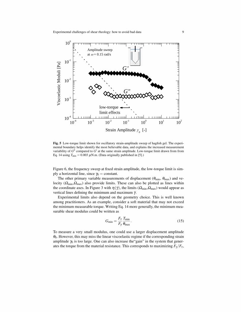
Fig. 5 Low-torque limit shown for oscillatory strain-amplitude sweep of hagfish gel. The experi-mental boundary helps identify the most believable data, and explains the increased measurementvariability of G′′ compared to G′ at the same strain amplitude. Low-torque limit drawn from fromEq. 14 using Tmin = 0.003 µN.m. (Data originally published in [5].)

Figure 6, the frequency sweep at fixed strain amplitude, the low-torque limit is sim-ply a horizontal line, since γ0 = constant.

The other primary variable measurements of displacement (θmin, θmax) and ve-locity (Ωmin,Ωmax) also provide limits. These can also be plotted as lines withinthe coordinate axes. In Figure 3 with η(γ), the limits (Ωmin,Ωmax) would appear asvertical lines defining the minimum and maximum γ .

Experimental limits also depend on the geometry choice. This is well knownamong practitioners. As an example, consider a soft material that may not exceedthe minimum measurable torque. Writing Eq. 14 more generally, the minimum mea-surable shear modulus could be written as

Gmin =Fτ

Fγ

Tmin

θmax. (15)

To measure a very small modulus, one could use a larger displacement amplitudeθ0. However, this may miss the linear viscoelastic regime if the corresponding strainamplitude γ0 is too large. One can also increase the“gain” in the system that gener-ates the torque from the material resistance. This corresponds to maximizing Fγ/Fτ ,


1 0 - 2 1 0 - 1 1 0 0 1 0 1 1 0 21 0 - 4

1 0 - 3

1 0 - 2

1 0 - 1

1 0 0

Viscoe

lastic

Modul

i [Pa]

s a m p l e i n e r t i a e f f e c t s

2i n e r t i at o r q u e

r e s p o n s e

F r e q u e n c y s w e e pa t 0 = 0 . 1 0

F r e q u e n c y , [ r a d / s ]

i n s t r u m e n ti n e r t i a e f f e c t s

l o w - t o r q u e l i m i t

G "

G '

Fig. 6 Low-torque and instrument-inertia limits shown for oscillatory frequency sweep of hagfishgel. Low-torque limit from Eq. 14 with constant γ0; instrument-inertia limit from Eq. 18; sampleinertia limit from Eq. 26. The inertial torque response (solid line) is from Eq. 20 with ε = 0.01being the error in the instrument inertia torque correction. Gray circles indicate when raw phaseangle jumps from < 15 to > 130 which is also an indication that instrument inertia correctionsmust be made. (Data originally published in [5].)

e.g. for a cone-plate system Fγ/Fτ = 2πR3/(3β ), where β is the small cone angle.For a soft material, one may choose a large R to generate sufficient torque to makethe measurement, or switch to a different geometry with a larger value of Fγ/Fτ ,such as concentric cylinders used in Figs. 5–7 for the soft hagfish defense gel.

Geometry choices influence other challenges, and there may be trade-offs be-tween different experimental limitations. One issue is inertia of the moving instru-ment components, if the torque is being measured at the moving boundary. This isoutlined in the following section.

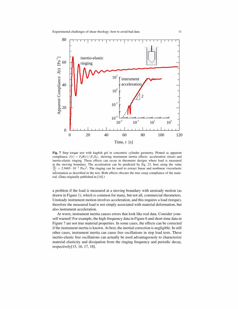
3.2 Instrument Inertia

Instrument inertia causes experimental artifacts under transient conditions. This in-cludes oscillatory tests (e.g. limiting the high-frequency data in Figure 6) and steptests (e.g. influencing the short time creep compliance data in Figure 7). This is only


0 2 0 4 0 6 0 8 0 1 0 0 1 2 00

2 0

4 0

6 0

8 0

1 0 - 3 1 0 - 1 1 0 1 1 0 31 0 - 4

1 0 - 2

1 0 0

1 0 2

2

i n s t r u m e n ta c c e l e r a t i o n

i n e r t i o - e l a s t i cr i n g i n g

Appar

ent Co

mplia

nce J(

t) [Pa

-1 ]

T i m e , t [ s ]Fig. 7 Step torque test with hagfish gel in concentric cylinder geometry. Plotted as apparentcompliance J(t) = Fγ θ(t)/(Fτ T0), showing instrument inertia effects: acceleration (inset) andinertio-elastic ringing. These effects can occur in rheometer designs where load is measuredat the moving boundary. The acceleration can be predicted by Eq. 23, here using the valueIFτ

Fγ= 2.9465 · 10−2 Pa.s2. The ringing can be used to extract linear and nonlinear viscoelastic

information as described in the text. Both effects obscure the true creep compliance of the mate-rial. (Data originally published in [14].)

a problem if the load is measured at a moving boundary with unsteady motion (asdrawn in Figure 1), which is common for many, but not all, commercial rheometers.Unsteady instrument motion involves acceleration, and this requires a load (torque),therefore the measured load is not simply associated with material deformation, butalso instrument acceleration.

At worst, instrument inertia causes errors that look like real data. Consider your-self warned! For example, the high-frequency data in Figure 6 and short-time data inFigure 7 are not true material properties. In some cases, the effects can be correctedif the instrument inertia is known. At best, the inertial correction is negligible. In stillother cases, instrument inertia can cause free oscillations in step load tests. Theseinertio-elastic free oscillations can actually be used advantageously to characterizematerial elasticity and dissipation from the ringing frequency and periodic decay,respectively[15, 16, 17, 18].


Biomaterials can be exceedingly soft, and instrument inertia artifacts are ex-aggerated for very soft materials As examples of softness, the elastic modulus ofhagfish gel is G′ ≈ 0.2 Pa (Figure 6-7), microtubule networks have a plateau mod-ulus, G′ ∼ 0.4− 20 Pa [19], vitreous gel G′ ≈ 2 Pa [20], actin networks as lowas G′ ≈ 1 Pa [21, 22], fibrin at low concentration G′ ≈ 10 Pa [23], and collagen-hyaluronic acid interpenetrating polymer network hydrogels G′ ≈ 1− 100 Pa [24].In any soft material, instrument inertia must be carefully considered with transientrheological measurements.

To avoid bad data in oscillatory shear, the “material torque” should exceed the“instrument-inertia torque”. Thus, the criteria for good data is satisfied under thefollowing condition

Tmaterial > Tinertia (16)Gγ0

Fτ

> Iθ0ω2 (17)

G >IFτ

Fγ

ω2 (18)

where the variable G represents either G′ or G′′ in oscillation. Eq. 18 is used todraw the “instrument inertia” boundary in Figure 6 for the onset of instrument-inertia effects. For the experiment in Figure 6, with a concentric cylinder geometry,IFτ

Fγ= 2.9465 ·10−2 Pa.s2. Eq. 18 corresponds to the jump in raw phase. Instrument

inertia corrections can be made beyond this point, and this requires the subtractionof the instrument inertia torque from the single. This is reasonable to a point, butartifacts may eventually appear, e.g. with moduli increasing close to G′ ∼G′′ ∼ ω2.This signature can be explained by inertia effects.

Some of the most prevalent undiagnosed errors in rheometry involve artifacts inhigh frequency oscillatory measurements. One should be very careful when inter-preting high-frequency data. For example, without drawing the instrument-inertiaboundary line in Figure 6, one might be tempted to interpret a curious power lawscaling of viscoelastic properties as a function of frequency. However, this data athigh-frequency is completely associated with instrument inertia, and not at all amaterial property.

An instrument-inertia artifact at high frequency is most easily diagnosed by look-ing at the raw phase difference between the oscillating displacement and torque sig-nals, and being critical of data points with raw phase > 90. To see why, considerthat a purely elastic material response would have load proportional to displacement,T ∼ θ , a purely viscous material gives T ∼ θ , and a purely inertial effect T ∼ θ .For time periodic oscillatory signals T (t) and θ(t), this corresponds to phase dif-ferences of 0, 90, and 180, respectively. Without instrument inertia effects, thephase would be limited to the viscoelastic range 0 < δ < 90. So, when this rawphase is > 90, instrument inertia must be playing a role. Corrections can be madeby calibrating the rotational inertia, and subtracting the expected inertial torque fromthe total signal (as done for the data in Figure 6). But, this become exceedingly diffi-

RHE

Highlight

should be "0.02 Pa"


cult at large values of raw phase when the inertial torque dominates the total torquesignal.

Inertia corrections are not 100% perfect, and this explains the specific signatureat high frequency of G′ ∼ G′′ ∼ ω2. One expects inertial torque T = Iθ , and forθ(t) = θ0 sin(ωt) this is

T0 = Iθ0ω2. (19)

This can be subtracted from the measured signal, but if the subtraction is not exact,then some of this inertial torque will remain in the processed signal, say εT0 where ε

is (hopefully) a small number. Translated to material properties, this would produceapparent viscoelastic moduli

G =Fτ(εT0)

Fγ θ0= ε

Fτ IFγ

ω2. (20)

With ε = 0.01, Eq. 20 explains the high-frequency signature in Figure 6. Therefore,even with inertia corrections, viscoelastic moduli will eventually have frequency-dependent power-law scaling that approaches G′ ∼ G′′ ∼ ω2, since they are calcu-lated from a torque signal that is increasingly dominated by inertia and correctionsare only precise to within factor of ε .

Instrument inertia affects high frequency oscillation data, as well as short timedata in step tests. For creep tests (step load input), the instrument inertia can signif-icantly alter the displacement response (Figure 7, hagfish gel). This includes (i) thetime required to accelerate and (ii) free oscillations via “inertio-elastic” ringing, inwhich the sample elasticity couples with the finite instrument inertia to “ring” at aresonant frequency, just like a mass at the end of a spring[15, 17, 18, 25]. A care-ful analysis of the inertio-elastic oscillations can reveal both linear and nonlinearviscoelastic properties of the sample[5, 18].

By conservation of momentum, the measured dynamic load must satisfy

T (t) = Iθ(t)+ τ21(t)/Fτ (21)

where we have considered a rotational rheometer with instrument inertia I. For astep torque T (t) = T0H(t), the initial conditions at t = 0 are θ = 0, θ = 0, andtypically τ21 = 0 if starting from rest. Initially, the applied torque is dominated bythe acceleration term in Eq. 21, since the sample stress term is initially zero andonly appears as strain and strain rate increase above zero. The creep response thenalways has the following form in the limit of short time[17],

θ(t) =12

T0

It2 + ... (22)

Converting this to the apparent material function J(t)

J(t) =γ(t)τ0

=12

Fγ

Fτ It2 + ... (23)


which shows the general short time instrument acceleration artifact, independent ofapplied torque when plotted as apparent compliance J(t). This is shown in the insetof Figure 7 for the soft hagfish gel.

Inertio-elastic ringing analysis can probe both linear viscoelasticity [15, 17] andnonlinear viscoelasticity [5, 18] in novel ways. Such analysis requires the assump-tion of an underlying constitutive model for τ21(t) in Eq. 21, e.g. a three-elementfluid (Jeffreys), or two-element solid (Kelvin-Voigt). Detailed calculations associ-ated with the inertio-elastic ringing analysis can be found in the references above.

To avoid the instrument inertia effects discussed in this section, one can measurethe load (torque) at the stationary boundary, e.g. with a force rebalancing transducer,rather than measuring load at the moving boundary, e.g. through a motor. This re-quires more complex instrumentation to separate the imposed displacement from themeasured load, but such separated- motor-transducer instruments are commerciallyavailable. These setups can eliminate important errors due to instrument inertia in-cluding the accurate measurement of stress jumps in response to step displacementinputs[26].

3.3 Fluid Inertia and Secondary Flows

Even if instrument inertia is eliminated, the sample itself will always have finiteinertia which can produce artifacts from momentum diffusion, viscoelastic waves,and secondary flows, all of which can violate the assumption of homogeneous sim-ple shear deformation in Eq. 1. Purely elastic instability can also produce secondaryflows even in the limit of vanishing Reynolds number [27, 28, 29, 30]. This sectionwill discuss the symptoms of both wave propagation and secondary flows, and howto identify experimental limits due to these artifacts.

3.3.1 Wave propagation at high frequencies and short timescales

The assumption of homogeneous simple shear strain is violated when there arewaves propagating through the material. Propagating waves may come from eitherviscous momentum diffusion or elastic shear waves, or both for viscoelastic materi-als in general.

The general criteria for suitably homogeneous strain in the velocity gradient di-rection is that the wavelength l of any propagating wave should be much larger thanthe geometry gap D

l D (24)

so that, in the gap region, the velocity field is unaffected by the propagatingwave [31]. Two key questions must be answered: (i) how much smaller must thegap D be for tolerable errors, and (ii) how can the wavelength l be calculated. Thewavelength l depends on material properties and the frequency (timescale) of mo-


tion. Most importantly, l decreases with high driving frequency, and we thereforeexpect wave propagation issues at high frequency and short timescales.

Schrag gave a detailed analysis of linear viscoelastic wave propagation [31],showing that linear viscoelastic shear waves between a moving boundary and a fixedreflecting boundary have wavelength

l =1

cos(δ/2)

(|G∗|

ρ

)1/2 2π

ω(25)

where ω is the driving frequency, |G∗|=√

G′2 +G′′2 is the magnitude of the com-plex modulus, δ is the viscoelastic phase angle, and ρ is the fluid density. The scal-ing in Eq. 25 is l ∼ cT where c is the wavespeed c∼ (|G∗|/ρ)1/2 and T = 2π/ω

is the wave period. Using the criteria l ≥ 10D to avoid errors of possibly 10% [31],along with Eq. 25, we can identify an approximate edge of the experimental windowfor plots of viscoelastic moduli,

|G∗|>(

102π

)2

cos2(δ/2)ρω2D2. (26)

which is used in Fig. 6 to identify the “sample inertia limit,” using a value cos2( δ

2 ) =

1. Equation 26 scales as |G∗| ∼ ρω2D2, showing the important sensitivity to bothdriving frequency ω and geometry gap D. Higher frequencies are problematic.Smaller gas are helpful. The numerical front factor has weak dependence on δ , since12 < cos2( δ

2 ) < 1. The more sensitive number is the factor by which l > D. Moreprecise experiments require a larger separation of these lengthscales, as detailed inSchrag [31] (his Table 1). Whatever the front factor, the shape of the experimentallimit will still be the same, scaling as |G∗| ∼ ρω2D2. The sample inertia impactsmeasurement at high frequency and low modulus, and therefore soft gels and lowviscosity fluids will have greater propensity for sample inertia effects.

Although strain amplitude does not appear explicitly in Eq. 26, fluid inertia prob-lems can appear due to large amplitude oscillations [32], even with constant forcingfrequency. For these nonlinear tests, one can conceptually think about |G∗| chang-ing in the nonlinear regime, which would influence the wave propagation speed andtherefore the wavelength l. When large amplitude oscillatory shear strain softens asample (decreasing |G∗| which is typical for polymer melts), then the sample inertiaissue will become more problematic at large strain amplitudes. This is consistentwith detailed studies in the literature on flexible polymers [32]. However, if a sam-ple becomes more stiff in the nonlinear regime (increasing |G∗| which is typicalof semi-flexible biopolymer gels [33]), then one could argue that the inertia arti-fact may actually be less problematic due to increasing viscoelastic wavelength l.This possibility, however, has not yet been studied in any detail. One challenge foruniversal analysis of nonlinear viscoelastic measurements with wave propagation isthat no universal constitutive equation exists for nonlinear viscoelasticity.

The experimental boundary line defined by Eq. 26 should serve as a generalguideline to identify possible experimental windows due to shear waves when mea-


suring oscillatory shear material functions. It is useful in linear viscoelastic plots,e.g. G′(ω),G′′(ω) (as in Fig. 6), and may also be useful to estimate the boundaryfor nonlinear tests, e.g. large-amplitude oscillatory shear (LAOS) tests in terms of|G∗1|(γ0). For all these cases, the artifact of viscoelastic waves will limit measure-ment of low modulus and high frequency data.

3.3.2 Secondary flows at high velocity

Sample inertia can also cause non-ideal velocity fields during steady flow. Even be-fore turbulent flow, high velocities can cause secondary flows superposed on theprimary simple shear flow due to finite sample inertia and curved streamlines inunstable configurations. This includes cylindrical geometries with a rotating innercylinder and planar geometries including cone-plate and parallel disk flow. In eachcase, secondary flow increases the measured torque and therefore incorrectly in-creases the apparent viscosity of the fluid. For example, a Newtonian fluid withsecondary flow present would incorrectly appear as shear-thickening, since the sec-ondary flow effects grow with increasing velocity. This is observed in Fig. 3 withthe microalgae suspension at high shear rates.

Concentric cylinder measurements have a well-known secondary flow instabilitythat appears when the inner cylinder is rotating at sufficiently large velocity Ω .Known as Taylor-Couette flow after the initial work of G.I. Taylor [34], the inertialinstability causes axisymmetric vortices. The stability criteria is well established forNewtonian fluids in the limit of small gaps. It is based on a sufficiently small Taylornumber Ta [35, 36]

Ta =ρ2Ω 2(Ro−Ri)

3Ri

η2 < 1700 (27)

where Ri is the inner radius moving at angular velocity Ω , and Ro is the fixed outerradius. The criteria has been mapped for co-rotating and counter-rotating cylindersas well, but the most useful criteria for shear rheometry is given in Eq. 27. Thereis some evidence that non-Newtonian polymer solutions increase the critical Tay-lor number, so that Eq. 27 is a conservative estimate for experimental rheologi-cal measurements [8]. To draw an experimental boundary line on a plot of viscos-ity versus shear rate η(γ), re-arrange Eq. 27 and use the definition of shear rateγ = ΩRi/(Ro−Ri). This gives the condition

η >(Ro−Ri)

5/2

1700R1/2i

ργ. (28)

to avoid Taylor vortices. The criteria emphasizes that low viscosity fluids are moreprone to this secondary flow and that small gaps are very helpful in the geometrydesign. The scaling η ∼ γ defines the shape of the boundary on a plot of η(γ) andlimits high shear rate measurements. As a quantitative example of an experimentallimit for the concentric cylinder geometry, consider properties typical of biolog-ical fluids, density ρ = 103 kg/m3 and viscosity near water η = 1 mPa.s. For a

RHE

Highlight

entire denominator should be raised to 1/2 power: (1700*R_i)^1/2


nominal concentric cylinder geometry with gap (Ro−Ri) = 1 mm and inner radiusRi = 11.8 mm (based on the ISO 3219 standard with Ro/Ri = 1.0847 [37]), Eq. 28can be re-arranged to show the shear rate is limited to γ < 5.8 ·103 s−1. This is rea-sonably high, but of course will change depending on the actual viscosity and sizeof geometry being used.

Cone-plate and parallel disk geometries have a secondary flow that is alwayspresent at finite rotational velocity [38] (the critical Taylor number does not applyto these geometries). Here, centrifugal effects create a radial velocity componentwith outward flow at the rotating boundary. Due to conservation of mass this causesinward flow at the stationary boundary. (Highly elastic liquids can change this sce-nario as discussed in the following section.) For the Newtonian case, the strengthof the flow is based on a Reynolds number. The secondary flow increases the mea-sured torque, and this can be used to set a criteria and draw experimental limits formeasurement. For Newtonian fluids with cone-plate or parallel disk geometry, themeasured torque T is predicted to depend on the Reynolds number as [39]

TT0

= 1+3

4900Re2 (29)

where T0 is ideal torque due to shear flow alone, and Re is Reynolds number definedas

Re =ρΩL2

η0(30)

where L is the representative gap lengthscale. For cone-plate, L = βR where β isthe angle between the cone and plate, and for a parallel plate, L = H where His the gap. For a given error bound on T/T0, we can identify a critical Reynoldsnumber Recrit. For example with 1% error, i.e. T/T0 = 1.01, the critical Reynoldsnumber is Recrit = 4. This clearly occurs before turbulence could be sustained [38],and therefore sets the experimental boundary for rheological measurements. Usingthe criteria Re < Recrit, and the definition of shear rate γ = ΩR/L, results in anexperimental limit that can be shown on plots of steady shear viscosity η(γ),

η >L3/RRecrit

ργ (31)

which is used in Figure 3 to draw the “secondary flow limit” line, using Recrit = 4and L = βR for the cone-plate geometry. Figure 3 also shows the expected apparentshear-thickening of the shear viscosity, based on Eq. 29 and converting to apparentviscosity. Eq. 31 shows the scaling η ∼ ργ , similar to the shape of the boundarywith concentric cylinders and the Taylor-Couette instability, Eq. 28.

In all the rotational geometries discussed here, lower viscosity fluids have asmaller experimental window with limitations at high shear rate due to secondaryflow.


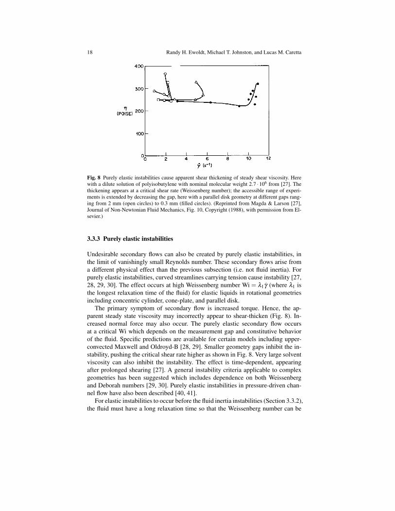
Fig. 8 Purely elastic instabilities cause apparent shear thickening of steady shear viscosity. Herewith a dilute solution of polyisobutylene with nominal molecular weight 2.7 · 106 from [27]. Thethickening appears at a critical shear rate (Weissenberg number); the accessible range of experi-ments is extended by decreasing the gap, here with a parallel disk geometry at different gaps rang-ing from 2 mm (open circles) to 0.3 mm (filled circles). (Reprinted from Magda & Larson [27],Journal of Non-Newtonian Fluid Mechanics, Fig. 10, Copyright (1988), with permission from El-sevier.)

3.3.3 Purely elastic instabilities

Undesirable secondary flows can also be created by purely elastic instabilities, inthe limit of vanishingly small Reynolds number. These secondary flows arise froma different physical effect than the previous subsection (i.e. not fluid inertia). Forpurely elastic instabilities, curved streamlines carrying tension cause instability [27,28, 29, 30]. The effect occurs at high Weissenberg number Wi = λ1γ (where λ1 isthe longest relaxation time of the fluid) for elastic liquids in rotational geometriesincluding concentric cylinder, cone-plate, and parallel disk.

The primary symptom of secondary flow is increased torque. Hence, the ap-parent steady state viscosity may incorrectly appear to shear-thicken (Fig. 8). In-creased normal force may also occur. The purely elastic secondary flow occursat a critical Wi which depends on the measurement gap and constitutive behaviorof the fluid. Specific predictions are available for certain models including upper-convected Maxwell and Oldroyd-B [28, 29]. Smaller geometry gaps inhibit the in-stability, pushing the critical shear rate higher as shown in Fig. 8. Very large solventviscosity can also inhibit the instability. The effect is time-dependent, appearingafter prolonged shearing [27]. A general instability criteria applicable to complexgeometries has been suggested which includes dependence on both Weissenbergand Deborah numbers [29, 30]. Purely elastic instabilities in pressure-driven chan-nel flow have also been described [40, 41].

For elastic instabilities to occur before the fluid inertia instabilities (Section 3.3.2),the fluid must have a long relaxation time so that the Weissenberg number can be


s i d e v i e w s

b o t t o m v i e w s

R = c o n s t a n tΨ = c o n s t a n t

Ψ(s )Ψ(s )Ψ

R (s )R (s )

I d e a l N o n - i d e a l

F r e e S u r f a c e

R

R = c o n s t a n tΨ = c o n s t a n t

Fig. 9 Contact line and interface angle: ideal versus nonideal. Nonideal asymmetries are exag-gerated compared to typical loading and can also occur as a result of overfilling. The nonidealcondition may create artifacts of apparent shear thinning due to the presence of a constant surfacetension torque. (Figure adapted from [13].)

large while Reynolds number or Taylor number is low. For polymeric systems in-cluding biological fluids, elastic instabilities are relevant with high molecular weightpolymers in solution.

For all secondary flows, due to either fluid inertia (Section 3.3.2) or fluid elas-ticity (this subsection), the symptoms are similar: increased viscosity at high shearrates, as seen in Fig. 3 and Fig. 8. These effects limit the high shear-rate experimentalrange for measuring simple shear rheological properties, and tempt misinterpreta-tion of apparent shear-thickening at high rates.

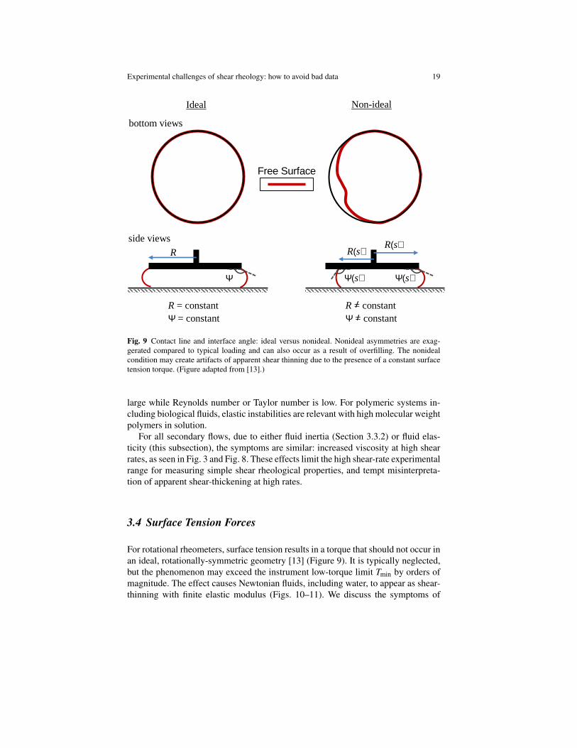
3.4 Surface Tension Forces

For rotational rheometers, surface tension results in a torque that should not occur inan ideal, rotationally-symmetric geometry [13] (Figure 9). It is typically neglected,but the phenomenon may exceed the instrument low-torque limit Tmin by orders ofmagnitude. The effect causes Newtonian fluids, including water, to appear as shear-thinning with finite elastic modulus (Figs. 10–11). We discuss the symptoms of


1 0 - 1 1 0 0 1 0 1 1 0 2 1 0 31 0 - 1

1 0 0

1 0 1

1 0 2

1 0 3

s u r f a c e t e n s i o n l o w - t o r q u e l i m i t ( e x t r e m e c a s e )

i n s t r u m e n t l o w - t o r q u e l i m i t

( b ) S y m p t o m : a p p a r e n t s h e a r - t h i n n i n g v i s c o s i t y

S h e a r R a t e , [ s - 1 ]

Appar

ent Vi

scosity

, a [m

Pa.s]

01

3

1 0 - 3 1 0 - 2 1 0 - 1 1 0 0 1 0 11 0 - 3

1 0 - 2

1 0 - 1

1 0 0

1 0 1

1 0 2

s u r f a c e t e n s i o nl o w - t o r q u e l i m i t ( e x t r e m e c a s e )

3 D r o p l e t s1 D r o p l e t0 D r o p l e t s

( a ) S u r f a c e t e n s i o n t o r q u e p l a t e a u s

3

10To

rque, T

(µN.m

)

V e l o c i t y , Ω ( r a d / s )

v i e w sf r o mb e l o w

i n s t r u m e n tl o w - t o r q u e l i m i t

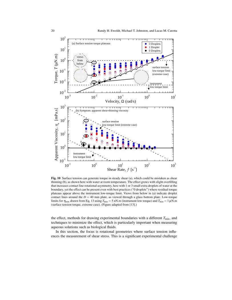
Fig. 10 Surface tension can generate torque in steady shear (a), which could be mistaken as shearthinning (b), as shown here with water at room temperature. The effect grows with slight overfillingthat increases contact line rotational asymmetry, here with 1 or 3 small extra droplets of water at theboundary, yet the effect can be present even with best practices (“0 droplets”) where residual torqueplateaus appear above the instrument low-torque limit. Views from below in (a) indicate dropletcontact lines around the D = 40 mm plate, as viewed through a glass bottom plate. Low-torquelimits for ηmin drawn from Eq. 13 using Tmin = 5 nN.m (instrument low torque) and Tmin = 1 µN.m(surface tension torque, extreme case). (Figure adapted from [13].)

the effect, methods for drawing experimental boundaries with a different Tmin, andtechniques to minimize the effect, which is particularly important when measuringaqueous solutions such as biological fluids.

In this section, the focus is rotational geometries where surface tension influ-ences the measurement of shear stress. This is a significant experimental challenge


1 0 - 2 1 0 - 1 1 0 0 1 0 1 1 0 21 0 - 5

1 0 - 4

1 0 - 3

1 0 - 2

1 0 - 1

( b ) A p p a r e n t t h i n n i n g f r o m s u r f a c e t e n s i o n

Dynam

ic Visc

osity,

' (P

a.s)

F r e q u e n c y , ( r a d / s )

i n s t r u m e n ti n e r t i a l i m i t

i n s t r u m e n tl o w - t o r q u e l i m i t

4 5 9 µL4 9 5 µL

4 9 0 µL

1 0 - 61 0 - 51 0 - 41 0 - 31 0 - 21 0 - 11 0 01 0 1

4 9 0 µL

4 9 5 µL4 5 9 µL

Elastic

Mod

ulus, G

' (Pa

) i n s t r u m e n ti n e r t i a l i m i t

i n s t r u m e n t l o w - t o r q u e l i m i t

( a ) E l a s t i c i t y f r o m s u r f a c e t e n s i o n

v i e w f r o mb e l o w

Fig. 11 Surface tension can generate torque in oscillatory shear, which could be mistaken as shearelasticity (a) and non-constant dynamic modulus (b), as shown here with water at room tempera-ture. Slight underfill or overfill can break contact line rotational symmetry (sample volume 459–495µL for a D = 60 mm steel cone), as shown in the inset view from below at 459µL. Oscillatorystrain amplitude γ0 = 100%. Instrument low torque limit for G′min and η ′min from Eq. 14 withTmin = 0.5 nN.m in oscillation, and instrument inertia limit for for G′min and η ′min from Eq. 18using IFτ

Fγ= 3 ·10−3 Pa.s2. (Figure adapted from [13].)

for measuring soft, active, or low viscosity biological fluids. Related issues not dis-cussed here include (i) normal force from surface tension [42, 43] which is highlydependent on meniscus shape [44, 45, 46]; (ii) sliding plate instruments which di-late free surface area and cause surface tension artifacts in shear stress calcula-tions [47, 48, 49]; and (iii) surface rheology artifacts from films of surface activecomponents [50, 51] which will be discussed in the next section 3.5.


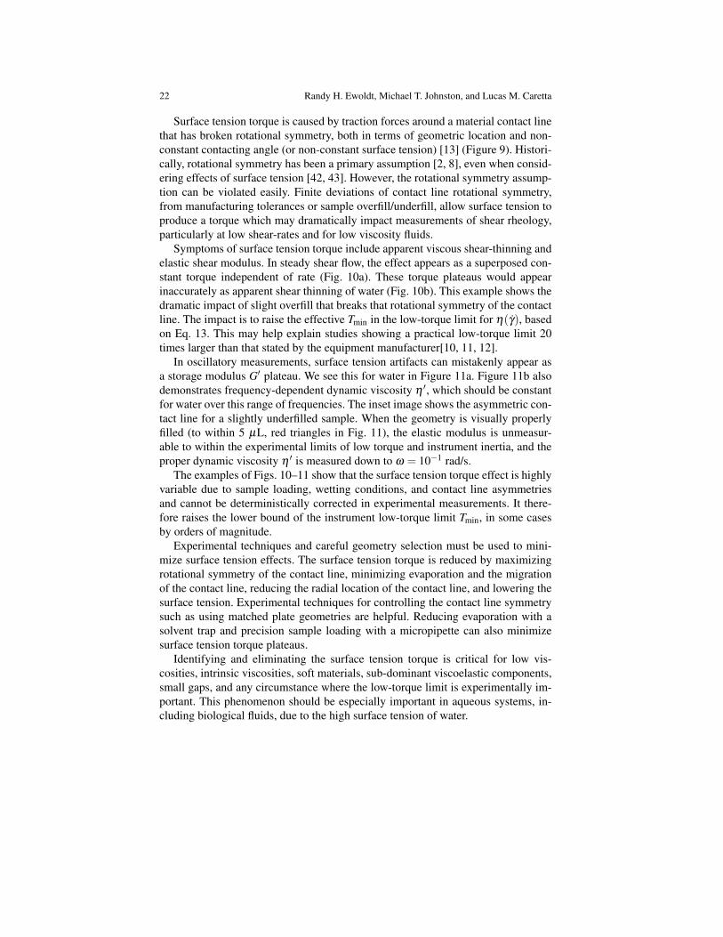
Surface tension torque is caused by traction forces around a material contact linethat has broken rotational symmetry, both in terms of geometric location and non-constant contacting angle (or non-constant surface tension) [13] (Figure 9). Histori-cally, rotational symmetry has been a primary assumption [2, 8], even when consid-ering effects of surface tension [42, 43]. However, the rotational symmetry assump-tion can be violated easily. Finite deviations of contact line rotational symmetry,from manufacturing tolerances or sample overfill/underfill, allow surface tension toproduce a torque which may dramatically impact measurements of shear rheology,particularly at low shear-rates and for low viscosity fluids.

Symptoms of surface tension torque include apparent viscous shear-thinning andelastic shear modulus. In steady shear flow, the effect appears as a superposed con-stant torque independent of rate (Fig. 10a). These torque plateaus would appearinaccurately as apparent shear thinning of water (Fig. 10b). This example shows thedramatic impact of slight overfill that breaks that rotational symmetry of the contactline. The impact is to raise the effective Tmin in the low-torque limit for η(γ), basedon Eq. 13. This may help explain studies showing a practical low-torque limit 20times larger than that stated by the equipment manufacturer[10, 11, 12].

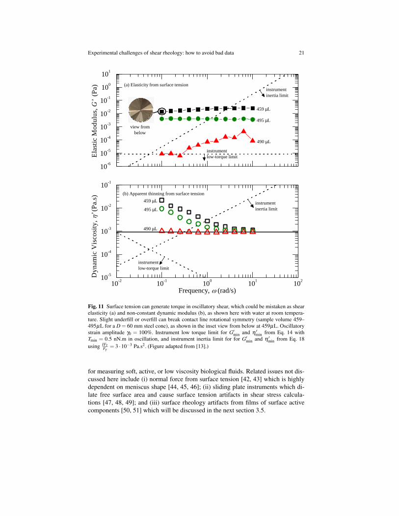
In oscillatory measurements, surface tension artifacts can mistakenly appear asa storage modulus G′ plateau. We see this for water in Figure 11a. Figure 11b alsodemonstrates frequency-dependent dynamic viscosity η ′, which should be constantfor water over this range of frequencies. The inset image shows the asymmetric con-tact line for a slightly underfilled sample. When the geometry is visually properlyfilled (to within 5 µL, red triangles in Fig. 11), the elastic modulus is unmeasur-able to within the experimental limits of low torque and instrument inertia, and theproper dynamic viscosity η ′ is measured down to ω = 10−1 rad/s.

The examples of Figs. 10–11 show that the surface tension torque effect is highlyvariable due to sample loading, wetting conditions, and contact line asymmetriesand cannot be deterministically corrected in experimental measurements. It there-fore raises the lower bound of the instrument low-torque limit Tmin, in some casesby orders of magnitude.

Experimental techniques and careful geometry selection must be used to mini-mize surface tension effects. The surface tension torque is reduced by maximizingrotational symmetry of the contact line, minimizing evaporation and the migrationof the contact line, reducing the radial location of the contact line, and lowering thesurface tension. Experimental techniques for controlling the contact line symmetrysuch as using matched plate geometries are helpful. Reducing evaporation with asolvent trap and precision sample loading with a micropipette can also minimizesurface tension torque plateaus.

Identifying and eliminating the surface tension torque is critical for low vis-cosities, intrinsic viscosities, soft materials, sub-dominant viscoelastic components,small gaps, and any circumstance where the low-torque limit is experimentally im-portant. This phenomenon should be especially important in aqueous systems, in-cluding biological fluids, due to the high surface tension of water.


1 0 0 1 0 1 1 0 2 1 0 3 1 0 4 1 0 5

1 0 - 3

1 0 - 2

1 0 - 1

f i l l e d s y m b o l s :i n t e r n a l f l o w i n m i c r o c h a n n e l Ap

parent

Sh

ear Vi

scosity

a (Pa.s

)

S h e a r r a t e , ( s - 1 )

h o l l o w s y m b o l s :f i l m o n f r e e s u r f a c e

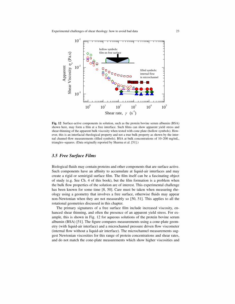
Fig. 12 Surface-active components in solution, such as the protein bovine serum albumin (BSA)shown here, may form a film at a free interface. Such films can show apparent yield stress andshear-thinning of the apparent bulk viscosity when tested with cone plate (hollow symbols). How-ever, this is an interfacial rheological property and not a true bulk property as shown by the inter-nal channel-flow measurements (filled symbols). BSA at bulk concentrations of 10–200 mg/mL,triangles–squares. (Data originally reported by Sharma et al. [51].)

3.5 Free Surface Films

Biological fluids may contain proteins and other components that are surface active.Such components have an affinity to accumulate at liquid-air interfaces and maycreate a rigid or semirigid surface film. The film itself can be a fascinating objectof study (e.g. See Ch. 4 of this book), but the film formation is a problem whenthe bulk flow properties of the solution are of interest. This experimental challengehas been known for some time [8, 50]. Care must be taken when measuring rhe-ology using a geometry that involves a free surface, otherwise fluids may appearnon-Newtonian when they are not measurably so [50, 51]. This applies to all therotational geometries discussed in this chapter.

The primary signatures of a free surface film include increased viscosity, en-hanced shear thinning, and often the presence of an apparent yield stress. For ex-ample, this is shown in Fig. 12 for aqueous solutions of the protein bovine serumalbumin (BSA) [51]. The figure compares measurements using a cone-plate geom-etry (with liquid-air interface) and a microchannel pressure driven flow viscometer(internal flow without a liquid-air interface). The microchannel measurements sug-gest Newtonian viscosities for this range of protein concentrations and shear rates,and do not match the cone-plate measurements which show higher viscosities and


1 0 - 6 1 0 - 5 1 0 - 4 1 0 - 3 1 0 - 2 1 0 - 1 1 0 0 1 0 1 1 0 2 1 0 31

1 0

1 0 0G a p h e i g h t

1 0 5 0 µm 7 0 0 µm 4 5 0 µm

S u r f a c e

s a n d p a p e rs m o o t h

d e c r e a s i n g g a p( s l i p i n d i c a t e d b y l a c k o f o v e r l a p )

Appar

ent str

ess (P

a)

A p p a r e n t s h e a r r a t e ( s - 1 )

Fig. 13 Slip behavior on a smooth geometry surface can decrease flow stress and cause incon-sistent gap-dependence, as shown here for Nivea Lotion tested with different surfaces and gapsusing parallel disks of diameter D = 40 mm. A sandpaper surface eliminates slip artifacts, showingsuperposed data for different gap heights. (Previously unpublished work of author RHE.)

shear-thinning at low rates. The increased viscosity and shear thinning is caused bya free surface film of the BSA [51]. A film is undesirable when measuring bulk prop-erties. Of course, the presence of a film does provide an opportunity for interfacialsurface rheology measurements if this is desired.

Internal flow geometries and guard rings (which eliminate the interface) canavoid the problem (although even in a closed system, there is the possibility ofbiofilm formation in biological fluids). When these are not available or possible,then one must be mindful of the symptoms of a free surface film. To test for the arti-fact of surface film rheology, one could make repeated measurements with differentgeometries and check for reproducibility of apparent material functions. For exam-ple, cones with increasing diameters could be used. The larger diameters create alonger film length and larger moment arm to produce torque and would generallybe expected to have increased torque effects due to free surface films.

3.6 Slip

In rheological characterization, it is typically assumed that the sample sticks to thecontacting boundaries whose motion defines the assumed strain field. In fluids, this


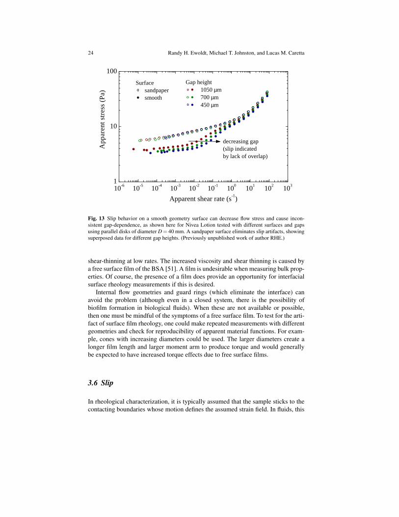
is known as the no-slip condition. However, slip can easily occur [52, 53, 54], es-pecially with biological gels and tissues. Slip violates the assumptions of standardrheological characterization and may cause significant artifacts in the data. Thissection describes slip artifacts, methods of checking for slip, and techniques foravoiding the problem altogether.

The key signatures of slip include a decreased flow stress and inconsistent ap-parent stress and strain rate that depend on the geometry gap (gap height withparallel disks or cone angle with cone-plate). Figure 13 demonstrates these slipartifacts as seen with a non-Newtonian fluid (Nivea Lotion). The smooth bound-ary geometry produces artifacts and the true material behavior can be seen witha roughened surface. The steady state flow sweep is conducted from high to lowrates using a combined motor-transducer rotational rheometer (AR-G2, TA Instru-ments) with a parallel disk of diameter D = 40 mm and controlling temperature toT = 23C with a Peltier plate. The sandpaper surfaces are adhesive-back sandpaper,600 grit (McMaster-Carr Part #47185A51) attached to the standard rheometer ge-ometry on both bounding surfaces. Apparent shear stress is calculated as τa = Fτ Twith Fτ = 2/(πR3) for the disk, and apparent shear rate from γa = Ω/h where h isthe geometry gap.

Figure 13 shows an apparent stress plateau at low rates (an apparent dynamicyield stress) that depends on the geometry being used. The smooth geometry showsa lower apparent yield stress. This is a common experimental artifact that has beendiscussed in the literature, especially with yield stress fluids [55, 56]. In a recentstudy with a dense colloidal system, apparent yield stress behavior at low rates wasassociated with a sub-colloidal lubrication layer at the wall, as confirmed by confo-cal microscopy [56].

The gap is varied to check for slip in Fig. 13. For the rough sandpaper surface,the measurements superpose for all gaps therefore confirming the absence of slip.However, for the smooth plate, the data shifts to higher apparent strain rate as thegap is decreased. This shift is important evidence to indicate slip. To understandwhy, consider the simple example where an applied stress results in a particular slipvelocity at the boundary of a sample. The gap-independent slip velocity contributesa fixed amount to the total velocity Ω . Therefore, as the gap h decreases, the ap-parent shear rate γa = Ω/h will have a numerator that decreases slower than thedenominator, therefore increasing γa at small gaps for a fixed stress. This is shownby the arrow in Fig. 13 pointing to the right. Varying the geometry checks for thepresence of slip, but can also be used to correct for slip [57]. With very good controland sensitive instruments, gap-dependent measurements with a linear sliding platerheometer have been used to characterize the slip itself including slip velocities [58].

Although sandpaper may be sufficient for some biological gels, e.g. as usedfor biopolymer mucin gels (snail slime) [59], sandpaper roughness is not alwayssufficient and other techniques must be considered. This includes the addition ofgrooves [55] or “cleats” [60] in plates, e.g. as used to measure vitreous humor [61].Vane rotors are also commonly available [62], which are modifications of the con-centric cylinder geometry. For more challenging solid materials, such as soft bio-logical tissues, the sample can be squeezed slightly with an applied normal load


1 0 1 1 0 2 1 0 3 1 0 4 1 0 5 1 0 61 0 - 1

1 0 0

1 0 1

R e= 4

( h =1 0 0

µ m)

s e co n d

a r y f l o

w li m i

tR e

= 4 ( h =

5 0 0µ m

)

A p p a r e n tg a p h e i g h t , h a

5 0 0 µm 4 0 0 µm 3 0 0 µm 2 5 0 µm 2 0 0 µm 1 5 0 µm 1 0 0 µm 7 5 µm 5 5 µm 4 5 µm 3 5 µm 2 5 µm 1 5 µm 1 0 µm

Appar

ent Vi

scosity

, a [m

Pa.s]

S h e a r R a t e , γ [ s - 1 ]

i n c r e a s i n g g a p :s e c o n d a r y f l o w

d e c r e a s i n g g a p :o f f s e t e r r o r

l o w - t o r q u el i m i t

h

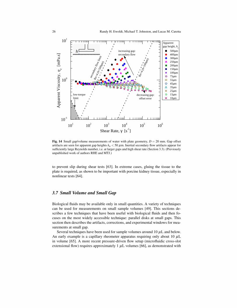
Fig. 14 Small gap/volume measurements of water with plate geometry, D = 20 mm. Gap offsetartifacts are seen for apparent gap heights ha < 50 µm. Inertial secondary flow artifacts appear forsufficiently large Reynolds number, i.e. at larger gaps and high shear rate (Section 3.3). (Previouslyunpublished work of authors RHE and MTJ.)

to prevent slip during shear tests [63]. In extreme cases, gluing the tissue to theplate is required, as shown to be important with porcine kidney tissue, especially innonlinear tests [64].

3.7 Small Volume and Small Gap

Biological fluids may be available only in small quantities. A variety of techniquescan be used for measurements on small sample volumes [49]. This sections de-scribes a few techniques that have been useful with biological fluids and then fo-cuses on the most widely accessible technique: parallel disks at small gaps. Thissection then describes the artifacts, corrections, and experimental windows for mea-surements at small gap.

Several techniques have been used for sample volumes around 10 µL and below.An early example is a capillary rheometer apparatus requiring only about 10 µLin volume [65]. A more recent pressure-driven flow setup (microfluidic cross-slotextensional flow) requires approximately 1 µL volumes [66], as demonstrated with


1 0 - 2 1 0 - 1 1 0 0 1 0 1 1 0 2 1 0 31 0 0

1 0 1

1 0 2

1 0 3

( v ) s m a l l g a p l i m i t

( i i i ) s e c o n d a r y f l o w l i m i t

( i v ) m a x i m u m v o l u m e l i m i t

Gap,

h [µm

]

V e l o c i t y , [ r a d / s ]

E x p e r i m e n t a lW i n d o w

( i i ) m a x v e l o c i t y l i m i t

( i ) lo w - t o r

q u e l i m

i t

Fig. 15 Experimental window for small volume aqueous solutions, using Eqs. 34–38 to draw theboundaries. Representative values used are Tmin = 5 nN.m, Ωmax = 300rad/s, Remax = 4, η =1 mPa.s, ρ = 1000 kg/m3, plate diameter D = 8 mm, Vmax = µL, and minimum gap hmin = 10 µm.

hyaluronic acid and saliva. Boundary driven flow examples include modificationof parallel disks to confine a sample near the outer radius over a small area, ap-proximating sliding plate flow with volumes 1–25 µL [48]. A custom-built linearsliding plate instrument has also been developed for precise, small gap tests (the so-called flexure-based microgap rheometer (FMR) [67, 68]). The FMR has been usedto measure microliter quantities of spider silk [69] and sub-microliter quantities ofcarnivorous plant mucilage [70]. In those studies, samples were also tested with asmall-scale extensional instrument based on capillary-breakup extensional rheom-etry (CaBER). Embedded probe techniques are also useful. Nanoliter droplets ofbutterfly saliva have been characterized with an embedded magnetic rod [71]. Ofall the demonstrated techniques, standard parallel disks at small gaps may be themost experimentally accessible option for a researcher interested in small volumesof biological fluid.

With parallel disks, the smallest accessible gap will be limited by disk paral-lelism, precise knowledge of the true gap, and the size of the underlying materialstructure in the fluid. Confinement effects that violate the continuum hypothesis will


not be discussed here (although this is sometimes relevant in biological fluids, suchas blood exhibiting a confinement-dependent viscosity [72]). Finite boundary rough-ness and tribological contact will not be discussed either, since other gap errors aretypically encountered first. Gap errors, including parallelism and gap precision, arethe primary concern, assuming the continuum hypothesis holds true.

For gap errors, measurement artifacts include a decreasing apparent viscosity atsmaller gaps (Fig. 14). This occurs under the typical scenario where the true gap his larger than the apparent gap ha calibrated by apparent contact of the plates [73].These symptoms and limitations apply similarly to any boundary driven drag flow atsmall gaps, such as the sliding plate FMR [67, 67] and techniques to isolate samplesto a small region under a conventional parallel disk geometry [48], although thedifference between h and ha may change depending on the calibration procedure.

Fig. 14 shows the expected artifacts for small gap measurements, here with waterusing a disk with diameter D = 20 mm down to apparent gap ha = 10 µm (down toapparent volume around 3 µL). Using small gaps requires less volume and allowsfor higher shear rates. On average, the viscosity is what we expect for water, η ≈1 mPa.s, but there are some issues. For small gaps (ha < 50 µm), the apparentviscosity decreases as a function of gap. For the larger gaps (ha ≥ 100 µm), theviscosity seems to shear-thicken at high shear rates, but at different critical shearrates. These are not true material properties of water, but are artifacts that can beexplained.

For larger gaps at high rates, the inertia of the liquid may cause secondary flows(as described in Section 3.3). It is common to assume that the liquids will travelin circular stream lines, but centrifugal effects will tend to push fluid outward neara rotating boundary. This secondary flow increases dissipation, resulting in highermeasured torque and hence a larger apparent viscosity. The effect increases as afunction of Reynolds number, defined as Re = ρΩh2/η , so the effect is evidentfor higher velocity Ω , larger gaps h, and low viscosity fluids. Lines for Re = 4 areshown in the figure for two representative gap heights.

For small gaps, the main error is caused by a gap offset εh, which is the differencebetween the apparent calibrated gap ha and true gap h [73],

h = ha + εh. (32)

(The term “true” gap means the “effective” or “average” gap since the disks havefinite roughness and finite parallelism manufacturing tolerance. Hence the gap is notprecisely constant throughout the test geometry.) Since apparent gap ha is used tocalculate apparent viscosity ηa, one expects deviation from the the true viscosity tobe of the form

ηa = ηha

h(33)

which indicates ηa < η for offset εh > 0. The apparent gap ha is typically calibratedbased on contact force at the first point of contact, where ha is set to zero. Twoissues arise to create gap offset error εh > 0. (i) A finite force is often observedbefore solid-solid contact due to viscous resistance of air flow in the squeezing gap.


(ii) The parallelism is not perfect, and the average gap will often be larger thanthe “first point of contact” gap. The non-parallelism contribution generates normalforces [74] and this can be used to identify the relative importance of the two sourcesof gap offset error. Both of these effects contribute to gap offset error εh > 0, so thatthe actual gap is larger than the apparent value. Typical values for εh are on the orderof 10–50µm [75, 76].

Gap offset εh can be corrected if Eq. 33 holds true [73, 75, 76], although thecorrection will depend on the uncertainty in calibrating for εh. Uncertainly in thecalculated viscosity will grow dramatically as the gap approaches the uncertaintyof εh. Gap offset errors can be minimized by using a smaller radius plate, sincethis decreases the viscous squeeze force at apparent contact and also decreases thenon-parallelism (angular misalignment) contribution to εh due to the smaller radius.However, a smaller radius plate changes other experimental limits such as increasingηmin due to the low-torque limit (Eq. 13). The experimental window for small gapmeasurements is therefore bounded by several limitations.

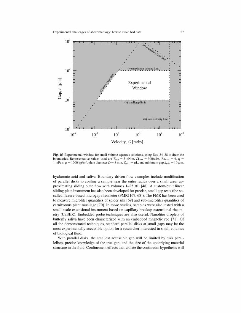
Figure 15 is an example experimental window for small volume and small gapmeasurements, in the operational space of gap h and velocity Ω . Several limitationsare considered including (i) minimum torque, (ii) maximum velocity, (iii) secondaryflow, (iv) maximum volume available, and (v) small gap limit, e.g. due to gap offseterrors. The exact locations of the boundaries will shift depending on the fluid prop-erties and instrument used, but their shapes will not change. Representative valuesare used in Fig. 15 for aqueous fluids. Specific equations for boundary lines comefrom consideration of each limit. The minimum torque, item (i), is set either bythe instrument specification (Section 3.1) or surface tension torque which becomesincreasingly important at small gaps (Section 3.4). Based on the criteria T > Tmin,where torque from steady viscosity is T = (ηΩ/h)/Fτ , the boundary line is definedby

h <ηΩ

Fτ Tmin(34)

which shows the scaling h ∼ Ω that appears in Fig. 15. The instrument limit ofmaximum velocity, item (ii), is simply set by the criteria

Ω < Ωmax (35)

and therefore appears as a vertical line in the figure. The limit of secondary flow,item (iii), was discussed in Section 3.3. There, a maximum Reynolds number Remax

sets the boundary line, and is based on the definition Re= ρΩh2

ηfor parallel disks.

Then, the criteria Re< Remax can be written

h <

(Remaxη

ρΩ

)1/2

(36)

which shows the scaling h ∼ Ω−1/2 seen in the top right of Fig. 15. The last twocriteria come from this section, considering small volume and small gap limitations.The volume limit is simply V < Vmax where Vmax is the maximum sample volume


available. For parallel disks, V = πR2h, and the boundary line is defined by

h <Vmax

πR2 . (37)

The final boundary, item (v), is the minimum gap. This boundary line is defined by

h > hmin (38)

where hmin is set by the gap offset error, or possibly the minimum gap where con-finement effects are negligible and the material can still be considered a continuum.Figure 15 uses Eqs. 34–38 with representative parameters given in the caption. Theminimum gap h = 10 µm is used, assuming uncertainty in gap error much less than10 µm which would allow for gap offset corrections. Based on the maximum sam-ple volume and minimum gap limits, the experimental window is confined betweenh = 10−100 µm for this example. If larger volumes are available, then larger gapscan be used, eventually being limited by the secondary flow (e.g. as seen in Fig. 14at larger gaps). At very large gaps, the experimental window vanishes. This oc-curs where the minimum torque and secondary flow boundaries intersect, for gapsh > 1000 µm with this particular geometry.

3.8 Other Issues

Additional challenges, basic and exotic, can also be included on the list of possibleways that rheological measurements can go astray.

One basic but important point is sample volume underfill or overfill. In cone-plateand parallel disk geometries, torque is a very sensitive function of the radial extentof contact T ∼ 1

R3 [8]. Underfill is more sensitive than overfill, but for both cases onemay have the problem of an uncontrolled contact line that loses rotational symmetrywhich can introduce additional torque due to surface tension forces (Section 3.4).Underfill can also develop as a sample evaporates. This is relevant to aqueous bio-logical fluids. Evaporation can be eliminated or reduced by the use of a solvent trap.The use of a micropipette and close attention to fill level can further eliminate thebasic issue of sample volume underfill or overfill.

An exotic but relevant issue with some biological fluids is particle settling andmigration, in particular with active-swimming microorganisms in suspension. Ingeneral, the concentric cylinder geometry is recommended when gravitational parti-cle settling may be an issue, since a depletion layer is not created across the velocitygradient direction as would be the case with cone-plate or parallel disk geometries.But, if the sample volume is not sufficient, parallel disks or the cone-plate geometrymust be used. One particularly striking example is with the same microalgae sus-pension whose flow data is given in Fig. 3. Those measurements were made with acone-plate geometry. The data needed to be collected within the first two minutesof flow due to microalgae rheotaxis (flow-induced swimming), coupled with parti-


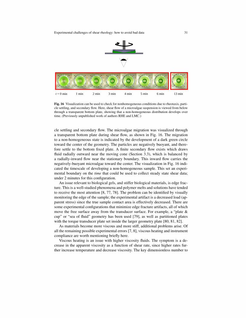
t = 0 min 1 min 2 min 3 min 4 min 5 min 6 min 13 min

Fig. 16 Visualization can be used to check for nonhomogeneous conditions due to rheotaxis, parti-cle settling, and secondary flow. Here, shear flow of a microalgae suspension is viewed from belowthrough a transparent bottom plate, showing that a non-homogeneous distribution develops overtime. (Previously unpublished work of authors RHE and LMC.)

cle settling and secondary flow. The microalgae migration was visualized througha transparent bottom plate during shear flow, as shown in Fig. 16. The migrationto a non-homogeneous state is indicated by the development of a dark green circletoward the center of the geometry. The particles are negatively buoyant, and there-fore settle to the bottom fixed plate. A finite secondary flow exists which drawsfluid radially outward near the moving cone (Section 3.3), which is balanced bya radially-inward flow near the stationary boundary. This inward flow carries thenegatively-buoyant microalgae toward the center. The visualization in Fig. 16 indi-cated the timescale of developing a non-homogeneous sample. This set an experi-mental boundary on the time that could be used to collect steady state shear data;under 2 minutes for this configuration.

An issue relevant to biological gels, and stiffer biological materials, is edge frac-ture. This is a well-studied phenomena and polymer melts and solutions have tendedto receive the most attention [8, 77, 78]. The problem can be identified by visuallymonitoring the edge of the sample; the experimental artifact is a decreased load (ap-parent stress) since the true sample contact area is effectively decreased. There aresome experimental configurations that minimize edge fracture artifacts, all of whichmove the free surface away from the transducer surface. For example, a “plate &cup” or “sea of fluid” geometry has been used [79], as well as partitioned plateswith the torque transducer plate set inside the larger geometry plate [80, 81, 82].

As materials become more viscous and more stiff, additional problems arise. Ofall the remaining possible experimental errors [7, 8], viscous heating and instrumentcompliance are worth mentioning briefly here.

Viscous heating is an issue with higher viscosity fluids. The symptom is a de-crease in the apparent viscosity as a function of shear rate, since higher rates fur-ther increase temperature and decrease viscosity. The key dimensionless number to


check is the Nahme number [2], which can be interpreted as a ratio of viscositychange due to viscous heating compared to the baseline viscosity. Values near zeroindicate negligible viscosity change. Smaller gaps help minimize the heating effect,since they decrease the length of the thermal conduction path. This is most impor-tant for liquids with high viscosity and low thermal conductivity. For low-viscositybiological fluids, this is less of an issue.

System compliance is an issue with higher stiffness materials. The problem liesin the possibility of finite movement of a “fixed” boundary due to system compli-ance, or small but finite movement of the load cell, even with modern force rebal-ancing transducers [83, 84]. Instrument compliance issues have been identified withthe dynamic shear measurement of glycerol [85] and polymer melts [86]. Recom-mendations have been identified for experimental protocol and instrument designto avoid, minimize, and correct for compliance effects [87]. Instrument complianceerrors should be considered for stiff, solid materials, or the short time data from stepstrain inputs when material stiffness may also be large.

4 Conclusions

The experimental challenges described here will serve as a checklist for trou-bleshooting and debugging rheological measurements of complex fluids. Thesechallenges are especially evident with biofluids and biological materials. Commonartifacts cause a fluid to inaccurately appear as shear-thinning, shear-thickening,having frequency-dependence, time-dependence, or having an elastic modulus,when these behaviors are not actually present in the true intensive material response.

We encourage the reader to think critically about experimental rheological mea-surements, and to ask appropriate and fair questions about the validity of data (in-cluding their own and those published in the open literature). This is particularlyrelevant for biological complex fluids which are soft, have low viscosity, and maycontain active components.

For each potential artifact, the system-level perspective can identify an experi-mental boundary and/or a method of minimizing the effect (Sections 3.1–3.8). Thefocus here has been on the most commonly used technique for measuring shear ma-terial functions, i.e. drag flow at the boundary ([8] Ch.5), especially when imposedby rotational geometries such as parallel disks, cone-plate, or concentric cylinders(Figure 1). Other measurement techniques, including those described in this book(Ch.1, 3-5), will also benefit from a system-level perspective that acknowledges non-ideal conditions for rheological material function measurement (as in Figure 1). Theidentification of experimental boundaries (similar to Figures 3, 6, 5, 10, 11, 14, and15) will be especially relevant to biological fluids and materials that are of limitedvolume, as well as soft, active, and rheologically-complex materials more generally.

Acknowledgements This work was supported by the National Science Foundation under GrantNo. CBET-1342408. RHE and LMC acknowledge helpful discussions regarding careful rheologi-


cal measurements with Prof. Christopher Macosko and Dr. David Giles at the University of Min-nesota. RHE also thanks Prof. Gareth McKinley at the Massachusetts Institute of Technology forinitial discussions on drawing experimental boundaries for rheological measurements. RHE andLMC also acknowledge Prof. Jian Sheng at Texas Tech University (formerly University of Min-nesota) for suggesting the study of actively-swimming microalgae suspensions, and Mr. AnwarChengala for preparing those samples.

Appendix: Material details - hagfish gel and microalgaesuspension

Hagfish gel serves as an example of an ultrasoft biomaterial gel. It is prepared asin [5, 14] and used in Figs. 5–7.

The actively-swimming microalgae suspension provides an example of a low vis-cosity biological solution and is used in Figs. 3 and 16. The algal species Dunaliellaprimolecta was used. It is a motile, bi-flagellated, cell-wall-less, unicellular greenalgae that does not clump. It has slight negative buoyancy, a approximate charac-teristic diameter 11 µm, and natural concentration on the order of 3 ·106 cells/mL.Dunaliella Primolecta (UTEX LB 1000) was obtained from UTEX, The CultureCollection of Algae at the University of Texas at Austin. Non-motile samples wereprepared by adding 2mL of 4 %wt/vol of formaldehyde in Phosphate BufferedSaline (PBS) solution to 25mL of the bulk sample. The fixed sample was analyzedunder light microscope to ensure it was non-motile.

References

1. Dealy, J. M. Journal of Rheology 39(1), 253–265 (1995).2. Bird, R. B., Curtiss, C. F., Armstrong, R. C., and Hassager, O. Dynamics of Polymeric Liquids:

Volume 2 Kinetic Theory, volume 2nd. John Wiley and Sons, Inc, New York, (1987).3. Larson, R. G. The structure and rheology of complex fluids. Oxford University Press, New

York, (1999).4. Bharadwaj, N., Allison, J. T., and Ewoldt, R. H. In ASME 2013 International Design En-

gineering Technical Conferences & Computers and Information in Engineering Conference,paper DETC2013–13462 (, Portland, OR, 2013).

5. Ewoldt, R. H., Winegard, T. M., and Fudge, D. S. International Journal of Non-Linear Me-chanics 46(4), 627–636 (2011).

6. Ewoldt, R. H. Journal of Rheology 57(1), 177–195 (2013).7. Walters, K. Rheometry. Wiley, New York, (1975).8. Macosko, C. W. Rheology: principles, measurements, and applications. Wiley-VCH, New

York, (1994).9. Powell, R. L. In Rheological Measurement, Collyer, A. A. and Clegg, D. W., editors, chapter 9,

260–298. Springer Netherlands, Dordrecht2nd edition (1998).10. Oliveira, M. S., Yeh, R., and McKinley, G. H. Journal of Non-Newtonian Fluid Mechanics

137(1-3), 137–148 August (2006).11. Rodd, L. E., Scott, T. P., Boger, D. V., Cooper-White, J. J., and McKinley, G. H. Journal of

Non-Newtonian Fluid Mechanics 129(1), 1–22 August (2005).


12. Soulages, J., Oliveira, M., Sousa, P., Alves, M., and McKinley, G. Journal of Non-NewtonianFluid Mechanics 163(1-3), 9–24 November (2009).

13. Johnston, M. and Ewoldt, R. Journal of Rheology 57(6), 1515–1532 (2013).14. Fudge, D. S., Winegard, T., Ewoldt, R. H., Beriault, D., Szewciw, L., and McKinley, G. H.

Integrative and Comparative Biology 49(1), 32–39 (2009).15. Baravian, C. and Quemada, D. Rheologica Acta 37(3), 223–233 June (1998).16. Baravian, C., Benbelkacem, G., and Caton, F. Rheologica Acta 46(5), 577–581 November

(2006).17. Ewoldt, R. H. and McKinley, G. H. Rheology Bulletin 76(1), 4 (2007).18. Yao, N. Y., Larsen, R. J., and Weitz, D. A. Journal of Rheology 52(4), 1013–1025 (2008).19. Lin, Y.-C., Koenderink, G. H., MacKintosh, F. C., and Weitz, D. A. Macromolecules 40(21),

7714–7720 October (2007).20. Sharif-Kashani, P., Hubschman, J.-P., Sassoon, D., and Kavehpour, H. P. Journal of biome-

chanics 44(3), 419–23 February (2011).21. Broedersz, C. P., Kasza, K. E., Jawerth, L. M., Munster, S., Weitz, D. A., and MacKintosh,

F. C. Soft Matter 6(17), 4120 August (2010).22. Lee, H., Ferrer, J. M., Nakamura, F., Lang, M. J., and Kamm, R. D. Acta biomaterialia 6(4),

1207–18 April (2010).23. Weigandt, K. M., Pozzo, D. C., and Porcar, L. Soft Matter 5(21), 4321 October (2009).24. Suri, S. and Schmidt, C. E. Acta biomaterialia 5(7), 2385–97 September (2009).25. Struik, L. C. E. Rheologica Acta 6(2), 119–129 May (1967).26. Mackay, M. E., Liang, C. H., and Halley, P. J. Rheologica Acta 31(5), 481–489 (1992).27. Magda, J. and Larson, R. Journal of Non-Newtonian Fluid Mechanics 30(1), 1–19 October

(1988).28. Shaqfeh, E. S. G. Annual Review of Fluid Mechanics 28, 129–185 November (1996).29. McKinley, G. H., Pakdel, P., and Oztekin, A. Journal of Non-Newtonian Fluid Mechanics 67,

19–47 November (1996).30. Pakdel, P. and McKinley, G. Physical Review Letters 77(12), 2459–2462 September (1996).31. Schrag, J. L. Journal of Rheology 21(3), 399 September (1977).32. Yosick, J. A., Giacomin, J. A., Stewart, W. E., and Ding, F. Rheologica Acta 37(4), 365–373

(1998).33. Storm, C., Pastore, J. J., MacKintosh, F. C., Lubensky, T. C., and Janmey, P. A. Nature

435(7039), 191–194 May (2005).34. Taylor, G. I. Philosophical Transactions of the Royal Society of London. Series A, Containing

Papers of a Mathematical or Physical Character 223(605-615), 289–343 January (1923).35. Chandrasekhar, S. Hydrodynamic and hydromagnetic stability. Dover, New York, (1981).36. Larson, R. G. Rheologica Acta 31(3), 213–263 (1992).37. ISO. 3219, Determination of viscosity using a rotational viscometer with defined shear rate

(1993).38. Sdougos, H. P., Bussolari, S. R., and Dewey, C. F. Journal of Fluid Mechanics 138, 379–404

(1984).39. Turian, R. M. Industrial & Engineering Chemistry Fundamentals 11(3), 361–368 August

(1972).40. Meulenbroek, B., Storm, C., Morozov, A. N., and van Saarloos, W. Journal of Non-Newtonian

Fluid Mechanics 116(2-3), 235–268 January (2004).41. Pan, L., Morozov, A., Wagner, C., and Arratia, P. E. Physical Review Letters 110(17), 174502

April (2013).42. Griffiths, D. F. and Walters, K. Journal of Fluid Mechanics 42(02), 379–399 March (1970).43. Shipman, R. W. G., Denn, M. M., and Keunings, R. Industrial & Engineering Chemistry

Research 30(5), 918–922 (1991).44. Orr, F. M., Scriven, L. E., and Rivas, A. P. Journal of Fluid Mechanics 67(04), 723–742 March

(1975).45. Fortes, M. A. Journal of Colloid and Interface Science 88(2), 338–352 (1982).46. De Souza, E. J., Gao, L., McCarthy, T. J., Arzt, E., and Crosby, A. J. Langmuir 24(4), 1391–6

March (2008).


47. Laun, H. M. and Meissner, J. Rheologica Acta 19(1), 60–67 January (1980).48. Mackay, M. E. and Cathey, C. A. Journal of Rheology 35(2), 237 February (1991).49. Mackay, M. E. In Rheological Measurement, Collyer, A. and Clegg, D., editors, chapter 20,

635–665. Springer Netherlands2nd edition (1998).50. Merrill, E. Physiological Reviews 49(4), 863–888 (1969).51. Sharma, V., Jaishankar, A., Wang, Y.-C., and McKinley, G. H. Soft Matter 7(11), 5150 (2011).52. Buscall, R., McGowan, J. I., and Morton-Jones, A. J. Journal of Rheology 37(4), 621–641

July (1993).53. Barnes, H. A. Journal of Non-Newtonian Fluid Mechanics 56(3), 221–251 March (1995).54. Buscall, R. Journal of Rheology 54(6), 1177–1183 October (2010).55. Magnin, A. and Piau, J. Journal of Non-Newtonian Fluid Mechanics 36, 85–108 December

(1990).56. Ballesta, P., Petekidis, G., Isa, L., Poon, W. C. K., and Besseling, R. Journal of Rheology

56(5), 1005–1037 June (2012).57. Yoshimura, A. and Prudhomme, R. K. Journal of Rheology 32(1), 53–67 January (1988).58. Clasen, C. Rheologica Acta 51(10), 883–890 August (2012).59. Ewoldt, R. H., Clasen, C., Hosoi, A. E., and McKinley, G. H. Soft Matter 3(5), 634–643

(2007).60. Nickerson, C. S. and Kornfield, J. A. Journal of Rheology 49(4), 865 July (2005).61. Nickerson, C. S., Park, J., Kornfield, J. A., and Karageozian, H. Journal of biomechanics

41(9), 1840–6 January (2008).62. Barnes, H. A. and Nguyen, Q. D. Journal of Non-Newtonian Fluid Mechanics 98(1), 1–14

March (2001).63. Tan, K., Cheng, S., Juge, L., and Bilston, L. E. Journal of biomechanics 46(6), 1060–6 April

(2013).64. Nicolle, S. and Palierne, J.-F. Journal of the mechanical behavior of biomedical materials

14(null), 158–62 October (2012).65. Philippoff, W., Han, C., Barnett, B., and Dulfano, M. Biorheology 7(1), 55–67 (1970).66. Haward, S. J., Sharma, V., and Odell, J. A. Soft Matter 7(21), 9908 October (2011).67. Clasen, C. and McKinley, G. H. Journal of Non-Newtonian Fluid Mechanics 124(1-3), 1–10

December (2004).68. Clasen, C., Gearing, B. P., and McKinley, G. H. Journal of Rheology 50(6), 883–905 (2006).69. Kojic, N., Bico, J., Clasen, C., and McKinley, G. H. The Journal of experimental biology

209(Pt 21), 4355–62 November (2006).70. Erni, P., Varagnat, M., Clasen, C., Crest, J., and McKinley, G. H. Soft Matter 7(22), 10889

November (2011).71. Tokarev, A., Kaufman, B., Gu, Y., Andrukh, T., Adler, P. H., and Kornev, K. G. Applied

Physics Letters 102(3), 033701 January (2013).72. Fa hræus, R. and Lindqvist, T. American Journal of Physiology 96(3), 562–568 March (1931).73. Connelly, R. W. and Greener, J. Journal of Rheology 29(2), 209 April (1985).74. Andablo-Reyes, E., Hidalgo-Alvarez, R., and de Vicente, J. Journal of Non-Newtonian Fluid

Mechanics 165(19-20), 1419–1421 October (2010).75. Davies, G. A. and Stokes, J. R. Journal of Rheology 49(4), 919–922 (2005).76. Pipe, C. J., Majmudar, T. S., and McKinley, G. H. Rheologica Acta 47(5-6), 621–642 April

(2008).77. Tanner, R. I. and Keentok, M. Journal of Rheology 27(1), 47 February (1983).78. Keentok, M. and Xue, S.-C. Rheologica Acta 38(4), 321–348 October (1999).79. Vrentas, J. S., Venerus, D. C., and Vrentas, C. M. Journal of Non-Newtonian Fluid Mechanics

40(1), 1–24 July (1991).80. Schweizer, T. Journal of Rheology 47(4), 1071 June (2003).81. Wang, S.-Q., Ravindranath, S., and Boukany, P. E. Macromolecules 44(2), 183–190 (2011).82. Snijkers, F. and Vlassopoulos, D. Journal of Rheology 55(6), 1167 August (2011).83. Mackay, M. E. and Halley, P. Journal of Rheology 35(8), 1609 November (1991).84. Liu, C.-Y., Yao, M., Garritano, R. G., Franck, A. J., and Bailly, C. Rheologica Acta 50(5-6),

537–546 June (2011).


85. Schroter, K., Hutcheson, S. A., Shi, X., Mandanici, A., and McKenna, G. B. The Journal ofchemical physics 125(21), 214507 December (2006).

86. Schweizer, T. and Bardow, A. Rheologica Acta 45(4), 393–402 March (2006).87. Hutcheson, S. A. and McKenna, G. B. The Journal of chemical physics 129(7), 074502 August

(2008).

Documents

Experimental challenges of shear rheology: how to avoid ... · Experimental challenges of shear rheology: how to avoid bad data Randy H. Ewoldt, Michael T. Johnston, and Lucas M