EXPERIMENTAL AND NUMERICAL INVESTIGATION OF … · EXPERIMENTAL AND NUMERICAL INVESTIGATION OF A MICRO ... The bubble cutting generates smaller bubbles ... sure and record local pH

Eleventh International Conference on CFD in the Minerals and Process IndustriesCSIRO, Melbourne, Australia7-9 December 2015

EXPERIMENTAL AND NUMERICAL INVESTIGATION OF A MICRO-STRUCTUREDBUBBLE COLUMN WITH CHEMISORPTION

Krushnathej THIRUVALLUVAN SUJATHA1∗, Deepak JAIN1†, Satish KAMATH1‡, J. A. M.

KUIPERS1§, Niels G. DEEN1¶

1Department of Chemical Engineering and Chemistry, Eindhoven University of Technology, P.O. Box

513, 5600MB Eindhoven, The Netherlands

∗ E-mail: [email protected]† E-mail: [email protected]

‡ E-mail: [email protected]§ E-mail: [email protected]

¶ E-mail: [email protected]

ABSTRACTBubble columns reactors are often used for gas-liquid contactingprocesses, for instance in gas-treating processes for H2S and/orCO2 removal. The limiting step in the chemisorption process isusually the mass transfer from the gas phase to the liquid phase.The mass transfer rate is a function of the interfacial area, theintrinsic mass transfer coefficient and the driving force. Themass transfer rate can be increased by increasing the interfacialarea and/or the interfacial mass transfer coefficient. This canbe achieved by means of adding internals such as sieve plates,porous plates, and static mixers (SMV). The addition of internalsis also known to reduce the back-mixing in bubble column reac-tors, which can be advantageous in some situations. In this work,the internals are wire-meshes and serve the purpose of cutting thebubbles. The bubble cutting generates smaller bubbles leading toan increase in gas-liquid interfacial area.

In our previous work, three hydrodynamic regimes were identi-fied for bubbly flow in a micro-structured bubble column (MSBC)with wire mesh (Sujatha et al., 2015). These studies were per-formed for an air-water system with superficial gas velocitiesranging from 5 to 50 mm/s. The effect of the wire mesh lay-outs on bubble cutting was studied for the case without physicalabsorption/reaction. The scope of the current research is to ex-tend the work for the case of chemisorption of CO2 into a NaOHsolution, by a combined experimental and simulation approach.Bubble size distribution, pH and holdup data are obtained fromchemisorption experiments. These data are compared with sim-ulation results obtained from a detailed VOF-DBM model devel-oped by Jain et al. (2014).

Keywords: Micro-Structured Bubble Column, Digital ImageAnalysis, CO2 – NaOH system, wire mesh, pH measurement .

NOMENCLATURE

Greek Symbolsε Gas holdup, [-].µ Dynamic viscosity, [kg/ms].σ Surface tension, [-].ρ Density, [kg/m3].

Latin Symbolsd Diameter, [m].W Width, [m].H Height, [m].

D Depth, [m].A Area, [m2].V Volume, [m3].h height of liquid-gas dispersion, [m2].u Velocity, [m/s].Sh Sherwood number, [-].Re Reynolds number, [-].Sc Schmidt number, [-].

Sub/superscriptseq Equivalent.b Bubble.g Gas.l Liquid.f Fluid.w Wire.k Index k.H height expansion.DIA Digital Image Analysis.F Final.0 Initial.

INTRODUCTION

Bubble columns are often used for gas-liquid contactingprocesses, for instance in gas-treating processes for H2Sand/or CO2 removal. The limiting step in the chemisorp-tion process is usually the mass transfer from the gas phaseto the liquid phase. The mass transfer rate is a function ofthe interfacial area, the intrinsic mass transfer coefficientand the driving force. The mass transfer rate can be in-creased by increasing the interfacial area and/or the interfa-cial mass transfer coefficient. This can achieved by meansof adding internals such as sieve plates, porous plates, andstatic mixers (SMV) (Baird, 1992; Deen et al., 2000). Theaddition of internals is also known to reduce the back-mixing in the bubble column reactor, which can be advan-tageous in some situations. In our previous work, we haveproposed a novel micro-structured bubble column(MSBC)reactor with wire-meshes as internals (Sujatha et al., 2015;Jain et al., 2013, 2014). Jain et al. (2013, 2014) have devel-oped a combined VOF-DBM model to simulate and studythe effect of wire mesh in the MSBC reactor. Sujatha et al.(2015) have done experiments in laboratory scale MSBC

Copyright c© CSIRO Australia1

Mesh # diameter (mm) opening (mm) open area (%)4 0.80 5.5 766 0.55 3.6 766 0.90 3.3 628 0.50 2.7 7110 0.31 2.2 7512 0.31 1.8 7318 0.22 1.1 71

Table 1: Overview of different wire meshes used for ex-periments

reactor to study the effect of wire mesh configuration andsuperficial gas velocity. Three hydrodynamic regimes wereidentified for bubbly flow in a MSBC with wire mesh in anair-water system for superficial gas velocities in the rangeof 5 to 50 mm/s.

The scope of the current paper is to extend the work forthe chemisorption of CO2 into a NaOH solution, by acombined experimental and simulation approach. Bubblesize distribution, pH and holdup data are obtained fromchemisorption experiments. These data are compared withsimulation results obtained from a detailed VOF-DBMmodel developed by Jain et al. (2014).

This paper is organized as follows. The description of theexperimental setup and methods used for obtaining the re-sults (i.e. digital image analysis technique and VOF-DBMmethod) are discussed elaborately. The results and discus-sion section consists of visual analysis, experimental re-sults and comparison of experiments with simulation.

MATERIAL AND METHODS

A flat pseudo-2D bubble column reactor of dimensions(width W=0.2 m, depth D=0.03 m, height H=1.3 m) is cho-sen for experiments. The reactor walls are constructed oftransparent glass to enable visual observation by the eye orusing a camera. The gas is fed into the column via a groupof fifteen gas needles centrally arranged in the distributorplate. The needles have a length (L) = 50 mm, inner diam-eter (I.D.) = 1 mm and outer diameter (O.D.) = 1.5875 mm.The needles extend 10 mm above the bottom plate and arespaced with a center-to-center distance of 9 mm. An ar-ray of five needles is classified as a group, and each groupof needles is connected to a mass flow controller. Subse-quently, three mass flow controllers are used to control thegas flow rates in the column. Micro-structuring in the reac-tor is realized by means of thin wires of various dimensionsarranged in a mesh structure or by using a Sulzer packing(SMV). The wire mesh or Sulzer packing can be mountedonto the column by using a modular insert, designed forthis purpose. The modular insert design allows full flexi-bility to attach one or more wire meshes at different loca-tions of the insert. The dimensions of the column includ-ing the insert are as follows: width=0.14 m, depth=0.03 m,height=1.3 m. The location of the wire mesh was fixed forthe experiments at a distance of 0.26 m from the bottomdistributor plate and the Sulzer packing is fixed at 0.24 to0.26 m. An overview of the several mesh configurationscan be seen in Table 1.

The experimental procedure followed for the CO2−NaOH

system is as follows. The column is filled with a wellstirred solution of sodium hydroxide prepared with pH =12.5. Inert gas nitrogen is used to aerate the column beforethe starting time of the experiment at desired gas flow rate.The camera is focused to a particular section of the col-umn to capture sharp images. The pH meter is immersedin the NaOH solution, at the top of the column to mea-sure and record local pH for the duration of reaction. Theflow is switched to CO2 and the timer is started. Initial liq-uid height is noted down at time t = 0 and the high-speedrecording of images is started. As the reaction proceeds thechange in height of gas-liquid dispersion is noted down.Once there is no relevant change in pH with time the CO2flow is switched back to nitrogen flow. The change in thegas holdup is observed via the change in height of the gas-liquid dispersion with time.

Digital Image Analysis

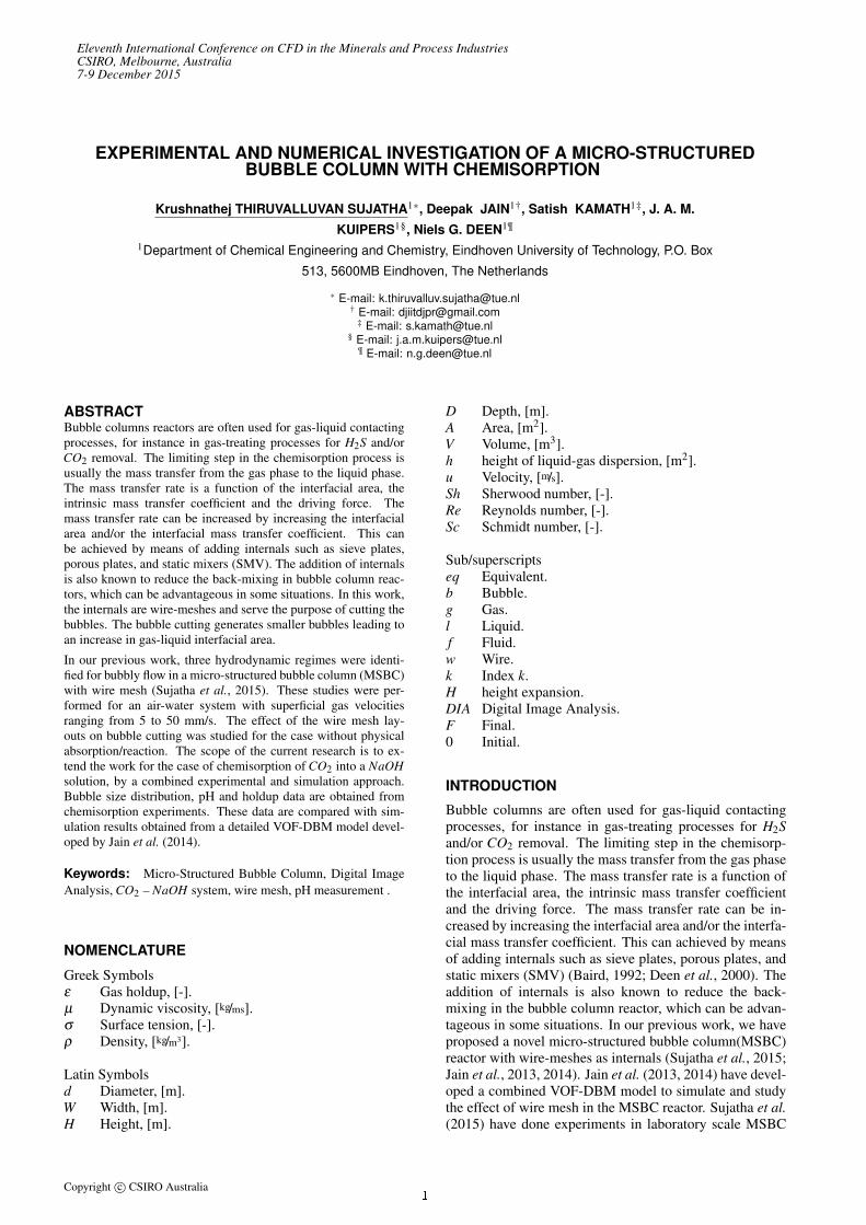
The DIA technique (Lau et al., 2013a,b) was developedto determine the mean diameter deq, bubble size distribu-tions and gas holdup in pseudo-2D bubble column reactor.Sujatha et al. (2015) improved the DIA technique to de-tect very small bubbles. The image analysis algorithm hasfour main operations: a) Image filtering b) separation ofbubbles into solitary and overlapping bubbles c) segmenta-tion of overlapping bubbles using watershedding techniqued) combination of solitary and overlapping bubble images.Image filtering involves operations to obtain a desired im-age involving removal of the inhomogeneous illuminationusing an Otsu filter (Otsu, 1975). The Otsu filter deter-mines the threshold for separating the bubbles from thebackground, by thresholding individual blocks of an im-age. The edges of the bubbles are detected by a Cannyedge detection algorithm. The images are separated intosolitary bubbles and overlapping bubbles using roundnessas a separation criteria. The images with solitary bubblesare segmented by marking the bubbles whereas the overlap-ping bubbles are segmented using the watershed algorithmproposed by Meyer (1994). An example image after bubbledetection is shown in Fig. 1.

A CMOS camera with resolution of 2016 pixel × 2016pixel is used to capture the images of two-phase bubblyflow by using back-lighting to obtain maximum contrastbetween the bubbles and the background. The MSBC is di-vided into three different sections for the purpose of imag-ing and 4000 images are made at 50 Hz for each section .Images from each section have a size of 0.21 m×0.14 mand a small overlap of 0.04 m. The resolution of the imageis 0.11 mm/pixel.The Sauter mean diameter of an image is calculated fromthe equivalent diameter using the following equation:

d32 =

n

∑k=0

d3eq,k

n

∑k=0

d2eq,k

(1)

The probability density function (PDF) for a particular bub-ble diameter class is the ratio of number of bubbles in a par-ticular diameter class(∆deq) to the sum of number of bub-bles in all size classes. Therefore, the PDF of a particular


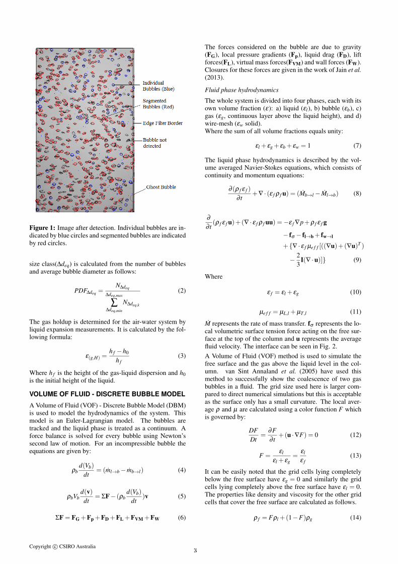
Figure 1: Image after detection. Individual bubbles are in-dicated by blue circles and segmented bubbles are indicatedby red circles.

size class(∆deq) is calculated from the number of bubblesand average bubble diameter as follows:

PDF∆deq =N∆deq

∆deq,max

∑∆deq,min

N∆deq,k

(2)

The gas holdup is determined for the air-water system byliquid expansion measurements. It is calculated by the fol-lowing formula:

ε(g,H) =h f −h0

h f(3)

Where h f is the height of the gas-liquid dispersion and h0is the initial height of the liquid.

VOLUME OF FLUID - DISCRETE BUBBLE MODEL

A Volume of Fluid (VOF) - Discrete Bubble Model (DBM)is used to model the hydrodynamics of the system. Thismodel is an Euler-Lagrangian model. The bubbles aretracked and the liquid phase is treated as a continuum. Aforce balance is solved for every bubble using Newton’ssecond law of motion. For an incompressible bubble theequations are given by:

ρbd(Vb)

dt= (ml→b− mb→l) (4)

ρbVbd(v)dt

= ΣF− (ρbd(Vb)

dt)v (5)

ΣF = FG +Fp +FD +FL +FVM +FW (6)

The forces considered on the bubble are due to gravity(FG), local pressure gradients (Fp), liquid drag (FD), liftforces(FL), virtual mass forces(FVM) and wall forces (FW).Closures for these forces are given in the work of Jain et al.(2013).

Fluid phase hydrodynamics

The whole system is divided into four phases, each with itsown volume fraction (ε): a) liquid (εl), b) bubble (εb), c)gas (εg, continuous layer above the liquid height), and d)wire-mesh (εw solid).Where the sum of all volume fractions equals unity:

εl + εg + εb + εw = 1 (7)

The liquid phase hydrodynamics is described by the vol-ume averaged Navier-Stokes equations, which consists ofcontinuity and momentum equations:

∂ (ρ f ε f )

∂ t+∇ · (ε f ρ f u) = (Mb→l− Ml→b) (8)

∂

∂ t(ρ f ε f u)+(∇ · ε f ρ f uu) =−ε f ∇p+ρ f ε f g

− fσ − fl→b + fw→l

+{∇ · ε f µe f f [((∇u)+(∇u)T )

− 23

I(∇ ·u)]} (9)

Where

ε f = εl + εg (10)

µe f f = µL,l +µT,l (11)

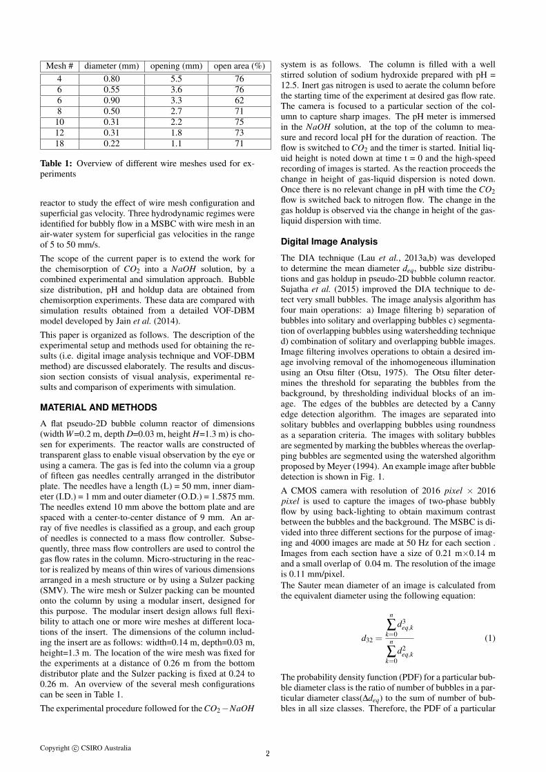
M represents the rate of mass transfer. fσ represents the lo-cal volumetric surface tension force acting on the free sur-face at the top of the column and u represents the averagefluid velocity. The interface can be seen in Fig. 2.A Volume of Fluid (VOF) method is used to simulate thefree surface and the gas above the liquid level in the col-umn. van Sint Annaland et al. (2005) have used thismethod to successfully show the coalescence of two gasbubbles in a fluid. The grid size used here is larger com-pared to direct numerical simulations but this is acceptableas the surface only has a small curvature. The local aver-age ρ and µ are calculated using a color function F whichis governed by:

DFDt

=∂F∂ t

+(u ·∇F) = 0 (12)

F =εl

εl + εg=

εl

ε f(13)

It can be easily noted that the grid cells lying completelybelow the free surface have εg = 0 and similarly the gridcells lying completely above the free surface have εl = 0.The properties like density and viscosity for the other gridcells that cover the free surface are calculated as follows.

ρ f = Fρl +(1−F)ρg (14)


Figure 2: Example snapshot of VOF-DBM simulationshowing bubbles and free surface. Note: the geometry dif-fers from the one used in this work.

ρ f

µ f= F

ρl

µl+(1−F)

ρg

µg(15)

The boundary conditions are applied using a flag matrixconcept. Fig. 3 shows the different values of the flags ofthe pseudo 2-D column. The cells are assigned differentflag values indicating different types of boundary condi-tions that are listed in Table 2.

4 2

3 3

3

1

NX

NZ

Front view Top view

33

3

1

NX

3 NY4

44

4

4

4

4

Figure 3: Boundary conditions for the VOF-DBM; Frontview at j=NY/2 and top view for cells k=2 to k=NZ-1.

The turbulence in the liquid phase due to bubbly flow istaken into account by using a sub-grid scale model pro-posed by Vreman (2004) for the eddy viscosity.Bubble coalescence is accounted for based on the modelproposed by Sommerfeld et al. (2003). The collision timeis determined by the relation reported by Allen and Tildes-ley (1989). Film drainage time for coalescence to occur iscalculated based on the model of Prince and Blanch (1990).When the contact time is less than the film drainage timecoalescence does not occur and the bubbles simply bounce.Otherwise, they coalesce. A detailed description of themodel can be found in Darmana et al. (2005). Bubble

Table 2: Flag meaning for cell boundary conditions

Flag Boundary conditions1 Interior cell, none specified2 Prescribed pressure cell, free slip3 Impermeable wall, no slip, Neumann for species4 Corner cell, none specified

breakup occurs if the inertial force exceeds the surface ten-sion forces, the ratio of which can be represented as Webernumber. The critical Weber number for breakup to occur is12 as determined by Jain et al. (2014). Based on this, a bi-nary breakup model is considered where after break-up thebigger bubble is placed at the position of the parent bub-ble and the smaller bubble is placed randomly around thecentroid of the bigger bubble.

Wire-mesh and cutting

The wire mesh is present in the middle of the column to cutthe bubbles. A simple geometric cutting model proposedby Jain et al. (2013) is incorporated to account for cuttingthe bubbles when they pass the wire mesh. A stochasticfactor called cutting efficiency is introduced into the modelto characterize the fraction of bubbles that is actually cutby the wire mesh. A cutting efficiency 0 means there is nocutting and a value of 1 means all bubbles are eligible toget cut. The drag that the wire-mesh exerts on the liquid istaken into account in Equation 9 (Jain et al., 2013).

Chemical species equations

The species are accounted for through Yj which is the massfraction of species j. Species balances for Ns− 1 compo-nents are solved simultaneously with appropriate boundaryconditions, where Ns is number of components present inthe system. The fraction of the last component can be de-rived from the overall mass balance.

∂

∂ t

(Fε f ρ fYj

)+∇ ·

(Fε f

(ρluYj−Γ j,e f f ∇Yj

))=(

M jb→l− M j

l→b

)+Fε f SR, j (16)

NS

∑j=1

Yj = 1 (17)

SR j is the source term accounting for the production or con-sumption of species j due to chemical reaction.The mass transfer is given by:

m jb = Ek j

l Abρl(Yj∗

l −Y jl ) (18)

Where the mass transfer coefficient kl is calculated througha Sherwood correlation. Several mass transfer correlationsare available in literature for bubbly flows. Brauer (1981)gives a correlation for ellipsoidal bubbles accounting forthe shape of the bubble due to the deformations caused byliquid flow around bubbles:

Sh = 2+0.015×Re0.89B Sc0.7 (19)

The correlation for the enhancement factor (E) provided byWesterterp et al. (1987) is used as proposed by Darmanaet al. (2005).


RESULTS

Visual observation

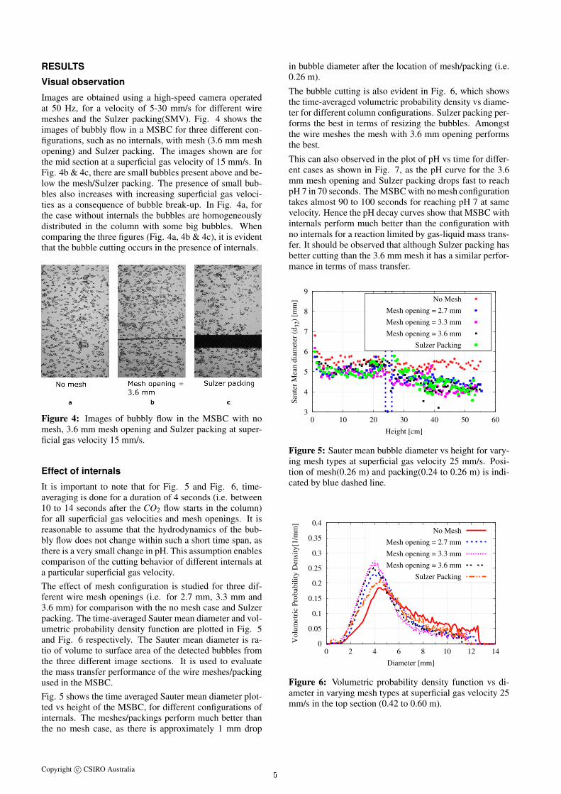
Images are obtained using a high-speed camera operatedat 50 Hz, for a velocity of 5-30 mm/s for different wiremeshes and the Sulzer packing(SMV). Fig. 4 shows theimages of bubbly flow in a MSBC for three different con-figurations, such as no internals, with mesh (3.6 mm meshopening) and Sulzer packing. The images shown are forthe mid section at a superficial gas velocity of 15 mm/s. InFig. 4b & 4c, there are small bubbles present above and be-low the mesh/Sulzer packing. The presence of small bub-bles also increases with increasing superficial gas veloci-ties as a consequence of bubble break-up. In Fig. 4a, forthe case without internals the bubbles are homogeneouslydistributed in the column with some big bubbles. Whencomparing the three figures (Fig. 4a, 4b & 4c), it is evidentthat the bubble cutting occurs in the presence of internals.

Figure 4: Images of bubbly flow in the MSBC with nomesh, 3.6 mm mesh opening and Sulzer packing at super-ficial gas velocity 15 mm/s.

Effect of internals

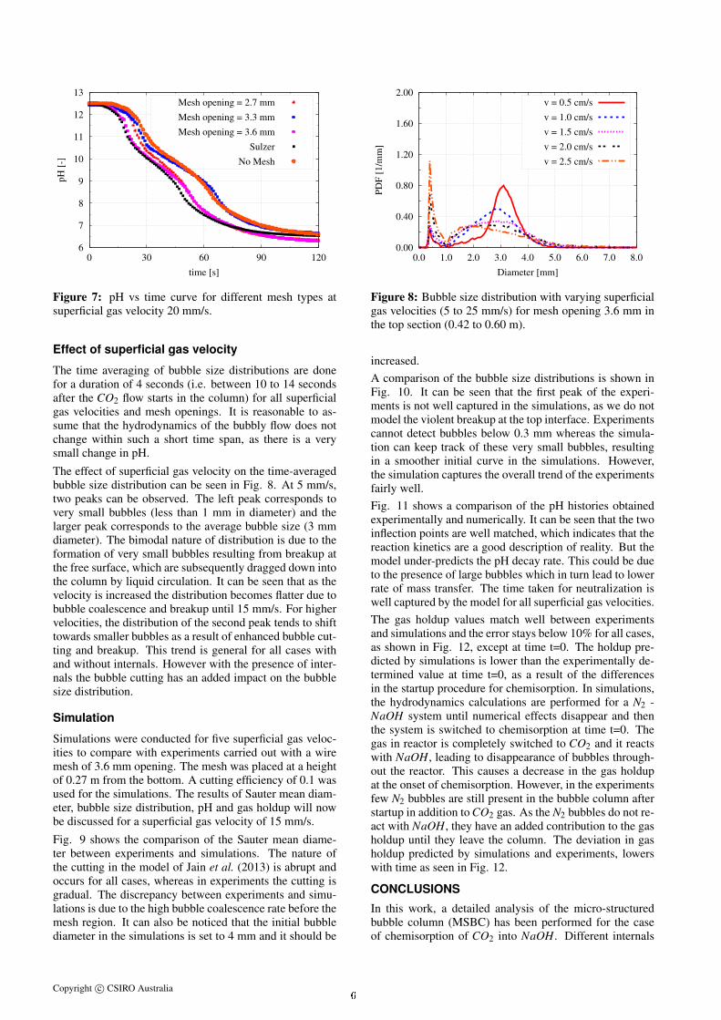
It is important to note that for Fig. 5 and Fig. 6, time-averaging is done for a duration of 4 seconds (i.e. between10 to 14 seconds after the CO2 flow starts in the column)for all superficial gas velocities and mesh openings. It isreasonable to assume that the hydrodynamics of the bub-bly flow does not change within such a short time span, asthere is a very small change in pH. This assumption enablescomparison of the cutting behavior of different internals ata particular superficial gas velocity.The effect of mesh configuration is studied for three dif-ferent wire mesh openings (i.e. for 2.7 mm, 3.3 mm and3.6 mm) for comparison with the no mesh case and Sulzerpacking. The time-averaged Sauter mean diameter and vol-umetric probability density function are plotted in Fig. 5and Fig. 6 respectively. The Sauter mean diameter is ra-tio of volume to surface area of the detected bubbles fromthe three different image sections. It is used to evaluatethe mass transfer performance of the wire meshes/packingused in the MSBC.Fig. 5 shows the time averaged Sauter mean diameter plot-ted vs height of the MSBC, for different configurations ofinternals. The meshes/packings perform much better thanthe no mesh case, as there is approximately 1 mm drop

in bubble diameter after the location of mesh/packing (i.e.0.26 m).

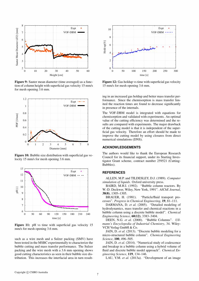
The bubble cutting is also evident in Fig. 6, which showsthe time-averaged volumetric probability density vs diame-ter for different column configurations. Sulzer packing per-forms the best in terms of resizing the bubbles. Amongstthe wire meshes the mesh with 3.6 mm opening performsthe best.

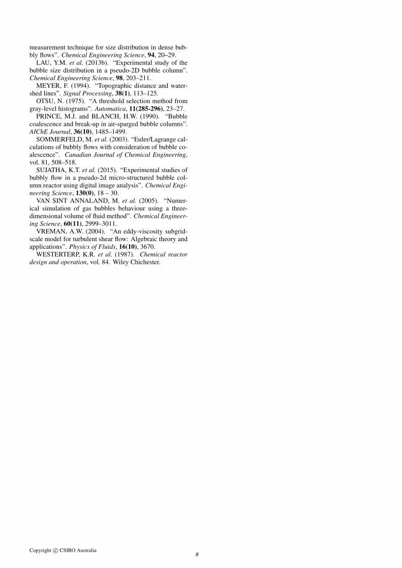
This can also observed in the plot of pH vs time for differ-ent cases as shown in Fig. 7, as the pH curve for the 3.6mm mesh opening and Sulzer packing drops fast to reachpH 7 in 70 seconds. The MSBC with no mesh configurationtakes almost 90 to 100 seconds for reaching pH 7 at samevelocity. Hence the pH decay curves show that MSBC withinternals perform much better than the configuration withno internals for a reaction limited by gas-liquid mass trans-fer. It should be observed that although Sulzer packing hasbetter cutting than the 3.6 mm mesh it has a similar perfor-mance in terms of mass transfer.

3

4

5

6

7

8

9

0 10 20 30 40 50 60

Sau

ter

Mea

n d

iam

eter

(d

32)

[mm

]

Height [cm]

No Mesh

Mesh opening = 2.7 mm



Sulzer Packing

Figure 5: Sauter mean bubble diameter vs height for vary-ing mesh types at superficial gas velocity 25 mm/s. Posi-tion of mesh(0.26 m) and packing(0.24 to 0.26 m) is indi-cated by blue dashed line.

0

0.05

0.1

0.15

0.2

0.25

0.3

0.35

0.4

0 2 4 6 8 10 12 14

Vo

lum

etri

c P

rob

abil

ity

Den

sity

[1/m

m]

Diameter [mm]

No Mesh




Sulzer Packing

Figure 6: Volumetric probability density function vs di-ameter in varying mesh types at superficial gas velocity 25mm/s in the top section (0.42 to 0.60 m).


6

7

8

9

10

11

12

13

0 30 60 90 120

pH

[-]

time [s]




Sulzer

No Mesh

Figure 7: pH vs time curve for different mesh types atsuperficial gas velocity 20 mm/s.

Effect of superficial gas velocity

The time averaging of bubble size distributions are donefor a duration of 4 seconds (i.e. between 10 to 14 secondsafter the CO2 flow starts in the column) for all superficialgas velocities and mesh openings. It is reasonable to as-sume that the hydrodynamics of the bubbly flow does notchange within such a short time span, as there is a verysmall change in pH.

The effect of superficial gas velocity on the time-averagedbubble size distribution can be seen in Fig. 8. At 5 mm/s,two peaks can be observed. The left peak corresponds tovery small bubbles (less than 1 mm in diameter) and thelarger peak corresponds to the average bubble size (3 mmdiameter). The bimodal nature of distribution is due to theformation of very small bubbles resulting from breakup atthe free surface, which are subsequently dragged down intothe column by liquid circulation. It can be seen that as thevelocity is increased the distribution becomes flatter due tobubble coalescence and breakup until 15 mm/s. For highervelocities, the distribution of the second peak tends to shifttowards smaller bubbles as a result of enhanced bubble cut-ting and breakup. This trend is general for all cases withand without internals. However with the presence of inter-nals the bubble cutting has an added impact on the bubblesize distribution.

Simulation

Simulations were conducted for five superficial gas veloc-ities to compare with experiments carried out with a wiremesh of 3.6 mm opening. The mesh was placed at a heightof 0.27 m from the bottom. A cutting efficiency of 0.1 wasused for the simulations. The results of Sauter mean diam-eter, bubble size distribution, pH and gas holdup will nowbe discussed for a superficial gas velocity of 15 mm/s.

Fig. 9 shows the comparison of the Sauter mean diame-ter between experiments and simulations. The nature ofthe cutting in the model of Jain et al. (2013) is abrupt andoccurs for all cases, whereas in experiments the cutting isgradual. The discrepancy between experiments and simu-lations is due to the high bubble coalescence rate before themesh region. It can also be noticed that the initial bubblediameter in the simulations is set to 4 mm and it should be

0.00

0.40

0.80

1.20

1.60

2.00

0.0 1.0 2.0 3.0 4.0 5.0 6.0 7.0 8.0

PD

F [

1/m

m]

Diameter [mm]

v = 0.5 cm/s

v = 1.0 cm/s

v = 1.5 cm/s

v = 2.0 cm/s

v = 2.5 cm/s

Figure 8: Bubble size distribution with varying superficialgas velocities (5 to 25 mm/s) for mesh opening 3.6 mm inthe top section (0.42 to 0.60 m).

increased.A comparison of the bubble size distributions is shown inFig. 10. It can be seen that the first peak of the experi-ments is not well captured in the simulations, as we do notmodel the violent breakup at the top interface. Experimentscannot detect bubbles below 0.3 mm whereas the simula-tion can keep track of these very small bubbles, resultingin a smoother initial curve in the simulations. However,the simulation captures the overall trend of the experimentsfairly well.Fig. 11 shows a comparison of the pH histories obtainedexperimentally and numerically. It can be seen that the twoinflection points are well matched, which indicates that thereaction kinetics are a good description of reality. But themodel under-predicts the pH decay rate. This could be dueto the presence of large bubbles which in turn lead to lowerrate of mass transfer. The time taken for neutralization iswell captured by the model for all superficial gas velocities.The gas holdup values match well between experimentsand simulations and the error stays below 10% for all cases,as shown in Fig. 12, except at time t=0. The holdup pre-dicted by simulations is lower than the experimentally de-termined value at time t=0, as a result of the differencesin the startup procedure for chemisorption. In simulations,the hydrodynamics calculations are performed for a N2 -NaOH system until numerical effects disappear and thenthe system is switched to chemisorption at time t=0. Thegas in reactor is completely switched to CO2 and it reactswith NaOH, leading to disappearance of bubbles through-out the reactor. This causes a decrease in the gas holdupat the onset of chemisorption. However, in the experimentsfew N2 bubbles are still present in the bubble column afterstartup in addition to CO2 gas. As the N2 bubbles do not re-act with NaOH, they have an added contribution to the gasholdup until they leave the column. The deviation in gasholdup predicted by simulations and experiments, lowerswith time as seen in Fig. 12.

CONCLUSIONS

In this work, a detailed analysis of the micro-structuredbubble column (MSBC) has been performed for the caseof chemisorption of CO2 into NaOH. Different internals


2

3

4

5

6

7

8

0 10 20 30 40 50 60

Sau

ter

Mea

n D

iam

eter

(d

32

) [m

m]

Height [cm]

Expt

VOF-DBM

Figure 9: Sauter mean diameter (time averaged) as a func-tion of column height with superficial gas velocity 15 mm/sfor mesh opening 3.6 mm.

0

0.2

0.4

0.6

0.8

1

1.2

0 1 2 3 4 5 6 7 8

PD

F [

1/m

m]

Diameter [mm]

Expt

VOF-DBM

Figure 10: Bubble size distribution with superficial gas ve-locity 15 mm/s for mesh opening 3.6 mm.

6

7

8

9

10

11

12

13

0 30 60 90 120 150 180 210 240

pH

[-]

time [s]

Expt

VOF-DBM

Figure 11: pH vs time with superficial gas velocity 15mm/s for mesh opening 3.6 mm.

such as a wire mesh and a Sulzer packing (SMV) havebeen tested in the MSBC experimentally to characterize thebubble cutting and mass transfer performance. The Sulzerpacking and the wire mesh with a 3.6 mm opening showsgood cutting characteristics as seen in their bubble size dis-tribution. This increases the interfacial area in turn result-

0

2

4

6

8

10

0 50 100 150 200 250 300

Ho

ld-u

p[%

]

time [s]

Expt

VOF-DBM

Figure 12: Gas holdup vs time with superficial gas velocity15 mm/s for mesh opening 3.6 mm.

ing in an increased gas holdup and better mass transfer per-formance. Since the chemisorption is mass transfer lim-ited the reaction times are found to decrease significantlyin presence of the internals.

The VOF-DBM model is integrated with equations forchemisorption and validated with experiments. An optimalvalue of the cutting efficiency was determined and the re-sults are compared with experiments. The major drawbackof the cutting model is that it is independent of the super-ficial gas velocity. Therefore an effort should be made toimprove the cutting model by using closures from directnumerical simulations (DNS).

ACKNOWLEDGEMENTS

The authors would like to thank the European ResearchCouncil for its financial support, under its Starting Inves-tigator Grant scheme, contract number 259521 (Cutting-Bubbles).

REFERENCES

ALLEN, M.P. and TILDESLEY, D.J. (1989). Computersimulation of liquids. Oxford university press.

BAIRD, M.H.I. (1992). “Bubble column reactors. ByW.-D. Deckwer, Wiley, New York, 1991”. AIChE Journal,38(8), 1305–1305.

BRAUER, H. (1981). “Particle/fluid transport pro-cesses”. Progress in Chemical Engineering, 19, 81–111.

DARMANA, D. et al. (2005). “Detailed modeling ofhydrodynamics, mass transfer and chemical reactions in abubble column using a discrete bubble model”. ChemicalEngineering Science, 60(12), 3383–3404.

DEEN, N.G. et al. (2000). “Bubble Columns”. Ull-mann’s Encyclopedia of Industrial Chemistry, 34. Wiley-VCH Verlag GmbH & Co.

JAIN, D. et al. (2013). “Discrete bubble modeling for amicro-structured bubble column”. Chemical EngineeringScience, 100, 496–505.

JAIN, D. et al. (2014). “Numerical study of coalescenceand breakup in a bubble column using a hybrid volume offluid and discrete bubble model approach”. Chemical En-gineering Science, 119, 134–146.

LAU, Y.M. et al. (2013a). “Development of an image


measurement technique for size distribution in dense bub-bly flows”. Chemical Engineering Science, 94, 20–29.

LAU, Y.M. et al. (2013b). “Experimental study of thebubble size distribution in a pseudo-2D bubble column”.Chemical Engineering Science, 98, 203–211.

MEYER, F. (1994). “Topographic distance and water-shed lines”. Signal Processing, 38(1), 113–125.

OTSU, N. (1975). “A threshold selection method fromgray-level histograms”. Automatica, 11(285-296), 23–27.

PRINCE, M.J. and BLANCH, H.W. (1990). “Bubblecoalescence and break-up in air-sparged bubble columns”.AIChE Journal, 36(10), 1485–1499.

SOMMERFELD, M. et al. (2003). “Euler/Lagrange cal-culations of bubbly flows with consideration of bubble co-alescence”. Canadian Journal of Chemical Engineering,vol. 81, 508–518.

SUJATHA, K.T. et al. (2015). “Experimental studies ofbubbly flow in a pseudo-2d micro-structured bubble col-umn reactor using digital image analysis”. Chemical Engi-neering Science, 130(0), 18 – 30.

VAN SINT ANNALAND, M. et al. (2005). “Numer-ical simulation of gas bubbles behaviour using a three-dimensional volume of fluid method”. Chemical Engineer-ing Science, 60(11), 2999–3011.

VREMAN, A.W. (2004). “An eddy-viscosity subgrid-scale model for turbulent shear flow: Algebraic theory andapplications”. Physics of Fluids, 16(10), 3670.

WESTERTERP, K.R. et al. (1987). Chemical reactordesign and operation, vol. 84. Wiley Chichester.


Documents

EXPERIMENTAL AND NUMERICAL INVESTIGATION OF … · EXPERIMENTAL AND NUMERICAL INVESTIGATION OF A MICRO ... The bubble cutting generates smaller bubbles ... sure and record local pH