1

Experimental and Computational Flow Field Studies of a MAV-scale

Cycloidal Rotor in Forward Flight

Tejaswi Jarugumilli1 Andrew H. Lind

2 Moble Benedict

3

Alfred Gessow Rotorcraft Center,

University of Maryland, College Park, MD

Vinod K. Lakshminarayan4

Dept. of Aeronautics and Astronautics

Stanford University, CA Anya R. Jones

5 Inderjit Chopra

6

Alfred Gessow Rotorcraft Center, University of Maryland, College Park, MD

ABSTRACT

This paper provides a fundamental examination of the flow physics for a two-bladed MAV-scale cycloidal rotor (or

cyclorotor) in forward flight using experimental particle image velocimetry (PIV) measurements, computational studies (2D

CFD) and time-averaged performance measurements. A simple aerodynamic analysis using time-averaged flow field

measurements from PIV is used to develop a basic understanding of the distribution of blade aerodynamic forces and power

along the rotor azimuth. The incoming flow velocity is shown to decrease in magnitude as the flow passes through the upper

half of the rotor. This is attributed to power extraction by the blades in the upper-frontal region of the rotor azimuth. Flow field

measurements also show a significant increase in flow velocity across the lower half of the rotor cage. The aerodynamic

analysis demonstrates that the blades accelerate the flow through the lower-aft region of the rotor, where they operate in a high

dynamic pressure environment with a large positive effective angle of attack. CFD-predicted values of instantaneous

aerodynamic forces reveal that the aft section of the rotor is the primary region of force production. Phase-averaged flow field

measurements are also analyzed. These results reveal two blade wakes in the flow, formed by each of the two blades. Analysis

of the blades at several azimuthal positions revealed two significant blade-wake interactions in the aft of the cyclorotor. The

locations of these blade-wake interactions are correlated with force peaks in the CFD-predicted instantaneous blade forces,

implying that unsteady aerodynamic interactions play an important role in the lift and propulsive force generation of the

cyclorotor.

NOTATION

b Blade span

c Blade chord length

D Rotor diameter

Nb Number of blades

U∞ Freestreem velocity

X, Y, Z Rotor coordinate system

u Horizontal component of velocity

v Vertical component of velocity

α Angle of attack

αi Virtual incidence angle

_______________________________ Presented at the 69

th Annual Forum, Phoenix, Arizona, May 21-23,

2013. Copyright © 2013 by the authors. Published by the AHS

International with permission. All Rights reserved. 1 Graduate Research Assistant. jtsn423@umd.edu

2 Graduate Research Assistant. alind@umd.edu

3 Assistant Research Scientist. moble@umd.edu

4 Postdoctoral Fellow. vinodkl@stanford.edu

5 Assistant Professor. arjones@umd.edu

6 Alfred Gessow Professor and Director. chopra@umd.edu

INTRODUCTION

In response to the increasing need for smaller unmanned

aerial vehicles (UAVs) and rapid advancements in

miniaturized electronic systems during the past decade, a

new class of flying machines called micro air vehicles

(MAVs) has emerged. The ultimate design goals for MAVs

include a gross takeoff weight of less than 100 g and

maximum length dimensions less than 15 cm (Ref. 1). The

potential for MAVs to perform a wide range of missions in

cost-effective and low-risk ways could make them powerful

assets in both military and civilian applications in the future.

θ Pitch angle

θA Half peak-to-peak pitch amplitude

μ Advance ratio

Φ Rotor phase angle

Ω Rotor rpm

Ѱ Blade azimuthal position

2

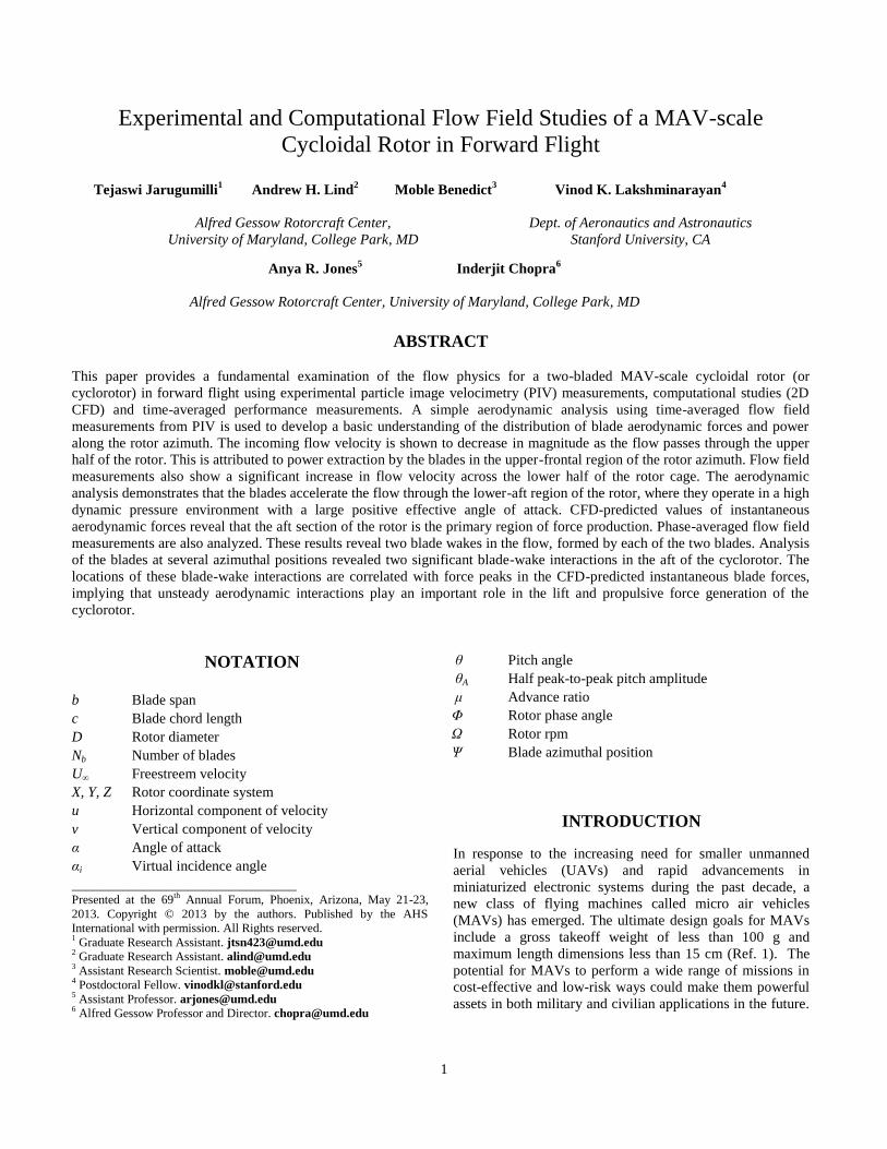
(a) Cycloidal rotor. (b) Cycloidal-rotor based MAV capable of autonomous

hover developed at the University of Maryland.

Figure 1. Cycloidal rotor system.

Some examples of potential missions include surveillance

and reconnaissance in the battlefield, biochemical sensing,

traffic monitoring, fire and rescue operations, border

surveillance, wildlife surveys, power line inspection and

real estate aerial photography.

Currently, the prevailing choice for a hover-capable MAV

utilizes a conventional edge-wise rotor. However, MAVs

operate in a low Reynolds number flight regime where a

conventional rotor faces severely degraded aerodynamic

performance (Ref. 2). Recently, a cycloidal-rotor

(cyclorotor) based MAV has been proposed as a potential

alternative (Fig. 1) (Ref. 3). The cyclorotor consists of a set

of blades that follow a circular trajectory about a horizontal

axis of rotation (Fig. 1(a)). A passive four-bar pitching

mechanism allows each blade to achieve positive pitch

angles in both halves of its circular trajectory (Fig. 2).

These pitching kinematics allow the rotor to produce a net

non-zero aerodynamic force. The magnitude and direction

of the net force vector can be controlled by varying the

amplitude and phasing of the blade pitching kinematics.

The advantages of a cycloidal rotor system stem from its

potential for higher aerodynamic efficiency, increased

maneuverability and high-speed forward flight. Unlike a

conventional helicopter rotor, where aerodynamic

conditions vary significantly along the blade span, all span-

wise blade elements of the cyclorotor operate under similar

conditions (i.e. similar flow velocities, Reynolds numbers,

and angles of incidence). The relatively uniform

distribution of forces along the blade span allows the

cyclorotor to be more easily optimized for maximum

aerodynamic efficiency. Previous experimental studies have

shown that a cyclorotor can achieve a higher aerodynamic

power loading (thrust/power) in hover compared to a

conventional rotor of similar scale (Ref. 3). A second

advantage of a cyclorotor is its thrust vectoring capability.

The net thrust vector can be instantaneously set to any

direction perpendicular to the axis of rotation by

introducing a phasing in the pitching kinematics. Thus, the

cyclorotor concept may provide relatively better

maneuverability compared to a conventional rotor based

MAV, making it ideal for operations in highly confined and

gusty environments. Furthermore, previous studies have

shown several advantages of the cyclorotor in forward

flight (Refs. 4-5), two of which include the achievement of

high forward flight speeds (up to 13 m/s) with significant

reductions in power consumption and the ability to

transition from hover to forward flight without significant

changes to vehicle attitude or configuration.

The cycloidal rotor concept has been explored for aviation

applications since the early 20th

century (Refs. 6-9).

However, experimental data and analytical models for rotor

performance are scarce, especially at MAV-scales. Most

previous experiments were conducted at relatively large

scales (Re>100,000) and primarily restricted to the hover

condition (Refs. 6-12). A detailed background on many of

these earlier studies is presented in Ref. 13.

The present work is a continuation of previous efforts at the

University of Maryland aimed to understand the forward

flight performance of a MAV-scale cyclorotor (Refs. 4-5).

Previous studies primarily involved time-averaged

experimental performance measurements of the rotor lift,

propulsive force and power at different advance ratios and

varying blade pitching kinematics (i.e. blade pitch

amplitude, pitch phase angle and symmetry of pitching).

3

The current work utilizes time-resolved, planar particle

image velocimetry (PIV) techniques to gain a fundamental

understanding of the flow environment. This is the first

known study which employs experimental techniques to

examine the flow field of a cyclorotor in forward flight. In

addition to the PIV studies, computational studies (2D

CFD) and time-averaged experimental performance

measurements were conducted. The key contributions of the

CFD studies in this work are predictions of the

instantaneous blade forces and power along the rotor

azimuth. In general, it is difficult to implement devices (e.g.

pressure taps, strain gages) to experimentally measure

instantaneous blade forces on MAV-scale rotary wing

systems due to the imposed space constraints and high

centrifugal load environments in which they operate.

Therefore, the CFD studies are integral to this work as they

provide instantaneous aerodynamic blade loads.

The goal of the current work is to develop a fundamental

understanding of the governing flow physics and how it

affects the force production on a cyclorotor in forward

flight. In turn, the findings in this study may aid in the

design and development of an efficient, high-speed flight

capable cyclocopter MAV.

The remaining sections of the paper are organized as

follows. First, the definitions and rotor coordinate system

for the cyclorotor are introduced. Next, the experimental

setup and procedures for the PIV studies and performance

measurements are discussed, followed by the methodology

and validation for the 2D CFD studies. Flow field results

are presented and correlated with experimental and

computational aerodynamic forces. Lastly, the key

conclusions from this study are summarized.

DEFINITIONS AND ROTOR COORDINATE

SYSTEM

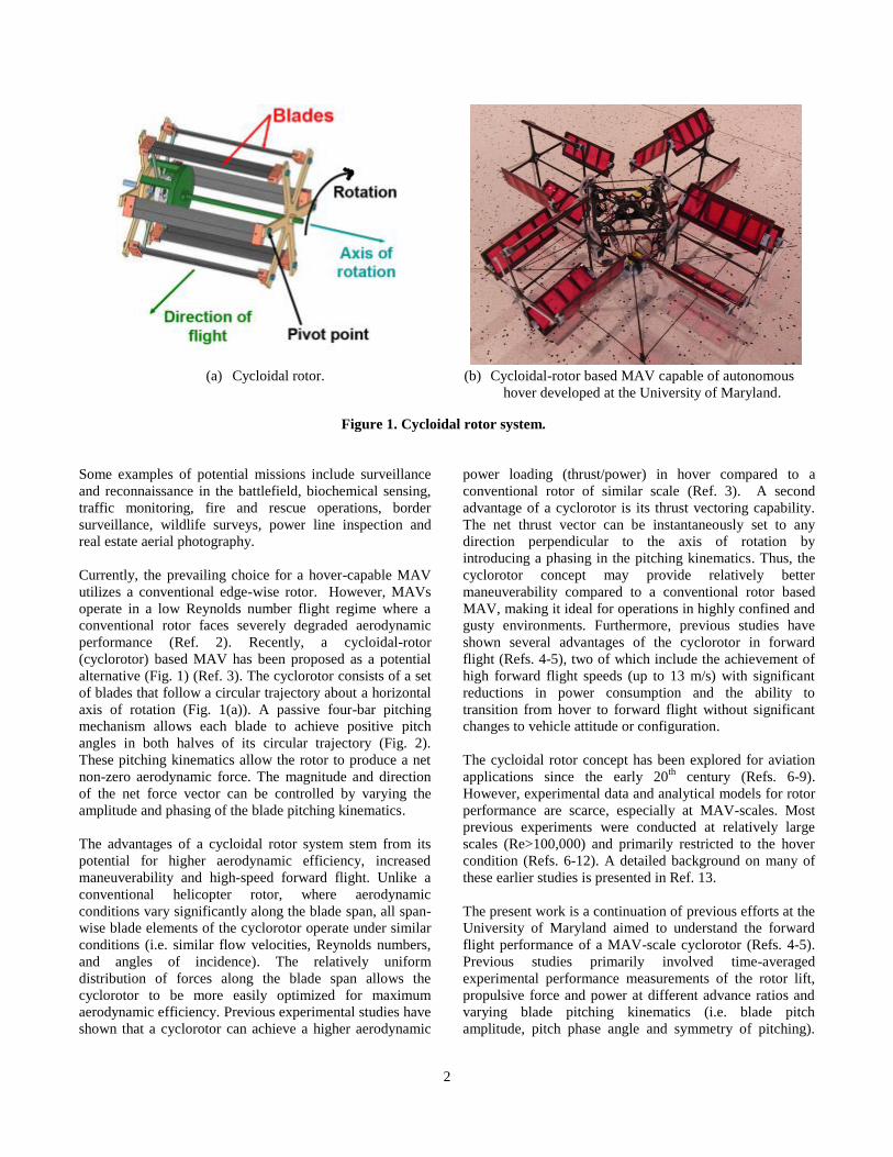
The coordinate system for the cyclorotor used in the present

study is shown in Fig. 2. The rotor operates in the

clockwise direction, with the freestream velocity flowing

from left to right. The azimuthal position of each blade, Ѱ,

is measured in the clockwise direction originating from the

positive Y-axis. The blade pitch angle, θ, is the angle

formed by the blade chord line and the tangent to the

circular trajectory of the blade. The blade pitching

kinematics are represented as a sinusoidal function:

( ) ( )

Here, θA is half the total peak-to-peak pitch amplitude and

Φ is the pitch phase angle. For all the cases considered in

this work, the phase angle is maintained at Φ=90°. This

corresponds to the blades achieving maximum pitch angles

at azimuthal locations of Ѱ=0° (rotor front) and Ѱ=180°

(rotor rear/aft). This is illustrated in Fig. 2. In addition, the

peak-to-peak pitch amplitude is maintained constant at 70°

(i.e. =35°) for all cases.

Figure 2. Rotor coordinate system (forward flight).

This study examined rotor performance at different advance

ratios (μ), the ratio of freestream flow velocity to the blade

tip speed:

μ =

The rotor lift force is defined as the net aerodynamic force

produced in the +Z-direction (perpendicular to the

freestream) and the propulsive thrust is the net aerodynamic

force in the +Y-direction (Fig. 2). The total aerodynamic

power includes the induced power, profile power and

rotational flow losses associated with the blades. The power

associated with the rotation of the blade support structure

(e.g. endplates, linkages, etc.) was removed from the power

measurements to isolate the aerodynamic power of the

blades.

EXPERIMENTAL SETUP AND

PROCEDURES

In the current work, flow field measurements were obtained

using time-resolved, planar (two-component) particle image

velocimetry (PIV). Time-averaged performance

measurements were acquired using a custom-built force

balance system. The experimental work is compared with a

computational fluid dynamics (CFD) analysis. The current

section describes each setup in detail as well as the

validation techniques for the CFD analysis.

U∞

(Aft) (Front)

(Bottom)

(Top)

4

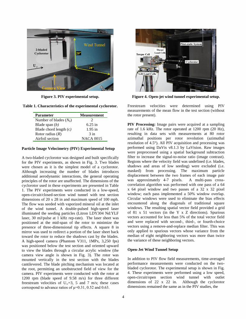
Figure 3. PIV experimental setup.

Table 1. Characteristics of the experimental cyclorotor.

Parameter Measurement

Number of blades (Nb) 2

Blade span (b) 6.25 in

Blade chord length (c) 1.95 in

Rotor radius (R) 3 in

Airfoil section NACA 0015

Particle Image Velocimetry (PIV) Experimental Setup

A two-bladed cyclorotor was designed and built specifically

for the PIV experiments, as shown in Fig. 3. Two blades

were chosen as it is the simplest model of a cyclorotor.

Although increasing the number of blades introduces

additional aerodynamic interactions, the general operating

principles of the rotor are unaffected. The dimensions of the

cyclorotor used in these experiments are presented in Table

1. The PIV experiments were conducted in a low-speed,

open-circuit/closed-section wind tunnel with test section

dimensions of 20 x 28 in and maximum speed of 100 mph.

The flow was seeded with vaporized mineral oil at the inlet

of the wind tunnel. A double-pulsed high-speed laser

illuminated the seeding particles (Litron LDY304 Nd:YLF

laser, 30 mJ/pulse at 1 kHz rep-rate). The laser sheet was

positioned at the mid-span of the rotor to minimize the

presence of three-dimensional tip effects. A square 8 in

mirror was used to redirect a portion of the laser sheet back

toward the rotor to reduce the shadows cast by the blades.

A high-speed camera (Phantom V311, 1MPx, 3,250 fps)

was positioned below the test section and oriented upward

to view the blades through a circular acrylic window (the

camera view angle is shown in Fig. 3). The rotor was

mounted vertically in the test section with the blades

cantilevered. The blade pitching mechanism was located at

the root, permitting an unobstructed field of view for the

camera. PIV experiments were conducted with the rotor at

1200 rpm (blade speed of 9.58 m/s) for three different

freestream velocities of U∞=3, 5 and 7 m/s; these cases

correspond to advance ratios of μ=0.31, 0.52 and 0.63.

Figure 4. Open-jet wind tunnel experimental setup.

Freestream velocities were determined using PIV

measurements of the mean flow in the test section (without

the rotor present).

PIV Processing: Image pairs were acquired at a sampling

rate of 1.6 kHz. The rotor operated at 1200 rpm (20 Hz),

resulting in data sets with measurements at 80 rotor

azimuthal positions per rotor revolution (azimuthal

resolution of 4.5°). All PIV acquisition and processing was

performed using DaVis v8.1.3 by LaVision. Raw images

were preprocessed using a spatial background subtraction

filter to increase the signal-to-noise ratio (image contrast).

Regions where the velocity field was undefined (i.e. blades,

shadows and areas of low seeding) were excluded (i.e.

masked) from processing. The maximum particle

displacement between the two frames of each image pair

was approximately 4-7 pixels. A multi-pass cross-

correlation algorithm was performed with one pass of a 64

x 64 pixel window and two passes of a 32 x 32 pixel

window; each pass implemented a 50% window overlap.

Circular windows were used to eliminate the bias effects

encountered along the diagonals of traditional square

windows. The resulting spatial vector field provided a grid

of 81 x 51 vectors (in the Y x Z directions). Spurious

vectors accounted for less than 5% of the total vector field

and were replaced with second-, third-, or fourth-choice

vectors using a remove-and-replace median filter. This was

only applied to spurious vectors whose variance from the

median of eight neighboring vectors was more than twice

the variance of these neighboring vectors.

Open-Jet Wind Tunnel Setup

In addition to PIV flow field measurements, time-averaged

performance measurements were conducted on the two-

bladed cyclorotor. The experimental setup is shown in Fig.

4. These experiments were performed using a low speed,

open-circuit/open section wind tunnel with outlet

dimensions of 22 x 22 in. Although the cyclorotor

dimensions remained the same as in the PIV studies, the

Camera View

5

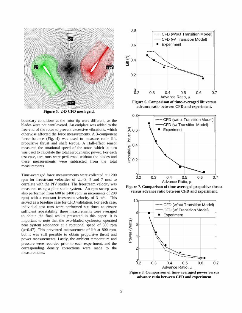
Figure 5. 2-D CFD mesh grid.

boundary conditions at the rotor tip were different, as the

blades were not cantilevered. An endplate was added to the

free-end of the rotor to prevent excessive vibrations, which

otherwise affected the force measurements. A 3-component

force balance (Fig. 4) was used to measure rotor lift,

propulsive thrust and shaft torque. A Hall-effect sensor

measured the rotational speed of the rotor, which in turn

was used to calculate the total aerodynamic power. For each

test case, tare runs were performed without the blades and

these measurements were subtracted from the total

measurements.

Time-averaged force measurements were collected at 1200

rpm for freestream velocities of U∞=3, 5 and 7 m/s, to

correlate with the PIV studies. The freestream velocity was

measured using a pitot-static system. An rpm sweep was

also performed from 600 to 1400 rpm (in increments of 200

rpm) with a constant freestream velocity of 3 m/s. This

served as a baseline case for CFD validation. For each case,

individual test runs were performed six times to ensure

sufficient repeatability; these measurements were averaged

to obtain the final results presented in this paper. It is

important to note that the two-bladed cyclorotor operated

near system resonance at a rotational speed of 800 rpm

(μ=0.47). This prevented measurement of lift at 800 rpm,

but it was still possible to obtain propulsive thrust and

power measurements. Lastly, the ambient temperature and

pressure were recorded prior to each experiment, and the

corresponding density corrections were made to the

measurements.

Figure 6. Comparison of time-averaged lift versus

advance ratio between CFD and experiment.

Figure 7. Comparison of time-averaged propulsive thrust

versus advance ratio between CFD and experiment.

Figure 8. Comparison of time-averaged power versus

advance ratio between CFD and experiment

0.2 0.3 0.4 0.5 0.6 0.70

0.2

0.4

0.6

0.8

Advance Ratio,

Lift (N

)

CFD (w/out Transition Model)

CFD (w/ Transition Model)

Experiment

0.2 0.3 0.4 0.5 0.6 0.70

0.2

0.4

0.6

0.8

Advance Ratio,

Pro

puls

ive T

hru

st (N

)

CFD (w/out Transition Model)

CFD (w/ Transition Model)

Experiment

0.2 0.3 0.4 0.5 0.6 0.70

2

4

6

8

10

Advance Ratio,

Pow

er

(Watts)

CFD (w/out Transition Model)

CFD (w/ Transition Model)

Experiment

6

CFD METHODOLOGY AND VALIDATION

A 2-D CFD study was also conducted to understand the

flow physics of the cyclorotor. The details of the flow

solver and grid system used are discussed below.

Flow Solver: 2-D simulations of the cycloidal rotor were

undertaken using a compressible structured overset RANS

solver, OVERTURNS (Ref. 14). This overset structured

mesh solver uses the diagonal form of the implicit

approximate factorization method developed by Pulliam

and Chaussee (Ref. 15) with a preconditioned dual-time

scheme to solve the compressible RANS equations.

Computations are performed in the inertial frame in a time-

accurate manner. A third-order MUSCL scheme (Ref. 16)

with Roe flux difference splitting (Ref. 17) and Koren’s

limiter (Ref. 18) is used to compute the inviscid terms, and

second-order central differencing is used for the viscous

terms. Due to the relatively low operating Mach numbers of

the present cyclorotor, the inclusion of a low Mach pre-

conditioner based on Turkel’s (Ref. 19) method accelerates

the convergence and ensures accuracy of the solution.

Spalart-Allmaras (SA) (Ref. 20) turbulence model is

employed for RANS closure. This one-equation model has

the advantages of ease of implementation, computational

efficiency and numerical stability. Furthermore, because of

the transitional nature of the flow-field, the CFD

simulations were performed with and without the use of a

transition model. A two equation - SA model of

Medida and Baeder (Ref. 22) is employed in the

simulations using the transition model.

Grid System: An overset system of meshes, consisting of

C-type airfoil mesh for each blade and a cylindrical

background mesh is used for the computation. The airfoil

meshes have 255 x 55 grid points in the wraparound and

normal directions, respectively. The background cylindrical

mesh has 245 x 221 points in the azimuthal and radial

directions, respectively. An implicit hole-cutting method

developed by Lee (Ref. 21) and refined by Lakshminarayan

(Ref. 14) is used to find the connectivity information

between the overset meshes. Figure 5 shows the mesh

system. In this figure, only the field points (points where

the flow equations are solved) are shown. All the points

that are blanked out either receive no information from

another mesh or lie inside a solid body and therefore do not

have a valid solution.

CFD vs. Experiment: Time-Averaged Force Comparison

Prior to utilizing the instantaneous force data predicted by

CFD, the time-averaged lift, propulsive thrust and power

were validated with the experimental measurements.

Figures 6-8 show a comparison between the CFD

predictions and experimentally measured values for time-

averaged aerodynamic forces and power. The CFD-

predicted values show strong correlation with the

experimental measurements, both with and without the

transition model. However, the CFD results with the

transition model show better correlation with experiment;

therefore, all CFD results presented in the following

sections include the transition model. Even though the use

of a transition model improves the prediction, the results

without a transition model also showed a good qualitative

agreement and such simulations might still be valuable if a

CFD code is not equipped with a transition model.

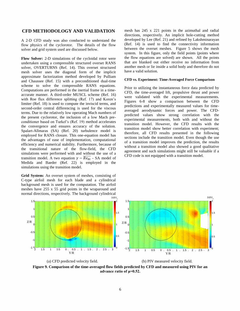
(a) CFD predicted velocity field. (b) PIV measured velocity field.

Figure 9. Comparison of the time-averaged flow fields predicted by CFD and measured using PIV for an

advance ratio of μ=0.52.

y/R

z/R

-2 -1.5 -1 -0.5 0 0.5 1 1.5 2 2.5 3-1.5

-1

-0.5

0

0.5

1

1.5

|U|/U

0

0.5

1

1.5

2

y/R

z/R

-2 -1.5 -1 -0.5 0 0.5 1 1.5 2 2.5 3-1.5

-1

-0.5

0

0.5

1

1.5

|U|/U

0

0.5

1

1.5

2

Y/R Y/R

Z/R Z/R

- - - - - - - - - - - -

7

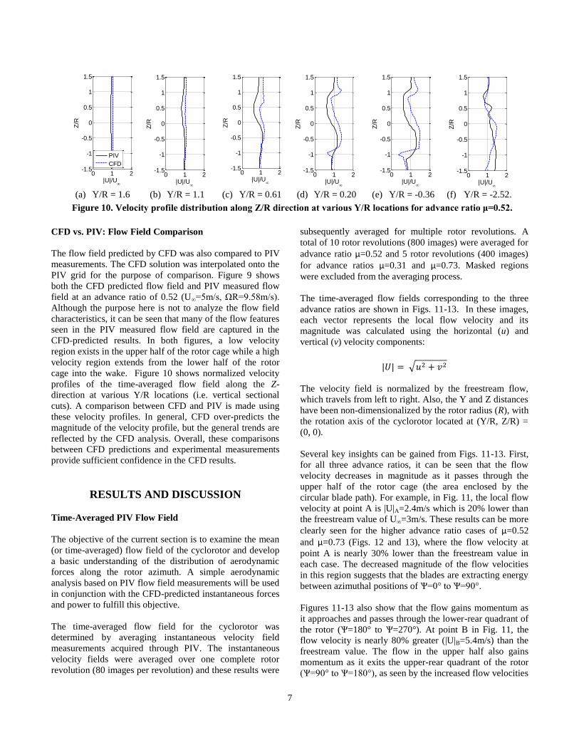
(a) Y/R = 1.6 (b) Y/R = 1.1 (c) Y/R = 0.61 (d) Y/R = 0.20 (e) Y/R = -0.36 (f) Y/R = -2.52.

Figure 10. Velocity profile distribution along Z/R direction at various Y/R locations for advance ratio μ=0.52.

CFD vs. PIV: Flow Field Comparison

The flow field predicted by CFD was also compared to PIV

measurements. The CFD solution was interpolated onto the

PIV grid for the purpose of comparison. Figure 9 shows

both the CFD predicted flow field and PIV measured flow

field at an advance ratio of 0.52 (U∞=5m/s, ΩR=9.58m/s).

Although the purpose here is not to analyze the flow field

characteristics, it can be seen that many of the flow features

seen in the PIV measured flow field are captured in the

CFD-predicted results. In both figures, a low velocity

region exists in the upper half of the rotor cage while a high

velocity region extends from the lower half of the rotor

cage into the wake. Figure 10 shows normalized velocity

profiles of the time-averaged flow field along the Z-

direction at various Y/R locations (i.e. vertical sectional

cuts). A comparison between CFD and PIV is made using

these velocity profiles. In general, CFD over-predicts the

magnitude of the velocity profile, but the general trends are

reflected by the CFD analysis. Overall, these comparisons

between CFD predictions and experimental measurements

provide sufficient confidence in the CFD results.

RESULTS AND DISCUSSION

Time-Averaged PIV Flow Field

The objective of the current section is to examine the mean

(or time-averaged) flow field of the cyclorotor and develop

a basic understanding of the distribution of aerodynamic

forces along the rotor azimuth. A simple aerodynamic

analysis based on PIV flow field measurements will be used

in conjunction with the CFD-predicted instantaneous forces

and power to fulfill this objective.

The time-averaged flow field for the cyclorotor was

determined by averaging instantaneous velocity field

measurements acquired through PIV. The instantaneous

velocity fields were averaged over one complete rotor

revolution (80 images per revolution) and these results were

subsequently averaged for multiple rotor revolutions. A

total of 10 rotor revolutions (800 images) were averaged for

advance ratio μ=0.52 and 5 rotor revolutions (400 images)

for advance ratios μ=0.31 and μ=0.73. Masked regions

were excluded from the averaging process.

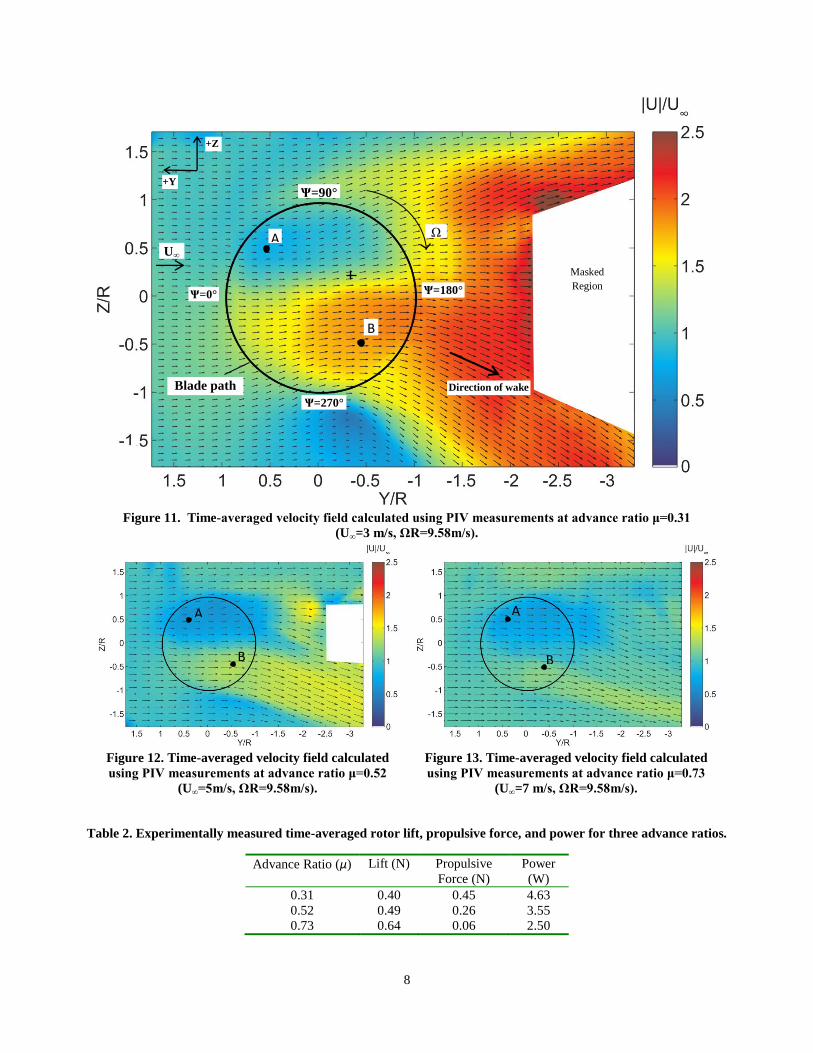
The time-averaged flow fields corresponding to the three

advance ratios are shown in Figs. 11-13. In these images,

each vector represents the local flow velocity and its

magnitude was calculated using the horizontal (u) and

vertical (v) velocity components:

√

The velocity field is normalized by the freestream flow,

which travels from left to right. Also, the Y and Z distances

have been non-dimensionalized by the rotor radius (R), with

the rotation axis of the cyclorotor located at (Y/R, Z/R) =

(0, 0).

Several key insights can be gained from Figs. 11-13. First,

for all three advance ratios, it can be seen that the flow

velocity decreases in magnitude as it passes through the

upper half of the rotor cage (the area enclosed by the

circular blade path). For example, in Fig. 11, the local flow

velocity at point A is |U|A=2.4m/s which is 20% lower than

the freestream value of U∞=3m/s. These results can be more

clearly seen for the higher advance ratio cases of μ=0.52

and μ=0.73 (Figs. 12 and 13), where the flow velocity at

point A is nearly 30% lower than the freestream value in

each case. The decreased magnitude of the flow velocities

in this region suggests that the blades are extracting energy

between azimuthal positions of Ѱ=0° to Ѱ=90°.

Figures 11-13 also show that the flow gains momentum as

it approaches and passes through the lower-rear quadrant of

the rotor (Ѱ=180° to Ѱ=270°). At point B in Fig. 11, the

flow velocity is nearly 80% greater (|U|B=5.4m/s) than the

freestream value. The flow in the upper half also gains

momentum as it exits the upper-rear quadrant of the rotor

(Ѱ=90° to Ѱ=180°), as seen by the increased flow velocities

0 1 2-1.5

-1

-0.5

0

0.5

1

1.5

|U|/U

Z/R

PIV

CFD

0 1 2-1.5

-1

-0.5

0

0.5

1

1.5

|U|/U

Z/R

0 1 2-1.5

-1

-0.5

0

0.5

1

1.5

|U|/U

Z/R

0 1 2-1.5

-1

-0.5

0

0.5

1

1.5

|U|/U

Z/R

0 1 2-1.5

-1

-0.5

0

0.5

1

1.5

|U|/U

Z/R

0 1 2-1.5

-1

-0.5

0

0.5

1

1.5

|U|/U

Z/R

8

Figure 11. Time-averaged velocity field calculated using PIV measurements at advance ratio μ=0.31

(U∞=3 m/s, ΩR=9.58m/s).

Figure 12. Time-averaged velocity field calculated

using PIV measurements at advance ratio μ=0.52

(U∞=5m/s, ΩR=9.58m/s).

Figure 13. Time-averaged velocity field calculated

using PIV measurements at advance ratio μ=0.73

(U∞=7 m/s, ΩR=9.58m/s).

Table 2. Experimentally measured time-averaged rotor lift, propulsive force, and power for three advance ratios.

Advance Ratio (μ) Lift (N) Propulsive

Force (N)

Power

(W)

0.31 0.40 0.45 4.63

0.52 0.49 0.26 3.55

0.73 0.64 0.06 2.50

Ѱ=0° Ѱ=180°

°

Ѱ=270°

°

U∞

Ω

+Z

+Y

Direction of wake

A

B

Ѱ=90°

°

Blade path

Masked

Region

A

B B

A

9

in the rotor wake. These observations imply that the blades

are adding energy to the flow in the rear half of the

cyclorotor. This is especially true in the lower-rear quadrant

(Ѱ=180° to Ѱ=270°), where the most significant increases

in local flow velocities are visible.

The net increase in momentum in the –Y-direction suggests

that the rotor is producing a positive net propulsive force.

Furthermore, the downward change in direction of the flow

in the rotor wake (Fig. 11(a)) corresponds to a net

momentum change in the Z-direction, which implies the

rotor is producing a net lift force. Together, these

observations for rotor lift and propulsive force are

confirmed by time-averaged performance measurements

presented in Table 2. For all three advance ratios, the rotor

produces positive lift and propulsive force. It is also evident

from Table 2 that the rotor power decreases with increasing

advance ratio; this is likely due to increased power

extraction by the blades between Ѱ=0° to Ѱ=90°.

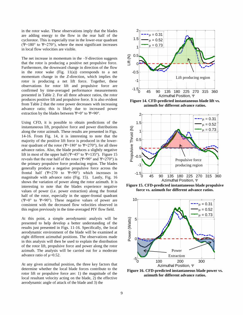
Using CFD, it is possible to obtain predictions of the

instantaneous lift, propulsive force and power distributions

along the rotor azimuth. These results are presented in Figs.

14-16. From Fig. 14, it is interesting to note that the

majority of the positive lift force is produced in the lower-

rear quadrant of the rotor (Ѱ=180° to Ѱ=270°), for all three

advance ratios. Also, the blade produces a slightly negative

lift in most of the upper half (Ѱ=45° to Ѱ=135°). Figure 15

reveals that the rear half of the rotor (Ѱ=90° and Ѱ=270°) is

the primary propulsive force producing region. The blades

generally produce a negative propulsive force across the

frontal half (Ѱ=270 to Ѱ=90°) which increases in

magnitude with advance ratio (Fig. 15). Lastly, Fig. 16

shows the variation of power along the rotor azimuth. It is

interesting to note that the blades experience negative

values of power (i.e. power extraction) along the frontal

half of the rotor, especially in the upper-frontal quadrant

(Ѱ=0° to Ѱ=90°). These negative values of power are

consistent with the decreased flow velocities observed in

this region previously in the time-averaged PIV flow field.

At this point, a simple aerodynamic analysis will be

presented to help develop a better understanding of the

results just presented in Figs. 11-16. Specifically, the local

aerodynamic environment of the blade will be examined at

eight different azimuthal positions. The observations made

in this analysis will then be used to explain the distribution

of the rotor lift, propulsive force and power along the rotor

azimuth. The analysis will be carried out for a moderate

advance ratio of μ=0.52.

At any given azimuthal position, the three key factors that

determine whether the local blade forces contribute to the

rotor lift or propulsive force are: 1) the magnitude of the

local resultant velocity acting on the blade, 2) the effective

aerodynamic angle of attack of the blade and 3) the

Figure 14. CFD-predicted instantaneous blade lift vs.

azimuth for different advance ratios.

Figure 15. CFD-predicted instantaneous blade propulsive

force vs. azimuth for different advance ratios.

Figure 16. CFD-predicted instantaneous blade power vs.

azimuth for different advance ratios.

0 45 90 135 180 225 270 315 360-1.5

-1

-0.5

0

0.5

1

1.5

2

Azimuthal Position,

Lift (N

)

= 0.31

= 0.52

= 0.73

0 45 90 135 180 225 270 315 360-1.5

-1

-0.5

0

0.5

1

1.5

2

Azimuthal Position,

Pro

puls

ive T

hru

st (N

)

= 0.31

= 0.52

= 0.73

0 100 200 300-5

0

5

10

Azimuthal Position,

Pow

er

(Watts)

= 0.31

= 0.52

= 0.73

Lift producing region

Propulsive force

producing region

Power

Extraction

10

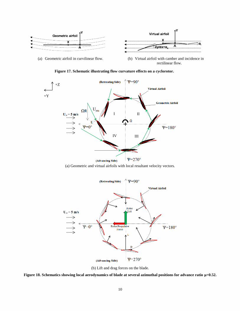
(a) Geometric airfoil in curvilinear flow. (b) Virtual airfoil with camber and incidence in

rectilinear flow.

Figure 17. Schematic illustrating flow curvature effects on a cyclorotor.

(a) Geometric and virtual airfoils with local resultant velocity vectors.

(b) Lift and drag forces on the blade.

Figure 18. Schematics showing local aerodynamics of blade at several azimuthal positions for advance ratio μ=0.52.

+Y

+Z

I II

III IV

11

orientation of the blade with respect to the freestream. The

magnitude and direction of the local resultant velocity

vector with respect to the blade chord line can be obtained

through a vector summation of the local flow velocity and

the blade tangential velocity:

For simplicity, the local flow vector will be assumed to be

in the direction of the freestream. The magnitude of the

local flow velocities at various azimuthal positions are

obtained using the mean flow field results from PIV.

The effective aerodynamic angle of attack of the blade is a

function of the geometric pitch angle (θ), the angle of attack

between the resultant velocity vector and the blade chord

line ( ), as well as an incidence angle ( ) which results

from flow curvature effects on the blade:

( )

Flow curvature effects on the blades of a cyclorotor result

from a chordwise variation of the local blade velocity,

which can be attributed to the orbital motion of the blades

(Ref. 23). These effects are discussed in detail in Ref. 4.

For the scope of this paper, it is sufficient to consider that

these flow curvature effects are due to a curvilinear flow

along the blade chord. Furthermore, a geometrically

symmetric airfoil immersed in a curvilinear flow can be

represented as a cambered airfoil in a rectilinear flow. This

is illustrated in Fig. 17. For the cyclorotor used in the

present study (R=3 in, c=1.95 in, c/R=0.65), a linear

approximation (Ref. 23) shows that the virtual camber is

approximately 8% of the blade chord. In addition, due to

the fact that the blade pitching axis is positioned at the

quarter-chord and not at the mid-chord, the blade

experiences a virtual incidence angle, which is

approximately 9° (calculated using the linear model in Ref.

23). Therefore, these values for camber and incidence

clearly suggest that flow curvature effects are not negligible

for the present cyclorotor. In order to account for flow

curvature effects in the current aerodynamic analysis, the

geometric airfoil is represented as a virtual airfoil that

features both camber and incidence angle.

The schematics presented in Fig. 18 are derived using the

aerodynamic analysis discussed above. Figure 18(a) shows

the blade at the eight different azimuthal positions

previously listed. Here, the camber line (red) corresponds to

the virtual airfoil and is superimposed on the geometric

airfoil. The local resultant velocity vectors acting on the

blade at each azimuthal position are also sketched (in

green). Note that these velocity vectors are drawn to scale,

based on the local flow velocity (U) and the blade

tangential velocity (ΩR). The local flow velocities (U) were

obtained using the PIV measured mean flow, as described

earlier in this section. Using the information provided in

Fig. 18(a), the directions of the local blade lift and drag

forces can be obtained and are shown in Fig. 18(b).

Together, the schematics in Fig. 18 will now be used to

explain the contributions of the local blade forces to the

overall rotor lift and propulsive force in various regions of

the rotor azimuth.

Region I (Ѱ=0° to Ѱ=90°): At Ѱ=0°, the effective angle of

attack of the blade is approximately zero, as depicted in Fig.

18(a). However, the blade is still expected to produce a lift

force due to its virtual camber. Based on the orientation of

the blade with respect to the freestream, the blade lift force

is expected to increase the net rotor lift, but decrease the net

propulsive force (Fig. 18(b)). The CFD-predicted results in

Figs. 14-15 support this finding, as they show negative

values for propulsive force and positive values for lift.

At Ѱ=45°, the blade operates with a slightly positive

effective angle of attack. However, the orientation of the

blade is such that the lift force acts to decrease both rotor

propulsive force and rotor lift. Furthermore, the blade

produces a force in the direction opposing the freestream

flow and as a result the incoming flow velocity is expected

to decrease across this region. This is consistent with the

observations made previously in the PIV flow field

measurements (Figs. 12). In reducing the flow velocities,

the blade extracts energy from the flow; this is evidenced

by the negative values of power observed in the CFD

results (Fig. 16).

Region II (Ѱ=90° to Ѱ=180°): At Ѱ=90°, the blade

operates with an increased effective angle of attack.

However, it is clear from Fig. 18(b) that the orientation of

the blade is such the majority of the blade lift force will be

in the Z-axis direction, which in turn decreases the net rotor

lift. This coincides with the negative values of lift observed

in this region from CFD predicted results (Fig. 14). It

should be noted, however, that the blade is in the retreating

half of the rotor in this region and therefore experiences

lower local resultant velocities. Thus, the decreases in net

rotor lift will be less pronounced.

At Ѱ=135°, the blade is at a slight positive effective angle

of attack. Based on the orientation of the blade in Fig.

18(b), the local lift force has components in the +Y-

direction and –Z-direction. Therefore, the blade increases

the net rotor propulsive force, but continues to decrease the

net rotor lift. It should be recalled that the local flow

velocities in this region are lower in magnitude due to the

power extraction by the blades in region I. Therefore, the

blade effective angle of attack in region II will be slightly

greater compared to region I.

Region III (Ѱ=180° to Ѱ=270°): At Ѱ=180°, the blade

has an increased effective angle of attack. The orientation

12

of the blade reveals that the blade contributes to both the

net rotor lift and propulsive force. It can be seen that the

contribution of the blade forces to the rotor propulsive force

will be maximum at an azimuthal location between Ѱ=135°

and Ѱ=180°, when its local lift vector becomes parallel to

the free stream. This observation is captured in the CFD-

predicted results in Fig. 15, where the maximum propulsive

force value occurs at approximately Ѱ=170°.

At Ѱ=225°, the blade experiences a large positive effective

angle of attack (Fig, 18(a)). Therefore, as shown in Fig.

18(b), the local aerodynamic forces on the blade are

significant. Furthermore, the orientation of the blade

suggests blade lift force will have components in the +Y-

and +Z-directions. Thus, the blade contributes to rotor

propulsive force and lift in this region.

Region IV (Ѱ=270° to Ѱ=0°): At Ѱ=270°, the blade is still

at a relatively large positive effective angle of attack. Fig.

18(b) shows that the majority of the blade lift force is along

the +Z-direction and therefore the primary contribution will

be to the rotor lift.

At Ѱ=315°, the blade is close to a zero effective angle of

attack. However the virtual camber allows the blade to

produce a non-zero local lift force, which has components

in the –Y- and +Z-directions. Thus, the blade still

contributes to the net rotor lift, but decreases the net

propulsive force in this region.

Effect of Advance Ratio

Although the above aerodynamic analysis was carried out

for one particular advance ratio (μ=0.52), the same general

principles were found to hold true for the lower and higher

advance ratios (μ=0.31 and μ=0.73) considered in this

study. However, the effective angle of attack distribution

of the blades along the rotor azimuth will be different due

to variations in the freestream velocity (constant Ω). From

the CFD results presented in Figs. 14-16, it can be seen that

the primary lift and propulsive force producing regions

remain relatively the same for the three different advance

ratios. Figure 16 shows that the effect of increasing advance

ratio is to increase the power extraction along the frontal

half of the rotor (Ѱ=270° to Ѱ=90°), whereas the power in

the rear half of the rotor azimuth remains relatively

constant. This is a key reason for the decrease in power

observed in the time-averaged experimental measurements

(Table 2).

The analysis just presented uses a simplified model, but it

effectively provides a fundamental understanding of the

physics behind the distribution of forces and power along

the rotor azimuth. These insights can assist with the design

of a rotor for a flight-capable cyclocopter MAV. For

example, asymmetric pitching kinematics, where one-half

of the rotor operates at a higher pitch angle than the

corresponding half, may help improve rotor propulsive

efficiency by leading to a more uniform azimuthal

distribution of forces (Ref. 24). Also, the idea of using

geometrically cambered airfoils for improving cyclorotor

performance may be worthwhile to consider.

Phase-Averaged PIV

Time-averaged PIV results provide insight into the mean

flow field of a cyclorotor, but do not show the effects of

unsteady aerodynamic flow features. The current section

uses phase-averaged PIV measurements to quantify

unsteady flow features and evaluate their impact on the

aerodynamic performance of the blades at specific

azimuthal positions.

As previously described, flow field measurements with high

temporal resolution were acquired using a time-resolved

PIV system. The sampling rate was 1.6 kHz and the rotor

operated at 20 Hz. This provided flow field measurements

at 80 azimuthal positions per rotor revolution (in 4.5°

increments). Of these 80 azimuthal positions, four pairs are

presented in this paper. Azimuthal positions can be paired

due to the symmetry of the two-bladed rotor, with the

blades denoted as blade A and blade B. For example, when

blade A is positioned at ѰA=0°, blade B is positioned at

ѰB=180°, etc. Instantaneous flow field measurements for

each pair of azimuthal positions were isolated from the data

set. The data set spanned 9.5 full rotor revolutions; images

were extracted for each rotor half-revolution (due to rotor

symmetry) giving 19 instantaneous flow field

measurements for each pair of azimuthal positions. These

measurements consist of two velocity components (in the Y-

and Z-directions). The instantaneous velocity components

for the 19 images at a single azimuthal position were then

averaged. Phase-averaging in this way highlights prominent

periodic flow features and reduces the appearance of

aperiodic effects in the flow.

In the following analysis, phase-averaged results will be

considered for the moderate advance ratio case of μ=0.52

(U∞=5 m/s, Ω=1200rpm). Emphasis is placed on the rear

half of the rotor azimuth, where the blades operate in the

wake of the frontal half and are therefore exposed to several

unsteady aerodynamic flow features (most notably, blade-

wake interactions).

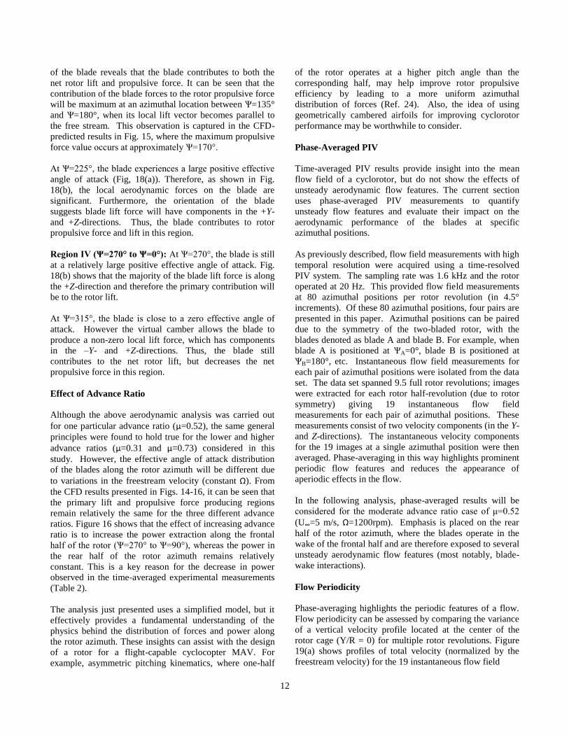
Flow Periodicity

Phase-averaging highlights the periodic features of a flow.

Flow periodicity can be assessed by comparing the variance

of a vertical velocity profile located at the center of the

rotor cage (Y/R = 0) for multiple rotor revolutions. Figure

19(a) shows profiles of total velocity (normalized by the

freestream velocity) for the 19 instantaneous flow field

13

(a) Velocity distribution along Z-axis at Y/R = 0.

(b) Instantaneous vorticity field.

(c) Phase-averaged vorticity field.

Figure 19. Comparison of instantaneous and phase-

averaged flow with blades at ѰA=0° and ѰB=180° (μ=0.52).

images (blue) as well as the final phase-averaged result

(red). For the data shown here, the blades are at azimuthal

locations of Ѱ=0° (rotor forward) and Ѱ=180° (rotor aft). In

general, the instantaneous velocity profiles show good

agreement; the aperiodicity of the flow is captured in the

deviations of the instantaneous velocity profiles from the

phase-averaged velocity profile. The effects of phase-

averaging on the flow field are illustrated in Fig. 19(b-c)

where an instantaneous vorticity field is compared with the

phase-averaged vorticity field. The instantaneous vorticity

field (Fig. 19(b)) reveals numerous discrete vortices,

especially in the upper-rear quadrant (Ѱ=90° to Ѱ=180°) of

the rotor. The phase-averaged vorticity field (Fig. 19(c))

appears more diffuse, which can be attributed to variations

in the spatial position and intensity of the vortices between

rotor revolutions. However, it can be seen that the phase-

averaged vorticity field more clearly shows the general

shape and trajectory of the blade wakes. A detailed

discussion on these blade wakes follows in the remainder of

this section.

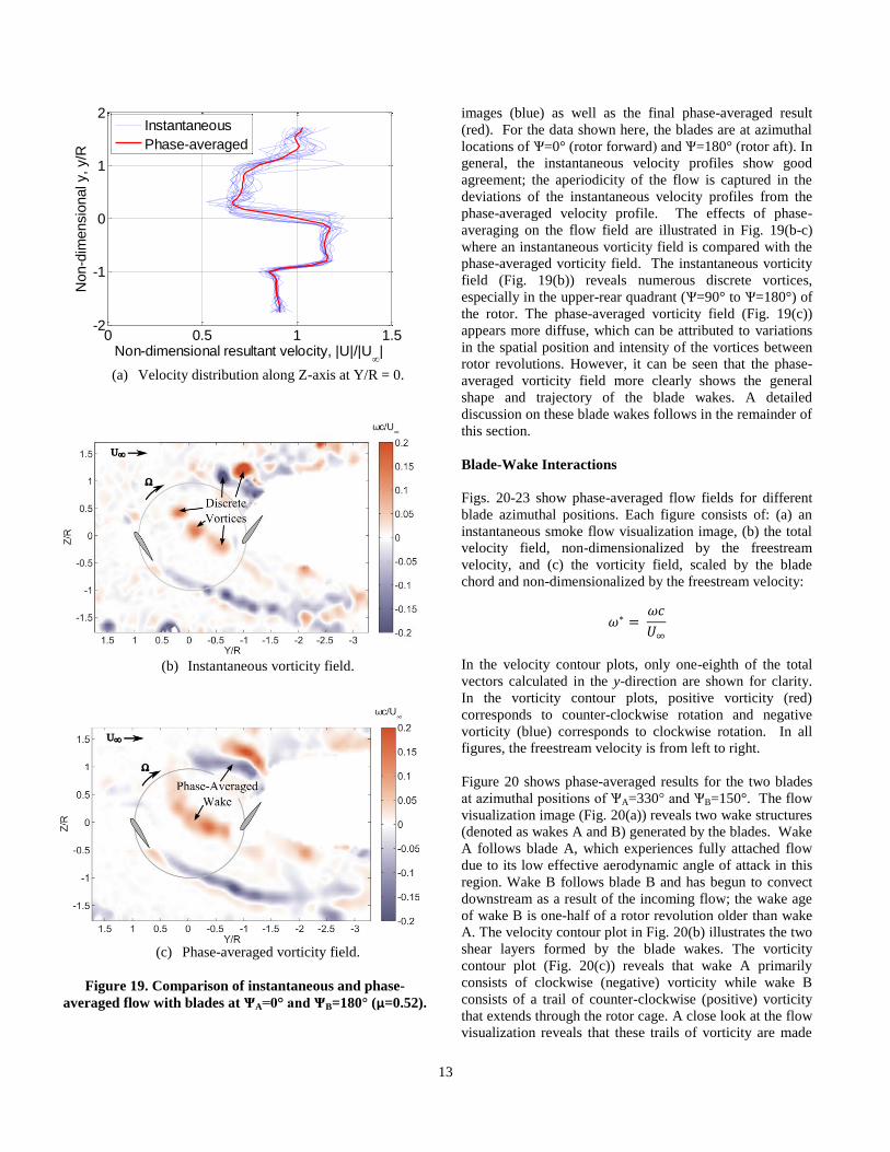
Blade-Wake Interactions

Figs. 20-23 show phase-averaged flow fields for different

blade azimuthal positions. Each figure consists of: (a) an

instantaneous smoke flow visualization image, (b) the total

velocity field, non-dimensionalized by the freestream

velocity, and (c) the vorticity field, scaled by the blade

chord and non-dimensionalized by the freestream velocity:

In the velocity contour plots, only one-eighth of the total

vectors calculated in the y-direction are shown for clarity.

In the vorticity contour plots, positive vorticity (red)

corresponds to counter-clockwise rotation and negative

vorticity (blue) corresponds to clockwise rotation. In all

figures, the freestream velocity is from left to right.

Figure 20 shows phase-averaged results for the two blades

at azimuthal positions of ѰA=330° and ѰB=150°. The flow

visualization image (Fig. 20(a)) reveals two wake structures

(denoted as wakes A and B) generated by the blades. Wake

A follows blade A, which experiences fully attached flow

due to its low effective aerodynamic angle of attack in this

region. Wake B follows blade B and has begun to convect

downstream as a result of the incoming flow; the wake age

of wake B is one-half of a rotor revolution older than wake

A. The velocity contour plot in Fig. 20(b) illustrates the two

shear layers formed by the blade wakes. The vorticity

contour plot (Fig. 20(c)) reveals that wake A primarily

consists of clockwise (negative) vorticity while wake B

consists of a trail of counter-clockwise (positive) vorticity

that extends through the rotor cage. A close look at the flow

visualization reveals that these trails of vorticity are made

0 0.5 1 1.5-2

-1

0

1

2

Non-dimensional resultant velocity, |U|/|U|

Non-d

imensio

nal y, y/R

Instantaneous

Phase-averaged

14

(a) Instantaneous flow visualization.

(b) Velocity field. (c) Vorticity field.

Figure 20. Phase-averaged flow field with blades at ѰA=330° and ѰB=150° (μ=0.52).

(a) Instantaneous flow visualization.

(b) Velocity field. (c) Vorticity field.

Figure 21. Phase averaged flow field with blades at ѰA=0° and ѰB=180° (μ=0.52).

15

(a) Instantaneous flow visualization.

(b) Velocity field. (c) Vorticity field.

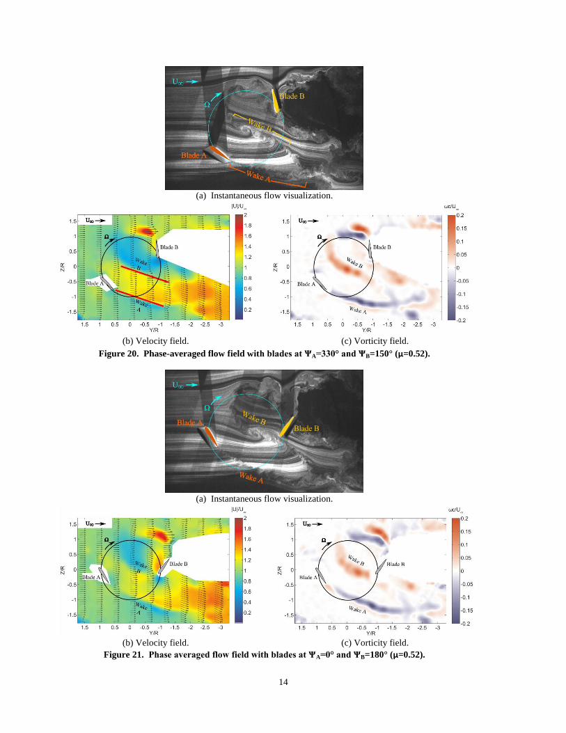
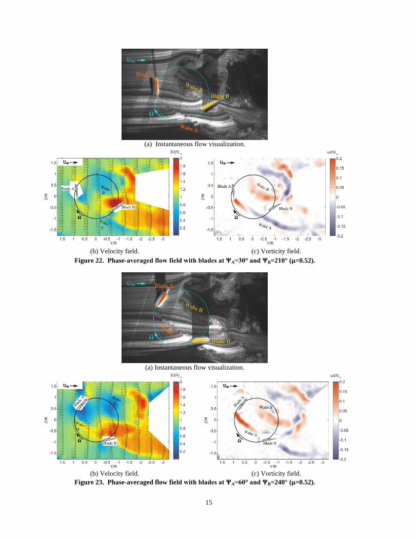
Figure 22. Phase-averaged flow field with blades at ѰA=30° and ѰB=210° (μ=0.52).

(a) Instantaneous flow visualization.

(b) Velocity field. (c) Vorticity field.

Figure 23. Phase-averaged flow field with blades at ѰA=60° and ѰB=240° (μ=0.52).

16

up of small-scale vortices, a result of a Kelvin-Helmoholtz

instability along each shear layer (Ref. 24). The rotation

direction of these vortices will become important when

evaluating the blade-wake interactions that take place as

blade B progresses further along the azimuth.

Figure 21 shows blades A and B advanced to azimuthal

positions of ѰA=0° and ѰB=180°. The flow visualization

image (Fig. 21(a)) shows the leading edge of blade B

approaching the trail of counter-clockwise vortices of wake

B. The velocity contour plot in Fig. 21(b) reveals a slightly

increased velocity region near the upper surface of blade B.

Figure 22 shows blades A and B advanced to ѰA=30° and

ѰB=210°. Here, a blade-wake interaction between the

upper surface of blade B and the counter-clockwise vortices

of wake B is evident. The velocity contours (Fig. 22(b))

show that this interaction acts to accelerate the flow over

the upper surface of blade B. It was shown in the previous

section that the blade operates with a positive effective

angle attack and experiences high dynamic pressure in this

region. These two characteristics, combined with the blade-

wake interaction act to accelerate the local flow velocity on

the upper surface of blade B to almost twice the freestream

value. Meanwhile, the flow near blade A is nearly

perpendicular to the blade chord. The flow downstream of

blade A is slowed (to the right and down of the blade in

Figure 22(b)); blade A is operating in a power extraction

region as discussed in the previous section. This prompts a

change in the direction of vorticity in the shear layer formed

in wake A, as evidenced by Fig. 22(c).

Figure 23 shows the blades at ѰA=60° and ѰB=240°. The

flow visualization image shows a second blade-wake

interaction, this time between blade B and the wake of

blade A, resulting in a high velocity region on the upper

surface of blade B (Fig. 23(b)). This region is slower than

the high velocity region associated with the first blade-wake

interaction. Analysis at higher blade azimuth resolution

would allow for more detailed description of the evolution

of each blade-wake interaction and is a topic for further

study.

It should be noted that the location and intensity of the

vortices along the wakes vary with each rotor revolution

due to the inherent aperiodicity of the flow. As a result, the

exact position of the blade-wake interactions observed in

Fig. 22-23 may vary slightly between revolutions.

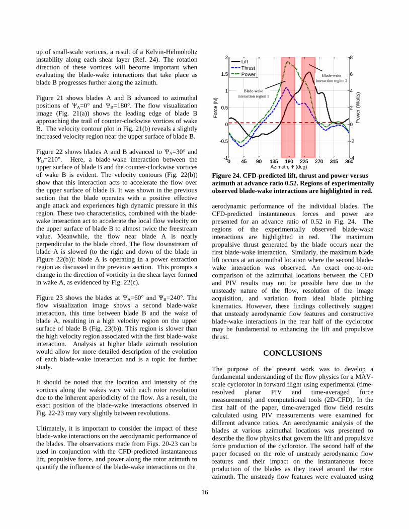
Ultimately, it is important to consider the impact of these

blade-wake interactions on the aerodynamic performance of

the blades. The observations made from Figs. 20-23 can be

used in conjunction with the CFD-predicted instantaneous

lift, propulsive force, and power along the rotor azimuth to

quantify the influence of the blade-wake interactions on the

aerodynamic performance of the individual blades. The

CFD-predicted instantaneous forces and power are

presented for an advance ratio of 0.52 in Fig. 24. The

regions of the experimentally observed blade-wake

interactions are highlighted in red. The maximum

propulsive thrust generated by the blade occurs near the

first blade-wake interaction. Similarly, the maximum blade

lift occurs at an azimuthal location where the second blade-

wake interaction was observed. An exact one-to-one

comparison of the azimuthal locations between the CFD

and PIV results may not be possible here due to the

unsteady nature of the flow, resolution of the image

acquisition, and variation from ideal blade pitching

kinematics. However, these findings collectively suggest

that unsteady aerodynamic flow features and constructive

blade-wake interactions in the rear half of the cyclorotor

may be fundamental to enhancing the lift and propulsive

thrust.

CONCLUSIONS

The purpose of the present work was to develop a

fundamental understanding of the flow physics for a MAV-

scale cyclorotor in forward flight using experimental (time-

resolved planar PIV and time-averaged force

measurements) and computational tools (2D-CFD). In the

first half of the paper, time-averaged flow field results

calculated using PIV measurements were examined for

different advance ratios. An aerodynamic analysis of the

blades at various azimuthal locations was presented to

describe the flow physics that govern the lift and propulsive

force production of the cyclorotor. The second half of the

paper focused on the role of unsteady aerodynamic flow

features and their impact on the instantaneous force

production of the blades as they travel around the rotor

azimuth. The unsteady flow features were evaluated using

Figure 24. CFD-predicted lift, thrust and power versus

azimuth at advance ratio 0.52. Regions of experimentally

observed blade-wake interactions are highlighted in red.

0 45 90 135 180 225 270 315 360-1

-0.5

0

0.5

1

1.5

2

Azimuth, (deg)

Forc

e (

N)

0 45 90 135 180 225 270 315 360-4

-2

0

2

4

6

8

Pow

er

(Watts)

Lift

Thrust

Power Blade-wake

interaction region 2

Blade-wake

interaction region 1

17

phase-averaged flow field measurements, with the blades at

selected azimuthal locations. Observations from this

analysis were correlated to CFD-predicted instantaneous

aerodynamic forces and power to understand the role of

blade-wake interactions in the generation of lift and

propulsive force by a cyclorotor.

The key conclusions from this study can be summarized as

follows:

1. The flow velocity decreases in magnitude as it

passes across the upper-frontal quadrant (Ѱ=0° to

Ѱ=90°) of the cyclorotor. This is attributed to

power extraction by the blades in this region. The

effect of increasing advance ratio is to increase

power extraction in the frontal half.

2. The primary force producing region of the

cyclorotor lies in the lower-aft region of the rotor

azimuth (Ѱ=180° to Ѱ=270°). An aerodynamic

analysis based on PIV time-averaged flow field

measurements revealed the blades operate in a

high dynamic pressure environment with a high

effective angle of attack. The significant

momentum addition by the blades in this region

results in high flow velocity across the lower half

of the rotor cage.

3. Constructive blade-wake interactions appear to

play an important role in enhancing the lift and

propulsive force generation of the blades in the

rear half of the rotor azimuth between Ѱ=150° and

Ѱ=270°. Specifically, the downstream blade

encounters two blade-wake interactions: one with

its own wake and another with the wake of the

upstream blade. The rotational flow induced by the

vortices located along the blade wakes accelerates

the flow over the upper surface of the blade.

ACKNOWLEDGEMENTS

This research was supported by the Army’s MAST CTA

Center for Microsystem Mechanics with Dr. Brett Piekarski

(Army Research Lab) and Mr. Chris Kroninger (Army

Research Lab – Vehicle Technology Directorate) as

Technical Monitors. Authors would like to thank Professor

Allen Winkelmann for providing use of the wind tunnel

facilities at the University of Maryland.

REFERENCES

1Pines, D., and Bohorquez, F., “Challenges Facing Future

Micro-Air-Vehicle Development," Journal of Aircraft, Vol.

43 (2), March/April 2006, pp. 290-305.

2Chopra, I., "Hovering Micro Air Vehicles: Challenges and

Opportunities," Proceedings of American Helicopter

Society Specialists' Conference, International Forum on

Rotorcraft Multidisciplinary Technology, October 15-17,

2007, Seoul, Korea.

3Benedict, M., Jarugumilli, T., and Chopra, I.,

"Experimental Investigation of the Effect of Rotor

Geometry and Blade Kinematics on the Performance of a

MAV-Scale Cycloidal Rotor," Proceedings of the American

Helicopter Society Specialists' Meeting on Unmanned

Rotorcraft and Network Centric Operations, Tempe, AZ,

January 25-27, 2011.

4Benedict, M., Jarugumilli, T., Lakshminarayan, V., K., and

Chopra, I., “Experimental and Computational Studies to

Understand the Role of Flow Curvature Effects on the

Aerodynamic Performance of a MAV-Scale Cycloidal

Rotor in Forward Flight,” Proceedings of the 53rd

AIAA/ASME/ASCE/AHS/ASC Structures, Structural

Dynamics, and Materials Conference, Honolulu, Hawaii,

April 23-26, 2012.

5Jarugumilli, T., Benedict, M., and Chopra, I.,

“Experimental Investigation of the Forward Flight

Performance of a MAV-scale Cycloidal Rotor,”

Proceedings of the 68th

Annual Forum of the American

Helicopter Society, Fort Worth, TX, May 1–3, 2012.

6Kirsten, F. K., “Cycloidal Propulsion Applied to Aircraft,”

Transactions of the American Society of Mechanical

Engineers, Vol. 50, No. AER-50-12, 1928, pp 25-47.

7Wheatley, J. B. and Windler, R., “Wind-Tunnel Tests of a

Cyclogiro Rotor,” NACA Technical Notes No. 528, May

1935.

8Eastman, F., Cottas, N., Barkheines, G., “Wind Tunnel

Tests on a High Pitch Cyclogyro,” University of

Washington Aeronautical Laboratory Report 191-A, 1943.

9Nagler, B., “Improvements in Flying Machines Employing

Rotating Wing Systems,” United Kingdom Patent No.

280,849, issued Nov. 1926.

10

Yun, C. Y., Park, I. K., Lee, H. Y., Jung, J. S., Hwang, I.

S., and Kim, S. J., “Design of a New Unmanned Aerial

Vehicle Cyclocopter,” Journal of American Helicopter

Society, Vol. 52, (1), January 2007, pp. 24–35.

18

11Hwang, I. S., Hwang, C. P., Min, S. Y., Jeong, I. O., Lee,

C. H., Lee., Y. H. and Kim, S. J., “Design and Testing of

VTOL UAV Cyclocopter with 4 Rotors,” Proceedings of

the 62nd Annual Forum of the American Helicopter

Society, Phoenix, AZ, April 29-May 1, 2006.

12

Iosilevskii, G., and Levy, Y., “Experimental and

Numerical Study of Cyclogiro Aerodynamics,” AIAA

Journal, Vol. 44, (12), 2006, pp 2866–2870.

13

Benedict, M., “Fundamental Understanding of the

Cycloidal-Rotor Concept for Micro Air Vehicle

Applications” Ph.D. Thesis, University of Maryland,

College Park, MD December 2010.

14

Lakshminarayan, V. K., “Computational Investigation of

Micro-Scale Coaxial Rotor Aerodynamics in Hover,” Ph.D.

dissertation, Department of Aerospace Engineering,

University of Maryland at College Park, 2009.

15

Pulliam, T., and Chaussee, D., “A Diagonal Form of an

Implicit Approximate Factorization Algorithm,” Journal

ofComputational Physics, Vol. 39, (2), February 1981, pp.

347–363.

16

Van Leer B., “Towards the Ultimate Conservative

Difference Scheme V. A Second-Order Sequel To

Godunovs Method, Journal of Computational Physics, Vol.

135, No. 2, 1997, pp. 229-248.

17

Roe, P., “Approximate Riemann Solvers, Parameter

Vectors and Difference Schemes,” Journal of

Computational Physics, Vol. 135, No. 2, 1997, pp. 250-258.

18

Koren, B., “Multigrid and Defect Correction for the

Steady Navier-Stokes Equations”, Proceedings of the 11th

International Conference on Numerical Methods in Fluid

Dynamics , Willamsburg, VA, June 1988.

19

Turkel, E., “Preconditioning Techniques in Computational

Fluid Dynamics,” Annual Review of Fluid Mechanics, Vol.

31, 1999, pp. 385–416

20

Spalart, P. R., and Allmaras, S. R., “A One-equation

Turbulence Model for Aerodynamic Flows,” AIAA Paper

1992-0439, 30th AIAA Aerospace Sciences Meeting and

Exhibit, Reno, NV, January 6–9, 1992.

21

Lee, Y., “On Overset Grids Connectivity and Automated

Vortex Tracking in Rotorcraft CFD,” Ph.D. Dissertation,

Department of Aerospace Engineering, University of

Maryland at College Park, 2008.

22

Migliore, P.G., Wolfe, W.P., and Fanuccif, J.B., “Flow

Curvature Effects on Darrieus Turbine Blade

Aerodynamics,” Journal of Energy, Vol. 4, (2), 1980, pp.

49-55.

23

Jarugumilli, T., Benedict, M., and Chopra, I.,

“Performance and Flow Visualization Studies to Examine

the Role of Pitching Kinematics on MAV-scale Cycloidal

Rotor Performance in Forward Flight,” Presented at the

AHS International Specialist’s Meeting on Unmanned

Rotorcraft, Scottsdale, AZ, January 22-24, 2013.

24

White, F. M., Viscous Fluid Flow. 3rd

ed. McGraw-Hill

International Edition, 2006.