Comparison of experimental and Computational Fluid

1

Comparison of experimental and Computational Fluid Dynamics (CFD) studies of severe slugging on an S-shaped vertical riser

D.A. Corredor

Chemical Engineering Department, Universidad de los Andes, Bogotá, Colombia

General Objective

• Model in CFD an S-‐shaped riser with a two-‐phase oil-‐air flow.

Specific Objectives

• To model a 3D S-‐shaped riser with a two-‐phase oil-‐air flow on STAR-‐CCM+ CFD software for six cases.

• To compare and validate experimental data from NTNU with the numerical CFD results.

• To present a comprehensive analysis of the data obtained through the CFD software and propose valid conclusions.

.

2

Comparison of experimental and Computational Fluid Dynamics (CFD) studies of severe slugging on S-shaped vertical riser

D.A. Corredor

Chemical Engineering Department, Universidad de los Andes, Bogotá, Colombia

Abstract

This article presents a Computational Fluid Dynamics (CFD) simulation of a two-‐phase oil-‐air flow on an s-‐shaped riser for the study of severe slugging. For the development of this simulation, the CFD program used was STAR-‐CCM+ with the Volume Of Fluid model (VOF) on an s-‐shaped pipe with a 50 mm internal diameter and 30.4 m of length. The simulations were ran at six different gas and liquid superficial velocities to validate the mean maximum and mean minimum pressure as well as the pressure time series obtained with the experimental data obtained by NTNU (Norway). For each of the simulations an orthogonal butterfly mesh was used with a total of 576.000 cells. The relative error was calculated for each of the six cases and had maximum values of 16.5 % for the mean maximum pressure and an 8.2 % for the mean minimum pressure for low gas superficial velocities, indicating that the simulation is better suited for predicting the mean maximum and minimum pressure at high gas superficial velocity.

Key words: CFD, severe slugging, two-‐phase, s-‐shaped riser.

1. Introduction

The oil industry is one of the pillars of today’s world economy, it provides the fuel that powers our principal ways of transportation, our industry and it is the raw material for hundreds of thousands of products across all consumer needs; summing up it is the most important resource on the planet on present times. Due to its high demand and the exhaustion of viable oil extraction sites in-‐land, the oil industry has begun exploring and exploiting off-‐shore; this has posed many design and operation challenges that have yet to be fully studied and understood.

Offshore oil production pipelines, known as risers, when operating on normal conditions with a two-‐phase flow, as in gas/oil, develop a very common flow pattern called severe slugging. Severe slugging is a transient multiphase flow phenomenon that occurs inside the riser pipeline where fast moving liquid slugs form; these liquid slugs carry high kinetic energy and introduce strong oscillating pressure, which can be potentially hazardous for the riser structure and for the processing facilities downstream. There are four steps in severe slugging; 1) slug generation, 2) slug production, 3) bubble penetration and 4) gas blowdown, these are illustrated on Figure 1. Severe slugging occurs when stratified flow

3

occurs in the flowline, and the ratio of gas to liquid flowrate is below some critical value such that the rate of pressure build-‐up upstream of the blockage at the riser base is insufficient to overcome the increase in hydrostatic head as the slug grows in the riser. (BP, 1994)

There are two recognizable severe slugging modes on s-‐shaped risers identified by (Park and Nydal, 2014) which are as follows:

• Severe Slugging-‐I (SS-‐I): Full blockage by liquid at the bottom bend of the first riser, with liquid penetrating some distance into the upstream flowline during the slug-‐generation period.

• Severe Slugging-‐II (SS-‐II): Partial blockage by liquid at the bend of the first riser, with gas passing through the bend also during the slug-‐generation period.

• Stable Flow: Nearly constant inlet pressure and no apparent slug buildup, which essentially means that steady hydrodynamic slug flow is in the riser. Small oscillating flow without the apparent characteristics of severe slugging is defined here as the stable flow.

Figure 1. Severe slugging phenomenon steps. (Park and Nydal, 2014)

Due to the substantially higher pressure drop that accompanies severe slugging in comparison with other flow patterns (Figure 2), irregular liquid and gas flow output ensues, this poses a great challenge on the operation of the system. For the optimal design, safety and performance of two-‐phase flow systems, it is necessary to understand the behavior and properties of severe slugging to expect on any given flow system conditions.

Figure 2 shows five types of two-‐phase flow regimes present on vertical pipes, which form at different flow conditions and pipe inclinations. These flow regimes possess distinct volume fraction distributions and introduce pressure fluctuations on pipelines.

4

Figure 2. Different types of flow regimes on vertical pipes. (Kippax, 2011)

There are two different approaches in the study of the slug flow: i) the experimental approach, which involves the construction of scale models of the desired riser geometry. This is equipped with flow sensors (i.e. wire mesh sensors (WMS)) to obtain data on the flow regimes present on the pipeline and the subsequent operation of the system on different conditions; and ii) the Computational Fluid Dynamics (CFD) approach where a numerical model of the riser system is constructed and tested in a wide range of conditions. Since the experimental approach provides solid results on the behavior of flow regimes but lacks the multiplicity of conditions in which a CFD can operate, both approaches are ultimately best used in conjunction (Abulkadir et al., 2015).

In this work, severe slugging behavior and characterization found in CFD simulations is validated using experimental data provided by the NTNU (Norges Teknisk-‐naturvitenskapelige Universitet, the Norwegian University of Science and Technology).

2. Bibliographic Review

This review focused on both areas of two-‐phase flow; i) S-‐shaped risers and ii) severe slugging; this was performed to determine the variables involved, not only in the structure of the oil pipeline, but in the hydrodynamics of the two-‐phase flow and the severe slugging such as the work methodology, approximations and considerations involved among others.

2.1 State of the Art

2.1.1 Experimental Research

5

Table 1 shows the experimental research performed on recent years on the matter of experimental studies of two-‐phase flow in pipes.

Table 1. Experimental research from recent years.

Author Objective Results/Conclusions López Tinoco, 2006 Severe slug flow characterization

on vertical risers of hydrocarbon producing systems.

Mass balance, momentum balance. Equations were used to characterize the conditions of a severe slugging phenomenon on vertical risers.

Vallée et al., 2008

Experimental investigation and CFD simulation of horizontal stratified two-‐phase flow phenomena.

The HAWAC test facility provides well defined analysis as well as variable boundary conditions, which allow very good CFD-‐code validation possibilities.

Meglio et al.,2012 Stabilization of slugging in oil production facilities with or without upstream pressure sensors.

Positive results of the model-‐based control solutions would probably be attenuated during real-‐scale implementations. In particular the model may not be representative for a large range of operating points on a real well, where inflows depend on bottom pressure, whereas they are assumed constant by the model.

Li N. et al., 2013 Gas-‐Liquid two-‐phase flow patterns in a pipeline-‐riser system with an S-‐shaped riser. 50 mm i.d. , horizontal pipeline with 114 m in length, followed by a 16 m downward inclined section and ended at an S-‐shaped flexible raiser.

Four types of flow patterns, severe slugging type 1 and 2, transition flow and stable flow. The S-‐shaped riser has a stabilizing effect on severe slugging at high liquid and gas velocities, reducing the region of unstable flow. The unstable region was over predicted by the stability criteria, which were originally developed for vertical risers. An existing model was modified by taking into consideration the gas blocked in the downcomer riser, which tested against experimental data showed a good performance.

Castillo et al., 2013

Experimental characterization of severe slug flow on inclined-‐vertical risers with 5 pressure transducers and 2 conductive ring probes.

When operating on high superficial liquid or gas velocities, severe slug flow frequency is bigger. Superficial gas and liquid velocities have great influence on the shape of severe slug

6

flow. The inclination of the angle of the pipeline has also influence on the form and development of the severe slug flow.

Diaz et al., 2014 Comparison of experimental and CFD studies of slug flow with viscous liquids in s-‐shaped riser.

The air-‐oil flow reached the stable behavior at lower air superficial velocities than the air-‐water case. Comparison between simulation and experimental results showed better agreement for low viscosity fluid, while for high viscosity fluid, the simulation predicted the pressure amplitude and the cycle period of the slugs.

Park and Nydal, 2014 Study on severe slugging in an S-‐Shaped riser: small scale experiments compared with simulations

Two main modes of severe slugging are observed visually, full blocking in the bend and partially blocking in the bend. OLGA simulations compare quite well with the experimental results. The differenes are within a 5 and 9% on the pressure amplitudes. The deviations on the slug periods are largest at low flow rates.

Abulkadir et al., 2015 Comparison of experimental and CFD studies of slug flow in a vertical riser (6 m vertical pipe with a 0.067 m internal diameter).

At steady-‐state, both the CFD and experiment predict similar behaviors. The slug behavior can be considered fully developed at 4.0 m. A reasonably good agreement between CFD and experiment was obtained, CFD simulation can be used to characterize slug flow parameters with a good level of confidence.

Azevedo et al., 2015 Linear stability analysis for severe slugging in air-‐water systems considering different choking mechanisms.

Continuity equations for gas and liquid phases, simplified mixture momentum equation, inertia neglecting (NPW, no pressure wave model)

2.1.2 CFD Research

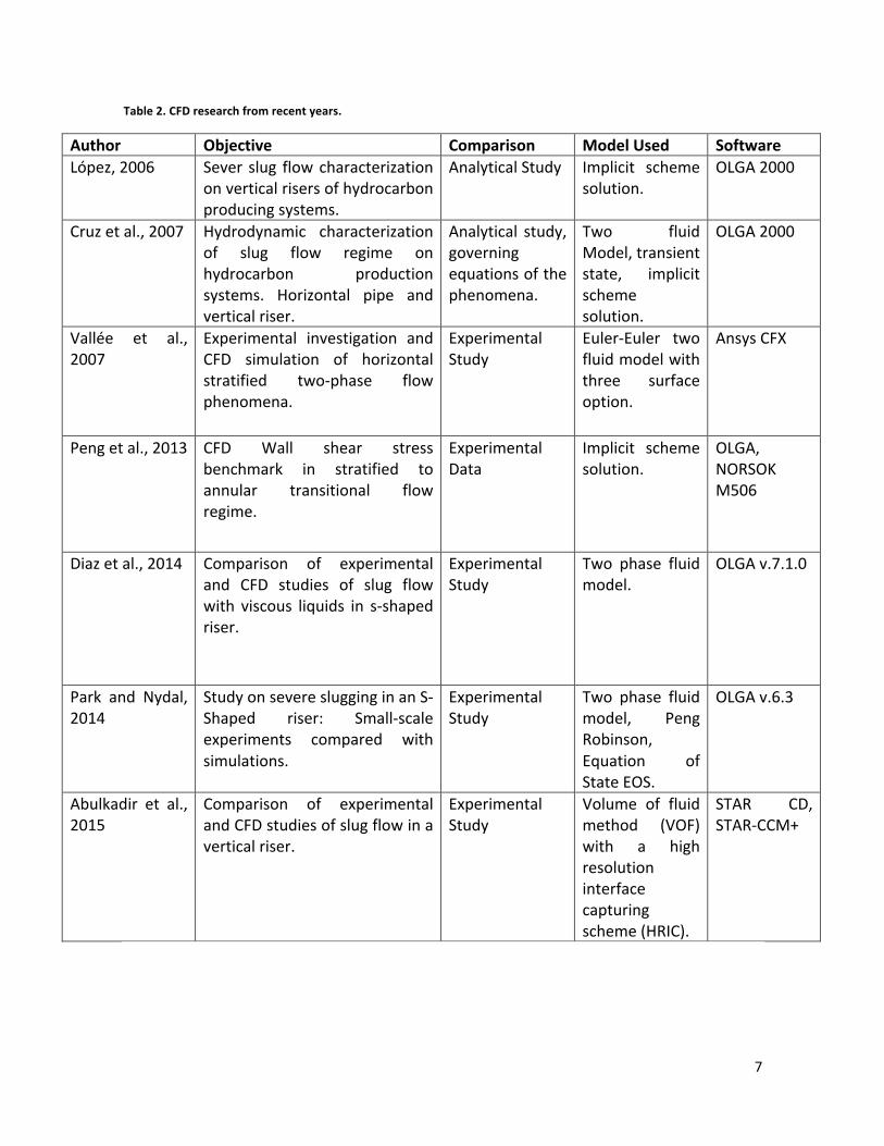
Table 2 shows the experimental research performed on recent years on the matter of CFD simulations of two-‐phase flow in pipes.

7

Table 2. CFD research from recent years.

Author Objective Comparison Model Used Software López, 2006 Sever slug flow characterization

on vertical risers of hydrocarbon producing systems.

Analytical Study Implicit scheme solution.

OLGA 2000

Cruz et al., 2007 Hydrodynamic characterization of slug flow regime on hydrocarbon production systems. Horizontal pipe and vertical riser.

Analytical study, governing equations of the phenomena.

Two fluid Model, transient state, implicit scheme solution.

OLGA 2000

Vallée et al., 2007

Experimental investigation and CFD simulation of horizontal stratified two-‐phase flow phenomena.

Experimental Study

Euler-‐Euler two fluid model with three surface option.

Ansys CFX

Peng et al., 2013 CFD Wall shear stress benchmark in stratified to annular transitional flow regime.

Experimental Data

Implicit scheme solution.

OLGA, NORSOK M506

Diaz et al., 2014 Comparison of experimental and CFD studies of slug flow with viscous liquids in s-‐shaped riser.

Experimental Study

Two phase fluid model.

OLGA v.7.1.0

Park and Nydal, 2014

Study on severe slugging in an S-‐Shaped riser: Small-‐scale experiments compared with simulations.

Experimental Study

Two phase fluid model, Peng Robinson, Equation of State EOS.

OLGA v.6.3

Abulkadir et al., 2015

Comparison of experimental and CFD studies of slug flow in a vertical riser.

Experimental Study

Volume of fluid method (VOF) with a high resolution interface capturing scheme (HRIC).

STAR CD, STAR-‐CCM+

8

3. Materials and methods

This work uses CFD simulations of severe slugging pattern to validate the pressure time series and mean maximum and minimum pressure, on section 1 (Annex A) of the simulation riser, results with experimental data obtained by the experimental facility at NTNU; the models, conditions and experimental correlations used in both simulation and experiment are explained below.

3.1 Experimental setup (NTNU)

The experimental data used to compare the simulation of the severe slugging phenomenon was obtained by the Energy and Process Technology Department at NTNU, which has an experimental facility that is capable of generating various flow patterns on the desired S-‐shaped riser geometry.

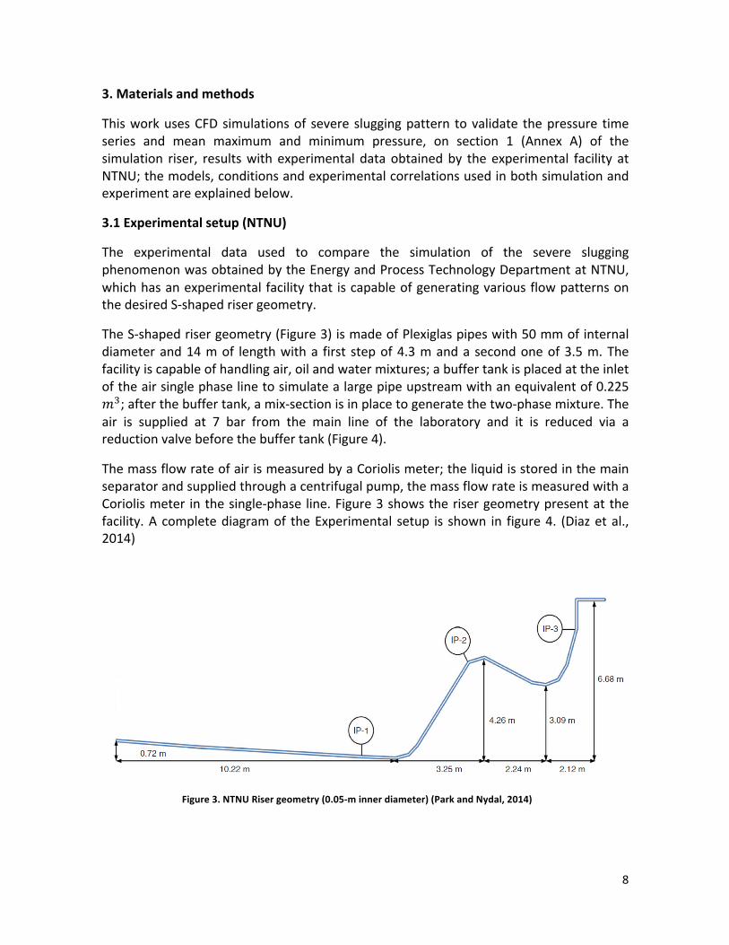
The S-‐shaped riser geometry (Figure 3) is made of Plexiglas pipes with 50 mm of internal diameter and 14 m of length with a first step of 4.3 m and a second one of 3.5 m. The facility is capable of handling air, oil and water mixtures; a buffer tank is placed at the inlet of the air single phase line to simulate a large pipe upstream with an equivalent of 0.225 𝑚!; after the buffer tank, a mix-‐section is in place to generate the two-‐phase mixture. The air is supplied at 7 bar from the main line of the laboratory and it is reduced via a reduction valve before the buffer tank (Figure 4).

The mass flow rate of air is measured by a Coriolis meter; the liquid is stored in the main separator and supplied through a centrifugal pump, the mass flow rate is measured with a Coriolis meter in the single-‐phase line. Figure 3 shows the riser geometry present at the facility. A complete diagram of the Experimental setup is shown in figure 4. (Diaz et al., 2014)

Figure 3. NTNU Riser geometry (0.05-‐m inner diameter) (Park and Nydal, 2014)

9

Riser

P

MAIN SEPARATOR

OIL LINE

WATER LINE

SMALL SEPARATOR

OVERFLOW TANK

LARGE CENTRIFUGAL PUMP

AIR LINE

BUFFER TANK

SMALL CENTRIFUGAL PUMP

LARGE FLOW METER

SMALL FLOW METER

AIR TANK 7 BAR

AIR TANK 4 BAR

Figure 4. NTNU Experimental facility setup. (Diaz et al., 2014)

3.2 CFD model

For the CFD model, the geometry of the S-‐shaped riser was created in a 3D environment in Autodesk Inventor Professional 2014 CAD with the dimensions specified in the NTNU paper; the governing equations, models and mesh generation were all generated using the STAR-‐CCM+ v 10.04.009 CFD software and are explained here.

Since the NTNU experiment was carried out with an air-‐oil mixture, standard values of viscosity, density and surface tension were used for each component shown in Table 3, at 298 K and 1 atm of pressure. All cases were run for a physical time of 105 s.

10

Table 3. Fluid properties of oil and air.

Fluid Oil Air Density [kg/m3] 831 1.2 Viscosity [cP] 60 0.02

Surface Tension [kN/m] 30

3.3.1 Geometry

For the simulation, a 3D model of the S-‐shaped riser was constructed in Autodesk Inventor based on the NTNU experimental facility dimensions, with a 50 mm diameter, 31.53 m length and 6.5 m height. The plan for the S-‐shaped riser is attached on Annex A.

An additional pipe was added before the riser in order to represent the buffer tank present in the experimental facility.

3.3.2 Superficial velocity

When working with two-‐phase flows and average velocity cannot be defined using only volumetric flow (𝑄) and cross sectional area (𝐴). This is due to the fact that the area occupied by a phase depends on time and location, which results in the volume flow not being proportional to speed. (Bratland, 2010) This velocity is a mathematical parameter used for analyzing two-‐phase flow. Gas superficial velocity is defined as shown in equation (2) and liquid superficial velocity in equation (3).

𝛼! =𝑉!𝑉 (1)

𝑣!" =𝑄(𝛼!)𝐴 (2)

𝑣!" =𝑄 1− 𝛼!

𝐴 (3)

Where 𝑣!" is the gas superficial velocity [m/s] , 𝑣!" is the liquid superficial velocity [m/s] and 𝛼! (equation (1)) is the void fraction; when 𝛼! = 0 the pipe is filled exclusively with liquid and when 𝛼! = 1 it is exclusively filled with gas.

3.3.3 Governing equations

Since the focus of this work is the study of a specific flow pattern that involves two different phases, the Navier-‐Stokes general transport equations are the main tools to study the severe slugging behavior. The differential form of this equation is given by equation (4).

𝜕(𝜌𝜙)𝜕𝑡 + 𝑑𝑖𝑣 𝜌𝜙𝒖 = 𝑑𝑖𝑣 Γ𝑔𝑟𝑎𝑑𝜙 + 𝑆! (4)

11

Which can be described as the rate of increase of 𝜙 of fluid element plus the net rate of flow of 𝜙 out of fluid element equal to the rate of increase of 𝜙 due to diffusion plus the rate of increase of 𝜙 due to sources respectively, where 𝜙 is a general property. (Malalasekera, 1995). STAR CCM+ solves the equation from its integral form using the finite volumes method, the equation is given by equation (5) which has to be integrated by time because of the transient nature of severe slugging.

𝜕𝜕𝑡

!!

( 𝜌𝜙𝑑𝑉)!"

𝑑𝑡 + 𝒏 𝜌𝜙𝒖 𝑑𝐴!

= 𝒏 Γ𝑔𝑟𝑎𝑑𝜙 𝑑𝐴 + 𝑆!𝑑𝑉!"!

(5)

The mass conservation equation (equation (6)) also needs to be considered when modeling two-‐phase flow.

𝜕𝜕𝑡 𝛼!𝜌!𝑥𝑑𝑉

!

+ 𝛼!𝜌!𝑥(!

v! − v!)𝑑𝑎 = 𝑚!" −𝑚!" 𝑎!"𝑥𝑑𝑉!!!

!

+ 𝑆!𝛼𝑑𝑉!

(6)

Where 𝛼! is the volume fraction of phase i, 𝜌! is the density of phase i, 𝑥 is the void fraction, v! is the velocity of phase i, v! is the grid velocity, 𝑚!" is the mass transfer rate to phase i from phase j (𝑚!" ≥ 0), 𝑚!" is the mass transfer rate to phase j from phase i (𝑚!" ≥ 0), 𝑎!" is the interaction area density and 𝑆!! is the phase mass source term.

3.3.4 Models used

A general overview of the most important models used for the simulation of the severe slugging phenomena in STAR-‐CCM+.

3.3.4.1 Volume of fluid model (VOF)

The volume of fluid (VOF) model is designed to capture the interface between two (or more) immiscible fluids. In this method, it is assumed that all phases share velocity, pressure and temperature hence the inter-‐phase interactions are not modeled. This model is suited for multiphase flows where two fluids (in this case liquid-‐gas) are clearly and separated (Soldan, 2013).

The VOF model description assumes that all immiscible fluid phases present in a control volume share velocity, pressure and temperature fields. Therefore, the same set of basic governing equations describing momentum, mass, and energy transport in a single-‐phase flow is solved.

The equations are solved for an equivalent fluid whose physical properties are calculated as function of the physical properties of its constituent phases and their volume fractions.

12

𝜌 = 𝛼!𝜌!

!

!!!

(7)

𝜇 = 𝛼!𝜇!

!

!!!

(8)

𝛼! =𝑉!𝑉 (9)

Where 𝛼! is the volume fraction and𝜌!, 𝜇! and 𝑐! ! are the density, molecular viscosity

and specific heat of the i th phase.

The conservation equation that describes the transport of volume fractions 𝛼! is:

𝑑𝑑𝑡 𝛼!𝑑𝑉 + 𝛼!(

!!v− v!) ∙ 𝑑a = 𝑆!! −

𝛼!𝜌!𝐷𝜌!𝐷𝑡 𝑑𝑉

! (10)

Where 𝑆!! is the source or sink of the ith phase, and !!!

!"is the material or Lagrangian

derivative of the phase densities 𝜌! (CD Adapco User Guide).

3.3.4.2 SST 𝒌− 𝝎 turbulence model

The SST 𝑘 − 𝜔 turbulence model solves two transport equations, these are solved for the turbulent kinetic energy 𝑘 and a quantity called 𝜔 which is defined as the specific dissipation rate, that is, the dissipation rate per unit turbulent kinetic energy (𝜔~𝜀/𝑘).

It is similar to the 𝑘 − 𝜀 models but presents a better performance when modeling separated flows, low-‐Reynolds number flows (transitional), near wall precision and sensible inlet boundary conditions (Yen, 2013).

One reported advantage of the 𝑘 − 𝜔 model over the 𝑘 − 𝜀 model is its improved performance for boundary layers under adverse pressure gradients, yet the most significant advantage is that it may be applied throughout the boundary layer, including the viscous-‐dominated region, without further modification (CD Adapco User Guide).

Severe slugging is an unsteady phenomenon that occurs at low gas and liquid rates, which translates into low-‐Reynolds number flow; this makes the election of the SST 𝑘 − 𝜔 turbulence model ideal for this simulation.

3.3.4.3 Gravity

For the gravity model, since the geometry was built on the Autodesk Inventor CAD software and a sweep function was used to create the pipe, the whole structure was tilted a few degrees; the solution to the tilt was solved by calculating the different components of gravity on the axes x and z.

13

3.3.4.4 Initial and boundary conditions

The initial conditions for the simulation replicate the conditions of the experiment carried out at NTNU where the riser starts completely full of liquid; the inlet was described as a velocity inlet and assigned a field function that divided it into two identical sections that represent the liquid and gas inlet. The outlet was described as a pressure outlet, a 1 atm pressure was assigned as a constant value and a 1 gas volume fraction to prevent reversed flow.

Table 4 contains the six pairs of gas and liquid superficial velocities assigned to each study case for this work.

Table 4. Study cases for CFD simulation

Case 𝒗𝑺𝑳 [m/s] 𝒔𝑺𝑮 [m/s] 1 0.1 1.1 2 0.1 2.3 3 0.1 5.6 4 0.2 1.4 5 0.2 3.0 6 0.2 5.6

3.3.4.5 Mesh generation

The CFD simulation software STAR-‐CCM+ uses a discretization of surfaces and volumes approach to solve the many models and physics phenomena that may apply, called the finite volume method. It divides a region of space into a discrete number of parts called cells, which simplify the calculation of the transport equations. The discretization as described before is called mesh generation and is of great importance when modeling any kind of physic phenomenon. This work simulates a two-‐phase flow, which requires of a special mesh design in order to obtain the most accurate results as evidenced in other studies (Abulkadir et al., 2015) called orthogonal meshing (also known as butterfly meshing).

Butterfly mesh has a characteristic design as shown in figure 4. It has two sections: i) a square shaped section that is located in the center of the pipe, it has a grid design; ii) it starts on the edge of the square grid and ends at the pipes cross section edge, forming a grid of consecutively rounded squares that finally reaches a completely circular shape as it reaches the edge.

The generation of the butterfly mesh in STAR-‐CCM+ was achieved by using the built-‐in feature called directed meshing.

14

Figure 4. Butterfly mesh.

3.3.4.5.1 Grid independence

For this study, three meshes where generated, a coarse, normal and fine mesh. The normal mesh was set to have a 3 mm wide cell on the grid section of the butterfly design. The coarse and refined where set to have a 30 % wider and slimmer cell on the grid section respectively, resulting in a 2 mm wide cell for the refined mesh and a 4 mm wide cell for the coarse mesh. The cell depth ∆𝑥 was defined with equation (11).

∆𝑥 = 𝐷 ∗ 0.3 (11)

Table 5 shows the number of cells on the cross section, number of sections and total number of cells.

Table 5. Mesh properties

Fine Mesh Normal Mesh Coarse Mesh Number of cells on cross section 605 320 180 Width of the cell [mm] 2.3 3.1 4 Number of sections 1800 1800 1800 Total number of cells 1,089,000 576,000 324,000

a) b) c)

Figure 5. a) Coarse, b) Normal, c) Fine meshes

15

The number of sections was not included in the study. The physical time used was 50 s on case 4.

3.3.4.6 Implicit unsteady model

The implicit transient model is used whenever a problem is time dependent, i.e. unsteady; it performs a time discretization to calculate the transport equations. Because of the transient nature of severe slugging, the implicit unsteady model was chosen.

In the Implicit Unsteady approach, each physical time-‐step involves some number of inner iterations to converge the solution for that given instant of time. These inner iterations can be accomplished using implicit spatial integration or explicit spatial integration schemes. A physical time-‐step size is specified that is used in the outer loop. The integration scheme marches inner iterations using optimal pseudo-‐time steps that are determined from the Courant number (CD Adapco User Guide).

The time step ∆𝑇 in which the physics equations are going to be calculated has to be small enough for the model to converge. For the convergence of the simulation the Courant-‐Friederich-‐Levy stability condition must be satisfied; the Courant number, for short, is defined as shown in equation (12), and must be lower than 1 to ensure convergence of the simulation.

𝐶 =𝑢!∆𝑇∆𝑥 (12)

Where 𝑢! is the Taylor bubble speed, ∆𝑇 is the time step and ∆𝑥 is the cell depth. To ensure that the convergence criterion is being satisfied, the time step is calculated.

A time step of 0.001 s was set for the simulation by monitoring the convective courant number on various sections of the riser and ensuring it satisfied the convergence condition.

4. Results and discussion

On this section, the results of the simulation cases and the analysis performed with simulation and NTNU experimental data are shown, as well as the grid sensibility study.

4.1 Grid independency study

The grid independency study was performed for case 4 (table 4) with a physical time of 50 s on a virtual machine running with 10 cores with windows 7 with an Intel ® Xeon® CPU E5-‐2695 v2 @ 2.40GHz processor with 64 GB of RAM memory. The targeted variables were the mean maximum and mean minimum pressure. The simulation error was calculated with equation (13).

𝑒𝑟𝑟𝑜𝑟 % =𝑎!"# − 𝑎!"#

𝑎!"#∗ 100 (13)

16

Table 6 shows the results of the grid sensibility study.

Table 6. Grid sensibility study results

Mesh Coarse Normal Refined Total cell number 324000 576000 1089000 Time [h] 105 144 292 meanMaxP Simulation [bar] 1.35 1.35 1.35 meanMaxP Experimental [bar] 1.62 meanMinP Simulation [bar] 1.26 1.23 1.25 meanMinP Experimental [bar] 1.18 meanMaxP Simulation Error [%] 16.33 16.5 16.4 meanMinP Simulation Error [%] 7.13 4.71 6.00

For the mean maximum pressure, all errors found for each mesh design are similar, changing only in the order of 10!! which indicates there is no meaningful difference and consequently a mesh design can not be chosen based on mean maximum pressure prediction accuracy.

For the mean minimum pressure, the lowest error is for the normal mesh design with a value of 4.71 %, the refined mesh is next with a 6% and finally the coarse mesh with a 7.13 %; this result shows the expected higher error for the coarse mesh, yet the normal mesh yields a lower error than the refined mesh.

These error values, while not meaningfully high for the mean minimum pressure, can be explained by the VOF model used to simulate the flow phenomena which requires the cells on the mesh design to have a certain size to capture the interface between the faces of the mixture as seen on figure 6.

Figure 6. a) Unsuitable grid b) Suitable grid for VOF model. (CD Adapco User Guide)

The normal mesh design was chosen to perform the simulations as it shows a good balance between error and computational time.

17

4.2 CFD simulation results

The simulations for the six cases proposed were run for a physical time of 105 s on a 10 cores machine. Figure 7 shows the residuals of the equations solved for case 4 (table 1). The graph shows a clear stabilization starting from iteration 4000 or 0.8 s all the way to iteration 500000 or 100 s which evidences the correct convergence of case 4 simulation.

Figure7. Residuals plot for case 4

All other cases show the same behavior on their residuals graphs, indicating all cases converged correctly.

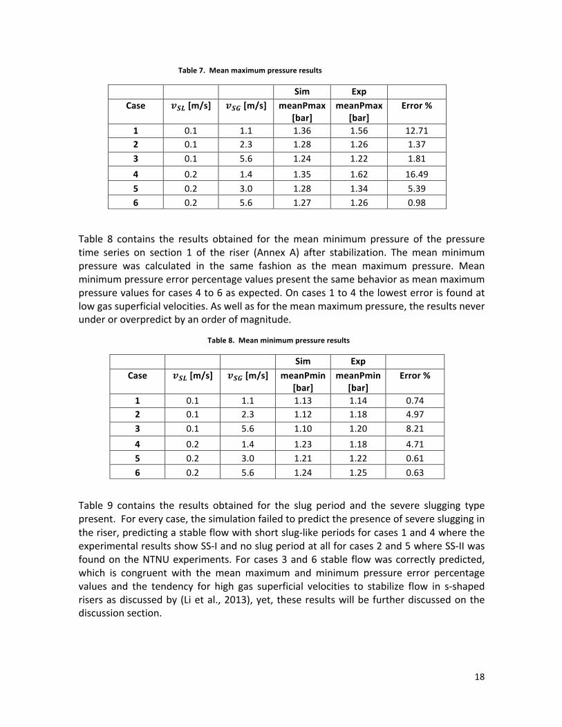
Table 7 contains the results obtained for the mean maximum pressure of the pressure time series on section 1 of the riser (Annex B) after stabilization. The mean maximum pressure was calculated by performing an average of the ten maximum pressure values of the pressure time series. The maximum error percentage values are found on cases 1 and 4 where the superficial gas and liquid velocities are at its lowest, reaching a significant peak value of 16% on case 4. The lowest error values belong to cases 3 and 6, indicating the simulation best predicts the mean maximum pressure for high gas superficial velocities and under predicts for low gas superficial velocities though never by an order of magnitude.

18

Table 7. Mean maximum pressure results

Sim Exp Case 𝒗𝑺𝑳 [m/s] 𝒗𝑺𝑮 [m/s] meanPmax

[bar] meanPmax

[bar] Error %

1 0.1 1.1 1.36 1.56 12.71 2 0.1 2.3 1.28 1.26 1.37 3 0.1 5.6 1.24 1.22 1.81 4 0.2 1.4 1.35 1.62 16.49 5 0.2 3.0 1.28 1.34 5.39 6 0.2 5.6 1.27 1.26 0.98

Table 8 contains the results obtained for the mean minimum pressure of the pressure time series on section 1 of the riser (Annex A) after stabilization. The mean minimum pressure was calculated in the same fashion as the mean maximum pressure. Mean minimum pressure error percentage values present the same behavior as mean maximum pressure values for cases 4 to 6 as expected. On cases 1 to 4 the lowest error is found at low gas superficial velocities. As well as for the mean maximum pressure, the results never under or overpredict by an order of magnitude.

Table 8. Mean minimum pressure results

Sim Exp Case 𝒗𝑺𝑳 [m/s] 𝒗𝑺𝑮 [m/s] meanPmin

[bar] meanPmin

[bar] Error %

1 0.1 1.1 1.13 1.14 0.74 2 0.1 2.3 1.12 1.18 4.97 3 0.1 5.6 1.10 1.20 8.21 4 0.2 1.4 1.23 1.18 4.71 5 0.2 3.0 1.21 1.22 0.61 6 0.2 5.6 1.24 1.25 0.63

Table 9 contains the results obtained for the slug period and the severe slugging type present. For every case, the simulation failed to predict the presence of severe slugging in the riser, predicting a stable flow with short slug-‐like periods for cases 1 and 4 where the experimental results show SS-‐I and no slug period at all for cases 2 and 5 where SS-‐II was found on the NTNU experiments. For cases 3 and 6 stable flow was correctly predicted, which is congruent with the mean maximum and minimum pressure error percentage values and the tendency for high gas superficial velocities to stabilize flow in s-‐shaped risers as discussed by (Li et al., 2013), yet, these results will be further discussed on the discussion section.

19

Table 9. Slug period and severe slugging type results

Sim Exp Sim Exp Case 𝒗𝑺𝑳 [m/s] 𝒗𝑺𝑮 [m/s] Period [s] Period [s] SS Type SS Type 1 0.1 1.1 4 69.04 S SI 2 0.1 2.3 0 24.63 S SII 3 0.1 5.6 0 0.00 S S 4 0.2 1.4 3.5 56.20 S SI 5 0.2 3.0 0 24.59 S SII 6 0.2 5.6 0 0.00 S S

Figure 8 presents the pressure time series for case 4 on section 1 (Annex B). The stable flow behavior predicted can be observed by the stabilization with small oscillations of the pressure and no apparent slug buildup. The experimental data shows the slug build-‐up period and the increase in pressure as the liquid phase starts to fill the first section of the riser; after, the gas blowdown is present where there is a sudden drop of pressure which is a characteristic inlet (section 1, Annex A) pressure behavior for SS-‐I.

Figure 8. Case 4 Pressure time series comparison.

Figures 9 and 10 show the mean maximum and minimum pressure results obtained with the simulation and the experimental results obtained at NTNU. For each liquid superficial velocity, the mean maximum pressure shows a descending tendency as the superficial gas velocity increases, overlapping with the experimental results. Pressure values for low gas superficial velocity are underpredicted by the simulation due to the fact that there are no liquid slugs forming and raising the pressure in the simulation. The mean minimum pressure also shows a similar increasing behavior as gas superficial velocity increases, overlapping too with the experimental results.

1

2

3

0 20 40 60 80 100

P [bar]

cme [s]

Simulanon

Experimental

20

Figure 9. Pressure time series for cases 1, 2 and 3 mean ax and min pressure comparison.

Figure 10. Pressure time series for cases 4, 5 and 6 mean ax and min pressure comparison.

1

1.1

1.2

1.3

1.4

1.5

1.6

1.7

1 1.5 2 2.5 3 3.5 4 4.5 5 5.5 6

P [bar]

vSG [m/s]

meanPmax Simulanon

meanPmax Experimental

meanPmin Simulanon

meanPmin Experimental

1

1.1

1.2

1.3

1.4

1.5

1.6

1.7

1 1.5 2 2.5 3 3.5 4 4.5 5 5.5 6

P [bar]

vSG [m/s]

meanPmax Simulanon

meanPmax Experimental

meanPmin Simulanon

meanPmin Experimental

21

4.2.1 Results discussion

As evidenced by the error percentage values for mean maximum and minimum pressure and the type of severe slugging found, the simulation is only suited to predict most accurately both maximum and minimum pressure for high gas superficial velocities and less suited for low values.

The s-‐shaped riser geometry used for the simulation was designed to be as simple as possible to reduce computational time as much as possible due to limited time and computational resources. Due to this simplistic design, various characteristics present in the NTNU experimental facility were omitted and could be responsible for the simulations inability to predict the severe slugging types and periods. The buffer tank that is connected at the inlet of the riser pipeline (section 1, Annex B), was modeled as an eight-‐meter long pipe with a negative slope and same diameter as the riser. Nevertheless, it was not set to be filled with air throughout the whole simulation as it happens on the experimental facility; possibly this “buffer tank” pipe exerted a stabilization factor on the two-‐phase flow. Another difference between the simulation setup and experimental facility is the location of the liquid and gas sources on the riser; the air source was set at the top of the buffer tank and the oil section was set right after the buffer tank for the experimental facility. While the simulation had a single mass source at the inlet of the “buffer tank” pipe that divided the inlets cross section into two and assigned each half the mass source for oil and air. This difference in location of mass inlets could have also accentuated the stabilization tendency introduced by the buffer tank pipe, by providing additional inertia due to gravity to the liquid as it flowed down the pipe.

a) b)

Figure 11. a) Volume Fraction of air on first bend on riser, b) Volume fraction of air on section 1 Case 4

22

Figure 11 a) shows a longitudinal section of the first bend of the riser where liquid should be filling the pipe completely while building a slug; on the contrary, the liquid is flowing normally upwards with an annular/transition flow (Figure 11 b)).

The combined effects of these design choices are what most certainly affected the simulations severe slugging type and period prediction capabilities and should be taken into account in future studies when 3-‐D modeling on a CFD software.

5. Conclusions

The error percentage values for both mean maximum and minimum pressure on medium to high gas superficial velocities (2.3 to 5.6 m/s) oscillate from 0.61 % to 8.27%. This demonstrates the simulations capability of predicting the severe slugging pressure values at the inlet of the riser (section 1, Annex B) and, therefore, it can be concluded that the objectives of this work were fulfilled.

For low gas superficial velocities (1 to 2 m/s), the simulation underpredicts the pressure values for severe slugging at the inlet of the riser (section 1, Annex B). The error percentage values range from 4.7% to 16.5% and it predicts stable flow on all cases, where the experimental NTNU data shows SS-‐I and SS-‐II, due to the simplifications performed on the riser geometry and mass source locations.

The butterfly mesh design combined with the grid sensibility study proved effective since the error percentages obtained were relatively low.

Due to the time and computational power restrictions future work should include all of the design considerations omitted on this study. For the aforementioned causes, such as the inclusion of the buffer tank on the geometry with the specific dimensions used in the experimental setup and the location of the mass sources on the riser used in the experiments. This in order to predict mean maximum and minimum pressure as well as slug period and severe slugging type for low gas superficial velocities.

References

Abulkadir, M., Hernandez-‐Pérez, V., Lo, S., Lowmdes, I., & Azzopardi, B. (2015). Comparison of experimental and Computational Fluid Dynamics (CFD) studies of slug flow in a vertical riser. Experimental Thermal and Fluid Science.

Azevedo, M., Baliño, L., & Burr, K. (2015). Linear stability analysis for severe slugging in air–water systems. International Journal of Multiphase Flow.

23

BP. (1994). Multiphase design manual. British Petroleum.

Bratland, O. (2010). Pipe Flow 2 : Multi-‐phase Flow Assurance.

Castillo, M., Sánchez, F., Libreros, D., & Saidani-‐Scott, H. (2013). Experimentos para caracterizar el slug severo en combinaciones de tuberias inclinada-‐vertical. Innovation in Engineering, Technology and Education for Competitiveness and Prosperity. Cancún.

CD Adapco User Guide. (s.f.). What are the K-‐Omega turbulence models.

CD Adapco User Guide. (n.d.). Basic VOF Model Equations. Star CCM+.

Cruz-‐Maya, J., López-‐Tinoco, G., Sánchez-‐Silva, F., Ramírez-‐Antonio, I., & Ramírez-‐Antonio, A. (2007). Caracterización hidrodinámica del flujo intermitente severo en sistemas de producción de hidrocarburos. Científica, 63-‐72.

Diaz, M., Khatibi, M., & Nydal, O. J. (2014). Severe slugging with viscous liquids: experiments and simulations. Department of Energy and Process Technology, Norwegian University of Science and Technology.

Kippax, V. (04 de June de 2011). the membrane bioreactors site. Recuperado el 27 de October de 2015, de http://www.thembrsite.com/features/mempulse-‐mbr-‐system-‐vs-‐traditional-‐mbr-‐systems-‐june-‐2011/

Li, N., Guo, L., & Wensheng, L. (2013). Gas–liquid two-‐phase flow patterns in a pipeline–riser system with an S-‐shaped riser. International Journal of multiphase flow.

López Tinoco, G. (23 de Enero de 2006). Caracterizacion del flujo slug severo en tuberías verticales de produccion de hidrocarburos (risers). México D.F., México: Instituto Politécnico Nacional, Escuela de Ingeniería Mecánica y Eléctrica seccion de estudios de posgrado e investigación.

Malalasekera. (1995). An Introduction to Computational Fluid Dynamics.

Meglio, F. D., Petit, N., Alstad, V., & Kaasa, G.-‐O. (23 de March de 2012). Stabilization of slugging in oil production facilities with or without upstream pressure sensors. Journal of Process Control. Paris, France.

Park, S., & Nydal, O. J. (2014). Study on Severe Slugging in an S-‐Shaped Riser: Small Scale Experiments Compared with Simulations. Hyunday Heavy Industries, Norwegian University of Science and Technology.

Peng, D.-‐J., Vahedi, S., & Wood, T. (2013). CFD wall shear stress benchmark in stratified-‐to-‐annular transitional flow regime. INTECSEA (UK).

Soldan, P. (2 de 9 de 2013). How do I decide which multiphase model to use in my simulation? CD-‐Adapco.

24

Vallée, C., Höhne, T., Prasser, H.-‐M., & Sühnel, T. (s.f.). Experimental Investigation and CFD Simulation of Horizontal Stratified Two-‐Phase Flow Phenomena. Helmholtz-‐Zentrum Dresden-‐Rossendorf.

Yen, T. (29 de 8 de 2013). What turbulence model should be used for my simulation? (C. Adapco, Ed.) The Steve Portal.

Nomenclature

Symbol Description, Units

𝐷 Pipe diameter, 𝑚 𝑔 Gravity, 9.81 !

!!

𝑃 Pressure, 𝑃𝑎 𝑛 Perpendicular normal vector 𝑆 Sink term on transport equations 𝑢! Drift velocity, !

!

𝑢! Mix total velocity, !!

𝑢!" Gas superficial velocity, !!

𝑢!" Liquid superficial velocity, !!

Greek letters Description

𝛼 Void Fraction

𝜌 Density, !"!!

𝜇 Dynamic viscosity, 𝐶𝑝 𝜙 Flow property 𝜔 Specific dissipation rate, 𝑠!! Γ Diffusion coefficient

Dimensionless numbers Description

𝐶 Convective courant number 𝑅𝑒 Reynolds number Subindex Description

𝑖 Component coordinate 𝐺 Gas phase 𝐿 Liquid phase

25

𝑚 Mix 𝑒𝑥𝑝 Experimental 𝑠𝑖𝑚 Simulation

26

Annex A. Riser CFD simulation geometry. [mm]

27

Annex B. Pressure time series for all cases

Graph 5. Case 1 pressure time series.


0

50000

100000

150000

200000

250000

300000

0 20 40 60 80 100

P [Pa]

t [s]

Case 1 Pressure Time Series Seccon 1

Case 1

0

50000

100000

150000

200000

250000

300000

0 20 40 60 80 100

P [Pa]

t [s]

Case 2 Presure Time Series Seccon 1

Case 2

28

0.00E+00

5.00E+04

1.00E+05

1.50E+05

2.00E+05

2.50E+05

3.00E+05

0 20 40 60 80 100

P [Pa]

T [s]


Case 4



0.00E+00

5.00E+04

1.00E+05

1.50E+05

2.00E+05

2.50E+05

3.00E+05

0 20 40 60 80 100

P [Pa]

t [s]


Case 3

29




0

50000

100000

150000

200000

250000

300000

0 20 40 60 80 100

P [Pa]

t [s]


Case 5

0

50000

100000

150000

200000

250000

300000

0 20 40 60 80 100

P [Pa]

t [s]


Case 6

Documents

Comparison of experimental and Computational Fluid