Experimental and CFD Study of Wave Resistance of High-Speed Round Bilge Catamaran Hull Forms

Prasanta K Sahoo, Australian Maritime College, Launceston/Australia, P.Sahoo@mte.amc.edu.au

Nicholas A Browne, Australian Maritime College, Launceston/Australia, Marcos Salas, University Austral of Chile, msalas@uach.cl

Abstract Although catamaran configuration has been around for a longtime, it is only in the recent past that such hull forms have seen unprecedented growth in the high-speed ferry industry. One of the design challenges faced by naval architects is accurate prediction of the hydrodynamic characteristics of such vessels primarily in the areas of resistance, propulsion and seakeeping. Even though considerable amount of research has been carried out in this area, there remains a degree of uncertainty in the prediction of calm water resistance of catamaran hull forms. This research attempts to examine the calm water wave resistance characteristics of a series of round bilge transom stern, semi-displacement slender catamaran hull forms based on computational fluid dynamics (CFD) modeling. While maintaining the same center of buoyancy and displacement, the influence of hull shape has been examined, specifically the effects of demi-hull spacing in the speed range corresponding to Froude numbers of 0.2 to 1.0. The results of CFD analysis have been compared with experimental towing tank results of NPL series, which closely resemble the systematic series developed here. The results obtained show considerable promise and development of an industry standard regression equation based on the data obtained from CFD analysis, model experiments and full-scale ship trials, can be seen as achievable. 1. Introduction This paper attempts to investigate the calm water resistance for a systematic series of round bilge catamarans hull forms. The systematic series tested consists of high-speed semi-displacement hull forms. This analysis was undertaken using the computational fluid dynamics (CFD) package SHIPFLOW. SHIPFLOW is a useful alternative to model testing as the requirement to produce several different models can be very expensive. The capabilities of SHIPFLOW enable the user to obtain all of the information that model testing can produce, and therefore SHIPFLOW is commonly referred to as a numerical towing tank. The numerical results obtained were then used to carry out a regression analysis enabling a generalized equation to be produced to predict the wave resistance coefficient. The research primarily concentrated on the following: a) To examine the variation in CW for a slender catamaran hull form, due to changes in the vessels

slenderness ratio, while maintaining the same displacement and centre of buoyancy over the range indicated in Table 1.

b) To examine the variation in CW for a more general range of catamaran hull forms over a range of

Froude numbers.

Table 1: Demi-hull Geometric Parameters

Geometric Parameters L/∇1/3 LCB/LCF s/L CB Range of Application 8 to 11 1.03 to 1.12 0.20 to 0.40 0.40 to 0.50

2. Literature Survey An exhaustive literature survey had been carried out earlier Schwetz and Sahoo (2002) where various papers have been quoted regarding the resistance prediction of catamarans. Essentially the present paper was an attempt to evaluate results based purely on round bilge catamaran hull forms so as to remove some of the earlier inconsistencies faced in the paper of Schwetz and Sahoo (2002). The paper by Insel and Molland (1992) summarizes a calm water resistance investigation into high-speed semi-displacement catamarans, with symmetrical hull forms based on experimental work carried out at the University of Southampton. Two interference effects contributing to the total resistance effect were established, being viscous interference, caused by asymmetric flow around the demihulls, which affects the boundary layer formation and wave interference, due to the interaction of the wave systems produced by each demi-hull. Particulars of models tested by Insel and Molland (1992) are presented in Table 2. The particulars of the models used in their investigation are presented in Table 3.

Table 2: Catamaran geometric parameters [ Insel and Molland (1992)]

Geometric Parameters L/∇1/3 L/B B/T CB Range of Application 6 to 9 6 to 12 1 to 3 0.33 to 0.45

Table 3: Model Particulars [ Insel and Molland (1992)]

Models L/∇1/3 L/B B/T CB LCB/L from transom

C2 7.1 10 1.6 0.44 50% C3 6.3 7 2 0.397 43.6% C4 7.4 9 2 0.397 43.6% C5 8.5 11 2 0.397 43.6%

Models C3, C4 and C5 were of round bilge hull form derived from the NPL series and model C2 was of the parabolic Wigley hull form. All models were tested over a range of Froude numbers of 0.1 to 1.0 in the demi-hull configuration and catamaran configuration with separation ratios, S/L, of 0.2, 0.3, 0.4 and 0.5. Calm water resistance, running trim, sinkage and wave pattern analysis experiments were carried out. The authors proposed that the total resistance of a catamaran should be expressed by equation (1): ( ) wFTCAT CCkC τσφ ++= 1 (1) The authors state that for practical purposes, σ and φ can be combined into a viscous resistance interference factor β, where ( ) ( )kk βσφ +=+ 11 whence: ( ) WFTCAT CCkC τβ ++= 1 (2) It may be noted that for demi-hull in isolation, β = 1 and τ = 1, and for a catamaran, τ can be calculated from equation (3).

( )[ ]( )[ ]DEMIFT

CATFT

W

CATW

CkC

CkC

CC

+−+−

==11

DEMI

βτ (3)

The authors conclude that the form factor, for practical purposes, is independent of speed and should thus be kept constant over the speed range. This was a good practical solution to a complex engineering problem at that point in time. However this view is in sharp contradiction following research conducted by Armstrong (2000). The derived form factors for the mono-hull configuration are shown in Table 4.

Table 4: Derived form factors [Insel and Molland (1992)]

C2 C3 C4 C5

(1+k) 1.10 1.45 1.30 1.17 The paper by Molland et al (1994), is an extension of the work conducted by Insel and Molland (1992). Additional models are tested with the particulars listed in Tables 6 and 7. The research and results are also detailed in the University of Southampton Ship Science Report 71, (1994).

Armstrong’s thesis entitled “A Thesis on the Viscous Resistance and Form Factor of High-speed Catamaran Ferry Hull Forms”, [Armstrong (2000)], examines the current methods for predicting the resistance of recently designed high-speed catamarans. Current literature suggests large form factors are needed for correlation between model scale and full scale, which Armstrong claims, contradicts the expectation that long slender hull forms would have low values. Form factors as per Molland et al (1994) are shown in Table 5.

Table 5: Model Form Factors [ Molland et al (1994)]

Model Monohull s/L=0.2 s/L=0.3 s/L=0.4 s/L=0.5

(1+k) 1+βk β 1+βk β 1+βk β 1+βk β

3b 1.45 1.60 1.33 1.65 1.44 1.55 1.22 1.60 1.33

4a 1.30 1.43 1.43 1.43 1.43 1.46 1.53 1.44 1.47

4b 1.30 1.47 1.57 1.43 1.43 1.45 1.50 1.45 1.50

4c 1.30 1.41 1.37 1.39 1.30 1.48 1.60 1.44 1.47

5a 1.28 1.44 1.57 1.43 1.54 1.44 1.57 1.47 1.68

5b 1.26 1.41 1.58 1.45 1.73 1.40 1.54 1.38 1.46

5c 1.26 1.41 1.58 1.43 1.65 1.42 1.62 1.44 1.69

6a 1.22 1.48 2.18 1.44 2.00 1.46 2.09 1.48 2.18

6b 1.22 1.42 1.91 1.40 1.82 1.47 2.14 1.44 2.00

6c 1.23 1.40 1.74 1.40 1.74 1.45 1.96 1.44 1.91

3. Research Program The present research program was devised to: • Examine variations in CW using CFD, while modifying basic hull parameters, including the

displacement and LCB. • Compare CW results of CFD with results from towing tank tests and develop regression model. • Perform a comparative analysis of regression model against experimental results. 4. Systematic Series Development The systematic series that was used for this analysis is based on typical hull forms used by the high-speed ferry industry in Australia. A parametric transformation procedure was used to produce the desired demi-hull series. Table 6 illustrates the geometrical parameters of the demi-hull series developed. For each model, hydrostatic information was extracted as presented in Table 7, containing parameters relevant to the regression analysis. It may be noted that LCB and LCF locations are with respect to the transom. The systematic series of demi-hulls thus produced was confined to:

4.02.0 ≤≤Ls

while the speed range was constrained to 0.12.0 ≤≤ Fn

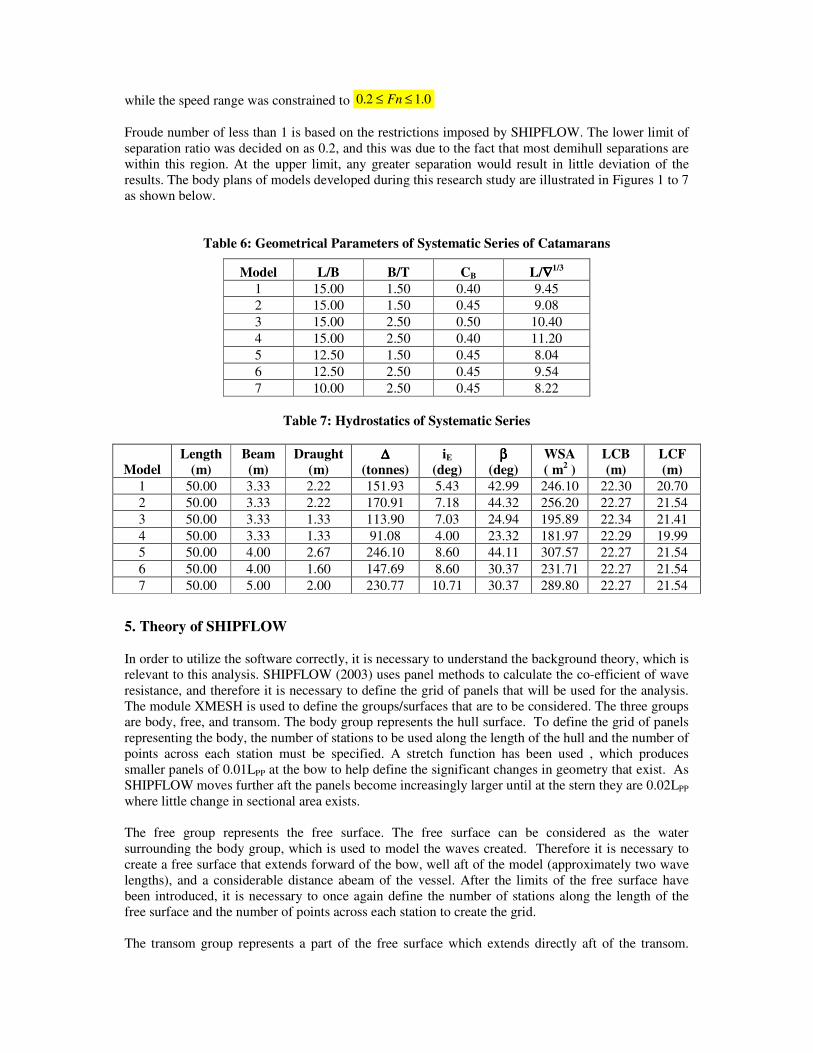
Froude number of less than 1 is based on the restrictions imposed by SHIPFLOW. The lower limit of separation ratio was decided on as 0.2, and this was due to the fact that most demihull separations are within this region. At the upper limit, any greater separation would result in little deviation of the results. The body plans of models developed during this research study are illustrated in Figures 1 to 7 as shown below.

Table 6: Geometrical Parameters of Systematic Series of Catamarans

Model L/B B/T CB L/∇∇∇∇1/3 1 15.00 1.50 0.40 9.45 2 15.00 1.50 0.45 9.08 3 15.00 2.50 0.50 10.40 4 15.00 2.50 0.40 11.20 5 12.50 1.50 0.45 8.04 6 12.50 2.50 0.45 9.54 7 10.00 2.50 0.45 8.22

Table 7: Hydrostatics of Systematic Series

Model Length

(m) Beam (m)

Draught (m)

∆∆∆∆ (tonnes)

iE (deg)

ββββ (deg)

WSA ( m2 )

LCB (m)

LCF (m)

1 50.00 3.33 2.22 151.93 5.43 42.99 246.10 22.30 20.70 2 50.00 3.33 2.22 170.91 7.18 44.32 256.20 22.27 21.54 3 50.00 3.33 1.33 113.90 7.03 24.94 195.89 22.34 21.41 4 50.00 3.33 1.33 91.08 4.00 23.32 181.97 22.29 19.99 5 50.00 4.00 2.67 246.10 8.60 44.11 307.57 22.27 21.54 6 50.00 4.00 1.60 147.69 8.60 30.37 231.71 22.27 21.54 7 50.00 5.00 2.00 230.77 10.71 30.37 289.80 22.27 21.54

5. Theory of SHIPFLOW In order to utilize the software correctly, it is necessary to understand the background theory, which is relevant to this analysis. SHIPFLOW (2003) uses panel methods to calculate the co-efficient of wave resistance, and therefore it is necessary to define the grid of panels that will be used for the analysis. The module XMESH is used to define the groups/surfaces that are to be considered. The three groups are body, free, and transom. The body group represents the hull surface. To define the grid of panels representing the body, the number of stations to be used along the length of the hull and the number of points across each station must be specified. A stretch function has been used , which produces smaller panels of 0.01LPP at the bow to help define the significant changes in geometry that exist. As SHIPFLOW moves further aft the panels become increasingly larger until at the stern they are 0.02LPP where little change in sectional area exists. The free group represents the free surface. The free surface can be considered as the water surrounding the body group, which is used to model the waves created. Therefore it is necessary to create a free surface that extends forward of the bow, well aft of the model (approximately two wave lengths), and a considerable distance abeam of the vessel. After the limits of the free surface have been introduced, it is necessary to once again define the number of stations along the length of the free surface and the number of points across each station to create the grid. The transom group represents a part of the free surface which extends directly aft of the transom.

This group is therefore quite long and only as wide as the vessel. As in the previous section, it is necessary to define the number of stations and points required to produce a grid. For consistency, the number of stations aft of the body must be the same for the free surface as it is for the transom group so that the panels are aligned. The module XPAN is the solver that iteratively converges on the value of co-efficient of wave resistance. It is therefore necessary to input the maximum number of iterations that are to be used. In addition to this, the type of solver that will be used must be specified. The non-linear solver will generally produce a more accurate result than the linear solver, however it is more unstable particularly at high speeds and the solution may not converge. If reference is not made to the type of solver then the linear solver is used as the default. The other important feature of XPAN is whether the model is enabled to freely sink and trim. It is important to note that SHIPFLOW undergoes it analysis by non-dimensionalising the vessel down to a model of unity. Therefore all of the co-ordinates are non-dimensionalised by the length between perpendiculars LPP. As mentioned XMESH module enables the user of SHIPFLOW to construct a grid of panels to illustrate the scenario to be tested. Due to the flexibility of SHIPFLOW to be applied to many different applications, it can produce varying results, which will not match model testing, or full-scale data. The program will produce an accurate result of co-efficient of wave resistance based on the grid supplied, however if the grid is not well set-up the result does not have much validity. One of the major limitations of SHIPFLOW is its inability to model spray and wave-breaking phenomena at high speeds with a Froude number of 1.0 considered as the upper limit. Therefore the investigation has been restricted to this speed. When considering the validity of results there are two key aspects, the precision and the accuracy. If SHIPFLOW is used correctly very precise results may be obtained however these results cannot be considered as accurate until they have been scaled according to some model testing or full-scale data. Therefore, when constructing the grid in SHIPFLOW the aim is to achieve precise results, which can then be altered for accuracy. At low Froude numbers the transom wave has a small wavelength and a large wave height. Conversely, at high Froude numbers the transom wave has a large wavelength with small wave amplitude. Therefore if a constant grid is applied to all of the models at the full range of speeds the degree of precision varies. Therefore caution must be taken when comparing results at different speeds. To overcome this problem, the grid must be systematically altered as the speed is increased to take into account the larger wavelength. This was achieved by increasing the free and transom surfaces further aft until two wavelengths are included as a guideline. On the other hand, at lower speeds it is not necessary to extend the free and transom surfaces further aft of the body group, but it will be necessary to include smaller panels in the grid to account for the significant changes in wave height. If the grid is not altered it can be expected that as the Froude number is increased the results can be considered as becoming increasingly precise. However, as previously mentioned when the speed is increased SHIPFLOW becomes increasingly unstable in its ability to model spray and wave breaking phenomena. Therefore, using this software is a balance of stability and precision and to produce valid results an extensive amount of time is required to analyse the different scenarios. The change in grid density was applied to this analysis to account for changes in Froude numbers. 6. Regression Analysis The type of regression analysis that was performed is called a Forward Stepwise Regression. For this analysis, the wave-resistance co-efficient is the dependent variable. A forward stepwise regression uses one independent variable, and gradually increases the number of variables used in each iteration. The number of iterations is usually the same as the number of cases that are presented for analysis. If an introduced variable is insignificant to the regression analysis it will be discarded.

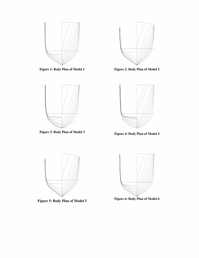
Figure 1: Body Plan of Model 1

Figure 2: Body Plan of Model 2

Figure 3: Body Plan of Model 3

Figure 4: Body Plan of Model 4

Figure 5: Body Plan of Model 5

Figure 6: Body Plan of Model 6

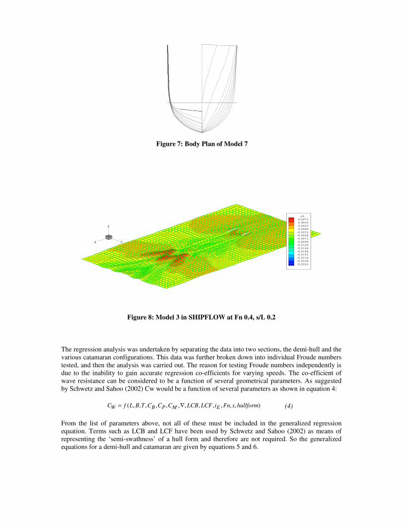
Figure 7: Body Plan of Model 7

X Y

Z

z /L0 . 0 0 7 30 . 0 0 4 90 . 0 0 2 50 . 0 0 0 0

-0 . 0 0 2 4-0 . 0 0 4 8-0 . 0 0 7 2-0 . 0 0 9 6-0 . 0 1 2 0-0 . 0 1 4 4-0 . 0 1 6 8-0 . 0 1 9 2-0 . 0 2 1 6-0 . 0 2 4 0-0 . 0 2 6 4

Figure 8: Model 3 in SHIPFLOW at Fn 0.4, s/L 0.2

The regression analysis was undertaken by separating the data into two sections, the demi-hull and the various catamaran configurations. This data was further broken down into individual Froude numbers tested, and then the analysis was carried out. The reason for testing Froude numbers independently is due to the inability to gain accurate regression co-efficients for varying speeds. The co-efficient of wave resistance can be considered to be a function of several geometrical parameters. As suggested by Schwetz and Sahoo (2002) Cw would be a function of several parameters as shown in equation 4: ),,,,,,,,,,,,( hullformsFniLCFLCBCCCTBLfC EMPBW ∇= (4) From the list of parameters above, not all of these must be included in the generalized regression equation. Terms such as LCB and LCF have been used by Schwetz and Sahoo (2002) as means of representing the ‘semi-swathness’ of a hull form and therefore are not required. So the generalized equations for a demi-hull and catamaran are given by equations 5 and 6.

( ) ( ) ( ) 654

32

13/1

CCE

CC

B

CC

Wdemi iL

CBL

eC ��

����

�

∇���

����

�= (5)

( ) ( ) ( )8

765

432

13/1

CCC

E

CC

B

CCC

Wcat Ls

iL

CTB

BL

eC ���

����

����

����

�

∇���

����

����

����

�= β (6)

X Y

Z

z /L0 . 0 0 8 10 . 0 0 5 60 . 0 0 3 00 . 0 0 0 5

- 0 . 0 0 2 0- 0 . 0 0 4 5- 0 . 0 0 7 1- 0 . 0 0 9 6- 0 . 0 1 2 1- 0 . 0 1 4 6- 0 . 0 1 7 2- 0 . 0 1 9 7- 0 . 0 2 2 2- 0 . 0 2 4 7- 0 . 0 2 7 3

Figure 9: Model 3 in SHIPFLOW at Fn 0.7, s/L 0.2

Equation 6 above was applied to the catamaran regression analyses; however for a demi-hull the (s/L) term becomes insignificant. In addition to this, due to the number of variables compared with the number of cases for a demi-hull analysis, the (B/T) term was not included in the regression (due to the fact that there would be seven models seven independent variables and therefore can not be solved).

Table 8: Regression Coefficients and R2 for demi-hull Configuration

Fn C1 C2 C3 C4 C5 C6 R2 0.2 3.001 -0.159 0.515 -3.666 -0.194 0.000 0.967 0.3 1.221 0.000 0.815 -3.445 0.218 0.000 0.985 0.4 3.180 -0.702 0.377 -3.114 -0.390 0.000 1.000 0.5 2.519 0.396 -0.775 -4.175 0.000 -0.410 0.999 0.6 2.031 -0.239 0.000 -3.402 -0.138 -0.091 0.999 0.7 1.130 -0.220 0.000 -3.221 -0.043 -0.081 0.999 0.8 0.600 -0.272 0.000 -3.079 0.000 -0.063 0.999 0.9 -0.216 0.000 -0.228 -3.158 0.173 -0.178 0.999 1.0 -1.086 0.000 -0.396 -2.965 0.300 -0.203 0.998

In Table 8 the coefficients for the regression analysis have been shown for demi-hull configuration. Also included is the R2 value, which represents the accuracy of the results with 0 providing no correlation and 1 providing complete correlation with the data. As seen above the regression analyses performed are quite good, with the exception being at Fn 0.20. The slightly lower correlation of results is due to the peak is observed on the CW curve, which varies significantly between different models making it harder to model. Also included is the R2 value, which represents the accuracy of the results with 0 providing no correlation and 1 providing complete correlation with the data. As can be seen in figures 10 to 12, the regression analyses performance is quite good for speeds above Fn = 0.5. The slightly lower

correlation of results in the lower speed region is due to the peak observed on the CW curve, which varies significantly between different models making it harder to model. There is generally a very good correlation between results obtained from SHIPFLOW and regression analysis, and therefore the regression analysis can be considered a very good representation of the SHIPFLOW data. The only question to ponder is whether the results obtained from SHIPFLOW are reasonable. Table 9 illustrates the regression coefficients for catamaran configuration.

Table 9: Regression Coefficients and R2 for Catamaran Configuration

Fn C1 C2 C3 C4 C5 C6 C7 C8 R2 0.2 2.571 0.436 0.000 0.000 -4.124 -0.039 -0.199 0.037 0.995 0.3 0.585 0.000 0.000 0.945 -3.282 0.246 0.087 -0.089 0.989 0.4 3.324 0.000 -0.471 -0.963 -3.523 0.000 -0.688 -0.035 0.984 0.5 2.439 0.379 0.000 -0.600 -4.262 0.000 -0.337 -0.368 0.999 0.6 1.809 -0.110 0.000 0.000 -3.625 -0.061 -0.095 -0.314 0.997 0.7 1.055 0.000 0.082 -0.025 -3.617 0.000 -0.064 -0.181 0.997 0.8 0.603 0.222 0.266 0.000 -3.869 0.000 0.000 -0.069 0.998 0.9 -0.466 0.049 0.162 0.000 -3.322 0.128 0.000 -0.006 0.999 1.0 -1.221 0.000 0.117 0.000 -3.046 0.264 0.000 0.075 0.995

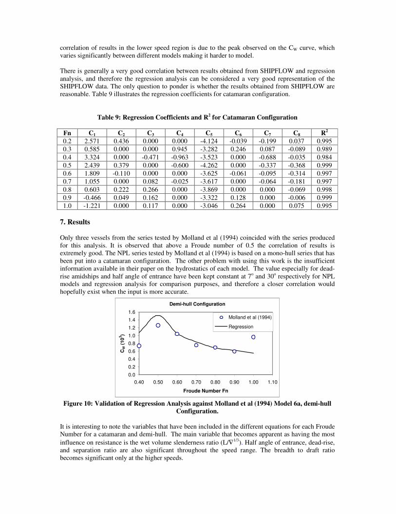
7. Results Only three vessels from the series tested by Molland et al (1994) coincided with the series produced for this analysis. It is observed that above a Froude number of 0.5 the correlation of results is extremely good. The NPL series tested by Molland et al (1994) is based on a mono-hull series that has been put into a catamaran configuration. The other problem with using this work is the insufficient information available in their paper on the hydrostatics of each model. The value especially for dead-rise amidships and half angle of entrance have been kept constant at 7o and 30o respectively for NPL models and regression analysis for comparison purposes, and therefore a closer correlation would hopefully exist when the input is more accurate.

Demi-hull Configuration

0.0

0.2

0.40.6

0.81.0

1.2

1.41.6

0.40 0.50 0.60 0.70 0.80 0.90 1.00 1.10

Froude Number Fn

CW

(103 )

Molland et al (1994)

Regression

Figure 10: Validation of Regression Analysis against Molland et al (1994) Model 6a, demi-hull

Configuration. It is interesting to note the variables that have been included in the different equations for each Froude Number for a catamaran and demi-hull. The main variable that becomes apparent as having the most influence on resistance is the wet volume slenderness ratio (L/∇1/3). Half angle of entrance, dead-rise, and separation ratio are also significant throughout the speed range. The breadth to draft ratio becomes significant only at the higher speeds.

It is interesting to note the variables that have been included in the different equations for each Froude Number for a catamaran and demi-hull. The main variable that becomes apparent as having the most influence on resistance is the slenderness ratio (L/∇1/3). The form factor due to viscous resistance interference factor is another aspect of catamaran resistance that could be further analysed. The work by Armstrong (2000) is limited to the applicable range of low Froude numbers that can be used. Therefore if a similar analysis was undertaken with carefully monitored SHIPFLOW and model testing results, an equation for form factor of catamarans could be produced. This seems to be the least researched aspect of determining catamaran resistance.

Demi-hull Configuration

0.0

0.2

0.4

0.6

0.8

1.0

1.2

1.4

1.6

0.40 0.50 0.60 0.70 0.80 0.90 1.00 1.10

Froude Number Fn

CW

(103 )

Molland et al (1994)

Regression

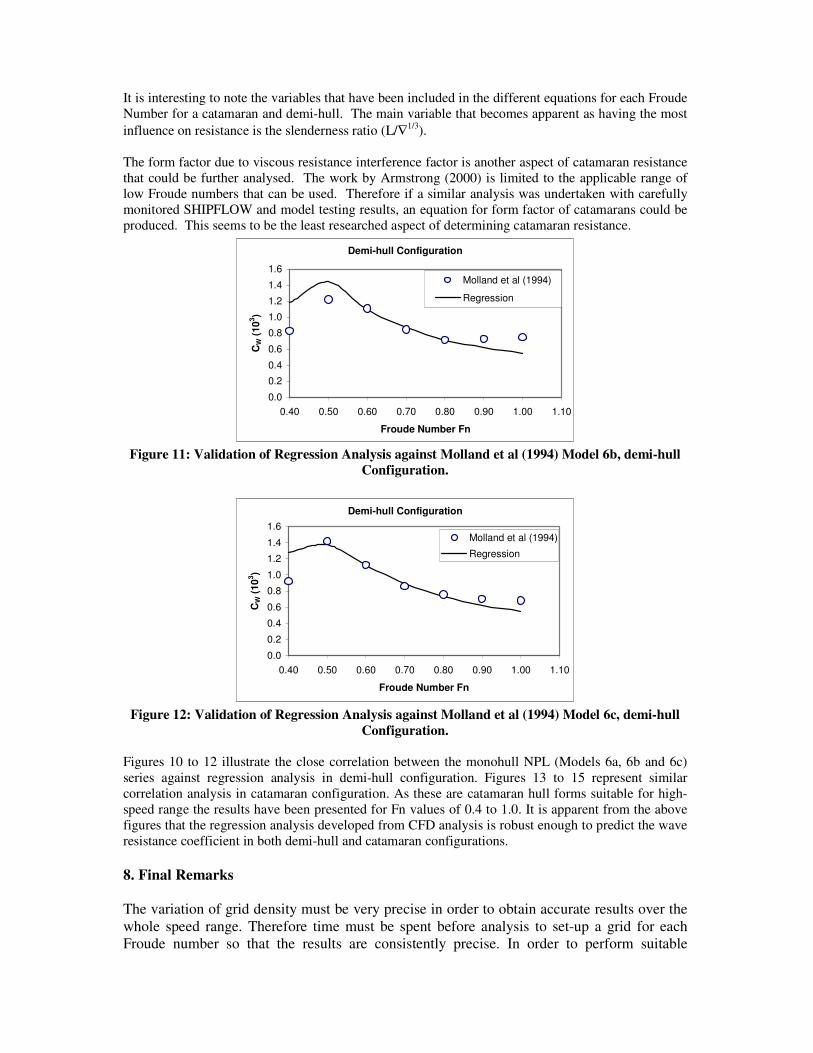
Figure 11: Validation of Regression Analysis against Molland et al (1994) Model 6b, demi-hull

Configuration.

Demi-hull Configuration

0.0

0.2

0.4

0.6

0.8

1.0

1.2

1.4

1.6

0.40 0.50 0.60 0.70 0.80 0.90 1.00 1.10

Froude Number Fn

CW

(103 )

Molland et al (1994)

Regression

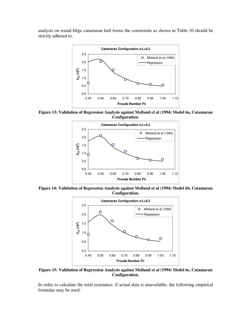
Figure 12: Validation of Regression Analysis against Molland et al (1994) Model 6c, demi-hull

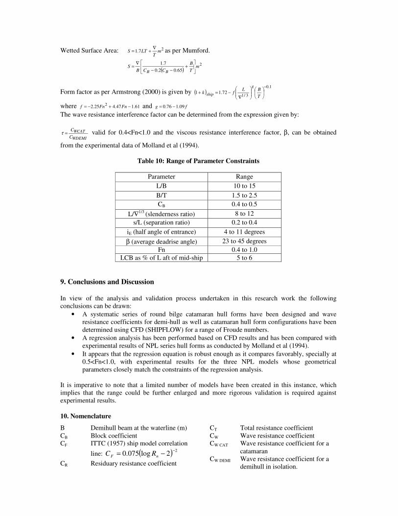
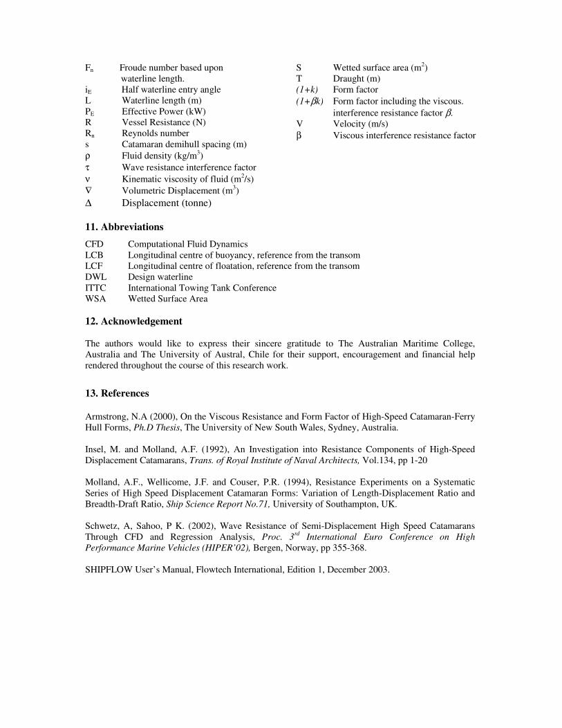
Configuration. Figures 10 to 12 illustrate the close correlation between the monohull NPL (Models 6a, 6b and 6c) series against regression analysis in demi-hull configuration. Figures 13 to 15 represent similar correlation analysis in catamaran configuration. As these are catamaran hull forms suitable for high-speed range the results have been presented for Fn values of 0.4 to 1.0. It is apparent from the above figures that the regression analysis developed from CFD analysis is robust enough to predict the wave resistance coefficient in both demi-hull and catamaran configurations. 8. Final Remarks The variation of grid density must be very precise in order to obtain accurate results over the whole speed range. Therefore time must be spent before analysis to set-up a grid for each Froude number so that the results are consistently precise. In order to perform suitable

analysis on round bilge catamaran hull forms the constraints as shown in Table 10 should be strictly adhered to.

Catamaran Configuration s/L=0.2

0.0

0.5

1.0

1.5

2.0

2.5

0.40 0.50 0.60 0.70 0.80 0.90 1.00 1.10

Froude Number Fn

CW

(103 )

Molland et al (1994)

Regression

Figure 13: Validation of Regression Analysis against Molland et al (1994) Model 6a, Catamaran

Configuration.

Catamaran Configuration s/L=0.2

0.0

0.5

1.0

1.5

2.0

2.5

0.40 0.50 0.60 0.70 0.80 0.90 1.00 1.10

Froude Number Fn

CW

(103 )

Molland et al (1994)

Regression

Figure 14: Validation of Regression Analysis against Molland et al (1994) Model 6b, Catamaran

Configuration.

Catamaran Configuration s/L=0.2

0.0

0.5

1.0

1.5

2.0

2.5

0.40 0.50 0.60 0.70 0.80 0.90 1.00 1.10

Froude Number Fn

CW

(103 )

Molland et al (1994)

Regression

Figure 15: Validation of Regression Analysis against Molland et al (1994) Model 6c, Catamaran

Configuration.

In order to calculate the total resistance, if actual data is unavailable, the following empirical formulae may be used:

Wetted Surface Area: 27.1 mT

LTS∇+= as per Mumford.

( )2

65.02.07.1

mTB

CCBS

BB��

�

�+

−−∇=

Form factor as per Armstrong (2000) is given by ( )1.0

3/172.11

−��

���

����

����

�

∇−=+

TBL

fkg

ship

where 61.147.425.2 2 −+−= FnFnf and fg 09.176.0 −= The wave resistance interference factor can be determined from the expression given by:

WDEMI

WCATCC

=τ valid for 0.4<Fn<1.0 and the viscous resistance interference factor, β, can be obtained

from the experimental data of Molland et al (1994).

Table 10: Range of Parameter Constraints

Parameter Range L/B 10 to 15 B/T 1.5 to 2.5 CB 0.4 to 0.5

L/∇1/3 (slenderness ratio) 8 to 12 s/L (separation ratio) 0.2 to 0.4

iE (half angle of entrance) 4 to 11 degrees β (average deadrise angle) 23 to 45 degrees

Fn 0.4 to 1.0 LCB as % of L aft of mid-ship 5 to 6

9. Conclusions and Discussion In view of the analysis and validation process undertaken in this research work the following conclusions can be drawn:

• A systematic series of round bilge catamaran hull forms have been designed and wave resistance coefficients for demi-hull as well as catamaran hull form configurations have been determined using CFD (SHIPFLOW) for a range of Froude numbers.

• A regression analysis has been performed based on CFD results and has been compared with experimental results of NPL series hull forms as conducted by Molland et al (1994).

• It appears that the regression equation is robust enough as it compares favorably, specially at 0.5<Fn<1.0, with experimental results for the three NPL models whose geometrical parameters closely match the constraints of the regression analysis.

It is imperative to note that a limited number of models have been created in this instance, which implies that the range could be further enlarged and more rigorous validation is required against experimental results. 10. Nomenclature B Demihull beam at the waterline (m) CB Block coefficient CF ITTC (1957) ship model correlation

line: ( ) 22log075.0 −−= nF RC CR Residuary resistance coefficient

CT Total resistance coefficient CW Wave resistance coefficient CW CAT Wave resistance coefficient for a

catamaran CW DEMI Wave resistance coefficient for a

demihull in isolation.

Fn Froude number based upon waterline length. iE Half waterline entry angle L Waterline length (m) PE Effective Power (kW) R Vessel Resistance (N) Rn Reynolds number s Catamaran demihull spacing (m)

S Wetted surface area (m2) T Draught (m) (1+k) Form factor (1+βk) Form factor including the viscous.

interference resistance factor β. V Velocity (m/s) β Viscous interference resistance factor

ρ Fluid density (kg/m3) τ Wave resistance interference factor ν Kinematic viscosity of fluid (m2/s) ∇ Volumetric Displacement (m3) ∆ Displacement (tonne) 11. Abbreviations CFD Computational Fluid Dynamics LCB Longitudinal centre of buoyancy, reference from the transom LCF Longitudinal centre of floatation, reference from the transom DWL Design waterline ITTC International Towing Tank Conference WSA Wetted Surface Area 12. Acknowledgement The authors would like to express their sincere gratitude to The Australian Maritime College, Australia and The University of Austral, Chile for their support, encouragement and financial help rendered throughout the course of this research work.

13. References Armstrong, N.A (2000), On the Viscous Resistance and Form Factor of High-Speed Catamaran-Ferry Hull Forms, Ph.D Thesis, The University of New South Wales, Sydney, Australia. Insel, M. and Molland, A.F. (1992), An Investigation into Resistance Components of High-Speed Displacement Catamarans, Trans. of Royal Institute of Naval Architects, Vol.134, pp 1-20 Molland, A.F., Wellicome, J.F. and Couser, P.R. (1994), Resistance Experiments on a Systematic Series of High Speed Displacement Catamaran Forms: Variation of Length-Displacement Ratio and Breadth-Draft Ratio, Ship Science Report No.71, University of Southampton, UK. Schwetz, A, Sahoo, P K. (2002), Wave Resistance of Semi-Displacement High Speed Catamarans Through CFD and Regression Analysis, Proc. 3rd International Euro Conference on High Performance Marine Vehicles (HIPER’02), Bergen, Norway, pp 355-368. SHIPFLOW User’s Manual, Flowtech International, Edition 1, December 2003.