EXPERIMENT No.1 DETERMINING THE PLATEAU … Manual Radiation... · GEIGER-MULLER COUNTER 1.1 AIM: ... this experiment, you will calculate the efficiency of a GM tube counting system

Department of Nuclear Science and Engineering – SRM University Page 1

EXPERIMENT No.1

DETERMINING THE PLATEAU AND OPTIMAL OPERATING VOLTAGE OF

GEIGER-MULLER COUNTER

1.1 AIM: To determine the plateau and optimal operating voltage of a Geiger-Müller

counter.

1.2 APPARATUS REQUIRED: Geiger-Müller counter, Radioactive Source (e.g., Cs-137,

Sr-90, or Co-60)

1.3 PREPARATION

1.3.1 THEORY

Geiger-Müller (GM) counters were invented by H. Geiger and E.W. Müller in 1928, and

are used to detect radioactive particles. A typical GM Counter consists of a GM tube having a

thin end window (e.g. made of mica), a high voltage supply for the tube, a scalar to record the

number of particles detected by the tube, and a timer which will stop the action of the scalar at

the end of a preset interval.

The sensitivity of the GM tube is such that any particle capable of ionizing a single atom

of the filling gas of the tube will initiate an avalanche of electrons and ions in the tube. The

collection of the charge thus produced results in the formation of a pulse of voltage at the output

of the tube. The amplitude of this pulse, on the order of a volt or so, is sufficient to operate the

scalar circuit with little or no further amplification. The pulse amplitude is largely independent

of the properties of the particle detected, and gives therefore little information as to the nature of

the particle. Even so, the GM Counter is a versatile device which may be used for counting

alpha particles, beta particles, and gamma rays, albeit with varying degrees of efficiency.

Figure 1: Schematic diagram of GM Counter


1.3.2 PRE-LAB QUESTIONS

1. Define Ionization?

2. What are the ionization radiations you know?

3. What is known as GM Region?

4. What is the expression for the voltage developed in a GM counter?

1.4 PROCEDURE

Warning! Dangerous voltages can exist at the GM and SCINT connectors. Ensure that the

high voltage is set to zero or that the instrument is OFF before connecting or disconnecting a

detector.

1. Connect the Power Card of GM counter to its AC adapter.

2. Connect a GM tube to the GM connector via a BNC cable.

3. Enter the HIGH VOLTAGE mode and set the high voltage to the recommended value for the

GM tube.

4. Place the radioactive source close to the GM tube’s window.

5. Using the Operating Mode information described above set the unit up to perform the desired

function.

6. Press the COUNT Button to start data acquisition, the STOP button to halt data acquisition

(providing Preset Time is not being used), and the RESET button to reset the time and data to

zero.

1.5 OBSERVATIONS

1.5.1 FORMULAE / CALCULATIONS

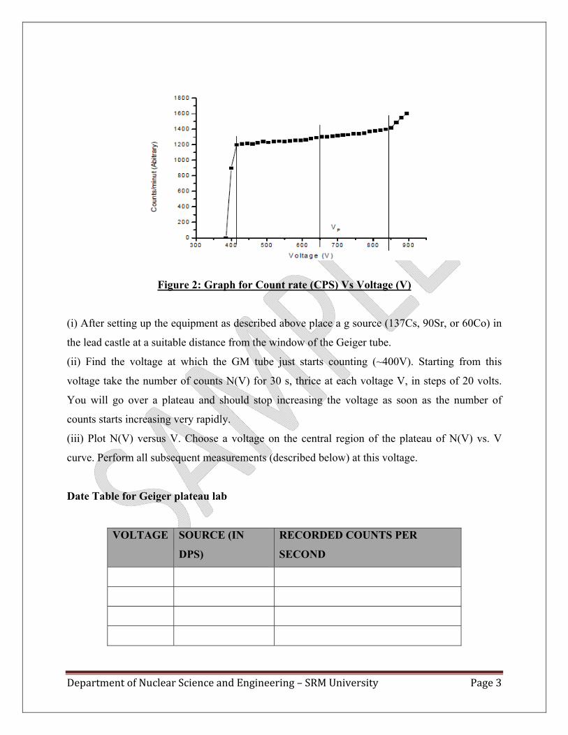
The purpose of this experiment is to determine the voltage plateau for the Geiger tube and to

establish a reasonable operating point for the tube. Fig. 3 shows count rate vs. voltage curve for a

typical Geiger tube that has an operating point in the vicinity of 500 V.


Figure 2: Graph for Count rate (CPS) Vs Voltage (V)

(i) After setting up the equipment as described above place a g source (137Cs, 90Sr, or 60Co) in

the lead castle at a suitable distance from the window of the Geiger tube.

(ii) Find the voltage at which the GM tube just starts counting (~400V). Starting from this

voltage take the number of counts N(V) for 30 s, thrice at each voltage V, in steps of 20 volts.

You will go over a plateau and should stop increasing the voltage as soon as the number of

counts starts increasing very rapidly.

(iii) Plot N(V) versus V. Choose a voltage on the central region of the plateau of N(V) vs. V

curve. Perform all subsequent measurements (described below) at this voltage.

Date Table for Geiger plateau lab

VOLTAGE SOURCE (IN

DPS)

RECORDED COUNTS PER

SECOND


Graph: Counts Per Seconds Vs Voltage given.

1.6 POST-LAB QUESTIONS

1. How do you find optimal Voltage for a Geiger – Muller counter?

2. What is DPS means?

3. How you can get maximum efficiency from a Geiger – Muller counter

1.7 INFERENCES

1.8 RESULT

The Optimal Voltage of the given Geiger – Muller Counter is = ------ Volts

Counts Per Seconds Vs Voltage given graph has been drawn to identify the plateau

region of the GM counter.


EXPERIMENT No.2

DETERMINING THE EFFICIENCY OF A GEIGER-MULLER COUNTER

1.1 AIM: To determining the Efficiency of a Geiger-Muller counter


Sr-90, or Co-60)

1.3 PREPARATION

1.3.1 THEORY

From earlier experiments, you should have learned that a GM tube does not count all the

particles, which are emitted from a source (like, dead time). In addition, some of the particles do

not strike the tube at all, because they are emitted uniformly in all directions from the source. In

this experiment, you will calculate the efficiency of a GM tube counting system for different

isotopes by comparing the measured count rate to the disintegration rate (activity) of the source.

To find the disintegration rate, change from microCuries (µCi) to disintegrations per minute

(dpm). The disintegrations per minute unit is equivalent to the counts per minute from the GM

tube, because each disintegration represents a particle emitted.

The conversion factor is:

1 Ci = 2.22 x 1012 dpm or 1 µCi = 2.22 x 106 dpm (1)

Multiply this by the activity of the source and you have the expected counts per minute of the

source. We will use this procedure to find the efficiency of the GM tube, by using a fairly simple

formula. You want to find the percent of the counts you observe versus the counts you expect, so

you can express this as

% Efficiency = r(100)/CK (2)

In this formula, r is the measured activity in cpm, C is the expected activity of the source in µCi,

and K is the conversion factor


1. What is the Expression to find out the Efficiency of a Counter?

2. Define Radioactivity and its units?

3. How you can convert Curie in to Bq?


1.4 PROCEDURE



detector.




GM tube. (You can use the previous experiment result)



function.



zero.

1.5 OBSERVATIONS


1. Setup the Geiger counter as you have in the previous experiments. Set the Voltage of the

GM tube to its optimal operating voltage, which should be around 900 Volts.

2. Set Runs to zero and set Preset Time to 60 to measure activity in cpm.

3. First do a run without a radioactive source to determine your background level.

4. Next, place one of the radioactive sources (Po-210, Sr-90, Co-60) in the top shelf and

begin taking data.

5. Repeat this for each of your other two sources. Remember that the first run is a

background number.

6. (OPTIONAL) From the Preset menu, change the Preset Time to 300, and take data for all

three sources again.

7. Save your data to disk or to a data table before exiting the ST350 program.


Table

Run Duration = …. Seconds Background counts:

SOURCE COUNTS CORRECTION

IN COUNTS

EXPECTED

COUNTS

EFFICIENCY


1. What is Efficiency of an ordinary GM Counter?

2. What are Efficiency affecting factors?

1.7 INFERENCES

1.8 RESULT

The Efficiency of a GM counter is = ------ (%)


EXPERIMENT No.3

DETERMINING THE RESOLVING (DEAD) TIME τ OF A GEIGER – MULLER

COUNTER

1.1 AIM: To determining the resolving (dead) time τ of a Geiger – Muller counter.


Sr-90, or Co-60)

1.3 PREPARATION

1.3.1 THEORY

A Geiger-Mueller (G-M) tube dead time is the time interval after the initiation of a

normal-size pulse during which the tube is insensitive to further ionization events. The resolving

(or resolution) time of a G-M tube, or when combined with a counting system, is the minimum

time interval between two distinct ionizing events, which permit both to be counted.

The ideal GM tube should produce a single pulse on entry of a single ionising particle. It

must not give any spurious pulses, and must recover quickly to the passive state. Unfortunately

for these requirements, when positive argon ions reach the cathode and become neutral argon

atoms again by obtaining electrons from it, the atoms can acquire their electrons in enhanced

energy levels. These atoms then return to their ground state by emitting photons which can in

turn produce further ionisation and hence cause spurious secondary pulse discharges. If nothing

were done to counteract it, ionisation could even escalate, causing a so-called current

"avalanche" which if prolonged could damage the tube. Some form of quenching of the

ionisation is therefore essential. The disadvantage of quenching is that for a short time after a

discharge pulse has occurred (the so-called dead time, which is typically 50 - 100 microseconds),

the tube is rendered insensitive and is thus temporarily unable to detect the arrival of any new

ionising particle. This effectively causes a loss of counts at sufficiently-high count rates and

limits the G-M tube to a count rate of between 104 to 105 counts, depending on its characteristic


1. What is a Dead Time of Counter?

2. Which counter is more sensitive ionization chamber or GM Counter?

3. What is the Expression for finding the dead time of a counter?


1.4 PROCEDURE



detector.




GM tube. (You can use the Previous experiment result)



function.



zero.

1.5 OBSERVATIONS


A commonly used method for dead time measurements is known as two source method. The

method is based on observing the counting rate from two sources individually and in

combination. Because the counting losses are nonlinear, the observed rate due to the combined

sources will be less than the sum of the rates due to the two sources counted individually, and the

dead time can be calculated from the discrepancy.

(i) To find the dead time we have to use two γ sources say S1 (137Cs) and S2 (60Co). While

performing the experiment as per the steps given below, care must be exercised not to move the

source already in place and consideration must be given to the possibility that the presence of a

second source will scatter radiation into the detector which would not ordinarily be counted from

the first source alone. In order to keep the scattering unchanged, a dummy second source without

activity is normally put in place when the sources are counted individually.

(ii) Keep source S1 in one of the pits in the source holder made for this purpose. Keep a dummy

source in the second pit. Record the counts for a preset time (say 300 s).


(iii) Without removing source S1 remove the dummy source from the second pit and keep the

source S2 in its place. Record the number of counts for the combined sources S1 and S2 for the

same preset time as in (ii).

(iv) Remove source S1 and measure the counts due to source S2 alone, for the same preset time

as in (ii).

(v) Remove source S2 as well and record the background counts for the same period.

Calculate the count rates in all the cases. Let n1, n2 and n12 be the true counts (sample plus

background), with sources S1, S2 and (S1 +S2), respectively. Let m1, m2 and m12 represent the

corresponding observed rates. Also let nb and mb be the true and measured background rates

with both the sources removed. Assuming the nonparalyzable model, the dead time �is given by

YZX )1( −

=τ ---- (1)

Where X= m1m2 - mbm12

Y=m1m2 (m12+mb) - mbm12 (m1+m2)

Z = Y(m1+m2-m12-mb )/ X2

Table

Run duration = …. Seconds Back ground = -----Counts

Source n m τ Error (%)

S1

S2

S3


1. What is your GM tube’s resolving (or dead) time? Does it fall within the accepted 1 �s to

100 �s range?

2. Is the percent of correction the same for all your values? Should it be? Why or why not?

1.7 INFERENCES


1.8 RESULT

The Dead time of the GM counter is = ------ Seconds


EXPERIMENT No.4

DETERMINING THE HALF LIFE OF A RADIO ISOTOPE USING GEIGER –

MULLER COUNTER

1.1 AIM: To determining the half life of a radio isotope.


Sr-90, or Co-60)

1.3 PREPARATION

1.3.1 THEORY

The decay of radioactive atoms occurs at a constant rate. There is no way to slow it down. The

rate of decay is also a constant fixed rate regardless of the amount of radioactive atoms present.

That is because there are only two choices for each atom, decay or don’t decay. Thus, the amount

of radioactive atoms we have on hand at any time is undergoing a consistent, continuous change.

The change in the number of radioactive atoms is a very orderly process. If we know the number

of atoms present and their decay constant (probability of decay per unit time), then we can

calculate how many atoms will remain at any future time. This can be written as the equation

N(t) = N - λN∆t , (1)

where N(t) is the number of atoms that will be present at time t, N is the number of atoms present

currently, λis the decay constant, and ∆t is the elapsed time. If the number of radioactive atoms

remaining is plotted against time, curves like those in Figure can be obtained. The decay

constant can be obtained from the slope of these curves (discussed more below).


A more common way of expressing the decay of radioactive atoms is the half-life. The half-life

of a radioactive isotope is the time required for the disintegration of one-half of the atoms in the

original sample. In the graphs in Figure 8, 1000 atoms were present at t = 0. At the end of one

half-life, 500 atoms were present. At the end of two half lives, 250 atoms were present, one

quarter of the original sample. since activity (Each count of a

GM tube represents one atom decaying and releasing one particle or ray of radiation.)

we can solve for the half-time


1. What is radioactivity?

2. What is a half life of a radio isotope?

3. Which the expression for a decay constant in terms of half life?

1.4 PROCEDURE



detector.





GM tube. (You can use the Previous experiment result)



function.



zero.

1.5 OBSERVATIONS


1. Setup the Geiger counter as you have in the previous experiments. Set the Voltage of the GM

tube to its optimal operating voltage, which should be around 900 Volts.

2. From the Preset menu, set Runs to zero and set Preset Time to 30.

3. First do a run without a radioactive source to determine your background level.

4. Next, from the Preset menu, set the Runs to 31. (This will take 30 more runs so the total

Number of runs is 31.)

5. Place the radioactive source in the second shelf from the top and begin taking data.

6. Record the data to a file on disk or into a data table.

7. You may wish to do a second trial if time allows.

Table

Run duration = …. Seconds Back ground = -----Counts

TIME COUNTS CORRECTED

COUNTS

In (COUNTS)

30

60

90

120

…

690

720


Table :

DATE τ λ ERROR COUNTING

STATISTICS


1. Is the half life of a radio isotope is changing time to time?

2. What are all the type of errors occurred in during the experiment

Precautions:

1. While performing an experiment with one radioactive source other sources should not be

present nearby. They should be put behind the lead shield.

2. Handle the radioactive sources with care. Don’t touch in bare hand to the center of

samples.

3. While handling the liquid radioactive samples please use hand gloves.

4. Don’t put your mobile near to the detector. It may add some counts to the signal.

1.7 INFERENCES

1.8 RESULT

The half life of the given radio isotope is = ------ Seconds


EXPERIMENT No.5

DETERMINING THE EFFICIENCY OF A ENVIRONMENTAL SURVEY METER

1.1 AIM: To determining the Efficiency of a Environmental Survey Meter

1.2 APPARATUS REQUIRED: Environmental Survey Meter, Radioactive Source (e.g.,

Cs-137, Sr-90, or Co-60)

1.3 PREPARATION

1.3.1 THEORY

Portable Radiation Survey Monitor Model PRSM-2 is a micro-controller based, portable

battery operated instrument for measurement of environmental/ field dose rate of Gamma and X-

ray radiations. It is useful for Health Physics applications in Radioisotope Laboratories, Nuclear

Power Plants and nuclear medical centres. Environmental Survey Meter employs either an

internal or external GM detector for direct readout of either dose rate or counts for selected time

interval. It is powered by 4 nos of Ni-MH type rechargeable batteries. And it is equipped with

Audio Chirper and can be turned ON / OFF as per users choice. 64 X 128 pixel Graphic Display

provides interactive Menu and Dose Rate Display / Counts

To find the disintegration rate, change from microCuries (µCi) to disintegrations per

minute (dpm). The disintegrations per minute unit is equivalent to the counts per minute from the

ERS, because each disintegration represents a particle emitted.


1 Ci = 2.22 x 1012 dpm or 1 µCi = 2.22 x106 dpm (1)


source. We will use this procedure to find the efficiency of the ESM, by using a fairly simple




In this formula, r is the measured activity in cpm, C is the expected activity of the source in

µCi,and K is the conversion factor



1. What is the penetration ability of alpha, beta and gamma radiations?

2. What is a principle GM Counter?

1.4 PROCEDURE



detector.

1. Switch on the ERS (PRSM-1).

2. Check the battery level in the indictor.

3. Set the Run mode in to CPS

4. Place the radioactive source close to the ERS.

5. Using the integration time to either 1/5/10seconds.


1.5 OBSERVATIONS


Table

Run Duration = -----Seconds Background counts:


IN COUNTS

EXPECTED

COUNTS

EFFICIENCY


1. What is Efficiency of an ordinary GM Counter and ERS?

2. How you can calibrate the ERS after knowing its Efficiency?

1.7 INFERENCES

1.8 RESULT

The Efficiency of a ERS is = ------ (%)


EXPERIMENT No.6

DETERMINING THE EFFICIENCY OF A GIVEN ALPHA SOURCE

1.1 AIM: To determining the efficiency of a given unknown alpha emitting radio isotoper

1.2 APPARATUS REQUIRED: alpha counter, Radioactive Source (e.g., Am-241 )

1.3 PREPARATION

1.3.1 THEORY

Alpha detector (PNC-Alpha) is a micro controller based scintillation detector uses ZnS(Ag)

Scintillator as it is detector, which is protected by a MYLAR sheet. A scintillation detector or

scintillation counter is obtained when a Scintillator is coupled to an electronic light sensor such

as a photomultiplier tube (PMT) or a photodiode. PMTs absorb the light emitted by the

scintillator and reemit it in the form of electrons via the photoelectric effect. The subsequent

multiplication of those electrons (sometimes called photo-electrons) results in an electrical pulse

which can then be analyzed and yield meaningful information about the particle that originally

struck the scintillator.

To find the disintegration rate, change from microCuries (µCi) to disintegrations per

minute (dpm). The disintegrations per minute unit is equivalent to the counts per minute from the

ERS, because each disintegration represents a particle emitted.


1 Ci = 2.22 x 1012 dpm or 1µCi = 2.22x 106 dpm (1)


source. We will use this procedure to find the efficiency of the ESM, by using a fairly simple




In this formula, r is the measured activity in cpm, C is the expected activity of the source in

µCi,and K is the conversion factor



1. What is the principle of a Scintillation detector?

2. Define Luminescence

3. How a Photo Multiplier Tube is working?

1.4 PROCEDURE



detector.

1. Make connections to Radiation Counting System with alpha probe.

2. Power up the Radiation Counting System unit & increase the HV to Alpha probe to operating

voltage.

3. For a known preset time (say)100 seconds take background (BG) counts.

4. Now place standard Alpha source of known DPS & count for same time

5. By subtracting the BG obtain net counts (CPM)

6. Take ratio of CPM Vs DPM to obtain efficiency of the probe.

1.5 OBSERVATIONS


Table

Run Duration = -----Seconds Background counts:


IN COUNTS

EXPECTED

COUNTS

EFFICIENCY

1.6 INFERENCES

1.7 RESULT

The Efficiency of an alpha counter is = ------ (%)


EXPERIMENT No.7

DETERMINING THE PROPERTIES OF NAI DETECTOR

1.1 AIM: To determining the properties of NaI detector

1.2 APPARATUS REQUIRED: NaI based gamma ray spectrometer, Radioactive Source

(e.g., Cs-137, Co-60 )

1.3 PREPARATION

1.3.1 THEORY

Gamma ray spectroscopy is one of the most developed and important techniques used in

experimental nuclear physics because gamma ray detection and its energy measurement form an

essential part of experimental nuclear physics research. The purpose of this experiment is to

acquaint one with this field using a gamma ray spectrometer comprising of thallium activated

sodium iodide (NaI(Tl)) scintillator, photo multiplier tube, associated electronics and multi

channel analyzer. The scintillation spectrometers with their high detection efficiency and

moderately good energy resolution have made tremendous contribution to our present knowledge

of nuclear properties.

The detection of gamma rays occurs through its interaction with the detecting medium,

(NaI (Tl) in the present case). There are three important processes by which gamma ray photons

interact with matter enabling us to detect them and measure their energies. These processes are

the following.

(i) Photoelectric Absorption

Photoelectric absorption is an interaction in which the incident gamma ray photon

disappears. In its place, a photoelectron is released from one of the electron shells of the absorber

atom with a kinetic energy given by the incident photon energy h minus the binding energy of

the electron in its original shell (EB). The interaction is with the atom as a whole and cannot take

place with free electrons. For typical gamma ray energies, the photoelectron is most likely to

emerge from the K shell of the atoms for which typical binding energies range from a few keV

for low-Z materials to tens of keV for materials with higher atomic number. After the ejection of

an electron by this process, the vacancy in that shell of the atom is filled up by another electron

from outer shells. This is followed by emission of X-rays or Auger electrons consuming the

binding energy EB. The configuration of the atomic shells recovers within a very short time after

the photoelectric emission. The atomic X-rays produced as a follow-up of the photoelectric effect


are almost completely absorbed by the matter surrounding the point of emission, giving rise to

further photoelectrons. Thus the total energy of the incident gamma ray is completely converted

into the kinetic energy of the electrons and thus one gets an output which is proportional to the

energy of ejected electrons. (Here the energy of the ejected electrons (E-28) KeV, E = h is the

energy of the incident gamma ray and 28 KeV is the binding energy of K shell of an electron in

the iodine atom). Therefore in general, one expects two peaks in photoelectric absorption

corresponding to E and (E-28) KeV but they are not often resolved due to limit on resolution.

(ii) Compton Effect

a. Compton Scattering

In this process an incident photon interacts with a free electron, gets scattered and leaves

the detector. Compton scattering also includes scattering of the photon by electrons bound to an

atom because in comparison to the energy of the photon, the electron binding energy is quite

small. Thus an incident photon of energy h can be considered to collide with a free electron of

rest mass m0. The photon is scattered through an angle with an energy h/(<h) while the electron

recoils with a kinetic energy K e at an angle .

b. Back Scattering

Back scattering peak derives its origin from the detection of gamma rays scattered by the

material of which the source is made. These gamma rays are scattered at 180o , then enter the

crystal and absorbed by photoelectron emission and thus have energy, E/(1+2 ) as explained

before. In this particular detector E=0.5 MeV and 2 MeV and we expect back scattering peaks at

0.17 and 0.22 MeV, respectively.

(iii) Pair Production

When a photon having energy greater than 1.02 MeV strikes a material of high atomic

number, it is found that it is completely absorbed and a pair of electron and positron is produced.

This process is known as pair production and the cutoff energy of the photon is 1.02 MeV. The

conservation of energy yields hv=2m0c2 + E+ + E- + Enuclear, where 2m0c2 is the rest mass energy

of the pair while E+, E- and E(nuclear) are the kinetic energies of the positron, electron and

nucleus, respectively. The presence of the nucleus is essential for the conservation of linear

momentum.

The kinetic energy of the pair is then (E-1.02) MeV (where E=h) which is shared equally

between the electron and the positron which are stopped in the crystal. The positron annihilates


with the nearest electron available and produces two oppositely directed gamma rays of total

energy 1.02 MeV. Both or one of these annihilation gamma rays (each having energy of m0c2=

511 KeV) can either be stopped in the crystal through processes photoelectric absorption and

Compton or they can escape from the crystal. In case both the photons are completely stopped in

the crystal one will get a full energy peak at E, as in the case of photoelectric absorption. If one

or both gamma rays escape we get a corresponding peak at energies E - m0c2 or E - 2m0c2.

As an example of one extreme in gamma ray detector behavior, we first examine the

expected response of detectors whose size is small compared with the mean free path of the

secondary gamma radiations produced in interactions of the original gamma rays. These

secondary radiations are Compton scattered gammas, together with annihilation photons formed

at the end of the tracks of positrons created in pair productions. Because the mean free path of

the secondary gamma rays is typically of the order of several centimeters, the condition of

“smallness” is met if the detector dimensions do not exceed a centimeter or two. At the same

time, we assume that all charged particle energies (photoelectron, Compton electron, and

positron) are completely absorbed within the detector volume.

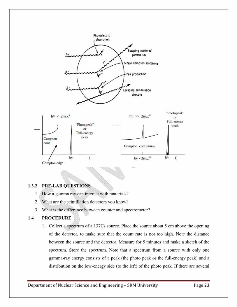
The predicted electron energy deposition spectra under these conditions are illustrated in

Fig.1. If the incident gamma ray energy is below the value at which pair production is possible,

the spectrum results only from the combined effect of Compton scattering and photoelectric

absorption. The continuum of energies corresponding to Compton scattered electrons is called

the Compton continuum, whereas the narrow peak corresponding to photoelectrons is designated

as photopeak. For a small detector only single interactions take place, and the ratio of the area

under the photopeak to the area under the Compton continuum is the same as the ratio of the

photoelectric cross section to the Compton cross section in the detector material.

If the incident gamma ray energy is sufficiently high (several MeV), the results of pair

production are also evident in the electron energy spectrum. For a small detector, only the

electron and positron kinetic energies are deposited, and the annihilation radiation escapes. The

net effect is to add a double escape peak to the spectrum located at an energy 2m0c2 (~1.02 meV)

below the photopeak. The term double refers to the fact that the annihilation photons escapes.



1. How a gamma ray can interact with materials?

2. What are the scintillation detectors you know?

3. What is the difference between counter and spectrometer?

1.4 PROCEDURE

1. Collect a spectrum of a 137Cs source. Place the source about 5 cm above the opening

of the detector, to make sure that the count rate is not too high. Note the distance

between the source and the detector. Measure for 5 minutes and make a sketch of the

spectrum. Store the spectrum. Note that a spectrum from a source with only one

gamma-ray energy consists of a peak (the photo peak or the full-energy peak) and a

distribution on the low-energy side (to the left) of the photo peak. If there are several


photo peaks in a spectrum, the studied radiation must contain several different

energies.

2. The low-energy distribution to the left of the photo peak originates from gamma

quanta, which have collided with electrons in the detector crystal or in the lead

shielding. The collision takes place in such a way that only part of the original energy

of the gamma quantum is absorbed in the detector. This kind of collision is called

Compton scattering and the low-energy distribution is the so-called Compton

distribution. The Compton distribution always forms a background to the left of the

photo peak with which it is associated.

3. Note that there is always a discriminator setting, which rejects the most low-energetic

gamma quanta and the electronic noise. The discriminator setting can be adjusted

with the knob on the amplifier box, but should not be changed during a measurement.

4. Note in your sketch of the 137Cs spectrum where the photo peak, discriminator level

and Compton distribution are situated.

5. Record a spectrum of KCl or of the mineral salt. The mineral salt contains KCl, and

thus 40K, which is a naturally occurring radioactive isotope. Measure for 15 minutes

and then make a sketch of the spectrum. Compare with the background spectrum.

Save the spectrum.

6. Record a background spectrum, i.e. collect a spectrum without a source. The

measuring time is 20 minutes. Don't forget to remove all sources close to the detector.

Save the background spectrum. Compare with the 40K spectrum in b.

Precautions:

1. While performing an experiment with one radioactive source other sources should not

be present nearby. They should be put behind the lead shield.

2. Handle the radioactive sources with care. Don�t touch in bare hand to the center of

samples.


4. Don�t put your mobile near to the detector. It may add some counts to the signal.

5. Amplifier and detector are always running at high voltage. So please don�t switch

off any part during the data acquisition, it may damage the amplifier and detector.


1.5 OBSERVATIONS

Example Spectrum:

Table: For a 137Cs spectrum

ITEM ENERGY (MeV) CHANNEL NO

Photo Peak 0.662

Compton Edge 1.17

Back Scatterd Peak 1.33

Area under the Photo Peak

1.6 INFERENCES

1.7 RESULT

The Photo Peak for the 137Cs is found in the Energy = ------ (MeV)


EXPERIMENT No.8

ENERGY CALIBRATION OF NAI DETECTOR WITH 137-CS AND 60-CO

1.1 AIM: To calibrate the NaI detector using 137Cs and 60Co sources

1.2 APPARATUS REQUIRED: NaI based gamma ray spectrometer, Radioactive Source

(e.g., Cs-137, Co-60 )

1.3 PREPARATION

1.3.1 THEORY

NaI detector consists of a single crystal of thallium activated sodium iodide optically coupled to

the photocathode of a photomultiplier tube. When a gamma ray enters the detector, it interacts by

causing ionization of the sodium iodide. This creates excited states in the crystal that decay by

emitting visible light photons. This emission is called a scintillation, which is why this type of

sensor is known as a scintillation detector. The thallium doping of the crystal is critical for

shifting the wavelength of the light photons into the sensitive range of the photocathode.

Fortunately, the number of visible-light photons is proportional to the energy deposited in the

crystal by the gamma ray. After the onset of the flash of light, the intensity of the scintillation

decays approximately exponentially in time, with a decay time constant of 250 ns. Surrounding

the scintillation crystal is a thin aluminum enclosure, with a glass window at the interface with

the photocathode, to provide a hermetic seal that protects the hygroscopic NaI against moisture

absorption. The inside of the aluminum is lined with a coating that reflects light to improve the

fraction of the light that reaches the photocathode. At the photocathode, the scintillation photons

release electrons via the photoelectric effect. The number of photoelectrons produced is

proportional to the number of scintillation photons, which, in turn, is proportional to the energy

deposited in the crystal by the gamma ray. The remainder of the photomultiplier tube consists of

a series of dynodes enclosed in the evacuated glass tube. Each dynode is biased to a higher

voltage than the preceding dynode by a high voltage supply and resistive biasing ladder in the

photomultiplier tube base. Because the first dynode is biased at a considerably more positive

voltage than the photocathode, the photoelectrons are accelerated to the first dynode. As each

electron strikes the first dynode the electron has acquired sufficient kinetic energy to knock

out 2 to 5 secondary electrons. Thus, the dynode multiplies the number of electrons in the pulse

of charge. The secondary electrons from each dynode are attracted to the next dynode by the

more positive voltage on the next d ynode. This multiplication process isrepeated at each dynode,


until the output of the last dynode is collected at the anode. By the time the avalanche of charge

arrives at the anode, the number of electrons has been multiplied by a factor ranging from 104 to

106, with higher applied voltages yielding larger multiplication factors. For the selected bias

voltage, the charge arriving at the anode is proportional to the energy deposited by the gamma

ray in the scintillator. The preamplifier collects the charge from the anode on a capacitor, turning

the charge into a voltage pulse. Subsequently, it transmits the voltage pulse over the long

distance to the supporting amplifier. At the output of the preamplifier and at the output of the

linear amplifier, the pulse height is proportional to the energy deposited in the scintillator by the

detected gamma ray. The Multichannel Analyzer (MCA) measures the pulse heights delivered by

the amplifier, and sorts them into a histogram to record the energy spectrum produced by the

NaI(Tl) detector. See Figure 1 for the modular electronics used with the NaI(Tl) detector. For an

ideal detector and supporting pulse processing electronics, the spectrum of 662-keV gamma rays

from a 137Cs radioactive source would exhibit a peak in the spectrum whose width is

determined only by the natural variation in the gamma-ray energy. The NaI(Tl) detector is far

from ideal, and the width of the peak it generates is typically 7% to 10% of the 662-keV gamma-

ray energy. The major source of this peak broadening is the number of photoelectrons emitted

from the photocathode for a 662-keV gamma-ray. For a high-quality detector this is on the order

of 1,000 photoelectrons. Applying Poisson statistics 1,000 photoelectrons limit the full width of

the peak at half its maximum height (FWHM) to no less than 7.4%. Statistical fluctuations in the

secondary electron yield at the first dynode and fluctuations in the light collected from the

scintillator also make a small contribution to broadening the width of the peak in the energy

spectrum. Because the broadening is dominated by the number of photoelectrons, and that

number is proportional to the gamma-ray energy, the FWHM of a peak at energy E is

approximately described by

Where

E is the energy of the peak,

δE is the FWHM of the peak in energy units, and

k is a proportionality constant characteristic of the particular detector.



1. How a gamma ray can interact with materials?

2. What are the scintillation detectors you know?

3. What is the difference between counter and spectrometer?

1.4 PROCEDURE

Return the 137Cs source to the counting position, and implement an acquisition for a time period

long enough to form a well defined spectrum with minimal random scatter in the vertical

direction. The amount of scatter is controlled by counting statistics. If the ith channel contains Ni

counts, the standard deviation in those counts is expected to be And the percent standard

deviation in the Ni counts is Note that 100 counts in a channel corresponds to a 10% standard

deviation, 10,000 c ounts yield a 1% standard deviation, and 1 million counts are needed to

achieve a 0.1% standard deviation. Consequently, the vertical scatter in the spectrum will begin

to appear acceptable when the rather flat continuum at energies below the Compton edge has

more than a few hundred counts per channel.

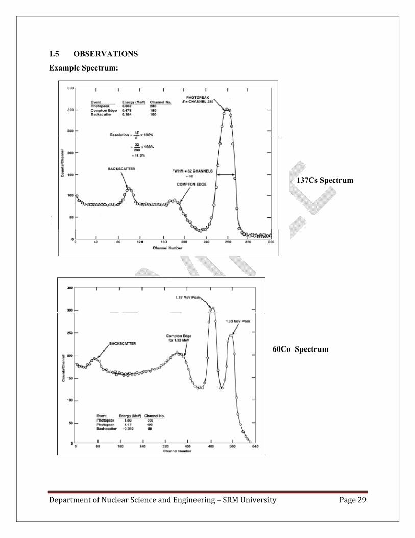
2. Plot the spectrum accumulated in step 1 with a linear vertical scale. Mark the photopeak, the

Compton edge and the backscatter peak (if discernable) on the spectrum as indicated in Figure

3. Determine the channel number for the 662-keV peak position.

4. After the 137Cs spectrum has been read from the MCA, save it in a file that you designate for

possible later recall. Erase the spectrum, and replace the 137Cs source with a 60Co source from

the gamma source kit.

5. Accumulate the 60Co spectrum for a period of time long enough for the spectrum

6. Save the 60Co spectrum for possible later recall and plot the spectrum.

Precautions:

1. While performing an experiment with one radioactive source other sources should not

be present nearby. They should be put behind the lead shield.

2. Handle the radioactive sources with care. Don�t touch in bare hand to the center of

samples.


4. Don�t put your mobile near to the detector. It may add some counts to the signal.

5. Amplifier and detector are always running at high voltage. So please don�t switch

off any part during the data acquisition, it may damage the amplifier and detector.


1.5 OBSERVATIONS

Example Spectrum:

137Cs Spectrum

60Co Spectrum


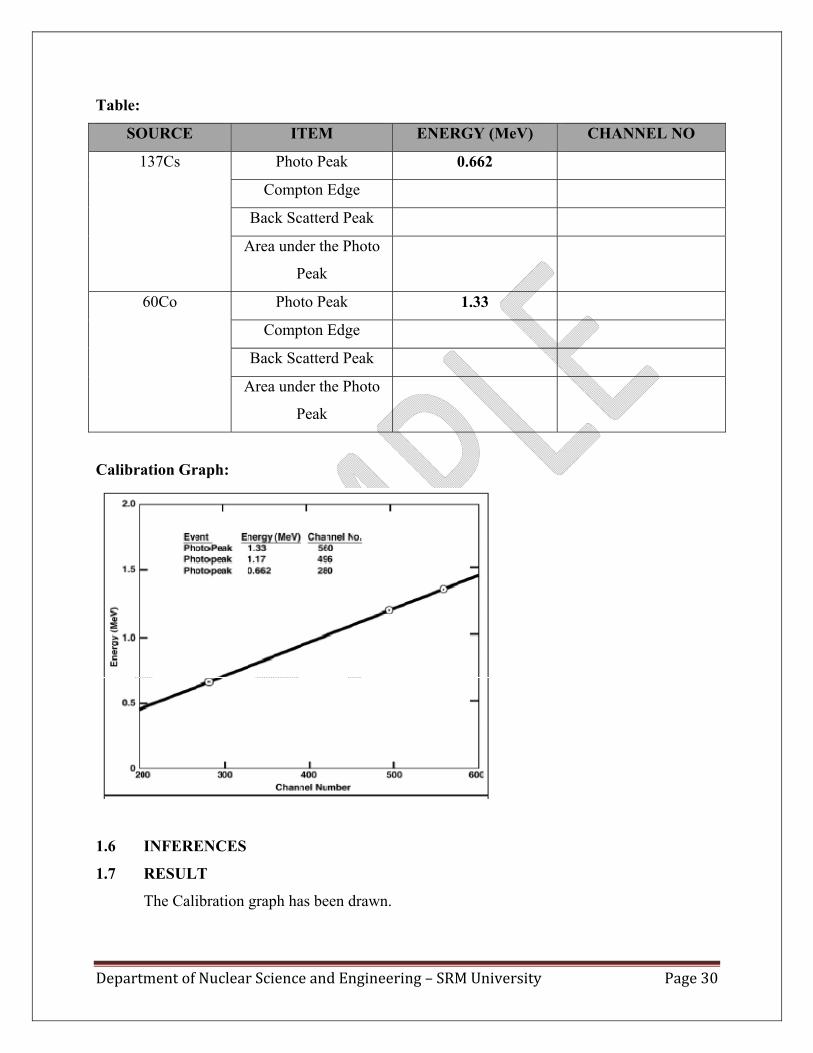
Table:

SOURCE ITEM ENERGY (MeV) CHANNEL NO

137Cs Photo Peak 0.662

Compton Edge

Back Scatterd Peak

Area under the Photo

Peak

60Co Photo Peak 1.33

Compton Edge

Back Scatterd Peak

Area under the Photo

Peak

Calibration Graph:

1.6 INFERENCES

1.7 RESULT

The Calibration graph has been drawn.

Documents

EXPERIMENT No.1 DETERMINING THE PLATEAU … Manual Radiation... · GEIGER-MULLER COUNTER 1.1 AIM: ... this experiment, you will calculate the efficiency of a GM tube counting system