Experiment 3 - Purdue Engineeringaae520/kay-chibana-520-Lab3.pdf3 3. Background 3.1 Water Tunnel The water tunnel (Fig. 1) operates as a continuous flow channel pumping 1,000 gallons

AAE 520

Experimental Aerodynamics

Professor Schneider

Experiment 3: Forebodies at High Angle of Attack Using Laser

Doppler Velocimetry and a Water Tunnel

Purdue University

School of Aeronautics and Astronautics

Performed by: Micah Chibana and Edward Kay

3/5/2004

2

Forebodies at High Angle of Attack Using Laser Doppler Velocimetry and a Water Tunnel

1. Abstract

Using a low speed water tunnel, the flow around a forebody nosecone was investigated through the implementation of flow visualization using dye and through the use of a Laser Doppler Velocimeter (LDV) which gives a direct, unobtrusive measurement of the velocity at a point in the flow. Also, the LDV was used to correlate speeds on the tunnel’s flow meter to absolute velocities. Flow visualization aided the observation of the formation of vortices, boundary layer separation towards the back of the cone, and turbulent flows downstream of the cone. Measurements were also taken around the tip of the cone giving a vector flow field.

2. Introduction Given the theoretical difficulties of analyzing the Navier-Stokes equations for turbulent fluid flows, experimental techniques are the best and easiest method for studying many situations. In the case of our investigation, forebodies at an angle of attack, vortices will be shed as observed in lab one. Studying the flow around a cone is particularly useful as it simulates the shape of a nosecone on a fighter jet such as the F-16. Knowledge of the details of the flow around the nose is useful in predicting performance characteristics of the jet (for instance, vortices shed from the nose of an F-18 impinging on the rear stabilizing fins causes structural problems). As shown lab 1, measuring velocities in the wake of an object can give a calculation of the amount of drag created. The main motivation behind using a water tunnel for this lab is that it enables easy flow visualization with dye and has large enough particles to measure velocities with a Laser Doppler Velocimeter. Since both of these issues are much more difficult to enact in a wind tunnel and because flow in a water tunnel is a reasonable approximation to flow in a wind tunnel, the water tunnel is the ideal apparatus.

2.1 Objectives

The objectives of the experiment were to:

o Gain experience using the water tunnel and LDV. o Correlate water tunnel flow meter readings to absolute velocities. o Provide a statistical analysis of the flow of particles using the LDV o Study the flow field around a cone. o Use flow dye visualization to observe flow around a cone.

3

3. Background

3.1 Water Tunnel

The water tunnel (Fig. 1) operates as a continuous flow channel pumping 1,000 gallons of water at variable speeds ranging up to 1.0 ft/sec. It has a 15 Hp, 3-phase motor; dye supply system; filtration system; flow meter; and 15” wide, 20” high, and 64” long test section. Blue dye used was diluted to a 15:1 ratio supplied through various holes in the cone detailed in Fig.2.

Figure 1: Water Tunnel Diagram

4

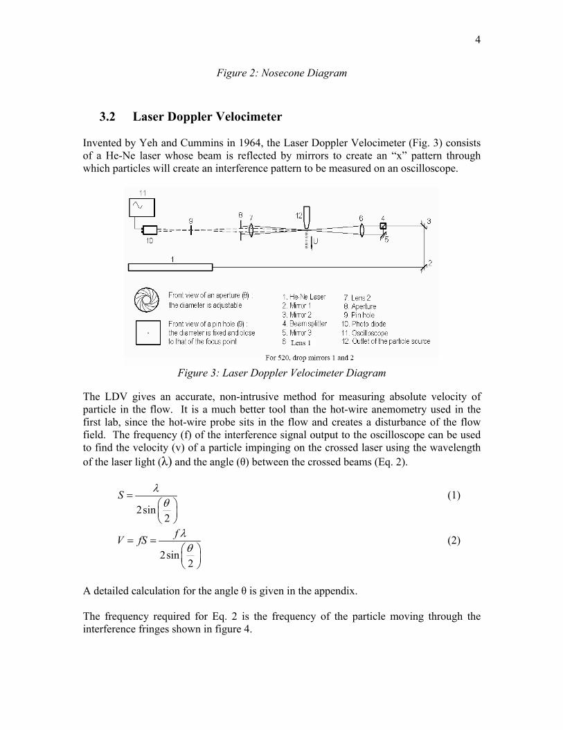
Figure 2: Nosecone Diagram

3.2 Laser Doppler Velocimeter Invented by Yeh and Cummins in 1964, the Laser Doppler Velocimeter (Fig. 3) consists of a He-Ne laser whose beam is reflected by mirrors to create an “x” pattern through which particles will create an interference pattern to be measured on an oscilloscope.

Figure 3: Laser Doppler Velocimeter Diagram

The LDV gives an accurate, non-intrusive method for measuring absolute velocity of particle in the flow. It is a much better tool than the hot-wire anemometry used in the first lab, since the hot-wire probe sits in the flow and creates a disturbance of the flow field. The frequency (f) of the interference signal output to the oscilloscope can be used to find the velocity (v) of a particle impinging on the crossed laser using the wavelength of the laser light (λ) and the angle (θ) between the crossed beams (Eq. 2).

2sin2

S λθ

=

(1)

2sin2

fV fS λθ

= =

(2)

A detailed calculation for the angle θ is given in the appendix. The frequency required for Eq. 2 is the frequency of the particle moving through the interference fringes shown in figure 4.

5

Figure 4: Interference pattern in the LDV With this in mind the LDV will only calculate the component of the velocity of the particle that is moving perpendicularly to the interference fringes

4. Procedure

o Flow Meter Correlation: With an empty test section, the tunnel was run for various readings of the tunnel flow meter ranging from .05 m/s to .28 m/s. For each reading of the flow meter, the velocity was measured using the LDV for comparison.

o Flow Visualization: Dye was injected through the cone at a 30° angle of attack. For various tunnel speeds, the flow was observed and pictures were taken.

o Velocity Distribution of Particles: Since the LDV measures the velocity of only one particle, a statistical analysis of the distribution of velocities in the flow was taken. For an empty tunnel at .089 m/s, the velocity was taken for 10 particles along the centerline of the test section using the LDV.

o Flow Vector Field Around Cone: Velocity measurements were taken in a grid around the tip of the cone for an angle of attack of 35° and freestream velocity of .089 m/s using the LDV.

5. Analysis of Results The Results fall in to 4 major sections where each section describes a major focus of the investigation. Using a digital camera the flow around the cone could be analyzed relatively quickly and easily for a range of velocities. This provided a general understanding of the flow around the cone, and lead to areas of further analysis using the LDV. For these three sections, namely the tunnel calibration, the statistical analysis, and the flow field analysis, there was a great deal of data reduction before meaningful results could be found. It was decided that the raw data from the Laser Doppler Velocimeter should be recorded in terms of a visual output using the scope capture software as well as saving the waveform amplitude and time history data. In this way two possible methods by which the velocity could be found would be available.

6

5.1 Data Reduction The first method by which the data was reduced was to take the visual output from the scope which included both the original wave form along with a filtered waveform. A sample output of the oscilloscope set up for this measurement can be seen in figure 5. The highest plot shows a plot of the unfiltered waveform, and the lower plot shows a plot of a low frequency filter. For this plot the equipment is set up to filter out the low frequency wave in order to show only the higher frequency waveform that is caused by a particle passing through the interference pattern of the lasers.

Figure 5: Oscilloscope output for 3.01 in/s, during calibration run

It is possible to find the velocity from the lower wave pattern by calculating the frequency of the filtered wave from. This was done by counting the number of peaks over a range of time:

# of wavestime interval

f = (3)

An example of this calculation has been included in the appendix for reference. While this provided a reasonable value for the velocity of the run it is a process that can become very time consuming for a large number of data points. It would also be fair to assume that this method can only be applied when a good signal is captured. The filtered waveform in figure 5 shows an example of a very good wave form from one of the calibration runs. The second option was to calculate a Fast Fourier Transform of the data, using a MATLAB script, in order to show the frequency with the highest amplitude directly. The output from a single run from one experiment has been shown in figure 6 (parts a-c).

7

0 0.2 0.4 0.6 0.8 1 1.2 1.4 1.6 1.8 2

x 10-3

-0.035

-0.03

-0.025

-0.02

-0.015

-0.01

-0.005

0

Unfiltered Signal directly from Oscilloscope output - Data set: Calibration, 3.01 inches/second

Time (seconds)

Am

plitu

de

Unfiltered SignalLow fequency polynmial fit

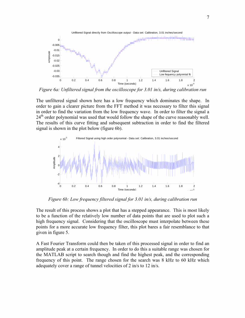
Figure 6a: Unfiltered signal from the oscilloscope for 3.01 in/s, during calibration run

The unfiltered signal shown here has a low frequency which dominates the shape. In order to gain a clearer picture from the FFT method it was necessary to filter this signal in order to find the variation from the low frequency wave. In order to filter the signal a 24th order polynomial was used that would follow the shape of the curve reasonably well. The results of this curve fitting and subsequent subtraction in order to find the filtered signal is shown in the plot below (figure 6b).

0 0.2 0.4 0.6 0.8 1 1.2 1.4 1.6 1.8 2

x 10-3

-4

-2

0

2

4

x 10-3 Filtered Signal using high order polynomial - Data set: Calibration, 3.01 inches/second

Time (seconds)

Am

plitu

de

Figure 6b: Low frequency filtered signal for 3.01 in/s, during calibration run The result of this process shows a plot that has a stepped appearance. This is most likely to be a function of the relatively low number of data points that are used to plot such a high frequency signal. Considering that the oscilloscope must interpolate between these points for a more accurate low frequency filter, this plot bares a fair resemblance to that given in figure 5. A Fast Fourier Transform could then be taken of this processed signal in order to find an amplitude peak at a certain frequency. In order to do this a suitable range was chosen for the MATLAB script to search though and find the highest peak, and the corresponding frequency of this point. The range chosen for the search was 8 kHz to 60 kHz which adequately cover a range of tunnel velocities of 2 in/s to 12 in/s.

8

x 10( )

1 1.5 2 2.5 3 3.5 4 4.5 5 5.5 6

x 104

0

0.2

0.4

0.6

0.8

1

1.2

Shifted FFT of filtered signal - Data set: Calibration, 3.01 inches/second

Frequency (Hz)

Am

plitu

de

Frequency =13008.1177 Hz

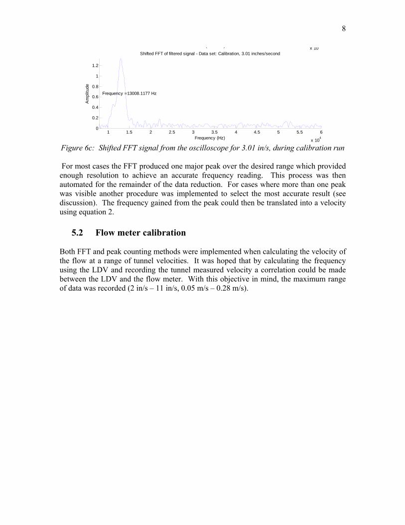
Figure 6c: Shifted FFT signal from the oscilloscope for 3.01 in/s, during calibration run

For most cases the FFT produced one major peak over the desired range which provided enough resolution to achieve an accurate frequency reading. This process was then automated for the remainder of the data reduction. For cases where more than one peak was visible another procedure was implemented to select the most accurate result (see discussion). The frequency gained from the peak could then be translated into a velocity using equation 2.

5.2 Flow meter calibration Both FFT and peak counting methods were implemented when calculating the velocity of the flow at a range of tunnel velocities. It was hoped that by calculating the frequency using the LDV and recording the tunnel measured velocity a correlation could be made between the LDV and the flow meter. With this objective in mind, the maximum range of data was recorded (2 in/s – 11 in/s, 0.05 m/s – 0.28 m/s).

9

Velocity Correlation using peak counting method y = 1.2486x - 0.0118R2 = 0.9574

0

0.05

0.1

0.15

0.2

0.25

0.3

0.35

0.4

0 0.05 0.1 0.15 0.2 0.25 0.3 0.35 0.4

Flow Meter Velocity (m/s)

Mea

sure

d Ve

loci

ty (m

/s)

Figure 7: Velocity Correlation Between Flow Meter Reading and LDV Signal Using

Peak Counting Method of Calculation

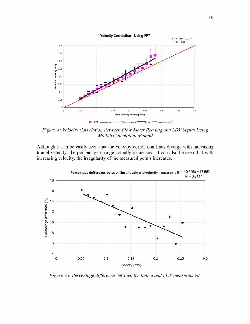
The result for the peak counting method is shown in figure 7. The plot shows a close correlation with the tunnel reading although significantly higher, suggesting that the tunnel reading underestimates the actual velocity in the tunnel by 10 – 15%. The plot only shows a range of velocities up to 0.18m/s (7in/s) as the peak counting method could not be implemented with the same accuracy above this point to achieve a meaningful result. For higher velocities, the counting by eye method became much more difficult for measuring peaks as they get much closer together on the scope picture. Even with adjustment of the aspect ratio it was found that the low resolution prohibited an accurate result to be taken. Errors in velocity data are computed in the appendix. Using the FFT method a very similar plot was achieved (figure 8). It was possible to gain a greater range in the calibration line. For lower velocities however the plots give almost identical results suggesting that the accuracy of the data may be more influenced by the generation of the signal, rather than the quality of the interpretation of the result.

10

Velocity Correlation - Using FFTy = 1.1431x - 0.0014

R2 = 0.9844

0

0.05

0.1

0.15

0.2

0.25

0.3

0.35

0.4

0 0.05 0.1 0.15 0.2 0.25 0.3 0.35 0.4

Tunnel Velocity Reading (m/s)

Mea

sure

d Ve

loci

ty (m

/s)

FFT measurement Tunnel reading Linear (FFT measurement)

Figure 8: Velocity Correlation Between Flow Meter Reading and LDV Signal Using

Matlab Calculation Method

Although it can be easily seen that the velocity correlation lines diverge with increasing tunnel velocity, the percentage change actually decreases. It can also be seen that with increasing velocity, the irregularity of the measured points increases.

Percentage defference between linear scale and velocity measurementy = -40.626x + 17.562R2 = 0.7117

4

6

8

10

12

14

16

18

0 0.05 0.1 0.15 0.2 0.25 0.3

Velocity (m/s)

Perc

enta

ge d

iffer

ence

(%)

Figure 9a: Percentage difference between the tunnel and LDV measurement,

11

Error in Velocity Measurement y = 0.1339x + 0.0011R2 = 0.7522

0.00

0.01

0.02

0.03

0.04

0.05

0.06

0 0.05 0.1 0.15 0.2 0.25 0.3Velocity (m/s)

Erro

r

Figure 9b: Error in velocity measurement for the FFT method

This suggests that with increase in velocity one error form is being traded for another. This theory can be depicted figure 9a and figure 9b. The equations for correlating the flow meter velocity reading and the measured velocity are given in Table 1 along with the R2 value, which is a measurement of the accuracy of the linear fit.

Table 1: Summary of Velocity Correlation Between Flow Meter Reading (X) and Measured Velocity (Y)

Eye Calculation Matlab Calculation Equation 1.2486 0.0118Y X= − 1.1431 0.0014Y X= × −

R2 .9574 .9844 The equation relations show a difference of around 10%. The least squares value also suggests that the matlab calculation is more accurate than the peak counting method. This least squares value has also been taken over a greater range of velocities showing that the method provides both greater accuracy and a larger measurement window.

5.3 Statistical analysis of the velocity data A statistical analysis was performed with no model in the tunnel in order to examine the distribution of velocities of particles within the water tunnel. This is a vital part of the

12

experiment as a narrow distribution of velocities will give validity to the velocity results gained, whereas a wide distribution can negate the purpose of the experiment. A series of 10 results have been plotted according to a set of 5 velocity ranges. This analysis can be seen in figure 10.

Statistical analysis of velocity data

012345

0.099

1 - 0.

0999

0.099

9 - 0.

1007

0.100

7 - 0.

1015

0.101

5 - 0.

1023

0.102

3 - 0.

1031

Velocity (m/s)

Num

ber o

f par

ticle

s Measured VelocitiesNormal Distribution

Figure 10: Statistical analysis, 10 data points over a velocity range of 0.0991 – 0.1031

m/s (3.9 – 4.0 in/s) The statistical plot shows a resemblance to a normal distribution. Given more time and a great deal more data points, it should be possible to show a distribution that accurately matches the normal curve. The figure also gives a very small range in velocity fluctuations suggesting that the LDV is very accurate, and that by taking an average of a number of results should narrow this error source even further.

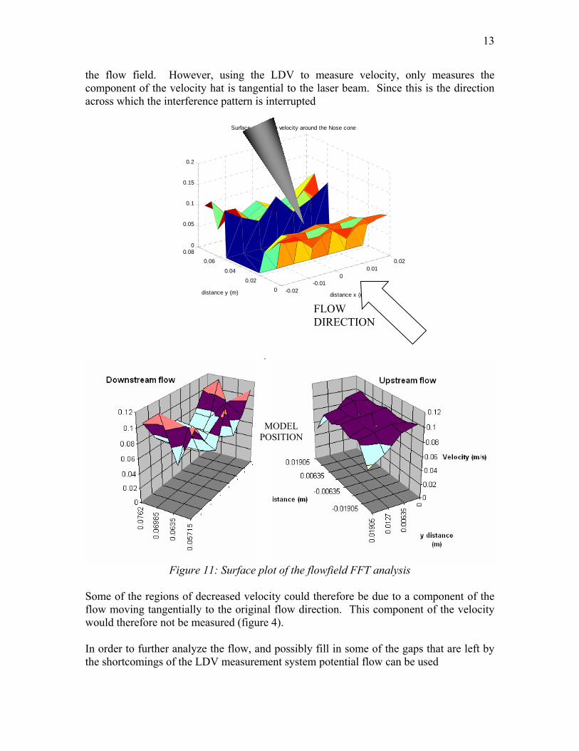
5.4 Flowfield analysis around the tip of the cone The major focus for the experiment was to attempt to map a velocity profile around the tip of the cone. By taking regularly spaced readings of velocity in a grid pattern around the cone it was possibly to generate a profile describing how the velocity changes around the cone. By careful adjustments of the cone in the x direction and traversing the LDV in the y direction a grid of points was generated around the tip of the cone. Unfortunately since the LDV requires the laser to travel the full width of the tunnel it was impossible to take results at the sides of the cone with the current configuration of apparatus. The result is therefore a fore and aft comparison of the flow around the cone. An initial comparison of the upstream and downstream effects of the cone has been made in figure 11. The figure shows contours of velocity in the downstream direction. The result is a decrease in velocity before the cone, a region of low velocity in the wake of the cone, and a much less uniform shape behind the cone. The results seem at first unintuitive, as the flow is running at its fastest velocity in the centre and at the edges of

13

the flow field. However, using the LDV to measure velocity, only measures the component of the velocity hat is tangential to the laser beam. Since this is the direction across which the interference pattern is interrupted

-0.02-0.01

00.01

0.02

0

0.02

0.04

0.06

0.080

0.05

0.1

0.15

0.2

distance x (m)

Surface plot of the velocity around the Nose cone

distance y (m)

Figure 11: Surface plot of the flowfield FFT analysis

Some of the regions of decreased velocity could therefore be due to a component of the flow moving tangentially to the original flow direction. This component of the velocity would therefore not be measured (figure 4). In order to further analyze the flow, and possibly fill in some of the gaps that are left by the shortcomings of the LDV measurement system potential flow can be used

MODEL POSITION

FLOW DIRECTION

14

5.5 Analysis of potential flow around a cylinder

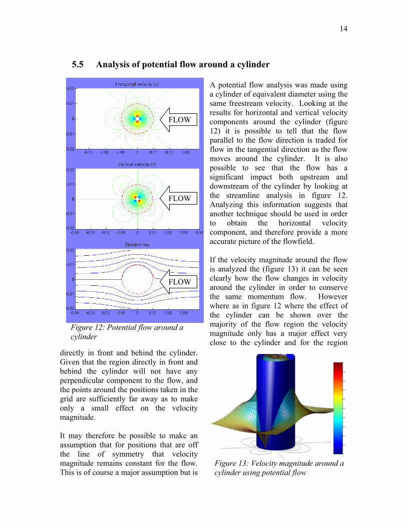
A potential flow analysis was made using a cylinder of equivalent diameter using the same freestream velocity. Looking at the results for horizontal and vertical velocity components around the cylinder (figure 12) it is possible to tell that the flow parallel to the flow direction is traded for flow in the tangential direction as the flow moves around the cylinder. It is also possible to see that the flow has a significant impact both upstream and downstream of the cylinder by looking at the streamline analysis in figure 12. Analyzing this information suggests that another technique should be used in order to obtain the horizontal velocity component, and therefore provide a more accurate picture of the flowfield. If the velocity magnitude around the flow is analyzed the (figure 13) it can be seen clearly how the flow changes in velocity around the cylinder in order to conserve the same momentum flow. However where as in figure 12 where the effect of the cylinder can be shown over the majority of the flow region the velocity magnitude only has a major effect very close to the cylinder and for the region

directly in front and behind the cylinder. Given that the region directly in front and behind the cylinder will not have any perpendicular component to the flow, and the points around the positions taken in the grid are sufficiently far away as to make only a small effect on the velocity magnitude. It may therefore be possible to make an assumption that for positions that are off the line of symmetry that velocity magnitude remains constant for the flow. This is of course a major assumption but is

Figure 13: Velocity magnitude around a cylinder using potential flow

FLOW

FLOW

FLOW

Figure 12: Potential flow around a cylinder

15

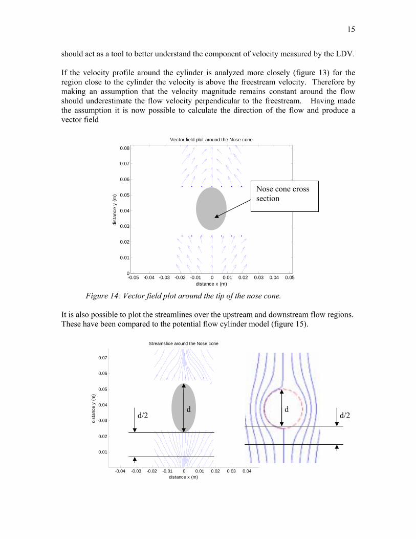
should act as a tool to better understand the component of velocity measured by the LDV. If the velocity profile around the cylinder is analyzed more closely (figure 13) for the region close to the cylinder the velocity is above the freestream velocity. Therefore by making an assumption that the velocity magnitude remains constant around the flow should underestimate the flow velocity perpendicular to the freestream. Having made the assumption it is now possible to calculate the direction of the flow and produce a vector field

-0.05 -0.04 -0.03 -0.02 -0.01 0 0.01 0.02 0.03 0.04 0.050

0.01

0.02

0.03

0.04

0.05

0.06

0.07

0.08

Vector field plot around the Nose cone

distance x (m)

dist

ance

y (

m)

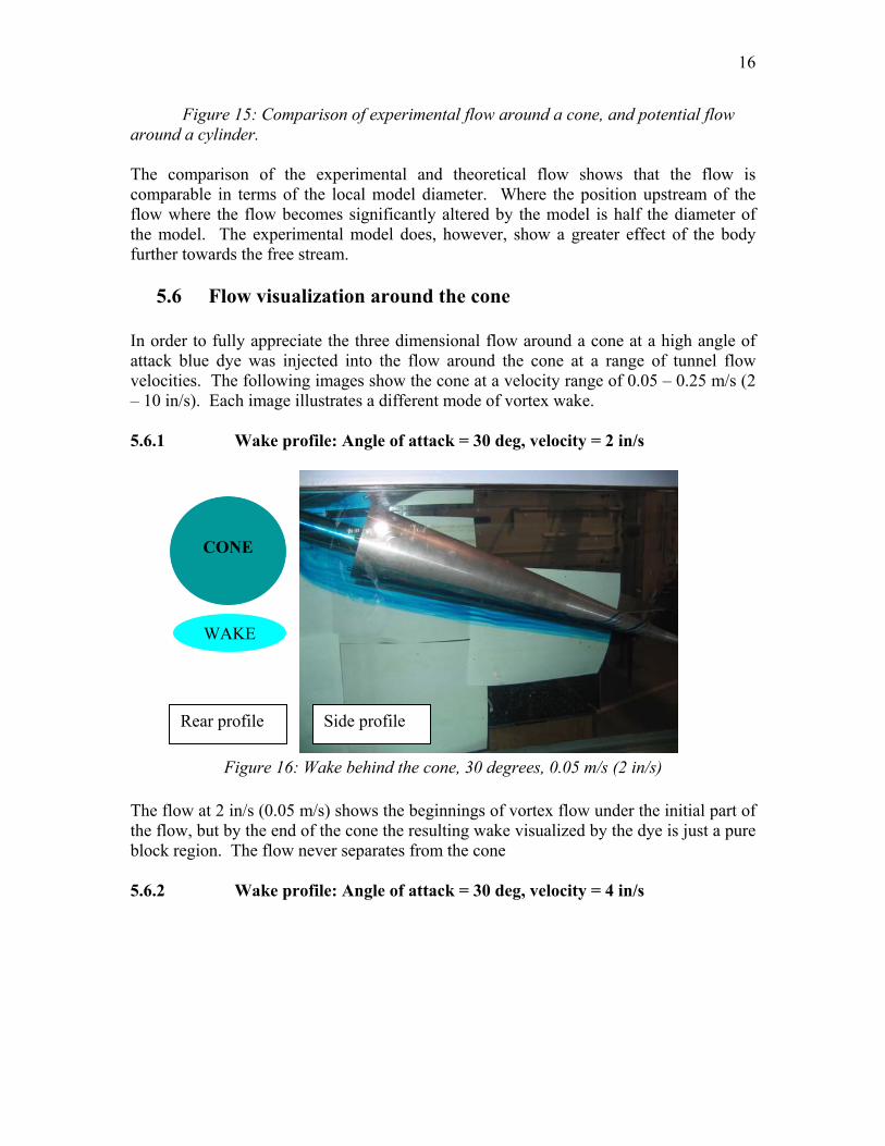
Figure 14: Vector field plot around the tip of the nose cone. It is also possible to plot the streamlines over the upstream and downstream flow regions. These have been compared to the potential flow cylinder model (figure 15).

-0.04 -0.03 -0.02 -0.01 0 0.01 0.02 0.03 0.04

0.01

0.02

0.03

0.04

0.05

0.06

0.07

Streamslice around the Nose cone

distance x (m)

dist

ance

y (

m)

Nose cone cross section

d d d/2 d/2

16

Figure 15: Comparison of experimental flow around a cone, and potential flow around a cylinder. The comparison of the experimental and theoretical flow shows that the flow is comparable in terms of the local model diameter. Where the position upstream of the flow where the flow becomes significantly altered by the model is half the diameter of the model. The experimental model does, however, show a greater effect of the body further towards the free stream.

5.6 Flow visualization around the cone In order to fully appreciate the three dimensional flow around a cone at a high angle of attack blue dye was injected into the flow around the cone at a range of tunnel flow velocities. The following images show the cone at a velocity range of 0.05 – 0.25 m/s (2 – 10 in/s). Each image illustrates a different mode of vortex wake. 5.6.1 Wake profile: Angle of attack = 30 deg, velocity = 2 in/s

Figure 16: Wake behind the cone, 30 degrees, 0.05 m/s (2 in/s)

The flow at 2 in/s (0.05 m/s) shows the beginnings of vortex flow under the initial part of the flow, but by the end of the cone the resulting wake visualized by the dye is just a pure block region. The flow never separates from the cone 5.6.2 Wake profile: Angle of attack = 30 deg, velocity = 4 in/s

CONE

WAKE

Rear profile Side profile

17

Figure 17: Wake behind the cone, 30 degrees, 4 in/s

At 4 in/s (0.1 m/s) there are two clear vortices indicated by the dye flow. These two vortices are complemented by two regions of purely laminar flow containing dye. Separation does not occur. 5.6.3 Wake profile: Angle of attack = 30 deg, velocity = 6 in/s

Figure 18: Wake behind the cone, 30 degrees, 6 in/s (0.15 m/s) The profile behind the cone at 6 in/s (0.15 m/s) is very similar to the profile at 4 in/s, however there are 4 vortices in the wake. The two laminar flow regions discussed in the 4 in/s case transition to vortex flow to yield 4 vortices in the wake. These vortices remain attached to the cone for its entire length.

V V

CONE


V V

CONE

V V


18

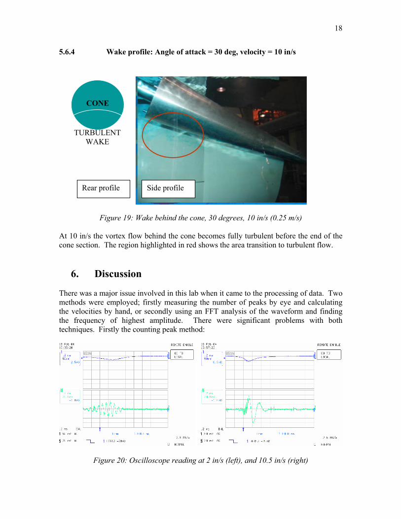
5.6.4 Wake profile: Angle of attack = 30 deg, velocity = 10 in/s

Figure 19: Wake behind the cone, 30 degrees, 10 in/s (0.25 m/s) At 10 in/s the vortex flow behind the cone becomes fully turbulent before the end of the cone section. The region highlighted in red shows the area transition to turbulent flow.

6. Discussion There was a major issue involved in this lab when it came to the processing of data. Two methods were employed; firstly measuring the number of peaks by eye and calculating the velocities by hand, or secondly using an FFT analysis of the waveform and finding the frequency of highest amplitude. There were significant problems with both techniques. Firstly the counting peak method:

Figure 20: Oscilloscope reading at 2 in/s (left), and 10.5 in/s (right)

CONE

TURBULENT

WAKE


19

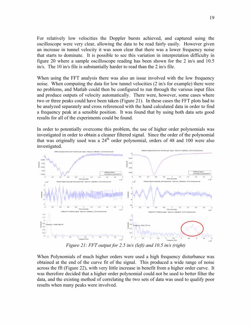
For relatively low velocities the Doppler bursts achieved, and captured using the oscilloscope were very clear, allowing the data to be read fairly easily. However given an increase in tunnel velocity it was soon clear that there was a lower frequency noise that starts to dominate. It is possible to see this variation in interpretation difficulty in figure 20 where a sample oscilloscope reading has been shown for the 2 in/s and 10.5 in/s. The 10 in/s file is substantially harder to read than the 2 in/s file. When using the FFT analysis there was also an issue involved with the low frequency noise. When computing the data for low tunnel velocities (2 in/s for example) there were no problems, and Matlab could then be configured to run through the various input files and produce outputs of velocity automatically. There were, however, some cases where two or three peaks could have been taken (Figure 21). In these cases the FFT plots had to be analyzed separately and cross referenced with the hand calculated data in order to find a frequency peak at a sensible position. It was found that by using both data sets good results for all of the experiments could be found. In order to potentially overcome this problem, the use of higher order polynomials was investigated in order to obtain a cleaner filtered signal. Since the order of the polynomial that was originally used was a 24th order polynomial, orders of 48 and 100 were also investigated.

0 0.2 0.4 0.6 0.8 1 1.2 1.4 1.6 1.8 2

x 10-3

-0.025

-0.02

-0.015

-0.01

-0.005

0


Time (seconds)

Am

plitu

de


0 0.2 0.4 0.6 0.8 1 1.2 1.4 1.6 1.8 2

x 10-3

-4

-2

0

2

4


Time (seconds)

Am

plitu

de

1 1.5 2 2.5 3 3.5 4 4.5 5 5.5 6

x 104

0

0.2

0.4

0.6

0.8

1

1.2

1.4


Frequency (Hz)

Am

plitu

de


0 0.2 0.4 0.6 0.8 1 1.2 1.4 1.6 1.8 2

x 10-3

-0.08

-0.06

-0.04

-0.02

0


Time (seconds)

Am

plitu

de


0 0.2 0.4 0.6 0.8 1 1.2 1.4 1.6 1.8 2

x 10-3

-10

-5

0

5


Time (seconds)

Am

plitu

de

1 1.5 2 2.5 3 3.5 4 4.5 5 5.5 6

x 104

0

0.2

0.4

0.6

0.8

1


Frequency (Hz)

Am

plitu

de


Figure 21: FFT output for 2.5 in/s (left) and 10.5 in/s (right)

When Polynomials of much higher orders were used a high frequency disturbance was obtained at the end of the curve fit of the signal. This produced a wide range of noise across the fft (Figure 22), with very little increase in benefit from a higher order curve. It was therefore decided that a higher order polynomial could not be used to better filter the data, and the existing method of correlating the two sets of data was used to qualify poor results when many peaks were involved.

20

0 0.2 0.4 0.6 0.8 1 1.2 1.4 1.6 1.8 2

x 10-3

-0.08

-0.06

-0.04

-0.02

0


Time (seconds)

Am

plitu

de


0 0.2 0.4 0.6 0.8 1 1.2 1.4 1.6 1.8 2

x 10-3

-5

0

5

10


Time (seconds)

Am

plitu

de

1 1.5 2 2.5 3 3.5 4 4.5 5 5.5 6

x 104

0

0.1

0.2

0.3

0.4

0.5

0.6

0.7Shifted FFT of filtered signal - Data set: Calibration, 10.51 inches/second

Frequency (Hz)

Am

plitu

de


0 0.2 0.4 0.6 0.8 1 1.2 1.4 1.6 1.8 2

x 10-3

-0.08

-0.06

-0.04

-0.02

0


Time (seconds)

Am

plitu

de


0 0.2 0.4 0.6 0.8 1 1.2 1.4 1.6 1.8 2

x 10-3

-0.01

-0.005

0

0.005

0.01

0.015Filtered Signal using high order polynomial - Data set: Calibration, 10.51 inches/second

Time (seconds)

Am

plitu

de

1 1.5 2 2.5 3 3.5 4 4.5 5 5.5 6

x 104

0

0.1

0.2

0.3

0.4

0.5

0.6


Frequency (Hz)

Am

plitu

de


Figure 22: FFT output for 10.5 in/s using a 48 order polynomial (left) and a 100 order

polynomial (right)

7. Conclusion

After completing this lab, much experience was gained using the water tunnel, LDV, and flow dye equipment. Data for the correlation between the tunnel flow meter and actual velocity measured with the LDV was obtained. Data using our FFT method proved more reliable than counting peaks by eye, although precision increases at higher velocity for both methods. We should have adjusted the time/division adjustment on the scope to aid better results at higher velocities, but there is still some inherent error in the signal due to an unsymmetrical Doppler signal (Fig. 20). Adjustment of the LDV would correct this problem. A more accurate measurement of the angle between the crossed laser beams could be given either through a more precise measurement or increasing the angle. This would eliminate a good portion of our error due to computing velocities. The statistical analysis of the velocity data proves that the computation error in our velocity data for the flow meter correlation is much larger than the distribution of velocities for various particles at a set tunnel speed. Thus, measuring only one particle for each tunnel speed was a reasonable thing to do. To better aid our results in this section, data for a larger number of particles would fill in our distribution better. Considering our results for the velocity grid around the tip of the cone, the results seem to match up with potential flow and CFD solutions. Taking these readings at a relatively low tunnel speed (3.5 in/s or .089 m/s) enabled us to reduce turbulent fluctuations in downstream velocity readings. One limiting factor on our results is that when resolving

21

the LVD velocity measurements into two components we are ignore the fact that the flow is three dimensional. Another contributor to error is the fact that when measuring velocities across the tunnel, the model is moved (not the LVD system) introducing errors from side wall effects (although we stayed away from the side as much as possible). For better results, One error in all measurements that has yet to be mentioned is the contribution of surface on the freestream velocity value.

8. References [1] Fluid Mechanics measurements, Richard J. Goldstein [2] Mechanics of Fluids, Bernard Massey [3] LDV introduction, http://roger.ecn.purdue.edu/~aae520/LDv-lecture-rev2.pdf

9. APPENDIX SAMPLE CALCULATIONS:

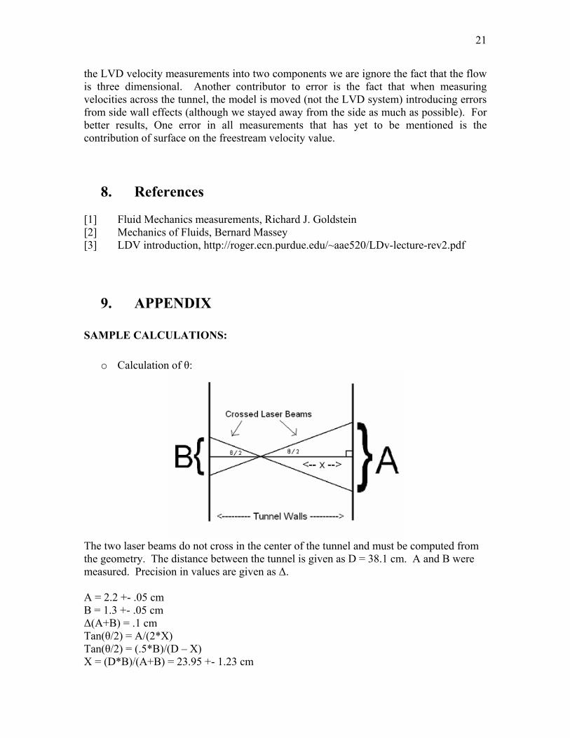
o Calculation of θ:

The two laser beams do not cross in the center of the tunnel and must be computed from the geometry. The distance between the tunnel is given as D = 38.1 cm. A and B were measured. Precision in values are given as ∆. A = 2.2 +- .05 cm B = 1.3 +- .05 cm ∆(A+B) = .1 cm Tan(θ/2) = A/(2*X) Tan(θ/2) = (.5*B)/(D – X) X = (D*B)/(A+B) = 23.95 +- 1.23 cm

22

∆X = X*[(∆B/B) + ∆(A+B)/(A+B)] = 1.23 cm Knowing X, θ can be calculated from above. θ = 2*tan-1[A/(2*X)] = 5.26 +- .51° A rough estimate of ∆θ is given below. ∆θ = .5* | tan-1[(A+∆A)/(2*(X-∆X))] - tan-1[(A-∆A)/(2*(X+∆X))] | = .51°

o Calculation of velocity by eye: f = (# of waves)/(time interval) Sample: f = 9 waves /(5*0.0002 sec) = 9000 Hz ∆f = (9 + .25)/(5*0.0002 sec) – f = 250 Hz (the accuracy of my count was +- .25 waves, I counted in increments of .25 waves) λ = 633E-9 m s = λ/[2*sin(θ/2)] = (6.90 +- .52) E-6 m ∆{sin(θ/2)} = .5* | sin{(θ+∆θ) /2} - sin{(θ-∆θ) /2} | = 3.5E-6 ∆s = s*[(∆λ/λ) + (∆{sin(θ/2)}/ sin(θ/2))] v = f*s = .062 +- .006 m/s ∆v = v*[(∆f/f) + (∆s/s)] = .006 m/s

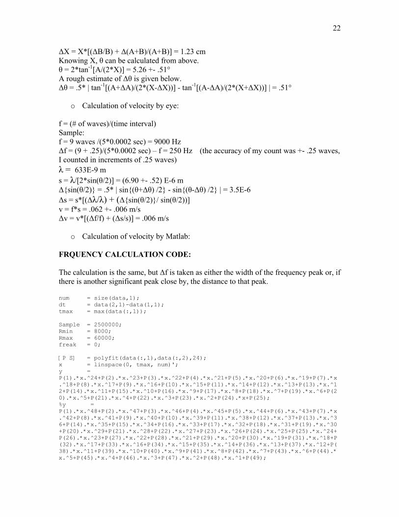
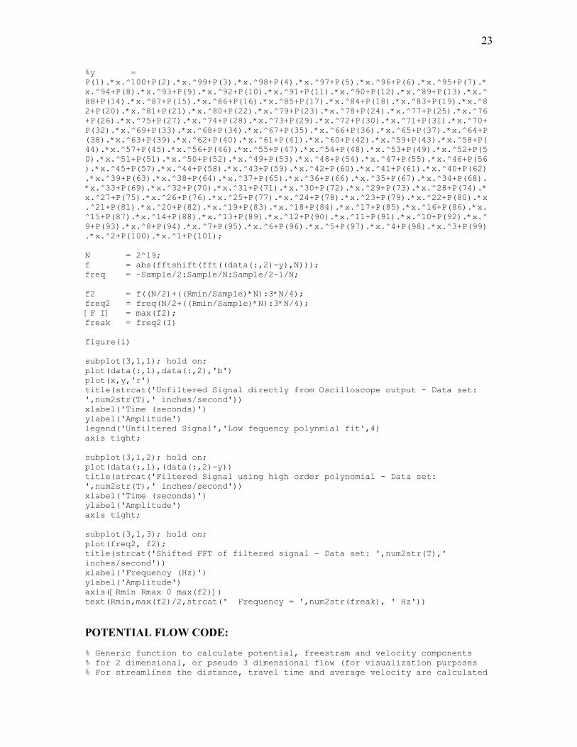
o Calculation of velocity by Matlab: FRQUENCY CALCULATION CODE: The calculation is the same, but ∆f is taken as either the width of the frequency peak or, if there is another significant peak close by, the distance to that peak. num = size(data,1); dt = data(2,1)-data(1,1); tmax = max(data(:,1)); Sample = 2500000; Rmin = 8000; Rmax = 60000; freak = 0; [P S] = polyfit(data(:,1),data(:,2),24); x = linspace(0, tmax, num)'; y = P(1).*x.^24+P(2).*x.^23+P(3).*x.^22+P(4).*x.^21+P(5).*x.^20+P(6).*x.^19+P(7).*x.^18+P(8).*x.^17+P(9).*x.^16+P(10).*x.^15+P(11).*x.^14+P(12).*x.^13+P(13).*x.^12+P(14).*x.^11+P(15).*x.^10+P(16).*x.^9+P(17).*x.^8+P(18).*x.^7+P(19).*x.^6+P(20).*x.^5+P(21).*x.^4+P(22).*x.^3+P(23).*x.^2+P(24).*x+P(25); %y = P(1).*x.^48+P(2).*x.^47+P(3).*x.^46+P(4).*x.^45+P(5).*x.^44+P(6).*x.^43+P(7).*x.^42+P(8).*x.^41+P(9).*x.^40+P(10).*x.^39+P(11).*x.^38+P(12).*x.^37+P(13).*x.^36+P(14).*x.^35+P(15).*x.^34+P(16).*x.^33+P(17).*x.^32+P(18).*x.^31+P(19).*x.^30+P(20).*x.^29+P(21).*x.^28+P(22).*x.^27+P(23).*x.^26+P(24).*x.^25+P(25).*x.^24+P(26).*x.^23+P(27).*x.^22+P(28).*x.^21+P(29).*x.^20+P(30).*x.^19+P(31).*x.^18+P(32).*x.^17+P(33).*x.^16+P(34).*x.^15+P(35).*x.^14+P(36).*x.^13+P(37).*x.^12+P(38).*x.^11+P(39).*x.^10+P(40).*x.^9+P(41).*x.^8+P(42).*x.^7+P(43).*x.^6+P(44).*x.^5+P(45).*x.^4+P(46).*x.^3+P(47).*x.^2+P(48).*x.^1+P(49);

23

%y = P(1).*x.^100+P(2).*x.^99+P(3).*x.^98+P(4).*x.^97+P(5).*x.^96+P(6).*x.^95+P(7).*x.^94+P(8).*x.^93+P(9).*x.^92+P(10).*x.^91+P(11).*x.^90+P(12).*x.^89+P(13).*x.^88+P(14).*x.^87+P(15).*x.^86+P(16).*x.^85+P(17).*x.^84+P(18).*x.^83+P(19).*x.^82+P(20).*x.^81+P(21).*x.^80+P(22).*x.^79+P(23).*x.^78+P(24).*x.^77+P(25).*x.^76+P(26).*x.^75+P(27).*x.^74+P(28).*x.^73+P(29).*x.^72+P(30).*x.^71+P(31).*x.^70+P(32).*x.^69+P(33).*x.^68+P(34).*x.^67+P(35).*x.^66+P(36).*x.^65+P(37).*x.^64+P(38).*x.^63+P(39).*x.^62+P(40).*x.^61+P(41).*x.^60+P(42).*x.^59+P(43).*x.^58+P(44).*x.^57+P(45).*x.^56+P(46).*x.^55+P(47).*x.^54+P(48).*x.^53+P(49).*x.^52+P(50).*x.^51+P(51).*x.^50+P(52).*x.^49+P(53).*x.^48+P(54).*x.^47+P(55).*x.^46+P(56).*x.^45+P(57).*x.^44+P(58).*x.^43+P(59).*x.^42+P(60).*x.^41+P(61).*x.^40+P(62).*x.^39+P(63).*x.^38+P(64).*x.^37+P(65).*x.^36+P(66).*x.^35+P(67).*x.^34+P(68).*x.^33+P(69).*x.^32+P(70).*x.^31+P(71).*x.^30+P(72).*x.^29+P(73).*x.^28+P(74).*x.^27+P(75).*x.^26+P(76).*x.^25+P(77).*x.^24+P(78).*x.^23+P(79).*x.^22+P(80).*x.^21+P(81).*x.^20+P(82).*x.^19+P(83).*x.^18+P(84).*x.^17+P(85).*x.^16+P(86).*x.^15+P(87).*x.^14+P(88).*x.^13+P(89).*x.^12+P(90).*x.^11+P(91).*x.^10+P(92).*x.^9+P(93).*x.^8+P(94).*x.^7+P(95).*x.^6+P(96).*x.^5+P(97).*x.^4+P(98).*x.^3+P(99).*x.^2+P(100).*x.^1+P(101); N = 2^19; f = abs(fftshift(fft((data(:,2)-y),N))); freq = -Sample/2:Sample/N:Sample/2-1/N; f2 = f((N/2)+((Rmin/Sample)*N):3*N/4); freq2 = freq(N/2+((Rmin/Sample)*N):3*N/4); [F I] = max(f2); freak = freq2(I) figure(i) subplot(3,1,1); hold on; plot(data(:,1),data(:,2),'b') plot(x,y,'r') title(strcat('Unfiltered Signal directly from Oscilloscope output - Data set: ',num2str(T),' inches/second')) xlabel('Time (seconds)') ylabel('Amplitude') legend('Unfiltered Signal','Low fequency polynmial fit',4) axis tight; subplot(3,1,2); hold on; plot(data(:,1),(data(:,2)-y)) title(strcat('Filtered Signal using high order polynomial - Data set: ',num2str(T),' inches/second')) xlabel('Time (seconds)') ylabel('Amplitude') axis tight; subplot(3,1,3); hold on; plot(freq2, f2); title(strcat('Shifted FFT of filtered signal - Data set: ',num2str(T),' inches/second')) xlabel('Frequency (Hz)') ylabel('Amplitude') axis([Rmin Rmax 0 max(f2)]) text(Rmin,max(f2)/2,strcat(' Frequency = ',num2str(freak), ' Hz'))

POTENTIAL FLOW CODE: % Generic function to calculate potential, freestram and velocity components % for 2 dimensional, or pseudo 3 dimensional flow (for visualization purposes % For streamlines the distance, travel time and average velocity are calculated

24

% Polar coordinates r = sqrt(x.^2 + y.^2); theta = atan2(y,x); % Cylinder coordinates [xc,yc,zc]= cylinder(rc); zc = zc.*(1.2*depth); % Uniform horizontal flow phi_fs = +u_inf.*x; psi_fs = +u_inf.*y; vrad_fs = +u_inf.*cos(theta); vtan_fs = -u_inf.*sin(theta); % Doublet flow phi_d = +(kappa.*cos(theta))./(2*pi.*r); psi_d = -(kappa.*sin(theta))./(2*pi.*r); vrad_d = -(kappa.*cos(theta))./(2*pi.*r.^2); vtan_d = -(kappa.*sin(theta))./(2*pi.*r.^2); % Point vortex flow phi_v = -(gamma/(2*pi)).*theta; psi_v = +(gamma/(2*pi)).*log(r./rc); vrad_v = 0; vtan_v = -(gamma./(2*pi.*r)); % Total flow phi = phi_fs + phi_v + phi_d; psi = psi_fs + psi_v + psi_d; vtan = vtan_fs + vtan_v + vtan_d; vrad = vrad_fs + vrad_v + vrad_d; % Velocity components u = vrad.*cos(theta) - vtan.*sin(theta); v = vrad.*sin(theta) + vtan.*cos(theta); w = v.*0; vmag = sqrt(u.^2 + v.^2 + w.^2); % Results if size(x,2) == 1 % Only calculated for streamlines S = sum(sqrt(diff(x).^2 +diff(y).^2)); ds = cumsum(sqrt(diff(x).^2 +diff(y).^2)); ds = cat(1,0,ds); T = trapz(ds,1./vmag); Vavg = S/T; elseif size(z,3) ~= 1 % Only calculated if the grid is 3D cav = curl(x,y,z,u,v,w); XYZ = stream3(x,y,z,u,v,w,xs,ys,zs); end

Documents

Experiment 3 - Purdue Engineeringaae520/kay-chibana-520-Lab3.pdf3 3. Background 3.1 Water Tunnel The water tunnel (Fig. 1) operates as a continuous flow channel pumping 1,000 gallons